Global Optimization to Real Time Control of HEV Power Flow: Example of a Fuel Cell Hybrid Vehicle

Sylvain Pagerit, Aymeric Rousseau, Phil Sharer

Abstract

Hybrid Electrical Vehicle (HEV) fuel economy highly depends on power allocation between the different power sources — engine and fuel cell — and the energy storage system(s). A generic global optimization algorithm has been developed to minimize fuel consumption by optimizing the powertrain power flows. This algorithm was applied on a Fuel Cell Hybrid Vehicle, and results were generated for several driving cycles. By using these results, a real-time control strategy was developed and implemented in PSAT (Powertrain System Analysis Toolkit). Methodology, as well as control strategy differences, will be discussed.

Keywords: HEV, controller, optimization, simulation, fuel cell.

1 Introduction Hybrid Electrical Vehicles (HEVs) are undergoing extensive research and development because of their potential for high efficiency and low emissions. Their controls, like those for any other vehicle, have to maximize fuel economy, which in this case, is highly dependent on the power allocation between the fuel converters (engine and fuel cell) and the energy storage system(s). Different instantaneous and global optimization algorithms have been defined in the past to understand the behavior of such control for HEVs [1–5]. For instantaneous optimization, the results can lead to local minima, with control behavior different from the global optimum. Moreover, the global optimization considered is specific to a given vehicle configuration and cannot be easily adapted. In this paper, a generic global optimization algorithm on the powertrain flows has been developed on the basis of the Bellman optimality principle. The most efficient power flow control for a given cycle can then be computed for different powertrain configurations. The optimization algorithm was then applied to a fuel cell hybrid vehicle with a fixed transmission ratio. This configuration allows for a reduced state and command space, thereby reducing the computation time needed to validate the algorithm and find the optimal command. For the same purpose, the vehicle is simulated by using static component models and backward simulation. The optimization results are used to isolate control patterns, both dependent and independent of the cycle characteristics in order to develop real-time control strategies in Simulink/Stateflow. These controllers are then implemented in PSAT to validate their performances. PSAT is a “forward-looking” model that simulates fuel economy and performance in a realistic manner by taking into account transient behavior and control system characteristics. It can simulate an unrivaled number of predefined configurations (conventional, electric, fuel cell, series hybrid, parallel hybrid, and power split hybrid). Because of its forward architecture, PSAT component interactions are “real world.”

Pcmd = Pout + L(e,f) Pout

U ~ cst I = (Pout / ρ(U,I) + L(U,I)) / U ∆SOC = F(∆I)

Pout

Pi,in=ωi.Ti ωi,in=ωout / ρi(ωout,Tout) Ti,in = Tout . ρi(ωout,Tout) + Li(ωout,Tout) / ωi,in

Pout

PSAT has been validated within 5% accuracy by using testing results from several vehicles and is currently the preferred vehicle simulation tool for DOE’s FreedomCAR& Fuels Partnership activities.

2 HEV Power Flows Modeling and Control

2.1 Static Power Flow Modeling

When using optimization algorithms, the number of computations is a critical factor that must be minimized to find a solution within a reasonable amount of time. For this reason, simplified static component models can be used for backward simulation of the HEV. Hence, focusing only on the power flow, most components can be modeled as shown in Figure 1:

Figure 1: 1st Order Static Model for Backward Simulation Where P = e.f is the power, e is the effort (e.g., torque), f is the flow (e.g., rotational speed), ρ is the reduction ratio, and L is the Power Loss. The other components consist of three different groups:

Power Source (Fuel Cell or Engine):

Energy Storage (again, to reduce computation time and as a first approach, the voltage is considered about constant, but the ratio and losses are different, pending the energy storage system [ESS] state — charging or discharging):

Transmission ( Ngi ,0 0: neutral, Ng: number of gears: Therefore, by using these static models, most HEV power flows can be represented as a combination of the following layout (Figure 2):

Figure 2: HEV Power Flows Where:

MPS: Mechanical Power Source, which consists of either or Eng FC PP E/M C

EPS

PP

E/M C

MPS PP

PP WhA Veh

WhA 2

Series

Conventional, Parallel, Split

Series, Parallel, Split

Propelling

Regen

Electrical Node

Mechanical Node (1)

(3)

ESS (2)

Series, Parallel, Split

(4) M1 M2E

fin=fout / ρ(e,f) ein = eout . ρ(e,f) + L(e,f) / fin

Pin Pout

EPS: Electrical Power Source, which consists of either or Eng: Engine FC: Fuel Cell PP: Power Path, which consists of a combination of components described in Figure 1, as well as

transmissions ESS: Energy Storage System E/M C: Electrical/Mechanical Converter, which consists of EM: Electrical Machine, namely a motor or a generator WhA: Wheel Axle Veh: Vehicle

Other combinations are possible on:

The Electrical Node E, by duplicating the Power Flow (2) (e.g., dual energy storage), (3), and/or (4) (e.g., split);

The Mechanical Node M1, by duplicating the Power Flow (1) and/or a combination of (2) and/or (3) with (4) (e.g., parallel, split,…); and

The Wheel Axle Node M2, by duplicating (1), (2), and (3) with (4) for each axle (e.g.: two times two wheel drive,…).

Consequently, for static backward simulation, the HEV state X(t), in terms of Power Flow, is completely characterized by:

ESSTxPSkji NkNjNitSOCttPtX ,0,,0,,0|,,

Where tP is the power from each power source, t is the gear ratio of each transmission (Tx),

tSOC is the state of charge of each ESS, PSN is the number of power source in the vehicle, TxN is

the number of transmission, and ESSN is the number of Energy Storage System. Variables i, j, and k can

take a value of 0 if there is no power source, transmission, or energy storage.

2.2 Power Flow Control

Most HEV controls have two different objectives: (1) minimizing the fuel consumption while (2) balancing the battery state of charge (SOCinit = SOCfinal). In term of Power Flow, minimizing the fuel consumption is equivalent to minimizing the powertrain losses. The control problem is then:

Criterion loss

PPJ

,min (1)

Where lossP is the power loss of each component. Constraints:

Power: maxmin PPP for each power source dis

esschg PPP maxmax for each energy storage system;

Tx: Ng ,...,, 10 for automatic and manual transmission, with Ng the number of gear

max,0 for CVT and planetary transmission, with max their maximum ratio; and

ESS: maxmin SOCSOCSOC , and )()0( TSOCSOC , where T is the cycle length.

To reach this criterion, the control is performed on the power sources, the energy storage system, and the transmissions. The command space is then:

FC Eng PP E/M C

PP EM PP

ESSTxPSkregen

essjcmdicmd NkNjNitPttPtU ,0,,0,,0|,,

Where cmdP is the power command of the power sources, cmd is the ratio command of the transmissions,

and regenessP is the amount of power each ESS is saving during regenerative mode.

Hence:

1)( tXtX tU

where icmdi tPtP 1 , jcmdj tt 1 , and kk tSOCtSOCtSOC )(1 .

SOC is a direct consequence of essP , which is either the power differences between the power demand

and the power sources at the corresponding electrical node for the propelling mode or regenessP for the

regenerative mode. From the criterion (1), the optimum control can be computed in two different ways:

Local / instantaneous:

for each 1,0 Tt ,

tPJ loss

tUmin (2)

Global:

T

t

loss

TUUtPJ

01,...,0

min (3)

Most of the control actually developed relies on the local criteria (2) for instantaneous optimization of the power flow and can be directly implemented in a real-time controller. This control will lead to good but not globally optimal results. On the other hand, the global criterion (3) provides globally optimal results, but it requires non-causal knowledge of the cycle, which usually cannot be implemented for a real-time controller without using Global Positioning System (GPS) or specific estimation algorithms. However, such control can display optimum command patterns, which can be used to develop real-time controllers.

3 Global Optimization

3.1 Implementation

Bellman Principle of Optimality states that: From any point on an optimal trajectory, the remaining trajectory is optimal for the corresponding problem at that point. Applied for the global Power Flow optimization of an HEV for a given cycle, the principle becomes:

1,0 Tt , for each possible state tX the HEV can be at time t, tU o such that:

T

tr

loss

TUtU

T

tr

loss

TUtU

loss rPrPtP,...,

11,...,1

minmin)( (4)

to go from )(tX to )(TX on an optimal trajectory. To implement this algorithm, the entire state and command spaces must be sampled so that at each time step t, all the possible commands are computed from each states )(tX to all the possible states )1( tX ,

allowing the command )(tU o minimizing the criterion (3) to be found.

Beginning at t = T, following the cycle backward and knowing TXX )0( (no power and SOC(0)=SOC(T)), this algorithm will certainly find a global solution, if it exists, which minimizes the criterion (3).

For instance, by using a Fuel Cell Hybrid vehicle with a fixed transmission ratio, the state space consists of only two variables: the power delivered by the Fuel Cell and the battery SOC. After sampling them along the span of their possible values, each state )(tX can be represented as the pair tSOCtP nm ,

and the command by the value tPm , where Mm ,0 with 00 P and MaxfcM PP , and Nn ,0

with min0 SOCSOC and maxSOCSOCN .

During the optimization computation, the value tJ nm, , which corresponds to the minimum power loss

from tSOCtP nm , to )(TX as stated in the criterion (3), is added to each state. At each time step t,

all of the possible Fuel Cell commands are computed for each state, but only the one minimizing tJ nm,

is saved (Figure 3).

Figure 3: Computing All Possible commands from the State tSOCtP nm , . 'iSOC (Corresponds

to the new SOC because of the power variation on ESS when using iP from the fuel cell.)

Hence, tPtUtU iio such that Mj ,0 :

',,',

,',,',

,',

,',, jj

dislossjess

chglossjess

lossjfcii

dislossiess

chglossiess

lossifc JtPtPtPJtPtPtP

When X(0) is reached, the command history can then be traced forward to X(T) if, and only if, a solution exists.

3.2 Results

The vehicle is based upon a midsize vehicle platform. The vehicle’s characteristics are listed in Table 1.

Parameter Value UnitsVehicle mass 1236 kg Fuel cell power 70 kW Motor power Peak: 70, Cont.: 35 kW Energy storage system 16.7 kW Fixed transmission ratio 1.6 / Final drive ratio 4.07 / Wheel radius 3.07 m Frontal area 2.18 m2 Drag coefficient 0.3 / Rolling resistance 0.008 / Acceleration (IVM-60 mph) 10 s

Table 1: Characteristics of Fuel Cell Hybrid Vehicle

tSOCtP nm ,

tJtSOCtP '0,000 ,1',1

tJtSOCtP MMMM ',' ,1,1

tU 0

tU M

TX. . . . . .

0X

The components were sized to achieve performance similar to that of existing midsize vehicles. The algorithm was applied for four different drive cycles, including the Elementary Urban Cycle (ECE), New European Driving Cycle (NEDC), Urban Dynamometer Driving Schedule (UDDS), and the Highway Fuel Economy Driving Schedule (HWFET). To generate rules independent from the SOC, several initial SOC conditions were applied. The fuel cell powertrain is described in Figure 4.

Figure 4: Configuration of Fuel Cell Hybrid

Before running the algorithm, the following constraints were added on the state and command spaces because of the physics of the components:

If 0)( tPdmdmc (regenerative mode),

o Then 0)( tPcmdfc

o Else ))(()()))(()(,10.3max( max,max,3 tSOCPtPtPtSOCPtP chgess

dmdmc

cmdfc

disess

dmdmc

0))((max, tSOCPchgess if the vehicle speed is below 2 mph.

The fuel consumption results from the optimization algorithm are presented in Table 2.

SOC Init (0–1) Fuel Economy (mpgge)ECE 0.7 106.8 NEDC 0.6 99.6

0.7 98.5 HWFET 0.7 100.1 UDDS 0.7 99.9

Table 2: Fuel Economy from Optimization Algorithm Figure 5 provides an example of the optimization algorithm outputs. The upper graph describes the vehicle speed in m/s, the middle one the component powers (mc = motor, fc = fuel cell, ess = energy storage system), and the last one the battery SOC.

Figure 5: Drive Cycle in m/s, Power Demand and Power Command in W, and SOC for an ECE Cycle

4 Real-Time Controller Design

4.1 Default PSAT Controller

Because of the fuel cell system’s high efficiency, it appears natural not to use energy storage as the primary power source. Indeed, when the efficiency of the fuel cell system is compared with that of the internal combustion engine (ICE), as shown in Figure 6, the fuel cell system is found to have high efficiency at low power. For a hybrid ICE, it is interesting to use the battery at low and medium power levels and the ICE at high power levels — that is not, however, the case for fuel cell vehicles. Consequently, the default control strategy has been developed so that the main battery function is to store the regenerative braking energy from the wheel and return it to the system when the vehicle operates at low power demand (low vehicle speed). The battery also provides power during transient operations when the fuel cell is unable to meet driver demand. Component limits, such as maximum speed or torque, are taken into account to ensure the proper behavior of each component. Battery state-of-charge (SOC) is monitored and regulated so that the battery stays in the defined operating range. The three controller outputs are fuel cell ON/OFF, fuel cell power, and motor torque. To minimize the impact of the SOC variation, the same values were selected for both the initial conditions and the target. As shown in Figure 7, the consequence is that the battery will supply the system with the

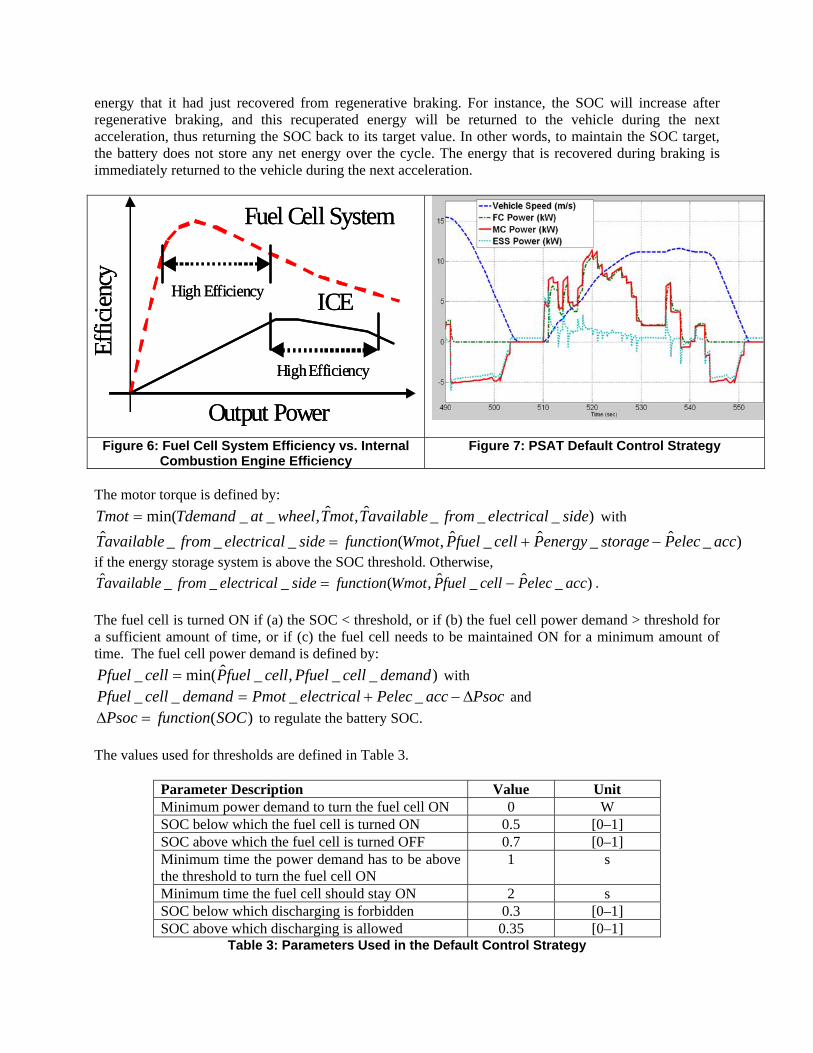
energy that it had just recovered from regenerative braking. For instance, the SOC will increase after regenerative braking, and this recuperated energy will be returned to the vehicle during the next acceleration, thus returning the SOC back to its target value. In other words, to maintain the SOC target, the battery does not store any net energy over the cycle. The energy that is recovered during braking is immediately returned to the vehicle during the next acceleration.

Output Power

Effic

ienc

y

Fuel Cell System

ICEHigh Efficiency

High Efficiency

Output Power

Effic

ienc

y

Fuel Cell System

ICEHigh Efficiency

High Efficiency

Figure 6: Fuel Cell System Efficiency vs. Internal

Combustion Engine EfficiencyFigure 7: PSAT Default Control Strategy

The motor torque is defined by:

)___ˆ,ˆ,__min( sideelectricalfromavailableTmotTwheelatTdemandTmot with

)_ˆ_ˆ_ˆ,(___ˆ accelecPstorageenergyPcellfuelPWmotfunctionsideelectricalfromavailableT if the energy storage system is above the SOC threshold. Otherwise,

)_ˆ_ˆ,(___ˆ accelecPcellfuelPWmotfunctionsideelectricalfromavailableT . The fuel cell is turned ON if (a) the SOC < threshold, or if (b) the fuel cell power demand > threshold for a sufficient amount of time, or if (c) the fuel cell needs to be maintained ON for a minimum amount of time. The fuel cell power demand is defined by:

)__,_ˆmin(_ demandcellPfuelcellfuelPcellPfuel with

PsocaccPelecelectricalPmotdemandcellPfuel ____ and

)(SOCfunctionPsoc to regulate the battery SOC. The values used for thresholds are defined in Table 3.

Parameter Description Value Unit Minimum power demand to turn the fuel cell ON 0 W SOC below which the fuel cell is turned ON 0.5 [0–1] SOC above which the fuel cell is turned OFF 0.7 [0–1] Minimum time the power demand has to be above the threshold to turn the fuel cell ON

1 s

Minimum time the fuel cell should stay ON 2 s SOC below which discharging is forbidden 0.3 [0–1] SOC above which discharging is allowed 0.35 [0–1]

Table 3: Parameters Used in the Default Control Strategy

Figure 8 displays the additional power demand to the fuel cell used to regulate the energy storage system SOC.

Figure 8: Additional Power ( Psoc ) Requested for the SOC Control

To compare the simulation results with the optimized ones, a SOC correction algorithm was used in PSAT. The dichotomy method was selected among several options in PSAT. In this case, the initial SOC is modified until the tolerance (difference between initial and final SOC) is met. To characterize and compare the different strategy performances, their efficiency is computed as the ratio between the PSAT and the optimized fuel economies. For example, for the ECE cycle in Table 4, the default PSAT strategy has a fuel economy of 70.3 mpgge, when the optimized one is 106.8 mpgge, leading to an efficiency of 70.3 / 106.8 = 78.5%. This measure has the advantage to be independent of the strategy types, hypothesizes and parameters. Table 4 compares the fuel economy results between the initial PSAT simulation and the optimized algorithm. PSAT Simulations Optimization algorithm

(mpgge) Efficiency of default

strategy (%) SOC Init (0-1) Default PSAT Strategy (mpgge)

ECE 0.718 70.3 106.8 78.5 NEDC 0.715 77.3 98.5 65.8 HWFET 0.7 88.4 100.1 88.3 UDDS 0.717 79.0 99.9 79.1

Table 4: Comparison between Optimization and PSAT Default Control Strategy

4.2 Controller Implementation

The optimization algorithm provides control patterns similar to those of the default PSAT controller, where the fuel cell is turned ON on the basis of a power demand threshold and the SOC is regulated by asking more or less power to the fuel cell. However, differences appear related to the power demand level. Figure 9 shows that, for high power demand, both controls provide similar results. However, for low power, differences appear, as shown in Figure 10. In this case, the fuel cell is used during steady-state and low vehicle speed for the PSAT default controller. In addition, during higher power demand, the optimization results demonstrate a higher power requested by the fuel cell.

To conclude, (a) the power level threshold used to start the fuel cell should be increased for the default controller and (b) the SOC algorithm should be tightened to request additional power from the fuel cell with in use.

Figure 9: High Power Demand – Part of HWFET Cycle

Figure 10: Low Power Demand – Part of NEDC Cycle

When trying to optimize HEV, one should keep in mind all of the energy sources (in our case, the fuel cell and the battery). On the basis of the optimization results analysis, the first approach used to improve the simulated fuel economy from PSAT involves using different values for the minimum power demand used to turn the fuel cell ON. The results, summarized in Table 5, demonstrate the potential improvements in fuel economy when using a higher value (e.g., 91.2 mppge vs. 88.4 mppge for the 5kW case).

One major issue, however, appears as the initial SOC varies from case to case. Table 2 already has shown that the initial SOC used for the optimization has an impact on fuel economy. As the fuel economy varies with initial SOC, the optimization should be rerun for each value (e.g., SOC = 63.5) to figure out how close the simulated and the optimized fuel economies are for the same SOC. The process then becomes iterative.

Minimum Power demand to turn the fuel cell ON (kW)

Initial SOC Fuel Economy (mpgge)

5 63.5 91.2 10 71.3 88.7 15 71.7 88.1 20 71.7 88.1

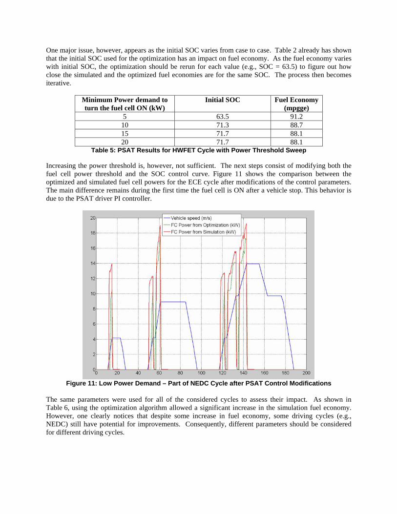
Table 5: PSAT Results for HWFET Cycle with Power Threshold Sweep Increasing the power threshold is, however, not sufficient. The next steps consist of modifying both the fuel cell power threshold and the SOC control curve. Figure 11 shows the comparison between the optimized and simulated fuel cell powers for the ECE cycle after modifications of the control parameters. The main difference remains during the first time the fuel cell is ON after a vehicle stop. This behavior is due to the PSAT driver PI controller.

Figure 11: Low Power Demand – Part of NEDC Cycle after PSAT Control Modifications

The same parameters were used for all of the considered cycles to assess their impact. As shown in Table 6, using the optimization algorithm allowed a significant increase in the simulation fuel economy. However, one clearly notices that despite some increase in fuel economy, some driving cycles (e.g., NEDC) still have potential for improvements. Consequently, different parameters should be considered for different driving cycles.

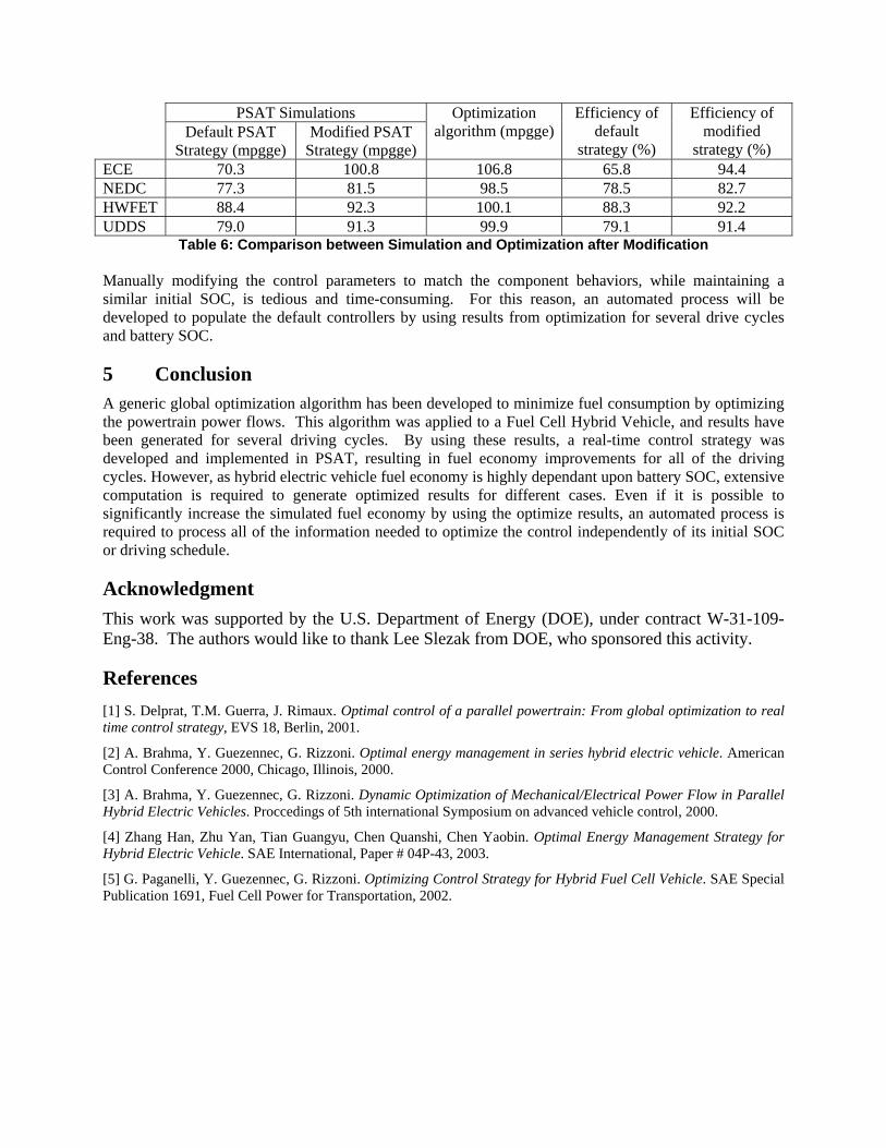
PSAT Simulations Optimization algorithm (mpgge)

Efficiency of default

strategy (%)

Efficiency of modified

strategy (%) Default PSAT

Strategy (mpgge) Modified PSAT

Strategy (mpgge) ECE 70.3 100.8 106.8 65.8 94.4 NEDC 77.3 81.5 98.5 78.5 82.7 HWFET 88.4 92.3 100.1 88.3 92.2 UDDS 79.0 91.3 99.9 79.1 91.4

Table 6: Comparison between Simulation and Optimization after Modification Manually modifying the control parameters to match the component behaviors, while maintaining a similar initial SOC, is tedious and time-consuming. For this reason, an automated process will be developed to populate the default controllers by using results from optimization for several drive cycles and battery SOC.

5 Conclusion A generic global optimization algorithm has been developed to minimize fuel consumption by optimizing the powertrain power flows. This algorithm was applied to a Fuel Cell Hybrid Vehicle, and results have been generated for several driving cycles. By using these results, a real-time control strategy was developed and implemented in PSAT, resulting in fuel economy improvements for all of the driving cycles. However, as hybrid electric vehicle fuel economy is highly dependant upon battery SOC, extensive computation is required to generate optimized results for different cases. Even if it is possible to significantly increase the simulated fuel economy by using the optimize results, an automated process is required to process all of the information needed to optimize the control independently of its initial SOC or driving schedule.

Acknowledgment

This work was supported by the U.S. Department of Energy (DOE), under contract W-31-109-Eng-38. The authors would like to thank Lee Slezak from DOE, who sponsored this activity.

References

[1] S. Delprat, T.M. Guerra, J. Rimaux. Optimal control of a parallel powertrain: From global optimization to real time control strategy, EVS 18, Berlin, 2001.

[2] A. Brahma, Y. Guezennec, G. Rizzoni. Optimal energy management in series hybrid electric vehicle. American Control Conference 2000, Chicago, Illinois, 2000.

[3] A. Brahma, Y. Guezennec, G. Rizzoni. Dynamic Optimization of Mechanical/Electrical Power Flow in Parallel Hybrid Electric Vehicles. Proccedings of 5th international Symposium on advanced vehicle control, 2000.

[4] Zhang Han, Zhu Yan, Tian Guangyu, Chen Quanshi, Chen Yaobin. Optimal Energy Management Strategy for Hybrid Electric Vehicle. SAE International, Paper # 04P-43, 2003.

[5] G. Paganelli, Y. Guezennec, G. Rizzoni. Optimizing Control Strategy for Hybrid Fuel Cell Vehicle. SAE Special Publication 1691, Fuel Cell Power for Transportation, 2002.

Authors

Sylvain Pagerit, Research Engineer, Argonne National Laboratory, 9700 South Cass Avenue, Argonne, IL 60439-4815, USA, spagerit@anl.gov

Sylvain Pagerit received a Master of Science in Industrial Engineering from the Ecole des Mines de Nantes, France, in 2000, as well as a Master of Science in Electrical Engineering from the Georgia Institute of Technology, Atlanta, in 2001. He worked on Hierarchical Intelligent Controller for HEV at the Intelligent Control and System Laboratory of Georgia Tech for 2 years, and he is now working at Argonne National Laboratory on PSAT

Aymeric Rousseau, Research Engineer, Argonne National Laboratory, 9700 South Cass Avenue, Argonne, IL 60439-4815, USA, arousseau@anl.gov Aymeric Rousseau is head of the Advanced Powertrain Vehicles Modeling Department at Argonne National Laboratory. He received his engineering diploma at the Industrial System Engineering School in La Rochelle, France, in 1997. He then received his Technology Research Diploma from La Rochelle University on the basis of his work on Hybrid Electric Vehicles modeling in 1998. After working for PSA Peugeot Citroen for 3 years in the Hybrid Electric Vehicle research department, he joined Argonne National Laboratory, where he is now responsible for the development of PSAT.

Phil Sharer, Research Engineer, Argonne National Laboratory, 9700 South Cass Avenue, Argonne, IL 60439-4815, USA, psharer@anl.gov

Phillip Sharer is Systems Analysis Engineer at Argonne National Laboratory. He received a Master of Science in Engineering from Purdue University Calumet in 2002. He has over five years of experience modeling hybrid electric vehicles, using PSAT at Argonne National Laboratory.