global marine gravity from retracked geosat and ers-1 altimetry

Global marine gravity from retracked Geosat and ERS-1 altimetry:

Ridge segmentation versus spreading rate

David T. Sandwell1 and Walter H. F. Smith2

Received 12 August 2008; revised 20 October 2008; accepted 18 November 2008; published 31 January 2009.

[1] Three approaches are used to reduce the error in the satellite-derived marine gravityanomalies. First, we have retracked the raw waveforms from the ERS-1 and Geosat/GMmissions resulting in improvements in range precision of 40% and 27%, respectively.Second, we have used the recently published EGM2008 global gravity model as areference field to provide a seamless gravity transition from land to ocean. Third, we haveused a biharmonic spline interpolation method to construct residual vertical deflectiongrids. Comparisons between shipboard gravity and the global gravity grid show errorsranging from 2.0 mGal in the Gulf of Mexico to 4.0 mGal in areas with rugged seafloortopography. The largest errors of up to 20 mGal occur on the crests of narrow largeseamounts. The global spreading ridges are well resolved and show variations in ridge axismorphology and segmentation with spreading rate. For rates less than about 60 mm/a thetypical ridge segment is 50–80 km long while it increases dramatically at higher rates(100–1000 km). This transition spreading rate of 60 mm/a also marks the transition fromaxial valley to axial high. We speculate that a single mechanism controls both transitions;candidates include both lithospheric and asthenospheric processes.

Citation: Sandwell, D. T., and W. H. F. Smith (2009), Global marine gravity from retracked Geosat and ERS-1 altimetry: Ridge

segmentation versus spreading rate, J. Geophys. Res., 114, B01411, doi:10.1029/2008JB006008.

1. Introduction

[2] Marine gravity anomalies derived from radar altimetermeasurements of ocean surface slope are the primary datafor investigating global tectonics and continental marginstructure [Cande et al., 2000; Fairhead et al., 2001; Lawveret al., 1992; Laxon and McAdoo, 1994;Mueller et al., 1997].In addition, altimeter-derived gravity has been combinedwith sparse ship soundings to construct global bathymetrygrids [Baudry and Calmant, 1991; Dixon et al., 1983; Jungand Vogt, 1992; Ramillien and Cazenave, 1997; Smith andSandwell, 1994, 1997]. The bathymetry and seafloor rough-ness vary throughout the oceans as a result of numerousgeologic processes [Brown et al., 1998]. This seafloortopography influences the ocean circulation and mixing thatmoderate Earth’s climate [Jayne et al., 2004; Kunze andLlewellyn Smith, 2004; Munk and Wunch, 1998] and thebiological diversity and food resources of the sea.[3] While these satellite altimeter data are enormously

valuable for exploring the remote ocean basins, the amountof geodetically useful data that has been collected iscomparatively small. To date, eight high-precision radaraltimeter missions (Geosat 1985–1989, ERS-1 1991–1998,Topex/Poseidon 1992–2006, ERS-2 1995–present, GFO,

1998–present, Jason 1, 2001–present, ENVISAT 2002–present, and Jason 2 2008–present) have logged 63 years ofsea surface height measurements. However, only a smallfraction (2.4 years or 4%) of these data have spatially denseground tracks that are suitable for gravity field recovery.Most of the 63 years of altimeter data were collected fromthe repeat orbit configuration that is optimal for recoveringchanges in ocean surface height associated with currentsand tides [Fu and Cazenave, 2001]. The only sources ofnonrepeat altimeter data are the geodetic phases of Geosat(18 months) and ERS-1 (11 months). These nonrepeatprofiles, combined with ‘‘stacks’’ (temporal averages) ofrepeat profiles from the other altimeters, have been used innumerous studies to estimate the short wavelengths (<400 km)of the marine gravity field [Andersen and Knudsen, 1998;Cazenave et al., 1996; Hwang and Parsons, 1996; Sandwelland Smith, 1997; Tapley and Kim, 2001]. The longerwavelength gravity field is more accurately measured atorbital altitude using spacecraft such as CHAMP [Reigber etal., 2002], GRACE [Tapley et al., 2005], and GOCE [Kleeset al., 2000].[4] Because of this limited supply of data, the geodetic

community has made every effort to improve the accuracyand resolution of the nonrepeat phases of the Geosat andERS-1 missions. For recovery of the static marine gravityfield, the critical measurement is the slope of the oceansurface. Laplace’s equation combined with Bruns’ formulashows that one microradian (mrad) of ocean surface sloperoughly corresponds to 1 milligal (mGal) of gravity anom-aly [Haxby et al., 1983]. Ocean surface slope can beestimated by differencing height measurements along satel-

JOURNAL OF GEOPHYSICAL RESEARCH, VOL. 114, B01411, doi:10.1029/2008JB006008, 2009ClickHere

for

FullArticle

1Scripps Institution of Oceanography, University of California, SanDiego, La Jolla, California, USA.

2Laboratory for Satellite Altimetry, NOAA, Silver Spring, Maryland,USA.

Copyright 2009 by the American Geophysical Union.0148-0227/09/2008JB006008$09.00

B01411 1 of 18

http://dx.doi.org/10.1029/2008JB006008

lite altimeter profiles so absolute range accuracy is largelyirrelevant [Sandwell, 1984]. Indeed the usual correctionsand ancillary data that are needed to recover the temporalvariations in ocean surface height associated with currentsand eddies are largely unimportant for the recovery of thegravity field because the slope of these corrections is far lessthan the slope error in the radar altitude measurement.[5] One way of improving the range precision of the

altimeter data is to retrack the raw altimeter waveform.Standard waveform retracking estimates three to fiveparameters, the most important being arrival time, risetimeor significant wave height (SWH), and return amplitude[Amarouche et al., 2004; Brown, 1977]. Arrival time andSWH are inherently correlated because of the noise char-acteristics of the return waveform [Maus et al., 1998;Sandwell and Smith, 2005]. Two previous studies havedemonstrated up to 40% improvement in range precisionby optimizing the retracking algorithm to achieve highrange precision at the expense of recovering small spatialscale variations in ocean wave height [Maus et al., 1998;Sandwell and Smith, 2005]. We have retracked the ERS-1altimeter waveform data for all of the geodetic phase andpart of the 35-day-repeat phase, and we have made theseretracked data available to the scientific community. Theseretracked ERS-1 data were used to construct a new marinegravity model for investigating the relationship betweenlinear volcanic chains and 150 km wavelength gravitylineations in the Central South Pacific [Sandwell andFialko, 2004] discovered by Haxby and Weissel [1986].[6] In this study we make three additional improvements

to the accuracy and resolution of the global marine gravityfield. First, we retrack all the altimeter waveforms from theGeosat Geodetic Mission (GM) using a two-step algorithmsimilar to the algorithm we developed for retracking theERS-1 data [Sandwell and Smith, 2005]. Recently, Lillibridgeet al. [2004] have completed a major upgrade of the GMdata by constructing a new Geosat data product. Thisproduct comprises the original sensor data records withthe waveform data records, yielding a complete data set atthe full (10 Hz) sampling rate. This data set includes theoriginal radar range measurements made by the onboard‘‘alpha-beta’’ tracker, and the returned radar power (‘‘wave-forms’’), so that the latter may be reprocessed (‘‘retracked’’)and compared with the former.[7] The second improvement to the global marine gravity

field is to grid the along-track slope data into a consistentsurface using a biharmonic spline interpolation algorithm.Our previous satellite gravity grids [Sandwell and Smith,1997] used an iterative approach [Menke, 1991] to calculatea surface that is consistent with all this slope data. Here weuse a 2-D biharmonic Greens functions approach originallydeveloped by Sandwell [1987] to combine slopes fromnoisy GEOS-3 radar altimeter profiles with more preciseslopes from Seasat profiles. This method has been extendedby Wessel and Bercovici [1998] to also include a tensionparameter which helps to suppress spline overshoots inareas of sharp gradient.[8] Our third improvement is the use of a new global

geopotential model, EGM2008, complete to sphericalharmonic degree 2160, for the remove/restore procedure[Pavlis et al., 2007]. Previously, we used EGM96 [Lemoineet al., 1998] to degree and order 360. The higher spatial

resolution of EGM2008 results in a major improvement ingravity near shorelines. An estimate of the mean oceandynamic topography (MDOT) included with EGM2008corrects a portion of the sea surface slope associated withwestern boundary currents resulting in a 6–10 mGal im-provement in gravity anomaly accuracy in these areas.

2. Data Analysis

2.1. Retracking Altimeter Waveforms

[9] As mentioned above and discussed more fully inseveral previous publications [e.g., Sandwell, 1984; Rummeland Haagmans, 1990; Hwang and Parsons, 1996; Sandwelland Smith, 1997; Andersen and Knudsen, 1998], the accu-racy of the gravity field derived from satellite altimetry isproportional to the accuracy of the local measurement ofocean surface slope. Since the height of the ocean surface ata particular location varies with time because of tides,currents, and atmospheric pressure, the most accurate slopemeasurements are from continuous altimeter profiles. Con-sider the recovery of a 1 mGal accuracy gravity anomalyhaving a wavelength of 28 km. This requires a sea surfaceslope accuracy of 1 microradian (mrad) over a 7 km lengthscale (1 s of flight along the satellite track), necessitating aheight precision of 7 mm in one-per-second measurementsof sea surface height. Current satellite altimeters withstandard onboard waveform tracking such as Geosat,ERS-1/2, and Topex have typical 1-s averaged range preci-sion of 30–40 mm resulting in gravity field accuracies of4–6 mGal.[10] A more serious issue with the onboard waveform

trackers is that they must perform the tracking operation inreal time using a so-called alpha-beta tracking loop. TheGeosat onboard tracker acts as a critically damped oscillatorwith a resonance around 0.4 Hz and a group delay of about0.25 s. Sea surface heights computed from the onboardtracker’s range estimates thus have amplified noise in aband centered around 18 km wavelength, while localextrema in height are displaced about 1.7 km down-trackof their true position. Retracking eliminates the resonanceand the delay, placing features at the proper location alongthe ground track and sharpening the focus on small-scalefeatures.[11] The retracking method employed here is two step:

first, a five-parameter waveform model (Figure 1) is fit toeach 10-Hz waveform, solving for arrival time (to), risetime(s), amplitude (A), prearrival noise floor (N), and trailing-edge plateau decay (k). In the second pass of retracking,along-track smoothed values of all the parameters except therange arrival time, t0, are formed and a one-parameter fit ofthe arrival time is made with the other four parameters set totheir smoothed values. This has the desirable effect ofdecoupling noise in the estimation of range from noise inthe estimation of the risetime.[12] To illustrate the inherent correlation between errors

in estimated arrival time and errors in estimated risetime, weperformed a Monte Carlo experiment simulating modelfitting to noisy data [Sandwell and Smith, 2005]. In theexperiment we generated 2000 realizations of noisy wave-forms, each waveform having the same known true param-eters for arrival time, risetime, and amplitude, plus arealistic power-dependent random noise. We then did a

B01411 SANDWELL AND SMITH: GLOBAL MARINE GRAVITY

2 of 18

B01411

least squares fit to each waveform, obtaining 2000 noisyestimates of each model parameter, and we examined theerror distribution in these estimated parameters. The resultof this simulation (Figure 1b) shows a severe correlationbetween risetime and arrival time having a slope of 1. TheRMS scatter of the estimated arrival time about the truearrival time is 28 mm. If we assume that the risetime variessmoothly along the satellite track because it reflects asmoothly varying field of surface waves and we constrainthe risetime to the smoothed value, then the RMS scatter inthe estimated arrival time is 18 mm, or a 36% reduction inRMS scatter (59% reduction in variance).[13] Improvements due to retracking of Geosat are char-

acterized in terms of both spatial resolution and noise level.The spatial resolution is estimated by analyzing pairs of seasurface height profiles from nearly collinear tracks andperforming a cross-spectral analysis of the height profilepairs, assuming each is a realization of a random processwith coherent signal and incoherent noise [Bendat andPiersol, 1986], as shown in Figure 2. The power spectraof both signal and noise in sea surface height are shown,before and after retracking. The noise power is cut nearly50%, resulting in an improvement in spatial resolution ofnearly 5 km from 29 km to 24 km. These improvementsresult in a noticeable sharpening of seafloor tectonic signals,as well as a reduction in false sea surface height variabilityassociated with increased SWH variability (e.g., in theSouthern Ocean). The crossover point between signal andnoise also indicates that the shortest wavelength resolvable

in an individual Geosat profile is about 24 km in the deepocean.[14] To assess the reduction of noise due to retracking, we

compare sea surface slope along the GEOSAT GM profileswith the slope from our latest gravity model (version 18),presented in section 2.2. Since the model combines data fromboth ascending and descending tracks of Geosat, ERS-1,

Figure 1. (top) Average of 10,000 Geosat radar waveforms (dotted) and a simplified model with fiveadjustable parameters: A, amplitude; to, arrival time; s, risetime; N, leading edge noise floor; k, trailingedge decay. The spacing of the gates is 3.12 ns or 468. mm. (bottom) Error in estimated arrival timeversus error in estimated risetime for a synthetic experiment using realistic waveform data. The RMSerror in arrival time is 28.4 for the unconstrained solution and 18.1 mm when the risetime was fixed.

Figure 2. Power spectrum of sea surface height before(gray) and after (black) retracking. Noise spectra are dashedwhile signal spectra are solid. Retracking cuts noise powerby 50% at mesoscale and shorter wavelengths. The spatialresolution is also increased, since the signal power remainsabove the noise power to shorter wavelengths.


3 of 18

B01411

and Topex, the comparison between model slopes andGeosat track slopes is not entirely circular thinking, and itillustrates clearly the improvements due to retracking.Figure 3 shows the RMS difference between along-trackslope from Geosat GM and the corresponding slope fromnorth and east vertical deflection grid products averaged at2 min resolution. The difference profiles are low-passfiltered with a Gaussian filter having a 0.5 gain at wave-lengths of 18 km (Figure 3, top and middle) and 80 km(Figure 3, bottom). The RMS of the differences, averaged in0.25� cells, is displayed in Figure 3. The upper RMSdifference map uses the original Geosat GM product trackedby the onboard a-b tracker [Lillibridge and Cheney, 1997]sampled at 5 Hz along track. The overall RMS difference is4.4 mrad. The map shows three categories/areas where theRMS differences exceed the background value (�2 mrad).First, there are latitudinal bands of high noise especiallybetween 30� and 60� south latitude. This noise is primarilydue to ranging from a surface that is roughened by highwaves due to storms and high wind. The second type ofhigh noise area is associated with areas of very high seasurface slope near large seamounts, fracture zones, andspreading ridges. This noise is primarily due to the 1.7 kmphase shift of the onboard tracker which causes a misalign-ment of the sharp feature with the feature recovered in theprofile. The third type of noise is due to mesoscale varia-tions in sea surface slope associated with eddies andmeandering currents [Cheney et al., 1983].[15] Figure 3 (middle) shows the same comparison but

after retracking the Geosat GM waveforms. The overallRMS difference is reduced to 3.2 mrad which corresponds toa 27% improvement in RMS (47% in variance). Note thenoise due to the rough ocean surface is dramaticallyreduced. Also differences associated with very high seasurface slope are mostly gone. These two reductions innoise are due to the retracking which reduces the sensitivityof the range due to ocean waves and also corrects the phaseshift from the onboard tracker. Unfortunately, the ‘‘noise’’due to mesoscale ocean variability remains. Indeed addi-tional smoothing of the slope differences along track(Figure 3, bottom) further highlights the spatial variationsin slope variability and the association of areas of highervariability with deeper [Sandwell and Zhang, 1989] andsmoother [Gille et al., 2000] seafloor. Assuming that theRMS differences at wavelengths longer than 80 km are alldue to ocean processes, one can estimate the slope error dueto ranging noise as 2.8 mrad, which corresponds to 2.8 mGal.Below we will confirm this noise level through a compar-ison with shipboard gravity measurements.

2.2. Geoid Slope and Gravity Anomaly ModelConstruction

[16] The marine gravity field model was constructed asdescribed in our previous publication [Sandwell and Smith,

1997] but with the following improvements. The grid cellsize was reduced from 2 min to 1 min in an effort to retainhigher spatial resolution. The latitude range was extendedfrom ±72� to ±80.7� to recover more gravity information inthe polar regions. This results in a grid of 2-byte integerswith 21,600 columns and 17,280 rows. Our model uses a‘‘remove-restore’’ procedure to blend short-wavelength de-tail from satellite altimetry with the large-scale anomalies ofgeopotential models; in 1997 we used the EGM96 model(complete to degree 360, or 110 km wavelength), while wenow use the EGM2008 geoid height model complete todegree and order 2160 including the matching EGM2008mean dynamic ocean topography (MDOT) model. In thefinal iteration we also high-pass filter the residual slopes(0.5 gain at 180 km wavelength) to further reduce theinfluence of unmodeled dynamic ocean topography or tides.The short-wavelength detail is obtained by gridding theresidual sea surface slopes along altimeter tracks. In ournew model we use more data than in 1997, includingretracked data, and we combine the data in a new way,using biharmonic splines with a tension parameter of 0.25as described by Wessel and Bercovici [1998].[17] There are two major tasks in our data modeling

process. The first task is to build a seamless model of theglobal marine geoid slope, that is, the north and eastcomponents of the deflection of the vertical, by incorporat-ing all available altimeter data and removing the sea surfaceslope component due to dynamic ocean signals such astides, mesoscale currents, and their eddies. The second taskis to take the geoid slopes obtained in task one and convertthem to gravity anomalies. Only in this second task do weemploy a gravity field model, such as EGM96 orEGM2008. Our data modeling process produces modelsof geoid slope as well as gravity anomalies.[18] To begin the modeling of geoid slope, we remove the

UT CSR 4.0 tide model [Bettadpur and Eanes, 1994] fromeach altimeter profile’s sequence of height samples taken atthe highest available data rate (10 Hz or 20 Hz, dependingon the satellite). The data are low-pass filtered with a cutthat begins at 26.8 km wavelength, has 0.5 gain at 14.6 km,and zeros at 10 km; this filter was designed in Matlab usingthe Parks-McClellan algorithm. After this filter is appliedthe data can be downsampled to a 5 Hz sampling rate,which corresponds to an along-track spacing of 1.4 km.Because the data in the stacks of GEOSAT ERM and TOPEXwere acquired with the onboard tracker, we applied anadditional filter to these stacked data to undo (as much aspossible) the along-track phase shift and group delay asso-ciated with the onboard tracker as described by W. H. F.Smith and D. T. Sandwell (manuscript in preparation,2009). After this initial filtering we have sea surface heightdata from all seven data sources in the same form, with thesame sampling rate and without phase shifts.

Figure 3. (top) RMS deviation of along-track slopes from the Geosat GM data from onboard tracking with respect toslopes derived from our best estimate of the gravity field (this paper). The global RMS variation is 4.4 mrad. (middle) RMSdeviation of along-track slopes from retracked Geosat GM data with respect to slopes derived from our best estimate of thegravity field has a global RMS of 3.19 mrad or a 27% improvement. (bottom) Along-track slope differences (retracked) butlow-pass filtered at 80 km wavelength. This RMS deviation of 1.56 mrad is mostly real signal due to mesoscale variations inocean surface slope.


4 of 18

B01411

Figure 3


5 of 18

B01411

[19] The along-track sea surface slope of each profile isthen computed and compared to our prior models of geoidslope, for two reasons. First, the prior model furnishes asanity check that allows us to detect outliers that producespurious slopes. Our edit threshold was set at three timesthe standard deviation given in Table 1. Second, we filter(0.5 gain at 180 km wavelength) the differences in slopebetween the profile and the model to remove long-wavelengthprofile slope components due to unmodeled tides, currents,and eddies. After these steps the remaining sea surface slopedata are presumed to measure geoid slope, that is, deflectionof the vertical. Verification that this is the case comes afterthe geoid slopes have been converted to gravity anomalies,when we can compare these gravity anomalies to thosemeasured by ships carrying gravimeters.[20] The conversion of vertical deflections to gravity

anomalies is a boundary-value problem for Laplace’s equa-tion. The most accurate computations use spherical harmon-ics at long wavelengths, supplemented by Fouriertransforms on data conformally projected onto a flat planefor short wavelengths. We follow a standard practice ingeodesy known as a ‘‘remove-restore procedure’’: a spher-ical harmonic model such as EGM96 or EGM2008 fur-nishes long-wavelength deflections and gravity anomalies,the deflections are removed from our data, the residualdeflections are converted to residual gravity anomalies byFourier transform, the residual anomalies are then added tothe spherical harmonic model anomalies to obtain the totalanomaly field.[21] It is important to understand that use of this proce-

dure does not imply that our model exactly matches thespherical harmonic model at all wavelengths contained inthe spherical harmonic model. In principle, if our datadisagree with the EGM model at any wavelength, thenthere will be power in our residual at that wavelength, andso our data may be used to improve the model at allwavelengths. In practice, however, the Fourier transformcalculation must be confined to a limited range of latitudeswhere the conformal projection has a limited range ofscales, so that the flat-earth approximation is valid, and thislimits the longest wavelengths (�650 km) at which thealtimeter data may influence the model. Common practicein geodesy uses ‘‘least squares collocation’’ to model theresidual anomalies and usually assumes that the mean valueof the residual anomaly will be zero. We find it convenient

to assume that the mean anomaly is small over a patch areafor calculating the best spline fit to the seven altimeter datasources, as discussed below.[22] Our models ‘‘feel’’ the influence of the spherical

harmonic model most strongly near shorelines. The altim-eter data cannot furnish information about the geoid slopeover land, and our residual slopes taper smoothly to zero inland areas. The Laplace boundary value problem is solvedas a convolution, so that the gravity anomaly at a pointdepends on deflections in a region around that point. Ourprior models used EGM96, which furnished information toharmonic degree 360, or about 100 km wavelength, and soour solutions began to degrade as one moved closer to shorethan 50 km. Our latest solutions use EGM2008, complete todegree 2160, or about 19 km wavelength, so our solutionsshould feel the lack of land data only about 10 km fromshore.[23] Our model development actually involved two iter-

ations and interactions with the group developing EGM2008[Pavlis et al., 2008]. First, we constructed a gravity modelV16.1 combining all our retracked altimetry and the sevensources of data, but using the EGM96, complete to degreeand order 360, as a reference field. The largest source oferror in our V16.1 gravity grids is within 50 km of shore[Maia, 2006] because of the zeros on land in the residualdeflection data. We hoped the group developing EGM2008might use our deflections at sea; however, they preferred touse the gravity anomalies from our V16.1 field. These oceandata were combined with land and shipboard gravity data aswell as longer-wavelength (>400 km) satellite gravityinformation to construct a new global reference field com-plete to degree and order 2160 called EGM2007b. TheEGM team provided us with this new model, which we thenused in our remove/restore procedure to construct a secondmarine gravity model called V17.1. Because this modelincluded more complete land gravity information during theslope-to-gravity conversion, the errors in nearshore areaswere presumably reduced. To reiterate, our north and eastdeflection grids from version 16.1 and 17.1 are identical;only the gravity models are different and the differences aresmall except near shorelines. The EGM team then used theV17.1 gravity model in the final construction of EGM2008.Close to the shorelines, the land data available in EGM2008improves the accuracy of our nearshore marine gravityanomalies.[24] An additional improvement in our version 18.1 over

our version 17.1 comes from the EGM2008 mean dynamictopography model. For version 18.1 we removed the slopeof this model from our deflections. The slope of the meandynamic ocean topography is negligible except wherewestern boundary currents that produce large ocean surfaceslopes (1–10 mrad) remain spatially fixed over time.[25] All of these fields (V16–18) use the same along-

track altimeter slopes derived from seven data sources asdescribed in Table 1 in their order of importance. Almost allof the gravity information comes from the retracked profilesof the GEOSAT GM and ERS-1 GM. Nevertheless the otherdata sets provide targeted new information. For example,the 501 tracks of the ERS-1 exact repeat mission (ERM)provide significant new information at high latitudes wherethe tracks converge and the stacking of multiple cyclesprovides coverage in ice-free times. The TOPEX ERM data

Table 1. Summary of Slope Data and A Priori Uncertainties Used

for Gravity Model Constructiona

Number ofObservations

(106)Uncertainty

(mrad)

GEOSAT GM 125 8.2ERS-1 GM 111 9.7ERS-1 ERM (35-day repeat) 9.2 4.7GEOSAT ERM (17 day repeat) 4.8 7.5TOPEX ERM (10 day repeat) 2.8 4.5TOPEX (maneuver) 20 12.6ERS GM - polar (threshold retrack) 9.6 30.

aNote that these 5 Hz data have minimal along-track filtering (0.5 gain at9 km wavelength), whereas the low-pass filter applied for the noise analysisshown in Figure 3 was 18 km.


6 of 18

B01411

provide minimal new information along 127 tracks. How-ever, during September of 2002 the TOPEX track wasmaneuvered to bisect the original 127 tracks. These data,which we call TOPEX maneuver, provide some new infor-mation although we show below that the noise level of thedata is significantly higher than GEOSAT GM data. Finallywe have included some ERSGMdata at high latitudes (>65�)that were retracked using a simple threshold retracker. Thisretracker is able to provide sensible range estimates in icecovered areas where the three-parameter ocean waveformretracker fails. However, these data are extremely noisy andare given very high uncertainty in the least squares estima-tion process (Table 1).[26] Prior to filtering, the along-track slope profiles were

compared with a previous model to detect and edit outliers;the edit threshold was set at 3 times the standard deviationgiven in Table 1. Along-track slopes from the EGM2008geoid plus MDOT model [Pavlis et al., 2008] were removedand the residuals were gridded using a biharmonic splineapproach discussed next.[27] Consider N estimates of slope s(xi) with direction ni

each having uncertainty si. We wish to find the ‘‘smooth-est’’ surface w(x) that is consistent with this set of data suchthat si = (rw . n)i. As in many previous publications wedevelop a smooth model using a thin elastic plate that issubjected to vertical point loads [Briggs, 1974; Smith andWessel, 1990]. The loads are located at the locations of thedata constraints (knots) and their amplitudes are adjusted tomatch the observed slopes [Sandwell, 1987]. To suppressovershooting oscillations of the plate, tension can be appliedto its perimeter. Wessel and Bercovici [1998] solved thisproblem by first determining the Greens function for thedeflection of a thin elastic plate in tension. The differentialequation is

a2r4f xð Þ � r2f xð Þ ¼ d xð Þ ð1Þ

where a is a length scale factor that controls the importanceof the tension. High a results in biharmonic splineinterpolation which minimizes the strain energy in the platebut can produce undesirable oscillations between datapoints [Sandwell, 1987]. Zero a results in harmonicinterpolation, which results in a surface that has sharp localperturbations at the locations of the data constraints. Thetension factor controls the shape of the interpolating surface.Through experimentation we find good-looking resultswhen the solution is about 0.33 of the way from thebiharmonic to the harmonic end-member. The Greensfunction for this differential operator is

f xð Þ ¼ Ko

xj ja

� �þ log

xj ja

� �ð2Þ

where Ko is the modified Bessel function of the second kindand order zero. The smooth surface is a linear combinationof these Greens functions each centered at the location ofthe data constraint.

w xð Þ ¼XNj¼1

cjf x� xj� �

ð3Þ

The coefficients cj represent the strength of each point loadapplied to the thin elastic plate. They are found by solvingthe following linear system of equations.

si ¼ rw nð Þi¼XNj¼1

cjrf xi � xj� �

ni i ¼ 1;N ð4Þ

One issue that must be addressed is the possibility of havingtwo data constraints in exactly (or nearly) the same location.This causes the linear system to be exactly singular (ornumerically unstable) [Sandwell, 1987]. Our satellitealtimeter data commonly have many crossing profiles so itis possible to have two or even six slope constraints atnearly the same location. The solution to this problem is toreduce the number of Greens functions (knots) by makingsure they are not more closely spaced than some prescribeddistance. That minimum distance should be about 1/4 ofthe shortest wavelength that one hopes to resolve. Whenthe number of knot locations is less than the number ofconstraints then the linear system is overdetermined and thesurface will not exactly match the slope constraints. Sincewe only wish to match the slopes to within the expecteduncertainty of each data type, each equation (4) should bedivided by the slope uncertainty to provide the optimalsolution using a singular value decomposition algorithm. Inour case we are not interested in the absolute height of thesurface but just the local slope so our final result is thegradient of the surface.

rw xð Þ ¼XNj¼1

cjrf x� xj� �

ð5Þ

While this interpolation theory is elegant and very flexible,it is difficult to apply to the altimeter interpolation problembecause there are over 200 million observations to grid(Table 1). Consider gridding just 1000 slopes, the matrix ofthe linear system in equation (4) could have 106 elements ifall the knot points were retained. In practice we make thefollowing compromises in order to grid this large anddiverse set of data.[28] 1. The data are residuals with respect to the

EGM2008 model so we can assemble and grid the data inoverlapping small areas. We expect the residuals will onlyhave signal at wavelengths of less than 37 km. Therefore fora 1-min Mercator grid at 70� latitude we use a subarea sizeof 64 64 points, which has a dimension of 40 km (120 kmat the equator).[29] 2. To avoid edge effects, the subareas have 100%

overlap and only the inner 32 32 interpolated cells areretained. The global analysis has 675 539 subareas.[30] 3. The along-track slope data from each of the six

possible slope directions (i.e., ascending and descendingprofiles from three satellite inclinations ERS, GEOSAT, andTOPEX) and associated uncertainties are binned onto theregularly spaced 1 min Mercator grid, and only the medianslope of each type is retained for fitting. At midlatitudes thereare typically 2000–3000 slope constraints/uncertainties persubarea and typically 800 unique knot points. The originaldistribution of knot points matches the satellite tracks so thespacing at the equator can be as small as 1.8 km. We further


7 of 18

B01411

reduce the knot spacing to a minimum of 3 min (5.4 km)which seems to be sufficient to capture all the residualsignal for wavelengths >14 km. Since gridding is performedin subareas, the computation time is inversely proportionalto the number of CPUs available. This analysis takes abouta day of computer time when four processors are used. Theresults of the computations are grids of residual east andnorth vertical deflection that are converted to gravityanomalies and vertical gravity gradient as described in ourprevious publication [Sandwell and Smith, 1997]. All gridsare finally low-pass filtered using a filter with a 0.5 gain at16 km, which is close to the cutoff wavelength of the 14.6 kmlow-pass filter that was applied to the profiles. The combi-nation of the two filters has a cutoff wavelength of about20 km which provides good looking results that also havelow RMS misfit to ground truth gravity anomalies collectedby ships. One practical limitation of the current set ofaltimeter data is that a typical track spacing at the equatoris 5 km so one cannot expect to recover wavelengths muchshorter than 20 km.

3. Results

3.1. Gravity Accuracy

[31] The resulting vertical deflection and gravity anomalygrids are evaluated using two techniques. First, we examinethe rms misfit between the model and the along-track slopesfrom each of the seven data types. This analysis is good forexamining the relative contributions of each of the datatypes as well as to examine spatial variations in rms misfit.The second analysis compares the model gravity anomaliesto gravity anomalies collected by ships. This comparisonprovides a more independent assessment of data accuracyand resolution but is limited to a few small areas wherehigh-quality shipboard data are available. Indeed, Maia[2006] has performed a blind test of an earlier version ofthis gravity grid (V16.1 EGM96 was used as EGM2008 wasnot available) and we present a summary of those findingsbelow.[32] The profile versus model evaluations are provided in

Table 2 and Figure 4. Each of the three altimeters has datacollected in the exact repeat mission (ERM) configurationas well as the nonrepeat geodetic mission (GM) configura-tion. For example, 66 repeat cycles of GEOSAT (onboard

tracker) were stacked to form a single GEOSAT ERMprofile. The rms deviation is 2.2 mrad for wavelengthsgreater than 18 km and 1.2 mrad for wavelengths greaterthan 80 km. The nonstacked GEOSAT GM data have higherRMS difference of 3.2 and 1.6 mrad, respectively. The mainfeatures that can be summarized from this analysis are thatthe retracked GM data have an rms noise level of between3.2 and 3.6 mrad for wavelengths greater than 18 km. Thestacked ERM profiles all have a lower noise level depend-ing approximately on the number of repeat cycles stacked.The noise floor of about 1 mrad is due to a combination oferrors such as summarized in Table 3. These estimates oferror are maximum values based on independent analysesand, in general, we find the measured noise for wavelengthsgreater than 80 km to be less than these estimates.[33] The maps of rms difference shown in Figure 4

(western hemisphere only) reveal the spatial variations inthe altimeter noise. The differences from the ERM profiles(maps in left column) are generally less than 1 mrad. Higherrms difference occurs in areas of steep geoid gradientperhaps reflecting the fact that these data were assembledfrom onboard tracked profiles so the inverse alpha-betatracker described above does not completely undo theadverse effects of this causal filter. As expected the ERMprofiles do not show high RMS differences in the areas ofthe western boundary currents because both the model andstacked profile represent the long-term average slope acrossthese features. The rms differences of the GM profiles(maps in right column) are generally higher and, asexpected, show the time variable effects of the westernboundary currents. One step in the slope profile preparationbriefly mentioned above is that, prior to regridding, theresidual slopes were high-pass filtered using a filter with a0.5 gain at 180 km wavelength. This filter was designed toremove the time-varying slopes from the GM profilesmainly associated with mesoscale eddies. All the rmsdifference maps show large differences in areas of seasonaland especially permanent ice cover. These large differencesare due to a combination of errors in the model and theprofiles. The gravity anomalies in these areas will also benoisy. A more careful retracking of the data in the ice-covered areas can provide significant improvements ingravity anomaly accuracy [Laxon and McAdoo, 1994;McAdoo and Laxon, 1997].

Figure 4. RMS differences between the along-track slope from altimeter profiles and the new gravity model averagedfrom 1 min to 2 min resolution. Differences were further filtered with a Gaussian filter having a 0.5 gain at 18 km. Thestacked profiles from the exact repeat missions (left column) have lower noise than the geodetic missions.

Table 2. RMS Altimeter Noise From A Posteriori Comparison With V18 Gravity Modela

Tracker

GEOSAT ERS-1 TOPEX

GMOnboard

GMRetrack

ERMOnboardStack

GMRetrackOcean

GMRetrackIce

ERMStack

ManeuverOnboard

ERMOnboardStack

l > 18 km a 4.45 3.21 2.18 3.57 8.62 1.75 3.34 1.17d 4.36 3.17 2.21 3.55 8.92 1.76 3.33 1.19

l > 80 km a 1.88 1.56 1.15 1.63 2.98 1.02 1.50 0.73d 1.85 1.55 1.15 1.62 3.16 1.02 1.50 0.74

aAltimeter noise is measured in mrad. Values in bold represent ascending (a) and descending (d) data used in gravity model construction.


8 of 18

B01411

Figure 4


9 of 18

B01411

[34] We compare shipboard profiles with three gravitymodels to demonstrate the improvements in resolution andaccuracy due to retracking and the secondary biharmonicinterpolation. The three gravity models are: V9.1 which isbased on all the same data used in this paper but both theERS-1 and GEOSAT GM data are from the originaldistribution of geophysical data records; V11.1 is likeV9.1 but incorporates retracked ERS-1 data [Sandwell andSmith, 2005]; and V18.1 (this paper) which has retrackedERS-1, Geosat GM and also uses the biharmonic interpo-lation as well as the EGM2008 reference model. First it isinstructive to show a visual comparison between the threemodels (Figures 5 and 6). The illuminated gravity anomalymaps for the three cases shows a general decrease in noiselevel moving from V9.1 to V11.1 and finally to V18.1. Thedecrease in noise enables one to identify small-scale fea-tures such as the small gravity high along the axis of theEast Pacific Rise (Figure 5) as well as a field of smalluncharted seamounts southwest of the Galapagos Islands(red oval in Figure 5). New features are apparent in V18.1on the continental margin of South America and the Falk-land Plateau (Figure 6). The dramatic improvement in theresolution of the on-land anomalies is due to EGM2008replacing EGM96.[35] A comparison between the three gravity models and

shipboard gravity measurements provides a more quantita-tive assessment of the accuracy of the gravity models. Thefirst example is a west to east trending ship track in theshallow ocean between Indonesia and Borneo (Figure 7).This is a challenging area for gravity field recovery becausethe altimetry tracks run mainly N–S and the track spacing isgreatest at the equator (�5 km). The gravity anomalies have

relatively short wavelength and low amplitude in relation tothe noise. There is a large mean difference between the shipand altimeter-derived gravity that is probably due to aninaccurate gravity tie value in one of the ports [Wessel andWatts, 1988]. The RMS difference shows an improvementfrom 5.6 mGal for V9.1 to 4.8 mGal for V11.1 to 3.03 mGalfor V18.1. The overall improvement due to retracking andspline interpolation is 46%. The second example is from a200 km by 150 km area in the Gulf of Mexico that has beensurveyed to submilligal accuracy by EDCON Co (Figure 8).The RMS difference is 3.03 mGal V9.1, 3.26 mGal V11.1and 2.03 mGal V15.1. This is a 33% improvement inaccuracy.[36] The third example is from the continental margin

area along the east coast of North America (Figure 9). Thisis a challenging area because the Gulf Stream flows steadilyalong the east side of the continental margin. This introdu-ces a 5–10 mrad slope in the ocean surface that should notbe attributed to a gravity anomaly. In all versions of ourgravity field prior to V18, there is a 5–10 mGal error in thegravity along this current. The EGM2008 geoid model alsoincludes a mean dynamic ocean topography (MDOT) modelhaving a resolution of about 200 km wavelength. We addedthis MDOT to the EGM2008 geoid prior to removing thisfrom the along-track slopes. The false gravity associatedwith the DOT was not restored in the V18.1 gravity modelso the DOT error is minimized. This improvement can beseen through a comparison of a shipboard profile thatcrosses the continental margin and Gulf Stream severaltimes. The longer wavelength error is reduced from 3.14mGal to 1.89 mGal. The remaining error is probablyassociated with inaccurate Eotvos correction for the shipgravity profile which was collected in 1977 prior to GPSnavigation [Wessel and Watts, 1988]. We have performednumerous comparisons with shipboard profiles and alwaysarrive at about the same rms difference of 2.5 to 3.5 mGal.[37] In addition to our in-house comparisons with ship-

board gravity we delivered V16.1 of the grid to MarciaMaia at IFREMER to perform some comparisons usingshipboard gravity data that were still on proprietary hold[Maia, 2006]. Comparisons were performed in two areas,one in the central South Pacific over the FoundationSeamount Chain and a second in the Gulf of Aden. Themain findings are that satellite gravity models underestimatethe short-wavelength, high-amplitude anomalies (e.g., atsubmarine volcanoes). A more complete analysis of thegravity field above sharp seamounts confirms this lack ofresolution [Marks and Smith, 2007]. The quantitative resultsfrom the Maia [2006] study are provided in Table 4. Theraw shipboard gravity contains short wavelength noise atwavelengths shorter than about 10–20 km. When theshipboard data are filtered the RMS differences are between1.8 and 3.5 mGal with a mean RMS difference of 2.7 mGal.

3.2. Ridge Segmentation Versus Spreading Rate

[38] The improved resolution offered by the new globalgravity grid and a matching 1-min bathymetry grid dis-cussed in a related publication (Smith and Sandwell, man-uscript in preparation, 2009) will be useful for investigatingsmall-scale tectonic processes. For example, these improvedresolution grids provide a clearer image of the segmentationof the global spreading ridge. An example of the vertical

Table 3. Estimated Maximum Error in Sea Surface Slope

Signal or Error Source Length (km) Height (cm)Slope(mrad)

Gravity signal 12–400 1–300 1–300Orbit errorsa 8000–20,000 400–1000 <0.5Ionosphereb,c >900 20 <0.22Wet troposphered >100 3–6 <0.6Sea-state biase >20 <0.6 <0.3Inverse barometerf >250 <5 <0.2Basin-scale circulation (steady)g >1000 100 <1El Nino, interannual variability,planetary wavesh

>1000 20 <0.2

Deep ocean tide model errorsd,i >1000 3 <0.03Coastal tide model errorsc,i 50–100 <13 <2.6Eddys and mesoscale variabilityj 60–200 30–50 2.5–5Meandering jet (Gulf Stream)g 100–300 30–100 3–10Steady jet (Florida Current)g 100 50–100 5–10

aDynamic orbit determination using the ISS SIGI system, consideringerrors in force, measurement, attitude, center of mass, and effect ofEXPRESS nadir pallet moment arm. This is a worst case error estimatefrom the ‘‘ABYSS’’ proposal to use the International Space Station. Mostsatellite altimeters are smaller, simpler in shape, and in higher orbits, allfactors which reduce the orbit error [Shum et al., 2009].

b[Imel, 1994].c[Yale, 1997].d[Chelton et al., 2001].e[Monaldo, 1988].f[Ponte, 1994].g[Fu and Chelton, 2001].h[Picaut and Busalacchi, 2001].i[Shum et al., 2001].j[Le-Traon and Morrow, 2001].


10 of 18

B01411

Figure 5. (top) Shaded gravity anomaly for a large region in the Central Pacific Ocean centered at theGalapagos Triple Junction (latitude 11� to �8�, longitude 255� to 270�). Colors saturate at ±60 mGal.The visual noise level decreases as one moves from V9.1 (left) to V11.1 (center) to V18.1 (right). Theaxis of the East Pacific Rise is well defined in V18.1 but more difficult to trace in V9.1 because of thehigher noise level. The red oval outlines a patch of small uncharted seamounts not apparent in V9.1.(bottom) Vertical gravity gradient, or curvature of the geoid, for the same region.

Figure 6. Shaded gravity anomaly for a large region in the South Atlantic centered at the FalklandBasin (latitude �57� to �27�, longitude 294� to 318�). Colors saturate at ±80 mGal. The visual noiselevel decreases as one moves from V9.1 (left) to V11.1 (center) to V18.1 (right). Small-scale gravitystructure is visually apparent in V18.1 but hidden in the higher noise of V9.1. Note also the NW-trendingstriped noise in V11.1 that is largely absent in V18.1. This noise is due to mesoscale ocean variabilitywhich has been suppressed by the additional high-pass filter (180 km wavelength) used in V18.1.


11 of 18

B01411

gravity gradient used as shading on the new global bathym-etry grid at 1 min resolution (Figure 10) helps to delineatethe first- and second-order segmentation of the mid-oceanridges [Macdonald et al., 1988]. A recent study of residualmantle Bouguer anomaly by Gregg et al. [2007] using thisnew V16.1 gravity grid reveals the spreading dependence ofgravity anomalies along oceanic transform faults. Theirstudy combined with previous investigations on the varia-tions in ridge-axis morphology with spreading rate[Menard, 1967; Small, 1994], variations in abyssal hillmorphology/seafloor roughness with spreading rate [Goff,1991; Goff et al., 2004; Small and Sandwell, 1992; Smith,1998], and the order of magnitude variations in seismicmoment release with spreading rate [Bird et al., 2002]highlight the importance of spreading rate in lithosphericstrength and crustal structure. This is a first-order aspect ofplate tectonics that deserves a more comprehensive analysis.[39] A more poorly understood phenomenon is the vari-

ation in ridge segmentation with spreading rate [Abbott,1986; Sandwell, 1986]. A variety of models have beenproposed [Kastens, 1987] for ridge segmentation including:thermal contraction joints [Collette, 1974; Sandwell, 1986],thermal bending stresses [Turcotte, 1974], segmented man-

tle upwellings [Lin and Phipps Morgan, 1992; Magde andSparks, 1997; Parmentier and Phipps Morgan, 1990;Schouten et al., 1985], and minimum energy and damagerheology configurations [Hieronymus, 2004; Lachenbruch,1973; Oldenburg and Brune, 1975]. Following the discov-ery of transform faults more than 40 years ago, there is stillno consensus on why they exist and why the ridge seg-mentation varies with spreading rate. A leading hypothesisis that transform faults and fracture zones provide a mech-anism for ridge-parallel shrinkage of the lithosphere. How-ever, if this is correct then this mechanism should not beeffective on faster spreading ridges where the transformspacing is large. Perhaps other types of cracking and platebending occur along the fast spreading ridges [Gans et al.,2003; Sandwell and Fialko, 2004]. If the plates do notshrink in the ridge-parallel direction then large cracks maypenetrate 30 km deep into the lithosphere as proposed byKorenaga [2007]. Another possibility is that plates readilycontract in all three dimensions. In this case the lateralshrinkage will appear as significant perturbations to theglobal plate motion models [Kumar and Gordon, 2009].[40] We have begun a more careful analysis of on-ridge

and off-ridge segmentation to help resolve these fundamen-

Figure 7. Comparison between satellite-derived gravity models (thin lines) and a shipboard gravityprofile (points) across the Java Sea. (top) Gravity model version 9.1 does not use retracked altimeter dataand has an RMS misfit of 5.62 mGal. The mean difference of 25 mGal is due to a mean error commonlyfound in shipboard gravity [Wessel and Watts, 1988]. (middle) Gravity model version 11.1 uses retrackedERS-1 altimeter data but the Geosat data were not retracked; the RMS misfit is improved by nearly 1to 4.75 mGal. (bottom) Gravity model version 18.1 is based on both retracked ERS-1 and Geosataltimeter profiles and also used the biharmonic spline interpolation method. The RMS is improved furtherto 3.03 mGal, which is a 46% reduction in rms.


12 of 18

B01411

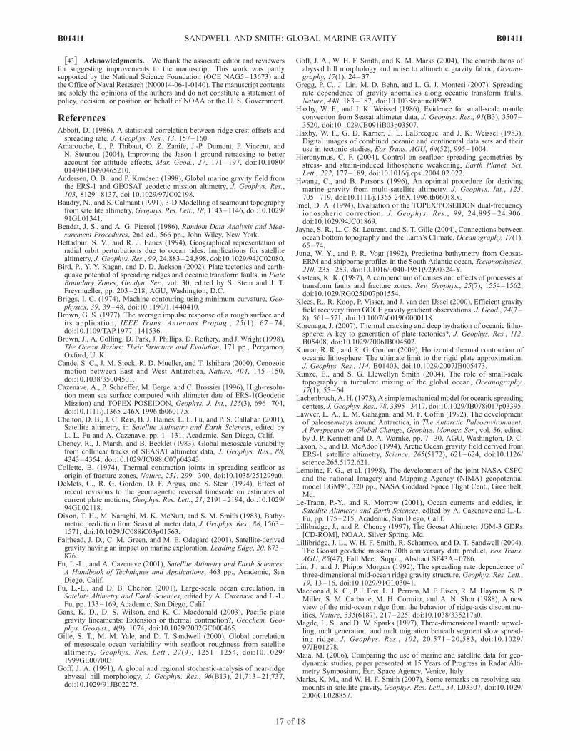
tal issues related to cooling of the oceanic lithosphere.Preliminary results are shown in Figures 11 and 12 wherewe have digitized the first- and second-order discontinuitiesin the global spreading ridge and display the segmentlengths as a function of present-day full spreading rate.The ridges not showing a clear orthogonal pattern of ridgesand transforms at this resolution were not analyzed. Theseinclude the Reykjanes ridge and the northwest end of theSouthwest Indian ridge and the area around the Easter andJuan Fernandez microplates. These preliminary results showa systematic increase in ridge segment length with spread-ing rate although the relationship is not linear. The graycurve is a Gaussian moving average of the data with a sigmaof 20 mm/a. There a change in ridge segment length versusspreading rate that is in accordance with the abrupt changein axial valley topography and gravity anomaly with

spreading rate [Small and Sandwell, 1994]. Because thetransitions occur at the same intermediate spreading rate, itis likely that a single lithospheric or mantle upwellingmechanism controls both processes. A better understandingof ridge segmentation will require a more complete analysisof both ridge axis and ridge flank data that is now availablefrom our new gravity model.

4. Conclusions

[41] Satellite altimetry has provided the most comprehen-sive images of the gravity field of the ocean basins withaccuracies and resolution approaching typical shipboardgravity data. While many satellite altimeter missions havebeen flown over the past 3 decades, only 4% of these datahave nonrepeat orbital tracks that are necessary for gravity

Figure 8. At the bottom right is shown a gravity anomaly map (5 mGal contours) derived from denseshipboard surveys and believed to have submilligal relative accuracy. Also shown are regression plots ofsatellite gravity versus ship gravity with RMS differences of 3.68 mGal for V9.1, 3.26 mGal for version11.1, and 2.03 mGal for version 18.1.

Figure 9. The map shows gravity anomaly (V18.1, contour interval 10 mGal) of area offshore the east coast of NorthAmerica where the Gulf Stream follows the continental margin. Track of shipboard gravity profile collected in 1977 isshown by red line. (top and middle) Ship gravity (dots) and satellite gravity (line). The satellite altimeter profiles measurethe total slope of the ocean surface, which has a large permanent component that introduces a 5–10 mGal error in the V16.1gravity model. (bottom) Low-pass filtered residual in the satellite gravity are smaller in V18.1 (1.89 mGal) than in V16.1(3.14 mGal) because of the improved ocean dynamic topography model available in the EGM2008 field used in V18.1.


13 of 18

B01411

field recovery. Our analysis uses three approaches to reducethe error in the satellite-derived gravity anomalies to 2–3 mGal from 5 to 7 mGal. First, we have retracked the rawwaveforms from 11 months of ERS-1 data [Sandwell and

Smith, 2005] and 18 months of Geosat/GM data (this study)resulting in improvements in range precision of 40% and27%, respectively. Second, we have used the recentlypublished EGM2008 global gravity model at 5 min resolu-

Figure 9


14 of 18

B01411

tion [Pavlis et al., 2008] in the remove/restore method toprovide 5-min resolution gravity over the land and 1-minresolution (8 km 1/2 wavelength) over the ocean with aseamless land to ocean transition. Third we have used abiharmonic spline interpolation method including tension[Wessel and Bercovici, 1998] to construct residual verticaldeflection grids from seven types of inconsistent along-trackslope measurements.[42] Two approaches are used to evaluate the accuracy

and resolution of the new gravity model. Differencesbetween slope measured along satellite altimeter profilesand the along-track slope projected from the vertical de-flection grids show two main sources of residual error in thenonrepeat profiles. At smaller length scales (<80 km) thebackground noise level depends mainly on sea state rangingfrom 1 to 2 mrad (i.e., 1–2 mGal) in areas of low sea state to2–3 mrad in areas of higher sea state. At mesoscales (80–300 km wavelength) ocean currents and eddies cause sea

surface slopes to depart from geoid slopes by 3–6 mradalong the western boundary currents and the AntarcticCircumpolar Current. Comparisons between shipboardgravity and the global gravity grid show errors rangingfrom 2.0 mGal in the Gulf of Mexico to 4.0 mGal in areaswith rugged seafloor topography. The largest errors of up to20 mGal occur on the crests of large seamounts [Marks andSmith, 2007]. The main limitation of the gravity model isspatial resolution which is controlled by the spatial filtersused in the along-track and 2-D analyses. Because gravitydepends on the slope of the ocean surface, and the altimetermeasures the sea surface height, which has a nearly whitenoise spectrum, reducing the size of the filters results inunacceptably high noise levels. We have adopted a com-promise filter that has a 0.5 gain at a wavelength of 15 km.A new higher precision altimeter mission having a longerduration could reduce the noise by perhaps 5 times [Raneyet al., 2003]. Images of the new gravity model reveal small-scale structure not apparent in the previously publishedmodels [e.g., Sandwell and Smith, 1997]. In particular thesegmentation of the global spreading ridges by orthogonalridges and transform faults further reveals the variations inridge axis morphology with spreading rate. As a first stepwe have digitized the ridge plate boundary and examinedthe variations in ridge segment length with increasingspreading rate. For rates less than about 60 mm/a the typicalridge segment is 50–80 km long while it increases dramat-ically at higher rates (100–1000 km). This transitionspreading rate of 60 mm/a also marks the transition fromaxial valley to axial high. We speculate that a singlemechanism controls both transitions; candidates includeboth lithospheric and asthenospheric processes.

Figure 10. (left) South Pacific bathymetry (color) with vertical gravity gradient superimposed (shading)from the latest bathymetry and gravity grids reveals the first-order (red lines) and second-order (yellowlines) segmentation of the ridges. (right) South Atlantic bathymetry and vertical gravity gradient at samevertical and horizontal scale as the South Atlantic. Ridge segments are much longer along the fasterspreading East Pacific Rise than the slower spreading Mid-Atlantic Ridge.

Table 4. RMS Values for the Differences Between the Marine and

the Satellite Free Air Anomalies for the V16 Modela

Profile Unfiltered Data Filtered Data

Profile 1 3.9 3.6 (10 km)Profile 2 5.4 3.0 (20 km)Profile 3 4.0 2.6 (20 km)Profile 4 8.6 1.8 (10 km)Profile 5 4.0 2.7 (10 km)

aRMS is measured in mGal. The second column displays the RMSvalues for unfiltered marine data. The third column displays the values forfiltered data. The cutoff wavelength is shown in brackets. After Maia[2006].


15 of 18

B01411

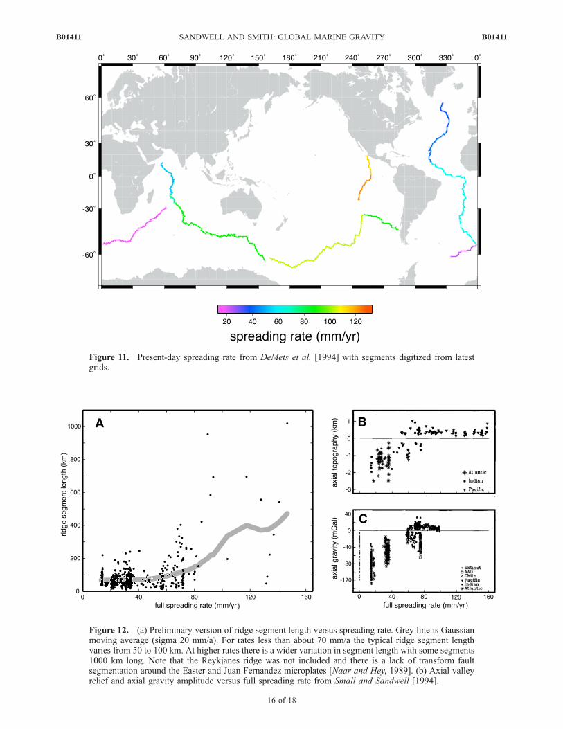
Figure 11. Present-day spreading rate from DeMets et al. [1994] with segments digitized from latestgrids.

Figure 12. (a) Preliminary version of ridge segment length versus spreading rate. Grey line is Gaussianmoving average (sigma 20 mm/a). For rates less than about 70 mm/a the typical ridge segment lengthvaries from 50 to 100 km. At higher rates there is a wider variation in segment length with some segments1000 km long. Note that the Reykjanes ridge was not included and there is a lack of transform faultsegmentation around the Easter and Juan Fernandez microplates [Naar and Hey, 1989]. (b) Axial valleyrelief and axial gravity amplitude versus full spreading rate from Small and Sandwell [1994].


16 of 18

B01411

[43] Acknowledgments. We thank the associate editor and reviewersfor suggesting improvements to the manuscript. This work was partlysupported by the National Science Foundation (OCE NAG5–13673) andthe Office of Naval Research (N00014-06-1-0140). The manuscript contentsare solely the opinions of the authors and do not constitute a statement ofpolicy, decision, or position on behalf of NOAA or the U. S. Government.

ReferencesAbbott, D. (1986), A statistical correlation between ridge crest offsets andspreading rate, J. Geophys. Res., 13, 157–160.

Amarouche, L., P. Thibaut, O. Z. Zanife, J.-P. Dumont, P. Vincent, andN. Steunou (2004), Improving the Jason-1 ground retracking to betteraccount for attitude effects, Mar. Geod., 27, 171–197, doi:10.1080/01490410490465210.

Andersen, O. B., and P. Knudsen (1998), Global marine gravity field fromthe ERS-1 and GEOSAT geodetic mission altimetry, J. Geophys. Res.,103, 8129–8137, doi:10.1029/97JC02198.

Baudry, N., and S. Calmant (1991), 3-D Modelling of seamount topographyfrom satellite altimetry, Geophys. Res. Lett., 18, 1143–1146, doi:10.1029/91GL01341.

Bendat, J. S., and A. G. Piersol (1986), Random Data Analysis and Mea-surement Procedures, 2nd ed., 566 pp., John Wiley, New York.

Bettadpur, S. V., and R. J. Eanes (1994), Geographical representation ofradial orbit perturbations due to ocean tides: Implications for satellitealtimetry, J. Geophys. Res., 99, 24,883–24,898, doi:10.1029/94JC02080.

Bird, P., Y. Y. Kagan, and D. D. Jackson (2002), Plate tectonics and earth-quake potential of spreading ridges and oceanic transform faults, in PlateBoundary Zones, Geodyn. Ser., vol. 30, edited by S. Stein and J. T.Freymueller, pp. 203–218, AGU, Washington, D.C.

Briggs, I. C. (1974), Machine contouring using minimum curvature, Geo-physics, 39, 39–48, doi:10.1190/1.1440410.

Brown, G. S. (1977), The average impulse response of a rough surface andits application, IEEE Trans. Antennas Propag., 25(1), 67 – 74,doi:10.1109/TAP.1977.1141536.

Brown, J., A. Colling, D. Park, J. Phillips, D. Rothery, and J.Wright (1998),The Ocean Basins: Their Structure and Evolution, 171 pp., Pergamon,Oxford, U. K.

Cande, S. C., J. M. Stock, R. D. Mueller, and T. Ishihara (2000), Cenozoicmotion between East and West Antarctica, Nature, 404, 145 –150,doi:10.1038/35004501.

Cazenave, A., P. Schaeffer, M. Berge, and C. Brossier (1996), High-resolu-tion mean sea surface computed with altimeter data of ERS-1(GeodeticMission) and TOPEX-POSEIDON, Geophys. J. Int., 125(3), 696–704,doi:10.1111/j.1365-246X.1996.tb06017.x.

Chelton, D. B., J. C. Reis, B. J. Haines, L. L. Fu, and P. S. Callahan (2001),Satellite altimetry, in Satellite Altimetry and Earth Sciences, edited byL. L. Fu and A. Cazenave, pp. 1–131, Academic, San Diego, Calif.

Cheney, R., J. Marsh, and B. Becklet (1983), Global mesoscale variabilityfrom collinear tracks of SEASAT altimeter data, J. Geophys. Res., 88,4343–4354, doi:10.1029/JC088iC07p04343.

Collette, B. (1974), Thermal contraction joints in spreading seafloor asorigin of fracture zones, Nature, 251, 299–300, doi:10.1038/251299a0.

DeMets, C., R. G. Gordon, D. F. Argus, and S. Stein (1994), Effect ofrecent revisions to the geomagnetic reversal timescale on estimates ofcurrent plate motions, Geophys. Res. Lett., 21, 2191–2194, doi:10.1029/94GL02118.

Dixon, T. H., M. Naraghi, M. K. McNutt, and S. M. Smith (1983), Bathy-metric prediction from Seasat altimeter data, J. Geophys. Res., 88, 1563–1571, doi:10.1029/JC088iC03p01563.

Fairhead, J. D., C. M. Green, and M. E. Odegard (2001), Satellite-derivedgravity having an impact on marine exploration, Leading Edge, 20, 873–876.

Fu, L.-L., and A. Cazenave (2001), Satellite Altimetry and Earth Sciences:A Handbook of Techniques and Applications, 463 pp., Academic, SanDiego, Calif.

Fu, L.-L., and D. B. Chelton (2001), Large-scale ocean circulation, inSatellite Altimetry and Earth Sciences, edited by A. Cazenave and L.-L.Fu, pp. 133–169, Academic, San Diego, Calif.

Gans, K. D., D. S. Wilson, and K. C. Macdonald (2003), Pacific plategravity lineaments: Extension or thermal contraction?, Geochem. Geo-phys. Geosyst., 4(9), 1074, doi:10.1029/2002GC000465.

Gille, S. T., M. M. Yale, and D. T. Sandwell (2000), Global correlationof mesoscale ocean variability with seafloor roughness from satellitealtimetry, Geophys. Res. Lett., 27(9), 1251 – 1254, doi:10.1029/1999GL007003.

Goff, J. A. (1991), A global and regional stochastic-analysis of near-ridgeabyssal hill morphology, J. Geophys. Res., 96(B13), 21,713–21,737,doi:10.1029/91JB02275.

Goff, J. A., W. H. F. Smith, and K. M. Marks (2004), The contributions ofabyssal hill morphology and noise to altimetric gravity fabric, Oceano-graphy, 17(1), 24–37.

Gregg, P. C., J. Lin, M. D. Behn, and L. G. J. Montesi (2007), Spreadingrate dependence of gravity anomalies along oceanic transform faults,Nature, 448, 183–187, doi:10.1038/nature05962.

Haxby, W. F., and J. K. Weissel (1986), Evidence for small-scale mantleconvection from Seasat altimeter data, J. Geophys. Res., 91(B3), 3507–3520, doi:10.1029/JB091iB03p03507.

Haxby, W. F., G. D. Karner, J. L. LaBrecque, and J. K. Weissel (1983),Digital images of combined oceanic and continental data sets and theiruse in tectonic studies, Eos Trans. AGU, 64(52), 995–1004.

Hieronymus, C. F. (2004), Control on seafloor spreading geometries bystress- and strain-induced lithospheric weakening, Earth Planet. Sci.Lett., 222, 177–189, doi:10.1016/j.epsl.2004.02.022.

Hwang, C., and B. Parsons (1996), An optimal procedure for derivingmarine gravity from multi-satellite altimetry, J. Geophys. Int., 125,705–719, doi:10.1111/j.1365-246X.1996.tb06018.x.

Imel, D. A. (1994), Evaluation of the TOPEX/POSEIDON dual-frequencyionospheric correction, J. Geophys. Res., 99, 24,895 – 24,906,doi:10.1029/94JC01869.

Jayne, S. R., L. C. St. Laurent, and S. T. Gille (2004), Connections betweenocean bottom topography and the Earth’s Climate, Oceanography, 17(1),65–74.

Jung, W. Y., and P. R. Vogt (1992), Predicting bathymetry from Geosat-ERM and shipborne profiles in the South Atlantic ocean, Tectonophysics,210, 235–253, doi:10.1016/0040-1951(92)90324-Y.

Kastens, K. K. (1987), A compendium of causes and effects of processes attransform faults and fracture zones, Rev. Geophys., 25(7), 1554–1562,doi:10.1029/RG025i007p01554.

Klees, R., R. Koop, P. Visser, and J. van den IJssel (2000), Efficient gravityfield recovery from GOCE gravity gradient observations, J. Geod., 74(7–8), 561–571, doi:10.1007/s001900000118.

Korenaga, J. (2007), Thermal cracking and deep hydration of oceanic litho-sphere: A key to generation of plate tectonics?, J. Geophys. Res., 112,B05408, doi:10.1029/2006JB004502.

Kumar, R. R., and R. G. Gordon (2009), Horizontal thermal contraction ofoceanic lithosphere: The ultimate limit to the rigid plate approximation,J. Geophys. Res., 114, B01403, doi:10.1029/2007JB005473.

Kunze, E., and S. G. Llewellyn Smith (2004), The role of small-scaletopography in turbulent mixing of the global ocean, Oceanography,17(1), 55–64.

Lachenbruch, A. H. (1973), A simple mechanical model for oceanic spreadingcenters, J. Geophys. Res., 78, 3395–3417, doi:10.1029/JB078i017p03395.

Lawver, L. A., L. M. Gahagan, and M. F. Coffin (1992), The developmentof paleoseaways around Antarctica, in The Antarctic Paleoenvironment:A Perspective on Global Change, Geophys. Monogr. Ser., vol. 56, editedby J. P. Kennett and D. A. Warnke, pp. 7–30, AGU, Washington, D. C.

Laxon, S., and D. McAdoo (1994), Arctic Ocean gravity field derived fromERS-1 satellite altimetry, Science, 265(5172), 621–624, doi:10.1126/science.265.5172.621.

Lemoine, F. G., et al. (1998), The development of the joint NASA CSFCand the national Imagery and Mapping Agency (NIMA) geopotentialmodel EGM96, 320 pp., NASA Goddard Space Flight Cent., Greenbelt,Md.

Le-Traon, P.-Y., and R. Morrow (2001), Ocean currents and eddies, inSatellite Altimetry and Earth Sciences, edited by A. Cazenave and L.-L.Fu, pp. 175–215, Academic, San Diego, Calif.

Lillibridge, J., and R. Cheney (1997), The Geosat Altimeter JGM-3 GDRs[CD-ROM], NOAA, Silver Spring, Md.

Lillibridge, J. L., W. H. F. Smith, R. Scharrroo, and D. T. Sandwell (2004),The Geosat geodetic mission 20th anniversary data product, Eos Trans.AGU, 85(47), Fall Meet. Suppl., Abstract SF43A–0786.

Lin, J., and J. Phipps Morgan (1992), The spreading rate dependence ofthree-dimensional mid-ocean ridge gravity structure, Geophys. Res. Lett.,19, 13–16, doi:10.1029/91GL03041.

Macdonald, K. C., P. J. Fox, L. J. Perram, M. F. Eisen, R. M. Haymon, S. P.Miller, S. M. Carbotte, M. H. Cormier, and A. N. Shor (1988), A newview of the mid-ocean ridge from the behavior of ridge-axis discontinu-ities, Nature, 335(6187), 217–225, doi:10.1038/335217a0.

Magde, L. S., and D. W. Sparks (1997), Three-dimensional mantle upwel-ling, melt generation, and melt migration beneath segment slow spread-ing ridge, J. Geophys. Res., 102, 20,571 – 20,583, doi:10.1029/97JB01278.

Maia, M. (2006), Comparing the use of marine and satellite data for geo-dynamic studies, paper presented at 15 Years of Progress in Radar Alti-metry Symposium, Eur. Space Agency, Venice, Italy.

Marks, K. M., and W. H. F. Smith (2007), Some remarks on resolving sea-mounts in satellite gravity, Geophys. Res. Lett., 34, L03307, doi:10.1029/2006GL028857.


17 of 18

B01411

Maus, S., C. M. Green, and J. D. Fairhead (1998), Improved ocean-geoidresolution from retracked ERS-1 satellite altimeter waveforms, Geophys.J. Int., 134(1), 243–253, doi:10.1046/j.1365-246x.1998.00552.x.

McAdoo, D., and S. Laxon (1997), Antarctic tectonics: Constraints from anERS-1 satellite marine gravity field, Science, 276(5312), 556–561,doi:10.1126/science.276.5312.556.

Menard, H. W. (1967), Sea floor spreading topography and second layer,Science, 157(3791), 923–924, doi:10.1126/science.157.3791.923.

Menke, W. (1991), Applications of the POCS inversion method to inter-polating topography and other geophysical fields, Geophys. Res. Lett.,18(3), 435–438, doi:10.1029/90GL00343.

Monaldo, F. (1988), Expected differences between buoy and radar altimeterestimates of wind speed and significant wave height and their implica-tions on buoy-altimeter comparisons, J. Geophys. Res., 93(C3), 2285–2302, doi:10.1029/JC093iC03p02285.

Mueller, R. D., W. R. Roest, J.-Y. Royer, L. M. Gahagan, and J. G. Sclater(1997), Digital isochrons of the world’s ocean floor, J. Geophys. Res.,102, 3211–3214, doi:10.1029/96JB01781.

Munk, W., and C. Wunch (1998), Abyssal recipes II: Energetics of todayand wind mixing, Deep Sea Res., Part I, 45, 1977–2010, doi:10.1016/S0967-0637(98)00070-3.

Naar, D. F., and R. N. Hey (1989), Speed limit for oceanic transform faults,Geology, 17(5), 420 – 422, doi:10.1130/0091-7613(1989)017<0420:SLFOTF>2.3.CO;2.

Oldenburg, D. W., and J. N. Brune (1975), An explanation for the ortho-gonality of ocean ridges and transform faults, J. Geophys. Res., 80(17),2575–2585, doi:10.1029/JB080i017p02575.

Parmentier, E. M., and J. Phipps Morgan (1990), Spreading rate dependenceof three-dimensional structure in oceanic spreading centres, Nature, 348,325–328, doi:10.1038/348325a0.

Pavlis, N. K., S. A. Holmes, S. C. Kenyon, and J. K. Factor (2007), Earthgravitational model to degree 2160: Status and progress, paper presentedat XXIV General Assembly, pp. 2–13, Int. Union of Geod. and Geo-phys., Perugia, Italy.

Pavlis, N. K., S. A. Holmes, S. C. Kenyon, and J. K. Factor (2008), AnEarth gravitational model to degree 2160, paper presented at GeneralAssembly, Eur. Geosci. Union, Vienna.

Picaut, J., and A. J. Busalacchi (2001), Tropical ocean variability, in Sa-tellite Altimetry and Earth Sciences, edited by A. Cazenave and L.-L. Fu,pp. 217–236, Academic, San Diego, Calif.

Ponte, R. M. (1994), Understanding the relation between wind- and pres-sure-driven sea level variability, J. Geophys. Res., 99, 8033–8039,doi:10.1029/94JC00217.

Ramillien, G., and A. Cazenave (1997), Global bathymetry derived fromaltimeter data of the ERS-1 Geodetic Mission, J. Geodyn., 23(2), 129–149, doi:10.1016/S0264-3707(96)00026-9.

Raney, R. K., W. H. F. Smith, D. T. Sandwell, J. R. Jensen, D. L. Porter, andE. Reynolds (2003), Abyss-Lite: Improved bathymetry from a dedicatedsmall satellite delay-Doppler radar altimeter, paper presented at Interna-tional Geoscience and Remote Sensing Symposium IGARSS2003, IEEE,Toulouse, France.

Reigber, C., et al. (2002), A high quality global gravity field model fromCHAMP GPS tracking data and accelerometer (EIGEN-1S), Geophys.Res. Lett., 29(14), 1692, doi:10.1029/2002GL015064.

Rummel, R., and R. H. N. Haagmans (1990), Gravity gradients fromsatellite altimetry, Mar. Geod., 14, 1–12.

Sandwell, D. T. (1984), A detailed view of the South Pacific from satellitealtimetry, J. Geophys. Res., 89, 1089–1104, doi:10.1029/JB089iB02p01089.

Sandwell, D. T. (1986), Thermal stress and the spacings of transform faults,J. Geophys. Res., 91, 6405–6417, doi:10.1029/JB091iB06p06405.

Sandwell, D. T. (1987), Biharmonic spline interpolation of Geos-3 andSeasat altimeter data, Geophys. Res. Lett., 14(2), 139–142, doi:10.1029/GL014i002p00139.

Sandwell, D., and Y. Fialko (2004), Warping and cracking of the Pacificplate by thermal contraction, J. Geophys. Res., 109, B10411,doi:10.1029/2004JB003091.

Sandwell, D. T., and W. H. F. Smith (1997), Marine gravity anomaly fromGeosat and ERS-1 satellite altimetry, J. Geophys. Res., 102, 10,039–10,054, doi:10.1029/96JB03223.

Sandwell, D. T., and W. H. F. Smith (2005), Retracking ERS-1 altimeterwaveforms for optimal gravity field recovery, Geophys. J. Int., 163, 79–89, doi:10.1111/j.1365-246X.2005.02724.x.

Sandwell, D. T., and B. Zhang (1989), Global mesoscale variability fromthe Geosat exact repeat mission: Correlation with ocean depth, J. Geo-phys. Res., 94, 17,971–17,984, doi:10.1029/JC094iC12p17971.

Schouten, H., K. D. Klitgord, and J. A. Whitehead (1985), Segmentation ofmid-ocean ridges, Nature, 317, 225–229, doi:10.1038/317225a0.

Shum, C. K., et al. (2001), Recent advances in ocean tidal science, J. Geod.Soc. Jpn., 47(1), 528–537.

Shum, C. K., P. A. M. Abusali, H. Lee, J. Ogle, R. K. Raney, J. C. Reis,W. H. F. Smith, D. Svehla, and C. Zhao (2009), Science requirements forABYSS: A proposed Space Station RADAR altimeter to map globalbathymetry, IEEE Trans. Geosci. Remote Sens., in press.

Small, C. (1994), A global analysis of mid-ocean ridge axial topography,Geophys. J. Int., 116, 64–84, doi:10.1111/j.1365-246X.1994.tb02128.x.

Small, C., and D. T. Sandwell (1992), An analysis of ridge axis gravityroughness and spreading rate, J. Geophys. Res., 97(B3), 3235–3245,doi:10.1029/91JB02465.

Small, C., and D. T. Sandwell (1994), Imaging mid-ocean ridge transitionswith satellite gravity, Geology, 22, 123–126.

Smith, W. H. F. (1998), Seafloor tectonic fabric from satellite altimetry,Annu. Rev. Earth Planet. Sci., 26(1), 697–747, doi:10.1146/annurev.earth.26.1.697.

Smith, W. H. F., and D. T. Sandwell (1994), Bathymetric prediction frondense satellite altimetry and sparse shipboard bathymetry, J. Geophys.Res., 99, 21,803–21,824, doi:10.1029/94JB00988.

Smith, W. H. F., and D. T. Sandwell (1997), Global sea floor topographyfrom satellite altimetry and ship depth soundings, Science, 277(5334),1956–1962, doi:10.1126/science.277.5334.1956.

Smith, W. H. F., and P. Wessel (1990), Gridding with continuous curvaturesplines in tension, Geophysics, 55(3), 293–305, doi:10.1190/1.1442837.

Tapley, B. D., and M. C. Kim (2001), Applications to geodesy, in SatelliteAltimetry and Earth Sciences, edited by A. Cazenave and L.-L. Fu,pp. 371–403, Academic, San Diego, Calif.

Tapley, B., et al. (2005), GGM02 - An improved Earth gravity model fromGRACE, J. Geod., 79, 467–478, doi:10.1007/s00190-005-0480-z.

Turcotte, D. L. (1974), Are transform faults thermal contraction cracks?,J. Geophys. Res., 79, 2573–2577, doi:10.1029/JB079i017p02573.

Wessel, P., and D. Bercovici (1998), Interpolation with splines in tension: AGreen’s function approach, Math. Geol., 30(1), 77–93, doi:10.1023/A:1021713421882.

Wessel, P., and A. B. Watts (1988), On the accuracy of marine gravitymeasurements, J. Geophys. Res., 93(B1), 393 – 413, doi:10.1029/JB093iB01p00393.

Yale, M. M. (1997), Modeling upper mantle rheology with numerical ex-periments and mapping marine gravity with satellite altimetry, Ph.D.thesis, 118 pp., Univ. of Calif., San Diego, La Jolla.

��D. T. Sandwell, Scripps Institution of Oceanography, University of

California, San Diego, La Jolla, CA 92093-0225, USA. ([email protected])W. H. F. Smith, Laboratory for Satellite Altimetry, NOAA, 1335 East-

West Highway, Room 5408, Silver Spring, MD 20910, USA.


18 of 18

B01411

global marine gravity from retracked geosat and ers-1 altimetry

Documents