global lidar remote sensing of stratospheric aerosols and

Global LIDAR Remote Sensing of Stratospheric Aerosols and

Comparison with WACCM/CARMA

CESM Whole Atmosphere Working Group Meeting 16 - 17 February 2011National Center for Atmospheric Research – Boulder, Colorado

Acknowledge: Dr. Michael Mills and Jason English for basis of current working model.

Ryan R. Neely IIIAdvisors: Susan Solomon, Brian Toon, Jeff Thayer and Michael Hardesty

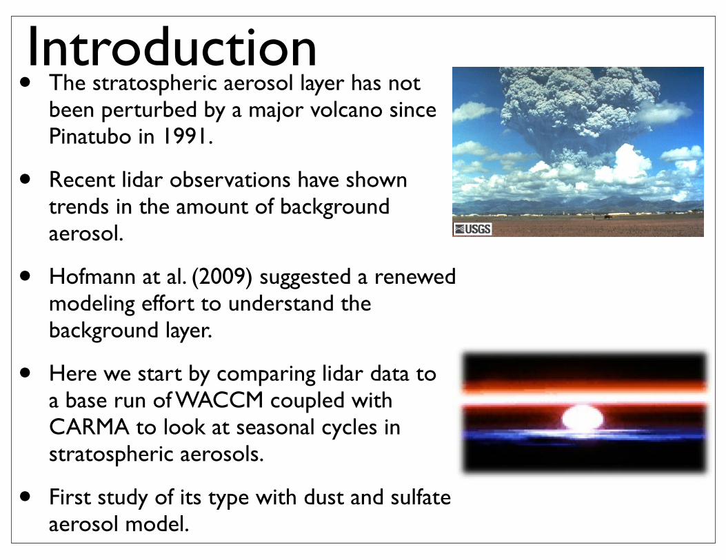
Introduction• The stratospheric aerosol layer has not

been perturbed by a major volcano since Pinatubo in 1991.

• Recent lidar observations have shown trends in the amount of background aerosol.

• Hofmann at al. (2009) suggested a renewed modeling effort to understand the background layer.

• Here we start by comparing lidar data to a base run of WACCM coupled with CARMA to look at seasonal cycles in stratospheric aerosols.

• First study of its type with dust and sulfate aerosol model.

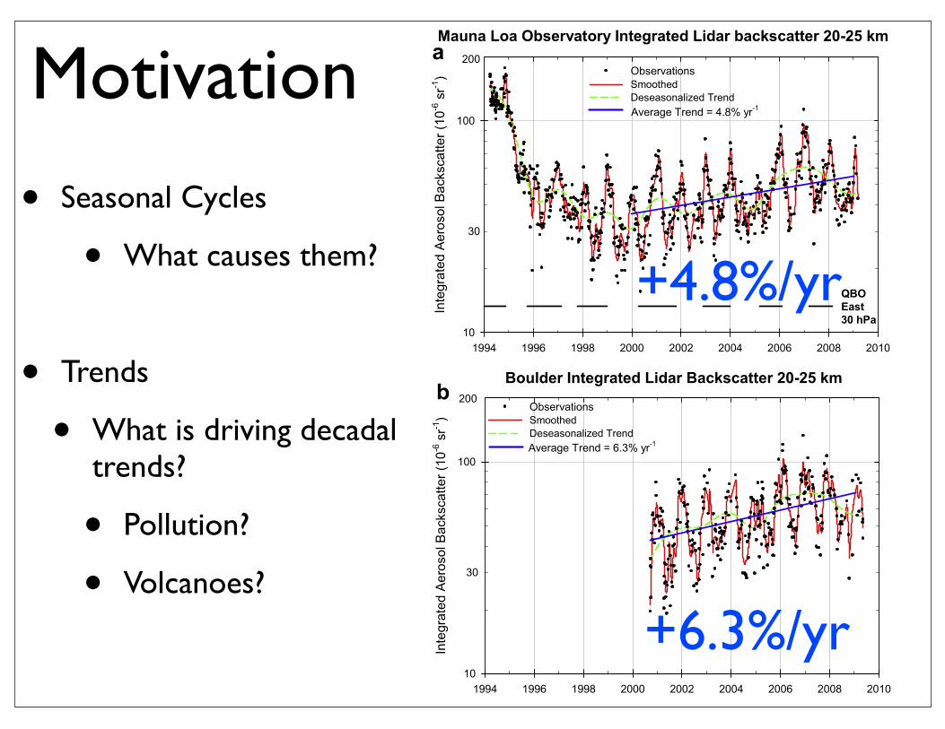
Motivation

• Seasonal Cycles

• What causes them?

• Trends

• What is driving decadal trends?

• Pollution?

• Volcanoes?

eruption observed at Boulder. Three soundings shortly aftereach of these events were not included in the trend data.Figure 2a shows the Mauna Loa Observatory Nd:YAG lidar20–25 km integrated backscatter data from 1994, when thelidar began operating, to early 2009. The data have beenanalyzed using the technique of Thoning et al. [1989] tosmooth the data, remove the seasonal variation, and deter-mine the trend curve and growth rate (determined by differ-entiating the deseasonalized trend curves). There is a biennialcomponent in the deseasonalized trend in Figure 2a, likelyrelated to the quasi-biennial oscillation (QBO) in tropicalwinds, as will be discussed later. From 1994 to 1996 thedecay of aerosol from the 1991 Pinatubo eruption dominatesthe data [Barnes and Hofmann, 1997]. From 1996 to 2000there was a slightly decreasing trend at Mauna Loa,possibly due to remnants of the Pinatubo eruption. How-ever, after 2000 there is a decidedly increasing aerosolbackscatter trend. The magnitude of the aerosol backscattertrend at Mauna Loa Observatory varies with altitude. Themaximum trend occurs in the 20–25 km region with anaverage value of 4.8% per year, and about 3.3% per yearfor the total column for the 2000–2009 period (thestandard error in determining these trends is about ±5%of the trend value). Figure 2b, for the 20–25 km range atBoulder, indicates an increasing average trend of 6.3% peryear for the 2000–2009 period.[7] It is important to note that the seasonal increase in

aerosol backscatter (summer to winter) is about 2.5 timeslarger than the backscatter magnitude of the 2000–2009trend. Therefore, the trend would be difficult to detect byany method that cannot resolve the seasonal variation. Weare not aware of other surface-based or satellite lidar orsatellite limb extinction instruments that have reportedobserving the background aerosol seasonal variation or along-term trend. Finally, since 1996, the peak-to-peak mag-nitude of the detrended, smoothed annual cycle at Mauna

Figure 1. Seasonal average aerosol backscatter ratio profiles at (a) Mauna Loa Observatory and (b) Boulder, Colorado.The backscatter ratio is defined as the ratio of the total backscatter (aerosol plus molecular backscatter) to the molecularbackscatter. A ratio of 1.0 indicates pure atmospheric molecular scattering. The inset in Figure 1a shows the seasonal cycleamplitude versus time.

Figure 2. Integrated backscatter for the 20–25 km altituderange at (a) Mauna Loa Observatory and (b) Boulder,Colorado.

L15808 HOFMANN ET AL.: INCREASE IN STRATOSPHERIC AEROSOL L15808

2 of 5

+4.8%/yr

+6.3%/yr

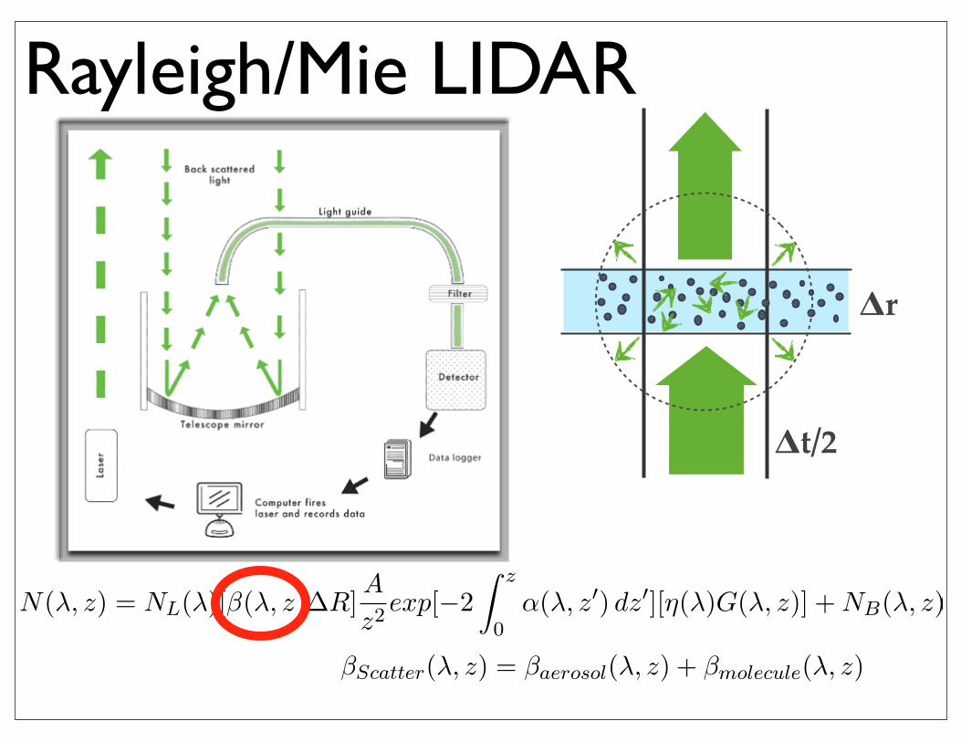
Rayleigh/Mie LIDAR

Δt/2

Δr

1.3 Lidar Remote Sensing of Stratospheric Aerosols Chapter 1: Introduction

Figure 1.7: Depiction of typical raw lidar data collected in Boulder, CO. Two

profiles are collected with this instrument in order to create a single profile from

2km to 35km. Separate upper and lower profiles are needed due to the large

dynamic range needed to examine the entire altitude range. The exponential

nature of the atmosphere is clearly evident in both profiles. Adapted from

http : //www.mlo.noaa.gov/programs/gmdlidar/mlo/gmdlidar mlo.html.

N(λ, z) = NL(λ)[β(λ, z)∆R]A

z2exp[−2

� z

0α(λ, z�) dz�][η(λ)G(λ, z)] +NB(λ, z)(1.1)

The backscatter and extinction coefficients may be separated into molecular and

aerosol components as seen in equations (2) and (3). The extinction coefficient

has an additional term which accounts for extinction due to absorption by

different trace molecules in the atmosphere.

βScatter(λ, z) = βaerosol(λ, z) + βmolecule(λ, z) (1.2)

18

1.3 Lidar Remote Sensing of Stratospheric Aerosols Chapter 1: Introduction

Figure 1.7: Depiction of typical raw lidar data collected in Boulder, CO. Two

profiles are collected with this instrument in order to create a single profile from

2km to 35km. Separate upper and lower profiles are needed due to the large

dynamic range needed to examine the entire altitude range. The exponential

nature of the atmosphere is clearly evident in both profiles. Adapted from

http : //www.mlo.noaa.gov/programs/gmdlidar/mlo/gmdlidar mlo.html.

N(λ, z) = NL(λ)[β(λ, z)∆R]A

z2exp[−2

� z

0α(λ, z�) dz�][η(λ)G(λ, z)] +NB(λ, z)(1.1)

The backscatter and extinction coefficients may be separated into molecular and

aerosol components as seen in equations (2) and (3). The extinction coefficient

has an additional term which accounts for extinction due to absorption by

different trace molecules in the atmosphere.

βScatter(λ, z) = βaerosol(λ, z) + βmolecule(λ, z) (1.2)

18

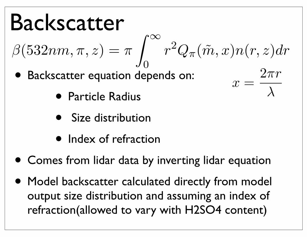
Backscatter

• Backscatter equation depends on:

• Particle Radius

• Size distribution

• Index of refraction

• Comes from lidar data by inverting lidar equation

• Model backscatter calculated directly from model output size distribution and assuming an index of refraction(allowed to vary with H2SO4 content)

2.3 WACCM Data Analysis Chapter 2: Data Analysis

that were adapted for use in MATLAB by Matzler (2002). Within these calcu-

lations, the particles were assumed to be spherical and, for particles with dust

core, the particle does not behave like a coated sphere. This essentially means

that the total radius of a particle with a dust core is large enough that the light

will not interact with dust core. The complex component index of refraction

was also assumed to be zero because of the lack of data for these particles at

this wavelength. This causes the aerosols in the model to have zero absorption

which may cause an over estimate of their true backscatter. The real compo-

nent was allowed to vary as a function of the mass percent of H2SO4 present

within the aerosol. Data for this dependence is found in the work of Palmer

(1975). A fit was applied to the data so that a continuous function for the index

of refraction as function of the mass percent of H2SO4 could be made and used

to determine the index of refraction for the complete range of values for the

aerosols within the model. The index of refraction of the aerosol should also

be a function of temperature and pressure but for the wavelength of 532nm the

variation is small compared to that caused by the variation in H2SO4 content

(Redemann et al., 2000; Massie, 1994; Myhre et al., 2003; Muller et al., 1999;

Zhao et al., 1997).

To convert the model output into backscatter coefficients at the wavelength

of the lidar, the integral for calculating the backscatter over a continuous size

distribution of particles (2.8) was converted into a Riemann sum to account for

the discrete number of radius bins used in the model (2.9). This calculation

was done for each type of aerosol element separately and combined later.

β(532nm,π, z) = π

� ∞

0r2Qπ(m, x)n(r, z)dr (2.9)

β(532nm,π, z) = π36�

rBin=1

r2BinQπ(m, x)n(rBin, z)(rBin − rBin−1) (2.10)

38

2.3 WACCM Data Analysis Chapter 2: Data Analysis

The size distribution n(rBin, z) is calculated using the mass distribution of

the bins and the total aerosol number density calculated by the model:

n(rBin, z) =BinMass(r)

36�r=1

BinMass(r)

× TotalNumberNumberDensity (2.11)

In both equations x is the size parameter defined as

x =2πr

λ(2.12)

and m is the complex index of refraction used in the Mie calculation of

the backscatter efficiency Qπ. Qπ is a special case of the extinction efficiency,

Qext, for a scattering angle equal to π and may be defined using only the size

parameter and a series of the a and b Mie coefficients (Matzler, 2002; Bohren

and Huffman, 1983).

Qext =2

x2

∞�

n=1

(2n+ 1)Re(an + bn) (2.13)

Qπ =1

x2

��

∞�

n=1

(2n+ 1)(−1)n(an − bn)

��

2

(2.14)

Here n = ∞ is approximated with nmax = x+4x1/3+2 as suggested by Bohren

and Huffman (1983).

To aid the speed of these calculations, a look up table of scattering efficiency

terms, Qext and Qπ, was compiled as a function of sulfate particle size param-

eter and index of refraction for the range of values represented in the model

output data. The sulfate look up table has Q values corresponding to 10000 ra-

dius size parameters and 107 indices of refraction corresponding to the percent

weight of sulfuric acid in the particle. For the actual scattering calculation of

the sulfate aerosols the closest scattering efficiency term above and below the

actual size parameter and above and below the actual mass percent of H2SO4

39

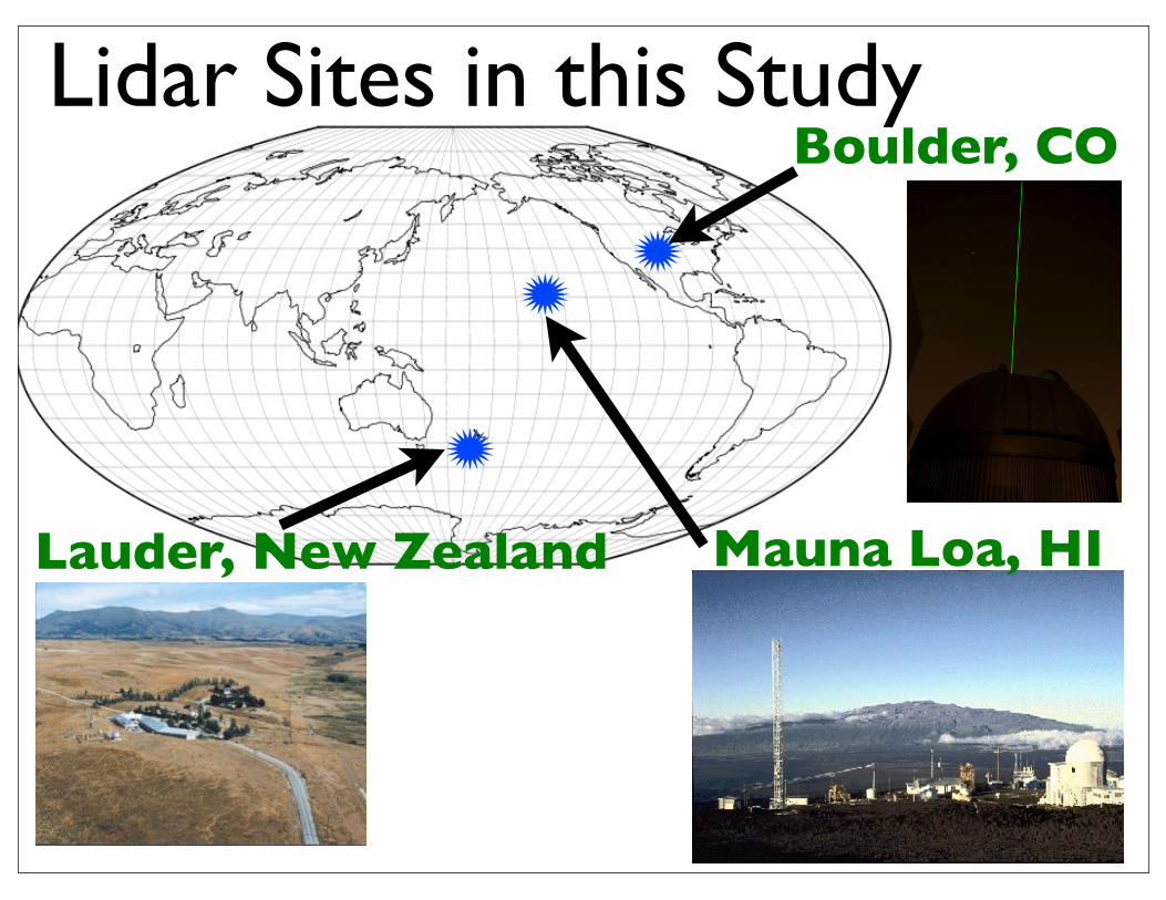
Lidar Sites in this Study

Lauder, New Zealand

Boulder, CO

Mauna Loa, HI

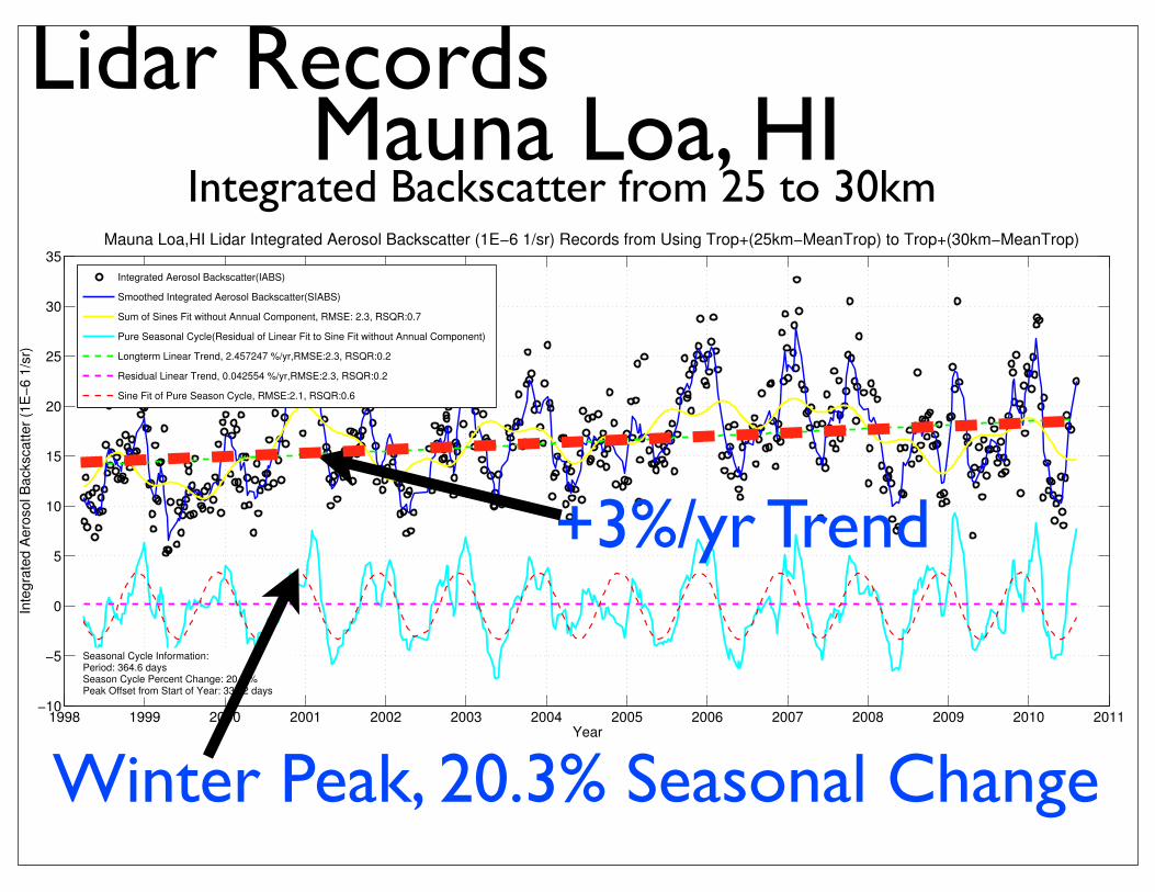
Lidar Records

1998 1999 2000 2001 2002 2003 2004 2005 2006 2007 2008 2009 2010 2011−10

−5

0

5

10

15

20

25

30

35

Inte

gra

ted

Ae

roso

l Ba

cksc

att

er

(1E−

6 1

/sr)

Year

Mauna Loa,HI Lidar Integrated Aerosol Backscatter (1E−6 1/sr) Records from Using Trop+(25km−MeanTrop) to Trop+(30km−MeanTrop)

Integrated Aerosol Backscatter(IABS)

Smoothed Integrated Aerosol Backscatter(SIABS)

Sum of Sines Fit without Annual Component, RMSE: 2.3, RSQR:0.7

Pure Seasonal Cycle(Residual of Linear Fit to Sine Fit without Annual Component)

Longterm Linear Trend, 2.457247 %/yr,RMSE:2.3, RSQR:0.2

Residual Linear Trend, 0.042554 %/yr,RMSE:2.3, RSQR:0.2

Sine Fit of Pure Season Cycle, RMSE:2.1, RSQR:0.6

Seasonal Cycle Information:Period: 364.6 daysSeason Cycle Percent Change: 20.3 %Peak Offset from Start of Year: 333.2 days

Mauna Loa, HI

Winter Peak, 20.3% Seasonal Change

+3%/yr Trend

Integrated Backscatter from 25 to 30km

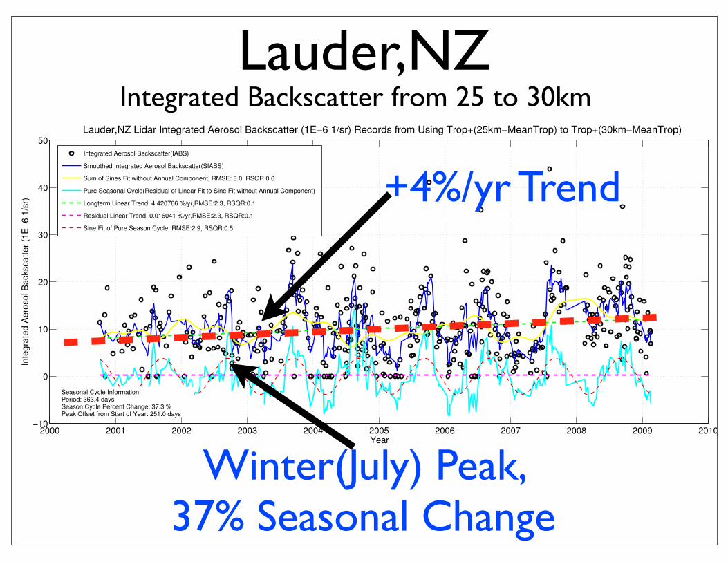
Lauder,NZ

2000 2001 2002 2003 2004 2005 2006 2007 2008 2009 2010−10

0

10

20

30

40

50

Inte

gra

ted

Ae

roso

l Ba

cksc

att

er

(1E

−6

1/s

r)

Year

Lauder,NZ Lidar Integrated Aerosol Backscatter (1E−6 1/sr) Records from Using Trop+(25km−MeanTrop) to Trop+(30km−MeanTrop)









Winter(July) Peak, 37% Seasonal Change

+4%/yr Trend


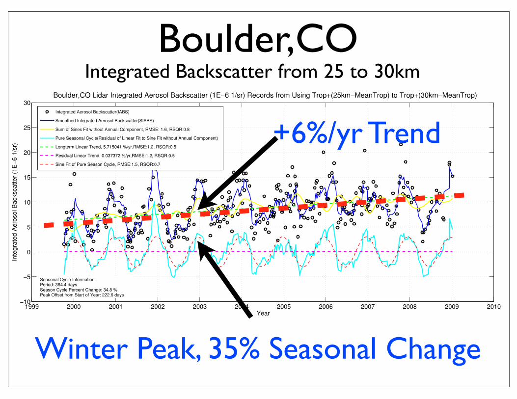
Boulder,CO

1999 2000 2001 2002 2003 2004 2005 2006 2007 2008 2009 2010−10

−5

0

5

10

15

20

25

30

Inte

gra

ted

Ae

roso

l Ba

cksc

att

er

(1E−

6 1

/sr)

Year

Boulder,CO Lidar Integrated Aerosol Backscatter (1E−6 1/sr) Records from Using Trop+(25km−MeanTrop) to Trop+(30km−MeanTrop)









Winter Peak, 35% Seasonal Change

+6%/yr Trend


WACCM Setup• WACCM version 3.1.9

• 4x5 degree resolution

• 66 vertical levels

• Model top near 140 km

• Vertical spacing of 1-1.75km in the stratosphere

• 25 year run, averaging last 10 years

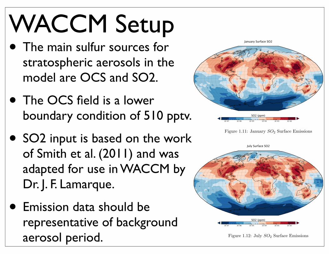
WACCM Setup• The main sulfur sources for

stratospheric aerosols in the model are OCS and SO2.

• The OCS field is a lower boundary condition of 510 pptv.

• SO2 input is based on the work of Smith et al. (2011) and was adapted for use in WACCM by Dr. J. F. Lamarque.

• Emission data should be representative of background aerosol period.

1.4 WACCM and CARMA Chapter 1: Introduction

represents chemical and physical processes in the middle atmosphere. Within

this mechanism are the species for the Ox, NOx, HOx, ClOx, and BrOx chemical

families, as well as CH4 and its products, SO2, SO3, SO,H2SO4, CS2 and OCS.

Figure 1.11: January SO2 Surface Emissions

Figure 1.12: July SO2 Surface Emissions

The main sulfur sources for stratospheric aerosols in the model are OCS

and SO2. The OCS field is a lower boundary condition everywhere of 510 pptv.

The SO2 emissions are handled in a subroutine of MOZART within WACCM.

24

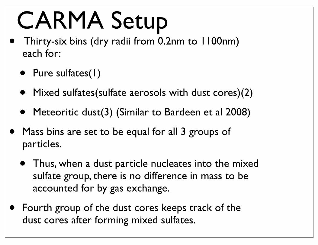
CARMA Setup• Thirty-six bins (dry radii from 0.2nm to 1100nm)

each for:

• Pure sulfates(1)

• Mixed sulfates(sulfate aerosols with dust cores)(2)

• Meteoritic dust(3) (Similar to Bardeen et al 2008)

• Mass bins are set to be equal for all 3 groups of particles.

• Thus, when a dust particle nucleates into the mixed sulfate group, there is no difference in mass to be accounted for by gas exchange.

• Fourth group of the dust cores keeps track of the dust cores after forming mixed sulfates.

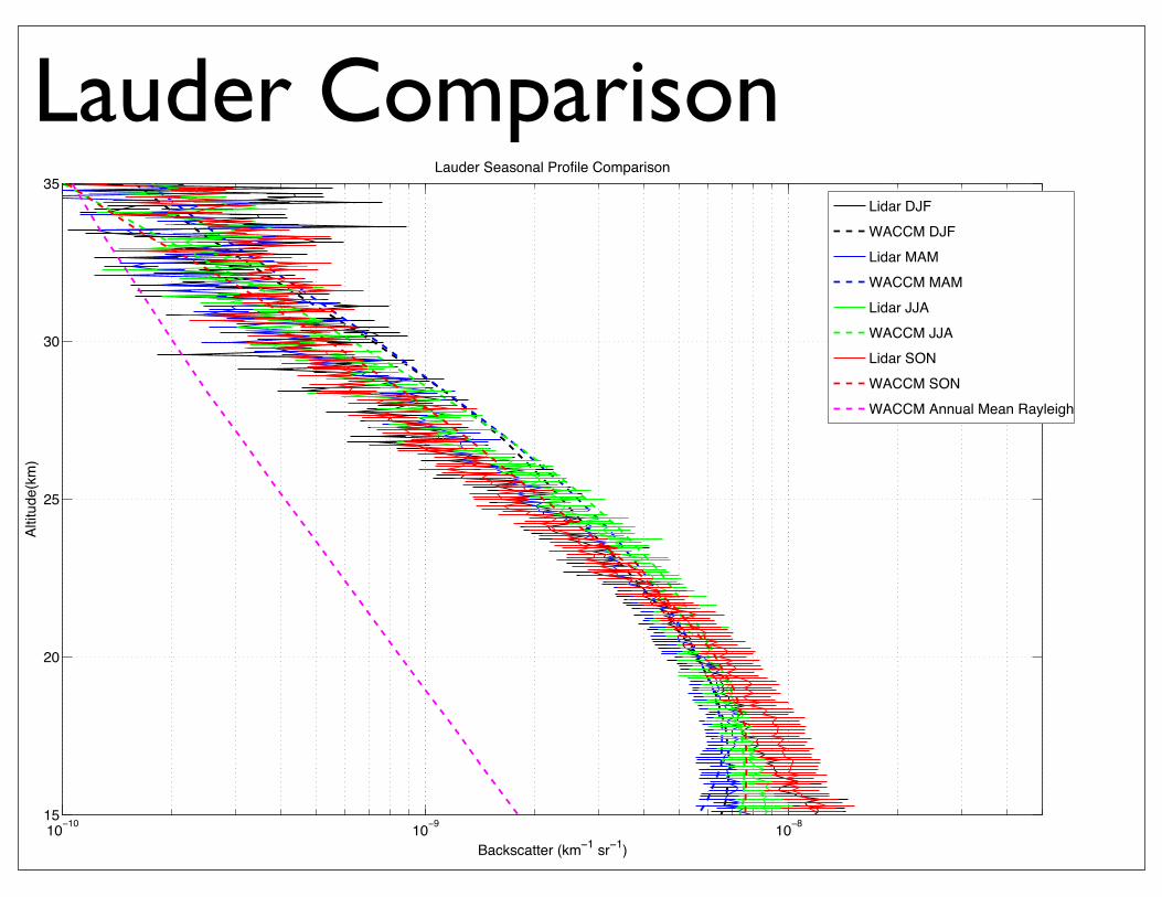
Lauder Comparison

10 10 10 9 10 815

20

25

30

35Lauder Seasonal Profile Comparison

Backscatter (km 1 sr 1)

Altit

ude(

km)

Lidar DJFWACCM DJFLidar MAMWACCM MAMLidar JJAWACCM JJALidar SONWACCM SONWACCM Annual Mean Rayleigh

Mauna Loa Comparison

10 10 10 9 10 815

20

25

30

35Mauna Loa Seasonal Profile Comparison


Altit

ude(

km)


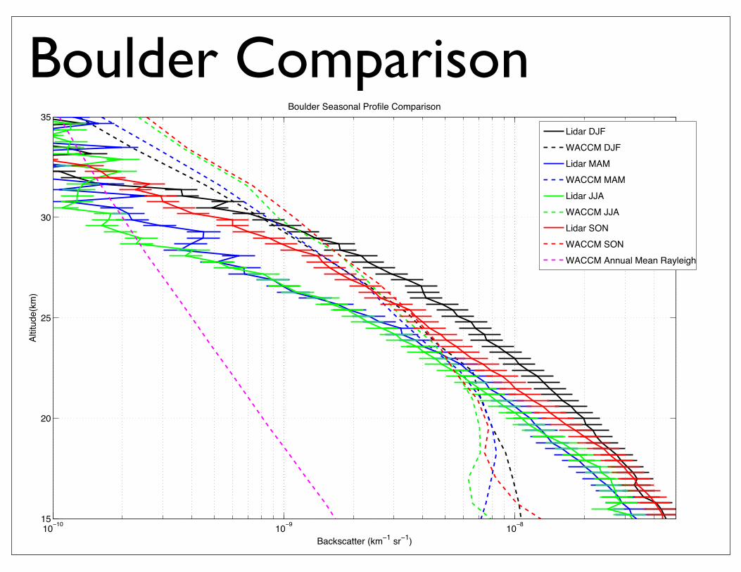
Boulder Comparison

10 10 10 9 10 815

20

25

30

35Boulder Seasonal Profile Comparison


Altit

ude(

km)


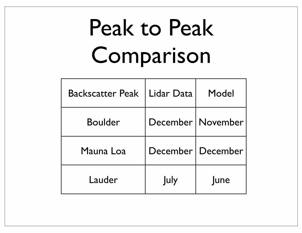
Peak to Peak Comparison

Backscatter Peak Lidar Data Model

Boulder December November

Mauna Loa December December

Lauder July June

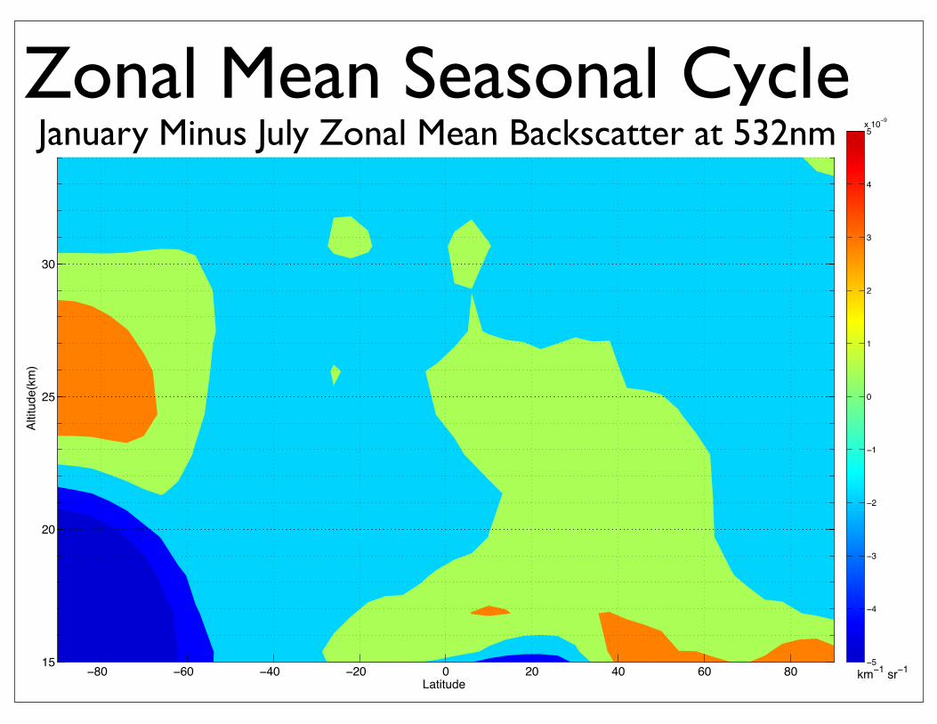
Zonal Mean Seasonal Cycle

Latitude

Altit

ude(

km)

WACCM Dust Sulfur January minus July Zonal Mean Backscatter at 532nm

80 60 40 20 0 20 40 60 8015

20

25

30

35

km 1 sr 15

4

3

2

1

0

1

2

3

4

5x 10 9

January Minus July Zonal Mean Backscatter at 532nm

1

1

1

2

2

2

3

3

3

4

4

4

5

5

5

6

6

6

7

7

7

8

8

8

9

9

9

10

10

10

11

11

11

12

12

12

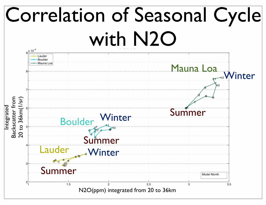
N 2O(ppm)

Inte

grat

ed B

acks

catte

r( sr

1 )

WACCM Dust Sulfur Monthly Integrated Backscatter Versus N 2O from 20km to 36km

1 1.5 2 2.5 3 3.52

3

4

5

6

7

8

9 x 10 8

LauderBoulderMauna Loa

Model Month

N2O(ppm) integrated from 20 to 36km

Inte

grat

ed

Back

scat

ter

from

20

to

36km

(1/s

r)

Boulder

Lauder

Mauna Loa

Winter

Text

Correlation of Seasonal Cycle with N2O

Summer

Winter

Summer

Winter

Summer

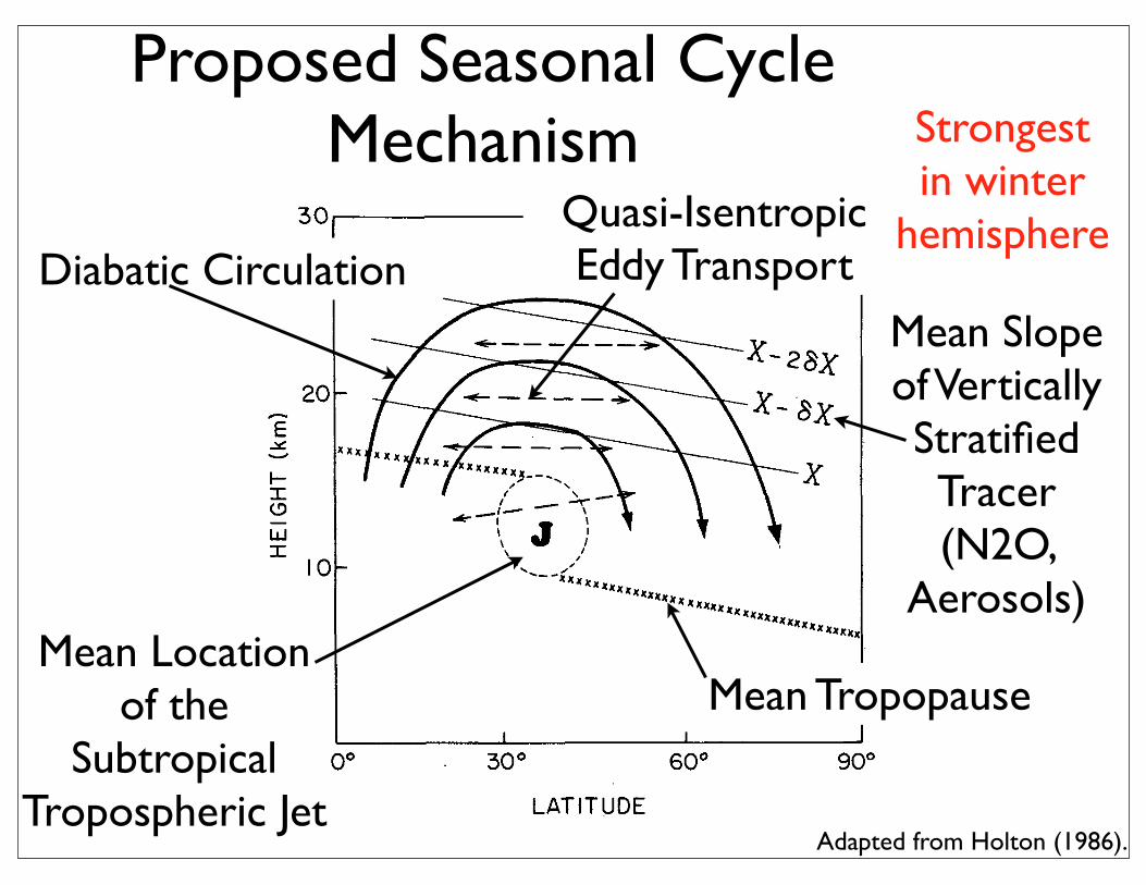
Proposed Seasonal Cycle Mechanism

Adapted from Holton (1986).

Diabatic CirculationQuasi-Isentropic Eddy Transport

Mean TropopauseMean Location

of the Subtropical

Tropospheric Jet

Mean Slope of Vertically Stratified Tracer(N2O,

Aerosols)

Strongest in winter

hemisphere

Summary of Results• Lidar data and model agree well but work needs to be

done on amplitude of seasonal cycle.

• Seasonal cycles are observed to be due to the seasonal shifts in quasi-isentropic transport created by planetary wave breaking.

• Interesting features in the poles and the lower stratosphere still need to be examined.

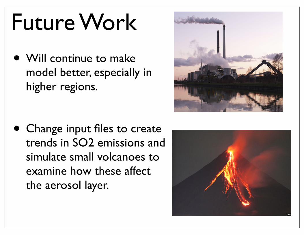
Future Work• Will continue to make

model better, especially in higher regions.

• Change input files to create trends in SO2 emissions and simulate small volcanoes to examine how these affect the aerosol layer.

global lidar remote sensing of stratospheric aerosols and

Documents