global ground strike point characteristics in negative

1

Global ground strike point characteristics in negative downward

lightning flashes ― part 1: Observations

Dieter R. Poelman1, Wolfgang Schulz2, Stephane Pedeboy3, Dustin Hill4, Marcelo Saba5, Hugh Hunt6,

Lukas Schwalt7, Christian Vergeiner7, Carlos Mata4, Carina Schumann6, and Tom Warner8

1Royal Meteorological Institute, Brussels, Belgium 5

2Austrian Lightning Detection and Information System (ALDIS), Vienna, Austria

3Météorage, Pau, France

4Scientific Lightning Solutions LLC (SLS), Titusville, Florida, USA

5National Institute for Space Research, INPE, São José dos Campos, Brazil

6The Johannesburg Lightning Research Laboratory, School of Electrical and Information Engineering, University of 10

Witwatersrand Johannesburg, Johannesburg, South Africa

7Institute of High Voltage Engineering and System Performance, Graz University of Technology, Graz, Austria

8ZT Research, Rapid City, South Dakota, USA

Correspondence to: Dieter R. Poelman ([email protected])

Abstract Lightning properties of a total of 1174 negative downward lightning flashes are analyzed. The high-speed video 15

recordings are taken in different regions around the world, including Austria, Brazil, South Africa and USA, and are

analyzed in terms of flash multiplicity, duration, interstroke intervals and ground strike point (GSP) properties. Although the

results vary among the data sets, the analysis reveals that a third of the flashes are single-stroke events, while the overall

mean number of strokes per flash equals 3.67. From the video imagery an average of 1.56 GSPs per flash is derived, with

about 60% of the multiple stroke flashes striking ground in more than one place. It follows that the channel creating a GSP is 20

re-used by a factor of 2.3. Multiple-stroke flashes last on average 371 ms, whereas the geometric mean (GM) interstroke

interval value preceding strokes producing a new GSP is about 18% greater than the GM value preceding subsequent

strokes following a pre-existing channel. In addition, a positive correlation between the duration and multiplicity of the flash

is presented. The characteristics of the subset of flashes exhibiting multiple GSPs is further examined. It follows that strokes

with stroke order of two create a new GSP in 60% of the cases, while this percentage quickly drops for higher order strokes. 25

Further, the possibility to form a new channel to ground in terms of the number of strokes that conditioned the previous

channel shows that approximately 88% developed after the occurrence of only one stroke. Investigating the time intervals in

the other 12% of the cases when two or more strokes re-used the previous channel showed that the average interstroke time

interval preceding a new channel is found to be more than twice the time difference between strokes that follow the previous

channel. 30

https://doi.org/10.5194/nhess-2021-12Preprint. Discussion started: 11 February 2021c© Author(s) 2021. CC BY 4.0 License.

2

1 Introduction

Cumulonimbus clouds are the birthplace of one of Earths’ true spectacles in nature: the lightning discharge. The

development of these clouds involves a number of steps. As the building phase comes to an end, characterized by a rapid

increase of growth of the clouds’ height through the rise of pockets of warm and moist air, it sets the stage for super cooled

cloud droplets to coagulate and increase in both mass and size. The subsequent mature phase provides the electric charge 35

structure through a range of collisions between the icy particles. Typically, this results in the top of the cloud being

predominantly positively charged, while the bottom of the cloud accomodates the bulk of the negatively charged particles. It

is at this magical moment, when eventually the difference in charge potential reaches a certain threshold, that the cloud

‘switches on the light’ and powerful electrical discharges appear, proudly drawing the attention of the spectator to an even

greater extent than was the case moments before. Followed by the dissipation phase, this gigantic wasteland of energy, once 40

capable of producing severe weather at ground, disappears and leaves us in awe.

Lightning radiates its energy in almost the full range of the electromagnetic spectrum. Hence, to observe and further increase

our understanding of lightning discharges in these cauliflower-like clouds, and the associated forces and physical processes

that are present within them, a whole range of instruments and techniques are at our disposal. The use of ground-based

lightning location systems (LLS), much in the same way compared to those constructed by todays’ standards, was first 45

introduced more than 40 years ago (Lewis et al., 1960; Krider et al., 1976). Present-day LLSs operate from very low

frequencies (VLF) and to very high frequencies (VHF) and are able to detect cloud-to-ground (CG) strokes and intracloud

(IC) pulses (e.g., Lay et al., 2004, Said et al., 2010; Gaffard et al, 2008; Zhu et al., 2017; Cummins et al., 1998; Schulz et al.,

2016; Thomas et al., 2004). Depending on the adopted technique, the total pathway covered by a lightning flash can be

presented as a single point or constitute several (even up to thousands of points) for a single discharge. Modern ground-based 50

low frequency LLSs are capable of differentiating between CG and IC flashes and tend to perform well in terms of flash and

stroke detection efficiencies, providing the location of downward CG ground strike points with high confidence.

On the other hand, satellite missions with onboard dedicated instruments provide a different way of capturing the

stroboscopical dance of lightning discharges by observing the scattered light peaking through the top of the cloud. The

signature of the strong optical oxygen triplet emission line at 777.4 nm is typically what is observed by means of specifically 55

designed cameras. Although first attempts started already from the 1970s (Vorpahl J.A. et al. 1970; Sparrow & Ney, 1971;

Turman, 1978), one had to wait until 1995 with the launch of the OV-1 (MicroLab 1) satellite with the onboard Optical

Transient Detector (OTD), closely followed by the Tropical Rainfall Measuring Mission (TRMM) carrying the Lightning

Imaging Sensor (LIS) in 1997, to witness the potential and significance of those type of missions. While the latter satellites

moved in a polar orbit around the Earth, the latest and future type of optical lightning instruments are being put in operation 60

from geostationairy orbit (Goodman et al., 2013;, Yang et al., 2017, Grandell et al., 2009), therewith expanding even further

the range of associated applications.


3

Even though its not uncommon to become lyrical about todays’ achievements in this field of research, the observations from

ground-based LLSs as well as from space have, besides governing many advantages, one fundamental drawback as it

observes the lightning discharge indirectly. Hence, the role of high-speed camera observations. Such observations gradually 65

dissect the flow of the electrical charged particles through the air and provide, linked to electric field measurements, a means

to investigate in great detail the associated optical and electromagnetic properties of natural downward lightning flashes.

With frame rates of 200 per second (fps) or more, the different strokes that compose a multi-stroke flash can each be

captured individually, while it is the electric field measurement that undisputably identifies the polarity of each stroke.

Furthermore, video imagery enable to determine, if not too distant and/or obscured by precipitation, whether each individual 70

stroke creates a new ground strike point (GSP) or follows a pre-existing channel (PEC). The characteristics deduced from

this is not only relevant from a pure scientific perspective, but is essential in developing adequate lightning protection

solutions as the level of lightning protection and risk to be mitigated is derived from the density of lightning terminations in

a region. Typically, this is based on flash density values but there have been recommendations to increase calculated

densities by a factor of two to account for multiple ground strike point flashes (Bouquegneau, 2013, 2014; IEC 62858, 75

2015). Understanding these characteristics is essential for evaluating whether such a factor is relevant.

In this paper, high-speed camera observations are analyzed in order to deduce some of the characteristics observed in natural

negative downward lightning flashes. Section 2 describes briefly the instrumentation used per region and analysis thereof is

provided in Section 3. Section 4 summarizes the findings of this study. In this context, it is worthwhile mentioning that the

data sets described here serve as basis to investigate the ability of so-called ground strike point algorithms to correctly group 80

strokes in flashes according to the observed ground strike points (Poelman et al., 2021, companion paper).

2 Data Acquisition and Analysis

Ground-truth campaigns are time consuming in order to gather enough data to be statistically relevant. To reach this

objective, ground-truth datasets are collected from different geographical regions and taken over various periods in time:

Austria (AT, EUCLID) in 2012, 2015, 2017 and 2018, Brazil (BR, RINDAT) in 2008, South Africa (SA, SALDN) in 2017-85

2019 and U.S.A. (US, NLDN) in 2015.

In this study, only flashes where a clear visible channel to the ground is observed for all the associated strokes are included.

However, it should be noted that even though such a selection of flashes is made, it does not undeniably resolve the true

contact point all of the time. This is certainly true when the observations are made at ground level. As such, the amount of

ground strike points retrieved from the video fields as discussed later on in this study should be regarded as a lower limit. In 90

the cases where the time interval between subsequent strokes is lower than 1 ms, the case is considered to be a forked stroke

rather than a stroke creating a new GSP, which in turn reduces the multiplicity of the flash. All the data sets, except US,

indicate the duration of the continuing current (CC) for each stroke if present in the recorded video fields.


4

In what follows, a description is given of the instrumentation set-up used at the different regions and the periods of

investigation. 95

2.1 Austria

A so-called video and field recording system (VFRS) is used to document lightning strikes in the alpine region of Austria.

The VFRS consists of a high-speed camera and an electric field measurement system and both are GPS time synchonized.

The system is composed of a flat plate antenna, an integrator and an amplifier, a fiber optic link, a digitizer and a PXI system

(Schulz et al., 2005). The camera used for the data recorded in 2015, 2017 and 2018 is the Vision Research Phantom V9.1, 100

operated at a frame rate of 2000 frames per second (fps), a 14-bit image depth and a resolution of 1248 × 400 pixels (Schulz

et al., 2009; Vergeiner et al., 2016, Schwalt, 2019, Schwalt et al., 2020) with a total record length of 1.6 s. In 2012 a

monochrome (8 bit per pixel) Basler camera was used at 200 frames per second with VGA resolution, i.e., 640x480 pixels,

and with a record length of 5 s.

2.2 Brazil 105

A Photron PCI-512 high-speed digital camera, operating at 4000 fps, was used to record the flashes in Southeastern Brazil in

2008. The high-speed video images are GPS time-stamped to an accuracy better than 1 millisecond with a 1 s pre-trigger

time and a total recording time of 2 s. Each trigger pulse was initiated manually by an operator when a flash was observed

within the camera field-of-view. For more details on the operation and accuracy of high-speed cameras for lightning

observations, see Saba et al. (2016). The polarity of the strokes is determined by matching the strokes to the observations of 110

a local lightning location system (LLS) BrasilDat in Brazil. More information on the characteristics of this network is given

by Naccarato and Pinto (2009).

2.3 South Africa

The high-speed study of lightning flashes over Johannesburg, South Africa began in 2017. Johannesburg is located in the

North Eastern province of Gauteng and sits at an altitude of approximately 1600m above sea level. The area has seasonal 115

thunderstorms, generally occurring during the mid-to-late afternoons in the summer months (September-April, Southern

Hemisphere) and with no thunderstorm activity during the winter months. The area has a flash density of 15 to 18

flashes/km2/year (Evert, 2017). The setup utilizes two high-speed cameras (a Phantom v7.1 and a Phantom v310) which are

located North-West of the city. Frame rates used are in the range of 5000 to 15000 fps and all captured videos are GPS time-

stamped. A one second buffer time is used and events are manually triggered. Note that in this area both downward and 120

upward events are captured. The latter are events triggered by the two tall towers located in Johannesburg – the Sentech and

Hillbrow tower, approximately 250m each (Schumann, 2018).


5

2.4 U.S.A.

The observations used in this study are taken from the Kennedy Space Center/Cape Canaveral Air Force Station

(KSC/CCAFS) in 2015. A compact network of 13 high-speed cameras record cloud-to-ground lightning return strokes 125

terminating on KSC/CCAFS property, with geographic emphasis on the areas surrounding Launch Complex 39B (LC-39B),

Launch Complex 39A (LC-39A), Launch Complex 41 (LC-41), and the Vehicle Assembly Building (VAB). Eight of the

cameras are located on tall structures at altitudes greater than 150m, providing downward vantage points. Many of the

cameras are configured with intersecting fields of view to provide multi-angle scenes of the same discharge. The high-speed

cameras sample at either 3,200 or 16,000 fps. The cameras have memory segment lengths ranging from about 100 ms to 400 130

ms and operate in segmented memory mode in order to capture many consecutive events without overrunning the internal

buffer. In this way, the entire sequence of strokes is captured over the full duration of a flash. In addition, six wideband rate

of change of electric field (dE/dt) sensors provide information on the polarity of the discharges. The digitization time bases

of these geographically independent sensors are synchronized with RMS accuracy of 15 ns.

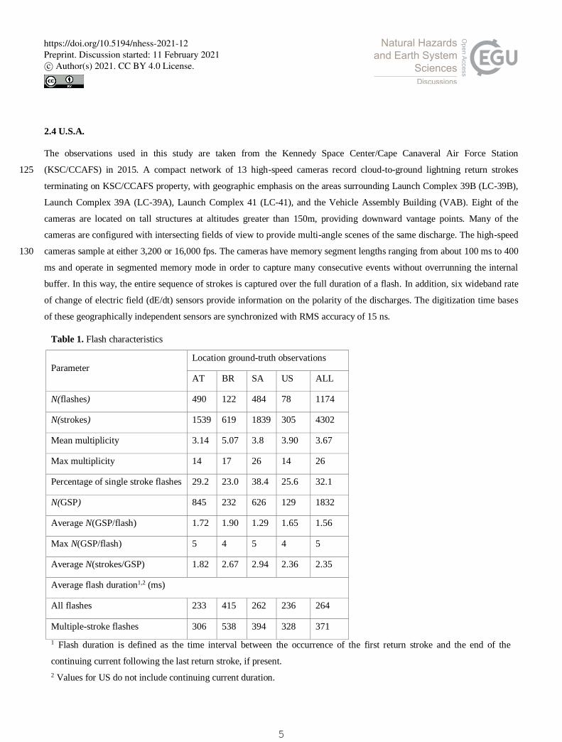
Table 1. Flash characteristics

Parameter Location ground-truth observations

AT BR SA US ALL

N(flashes) 490 122 484 78 1174

N(strokes) 1539 619 1839 305 4302

Mean multiplicity 3.14 5.07 3.8 3.90 3.67

Max multiplicity 14 17 26 14 26

Percentage of single stroke flashes 29.2 23.0 38.4 25.6 32.1

N(GSP) 845 232 626 129 1832

Average N(GSP/flash) 1.72 1.90 1.29 1.65 1.56

Max N(GSP/flash) 5 4 5 4 5

Average N(strokes/GSP) 1.82 2.67 2.94 2.36 2.35

Average flash duration1,2 (ms)

All flashes 233 415 262 236 264

Multiple-stroke flashes 306 538 394 328 371

1 Flash duration is defined as the time interval between the occurrence of the first return stroke and the end of the

continuing current following the last return stroke, if present.

2 Values for US do not include continuing current duration.

5


6

3. Results 135

The combined data sets comprise of 1174 flashes and 4302 strokes. The characteristics of each individual data set regarding

flashes, strokes, ground strike points, multplicity and flash duration are presented in Table 1. The largest data set in terms of

amount of flashes is the one of Austria with 490 flashes, closely followed by the South African data set containing 484

flashes. On the other hand, the data set of South Africa includes by far the largest amount of strokes. The distribution of the

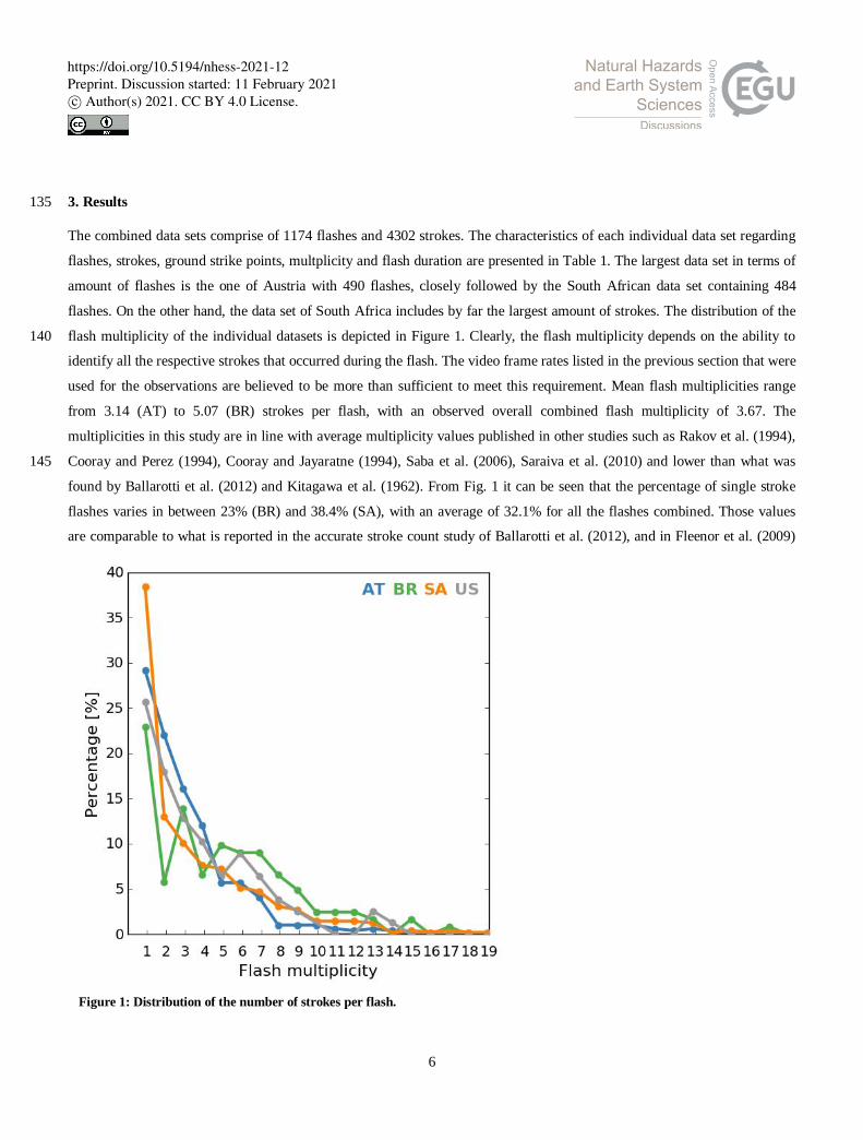
flash multiplicity of the individual datasets is depicted in Figure 1. Clearly, the flash multiplicity depends on the ability to 140

identify all the respective strokes that occurred during the flash. The video frame rates listed in the previous section that were

used for the observations are believed to be more than sufficient to meet this requirement. Mean flash multiplicities range

from 3.14 (AT) to 5.07 (BR) strokes per flash, with an observed overall combined flash multiplicity of 3.67. The

multiplicities in this study are in line with average multiplicity values published in other studies such as Rakov et al. (1994),

Cooray and Perez (1994), Cooray and Jayaratne (1994), Saba et al. (2006), Saraiva et al. (2010) and lower than what was 145

found by Ballarotti et al. (2012) and Kitagawa et al. (1962). From Fig. 1 it can be seen that the percentage of single stroke

flashes varies in between 23% (BR) and 38.4% (SA), with an average of 32.1% for all the flashes combined. Those values

are comparable to what is reported in the accurate stroke count study of Ballarotti et al. (2012), and in Fleenor et al. (2009)

Figure 1: Distribution of the number of strokes per flash.


7

150 and Biagi et al. (2006) based on standard video data. The value of the maximum multiplicity per data set is indicated in

Table 1 as well. One flash in SA stands out, containing a total of 26 strokes, while lasting 1.06 s.

As mentioned earlier, video observations allow classification of each stroke as a discharge creating either a new GSP, or

following a PEC. As such, a total of 1832 GSPs are resolved within the different data sets; yielding an average of 1.56 GSPs

per flash, while the mean amount of GSPs per flash for the different data sets ranges from 1.3 (SA) to 1.9 (BR). It follows 155

that the average number of lightning strike points is 56% higher than the number of flashes. This value is in line with those

reported in earlier studies such as the 1.45 strike points per CG flash observed in Tucson, Arizona, by Valine and Krider

(2002), 1.67 strike points per flash in Florida [Rakov et al., 1994], while in São Paulo, Brazil and in Arizona, US a value of

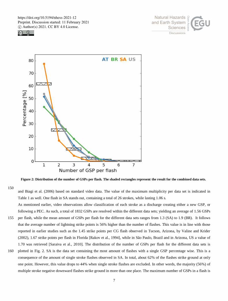
1.70 was retrieved [Saraiva et al., 2010]. The distribution of the number of GSPs per flash for the different data sets is

plotted in Fig. 2. SA is the data set containing the most amount of flashes with a single GSP percentage wise. This is a 160

consequence of the amount of single stroke flashes observed in SA. In total, about 62% of the flashes strike ground at only

one point. However, this value drops to 44% when single stroke flashes are excluded. In other words, the majority (56%) of

multiple stroke negative downward flashes strike ground in more than one place. The maximum number of GSPs in a flash is

Figure 2: Distribution of the number of GSPs per flash. The shaded rectangles represent the result for the combined data sets.


8

found to be 5, observed in Austria as well as in South Africa. Finally, adopting the values in Table 1 for the multiplicity and 165

average number of strike points for each data set, the average number of strokes observed per GSP varies between 1.82 (AT)

and 2.94 (SA). For all the data sets combined it turns out that a ground contact point is struck 2.35 times on average.

Figure 3 illustrates the duration of all the flashes in bins of 100 ms. The flash duration in this study is defined as the time

span between the first and last stroke in the flash, increased by the duration of an eventual continuing current (CC) following

the last stroke. Since the US data set does not contain information on the possible occurrence of CC, the plot is made 170

excluding US flashes. In addition, only multiple stroke flashes are included since many of the single stroke flashes were not

followed by any CC, therefore influencing the percentage of flashes that fall in the first duration bin. The mean and median

duration of multiple stroke flashes is found to be 371 ms and 313 ms, respectively. Ninety-five percent of the flashes have a

duration below 926 ms. The flash with the longest duration of 1379 ms is observed in SA for a six stroke flash and is in line

with the maximum flash duration values found in Saba et al. (2006) and Ballarotti et al. (2012). 175

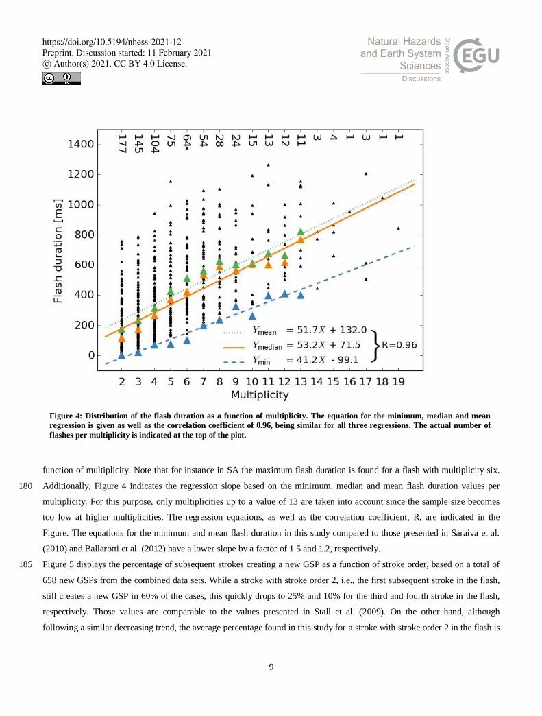
One can intuitively suppose that with increasing flash multiplicity, the flash duration increases accordingly. While this is in

general true, a large spread is observed in the data. This becomes apparent in Figure 4, which plots the flash duration as a

Figure 3: Distribution of the flash duration in bins of 100 ms. The actual number of flashes within each bin is listed above the bars.


9

function of multiplicity. Note that for instance in SA the maximum flash duration is found for a flash with multiplicity six.

Additionally, Figure 4 indicates the regression slope based on the minimum, median and mean flash duration values per 180

multiplicity. For this purpose, only multiplicities up to a value of 13 are taken into account since the sample size becomes

too low at higher multiplicities. The regression equations, as well as the correlation coefficient, R, are indicated in the

Figure. The equations for the minimum and mean flash duration in this study compared to those presented in Saraiva et al.

(2010) and Ballarotti et al. (2012) have a lower slope by a factor of 1.5 and 1.2, respectively.

Figure 5 displays the percentage of subsequent strokes creating a new GSP as a function of stroke order, based on a total of 185

658 new GSPs from the combined data sets. While a stroke with stroke order 2, i.e., the first subsequent stroke in the flash,

still creates a new GSP in 60% of the cases, this quickly drops to 25% and 10% for the third and fourth stroke in the flash,

respectively. Those values are comparable to the values presented in Stall et al. (2009). On the other hand, although

following a similar decreasing trend, the average percentage found in this study for a stroke with stroke order 2 in the flash is

Figure 4: Distribution of the flash duration as a function of multiplicity. The equation for the minimum, median and mean

regression is given as well as the correlation coefficient of 0.96, being similar for all three regressions. The actual number of

flashes per multiplicity is indicated at the top of the plot.


10

190 higher by about 10%-20% compared to what has been found previously in Rakov et al. (1994), Saba et al. (2006) and Ferro

et al. (2012).

It has been suggested by Rakov and Uman (1990) that the conditions after the first stroke in the flash are not favourable to

fully support the propagation of subsequent leaders all the way to the ground along the same path. Therefore, the stroke order

alone is not sufficient enough to predict the chance of creating a new GSP, as the full channels’ history needs to be taken into 195

account. The possibility to form a new channel to ground as a function of the number of strokes that conditioned the previous

channel is quantified in Figure 6. Out of a total of 658 new channels, 88.2% developed after the occurrence of only one

stroke, while this drops quickly to 7.6% and 2.6% in case of two and three observed consecutive strokes in the previous

channel, respectively. Note that in Austria two flashes are observed whereby a new GSP is created by the tenth stroke in the

flash, while the channel belonging to the previous GSP was used four and seven times, respectively. In the latter case, this 200

indicates that even after seven consecutive strokes within the same channel, it is still possible that the conditions to establish

an unalterable path to ground are not met or are simply ignored by a subsequent stroke. According to Ferro et al. (2012),

when two or more strokes have used the previous channel, then a larger interstroke time interval may be an important factor

in the creation of a new channel.

Figure 5: Distribution of the percentage of subsequent strokes creating a new GSP as a function of stroke order. The shaded rectangles represent the result for the combined data sets.


11

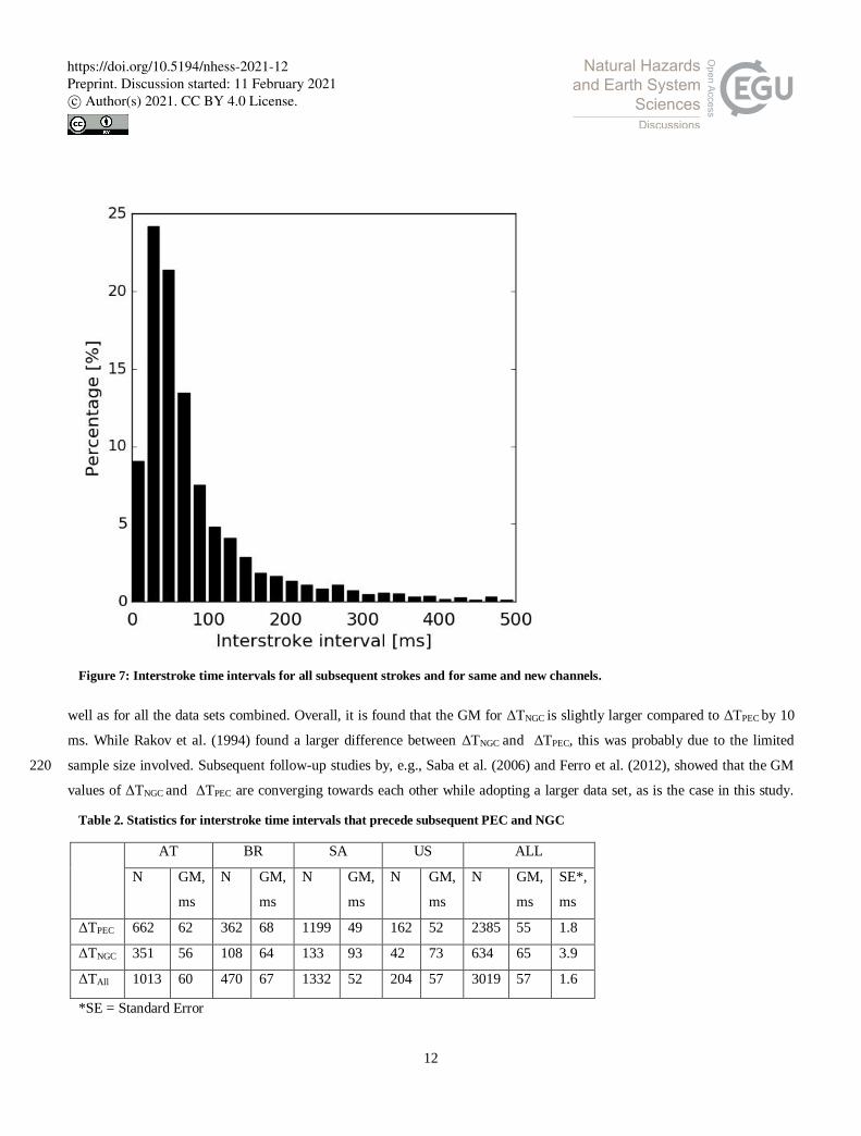
205 The distribution of 3128 time intervals is plotted in Figure 7 adopting a bin size of 20 ms and results thereof are listed in

Table 2. The average time interval is 85 ms, with a geometric mean (GM) of 57 ms. The maximum time interval for the

individual data sets is in the order of 500 ms to 700 ms, except for SA which contains a six-stroke flash with a maximum

observed time interval of 905 ms between the fifth and last stroke in the flash. Note that this particular flash is also the flash

with the maximum flash duration in all the data sets, and can be regarded as an exception, although time intervals well 210

exceeding 500 ms are recorded in other studies, e.g., Saba et al. (2006). Usually, these long time intervals between strokes

are due to a very long continuing current event following the first one. The 99th percentile appears to be 470 ms, somewhat

below the standard maximum interstroke time criterion of 500 ms usually adopted to group different strokes into flashes by

lightning location systems.

It is possible to further separate the interstroke time intervals from Figure 7 into intervals preceding strokes down the same 215

channel, ΔTPEC, or down a new channel, ΔTNGC. The results of this can be viewed in Table 2 for the individual data sets, as

Figure 6: Relation between new channel formation and the number of strokes in previous channel. The shaded

rectangles represent the result for the combined data sets.


12

well as for all the data sets combined. Overall, it is found that the GM for ΔTNGC is slightly larger compared to ΔTPEC by 10

ms. While Rakov et al. (1994) found a larger difference between ΔTNGC and ΔTPEC, this was probably due to the limited

sample size involved. Subsequent follow-up studies by, e.g., Saba et al. (2006) and Ferro et al. (2012), showed that the GM 220

values of ΔTNGC and ΔTPEC are converging towards each other while adopting a larger data set, as is the case in this study.

Figure 7: Interstroke time intervals for all subsequent strokes and for same and new channels.

Table 2. Statistics for interstroke time intervals that precede subsequent PEC and NGC

AT BR SA US ALL

N GM,

ms

N GM,

ms

N GM,

ms

N GM,

ms

N GM,

ms

SE*,

ms

ΔTPEC 662 62 362 68 1199 49 162 52 2385 55 1.8

ΔTNGC 351 56 108 64 133 93 42 73 634 65 3.9

ΔTAll 1013 60 470 67 1332 52 204 57 3019 57 1.6

*SE = Standard Error


13

There are some noticable differences among the individual data sets. While it is clear that ΔTNGC is considerably larger than

ΔTPEC in SA and US, the differences are much smaller or the opposite in the other data sets.

Some further investigation with respect to the time differences, analogous to Ferro et al. (2012) are presented in the 225

following. From Fig. 6 it is found that in 88% of the cases a new channel formation is observed after just one stroke in the

previous channel. Investigating now the time intervals in the other 12% of the cases when two or more strokes re-used the

previous channel, we find that the average interstroke time interval preceding a new channel becomes 77 ms, compared to a

time difference of 34 ms between strokes that follow the same channel, see Table 3. Therefore, in this subset of flashes,

ΔTNGC is about 2.3 times larger compared to ΔTPEC. This value is somewhat lower compared to the 3.5 times found in Ferro 230

et al. (2012), but still of the same order. Note that the interstroke time interval GM value for PEC strokes is in this case lower

by a factor of 1.6 compared to the result in Table 2.

4. Summary 235

Ground strike point characteristics in negative ground lightning flashes have been investigated by means of high-speed

camera observations taken in different parts around the globe. It is found that the mean amount of ground strike points per

flash is 1.56, while it varies from one place to the other. The values quoted in this study are in line with those found in the

literature, and reconfirms the necessity to take ground strike points into account to estimate the risk for lightning protection

purposes. While the number of flashes and strokes involved in this study is statistically relevant and, above all, larger 240

compared to any other similar study undertaken in the past, it remains a snapshot of that particular moment in time and

place. Consequently, it requires investigation in more detail of the regional and seasonal trends that might exist. In order to

overcome this, one could make use of the observations made by LLSs. Present day LLSs provide, with a high degree of

accuracy both in terms of efficiency and location, the different strokes that compose a flash. Ingesting those observations

into a so called ground strike point algorithm, in order to group individual strokes into ground strike points, would provide a 245

Table 3. Interstroke time interval between strokes using a PEC and interstroke time interval preceding a NGC after two or more strokes down the same channel

AT BR SA US combined

N [ms] N [ms] N [ms] N [ms] N [ms]

PEC 38 31 24 44 56 32 10 31 128 34

SE*[ms] 8.8 6.2 5.5 6.4 3.8

NGC 23 68 19 67 29 86 6 113 77 77

SE [ms] 15.3 15.6 33.7 19.2 14.4

*SE = Standard Error


14

means to study on a larger temporal and spatial scale the characteristics of ground strike point densities. The interested

reader is referred to Poelman et al. (2021, companion paper) to learn more about the ability of three such algorithms to

determine the observed ground strike points correctly based on the data set presented in this study.

The 99th percentile of the interstroke intervals is found to be 470 ms and certifies the commonly used maximum interstroke

interval of 500 ms to group strokes observed by a LLS into a flash while adopting a certain distance threshold. In addition, it 250

follows that the GM value for time intervals preceding the occurrence of a new channel is only slighlty larger than the

typical GM interstroke interval value of 57 ms. Overall, apart from a few exceptions, the total flash duration is below one

second and exhibits a positive correlation with the flash multiplicity.

In the majority of the cases, i.e., 88%, a new channel formation is observed after just one stroke in the previous channel.

This fact, together with the almost similar interstroke time intervals preceding strokes producing a NGC or following a PEC, 255

suggests that time interval alone is not enough to influence the creation of a new channel to ground. However, examining

the cases when two or more strokes re-used the previous channel, the average interstroke time interval preceding a new

channel is more than double the interval time between previous strokes that follow the same channel. This analysis

strengthens the outcome of Ferro et al. (2012).

Acknowledgments 260

HH and CS would like to thank the National Research Foundation of South Africa (Unique Grant No: 98244).

References

Ballarotti, M. G., Medeiros, C., Saba, M. M. F., Schulz, W., and O. Pinto Jr.: Frequency distributions of some parameters of

negative downward lightning flashes based on accurate-stroke-count studies, J. Geophys. Res., 117, D06112,

doi:10.1029/2011JD017135, 2012. 265

Biagi, C. J., Cummins, K. L., Kehoe, K. E., and Krider, E. P.: National Lightning Detection Network (NLDN) performance

in southern Arizona, Texas, and Oklahoma in 2003-2004, J. Geophys. Res., 112, D05208, doi:10.1029/2006JD007341, 2007

Bouquegneau, C., Lecomte, P., Coquelet, F., Poelman, D. and Crabbe, M. : Lightning flash and strike-point density in

Belgium, 8th Asia-Pacific International Conference on Lightning, 2013.

Bouquegneau, C.: The need for an international standard on Lightning Location Systems, 23rd International Lightning 270

Detection Conference, 2014.

Cooray, V., and Jayaratne, K. P. S. C.: Characteristics of lightning flashes observed in Sri Lanka in the tropics, J. Geophys.

Res., 99(D10),21,051–21,056, doi:10.1029/94JD01519, 1994.

Cooray, V., and Pérez, H.: Some features of lightning flashes observed in Sweden, J. Geophys. Res., 99(D5), 10,683–10,688,

doi:10.1029/93JD02366, 1994. 275


15

Cummins, K. L., Murphy, M. J., Bardo, E. A., Hiscox, W. L., Pyle, R. B., and Pifer, A. E., A combined TOA/MDF

technology upgrade of theU.S. National Lightning Detection Network, J. Geophys. Res., 103,9038 – 9044, 1998.

Evert, R.C and Gijben, M.: Official South African Lightning Ground Flash Density Map 2006 to 2017 – Earthing Africa

Inaugural Symposium and Exhibition, Johannesburg South Africa, 2017.

International Standard IEC 62858 Edition 1, lightning density based on lightning location systems (LLS) – General 280

principles, International Electrotechnical Commission, ISBN 978-2-8322-2820-3, 2015.

Ferro, M. A., Saba, M. M. F., and O. Pinto, Jr.: Time intervals between negative lightning strokes and the creation of new

ground terminations, Atmos. Res., 116, 130–133, 2012.

Fleenor, S. A., Biagi, C. J., Cummins, K. L., Krider, E. P., and Shao X.: Characteristics of cloud-to-ground lightning in

warm-season thunderstorms in the Central Great Plains, Atmospheric Research, 91, 333-352, 2009. 285

Gaffard, C., Nash, J., Atkinson, N., Bennett, A., Callaghan, G., Hibbett, E., Taylor, P., Turp, M., and Schulz, W.: Observing

lightning around the globe from the surface, in: the Preprints, 20th Interna tional Lightning Detection Conference, Tucson,

Arizona, 21–23, 2008.

Goodman, S. J., Blakeslee, R. J., Koshak, W. J., Mach, D., Bailey J., Buechler, D., Carey, L., Schultz, C., Bateman, M.,

McCaul, E., and Stano, G.: The GOES-R Geostationary Lightning Mapper (GLM), Atmospheric Research, 125-126, 34-49, 290

2013.

Grandell, J.; Finke, U.; Stuhlmann, R. The EUMETSAT meteosat third generation lightning imager (MTG-LI): Applications

and product processing. In Proceedings of the 9th EMS Annual Meeting, Toulouse, France, 28 September–2 October 2009.

Kitagawa, N., M. Brook, and E. J. Workman: Continuing currents in cloud-to-ground lightning discharges, J. Geophys. Res.,

67(2), 637–647, doi:10.1029/JZ067i002p00637, 1962. 295

Krider , E. P., Noggle, R. C., and Uman, M. A.: A gated wide-band magnetic direction finder for lightning return strokes. J.

Appl. Meteor., 15, 301-306, 1976.

Lay, E.H.; Holzworth, R.H.; Rodger, C.J.; Thomas, J.N.; Pinto, O., Jr.; Dowden, R.L. Source: WWLL global lightning

detection system: Regional validation study in Brazil, Geophysical Research Letters, v 31, n 3, 16 Feb. 5 pp., 2004.

Lewis, E. A., Harvey, R. B., and Rasmussen, J. E.: Hyperbolic direction finding with sferics of transatlantic origin, J. 300

Geophys. Res., vol. 65, pp. 1879–1905, 1960.

Naccarato, K. P., and O. Pinto, Jr.: Improvements in the detection efficiency model for the Brazilian lightning detection

network (Brasil- DAT), Atmos. Res., 91, 546–563, doi:10.1016/j.atmosres.2008.06.019, 2009.

Poelman, D. R., Schulz, W., Pedeboy, S., Campos, L. Z. S., Matsui, M., Hill, D., Saba, M., and Hunt, H.: Global ground

strike point characteristics in negative downward flashes – part 2: Algorithm validation, 2021, companion paper. 305

Rakov, V. A., and Uman, M. A.: Some properties of negative cloud- to-ground lightning, paper presented at 20th

International Conference on Lightning Protection, Swiss Electrotechn. Assoc., Interlaken, Switzerland, 1990.

Rakov, V. A., Uman, M. A., and Thottappillil, R., Review of lightning properties from electric field and TV observations, J.

Geophys. Res., 99, 10,745–10,750, doi:10.1029/93JD01205, 1994.


16

Saba, M. M. F., Ballarotti, M. G., Pinto Jr., O.: Negative cloud-to-ground lightning properties from high-speed video 310

observations. J. Geophys. Res. 111, D03101, doi:10.1029/2005JD006415, 2006.

Saba, M. M. F., Schumann, C., Warner, T. A., Ferro, M. A. S., de Paiva, A. R., J. Helsdon Jr, and Orville, R. E.: Upward

lightning flashes characteristics from high-speed videos, J. Geophys. Res. Atmos., 121, doi:10.1002/2016JD025137, 2016.

Said, R. K., Inan, U. S., and Cummins, K. L.: Long-range lightning geolocation using a VLF radio atmospheric waveform

bank, J. Geophys.Res., 115, D23108, doi:10.1029/2010JD013863, 2010. 315

Saraiva, A. C. V., Saba, M. M. F., Pinto, O., Cummins, K. L., Krider, E. P., and Campos, L. Z. S.: A comparative study of

negative cloud-to-ground lightning characteristics in São Paulo (Brazil) and Arizona (United States) based on high-speed

video observations, J. Geophys. Res., 115, D11102, doi:10.1029/2009JD012604, 2010.

Schulz, W., Lackenbauer, B., Pichler, H., Diendorfer, G.: LLS data and correlated continuous E-field measurements, SIPDA,

2005. 320

Schulz, W., and Saba, M.M.F.: First results of correlated lightning video images and electric field measurements in Austria,

SIPDA, 2009.

Schulz, W., Diendorfer, G., Pedeboy, S., and Poelman, D. R.: The European lightning location system EUCLID – Part 1:

Performance analysis and validation. Natural Hazards and Earth System Sciences, 16(2), 595–605.

https://doi.org/10.5194/nhess-16-595-2016, 2016. 325

Schumann, C., Hunt, H.G.P., Tasman, J., Fensham, H., Nixon, K.J., Warner, T.A., and Saba, M.M.F.: High-speed Video

Observation of Lightning Flashes Over Johannesburg, South Africa 2017 – 2018 International Conference on Lightning

Protection, 2018.

Schwalt, L.: Lightning Phenomena in the Alpine Region of Austria, Ph. D. thesis, Graz University of Technology, 147 pp.,

2019. 330

Schwalt, L., Pack, S., and Schulz, W.: Ground truth Data of Atmospheric Discharges in Correlation with LLS Detections,

Electric Power Systems Research Journal, 180, 2020.

Sparrow, J. G., and Ney, E. P.: Lightning observations by satellite. Nature, 232, 514–540, 1971.

Stall, C. A., Cummins, K. L., Krider, E. P., Cramer, J. A.: Detecting multiple ground contacts in cloud-to-ground lightning

flashes, J. Atmos. Oceanic Technol., 26 (11), 2392-2402, 2009. 335

Thomas, R. J., Krehbiel, P. R., Rison, W., Hunyady, S. J., Winn, W. P., Hamlin, T., and Harlin, J.: Accuracy of the

Lightning Mapping Array. Journal of Geophysical Research, 109, D14207. https://doi.org/10.1029/2004JD004549, 2004

Turman, B. N.: Analysis of lightning data from the DMSP satellite. Journal of Geophysical Research: Oceans, 83(C10),

5019–5024. https://doi.org/10.1029/JC083iC10p05019, 1978.

Valine, W., and Krider, E.P.: Statistics and characteristics of cloud-to-ground lightning with multiple ground contacts. J. 340

Geophys. Res., 107(D20), 4441, doi:10.1029/2001JD001360, 2002.

Vergeiner, C., Pack, S., Schulz, W., and Diendorfer, G.: Negative cloud-to-ground lightning in the alpine region: a new

approach, CIGRE International Colloquium, 2016.


17

Vorpahl J.A., Sparrow, J. G., and Ney, E. P.: Satellite observations of lightning. Science, 169, 860–862, 1970.

Yang, J., Zhang, Z., Wei, C., Lu, F., and Guo, Q.: Introducing the new generation of Chinese geostationary weather 345

satellites, Fengyun-4. Bull. Am. Meteorol. Soc. 2017, 98, 1637–1658, 2017.

Zhu, Y., Rakov, V. A., Tran, M. D., Stock, M. G., Heckman, S., Liu, C., …Hare, B. M.: Evaluation of ENTLN performance

characteristics based on the ground truth natural and rocket-triggered lightning data acquired in Florida. Journal of

Geophysical Research: Atmospheres, 122,9858–9866, https://doi.org/10.1002/2017JD027270, 2017.

350


global ground strike point characteristics in negative

Documents