Global Golub–Kahan bidiagonalization appliedto large discrete ill-posed problems

A. H. Bentbib

Laboratory LAMAI, FSTG, University of Cadi Ayyad, Marrakesh, Morocco.

M. El Guide

Laboratory LAMAI, FSTG, University of Cadi Ayyad, Marrakesh, Morocco.

K. Jbilou

Universite de Lille Nord de France, L.M.P.A, ULCO, 50 rue F. Buisson, BP699,

F-62228 Calais-Cedex, France.

L. Reichel

Department of Mathematical Sciences, Kent State University, Kent, OH 44242, USA.

Abstract

We consider the solution of large linear systems of equations that arise fromthe discretization of ill-posed problems. The matrix has a Kronecker prod-uct structure and the right-hand side is contaminated by measurement error.Problems of this kind arise, for instance, from the discretization of Fredholmintegral equations of the first kind in two space-dimensions with a separablekernel and in image restoration problems. Regularization methods, such asTikhonov regularization, have to be employed to reduce the propagation ofthe error in the right-hand side into the computed solution. We investi-gate the use of the global Golub–Kahan bidiagonalization method to reducethe given large problem to a small one. The small problem is solved byemploying Tikhonov regularization. A regularization parameter determinesthe amount of regularization. The connection between global Golub–Kahanbidiagonalization and Gauss-type quadrature rules is exploited to inexpen-sively compute bounds that are useful for determining the regularization

Email addresses: a.bentbib@uca.ma (A. H. Bentbib), medelguide@gmail.com (M.El Guide), jbilou@lmpa.univ-littoral.fr (K. Jbilou), reichel@math.kent.edu (L.Reichel)

Preprint submitted to Journal of Computational and Applied Mathematics (JCAM)April 16, 2018

parameter by the discrepancy principle.

Keywords: Global Golub–Kahan bidiagonalization, Ill-posed problems,Gauss quadrature.

1. Introduction

Linear ill-posed problems arise in essentially every branch of science andengineering, including in remote sensing, computerized tomography, and im-age restoration. Discretization of these problems gives rise to linear systemsof equations,

Hx = b, H ∈ RN×N , x, b ∈ RN , (1.1)

with a matrix that has many singular values of different orders of magnitudeclose to the origin; in particular, H may be singular. This makes the solutionx of (1.1), if it exists, very sensitive to perturbations in the right-hand sideb. In applications of interest to us, the vector b represents available data andis contaminated by an error e ∈ RN that may stem from measurement anddiscretization errors. Therefore, straightforward solution of (1.1), generally,does not yield a useful result.

Let b ∈ RN denote the unknown error-free vector associated with b, i.e.,

b = b+ e. (1.2)

We will assume the unavailable system of equations with error-free right-hand side,

Hx = b, (1.3)

to be consistent and denote its solution of minimal Euclidean norm by x.It is our aim to determine an accurate approximation of x by computingan approximate solution of the available linear system of equations (1.1).The first step in our solution process is to replace (1.1) by a nearby prob-lem, whose solution is less sensitive to the error e in b. This replacement iscommonly referred to as regularization. One of the most popular regular-ization methods is due to Tikhonov [7, 13]. In its simplest form, Tikhonovregularization replaces the linear system (1.1) by the minimization problem

minx∈RN

‖Hx− b‖22 + µ−1‖x‖22. (1.4)

Here µ > 0 is a regularization parameter and ‖ · ‖2 denotes the Euclideanvector norm. We will comment on the use of µ−1 instead of µ in (1.4) below.The minimization problem (1.4) has the unique solution

xµ := (HTH + µ−1IN )−1HT b (1.5)

2

for any fixed µ > 0. Here and throughout this paper IN denotes the identitymatrix of order N . The choice of µ affects how sensitive xµ is to the error ein b, and how accurately xµ approximates x. Many techniques for choosinga suitable value of µ have been analyzed and illustrated in the literature;see, e.g., [3, 7, 14, 21, 25] and references therein. In this paper we will usethe discrepancy principle. It requires that a bound ε for ‖e‖2 be availableand prescribes that µ > 0 be determined so that ‖b−Hxµ‖2 = ηε for a userchosen constant η ≥ 1 that is independent of ε; see [7, 14, 25] for discussionson this parameter choice method. In the present paper, we will determinea value µ > 0 such that

ε ≤ ‖b−Hxµ‖2 ≤ ηε, (1.6)

where the constant η > 1 is independent of ε.The computation of a µ-value such that the associated solution xµ of

(1.4) satisfies (1.6) generally requires the use of a zero-finder, see below,and typically ‖b − Hxµ‖2 has to be evaluated for several µ-values. Thiscan be expensive when the matrix H is large. A solution method based onfirst reducing H to a small bidiagonal matrix with the aid of Golub–Kahanbidiagonalization (GKB) and then applying the connection between GKBand Gauss-type quadrature rules to determine an approximation of xµ thatsatisfies (1.6) is discussed in [4].

It is the purpose of this paper to describe an analogous method for the

situation when H is the Kronecker product of two matrices, H1 = [h(1)i,j ] ∈

Rn×n and H2 ∈ Rm×m, i.e.,

H = H1 ⊗H2 =

h

(1)1,1H2 h

(1)1,2H2 · · · h

(1)1,nH2

h(1)2,1H2 h

(1)2,2H2 · · · h

(1)2,nH2

......

...

h(1)n,1H2 h

(1)n,2H2 · · · h

(1)n,nH2

∈ RN×N (1.7)

with N = mn. Then the GKB method can be replaced by the globalGolub–Kahan bidiagonalization (GGKB) method described by Toutounianand Karimi [26]. The latter method replaces matrix-vector product evalu-ations in the GKB method by matrix-matrix operations. It is well knownthat matrix-matrix operations execute efficiently on many modern comput-ers; see, e.g., Dongarra et al. [6]. Iterative methods based on the GGKBmethod therefore can be expected to execute efficiently on many computers.We will exploit the relation between Gauss-type quadrature rules and theGGKB method to determine a value µ and an associated approximation of

3

the vector xµ that satisfies (1.6). We remark that matrices H with a ten-sor product structure (1.7) arise in a variety of applications including whensolving Fredholm integral equations of the first kind in two space-dimensionswith a separable kernel, and in imaging restoration problems where the ma-trix H models a blurring operator. It is well known that many blurringmatrices have Kronecker structure (1.7) or can be approximated well by amatrix with this structure; see [19, 20, 27].

In applications of our solution method described in Section 5 both thematrices H1 and H2 are square. Then H is square. This simplifies thenotation and, therefore, only this situation will be considered. However,only minor modifications of the method are necessary to handle the situationwhen one or both of the matrices H1 and H2 are rectangular.

This paper continues our exploration of the application of global Krylovsubspace methods to the solution of large-scale problems (1.1) with a Kro-necker structure that was begun in [2]. There a scheme for computing anapproximation of x of prescribed norm is described. It was convenient tobase this scheme on the global Lanczos tridiagonalization method and use itsconnection to Gauss-type quadrature rules. The paper focuses on the morecommon situation that a bound for the norm of the error e in b is availableor can be estimated. Then the regularization parameter µ > 0 can be de-termined by the discrepancy principle, i.e., so that the computed solutionsatisfies (1.6); see [7, 14]. The requirement (1.6) on the computed solutionmakes it natural to apply the GGKB method to develop an analogue of theapproach in [4]. Timings and counts of arithmetic floating point operations(flops) show the structure-respecting method of the present paper to requireless computing time and fewer flops than than the structure-igoring methoddescribed in [4], while giving an approximate solution of about the samequality. There are presently no other available methods that exploit theKronecker structure and determine the regularization parameter µ by thediscrepancy principle.

This paper is organized as follows. Section 2 discusses how the Kroneckerproduct structure can be utilized when determining an approximate solutionof (1.4) with the aid of the GGKB method. The connection between theGGKB method and Gauss-type quadrature rules is reviewed in Section 3,and the application of the GGKB method and Gauss-type quadrature todetermine an approximate solution of (1.4) that satisfies (1.6) is describedin Section 4. Numerical examples are presented in Section 5 and concludingremarks can be found in Section 6.

4

2. Kronecker structure

Introduce the operator vec, which transforms a matrix A = [ai,j ] ∈ Rm×nto a vector a ∈ Rmn by stacking the columns of A from left to right, i.e,

a = [a1,1, a2,1, . . . , am,1, a1,2, a2,2, . . . , am,2, . . . , am,n]T . (2.1)

We also need the inverse operator, mat, which transforms a vector (2.1) toan associated matrix A = [ai,j ] ∈ Rm×n. Thus,

vec(A) = a, mat(a) = A.

The Kronecker product satisfies the following relations for matricesA,B,C,D,Xof suitable sizes,

(A⊗B)vec(X) = vec(BXAT ),

(A⊗B)T = AT ⊗BT ,

(AB)⊗ (CD) = (A⊗ C)(B ⊗D),

(2.2)

see, e.g., [17] for proofs. For matrices A,B ∈ Rm×n, we define the innerproduct

〈A,B〉F := tr(ATB),

where tr(·) denotes the trace, and we note that

〈A,B〉F = (vec(A))T vec(B).

The Frobenius norm is associated with this inner product,

‖A‖F := 〈A,A〉1/2F ,

and satisfies‖A‖F = ‖vec(A)‖2. (2.3)

Two matrices A,B ∈ Rm×n are said to be F -orthogonal if

〈A,B〉F = 0.

Let H1 and H2 be Kronecker factors of the matrix H, cf. (1.7), anddefine the linear operator

A : Rm×n → Rm×n

A(X) := H2XHT1 .

5

Its transpose is given by AT (X) := HT2 XH1. We will need the symmetric

linear operatorA(X) := (AT A)(X),

where denotes composition. It can be expressed as

A(X) = HT2 H2XH

T1 H1. (2.4)

Let B := mat(b) ∈ Rm×n and assume that G := AT (B) 6= O, whereO ∈ Rm×n denotes the zero matrix. Let 0 < µ <∞. Then the equation

(A+ µ−1Im)(X) = G (2.5)

has a unique solution Xµ ∈ Rm×n. Using (2.4) this equation can be writtenas

HT2 H2XH

T1 H1 + µ−1X = HT

2 BH1.

With the aid of (2.2), we can express the above equation in the form

((H1 ⊗H2)T (H1 ⊗H2) + µ−1IN )vec(X) = (H1 ⊗H2)T vec(B).

This equation is equivalent to the normal equations associated with (1.4).Therefore, Xµ = mat(xµ).

Proposition 2.1. Let 0 < µ < ∞ and let Xµ be the unique solution of(2.5). Introduce the function

φ(µ) := ||B −A(Xµ)||2F . (2.6)

Let η > 1 be the same as in (1.6). Then

ε2 ≤ φ(µ) ≤ η2ε2 (2.7)

is equivalent to that xµ = vec(Xµ) satisfies (1.6) with b = vec(B).

Proof. Using (2.3) and (2.2), in order, yields

φ(µ) = ‖B−H2XµHT1 ‖2F = ‖vec(B)−vec(H2XµH

T1 )‖22 = ‖b−(H1⊗H2)xµ‖22,

and the proposition follows from H = H1 ⊗H2. 2

The proposition implies that we can use Xµ instead of xµ when de-termining a value of µ such that (1.6) holds. We will apply the followingimplementation of the GGKB method to determine an approximation ofXµ. The GGKB method generates two sequences of F -orthogonal matricesas well as a bidiagonal matrix.

6

Algorithm 1: The GGKB method

1. Set σ1 = ||B||F , U1 = B/σ1, V1 = O

2. For j = 1, 2, . . . , k(a) Vj = AT (Uj)− σjVj(b) ρj = ‖Vj‖F(c) Vj = Vj/ρj(d) Uj+1 = A(Vj)− ρjUj(e) σj+1 = ||Uj+1||F(f) Uj+1 = Uj+1/σj+1

EndFor

The above algorithm determines the decompositions

Uk+1(σ1e1 ⊗ In) = B,[A(V1),A(V2), . . . ,A(Vk)

]= Uk+1(Ck ⊗ In),[

AT (U1),AT (U2), . . . ,AT (Uk)]

= Vk(CTk ⊗ In),

(2.8)

where ej = [1, 0, . . . , 0]T denotes the first axis vector. The matrix

Vk = [V1, V2, . . . , Vk] ∈ Rm×kn, Uk+1 = [U1, U2, . . . , Uk+1] ∈ Rm×(k+1)n,

have F -orthonormal “matrix columns” Vj ∈ Rm×n and Uj ∈ Rm×n, respec-tively, i.e.,

〈Vi, Vj〉F = 〈Ui, Uj〉F =

1 i = j,0 i 6= j.

Finally, the matrix Ck ∈ Rk×k is bidiagonal,

Ck =

ρ1

σ2 ρ2

. . .. . .

σk−1 ρk−1

σk ρk

(2.9)

and so is

Ck =

[Ck

σk+1eTk

]∈ R(k+1)×k.

We remark that the matrix columns U1, U2, U3, . . . , are only required toadvance the computations of Algorithm 1. Therefore, they all can be storedin the same memory location. Also, the matrix column Uj+1 can use thislocation. The matrix columns V1, V2, . . . , Vk will be used to determine an ap-proximate solution of (1.1) and, therefore, cannot be overwritten. However,the matrix columns Vj and Vj+1 may share the same storage location.

7

3. Gauss quadrature

This section discusses how the GGKB method is related to quadraturerules of Gauss-type. The connection follows via the relation between globalLanczos tridiagonalization and Gauss quadrature. Combining the equations(2.8) yields

[A(U1), A(U2), . . . , A(Uk)] = Uk(CkCTk ⊗ In) + σk+1[O, . . . , O, Uk+1], (3.1)

where O is a zero matrix. This decomposition also can be determined byapplying k steps of the global symmetric Lanczos (GSL) method to thematrix A with initial block vector B. The GSL method is described in[18] and its relation to Gauss quadrature is discussed in [2]. We thereforeonly provide an outline. We remark that the relation between the standardsymmetric Lanczos method and Gauss-type quadrature is well known; see,e.g., [4, 11, 12].

Proposition 3.1. Assume that HT b 6= 0. Then the function (2.6) can beexpressed as

φ(µ) = bT (µHHT + Imn)−2b. (3.2)

Proof. The proof of Proposition 2.1 shows that the function (2.6) can bewritten as

φ(µ) = ‖b−Hxµ‖22.

Substituting (1.5) into the right-hand side and using the identity, for µ > 0,

H(HTH + µ−1Imn)−1HT = Imn − (µHHT + Imn)−1 (3.3)

gives (3.2). 2

Substituting the spectral factorization HHT = WΛW T , where W ∈Rmn×mn is orthogonal and Λ = diag[λ1, λ2, . . . , λmn] ∈ Rmn×mn, into theright-hand side of (3.2) yields

φ(µ) =

mn∑j=1

fµ(λj)w2j . (3.4)

Here [w1, w2, . . . , wmn]T := W T b and

fµ(t) := (µt+ 1)−2.

The expression (3.4) is a Stieltjes integral, which we write as

φ(µ) =

∫fµ(t)dω(t). (3.5)

8

The distribution function ω associated with the measure dω can be chosenas a nondecreasing piecewise constant function with nonnegative jumps w2

j

at the eigenvalues λj . Since HHT is positive semidefinite, the support ofthe measure dω lives on the nonnegative real axis.

Define the integral

If :=

∫f(t)dω(t)

for suitable functions f and let Gk denote the k-point Gauss quadrature ruleassociated with dω. It is characterized by the property that

Gkp = Ip ∀p ∈ P2k−1,

where P2k−1 denotes the set of polynomials of degree at most 2k − 1. Theglobal Lanczos decomposition (3.1) provides a way to evaluate this Gaussrule without explicit knowledge of the measure dω. We have that for suitablefunctions f ,

Gkf = ‖B‖2F eT1 f(Tk)e1,

where the matrix Tk := CkCTk is symmetric and tridiagonal; see [2] for a

proof. Analogous results that relate standard Golub–Kahan bidiagonaliza-tion to Gauss quadrature have been shown by Golub and Meurant [11, 12]and are applied in [4]. Gautschi [10] provides a nice fairly recent discussionon Gauss quadrature and orthogonal polynomials; see also [9].

We are particularly interested in the Gauss rule

Gkfµ = ‖B‖2F eT1 (µCkCTk + Ik)

−2e1. (3.6)

Using the remainder formula for Gauss quadrature and the fact that alleven-order derivatives of the integrand t → fµ(t) in (3.5) are positive, onecan show that, generically,

G1fµ < · · · < Gk−1fµ < Gkfµ < φ(µ); (3.7)

see, e.g., [2, 23] for details.Let Rk+1 denote the (k+1)-point Gauss–Radau rule for the measure dω

with a fixed node t0 = 0. Then

Rk+1p = Ip ∀p ∈ P2k.

This rule, when applied to the integration of fµ, can be can expressed as

Rk+1fµ = ‖B‖2F eT1 (µCkCTk + Ik+1)−2e1;

9

see [2]. The remainder formula for Gauss–Radau quadrature rules and thefact that all odd-order derivatives of t → fµ(t) are negative yield that,generically,

φ(µ) < Rk+1fµ < Rkfµ < · · · < R1fµ; (3.8)

see, e.g., [2, 23].We conclude that pairs of Gauss and Gauss–Radau quadrature rules

Gkfµ and Rk+1fµ yield lower and upper bounds, respectively, for φ(µ). Weevaluate these rules by first executing Algorithm 1 and then solving theleast-squares problem

minz∈Rk

∥∥∥∥[µ1/2CTkIk

]z − ek+1

∥∥∥∥2

2

. (3.9)

The solution, denoted by zk, satisfies

(µCkCTk + Ik)zk = e1. (3.10)

It follows from (3.6) that

Gkfµ = ‖B‖2F zTk zk.

The special structure of the least-squares problem (3.9) makes it possibleto evaluate Gkfµ in only O(k) arithmetic floating-point operations for eachvalue of µ. Typically Gkfµ has to be evaluated for several µ-values; seeSection 4. The evaluation of Rk+1fµ can be carried out analogously; thematrix CTk in (3.9) has to be replaced by CTk ; see [2]. The reason for solvingthe least-squares problem instead of the associated normal equations (3.10)is that the solution of the former generally is less sensitive to errors in thedata and to round-off errors introduced during the computations.

4. Parameter selection and computation of an approximate solu-tion

This section describes how the bounds for φ(µ) described in the previoussection can be used to determine a suitable number of steps k of the GGKBmethod, a value µk of the regularization parameter, and an approximationxµk,k of the vector xµk , defined by (1.5) with µ = µk, that satisfies (1.6).

For a given value of k ≥ 2, we solve the nonlinear equation

Gkfµ = ε2 (4.1)

10

for µ. Because we use the parameter µ in (1.4), instead of 1/µ, the left-handside is a decreasing convex function of µ. There is a unique solution, denotedby µε, of

φ(µ) = ε2 (4.2)

for almost all values of ε > 0 of practical interest and therefore also of(4.1) for k sufficiently large; see [2, 4] for analyses. Various zero-finders canbe applied, including Newton’s method; see [22]. The evaluation of eachiterate requires the solution of a least-squares problem (3.9). The followingresult shows that the regularization parameter determined by solving (4.1)provides more regularization than the parameter obtained by solving (4.2).

Proposition 4.1. Let µk solve (4.1) and let µε solve (4.2). Then, generi-cally, µk < µε.

Proof. It follows from (3.2) that φ(µ) is a decreasing and convex functionfor µ ≥ 0 with φ(0) = ‖b‖22. Similarly, by (3.6), Gkfµ is a decreasing andconvex function for µ ≥ 0 with Gkf0 = ‖b‖22. Generically, φ(µ) > Gkfµ forµ > 0; cf. (3.7). Therefore, typically, µk < µε. We have equality in therare event of breakdown of the recursion formulas for the GGKB method.Assume that the ρk > 0 in (2.9). Then the matrix (2.9) is nonsingular andthe solution µk of (4.1) exists if 0 < ε < ‖b‖2. Let PN (HHT ) denote the

orthogonal projector onto the null space of HHT . Then the solution µε of(4.2) exist if ‖PN (HHT )b‖2 < ε < ‖b‖2. 2

Having computed µk, we check whether

Rk+1fµ ≤ η2ε2 (4.3)

holds for µ = µk. If this is the case, then it follows from (3.7) and (3.8)that (2.7) is valid for µ = µk. If, on the other hand, the inequality (4.3) isviolated for µ = µk, then we increase k by one, compute µk+1, and checkwhether (4.3) holds with k + 1 replaced by k + 2 for µ = µk+1. For mostproblems of interest, the Gauss and Gauss-Radau approximations (3.7) and(3.8) converge quite rapidly to φ(µk) as k increases. Therefore, the bound(4.3) typically holds already for a fairly small value of k.

Assume that µk satisfies (4.1) and (4.3). Then we determine an approxi-mate solution of (1.4) with the aid of the global Golub–Kahan decomposition(2.8) as follows. First we determine the solution yk,µk of

(CTk Ck + µ−1k Ik)y = σ1C

Tk e1, σ1 = ‖B‖F . (4.4)

11

It is computed by solving the least-squares problem

miny∈Rk

∥∥∥∥∥[µ

1/2k CkIk

]k

y − σ1µ1/2k e1

∥∥∥∥∥2

.

Similarly as above, we solve this least-squares problem instead of the asso-ciated normal equations (4.4) because of the better numerical properties ofthe latter. Finally, our approximate solution of (2.5) is determined by

Xk,µk = Vk(yk,µk ⊗ In). (4.5)

Proposition 4.2. The approximate solution (4.5) of (2.5) satisfies

ε ≤ ‖B −A(Xk,µk)‖F ≤ ηε. (4.6)

Proof. Using the representation (4.5), and applying (2.8) as well as (2.2),shows that

A(Xk,µk) = Uk+1(Ck ⊗ In)(yk,µk ⊗ In) = Uk+1(Ckyk,µk ⊗ In).

Substituting the above expression into (4.6) and again using (2.8) yields

‖Uk+1(σ1e1 ⊗ In)− Uk+1(Ckyk,µk ⊗ In)‖2F= ‖(σ1e1 ⊗ In)− (Ckyk,µk ⊗ In)‖2F= ‖σ1e1 − Ckyk,µk‖

22,

where we recall that σ1 = ‖B‖F . We now express yk,µk with the aid of (4.4),and apply the identity (3.3) with H replaced by Ck, to obtain

‖B −A(Xk,µk)‖2F= σ2

1‖e1 − Ck(CTk Ck + µ−1k Ik)

−1CTk e1‖22= σ2

1eT1 (µkCkC

Tk + Ik+1)−2e1

= Rk+1fµk .

The proposition now follows from (4.3) and the fact that ε2 = Gkfµk ≤Rk+1fµk . 2

The following algorithm summarizes the computation of (4.5).

12

Algorithm 2. The GGKB-Tikhonov method

Input: H1, H2, B, ε, η ≥ 1

1. Set k = 2 (k is the number of global Lanczos steps.)Let U1 := B/||B||F ;

2. Determine the F -orthonormal bases Ujkj=1 and Vjkj=1, and the

bidiagonal matrices Ck and Ck with Algorithm 1.

3. Determine µk that satisfies (4.1) and (4.3) as described above. Thismay require k to be increased, in which case one returns to step 2.

4. Determine yk,µk and Xk,µk as described above.

We comment on the complexity of Algorithm 2. First note that the overallcomputational cost for Algorithm 2 is dominated by the work required todetermine Uj and Vj at step 2 (here we ignore the computational cost ofevaluating AT (Uj) and A(Vj) in Algorithm 1). The computational effortrequired to determine Uj and Vj is dominated by the evaluation of fourmatrix-matrix products, which demands approximately 4(m + n)N flops.These matrix-matrix operations need fewer flops than structure-ignoringevaluation of matrix-vector products with the large matrix H and its trans-pose, which requires approximately 4N2 flops.

5. Numerical examples

This section presents a few representative numerical experiments. Allcomputations were carried out using the MATLAB environment on an In-tel(R) Core (TM) 2 Duo CPU T5750 computer with 3 GB of RAM. Thecomputations were done with approximately 15 decimal digits of relativeaccuracy.

Let x := vec(X) denote the error-free exact solution of the linear systemof equations (1.1), let B := H2XH

T1 and B := B + E, and define

b := vec(B), b := vec(B), e := vec(E),

where the error matrix E has normally distributed entries with zero meanand is normalized to correspond to a specific noise level

ν :=||E||F||B||F

.

The sizes of the matrices is specified in the examples below.

13

To determine the effectiveness of our solution method, we evaluate therelative error

||X −Xk||F||X||F

of the computed approximate solution Xk = Xk,µk determined by Algorithm2. The first three examples are concerned with the solution of Fredholmintegral equations of the first kind in two space-dimensions with a separablekernel. Discretization gives matrices that are severely ill-conditioned. Thelast two examples discuss image restoration problems. Overviews of imagerestoration problems can be found in [5, 16].

Example 1.

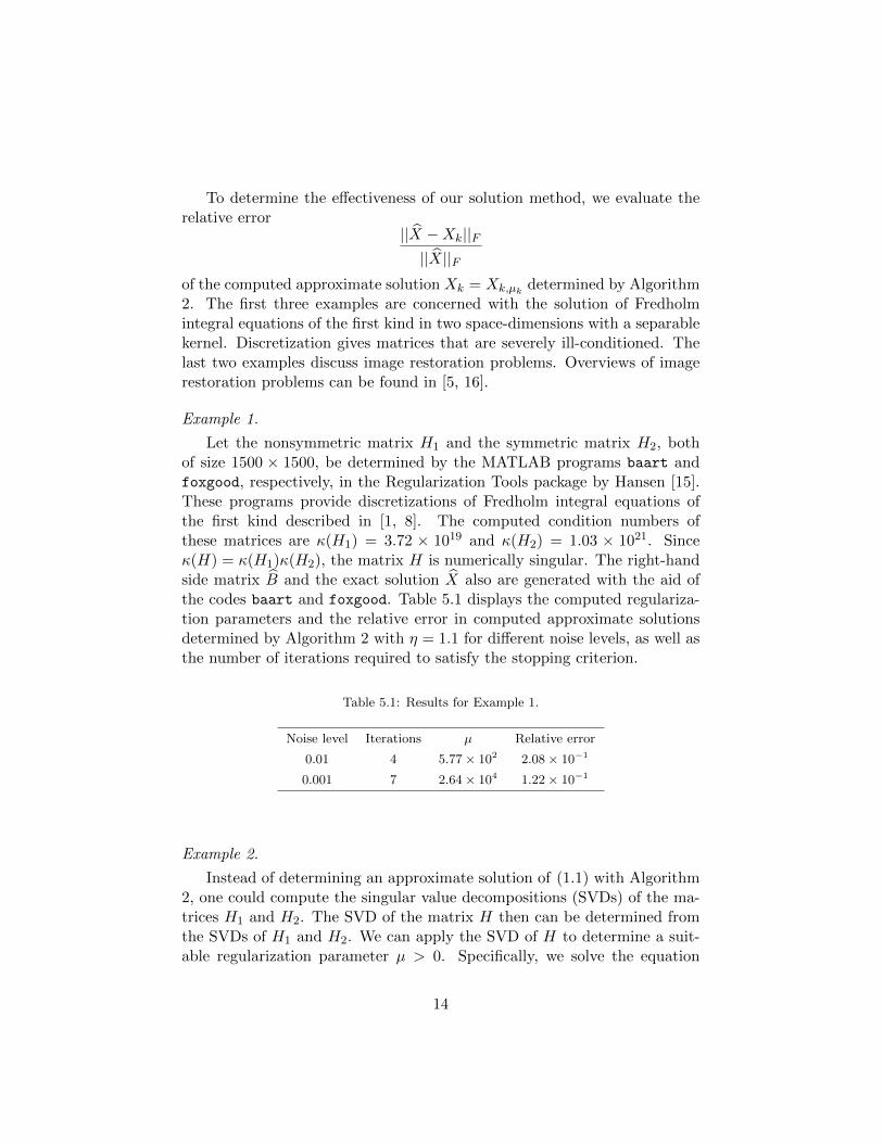
Let the nonsymmetric matrix H1 and the symmetric matrix H2, bothof size 1500 × 1500, be determined by the MATLAB programs baart andfoxgood, respectively, in the Regularization Tools package by Hansen [15].These programs provide discretizations of Fredholm integral equations ofthe first kind described in [1, 8]. The computed condition numbers ofthese matrices are κ(H1) = 3.72 × 1019 and κ(H2) = 1.03 × 1021. Sinceκ(H) = κ(H1)κ(H2), the matrix H is numerically singular. The right-handside matrix B and the exact solution X also are generated with the aid ofthe codes baart and foxgood. Table 5.1 displays the computed regulariza-tion parameters and the relative error in computed approximate solutionsdetermined by Algorithm 2 with η = 1.1 for different noise levels, as well asthe number of iterations required to satisfy the stopping criterion.

Table 5.1: Results for Example 1.

Noise level Iterations µ Relative error

0.01 4 5.77× 102 2.08× 10−1

0.001 7 2.64× 104 1.22× 10−1

Example 2.

Instead of determining an approximate solution of (1.1) with Algorithm2, one could compute the singular value decompositions (SVDs) of the ma-trices H1 and H2. The SVD of the matrix H then can be determined fromthe SVDs of H1 and H2. We can apply the SVD of H to determine a suit-able regularization parameter µ > 0. Specifically, we solve the equation

14

‖b−Hxµ‖2 = ηε for µ by Newton’s method without explicitly forming thematrices in the SVD of H. Knowing µ allows us to compute the Tikhonovsolution (1.5) without explicitly forming the matrices in the SVD of H.This approach of determining the regularization parameter and computingthe corresponding regularized solution (1.5) is attractive due to its simplicitywhen the matrices H1 and H2 are small. However, the approach is slow forlarge matrices H1 and H2. To illustrate this, we solve the same problem asin Example 1 with a finer discretization. Thus, let H1, H2 ∈ R2000×2000 bedetermined by the MATLAB codes baart and foxgood, respectively, from[15]. The matrices B and X are generated in the same manner as in Exam-ple 1 with the matrix B such that the noise level is ν = 0.01. We let thesafety factor for the discrepancy principle be η = 1.1. Then Algorithm 2 ter-minates after 4 iterations with the regularization parameter µ4 = 5.77× 102

and an approximate solution, defined by (4.5) with k = 4, with relative error2.09× 10−1. The computing time for this experiment is 37.96 seconds.

When we instead use the SVD of H, we obtain the regularization param-eter µ = 22.8 and an approximate solution with relative error 2.14 × 10−1.The computing time for this method is 47.95 seconds. The difference in thevalues of the regularization parameter for these approaches depends on thatin Algorithm 2 the regularization parameter is determined for the solutionin a subspace of low dimension, while the solution determined by the SVDapproach lives in the whole space.

The computations of this example illustrate that the computations withthe global Golub–Kahan method are faster than using the SVD of H, evenwhen the structure of the latter is exploited. The difference in computingtime is even more pronounced for larger problems. We remark that alsofor problems of the size considered in Example 1, the global Golub–Kahanmethod is faster than using the SVD of H.

Example 3.

We consider the Fredholm integral equation∫ ∫ΩK(x, y, s, t)f(s, t)dsdt = g(x, y), (x, y) ∈ Ω, (5.1)

where Ω = [−π/2, π/2]× [−π/2, π/2]. The kernel is given by

K(x, y, s, t) = k(x, s)k(y, t), (x, y), (s, t) ∈ Ω,

where

k(s, x) = (cos(s) + cos(x))2(sin(ξ)/ξ)2, ξ = π(sin(s) + sin(x)).

15

Figure 5.1: Example 3: Approximation X13 of X determined by Algorithm 2 for noiselevel 0.01.

The solution is the sum of two Gaussians in each space dimension.We discretize (5.1) by a Nystrom method based on the composite trape-

zoidal rule with equidistant nodes in each space-dimension. Code is avail-able at [24]. Specifically, we determine the nonsymmetric matrix H1 ∈R1500×1500, from which we obtain the discretization H = H1 ⊗ H1 of theintegral operator (5.1), as well as the exact solution X ∈ R1500×1500 of thediscretized problem and the associated exact right-hand side B. Table 5.2shows the computed regularization parameters and the relative error in ap-proximate solutions determined by Algorithm 2 with η = 1.01 and differentnoise levels, as well as the number of iterations required to satisfy the stop-ping criterion. Figure 5.1 displays the computed approximate solution X13

obtained when the noise level of the available data (right-hand side) is 0.01.

Table 5.2: Results for Example 3.

Noise level Iterations µ Relative error

0.01 13 2.46× 102 1.59× 10−1

0.001 32 2.67× 104 6.97× 10−2

16

Example 4.

This and the following examples are concerned with the restoration ofimages that have been contaminated by blur and noise. Let the entries ofthe vector x be pixel values for a desired, but unknown, image. The matrixH is a discretization of a blurring operator and equation (1.3) shows that brepresents a blurred, but noise-free, image. The vector b in (1.2) representsthe available blur- and noise-contaminated image associated with x. Theblurring matrix H is determined by a point-spread function (PSF), whichdetermines how each pixel is smeared out (blurred), and by the boundaryconditions, which specify our assumptions on the scene just outside theavailable image; see [5, 16] for details.

In some cases the horizontal and vertical components of the PSF canbe written as a product of two functions, one depending on the horizon-tal coordinate and the other one on the vertical coordinate, only. In thissituation, the blurring matrix H can be expressed as a Kronecker productH = H1 ⊗ H2. Let the matrix X = mat(x) be of suitable size. Then theblurred image can be represented as H2XH

T1 ; cf. (2.2). The blur- and noise-

contaminated image is represented by the matrix H2XHT1 + E, where E is

the noise matrix. Also when H cannot be written as a Kronecker product oftwo matrices, it may be possible to approximate H well by such a Kroneckerproduct; see [19, 20, 27].

In this example, we seek to restore an image that has been contaminatedby blur that is defined by a Gaussian PSF,

hσ(x, y) =1

2πσ2exp(− x2 + y2

2σ2

),

and by noise. The Dirichlet zero boundary condition is imposed. The blur-ring matrix then is the Kronecker product of a symmetric Toeplitz matriceswith itself H = H1 ⊗H1, where H1 = [hij ] with

hij =

1

σ√

2πexp

(− (i−j)2

2σ2

), |i− j| ≤ r,

0 else

The matrix H models atmospheric turbulence blur. We let σ = 2.5 andr = 6.

The original image X ∈ R256×256 is the Enamel image from MATLAB.It is shown in the left-hand side of Figure 5.2. The associated blurred andnoisy image B := H2XH

T1 + E is shown in the middle of Figure 5.2; the

noise level is 0.001. The restoration determined by Algorithm 2 with η = 1.1is displayed in the right-hand side of the figure.

17

Figure 5.2: Example 4: Original image (left), degraded image (center), and restored image(right) for noise of level 0.001.

For comparison, we determine a regularization parameter and an approx-imate solution using the numerical method described in [4]. This methoduses (standard) Golub–Kahan bidiagonalization instead of global Golub–Kahan bidiagonalization, and explores the connection between (standard)Golub–Kahan bidiagonalization and Gauss quadrature rules for solving largeill-conditioned linear systems of equations (1.1) without exploiting the struc-ture of the matrix H. We refer to this method as GKB in Table 5.3. Thetable compares results obtained by Algorithm 2 and GKB, including the rel-ative errors of the restorations, the number of iterations, and the CPU timesrequired for two noise levels. Algorithm 2 is seen to require less CPU timethan GKB and give about the same quality of the computed restoration asGKB.

Table 5.3: Results for Example 4.

Noise level Iterations Method µ Relative error CPU-time (sec)

0.0114 Algorithm 2 4.66× 103 1.02× 10−1 0.50

14 GKB 4.66× 103 1.02× 10−1 1.35

0.00162 Algorithm 2 1.71× 104 8.00× 10−2 2.23

62 GKB 1.71× 104 8.02× 10−2 11.44

Example 5.

The original image is the iograyBorder image of dimension 256 × 256from MATLAB. It is shown on the left-hand side of Figure 5.3. The blurring

18

Figure 5.3: Example 5: Original image (left), degraded image (center), and restored image(right) for noise of level 0.01.

matrix H = H1 ⊗H2 is the same as in Example 3. The blurred and noisyimage shown in the middle of Figure 5.3 has noise level 0.01. The restoredimage determined with Algorithm 2 with η = 1 is shown in the right-handside of Figure 5.3. The number of iterations, relative errors of the restoredimages, and computed regularization parameters are shown in Table 5.4 fortwo noise levels.

Table 5.4: Results for Example 5.

Noise level Iterations µ Relative error CPU time (sec)

0.01 19 4.80× 104 8.85× 10−2 1.09

0.001 75 2.60× 104 7.58× 10−2 2.13

6. Conclusion

This paper describes an iterative scheme based on the global Golub–Kahan bidiagonalization method for the approximate solution of the Tikhonovminimization problem (1.4) when the matrix H has a Kronecker structure.The method exploits the relation between global Golub–Kahan bidiagonal-ization and Gauss-type quadrature to inexpensively determine the regular-ization parameter so that the discrepancy principle is satisfied. The Kro-necker structure makes it possible to replace matrix-vector product evalua-tions in the scheme [4] by matrix-matrix product computations. The latterproducts execute more efficiently than the former on many computers.

19

References

[1] M. L. Baart, The use of auto-correlation for pseudo-rank determi-nation in noisy ill-conditioned least-squares problems, IMA J. Numer.Anal., 2 (1982), pp. 241–247.

[2] A. H. Bentbib, M. El Guide, K. Jbilou, and L. Reichel, Aglobal Lanczos method for image restoration, J. Comput. Appl. Math.,300 (2016), pp. 233–244.

[3] C. Brezinski, G. Rodriguez, and S. Seatzu, Error estimates forthe regularization of least squares problems, Numer. Algorithms, 51(2009), pp. 61–76.

[4] D. Calvetti and L. Reichel, Tikhonov regularization of large linearproblems, BIT, 43 (2003), pp. 263–283.

[5] B. Chalmond, Modeling and Inverse Problems in Image Analysis,Springer, New York, 2003.

[6] J. J. Dongarra, I. S. Duff, D. C. Sorensen, and H. A. van derVorst, Numerical Linear Algebra for High-Performance Computers,SIAM, Philadelphia, 1998.

[7] H. W. Engl, M. Hanke, and A. Neubauer, Regularization of In-verse Problems, Kluwer, Dordrecht, 1996.

[8] L. Fox and E. T. Goodwin, The numerical solution of non-singularlinear integral equations, Philos. Trans. R. Soc. Lond. Ser. A, Math.Phys. Eng. Sci., 245:902 (1953), pp. 501–534.

[9] W. Gautschi, The interplay between classical analysis and (numeri-cal) linear algebra – a tribute to Gene H. Golub, Electron. Trans. Nu-mer. Anal., 13 (2002), pp. 113–147.

[10] W. Gautschi, Orthogonal Polynomials: Approximation and Compu-tation, Oxford University Press, Oxford, 2004.

[11] G. H. Golub and G. Meurant, Matrices, moments and quadrature,in Numerical Analysis 1993, D. F. Griffiths and G. A. Watson, eds.,Longman, Essex, 1994, pp. 105–156.

[12] G. H. Golub and G. Meurant, Matrices, Moments and Quadraturewith Applications, Princeton University Press, Princeton, 2010.

20

[13] C. W. Groetsch, The Theory of Tikhonov Regularization for Fred-holm Integral Equations of the First Kind, Pitman, Boston, 1984.

[14] P. C. Hansen, Rank-Deficient and Discrete Ill-Posed Problems, SIAM,Philadelphia, 1998

[15] P. C. Hansen, Regularization tools version 4.0 for MATLAB 7.3, Nu-mer. Algorithms, 46 (2007), pp. 189–194.

[16] P. C. Hansen, J. G. Nagy, and D. P. O’Leary, Deblurring Images:Matrices, Spectra, and Filtering, SIAM, Philadelphia, 2006.

[17] R. A. Horn and C. R. Johnson, Topics in Matrix Analysis, CambridgeUniversity Press, Cambridge, 1991.

[18] K. Jbilou, H. Sadok, and A. Tinzefte, Oblique projection meth-ods for linear systems with multiple right-hand sides, Electron. Trans.Numer. Anal., 20 (2005), pp. 119–138.

[19] J. Kamm and J. G. Nagy, Kronecker product and SVD approxi-mations in image restoration, Linear Algebra Appl., 284 (1998), pp.177–192.

[20] J. Kamm and J. G. Nagy, Kronecker product approximations forrestoration image with reflexive boundary conditions, SIAM J. MatrixAnal. Appl., 25 (2004), pp. 829–841.

[21] S. Kindermann, Convergence analysis of minimization-based noiselevel-free parameter choice rules for linear ill-posed problems, Electron.Trans. Numer. Anal., 38 (2011), pp. 233–257.

[22] J. Lampe, L. Reichel, and H. Voss, Large-scale Tikhonov regular-ization via reduction by orthogonal projection, Linear Algebra Appl.,436 (2012), pp. 2845–2865.

[23] G. Lopez Lagomasino, L. Reichel, and L. Wunderlich, Ma-trices, moments, and rational quadrature, Linear Algebra Appl., 429(2008), pp. 2540–2554.

[24] A. Neuman, L. Reichel, and H. Sadok, Algorithms for range re-stricted iterative methods for linear discrete ill-posed problems, Numer.Algorithms, 59 (2012), pp. 325–331. Code is available in Netlib athttp://www.netlbib.org/numeralgo/ in the package na33.

21

[25] L. Reichel and G. Rodriguez, Old and new parameter choice rulesfor discrete ill-posed problems, Numer. Algorithms, 63 (2013), pp. 65–87.

[26] F. Toutounian and S. Karimi, Global least squares method (Gl-LSQR) for solving general linear systems with several right-hand sides,Appl. Math. Comput., 178 (2006), pp. 452–460.

[27] C. F. Van Loan and N. P. Pitsianis, Approximation with Kroneckerproducts, in Linear Algebra for Large Scale and Real Time Applications,M. S. Moonen and G. H. Golub, eds., Kluwer, Dordrecht, 1993, pp.293–314.

22