global distribution of solid and aqueous sulfate aerosols...

Global distribution of solid and aqueous sulfate aerosols:

Effect of the hysteresis of particle phase transitions

Jun Wang,1,2 Andrew A. Hoffmann,1 Rokjin J. Park,1,3 Daniel J. Jacob,1

and Scot T. Martin1

Received 9 September 2007; revised 14 February 2008; accepted 14 March 2008; published 10 June 2008.

[1] The partitioning between solid and aqueous phases of tropospheric sulfate-ammoniumparticles is simulated with a global 3-D chemical transport model (CTM). The simulationexplicitly accounts for the hysteresis of particle phase transitions by transportingaqueous sulfate and three solid sulfate forms (namely, ammonium sulfate, letovicite, andammonium bisulfate). Composition-dependent deliquescence relative humidities (DRH)and crystallization relative humidities (CRH) are based on recent laboratory data. We findthat the solids mass fraction on a sulfate basis is 0.34, partitioned as 93% ammoniumsulfate, 6% letovicite, and 1% ammonium bisulfate. The fraction increases with altitudefrom 0.10 to 0.30 in the boundary layer to 0.60–0.80 in the upper troposphere. Thedominance of solids in the upper troposphere arises in part from high sulfateneutralization, reflecting in our simulation a low retention efficiency of NH3 upon cloudfreezing. High sulfate neutralization is consistent with the few available observationsin the upper troposphere. High acidity with a dominant aqueous phase, however, can occurfollowing volcanic eruptions. Seasonal variation of the solids mass fraction in both thelower and upper troposphere is modulated by emissions of NH3 from the terrestrialbiosphere and biomass burning as well as by emissions of dimethylsulfide from the oceanbiosphere. The timescale of phase transitions, as driven by changes in relative humidity,varies from 10 to 50 h in the boundary layer to 150–400 h in the upper troposphere.Omission of the hysteresis effect in the CTM by assuming that particle phase follows thelower side of the hysteresis loop increases the solids mass fraction from 0.34 to 0.56.An upper side assumption decreases the fraction to 0.17. Lower and upper sideassumptions better approximate particle phase for high and low altitudes, respectively.Fluctuations in the CRH, which can be induced by other constituents in sulfate particlessuch as minerals or organic molecules, strongly affect the solids mass fraction inthe boundary layer but not at higher altitudes. Further studies are needed to determinethe effects of large solids mass fraction on heterogeneous chemistry and cirruscloud formation.

Citation: Wang, J., A. A. Hoffmann, R. J. Park, D. J. Jacob, and S. T. Martin (2008), Global distribution of solid and aqueous sulfate

aerosols: Effect of the hysteresis of particle phase transitions, J. Geophys. Res., 113, D11206, doi:10.1029/2007JD009367.

1. Introduction

[2] Sulfate particles are the largest anthropogenic con-tributors to the atmospheric fine-mode aerosol [Seinfeld andPandis, 1998]. They form from the oxidation of emittedSO2, producing sulfuric acid that rapidly condenses as anH2SO4-H2O solution. The resulting aqueous particles can be

partly or totally neutralized by atmospheric ammonia, and inthe process they may become solids depending on relativehumidity (RH).[3] Whether the particles are solid or aqueous has impor-

tant implications for their environmental effects [Martin,2000; Haywood and Boucher, 2000]. Solid particles aresmaller and scatter solar radiation back to space lesseffectively [Ramaswamy et al., 2001; Martin et al., 2004;Wang and Martin, 2007]. Aqueous particles modify atmo-spheric chemistry through reactions such as N2O5 hydroly-sis [Jacob, 2000; Kane et al., 2001] and secondary organicaerosol production [Lim et al., 2005]. Solid particles mayserve as ice nuclei and influence cirrus cloud formation[Martin, 1998; Shilling et al., 2006; Abbatt et al., 2006].Quantifying these effects requires a global 3-D chemicaltransport model (CTM) that includes an explicit consider-ation of particle phase.

JOURNAL OF GEOPHYSICAL RESEARCH, VOL. 113, D11206, doi:10.1029/2007JD009367, 2008ClickHere

for

FullArticle

1School of Engineering and Applied Sciences, Harvard University,Cambridge, Massachusetts, USA.

2Now at Department of Geosciences, University of Nebraska–Lincoln,Lincoln, Nebraska, USA.

3Now at School of Earth and Environmental Sciences, Seoul NationalUniversity, Seoul, South Korea.

Copyright 2008 by the American Geophysical Union.0148-0227/08/2007JD009367$09.00

D11206 1 of 11

http://dx.doi.org/10.1029/2007JD009367

[4] Determination of particle phase in global models iscomplicated by a hysteresis effect, creating bifurcationsbetween the equilibrium and metastable branches of theparticle hygroscopic growth curve [Spann and Richardson,1985; Tang and Munkelwitz, 1994; Biskos et al., 2006a].The phase therefore depends on the RH history of the airparcel. For example, ammonium sulfate crystals deliquesceat 80% RH at 298 K [Clegg et al., 1998]. However, thecrystallization RH at which an aqueous ammonium sulfateparticle loses its water and becomes solid is 35% [Martin etal., 2003; Biskos et al., 2006b]. In consequence, for RHvalues between 35 and 80%, ammonium sulfate particlesmay be either solid or aqueous depending on the RH historyof the air parcel. Within the sulfate-ammonium system,whichis defined by pure sulfuric acid at one pole and ammoniumsulfate at the other, the availability of gaseous ammoniadetermines the degree of neutralization. Depending on theammonium content, three solid phases may form: (NH4)2SO4

(ammonium sulfate, AS), (NH4)3H(SO4)2 (letovicite, LET),and NH4HSO4 (ammonium bisulfate, AHS). Sulfuric acidparticles remain aqueous at all humidities in the troposphere.[5] Previous CTM studies of the non-sea-salt ammonium-

sulfate system have generally omitted the hysteresis effect,assuming either the metastable or equilibrium branch tohold throughout the atmosphere, though some studiesconsidered both possibilities as limiting cases for radiativecalculations [Haywood and Boucher, 2000; Jacobson,2001; Martin et al., 2004]. In a hybrid approach to addressthe hysteresis effect, Colberg et al. [2003] diagnosed thedistribution of sulfate phase in an Eulerian CTM [Adams etal., 1999] according to RH back trajectories and themonthly mean degree of neutralization (X = [NH4

+]/2[SO4

2�]) for each grid box.[6] In this study, we implement a prognostic approach in

a Eulerian CTM (GEOS-Chem) to simulate the hysteresis ofnon-sea-salt sulfate-ammonium phase transitions. Solid andaqueous particles are allowed to evolve in time as separatetransported species (tracers), including conversion from onetype to the other by deliquescence or crystallization. Theapproach tracks the solid and aqueous species in theEulerian framework and allows solid and aqueous particlesto coexist at a given location. Here we describe the modeland discuss the simulated global distribution of solid andaqueous sulfate particles. A companion paper byWang et al.[2008] uses the model to assess the implications for sulfatedirect climate forcing.

2. Methodology

2.1. General Model Description

[7] We use the GEOS-Chem chemical transport model(version 7.03) to conduct a full year simulation of sulfate-ammonium particles [Martin et al., 2004; Park et al., 2004](http://www.as-harvard.edu/chemistry/trop/geos). The simu-lation is driven by assimilated meteorological fields for2001 from the NASA Goddard Earth Observing System(GEOS-3) including wind velocities, convective massfluxes, mixing depths, clouds, temperature, humidity, pre-cipitation, and surface properties. The GEOS-3 horizontalresolution is 1� � 1�, with 48 layers in the vertical. Thetemporal resolution is 6 h for the 3-D meteorologicalvariables and 3 h for mixing depth and surface properties.

The horizontal resolution is degraded here to 4� latitude by5� longitude for input to GEOS-Chem. Advective andconvective mass transport in GEOS-Chem [Allen et al.,1996; Bey et al., 2001] are implemented over 30-min timesteps following the same schemes used in the GEOS-3meteorological model [Moorthi and Suarez, 1992; Lin andRood, 1996]. The mixed layer, as diagnosed by the GEOS-3mixing depth, is homogenized every 30 min. The GEOS-3cloud fraction data show no bias with satellite observations,indicating the reliability of the GEOS-3 meteorological datafor describing large-scale dynamics and distribution ofrelative humidity, both of which are key factors for thesimulation of particle phase transitions [Liu et al., 2006].[8] The sulfur and ammonia emissions and chemistry are

as described by Park et al. [2004] with minor changes.Emissions are intended to be representative of the late1990s. The global ammonia emission (including climato-logical biomass burning) is 55 Tg N a�1 [Park et al., 2004].The global anthropogenic and natural sulfur emission is89 Tg S a�1, which is 12% larger than in the work by Parket al. [2004], because of updated emissions in China andIndia [Streets et al., 2003] as well as the addition of shipemissions [Corbett et al., 1999]. Volcanic SO2 emissions arefrom a 1990 chronology [Andres and Kasgnoc, 1998],including 0.7 Tg S a�1 eruptive and 4.8 Tg S a�1 non-eruptive. Eruptive emissions are distributed over the appro-priate months, with plume heights determined from theVolcanic Explosivity Index [Spiro et al., 1992]. Noneruptiveemissions are distributed evenly over the year and arereleased at the altitude of the volcano. The sulfate aerosolsare partly or totally neutralized by ammonia (NH3). Ifexcess ammonia is available after the neutralization ofsulfate, ammonium nitrate can be formed [Park et al.,2004]. The activation of sulfate aerosols as cloud conden-sation nuclei is not taken into account in GEOS-Chem[Park et al., 2004], but processes such as the in-cloudoxidation of sulfur into sulfate and as the deposition ofsulfate aerosols through dry and wet deposition are consid-ered. A good agreement with no bias was found forcomparison of the GEOS-Chem simulated distribution ofsulfate-ammonium particles and their extent of neutraliza-tion with those from the ground-based observations [Parket al., 2004; Martin et al., 2004].

2.2. Phase Transitions

[9] The implementation of a prognostic treatment ofparticle phase, including the hysteresis effect, is accom-plished as follows. Five additional tracers are added to themodel: solid ammonium sulfate (AS), solid letovicite(LET), solid ammonium bisulfate (AHS), aqueous sulfate(AqSulf), and aqueous ammonium (AqAmm) (Figure 1).Total sulfate (i.e., AS + LET + AHS + AqSulf) is alsoretained as a tracer to verify mass conservation.[10] New production of sulfate (including direct emis-

sion) is assumed to occur in the aqueous phase. Ammonia istaken up in the aqueous phase by titration with sulfate. Theconversions between solid species AS, LET, and AHS andaqueous species AqSulf and AqAmm are guided at eachtime step by the local RH of the grid box compared to thecrystallization RH (CRH) of the aqueous species and thedeliquescence RH (DRH) of the solid species (Figure 1).The CRH values of the aqueous sulfate-ammonium particles

D11206 WANG ET AL.: MODELING SULFATE PHASE TRANSITION

2 of 11

D11206

depend on the extent of particle neutralization (0 � X � 1),as follows [Martin et al., 2003]:

X � 0:5 :

CRH0 Xð Þ ¼ �71925þ 1690X � 139X 2 þ 1770760

25þ 0:5 X � 0:7ð Þ

X < 0:5 : CRH0 Xð Þ ¼ 0 ð1bÞ

The DRH0 values for AHS, LET, and AS are 42%, 69%,and 80%, respectively [Martin, 2000]. Therefore, CRH0 isdefined by a continuous variable X whereas DRH0 isdefined only for X 2 {0.5, 0.75, 1}. The subscript 0indicates the reference CRH and DRH values employed inthe base case and distinguishes them from those used in thesensitivity cases described in section 2.3. When crystal-lization of aqueous mass occurs for 0.75 < X < 1, AS (X = 1)and LET (X = 0.75) form in proportions such that the totalsulfate and ammonium mass are conserved (Figure 1).Similarly, for 0.5 < X < 0.75, LET (X = 0.75) and AHS (X =0.5) are formed in the correct proportions. When deliques-cence occurs, AqSulf and AqAmm are updated according tothe mass and the stoichiometry of the solids. By thisapproach, the difference between the initial and finaldeliquescence RH of mixed composition particles isomitted. The dependence of DRH and CRH on temperatureis neglected.[11] The upshot of this implementation is that the hyster-

esis effect is explicitly described. At a given model timestep, no new solids form if the ambient RH exceedsCRH(X). Aqueous mass is converted to solids if the RHis less than CRH(X). Solid mass remains unchanged if theRH is less than the DRH of all three solids. If the RHexceeds the DRH of one or more of the solids, however, themass of those solids is converted to aqueous mass. If the RHfalls between the CRH and the DRH of at least one ofsolids, both aqueous and solid particles can coexist. Themass and charge balance of sulfate and ammonium areconserved in this implementation.[12] The approach can be further clarified by an exam-

ple. The initialization of the scenario consists of externally

mixed particles of LET and AS in grid position 1 andAqSulf particles of X = 0.9 alone in position 2. Theaerosols from these two grid positions move by advectionto position 3. Phase transitions there of these differentspecies depend on the local RH, which for this example is60%. In this case, no phase transitions occur because theDRH values of LET and AS are 69% and 80%, respec-tively, and the CRH(X = 0.9) of AqSulf is 32%. At thispoint, the LET and AS masses coexist with the AqSulfmass, which are all separate tracers. The separate massesthen advect to grid position 4, where the local RH is 30%.The AqSulf mass crystallizes to solids, thereby increment-ing the LET and AS masses in a molar sulfate ratio of 1.5:3to hold the overall composition of X = 0.9. In the end, gridposition 4 thus holds no AqSulf mass but does hold LETand AS masses in the amount of the increment plus themasses advected from position 3.[13] One additional change to the standard GEOS-Chem

is required because our general approach assumes constancyof RH in a grid box over the 6-h temporal resolution of theGEOS archive. This assumption is not accurate in the mixedlayer at the Earth’s surface for two reasons. (1) The localRH varies greatly over the die cycle of mixed layer growthand decay. (2) Fast turbulent homogenization within themixed layer exposes particles to correspondingly fast var-iations in RH, from low values at the bottom near the warmsurface (RHmin) to high values near the cold top (RHmax).To address this problem, we use the 3-h mixing depthinformation from the GEOS-3 meteorological archive, to-gether with the 6-h temperature and specific humidityinformation in the lowest model layer (centered at about10 m above the local surface). We generate RH verticalprofiles within the mixed layer by assuming an adiabaticlapse rate and constancy of water vapor mixing ratio. Whenphase is diagnosed at each time step (30 min), we assumethat air throughout the mixed layer is exposed during thetime step to the range [RHmin, RHmax], with 50% of the airin a given mixed layer grid box last exposed to RHmin

(upward motion) and 50% last exposed to RHmax (down-ward motion). These RHmin and RHmax values, combinedwith the local RH of the grid box, define the RH history ofthe aerosol particles in the mixed layer.

Figure 1. Schematic diagram for base case modeling in GEOS-Chem of the phase transitions of sulfate-ammonium particles. During each time step of the model, the particle phase is determined depending onthe local relative humidity, the extent of neutralization, and the previous physical (phase) state. See textfor details.

(1a)


3 of 11

D11206

2.3. Cases Studied

[14] We conduct a full-year base simulation as describedabove with a 6-month spin-up to achieve initialization.Several types of sensitivity studies are also performed.The first two omits hysteresis by assuming that DRH(X) =CRH0(X) or alternatively that CRH(X) = DRH*(X). Thesetwo alternatives approximately represent the lower andupper sides of the hysteresis loop, respectively. For the firststudy, the DRH values for AHS, LET, and AS are 0%, 24%,and 34%. For the second study, we require an artificialfunction DRH*(X) as a continuous function in X, rather thanthe discrete function DRH0 (X 2 {0.5, 0.75, 1}), and we usethe formulation of Schlenker and Martin [2005]:

X � 0:75 : DRH* Xð Þ ¼ �91:6X 2 þ 189:57X � 18:05 ð2aÞ

0:5 � X < 0:75 : DRH* Xð Þ ¼ �379:37X 2 þ 549:11X � 127:49

ð2bÞ

DRH*(X) and DRH0(X) are approximately equal for X 2{0.5, 0.75, 1}. No DRH*(X) is required for X < 0.5 becausecrystallization does not occur (equation (1b)).[15] A third type of sensitivity study explores impurities

that inhibit crystallization and heterogeneous nuclei thatpromote crystallization by running the model with positiveand negative offsets to CRH0(X). A final sensitivity studyinvestigates the timescale of phase transitions by initializingthe troposphere with all aqueous or all solid particles and

monitoring the length of time until the model converges tosteady state values of the solids mass fraction.

3. Results

3.1. Global Burdens and Neutralization of Sulfate

[16] The simulated global annul burden of sulfate is0.33 Tg S, which is distributed as 30% in boundary layer,

Figure 2. Annual base case zonal means of (a) the extentof neutralization X, (b) the relative humidity, and (c) thesolids mass fraction using an NH3 retention coefficient of0.05 (see main text).

Table 1. Annually Averaged Species Partitioning Among Solid

and Aqueous Sulfate Phases on a Sulfate Mass Basisa

DRH(X) = CRH0(X)‘‘Upper Side’’

BaseCase

CRH(X) = DRH*(X)‘‘Lower Side’’

No VolcanicEruption

Entire troposphereAS 15% 31% 48% 32%LET 2% 3% 6% 3%AHS <1% <1% 2% <1%AqSulf 83% 66% 44% 65%

Boundary layerb

AS 11% 20% 41% 20%LET 2% 2% 5% 2%AHS <1% <1% <1% <1%AqSulf 88% 77% 53% 77%

Middle tropospherec

AS 14% 31% 50% 33%LET 2% 3% 6% 3%AHS 0% <1% 2% <1%AqSulf 84% 65% 42% 63%

Upper troposphered

AS 24% 54% 55% 60%LET 5% 5% 7% 5%AHS 0% <1% 2% 1%AqSulf 71% 40% 36% 34%aResults are shown for the base case accounting for full hysteresis and for

upper side and lower side cases defined by DRH = CRH0 and CRH =DRH*, respectively (see section 2.3). The last column shows the results fora simulation similar to the base case but without eruptive emissions fromvolcanoes. AS, LET, AHS, and AqSulf denote ammonium sulfate,letovicite, ammonium bisulfate, and aqueous sulfate, respectively.

bAs determined from the mixing depths of GEOS-3 (global annualaverage of 884 hPa).

cExtending from the top of the mixed layer to 500 hPa.dExtending from 500 hPa to the local tropopause of GEOS-3.


4 of 11

D11206

58% in middle troposphere (up to 500 hPa), and 12% inupper troposphere. The corresponding percentages for am-monium (0.28 Tg N) are 36%, 54%, and 10%, respectively.Table 1 presents the modeled percentages of the differentsulfate forms. Solid sulfate constitutes 34% of the totalsulfate burden in the base case, increasing from 22% in theboundary layer to 34% in the middle troposphere to 60% inthe upper troposphere. For comparison, Colberg et al.[2003] reported values of 18%, 28%, and 46%, respectively,for these elevations. In our simulation, 91% of solid sulfate

is in the form of ammonium sulfate (Table 1), while Colberget al. [2003] found that letovicite was dominant. Thedifference can be explained by the extent of neutralization(X) in the two simulations. Colberg et al. [2003] usedmonthly mean X data from Adams et al. [1999], whichwere generally less than 0.75 in the continental boundarylayer and decreased with altitude to 0.4 in the uppertroposphere. In our study, the X values are generally greaterthan 0.8 in the continental boundary layer and greater than0.6 in the upper troposphere (Figures 2 and 3).

Figure 3. Geographic distribution of annually averaged quantities. (top) Boundary layer mass burden ofsulfate partitioned as aqueous sulfate, solid ammonium sulfate (AS), solid letovicite (LET), and solidammonium bisulfate (AHS). (middle) Extent of neutralization (X), solids mass fraction on a sulfate basis,percent frequency of RH < 40%, and percent frequency of RH > 80% in the boundary layer. (bottom)Upper troposphere mass burdens of solid and aqueous sulfate particles, the extent of neutralization (X),and the solids mass fraction. Upper troposphere is taken from 500 hPa to the tropopause. The number onthe top right of each panel shows the corresponding globally averaged quantity.


5 of 11

D11206

[17] The difference in X values between our study andAdams et al. [1999] reflects differences in both emissionsand the treatment of NH3 scavenging. Adams et al. [1999]specified sulfur and ammonia emissions from the GlobalEmissions Inventory Activity (GEIA) for 1990 [Benkovitz etal., 1996; Bouwman et al., 1997]. Our total ammoniaemissions are the same as those of Adams et al. [1999],but because we account for temperature dependence ouremissions are more concentrated in summer when sulfateproduction is also highest, thus promoting ammoniumsulfate formation. Adams et al. [2001] pointed out that theseasonal variation of ammonia emission used by Adams etal. [1999] had insufficient seasonal amplitude, resulting insmaller sulfate neutralization on an annual mean basis. Ourtotal sulfur emission is 7% larger than that used by Adams etal. [1999], with offsetting differences in marine dimethyl-sulfide (DMS) (14 Tg S a�1, 36% larger) and anthropogenic(64 Tg S a�1, 4% smaller) emissions. Large decreases inanthropogenic sulfur emissions in the U.S. and Europe overthe past 20 years have increased the level of neutralizationin the continental boundary layer, as is apparent from long-term wet deposition data [Lehmann et al., 2007].[18] Another major difference between our simulation

and Adams et al. [1999], affecting particularly the neutral-ization in the upper troposphere, is our exclusion of NH3

gas during the freezing of water droplets to ice crystals, thusallowing NH3 to escape scavenging in deep clouds. Labo-ratory data indicate an NH3 retention efficiency between0.0001 and 0.01 upon the freezing of liquid water depend-ing on the concentration of ammonium [Jaccard and Levi,1961; Pruppacher and Klett, 2003]. Our simulationassumes a retention efficiency of 0.05 [Mari et al., 2000],whereas most global CTMs including Adams et al. [1999]assume a retention efficiency of unity. A change of theretention efficiency from 0.05 to unity decreases the uppertropospheric annual mean X values by 0.3 (Figure 4a) or40%.[19] A high extent of neutralization for sulfate particles in

the upper troposphere, with X > 0.5 almost everywhere(Figure 2), is consistent with the few available aircraftobservations. Full sulfate neutralization was found in 70%of the air samples collected above 6 km over the SouthPacific (0–30�S, 165�E–105�W) during two field cam-paigns [Schultz et al., 2000; Dibb et al., 2002]. High Xvalues were also observed over the northern Pacific (15–40�N, 120�E–60�W) where 60% of samples above 6 kmhad X > 0.5 and 15% had X > 0.9 [Dibb et al., 2003].Measurements over the North Atlantic (20–70�N, 120�W–20�E) in the fall also found full neutralization in over 35%of the samples above 8 km [Dibb et al., 2000]. Over thecentral continental U.S. in late spring, Talbot et al. [1998]measured an average X of 0.65 in the upper troposphere.

3.2. Global Distribution of Aqueous and Solid Particles

[20] The zonal means of the extent of neutralization,relative humidity, and solids mass fraction are shown inFigure 2. The solids mass fraction generally increases withaltitude, largely following the decrease in RH. The extent ofneutralization exceeds 0.9 in the upper troposphere over thenorthern tropics, reflecting the release of ammonia from deepcontinental convection. The most acidic conditions (X < 0.5)are in the middle troposphere of the southern tropics, as

explained by (1) marine convection that injects DMS intothe middle troposphere where sulfate is then produced and(2) eruptive SO2 emissions from the Lascar volcano in Chile(volcano altitude 5.6 km) and the Sabancarya volcano inPeru (5.9 km). A simulation without these volcanoes, forexample, increases the zonal averaged X values by 0.06 to0.11 in the middle troposphere over the 0–50�S region(figure not shown). In contrast, the eruptions of NorthernHemisphere volcanoes have a much smaller impact on thezonal averages of X.[21] The geographic distribution of mass burdens is

shown in Figure 3 for the boundary layer and the uppertroposphere. The mass burdens of solid particles in theboundary layer are most correlated with RH, rather thanneutralization, because X is usually close to unity. There areexceptions over some oceanic and polar regions. Comparedto the boundary layer, the sulfate mass burden in the uppertroposphere is about one order of magnitude lower, but thesolids mass burden is similar because of the higher solidsmass fraction. In both hemispheres, the sulfate mass bur-dens in the upper troposphere are largest over the midlat-itudes, reflecting the distribution of sulfur emission(including DMS) at southern midlatitudes [Benkovitz etal., 1996; Chin and Jacob, 1996]. The solids mass fractionsin the upper troposphere are largest over the tropics andnorthern midlatitudes, explained by the injection of ammo-nia from deep continental convection. Correlations apparentin Figure 3 suggest that the degree of neutralization, ratherthan the relative humidity, explains the distribution of thesolids mass fraction in the upper troposphere, in contrast tothe boundary layer where the opposite is found.[22] Volcanic emission also affects the distribution of

sulfate acidity in the upper troposphere. The total oferuptive and noneruptive volcanic sulfur emission for1990 is 5.5 Tg S a�1, lower than the mean value 7.8 TgS a�1 for 1964–1972 [Spiro et al., 1992]. There were intotal seven eruptions in 1990 with a volcano eruptive index(VEI) of 3 (Figure 4b), producing in the model SO2 plumesextending to 9 to 12 km and reducing the X values by 0.05–0.10 in the upper troposphere over volcano sources andnearby downwind regions (Figure 4b).[23] The monthly variation of the solids mass fraction

over both hemispheres generally follows that of X, withlarger values from May to October (Figure 5). In turn, thevariation of X follows the NH3 emission, which is regulatedby warmer temperatures over the Northern Hemisphere inthe summer and greater biomass burning over the SouthernHemisphere at the same time. (The effect of seasonalbiomass burning can be geographically identified inFigures S1 and S21.) The minimum in the emission ofDMS in the winter of the Southern Hemisphere also con-tributes to the maximum of X during that period. The extentof neutralization in the upper troposphere of the SouthernHemisphere drops to nearly zero in March –April,corresponding to the large eruption from the Lascar volcanoin Chile in 1990. The simulation without eruptive volcanicemissions still shows this minimum of X, though not as low(namely, 0.2).

1Auxiliary materials are available in the HTML. doi:10.1029/2007JD009367.


6 of 11

D11206

3.3. Omission of the Hysteresis Effect

[24] Compared to the base case, a simulation that omitshysteresis by assuming the lower side of the hysteresis loopshifts the solids mass fraction by +0.22 in the boundarylayer, +0.23 in the middle troposphere, and +0.04 in theupper troposphere (Table 1). In contrast, a simulation that

follows the upper side of the hysteresis loop decreases thesolids mass fraction by �0.11, �0.19, and �0.31 in theboundary layer, middle troposphere, and upper troposphere,respectively. The implication is that an upper side approx-imation is closer to the base case than a lower sideapproximation, for the boundary layer and the middle

Figure 4. Difference in the extent of particle neutralization (X) in the upper troposphere for a sensitivitycase compared to that of the base case. (a) Effect of the NH3 retention efficiency (R). (b) Effect of theomission of sulfur emission from eruptive volcanoes (denoted as ‘‘no_erpv’’). The dots in Figure 4b showthe locations of volcanoes that had a volcano explosive index (VEI) greater than 3 in 1990 and thus hadSO2 plume heights of up to 9 km.

Figure 5. Seasonal variation of global averages of the solids mass fraction, the extent of neutralization(X), and the relative humidity for the boundary layer and the upper troposphere. Partitioning in theNorthern (‘‘N’’) and the Southern (‘‘S’’) Hemispheres is also shown.


7 of 11

D11206

troposphere. A lower side approximation is more accuratefor the upper troposphere, where the RH falls more oftenbelow the CRH of ammonium sulfate, leading to dominanceof the lower side of the hysteresis loop given the high extentof neutralization.

3.4. Effects of Composition on Hysteresis

[25] In the actual atmosphere, the phase transitions ofsulfate particles are more complicated than given by thesulfate-ammonium system. The presence of organic mole-cules or nitrate ions tends to decrease the CRH and theDRH, while insoluble components such as mineral dust tendto increase the CRH [Martin et al., 2001, 2003, 2004;Braban and Abbatt, 2004; Parsons et al., 2004, 2006]. Toaddress the effects of changes in CRH, we carried out asensitivity study in which the CRH of equation (1) was

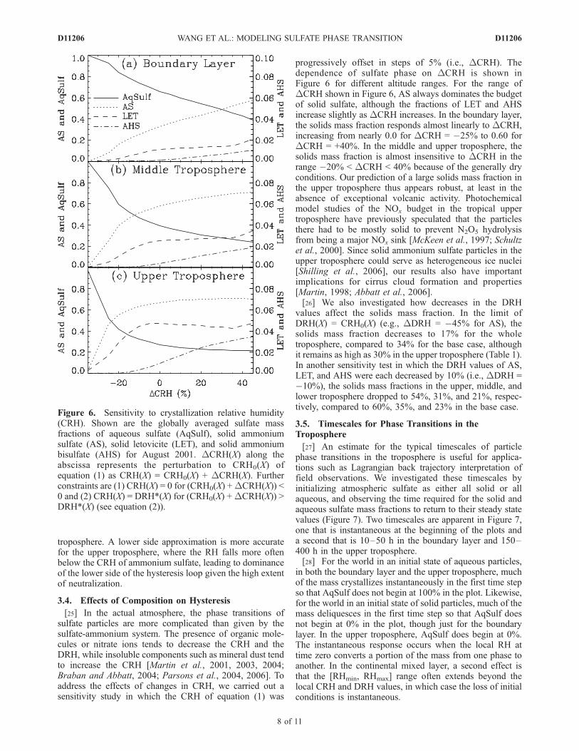
progressively offset in steps of 5% (i.e., DCRH). Thedependence of sulfate phase on DCRH is shown inFigure 6 for different altitude ranges. For the range ofDCRH shown in Figure 6, AS always dominates the budgetof solid sulfate, although the fractions of LET and AHSincrease slightly as DCRH increases. In the boundary layer,the solids mass fraction responds almost linearly to DCRH,increasing from nearly 0.0 for DCRH = �25% to 0.60 forDCRH = +40%. In the middle and upper troposphere, thesolids mass fraction is almost insensitive to DCRH in therange �20% < DCRH < 40% because of the generally dryconditions. Our prediction of a large solids mass fraction inthe upper troposphere thus appears robust, at least in theabsence of exceptional volcanic activity. Photochemicalmodel studies of the NOx budget in the tropical uppertroposphere have previously speculated that the particlesthere had to be mostly solid to prevent N2O5 hydrolysisfrom being a major NOx sink [McKeen et al., 1997; Schultzet al., 2000]. Since solid ammonium sulfate particles in theupper troposphere could serve as heterogeneous ice nuclei[Shilling et al., 2006], our results also have importantimplications for cirrus cloud formation and properties[Martin, 1998; Abbatt et al., 2006].[26] We also investigated how decreases in the DRH

values affect the solids mass fraction. In the limit ofDRH(X) = CRH0(X) (e.g., DDRH = �45% for AS), thesolids mass fraction decreases to 17% for the wholetroposphere, compared to 34% for the base case, althoughit remains as high as 30% in the upper troposphere (Table 1).In another sensitivity test in which the DRH values of AS,LET, and AHS were each decreased by 10% (i.e., DDRH =�10%), the solids mass fractions in the upper, middle, andlower troposphere dropped to 54%, 31%, and 21%, respec-tively, compared to 60%, 35%, and 23% in the base case.

3.5. Timescales for Phase Transitions in theTroposphere

[27] An estimate for the typical timescales of particlephase transitions in the troposphere is useful for applica-tions such as Lagrangian back trajectory interpretation offield observations. We investigated these timescales byinitializing atmospheric sulfate as either all solid or allaqueous, and observing the time required for the solid andaqueous sulfate mass fractions to return to their steady statevalues (Figure 7). Two timescales are apparent in Figure 7,one that is instantaneous at the beginning of the plots anda second that is 10–50 h in the boundary layer and 150–400 h in the upper troposphere.[28] For the world in an initial state of aqueous particles,

in both the boundary layer and the upper troposphere, muchof the mass crystallizes instantaneously in the first time stepso that AqSulf does not begin at 100% in the plot. Likewise,for the world in an initial state of solid particles, much of themass deliquesces in the first time step so that AqSulf doesnot begin at 0% in the plot, though just for the boundarylayer. In the upper troposphere, AqSulf does begin at 0%.The instantaneous response occurs when the local RH attime zero converts a portion of the mass from one phase toanother. In the continental mixed layer, a second effect isthat the [RHmin, RHmax] range often extends beyond thelocal CRH and DRH values, in which case the loss of initialconditions is instantaneous.

Figure 6. Sensitivity to crystallization relative humidity(CRH). Shown are the globally averaged sulfate massfractions of aqueous sulfate (AqSulf), solid ammoniumsulfate (AS), solid letovicite (LET), and solid ammoniumbisulfate (AHS) for August 2001. DCRH(X) along theabscissa represents the perturbation to CRH0(X) ofequation (1) as CRH(X) = CRH0(X) + DCRH(X). Furtherconstraints are (1) CRH(X) = 0 for (CRH0(X) +DCRH(X)) <0 and (2) CRH(X) = DRH*(X) for (CRH0(X) +DCRH(X)) >DRH*(X) (see equation (2)).


8 of 11

D11206

[29] After the instantaneous response, the solid and aque-ous sulfate mass fractions return to their steady state values,doing so more quickly in the boundary layer than in theupper troposphere. These timescales in large part reflect thevariability in RH in the different regions of the atmosphere.The boundary layer has both rapid mixing and large RHvertical gradients. The variability of RH in the uppertroposphere is much less, and the RH often lies in metasta-ble regions of CRH < RH < DRH.

4. Conclusions

[30] A simulation of the solid-aqueous phase transitionsof non-sea-salt sulfate-ammonium particles has been imple-mented in the GEOS-Chem global 3-D chemical transportmodel. The simulation explicitly includes consideration ofthe metastable behavior of aqueous sulfate particles in theCRH < RH < DRH range. Though with the minor simpli-fication that the initial and final deliquescence RH of mixedcomposition particles are equal, the hysteresis effect istreated by transporting aqueous and three solid sulfatephases in the CTM to retain the impact of RH history onsulfate phase and then diagnosing the phase changes every30 min on the basis of local relative humidity.

[31] We find that the solids mass fraction on a sulfatebasis is 0.34. Ammonium sulfate constitutes 93% of thesolid sulfate mass, with the balance from letovicite (6%) andammonium bisulfate (1%). A previous CTM simulation byColberg et al. [2003] found a solids mass fraction 5–10%smaller than ours and dominated by letovicite. The extent ofneutralization is greater in our simulation because of differ-ences in emission inventories and ammonia scavenging. Weaccount for the release of ammonia scavenged by clouddroplets upon droplet freezing, using a retention efficiencyof 0.05. Deep convection then injects ammonia into theupper troposphere. We thus find that sulfate particles in theupper troposphere are widely neutralized, consistent withthe few available observations. This has important implica-tions for atmospheric chemistry, specifically N2O5 hydro-lysis [McKeen et al., 1997], and also for cirrus cloudnucleation [Martin, 1998; Abbatt et al., 2006].[32] The solids mass fraction generally increases with

altitude, ranging from 22% in the boundary layer to 34% inmiddle troposphere to 60% in the upper troposphere. Thetimescale of phase transitions as driven by changes in RHvaries from 10 to 50 h in the boundary layer to 150–400 h inthe upper troposphere. The geographic distribution of solidsin the boundary layer is regulated more by the variation in

Figure 7. Temporal evolution of sulfate mass fractions of aqueous sulfate (AqSulf), solid ammoniumsulfate (AS), solid letovicite (LET), and solid ammonium bisulfate (AHS) from initial states of (left) allaqueous and (right) all solid. Results are shown for (top) the boundary layer and (bottom) the uppertroposphere for August 2001. (For the world in an initial state of solids, much of the mass deliquesces inthe first time step so that AqSulf does not begin at 0% in the plot. See text in section 3.5.)


9 of 11

D11206

RH than by particle neutralization. The opposite is the casein the upper troposphere.[33] The solids mass fraction peaks from May to October

in both hemispheres, largely reflecting emissions. The prin-cipal factor in the Northern Hemisphere is the summertimemaximum in NH3 biogenic emission. In the Southern Hemi-sphere, the principal factors are the winter minimum in DMSemission and the springtime maximum in NH3 emissionform biomass burning. Conversely, volcanic eruptions canlead to high acidity in the upper troposphere, as seen in oursimulation year for a Chilean volcano in March–April.[34] Omission of the hysteresis effect in global models by

assuming that particle phase follows the lower side of thehysteresis loop increases the solids mass fraction from 0.34to 0.56. An upper side assumption decreases the fraction to0.17. Lower and upper side assumptions better approximateparticle phase for high and low altitudes, respectively.[35] The CRH of metastable sulfate particles is sensitive

to other particle components besides ammonia, and weevaluated how shifting the CRH down (due to internalmixing with species such as organic molecules or nitrate)or up (due to mixing with heterogeneous nuclei such asmineral dust) affects phase partitioning. The solids massfraction is highly sensitive to DCRH in the boundary layerbut is almost independent of DCRH in the upper tropo-sphere for the range �20% < DCRH < +40%. Our findingof a large percentage of sulfate solids in the upper tropo-sphere should thus be insensitive to details in the sulfateparticle composition, although the model results must yet bevalidated by in situ observations of sulfate phase. Our workcorroborates past speculation that the upper troposphericsulfate mostly is in the solid phase, with implications forheterogeneous chemistry and cirrus cloud nucleation[Schultz et al., 2000; Abbatt et al., 2006].

[36] Acknowledgments. This research was supported by the NationalScience Foundation (Martin, grant ATM-0317583) and the NASA Atmo-spheric Composition Modeling and Analysis Program (Jacob). J. Wang wassupported by the NOAA Climate and Global Change postdoctoral fellow-ship program under the administration of the Visiting Scientist Program inUCAR.

ReferencesAbbatt, J. P. D., S. Benz, D. J. Cziczo, Z. Kanji, U. Lohmann, and O. Mohler(2006), Solid ammonium sulfate aerosols as ice nuclei: A pathway forcirrus cloud formation, Science, 313, 1770 – 1773, doi:10.1126/science.1129726.

Adams, P. J., J. H. Seinfeld, and D. M. Koch (1999), Global concentrationsof tropospheric sulfate, nitrate, and ammonium aerosol simulated in ageneral circulation model, J. Geophys. Res., 104, 13,791 –13,823,doi:10.1029/1999JD900083.

Adams, P. J., J. H. Seinfeld, D. Koch, L. Mickley, and D. Jacob (2001),General circulation model assessment of direct radiative forcing by thesulfate-nitrate-ammonium-water inorganic aerosol system, J. Geophys.Res., 106, 1097–1111, doi:10.1029/2000JD900512.

Allen, D. J., R. B. Rood, A. M. Thompson, and R. D. Hidson (1996),Three-dimension 222Rn calculations using assimilated data and a convec-tive mixing algorithm, J. Geophys. Res., 101, 6871–6881, doi:10.1029/95JD03408.

Andres, R. J., and A. D. Kasgnoc (1998), A time-averaged inventory ofsubaerial volcanic sulfur emissions, J. Geophys. Res., 103, 25,251–25,261, doi:10.1029/98JD02091.

Benkovitz, C. M., M. T. Scholtz, J. Pacyna, L. Tarrason, J. Dignon, E. C.Voldner, P. A. Spiro, J. A. Logan, and T. E. Graedel (1996), Globalgridded inventories of anthropogenic emissions of sulfur and nitrogen,J. Geophys. Res., 101, 29,239–29,253, doi:10.1029/96JD00126.

Bey, I., D. J. Jacob, R. M. Yantosca, J. A. Logan, B. Field, A. M. Fiore, Q. Li,H. Liu, L. J. Mickley, and M. Schultz (2001), Global modeling of tropo-spheric chemistry with assimilated meteorology: Model description and

evaluation, J. Geophys. Res., 106, 23,073 – 23,096, doi:10.1029/2001JD000807.

Biskos, G., A. Malinowski, L. M. Russell, P. R. Buseck, and S. T. Martin(2006a), Nanosize effect on the deliquescence and the efflorescence ofsodium chloride nanoparticles, Aerosol Sci. Technol., 40, 97 – 106,doi:10.1080/02786820500484396.

Biskos, G., D. Paulsen, L. M. Russell, P. R. Buseck, and S. T. Martin(2006b), Prompt deliquescence and efflorescence of aerosol nanoparti-cles, Atmos. Chem. Phys., 6, 4633–4642.

Bouwman, A. F., D. S. Lee, W. A. H. Asman, F. J. Dentener, K. W. Van DerHoek, and J. G. J. Olivier (1997), A global high-resolution emissioninventory for ammonia, Global Biogeochem. Cycles, 11, 561 –587,doi:10.1029/97GB02266.

Braban, C. F., and J. P. D. Abbatt (2004), A study of the phase transitionbehavior of internally mixed ammonium sulfate-malonic acid aerosols,Atmos. Chem. Phys., 4, 1451–1459.

Chin, M., and D. J. Jacob (1996), Anthropogenic and natural contributionsto tropospheric sulfate: A global model analysis, J. Geophys. Res., 101,18,691–18,699, doi:10.1029/96JD01222.

Clegg, S. L., P. Brimblecombe, and A. S. Wexler (1998), Thermodynamicmodel of the system H+-NH4

+-Na+-SO42��NO3

��Cl��H2O at 298.15 K,J. Phys. Chem. A, 102, 2155–2171, doi:10.1021/jp973043j.

Colberg, C. A., B. P. Luo, H. Wernli, T. Koop, and T. Peter (2003), A novelmodel to predict the physical state of atmospheric H2SO4/NH3/H2O aero-sol particles, Atmos. Chem. Phys., 3, 909–924.

Corbett, J. J., P. S. Fischbeck, and S. N. Pandis (1999), Global nitrogenand sulfur inventories for ocean-going ships, J. Geophys. Res., 104,3457–3470, doi:10.1029/1998JD100040.

Dibb, J. E., R. W. Talbot, and E. M. Scheuer (2000), Composition and dis-tribution of aerosols over the North Atlantic during the Subsonic Assess-ment Ozone and Nitrogen Oxide Experiment (SONEX), J. Geophys. Res.,105, 3709–3717, doi:10.1029/1999JD900424.

Dibb, J. E., R. W. Talbot, G. Seid, C. Jordan, E. Scheuer, E. Atlas, N. J.Blake, and D. R. Blake (2002), Airborne sampling of aerosol particles:Comparison between surface sampling at Christmas Island and P-3 sam-pling during PEM-Tropics B, J. Geophys. Res., 107, 8230, doi:10.1029/2001JD000408 [printed 108(D2), 2003].

Dibb, J. E., R. W. Talbot, E. M. Scheuer, G. Seid, M. A. Avery, and H. B.Singh (2003), Aerosol chemical composition in Asian continental out-flow during the TRACE-P campaign: Comparison with PEM-West B,J. Geophys. Res., 108(D21), 8815, doi:10.1029/2002JD003111.

Haywood, J., and O. Boucher (2000), Estimates of the direct and indirectradiative forcing due to tropospheric aerosols: A review, Rev. Geophys.,38, 513–543, doi:10.1029/1999RG000078.

Jaccard, C., and L. Levi (1961), Segregation d’impuretes dans la glace,Z. Agewandte Math. Phys., 12, 70–76, doi:10.1007/BF01601109.

Jacob, D. J. (2000), Heterogeneous chemistry and tropospheric ozone,Atmos. Environ., 34, 2131–2159, doi:10.1016/S1352-2310(99)00462-8.

Jacobson, M. Z. (2001), Global direct radiative forcing due to multicom-ponent anthropogenic and natural aerosols, J. Geophys. Res., 106, 1551–1568, doi:10.1029/2000JD900514.

Kane, S. M., F. Caloz, and M. T. Leu (2001), Heterogeneous uptake ofgaseous N2O5 by (NH4)2SO4, NH4HSO4, and H2SO4 aerosols, J. Phys.Chem. A, 105, 6465–6470, doi:10.1021/jp010490x.

Lehmann, C. M. B., V. C. Bowersox, R. S. Larson, and S. M. Larson(2007), Monitoring long-term trends in sulfate and ammonium in USprecipitation: Results from the National Atmospheric Deposition Pro-gram/National Trends Network, Water Air Soil Pollut., 7, 59 – 66,doi:10.1007/s11267-006-9100-z.

Lim, H. J., A. G. Carlton, and B. J. Turpin (2005), Isoprene forms sec-ondary organic aerosol through cloud processing: Model simulations,Environ. Sci. Technol., 39, 4441–4446, doi:10.1021/es048039h.

Lin, S.-J., and R. B. Rood (1996), Multidimensional flux from semi-Lagrangian transport scheme, Mon. Weather Rev., 124, 2046–2070,doi:10.1175/1520-0493(1996)124<2046:MFFSLT>2.0.CO;2.

Liu, H., et al. (2006), Radiative effect of clouds on tropospheric chemistryin a global three-dimensional chemical transport model, J. Geophys. Res.,111, D20303, doi:10.1029/2005JD006403.

Mari, C., D. J. Jacob, and P. Bechtold (2000), Transport and scavenging ofsoluble gases in a deep convective cloud, J. Geophys. Res., 105, 22,255–22,267, doi:10.1029/2000JD900211.

Martin, S. T. (1998), Phase transformations of the ternary system(NH4)2SO4-H2SO4-H2O and the implications for cirrus cloud formation,Geophys. Res. Lett., 25, 1657–1660, doi:10.1029/98GL00634.

Martin, S. T. (2000), Phase transitions of aqueous atmospheric particles,Chem. Rev., 100, 3403–3453, doi:10.1021/cr990034t.

Martin, S. T., J. H. Han, and H. M. Hung (2001), The size effect of hematiteand corundum inclusions on the efflorescence relative humidities of aqu-eous ammonium sulfate particles, Geophys. Res. Lett., 28, 2601–2604,doi:10.1029/2001GL013120.


10 of 11

D11206

Martin, S. T., J. C. Schlenker, A. Malinowski, H. M. Hung, and Y. Rudich(2003), Crystallization of atmospheric sulfate-nitrate-ammonium parti-cles, Geophys. Res. Lett., 30(21), 2102, doi:10.1029/2003GL017930.

Martin, S. T., H. M. Hung, R. J. Park, D. J. Jacob, R. J. D. Spurr, K. V.Chance, and M. Chin (2004), Effects of the physical state of troposphericammonium-sulfate-nitrate particles on global aerosol direct radiative for-cing, Atmos. Chem. Phys., 4, 183–214.

McKeen, S. A., T. Gierczak, J. B. Burkholder, P. O. Wennberg, T. F.Hanisco, E. R. Keim, R.-S. Gao, S. C. Liu, A. R. Ravishankara, andD. W. Fahey (1997), The photochemistry of acetone in the upper tropo-sphere: A source of odd-hydrogen radicals, Geophys. Res. Lett., 24,3177–3180, doi:10.1029/97GL03349.

Moorthi, S., and M. J. Suarez (1992), Relaxed Arakawa-Schubert. Aparameterizaiton of moist convection for general circulation models,Mon. Weather Rev., 120, 978 –1002, doi:10.1175/1520-0493(1992)120<0978:RASAPO>2.0.CO;2.

Park, R. J., D. J. Jacob, B. D. Field, R. M. Yantosca, and M. Chin (2004),Natural and transboundary pollution influences on sulfate-nitrate-ammonium aerosols in the United States: Implications for policy,J. Geophys. Res., 109, D15204, doi:10.1029/2003JD004473.

Parsons, M. T., D. A. Knopf, and A. K. Bertram (2004), Deliquescence andcrystallization of ammonium sulfate particles internally mixed withwater-soluble organic compounds, J. Phys. Chem. A, 108, 11,600–11,608, doi:10.1021/jp0462862.

Parsons, M. T., J. L. Riffell, and A. K. Bertram (2006), Crystallization ofaqueous inorganic-malonic acid particles: Nucleation rates, dependenceon size, and dependence on the ammonium-to-sulfate ratio, J. Phys.Chem. A, 110, 8108–8115, doi:10.1021/jp057074n.

Pruppacher, H. R., and J. D. Klett (2003), Microphysics of Clouds andPrecipitation, pp. 163–164, Springer, New York.

Ramaswamy, V., et al. (2001), Radiative forcing of climate change, inClimate Change 2001: The Scientific Basis—Contribution of WorkingGroup I to the Third Assessment Report of the Intergovernmental Panelon climate Change, edited by J. T. Houghton et al., pp. 349–416,Cambridge Univ. Press, New York.

Schlenker, J. C., and S. T. Martin (2005), Crystallization pathways ofsulfate-nitrate-ammonium aerosol particles, J. Phys. Chem. A, 109,9980–9985, doi:10.1021/jp052973x.

Schultz, M. G., D. J. Jacob, J. D. Bradshaw, S. T. Sandholm, J. E. Dibb,R. W. Talbot, and H. B. Singh (2000), Chemical NOx budget in the uppertroposphere over the tropical south Pacific, J. Geophys. Res., 105, 6669–6679, doi:10.1029/1999JD900994.

Seinfeld, J. H., and S. N. Pandis (1998), Atmospheric Chemistry andPhysics, John Wiley, New York.

Shilling, J. E., T. J. Fortin, and M. A. Tolbert (2006), Depositional icenucleation on crystalline organic and inorganic solids, J. Geophys.Res., 111, D12204, doi:10.1029/2005JD006664.

Spann, J. F., and C. B. Richardson (1985), Measurement of the water cyclein mixed ammonium acid sulfate particles, Atmos. Environ., 19, 819–825, doi:10.1016/0004-6981(85)90072-1.

Spiro, P. A., D. J. Jacob, and J. A. Logan (1992), Global inventory of sulfuremissions with 1� � 1� resolution, J. Geophys. Res., 97, 6023–6036.

Streets, D. G., et al. (2003), An inventory of gaseous and primary aerosolemissions in Asia in the year 2000, J. Geophys. Res., 108(D21), 8809,doi:10.1029/2002JD003093.

Talbot, R. W., J. E. Dibb, and M. B. Loomis (1998), Influence of verticaltransport on free tropospheric aerosols over the central USA in spring-time, Geophys. Res. Lett., 25, 1367–1370, doi:10.1029/98GL00184.

Tang, I. N., and H. R. Munkelwitz (1994), Aerosol phase-transformationand growth in the atmosphere, J. Appl. Meteorol., 33, 791 – 796,doi:10.1175/1520-0450(1994)033<0791:APTAGI>2.0.CO;2.

Wang, J., and S. T. Martin (2007), Satellite characterization of urban aero-sols: Importance of including hygroscopicity and mixing state in theretrieval algorithms, J. Geophys. Res., 112, D17203, doi:10.1029/2006JD008078.

Wang, J., D. J. Jacob, and S. T. Martin (2008), Sensitivity of sulfate directclimate forcing to the hysteresis of particle phase transitions, J. Geophys.Res., 113, D11207, doi:10.1029/2007JD009368.

��A. A. Hoffmann, D. J. Jacob, and S. T. Martin, School of Engineering

and Applied Sciences, Harvard University, Cambridge, MA 02138, USA.([email protected])R. J. Park, School of Earth and Environmental Sciences, Seoul National

University, San 56-1, Sillim, Gwanakgu, Seoul 151-742, South Korea.J. Wang, Department of Geosciences, University of Nebraska–Lincoln,

Lincoln, NE 68588, USA. ([email protected])


11 of 11

D11206

global distribution of solid and aqueous sulfate aerosols...

Documents