w.elsevier.com/locate/rse

Remote Sensing of Environmen

Global distribution of Case-1 waters: An analysis

from SeaWiFS measurements

ZhongPing Lee a,*, Chuanmin Hu b

a Naval Research Lab, Code 7333, Stennis Space Center, MS 39529, USAb College of Marine Science, University of South Florida, 140 Seventh Ave., South St. Petersburg, FL 33701, USA

Received 22 June 2005; received in revised form 7 October 2005; accepted 5 November 2005

Abstract

‘‘Case-1’’ has been a term frequently used to characterize water type since the seventies. However, the distribution of Case-1 waters in global

scale has been vague, though open ocean waters are often referred to as Case-1 in the literature. In this study, based on recent bio-optical models

for Case-1 waters, an inclusive and quantitative Case-1 criterion for remote sensing applications is developed. The criterion allows Case-1 waters

to have about two-fold variations of non-pigment absorption and particle backscattering around their exact Case-1 values, allowing a large range

of waters to be classified as Case-1. Even so, application of this criterion to ocean color data from the SeaWiFS satellite sensor suggests that Case-

1 waters occupy only about 60% of the global ocean surface. Regionally, more Case-1 waters are found in the southern hemisphere than in the

northern hemisphere, and most Indian Ocean waters are found to be Case-1. The Case-1 percentage and spatial distribution change with season,

and with the boundaries chosen in the criterion. Nevertheless, this study for the first time provides a quantitative and geographical perspective of

Case-1 waters in global scale, and further demonstrates that many open ocean waters are not necessarily Case-1.

D 2005 Elsevier Inc. All rights reserved.

Keywords: Case-1; Case-2; Ocean color; Remote sensing; Bio-optical model

1. Introduction

Studies of ocean optics in the past decades have found that

there are three major water constituents in addition to water

molecules that determine water’s inherent optical properties

(absorption and scattering): phytoplankton and its associates,

colored dissolved organic matter (CDOM), and inorganic

mineral particles (Carder et al., 1991; IOCCG, 2000; Sathyen-

dranath et al., 1989). In modeling the optical properties and in

particular to retrieve the phytoplankton pigment (chlorophyll-a)

concentration from ocean color (i.e., water-leaving radiance or

radiance of sea), a scheme to simplify the dependence of

optical properties on water constituents was proposed: i.e., the

Case-1 and Case-2 separation of natural waters (Morel, 1988;

Morel & Prieur, 1977).

The concept of Case-1 and Case-2 waters, originally

proposed by Morel and Prieur (1977), has evolved over the

past decades (Gordon & Morel, 1983; IOCCG, 2000; Mobley

0034-4257/$ - see front matter D 2005 Elsevier Inc. All rights reserved.

doi:10.1016/j.rse.2005.11.008

* Corresponding author.

E-mail address: zplee@nrlssc.navy.mil (ZP. Lee).

et al., 2004; Morel, 1988; Prieur & Sathyendranath, 1981; also

see Mobley et al., 2004 for review), and the definitions are not

uniform. Commonly, Case-1 waters are those whose inherent

optical properties (Preisendorfer, 1976) can be adequately

described by phytoplankton (represented by chlorophyll

concentration, or Chl) (Gordon & Morel, 1983; IOCCG,

2000; Morel, 1988), whereas Case-2 waters are otherwise. In

other words, Case-1 waters, at least, require that the optical

properties of other optically active constituents (CDOM and

particles in particular) closely follow the optical properties of

phytoplankton (Morel, 1988; Morel & Maritorena, 2001).

Clearly, this definition of Case-1 water is not based on its

geographical location, nor on the Chl value. In fact, coastal

waters could be Case-1, whereas open ocean waters could be

Case-2. However, the term ‘‘Case-1’’ is frequently used in the

literature to characterize open ocean waters.

On the other hand, in the recent decades, many bio-optical

models, remote-sensing algorithms for Chl retrievals, and

applications in ocean-color remote sensing have been developed

specifically for Case-1 waters e.g. (Gross et al., 2000; Haltrin,

1999; Morel, 1988; Morel & Maritorena, 2001; Ohlmann et al.,

t 101 (2006) 270 – 276

ww

Z. Lee, C. Hu / Remote Sensing of Environment 101 (2006) 270–276 271

2000; O’Reilly et al., 1998; Stamnes et al., 2003). For instance,

in the NASA software package SeaDAS, the default band-ratio

algorithm used to estimate Chl requires water to be Case-1

(SeaWiFS, 2000). To use these Case-1 specific models and

algorithms, knowledge of the distribution of Case-1 waters in

global scale and its temporal variations is required.

Ideally, concurrent measurements of both optical properties

(absorption and scattering) and Chl are required to map the

global distribution of Case-1 waters. In practice, however, the

only feasible means is to use ocean color data from satellite

sensors. Therefore, based on the latest bio-optical models for

Case-1 waters developed from extensive measurements (Morel

& Maritorena, 2001), in this study we devised an inclusive

remote-sensing criterion to map Case-1 waters using remote-

sensing reflectance (a measure of ocean color). Further, we

applied this criterion to the lately updated satellite data from

the Sea-viewing Wide Field-of-view Sensor (SeaWiFS,

‘‘reprocessing 4’’) to provide a global perspective of Case-1

waters and its seasonal variations for the first time. Our goal is

to obtain a quantitative understanding of the Case-1 water

distribution on a global scale. In particular, we want to

examine whether most open ocean waters (i.e., 90% or more)

are Case-1.

2. Remote-sensing criterion for Case-1 waters

After atmospheric correction, spectral water-leaving radi-

ance is derived from the radiance data collected by an ocean

color satellite sensor (Gordon, 1997). This radiance can be

easily converted to spectral remote-sensing reflectance (Rrs(k)),defined as a ratio of water-leaving radiance to downwelling

irradiance just above the surface. The latter can be adequately

modeled with information derived from the process of

atmospheric correction, for example, aerosol type and optical

thickness (Gordon, 1997).

Absorption, backscattering, and diffuse attenuation coeffi-

cients as well as Chl could be further derived from Rrs(k) witha bio-optical algorithm (e.g., Carder et al., 1999; Hoge & Lyon,

1996; Lee et al., 2002; Maritorena et al., 2000; Mueller &

Trees, 1997; Roesler & Perry, 1995). However, such derived

parameters are associated with various uncertainties, especially

for Chl, due to the assumptions used in the algorithms, such as

the spectral shapes of chlorophyll and CDOM absorption

(Nelson & Robertson, 1993; Wang et al., 2005), the specific-

absorption coefficient of Chl (Bricaud et al., 1995, 1981), and

so on. Different algorithms may yield different Chl estimates

(O’Reilly et al., 1998). These characteristics make it difficult to

use the derived parameters to map Case-1 waters. Causing

further uncertainty is that sometimes the water type (Case-1 or

Case-2) needs to be known before an algorithm is used to

derive these parameters (O’Reilly et al., 1998). Hence, it is

highly desirable to use Rrs(k) directly to separate water types

such as Case-1 and Case-2.

As previously noted, Case-1 definitions are not uniform in

the literature (Mobley et al., 2004). However, here we concur

with the generally accepted concept that Case-1 waters are

those whose inherent optical properties can be determined

solely by Chl (Gordon & Morel, 1983; Loisel & Morel, 1998;

Morel, 1988). Therefore, for optically deep waters, a unique

relationship exists between Chl and Case-1 Rrs(k) (Haltrin,

1999; Morel, 1988; Morel & Maritorena, 2001). And, based on

the Case-1 bio-optical models developed from extensive

measurements of Chl and optical properties, the spectral

remote-sensing reflectance (Rrs(k)) of Case-1 waters can be

calculated when Chl is known (Maritorena & Siegel, 2005;

Morel & Maritorena, 2001). Specifically, spectral models have

been developed to calculate Case-1 water diffuse attenuation

(Kd) and backscattering (bb) coefficients for a given chloro-

phyll value (Loisel & Morel, 1998; Morel, 1988; Morel &

Maritorena, 2001). In the initial steps of calculating absorption

coefficient (a) and irradiance reflectance (R) (Morel &

Maritorena, 2001), Kd is converted to absorption coefficient

with an average cosine (Kirk, 1994) value of 0.75, and R is

¨0.33bb/a. This R value is then combined with Kd to calculate

another set of a following the Gershun’s equation (Morel &

Maritorena, 2001). After three iterations (Morel & Maritorena,

2001), stable a(k) and R(k) values are obtained. Because Rrs is

also a function of bb/a for Case-1 waters (Morel & Gentili,

1993), Rrs(k) is obtained for the given Chl. Following this

approach, Case-1 Rrs(k) were calculated for Chl values ranging

between 0.02 and 30.0 mg m�3 (500 points with a step of

¨0.01 in log scale). Further, the following spectral ratios were

derived:

RR12 ¼Rrs 412ð ÞRrs 443ð Þ ; RR53 ¼

Rrs 555ð ÞRrs 490ð Þ : ð1Þ

Here 412, 443, 490, and 555 are the center wavelengths (in nm)

of SeaWiFS bands 1, 2, 3, and 5, respectively. RR12 represents

the relative abundance of CDOM per Chl (Carder et al., 1999),

RR53 is viewed as a measure of Chl (e.g., Aiken et al., 1995;

O’Reilly et al., 1998) and Rrs(555) as a measure of particle

backscattering (Carder et al., 1999).

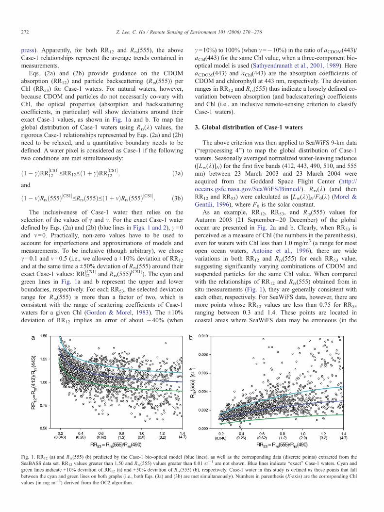
A monotonic line exists between the calculated RR12 and

RR53 values (the blue line in Fig. 1a), because by definition

optical properties of Case-1 waters are determined by Chl

alone. This monotonic line can be represented accurately (less

than 1% error) by the following empirical polynomial function

(RR53 in a range of ¨0.2 to ¨2.0):

RRCS1½ �12 ¼ 0:9351þ 0:113=RR53 � 0:0217= RR53ð Þ2

þ 0:003= RR53ð Þ3: ð2aÞ

The superscript [CS1] represents Case-1. Similarly, a mono-

tonic line exists between Rrs(555) and RR53 for Case-1 waters

(blue line in Fig. 1b):

Rrs 555ð Þ CS1½ � ¼ 0:0006þ 0:0027 RR53 � 0:0004 RR53ð Þ2

� 0:0002 RR53ð Þ3: ð2bÞ

Included in Fig. 1a and b are the dependences of RR12 and

Rrs(555) on RR53 (discrete points), calculated from field-

measured Rrs data extracted from the SeaWiFS Bio-optical

Archive and Storage System (SeaBASS, Werdell & Bailey, in

Z. Lee, C. Hu / Remote Sensing of Environment 101 (2006) 270–276272

press). Apparently, for both RR12 and Rrs(555), the above

Case-1 relationships represent the average trends contained in

measurements.

Eqs. (2a) and (2b) provide guidance on the CDOM

absorption (RR12) and particle backscattering (Rrs(555)) per

Chl (RR53) for Case-1 waters. For natural waters, however,

because CDOM and particles do not necessarily co-vary with

Chl, the optical properties (absorption and backscattering

coefficients, in particular) will show deviations around their

exact Case-1 values, as shown in Fig. 1a and b. To map the

global distribution of Case-1 waters using Rrs(k) values, the

rigorous Case-1 relationships represented by Eqs. (2a) and (2b)

need to be relaxed, and a quantitative boundary needs to be

defined. A water pixel is considered as Case-1 if the following

two conditions are met simultaneously:

1� cð ÞRR CS1½ �12 VRR12V 1þ cð ÞRR CS1½ �

12 ; ð3aÞ

and

1� mð ÞRrs 555ð Þ CS1½ �VRrs 555ð ÞV 1þ mð ÞRrs 555ð Þ CS1½ �: ð3bÞ

The inclusiveness of Case-1 water then relies on the

selection of the values of c and m. For the exact Case-1 water

defined by Eqs. (2a) and (2b) (blue lines in Figs. 1 and 2), c =0and m =0. Practically, non-zero values have to be used to

account for imperfections and approximations of models and

measurements. To be inclusive (though arbitrary), we chose

c =0.1 and m=0.5 (i.e., we allowed a T10% deviation of RR12

and at the same time a T50% deviation of Rrs(555) around their

exact Case-1 values: RR[CS1]12 and Rrs(555)

[CS1]). The cyan and

green lines in Fig. 1a and b represent the upper and lower

boundaries, respectively. For each RR53, the selected deviation

range for Rrs(555) is more than a factor of two, which is

consistent with the range of scattering coefficients of Case-1

waters for a given Chl (Gordon & Morel, 1983). The T10%deviation of RR12 implies an error of about �40% (when

Fig. 1. RR12 (a) and Rrs(555) (b) predicted by the Case-1 bio-optical model (blue

SeaBASS data set. RR12 values greater than 1.50 and Rrs(555) values greater than

green lines indicate T10% deviation of RR12 (a) and T50% deviation of Rrs(555)

between the cyan and green lines on both graphs (i.e., both Eqs. (3a) and (3b) are m

values (in mg m�3) derived from the OC2 algorithm.

c =10%) to 100% (when c=�10%) in the ratio of aCDOM(443)/

aChl(443) for the same Chl value, when a three-component bio-

optical model is used (Sathyendranath et al., 2001, 1989). Here

aCDOM(443) and aChl(443) are the absorption coefficients of

CDOM and chlorophyll at 443 nm, respectively. The deviation

ranges in RR12 and Rrs(555) thus indicate a loosely defined co-

variation between absorption (and backscattering) coefficients

and Chl (i.e., an inclusive remote-sensing criterion to classify

Case-1 waters).

3. Global distribution of Case-1 waters

The above criterion was then applied to SeaWiFS 9-km data

(‘‘reprocessing 4’’) to map the global distribution of Case-1

waters. Seasonally averaged normalized water-leaving radiance

([Lw(k)]N) for the first five bands (412, 443, 490, 510, and 555

nm) between 23 March 2003 and 23 March 2004 were

acquired from the Goddard Space Flight Center (http://

oceans.gsfc.nasa.gov/SeaWiFS/Binned/). R rs(k) (and then

RR12 and RR53) were calculated as [Lw(k)]N/F0(k) (Morel &

Gentili, 1996), where F0 is the solar constant.

As an example, RR12, RR53, and Rrs(555) values for

Autumn 2003 (21 September–20 December) of the global

ocean are presented in Fig. 2a and b. Clearly, when RR53 is

perceived as a measure of Chl (the numbers in the parenthesis),

even for waters with Chl less than 1.0 mg/m3 (a range for most

open ocean waters, Antoine et al., 1996), there are wide

variations in both RR12 and Rrs(555) for each RR53 value,

suggesting significantly varying combinations of CDOM and

suspended particles for the same Chl value. When compared

with the relationships of RR12 and Rrs(555) obtained from in

situ measurements (Fig. 1), they are generally consistent with

each other, respectively. For SeaWiFS data, however, there are

more points whose RR12 values are less than 0.75 for RR53

ranging between 0.3 and 1.4. These points are located in

coastal areas where SeaWiFS data may be erroneous (in the

lines), as well as the corresponding data (discrete points) extracted from the

0.01 sr�1 are not shown. Blue lines indicate ‘‘exact’’ Case-1 waters. Cyan and

(b), respectively. Case-1 water in this study is defined as those points that fall

et simultaneously). Numbers in parenthesis (X-axis) are the corresponding Chl

Fig. 2. Similar to Fig. 1, but the discrete data points represent those extracted from the SeaWiFS global data for Autumn 2003 (21 Sept.–20 Dec. 2003). RR12 values

less than 0.50 and Rrs(555) values greater than 0.01 sr�1 are not shown.

Z. Lee, C. Hu / Remote Sensing of Environment 101 (2006) 270–276 273

blue bands, in particular) due to the imperfect atmospheric

correction (e.g., Hu et al., 2000). Another possible reason is

that the field data from SeaBASS did not cover the global

ocean evenly. Nevertheless, these points contribute about 5%

of the SeaWiFS observed sea surface, therefore have limited

effects to the analyses of global distribution of Case-1 waters.

Fig. 3 shows the global distribution of Case-1 and non-Case-

1 waters based on the inclusive remote-sensing criterion (Eqs.

(3a) and (3b)). Approximately 60% of the global surface water

is found to belong to the Case-1 category. Regionally, most of

the Case-1 waters are in the tropical and subtropical areas, along

with waters in the Indian Ocean. About half of the non-Case-1

waters are found in high latitudes (especially in the northern

hemisphere), and many of them are open ocean waters. In the

63% Case-1

Spring

Autumn

66% Case-1

Fig. 3. Global distribution of Case-1 waters (blue color) and its seasonal variatio

mid Pacific, a lot of surface waters (these waters do not

necessarily overlap with the equatorial upwelling regions) do

not meet the Case-1 criterion, possibly due to lower CDOM per

Chl (see below, and Siegel et al., 2005) than those predicted by

the Case-1 bio-optical model (Morel & Maritorena, 2001).

Seasonally, there is no substantial change in the total percentage

of Case-1 waters from Spring to Autumn, but the percentage

drops significantly in Winter, a result from a significant increase

of non-Case-1 waters in the southern high latitudes. The spatial

distribution of Case-1 waters also varies seasonally.

To examine the individual effects of the two conditions set

by Eqs. (3a) and (3b), Fig. 4a and b exemplify Case-1 water

distribution when only one of the conditions is applied,

respectively. In Fig. 4a, where Eq. (3a) alone was applied,

Summer

Winter

63% Case-1

56% Case-1

ns as derived from SeaWiFS measurements. See text for Case-1 definition.

Fig. 4. SeaWiFS-derived Case-1 waters (blue color) for Autumn 2003 defined by Eq. (3a) with c =0.1 (a) and by Eq. (3b) with m =0.5 (b), respectively. In (a), cyan

color represents RR12>1.1RR[CS1]12 ; green color represents RR12 between 0.5 and 0.9RR[CS1]

12 ; and red color for RR12<0.5. In (b), cyan color represents

Rrs(555)>1.5Rrs(555)[CS1]; and green color for Rrs(555)<0.5Rrs(555)

[CS1].

Z. Lee, C. Hu / Remote Sensing of Environment 101 (2006) 270–276274

¨76% of the global surface ocean (blue color) belongs to this

further relaxed Case-1 category. For a large portion of waters in

the mid Pacific (cyan color), their RR12 values are greater than

1.1RR[CS1]12 , indicating relatively lower CDOM per Chl (Siegel

et al., 2005). In the high latitude northern hemisphere (green

color), RR12 value are smaller than 0.9RR[CS1]12 and indicate

relatively higher CDOM per Chl. This is because Rrs is

inversely proportional to absorption coefficient (Morel &

Gentili, 1993), smaller RR12 values indicate higher absorption

by CDOM at 412 nm (and then relatively more CDOM) (Carder

et al., 1999; Sathyendranath et al., 2001; Siegel et al., 2005).

Note that CDOM absorption also affects the spectral ratio of

Rrs(k) (Carder et al., 1989; Sathyendranath et al., 2001).

Therefore, if the same empirical band-ratio Chl algorithm

(e.g., OC2 or OC4 algorithm, O’Reilly et al., 1998) is applied to

the global ocean, Chl may be overestimated in the green colored

waters while underestimated in the cyan colored waters, even

without considering the phytoplankton ‘‘packaging effect’’

(Bricaud et al., 1995; Bricaud & Morel, 1986).

Fig. 4b shows the distribution of Case-1 waters during

Autumn 2003 when Eq. (3b) alone was applied (m =0.5). Thepercentage of such Case-1 waters in the global ocean is ¨88%,

a result of the relatively large m value. Most (¨90%) of the

cyan colored waters, representing higher backscattering per

Chl, are in the high latitude southern hemisphere, with the rest

spread around many coastal regions (especially river plumes).

Clearly, the effects of the two criteria do not completely

overlap, suggesting independent variations of absorption and

Fig. 5. Global distribution of Case-1 waters (blue color) for Autumn 2003 when

the criterion for Case-1 definition is slightly tightened, i.e., m in Eq. (3b) is

changed from 0.5 to 0.3 while c in Eq. (3a) remains as 0.1.

scattering coefficients, which might be the results of different

biogeochemical processes (e.g., Balch et al., 2005; Behrenfeld

et al., 2005; Boss & Zaneveld, 2003).

The percentage of Case-1 waters depends on the quantita-

tive boundaries (c and m values). For example in Fig. 5, where

we keep c =0.1 but change m from 0.5 to 0.3 (which still

represents a factor of 1.8 deviation range in Rrs(555)), we see

the effects of more tightly defined Case-1 waters for Autumn

2003, where the percentage of Case-1 waters (blue color) drops

to 32%. Even so, using this slightly tightened standard, some

coastal waters may still belong to Case-1, while many open

ocean waters fall out of the Case-1 category. Indeed, the optical

properties of many open ocean waters do not co-vary with Chl

(Siegel & Michaels, 1996), if the quantitative standard for ‘‘co-

vary’’ is a T30% deviation range from its expected value.

4. Summary

In this study, an inclusive Case-1 remote-sensing criterion

was developed from the widely accepted Case-1 bio-optical

models (Morel & Maritorena, 2001). This criterion compares

the relationships between Rrs(412)/Rrs(443) and Rrs(555)/

Rrs(490), and between Rrs(555) and Rrs(555)/Rrs(490), to their

expected Case-1 values from the bio-optical models. Because

only limited natural waters follow the quantitative relationships

for Case-1 waters exactly, some boundaries were selected to

include more waters as Case-1 (Gordon & Morel, 1983). The

boundaries include a T10% deviation in Rrs(412)/Rrs(443) and

a T50% deviation in Rrs(555) from their exact Case-1 values.

Such boundaries are corresponding to about two-fold variations

in the aCDOM(443)/aChl(443) ratio and in the backscattering

coefficient at 555 nm for the same Chl value, respectively.

Application of this inclusive Case-1 remote-sensing criteri-

on to the lately updated (‘‘reprocessing 4’’), seasonally

averaged (less random errors than daily collections), SeaWiFS

data yielded global distribution of Case-1 waters. Only about

60% of global surface waters could be considered as Case-1 by

this criterion. A substantial portion of the open ocean is non-

Case-1. The spatial distribution of Case-1 waters changes with

season. Further, Case-1 distribution patterns obtained from the

two individual conditions (absorption component and scatter-

ing component) do not always overlap, suggesting indepen-

dently varying water constituents. The spatial resolution of the

SeaWiFS data used in this study is 9 km, as used in other

Z. Lee, C. Hu / Remote Sensing of Environment 101 (2006) 270–276 275

global studies (e.g., Siegel et al., 2005). Because oceanic

waters are relatively uniform over large distances, we would

not expect our results to change significantly if higher spatial

resolution data were used.

The Case-1 coverage, as shown above, strongly depends on

the deviation boundaries chosen in the criterion. For example,

if the T50% deviation for Rrs(555) is tightened to T30%, the

global Case-1 percentage drops to ¨32% for measurements

made in Autumn 2003. The Case-1 distribution also depends

on the quality of the Rrs data from the satellite sensor. Though

Rrs of open ocean is believed to be accurately retrieved from

the SeaWiFS sensor (Gordon & Wang, 1994), it is well known

that it is troublesome to accurately remove the atmospheric

effects in coastal regions. However, because coastal waters

only occupy a small portion of the global ocean surface (e.g.,

only ¨5% of the water pixels are associated with RR12 values

less than 0.75), the effects of erroneous coastal Rrs on the

global Case-1 water distribution are expected to be small.

From the results presented here and from earlier discrete

measurements (Bricaud et al., 1981), it is clear that many open

ocean waters are not necessarily Case-1, while coastal and

highly productive waters can be Case-1. Indeed, even in the

clearest open ocean waters, the Sargasso Sea, water constituents

have been found to not co-vary (Siegel & Michaels, 1996) or

co-vary but with a time lag or phase shift (Hu et al., in press).

There is no doubt that the Case-1 bio-optical models (Morel,

1988; Morel & Maritorena, 2001) provide us an easy and

useful tool to quickly estimate water’s optical properties simply

by concentrations of chlorophyll. It is necessary to keep in

mind, however, that there are large deviations around the

statistically averaged values even for open ocean waters. As

pointed out by Morel and Prieur (1977) in their seminal paper,

there is often no clear optical or geographical boundary

between Case-1 and Case-2 waters. Hence, the Case-1

percentage as well as its spatial coverage presented in this

study should not be treated in an absolute sense. Rather, they

serve synoptically as a cautious note to algorithm developers

and oceanographers when the term ‘‘Case-1’’ is used. For more

reliable applications of remote sensing algorithms, it is better to

take approaches or algorithms that do not need a Case-1 clause,

as suggested by Mobley et al. (2004). Further, now with the

improved ability to derive global distributions of aChl, aCDOM,

and particle backscattering from satellite data (Carder et al.,

1999; Doerffer & Schiller, 2006; Hoge & Lyon, 1996; Lee et

al., 2002; Loisel & Stramski, 2000; Maritorena et al., 2000), it

would be much more useful to define and map water masses

based explicitly on these optical properties (Behrenfeld et al.,

2005; Gould & Arnone, 2003; Prieur & Sathyendranath, 1981)

that directly control the radiance of sea.

Acknowledgements

Financial support was provided by an ONR (Environmental

Optics Program) grant N0001405WX20623 (Lee) and by a

NASA grant NAG5-10738 (Hu). We thank Sean Bailey

(NASA) and Sherwin Ladner (PSI) for their assistance in

SeaWiFS data acquisition, and the four anonymous reviewers

for their constructive comments and suggestions. IMaRS

contribution #101.

References

Aiken, J., Moore, G. F., Trees, C. C., Hooker, S. B., & Clark, D. K. (1995). The

SeaWiFS CZCS-type pigment algorithm. In S. B. Hooker, & E. R. Firestone

(Eds.), NASA technical memorandum, 104566. SeaWiFS technical report

series, vol. 29 (pp. 1–32).

Antoine, D., Andre, J.-M., & Morel, A. (1996). Oceanic primary production 2.

Estimation at global scale from satellite (coastal zone color scanner)

chlorophyll. Global Biogeochemical Cycles, 10(1), 57–69.

Balch, W. M., Gordon, H. R., Bowler, B. C., Drapeau, D. T., & Booth, E. S.

(2005). Calcium carbonate measurements in the surface global ocean based

on Moderate-Resolution Imaging Spectroradiometer data. Journal of

Geophysical Research, 110(C07001). doi:10.1029/2004JC002560.

Behrenfeld, M. J., Boss, E., Siegel, D., & Shea, D. M. (2005). Carbon-based

ocean productivity and phytoplankton physiology from space. Global

Biogeochemical Cycles, 19, GB1006. doi:10.1029/2004GB002299.

Boss, E., & Zaneveld, J. R. V. (2003). The effect of bottom substrate on

inherent optical properties: Evidence of biogeochemical processes. Limnol-

ogy and Oceanography, 48, 346–354.

Bricaud, A., Babin, M., Morel, A., & Claustre, H. (1995). Variability in the

chlorophyll-specific absorption coefficients of natural phytoplankton:

Analysis and parameterization. Journal of Geophysical Research, 100,

13321–13332.

Bricaud, A., & Morel, A. (1986). Light attenuation and scattering

by phytoplanktonic cells: A theoretical modeling. Applied Optics, 25,

571–580.

Bricaud, A., Morel, A., & Prieur, L. (1981). Absorption by dissolved organic

matter of the sea (yellow substance) in the UV and visible domains.

Limnology and Oceanography, 26, 43–53.

Carder, K. L., Chen, F. R., Lee, Z. P., Hawes, S. K., & Kamykowski, D. (1999).

Semianalytic Moderate-Resolution Imaging Spectrometer algorithms

for chlorophyll-a and absorption with bio-optical domains based on

nitrate-depletion temperatures. Journal of Geophysical Research, 104,

5403–5421.

Carder, K. L., et al. (1991). Reflectance model for quantifying chlorophyll a in

the presence of productivity degradation products. Journal of Geophysical

Research, 96, 20599–20611.

Carder, K. L., Steward, R. G., Harvey, G. R., & Ortner, P. B. (1989). Marine

humic and fulvic acids: Their effects on remote sensing of ocean

chlorophyll. Limnology and Oceanography, 34, 68–81.

Doerffer, R. & Schiller, H. (in press). The MERIS case 2 water algorithm.

International Journal of Remote Sensing.

Gordon, H. R. (1997). Atmospheric correction of ocean color imagery in the

Earth observing system era. Journal of Geophysical Research, 102(D),

17081–17106.

Gordon, H. R., & Morel, A. (1983). Remote assessment of ocean color

for interpretation of satellite visible imagery: A review. New York’

Springer-Verlag.

Gordon, H. R., & Wang, M. (1994). Retrieval of water-leaving radiance and

aerosol optical thickness over oceans with SeaWiFS: A preliminary

algorithm. Applied Optics, 33, 443–452.

Gould, R. W. & Arnone, R. A. (2003). Optical Water Mass Classification for

Ocean Color Imagery, Second International Conference, Current Problems

in Optics Of Natural Waters, St. Petersburg, Russia.

Gross, L., Thiria, S., Frouin, R., & Mitchell, B. G. (2000). Artificial neural

networks for modeling the transfer function between marine reflectance and

phytoplankton pigment concentration. Journal of Geophysical Research,

105(C2), 3483–3496.

Haltrin, V. I. (1999). Chlorophyll-based model of seawater optical properties.

Applied Optics, 38(33), 6826–6832.

Hoge, F. E., & Lyon, P. E. (1996). Satellite retrieval of inherent optical

properties by linear matrix inversion of oceanic radiance models: An

analysis of model and radiance measurement errors. Journal of Geophysical

Research, 101, 16631–16648.

Z. Lee, C. Hu / Remote Sensing of Environment 101 (2006) 270–276276

Hu, C., Carder, K. L., & Mueller-Karger, F. E. (2000). Atmospheric correction

of SeaWiFS imagery over turbid coastal waters: A practical method.

Remote Sensing of Environment, 74, 195–206.

Hu, C., Lee, Z. P., Muller-Karger, F. E., Carder, K. L., & Walsh, J. J. (in press).

Ocean color reveals phase shift between marine plants and yellow

substance. IEEE Geoscience and Remote Sensing Letters.

IOCCG (2000). Remote sensing of ocean colour in coastal, and other optically-

complex, waters. In S. Sathyendranath (Ed.), Reports of the International

Ocean-Colour Coordinating Group, No.3. Dartmouth, Canada’ IOCCG.

Kirk, J. T. O. (1994). Light and photosynthesis in aquatic ecosystems.

Cambridge’ University Press.

Lee, Z. P., Carder, K. L., & Arnone, R. (2002). Deriving inherent optical

properties from water color: A multi-band quasi-analytical algorithm for

optically deep waters. Applied Optics, 41, 5755–5772.

Loisel, H., & Morel, A. (1998). Light scattering and chlorophyll concentration

in Case 1 waters: A reexamination. Limnology and Oceanography, 43,

847–858.

Loisel, H., & Stramski, D. (2000). Estimation of the inherent optical properties

of natural waters from the irradiance attenuation coefficient and reflectance

in the presence of Raman scattering. Applied Optics, 39, 3001–3011.

Maritorena, S., & Siegel, D. A. (2005). Consistent merging of satellite ocean

color data sets using a bio-optical model. Remote Sensing of Environment,

94, 429–440.

Maritorena, S., Siegel, D. A., & Peterson, A. R. (2000). Optimization of a

semianalytical ocean color model for global-scale applications. Applied

Optics, 41, 2705–2714.

Mobley, C. D., Stramski, D., Bissett, W. P., & Boss, E. (2004). Optical

modeling of ocean waters: Is the Case 1–Case 2 classification still useful?

Oceanography, 17(2), 60–67.

Morel, A. (1988). Optical modeling of the upper ocean in relation to its

biogenous matter content (Case I waters). Journal of Geophysical Research,

93, 10749–10768.

Morel, A., & Gentili, B. (1993). Diffuse reflectance of oceanic waters (2): Bi-

directional aspects. Applied Optics, 32, 6864–6879.

Morel, A., & Gentili, B. (1996). Diffuse reflectance of oceanic waters: III.

Implications of bi-directionality for the remote sensing problem. Applied

Optics, 35, 4850–4862.

Morel, A., & Maritorena, S. (2001). Bio-optical properties of oceanic waters: A

reappraisal. Journal of Geophysical Research, 106, 7163–7180.

Morel, A., & Prieur, L. (1977). Analysis of variations in ocean color. Limnology

and Oceanography, 22, 709–722.

Mueller, J. L., & Trees, C. C. (Eds.) (1997). Revised Sea WIFS prelaunch

algorithm for diffuse attenuation coefficient K(490). Case Studies for

SeaWiFS Calibration and Validation, NASA Tech Memo. 104566, 41.

Greenbelt, MD’ NASA Goddard Space Flight Center.

Nelson, J. R., & Robertson, C. Y. (1993). Detrital spectral absorption:

Laboratory studies of visible light effects on phytodetritus absorption,

bacterial spectral signal, and comparison to field measurements. Journal of

Marine Research, 51, 181–207.

Ohlmann, J. C., Siegel, D. A., & Mobley, C. D. (2000). Ocean radiant

heating: Part I. Optical influences. Journal of Physical Oceanography, 30,

1833–1848.

O’Reilly, J., et al. (1998). Ocean color chlorophyll algorithms for SeaWiFS.

Journal of Geophysical Research, 103, 24937–24953.

Preisendorfer, R. W. (1976). Hydrologic optics vol. 1: Introduction. National

Technical Information Service. Also available on CD, Office of Naval

Research, Springfield.

Prieur, L., & Sathyendranath, S. (1981). An optical classification of coastal and

oceanic waters based on the specific spectral absorption curves of

phytoplankton pigments, dissolved organic matter, and other particulate

materials. Limnology and Oceanography, 26, 671–689.

Roesler, C. S., & Perry, M. J. (1995). In situ phytoplankton absorption,

fluorescence emission, and particulate backscattering spectra determined

from reflectance. Journal of Geophysical Research, 100, 13279–13294.

Sathyendranath, S., Cota, G., Stuart, V., Maass, M., & Platt, T. (2001). Remote

sensing of phytoplankton pigments: A comparison of empirical and

theoretical approaches. International Journal of Remote Sensing, 22,

249–273.

Sathyendranath, S., Prieur, L., & Morel, A. (1989). A three-component model

of ocean colour and its application to remote sensing of phytoplankton

pigments in coastal waters. International Journal of Remote Sensing, 10,

1373–1394.

SeaWiFS, 2000. Ocean color algorithm evaluation. http://seawifs.gsfc.nasa.

gov/SEAWIFS/RECAL/Repro3/OC4_reprocess.html

Siegel, D., & Michaels, A. F. (1996). Quantification of non-algal light

attenuation in the Sargasso Sea: Implications for biogeochemistry and

remote sensing. Deep-Sea Research, 43(2–3), 321–345.

Siegel, D. A., Maritorena, S., Nelson, N. B., & Behrenfeld, M. J. (2005).

Independence and interdependencies among global ocean color properties:

Reassessing the bio-optical assumption. Journal of Geophysical Research,

110(C7).

Stamnes, K., et al. (2003). Accurate and self-consistent ocean color algorithm:

Simultaneous retrieval of aerosol optical properties and chlorophyll

concentrations. Applied Optics, 42(6), 939–951.

Wang, P., Boss, E., & Roesler, C. (2005). Uncertainties of inherent optical

properties obtained from semi-analytical inversions of ocean color. Applied

Optics, 44(19), 4074–4085.

Werdell, P. J. & Bailey, S. W. (in press). An improved bio-optical data set for

ocean color algorithm development and satellite data product validation.

Remote Sensing of Environment, 98, 122–140.