Version: 4/23/2008

Global Dispersion of Current Accounts: Is the Universe Expanding?

PRELIMINARY

Hamid Faruqee and Jaewoo Lee1

1. Introduction Few external variables are as closely or widely watched as the current account balance.

Rightly or wrongly, it has been used as a barometer for a wide range of economic

conditions—from the state of the business cycle to the sustainability of external financing. In

recent years, attention to current account imbalances has taken on a global dimension,

reflecting concern over “global imbalances.” At the center is a large (albeit moderating)

current account deficit in the United States, reflecting a shortfall of domestic saving relative

to investment on the order of five to six percent of GDP. As a counterpart, large and/or

growing current account surpluses have been recorded in Japan, [Canada,] China and other

emerging Asia, but less so in Europe (excluding Russia). Whether such a global constellation

of widening external imbalances can be sustained and for how long constitutes a key

macroeconomic risk facing the world economy.2 Namely, the possibility of a hard landing in

1 IMF. Email: hfaruqee@imf.org and jlee3@imf.org . We appreciate comments by Menzie Chinn, Pierre-Olivier Gourinchas, and participants in the 2006 AEA meeting. Of course, we are solely responsible for errors and misinterpretations. This paper should not be reported as representing the views of the IMF. The views expressed in this presentation are those of the author and should not be attributed to the International Monetary Fund, its Executive Board, or its management.

2 See IMF WEO (2005), Blanchard et. al (2005), Chinn and Lee (2005), Faruqee et al. (2006a,b), and Gourinchas and Rey (2005).

- 2 -

the U.S. dollar—the international currency of choice—has raised concerns in many parts of

the world over the potential fallout from a disorderly global rebalancing.

A notable countervailing argument to such concerns was perhaps most notably voiced by

former Fed Chairman Alan Greenspan. Turning matters around, he has argued that the

unprecedented size of the U.S. deficit was itself a testimony to the increasingly efficient

functioning of international capital markets and its ability to mobilize such a large share of

net saving from the rest of the world to the United States. Specifically, he noted the following

stylized fact regarding global trade and capital flows:

Uptrends in the ratios of external liabilities or assets to trade, and therefore to GDP, can be shown to have been associated with a widening dispersion in countries' ratios of trade and current account balances to GDP. A measure of that dispersion, the sum of the absolute values of the current account balances ...has been rising as a ratio to GDP at an average annual rate of about 2 percent since 1970 for the OECD countries, which constitute four-fifths of world GDP...

More generally, the vast savings transfer has occurred without measurable disruption to the balance of international finance...Accordingly, the trend...will likely continue as globalization proceeds. [Remarks at 21st annual monetary conference at Cato Institute, November 2003]

This paper reexamines the global distribution of current accounts viewed from a longer term

perspective. Using a panel of over one hundred countries that comprise over 95 percent of

world output, the analysis establishes a set of “stylized facts” regarding the individual and

collective behavior of current accounts over the past four decades. In particular, we examine

the dispersion properties of external imbalances and interpret these empirical regularities in

the context of increasing openness in trade and financial flows—often referred to as

“globalization.” While an emergent literature on financial globalization has documented that

- 3 -

gross financial flows (including international reserve accumulation) has increased

dramatically in recent years, what does this imply (if anything) for net flows?3 More

specifically, the central issues that the paper addresses include the following:

• Is the universe of current accounts expanding or narrowing? And, at what rate? What

component of the U.S. external deficit specifically (and global imbalances broadly)

can be attributed to the underlying changes in global dispersion?

• What does changing global dispersion imply for current account persistence? What

are the sources—trade or income?

• What economic factors help explain underlying trends in the dispersion of external

imbalances?

Besides risk and policy implications, the question of rising dispersion has a direct bearing on

the celebrated Feldstein-Horioka puzzle. Their basic finding that savings are closely

correlated with investments across countries has remained more or less intact, despite several

prominent exceptions (e.g., Blanchard and Giavazzi for Europe). Our query on rising

dispersion would help to answer whether the background for the Feldstein-Horioka findings

remains relevant. If there is no trend change in the dispersion of current accounts, Feldstein-

Horioka correlations should continue to be confirmed in the data with statistical significance

as strong as the original results. If instead a rising trend is identified in the dispersion of

3 For recent studies on financial globalization see Prasad and other (2003), Kose and others (2006), and the references cited therein.

- 4 -

current accounts, it would suggest that these findings would likely weaken over time, though

not necessarily becoming extinct.

The paper is organized as follows. Section 2 examines whether the global constellation of

current accounts has been narrowing or expanding over time, using several convergence

measures. Section 3 examines current account stationarity and persistence and the

implications of increasing dispersion. Section 4 examines the role of economic openness in

expanding the universe of current account balances. Section 5 concludes. The appendix

contains description of data, and two sections that are complementary to the paper’s results.

2. Dispersion & Convergence

We first ask if the global constellation of current account imbalances has been expanding or

narrowing over time. Conceptually, in the case of convergence, there is a universally unique

end point—i.e., zero balance—around which all current accounts should converge (up to a

discrepancy term). But predictions from economic theory are generally ambiguous on this or

whether external balances should gravitate toward an alternative or, even, a degenerate

distribution. The answer typically depends on the class of model—e.g., representative agent

versus overlapping generations framework—and its assumptions regarding market

completeness, initial conditions, and the history of shocks. Hence, whether current accounts

actually converge or diverge and over what horizon are essentially empirical questions. To

examine these issues more closely, we employ both non-parametric and parametric

methods—including concepts from the growth literature on convergence—to determine if the

universe of current accounts is expanding.

- 5 -

Unconditional Distributions

The unconditional distribution of current account ratios (in percent of GDP) at different

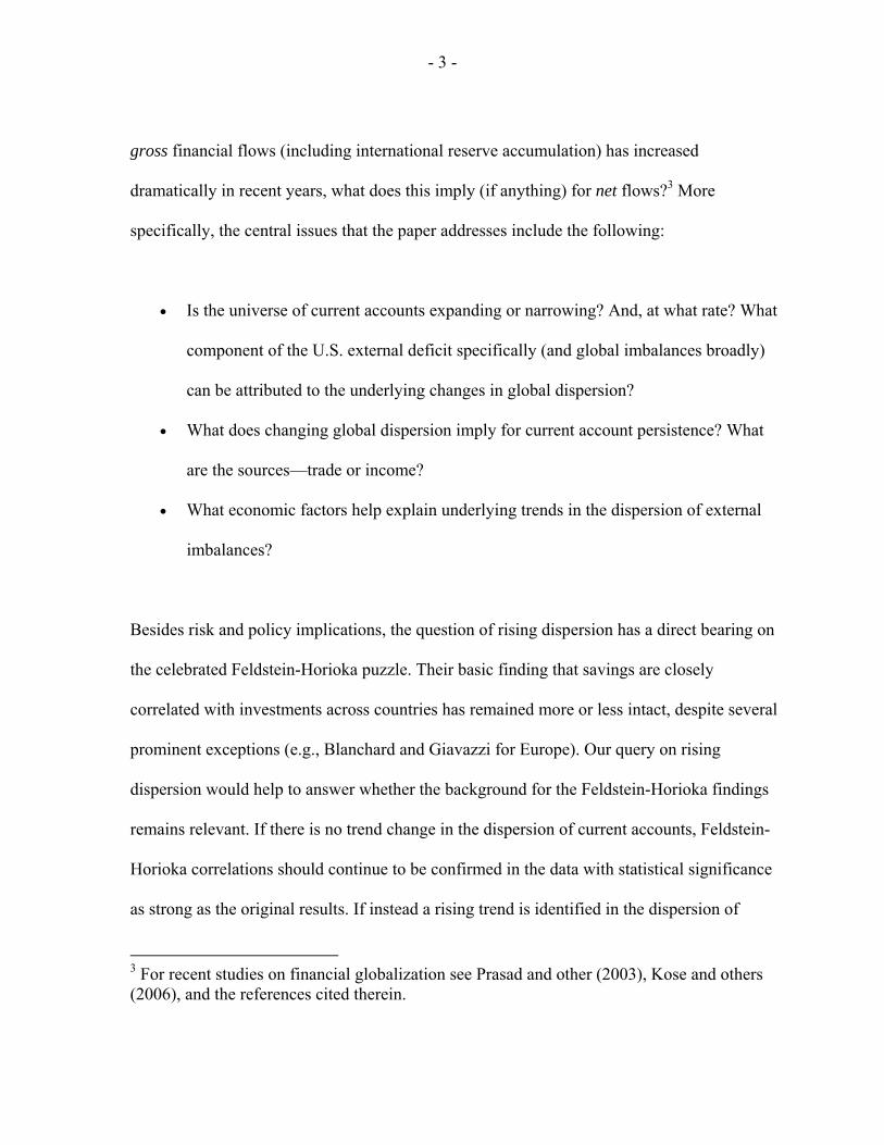
points in time are shown in Figure 1. Kernel density estimates of the cross-sectional

distribution for 101 countries suggest that the universe of current accounts has been generally

expanding. 4 As shown in the figure, the distribution of current accounts shows a steady

increase in dispersion from 1960 to 2004, with the mass of the distribution being less

concentrated in the area around zero and moving further out toward the tails.5 The notable

exception to this progressive pattern of expansion is the year 1980, when presumably the

effects of oil shocks widened the dispersion of current accounts temporarily beyond that seen

in later years. Notice too that the distributions for each year are not exactly centered around

zero (but a small negative value), consistent with the global current account discrepancy.6

4 The kernel estimator for an arbitrary point xi in the distribution is:

∑=

⎥⎦

⎤⎢⎣

⎡ −=

N

j

jii h

XxK

Nhxf

1

1)( ,

where Xj is the jth data observation, N is the number of observations, h is the window size (i.e., the degree of smoothing), and K is the kernel or weighting function. The non-parametric estimates in Figure 1 are based on the Epanechnikov kernel; See Silverman (1986). Results using the less efficient Gaussian kernel (i.e., standard normal) are very similar.

5 Jarque-Bera tests strongly reject normality for each of these years. Skewness in the distribution was found significant for each of these years, except 1960; excess kurtosis (i.e., “fat tails”) was statistically significant throughout.

6 The global current account discrepancy—ususally expressed in dollar terms or in percent of world imports or GDP—has tend to be negative since the early 1970s, reflecting

(continued)

- 6 -

Figure 1. Global Distribution of Current Accounts, 1960-2004

0%

15%

-30 -20 -10 0 10 20 30

Current Accounts(in percent of GDP)

Frequency(in percent)  1960

1970

1990

2004

 1980

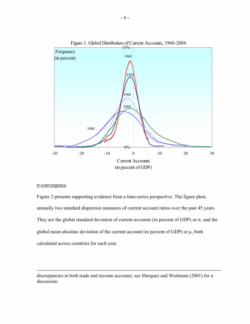
σ-convergence

Figure 2 presents supporting evidence from a time-series perspective. The figure plots

annually two standard dispersion measures of current account ratios over the past 45 years.

They are the global standard deviation of current accounts (in percent of GDP) or σ, and the

global mean absolute deviation of the current account (in percent of GDP) or µ, both

calculated across countries for each year.

discrepancies in both trade and income accounts; see Marquez and Workman (2001) for a discussion.

- 7 -

Two features of the figure are worth noting. First, dispersion shows significant time variation

from year to year. Consistent with the impression from the previous figure, notice the

considerable increase in the global spread around the time of the two major oil shocks in the

mid- and late-1970s. Second, an underlying trend increase in dispersion is apparent,

consistent with the global distributions shown in Figure 1. Specifically, the universe of

current account positions has been expanding on average by almost 2 percent per annum,

measured by its standard deviation.7 This latter finding suggests a lack of so-called “σ-

convergence” in external positions over this time horizon.

Note that both measures are unweighted, treating each country symmetrically. For

comparison, a third measure of dispersion ∑ is shown in the figure by computing the global

sum of current accounts (in absolute value) in percent of world GDP. This is equivalent to a

weighted mean absolute deviation of current accounts (in dollar terms), where country

weights are determined by own GDP (in dollar terms) as a share of world GDP (in dollar

terms). All three measures are highly correlated (with correlation coefficients between (0.60

and 0.95). However, the third measure shows a steeper increase, particularly in recent years,

well ahead of the other (unweighted) measures.8 This corresponds to emergence of “global

7 A regression of the (log) standard deviation on a time trend yields the following results (with corrected standard errors given in parentheses):

33.0;017.04.1)ln( 2/ =++= Rt tGDPCA εσ .

8 Over the sample, the rate of increasing global dispersion is 1½ to 1¾ perent per year on an unweighted basis and 3¼ percent on a weighted basis.

- 8 -

imbalances” where large deficits and surpluses emerged in the largest countries such as the

United States and China.

Figure 2. Global Dispersion of Current Accounts, 1960‐2004(in percent of GDP)

0

5

10

1960 1965 1970 1975 1980 1985 1990 1995 2000 20050

5

10σCA/GDP

Notes: σ denotes global standard deviation of current accounts (in percent of GDP);µ denotes global average of absolute values of current accounts (in percent of GDP);Σ denotes global sum of absolute values of current accounts (in percent of world GDP);

µ|CA/GDP|

Σ|CA|/World GDP

β-convergence

Another convergence perspective—commonly used in the growth literature—is the notion of

“β-convergence.” In the context of current accounts, β-convergence would require that

countries accumulating past imbalances eventually unwind these positions. This would allow

current accounts (and trade balances) globally to converge to more similar values around

- 9 -

zero—i.e., the convergence point.9 For example, countries with a large stock of net external

debt, reflecting flow deficits in the past, would need to run current account surpluses in the

future to pay down the debt or, at least, smaller current account deficits to decrease the share

of debt relative to the overall economy. Comparing the initial net foreign asset ratio to the

average current account ratio in subsequent years, however, provides very little support for

this type of convergence. The cross-country regressions, in fact, show that countries with

larger net indebtedness are more likely to run larger (not smaller) current account deficits in

the years that follow. See figure 3.10 And the results of the cross section regression are:

94;13.0;)05.0(

09.0)36.0(

94.1 20 ==++−= NOBSRvNFACAavg

Moreover, the slope of the line drawn is greater than typical estimates of nominal growth in

GDP, suggesting these subsequent flow imbalances tend to augment the net stock of external

assets or liabilities in relation to the size of the economy. Alternative coefficient estimates

may be more comparable to nominal dollar growth rates. This would imply a reversion to the

9A weaker form of convergence posits that current accounts, but not trade balances nor net foreign asset positions, converge toward balance. This would require that trade (not current account) surpluses be achieved in the years following current account deficits to stabilize the accumulation of net foreign liabilities. Net foreign assets data are based on Lane and Milesi-Ferretti (2001 and 2007).

10 Chinn and Prasad (2002) find a similar effect of net foreign assets on current accounts based on multivariate panel estimation that controls for a wide range of explanatory variables (e.g., demographics, fiscal positions, economic development, etc).

- 10 -

initial ratios of NFA to GDP, but this is still at variance with the notion of a convergence to a

common value (e.g. zero balance). 11

Figure 3. Net Foreign Assets v. Current Accounts(in percent of GDP)

-20

-15

-10

-5

0

5

-100 -50 0 50 100

Initial NFA, 1960 (or earliest available)

Ave

rage

CA

, 196

0-20

03

∪+= 0.53

This result is comparable to the findings of Kraay and Ventura (2000). Using the data from

less than 20 industrial countries, they found that current account imbalances are proportional

to the net external balance sheet positions. In response to an increase in savings, a creditor

country tended to run surplus while a debtor country tended to stay in deficit. They view this

to be the result of a portfolio choice in the presence of a large investment risk. While data

11 Dropping outlier countries with average current account imbalances (net external assets) greater than 10 percent (50 percent) of GDP in absolute terms would slightly lower the coefficient on initial NFA (to 0.06) but raise its significance level (p-value = 3%).

- 11 -

limitation makes it difficult to examine the validity of their prediction for a wider set of

countries, their model is one possible explanation for the result that we find for a very large

set of countries.

To recap, the distributional and convergence properties of current account balances suggest

an expanding universe. The β-convergence results further suggest that countries who have

had current account imbalances historically are the group more likely to run subsequent

current account imbalances (of the same sign) in ensuing periods, leading to further

accumulation of net foreign assets or liabilities.

3. Stationarity & Persistence

We now examine aspects of the time-series properties of current accounts—in particular,

stationarity and persistence. Trehan and Walsh (1991) showed that the stationarity of the

current account is a sufficient condition for the intertemporal budget constraint to hold.12

Stationarity has since been an indirect test of the basic premise of the intertemporal view of

the current account. Thus, this type of behavior would indicate whether the expanding global

dispersion of current accounts has also been compatible with respecting intertemporal budget

constraints.

12 Trehan and Walsh showed that the stationarity of the current account was the necessary and sufficient condition, but the necessity was debated lately by Bohn (2006).

- 12 -

To examine the stationarity and persistence properties of current accounts, a battery of unit

root and stationarity tests were conducted. In particular, the well-known augmented Dickey-

Fuller (ADF) test and non-parametric Phillips-Perron (PP) test for a unit root against a

stationary alternative were applied to the individual country series for the current account

ratio (in percent of GDP). In addition, the Kwiatowski et al (1992) (KPSS) test for

stationarity against a unit root was also used. The corresponding test statistics and

significance levels are shown in the appendix.13

Figure 4 summarizes the rejection and non-rejection rates (in percent) for these unit root

tests. For more straightforward comparisons, the rejection of stationarity under the KPSS test

is reported as a non-rejection of the unit root. Overall, the picture is quite mixed. One test

finds the majority of current accounts to be non-stationary (ADF test), another tests finds the

majority to be stationary (KPSS test), and the third test is split down the middle (PP test).

Individually, for nearly a quarter of the sample (22 of 101), these tests failed to reject both

non-stationarity and stationarity for the same series (see appendix). This finding highlights

two widely-known features of these tests and the time-series data: (1) unit root and

stationarity tests tend to have low power (i.e., fail to reject too often) in finite samples, and

13 In all cases, the model specification includes a constant but no time trend. Including a time trend in the unit root tests marginally increase the number of rejections.

- 13 -

(2) the current account is generally a very persistent series, making it difficult to distinguish

between non-stationary and stationary alternatives over limited time spans.14

Figure 4. Unit Root Test Rejection Rates(Variable = CA/GDP; in percent)

17.8

54.5

75.282.2

45.5

24.8

0

25

50

75

100

ADF PP KPSS

rejectaccept

1/ Variable is CA-to-GDP ratio; for KPSS test, failure to reject stationarity reported as rejection of unit root in the graph. N=101.

1/

For 21 countries—including, notably, the United States and Japan, the tests indicated (at

least, statistically) a non-stationary current account ratio over this time span. That is, the unit

root tests failed to reject non-stationarity and the KPSS test further rejected stationarity. But

for more than half of the sample (55 of 101 countries), at least one of the two unit root tests

reject and the stationarity test accept their respective null hypotheses, suggesting a stationary

series.

14 See Campbell and Perron (1991). A peculiar finding is that for three countries,these low-powered tests rejected both stationarity and non-stationarity for at least one unit root test.

- 14 -

Moreover, on the basis of panel unit root tests (Table 1), non-stationarity is strongly rejected.

The tests were applied to three panels comprising different groups of countries according to

data availability. The first panel comprises data from 1960 to 1998 for 50 countries, the

second panel comprises data from 1971 to 1998 for 82 countries, and the third panel

comprises data from 1980 to 1998 for 94 countries (excluding Kuwait). The null of

nonstationarity is strongly rejected for all possible specifications suggested by Levin and Lin

(1992), Im, Pesaran and Shin (1995), and Breitung (2000); see appendix. Test statistics

reported in the table correspond to specifications without time trend, but a unit root was

rejected for specifications with time trend, too.

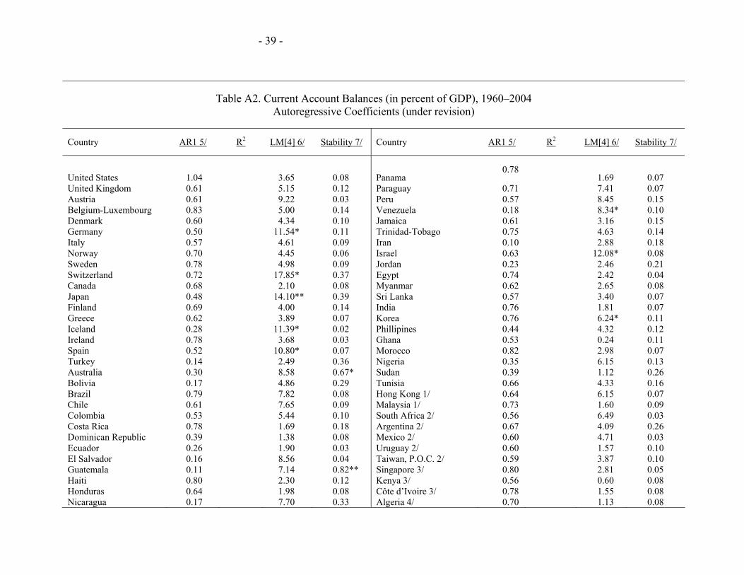
Overall, these various tests suggest that the current account is a stationary but persistent

series. To further highlight this point, simple AR(1) specifications for the current account are

reported in appendix (Table A2). The average autoregressive coefficient across country

estimates is 0.58. From a panel perspective, pooled OLS and fixed effects estimates,

respectively, yield the following equations (with corrected standard errors in parentheses):

59.0;)02.0(

75.0 21 =++= − RCAkCA titit ε (1)

62.0;)01.0(

60.0 21 =++= − RCAkCA titiit ε (2)

Under either specification, there is significant AR(1) coefficient on the lagged current

account, though with panel fixed effects, the degree of inertia is reduced somewhat.

- 15 -

But these specifications are, in a sense, incomplete—failing to recognize a common

component associated with the particular pattern in the movement of global dispersion over

the past several decades. Moreover, the β-convergence results indicate that countries with

non-zero initial NFA positions continue to accumulate assets (liabilities) on a net basis by

running current account surpluses (deficits) in subsequent periods. In other words, countries

tend to run significant imbalances of the same sign (either positive or negative) as in the past.

To introduce this trend feature into the analysis, we include a sign-preserving time trend

(sptrend) constructed as follows:

1( ) *t tsptrend sign CA t−= ; where 111 /)( −−− = ttt CACACAsign . (3)

The time trend specifies increasing surpluses or deficits depending on the sign of the current

account in the previous period. Note too that this sign-preserving trend is also broadly

consistent with preserving current account adding-up, while a simple time trend is not.15

Including this term into the panel fixed effects regression yields:

63.0;)01.0(

59.0)004.0(

01.0 21 =+++= − RCAsptrendkCA tittiit ε (4)

15 Current account adding-up would be more apparent if balances were defined in a common unit, (say) U.S. dollars—but this would raise issues of nominal drift. Using the current account ratio to GDP broadly perserves the level of the current account discrepancy (in percent of GDP) provided that surplus and deficit countries (as respective groups) are of similar economic size.

- 16 -

The trend capturing increasing dispersion is statistically significant (p value = 0.08).16 The fit

of the equation is marginally improved and the persistence parameter (AR1 coefficient) is

smaller, as one would expect.17 In other words, some of the observed persistence in external

balances appears to reflect an underlying trend phenomenon—a slowly increasing global

dispersion. This is perhaps better viewed as an evolving longer-run process occurring over

many decades rather than the inertia in external balances seen from year to year.

Taking an average trend estimate over different specifications, one can examine the extent to

which the recent increase in the U.S. current account deficit is due to this underlying global

trend. Figure 5 shows the observed U.S. current account deficit ratio to GDP (line) and the

long-run contributions (bars) that obtain from equation (4), reflecting the common or global

trend term on average. Accounting for increasing global dispersion goes part way to

explaining the burgeoning U.S. deficit in past years, but clearly the widening imbalance has

gone far beyond these considerations. In level terms, the long-run component (adding the

16 Due to the unbalanced panel, the sign-preserving trend coefficient in (4) is estimated for the vast majority (but not all) countries. Including the full sample (which has countries with only few observations at the end of sample) would reduce the coefficient estimate given the accumulated value of the trend term itself. A “resetting” trend for these countries would raise the point estimate. For further sensitivity analysis, see the following footnote.

17When the sign-preserving trend is constructed using the contemporaneous rather than lagged current account, the trend coefficient is always substantially larger and highly significant; and the AR1 coefficient is also substantially reduced.But this specification is susceptible to simultaneity issues. Across various specifications and samples, the range of trend estimates is roughly between 0.005 to 0.085. As a cross-check, the fitted values and implied rate of increase in global dispersion for a given trend estimate is compared to the rates from the non-parametric estimates disscussed earlier.

- 17 -

trend and either a common or country-specific constant) would narrow but not nearly close

the “gap” with the observed deficit.

Figure 5. U.S. Current Account, 1960-2004(in percent of GDP)

-7

-6

-5

-4

-3

-2

-1

0

1

2

1960 1965 1970 1975 1980 1985 1990 1995 2000-7

-6

-5

-4

-3

-2

-1

0

1

2

U.S. Current Account Balance

Trend Component

4. Dispersion, Persistence, and Openness

We have seen that the cross section dispersion of current accounts has been rising while the

time series of current accounts have remained stationary. In particular, equation (4) based on

sign-preserving trends suggests that the cross-section distribution of long-run average current

accounts (measured by the constant terms in AR(1) regression and the sign-preserving

trends) has been spreading out. What are behind these trends? Are they in fact driven by the

- 18 -

force of globalization, experienced as a rising integration of goods and financial markets

across different countries?

We thus consider two economic variables that are likely to affect the behavior of external

imbalances: openness to trade and financial flows. We measure trade openness by the ratio of

exports and imports to GDP, and financial openness by the Chinn-Ito index, scaled to lie

between 0 and 1 (see the appendix for details). As most economies have been opening up and

increasing external flows in trade and finance, a deterministic time trend will capture a large

part of the common trend toward greater openness. Country-specific measures of openness,

however, will help us to extract more information on the role of openness by exploiting

different speeds toward openness among countries.

Countries with more open trade regimes would find it easier to sell goods produced beyond

the need for domestic consumption and to import goods for which demand exceeds domestic

production. The trade imbalance is the aggregate accumulation of such imbalances over the

whole economy. A country with more open trade regime will thus be more likely to run a

trade imbalance, and also find it easier to finance them given the wider base for international

lending and borrowing.

More directly, countries with more open financial account will find it easier to lend or

borrow to balance its savings capacity and investment need. In addition to enabling countries

to put savings to the most productive use and to finance investment needs in the most

- 19 -

efficient manner, a greater availability of investment and funding opportunities will tend to

stimulate savings and investment, and increase international financial flows further.

To fix ideas on how to incorporate their effects on the dispersion of current accounts, let us

consider the following AR(1) representation of the current account of country i.

1it i it itCA CAµ β ε−= + +

Idiosyncratic shocks itε are uncorrelated across countries and time ( i and t ), and have mean

zero and unit variance ( 2 ( ) 1itσ ε = ), evaluated over i at each point in time. The long-run

average current account, iµ , is allowed to differ across countries. Since the current accounts

have been found to be stationary with its AR(1) coefficients lying between 0 and 1, we

assume that 0 1β< < , and obtain the following MA representation of the current account.

10

lit i it

lCA µ β ε

∞

−=

= + ∑

The global dispersion of current account at time t is

2 2 2 2 2 1 2

0( ) ( ) ( ) (1 ) ( )l

it it l i il

CAσ β σ ε σ µ β σ µ∞

−−

=

= + = − +∑

There are two ways that the global dispersion of current accounts can increase. For one, the

cross-section distribution of the long-run average current account can spread out over time,

thereby increasing the global dispersion of the current account. Alternatively, a rise in the

persistence of current account deviation from its long-run average can increase the observed

- 20 -

global dispersion of current account as the effect of idiosyncratic shocks die out more slowly.

(See Taylor (2001) for suggestive evidence of the latter channel for traditional OECD

countries over a span of 100 years.)

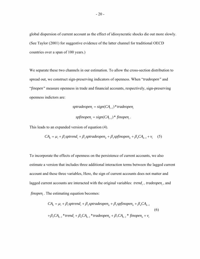
We separate these two channels in our estimation. To allow the cross-section distribution to

spread out, we construct sign-preserving indicators of openness. When “tradeopen” and

“finopen” measure openness in trade and financial accounts, respectively, sign-preserving

openness indictors are:

1( )*t t tsptradeopen sign CA tradeopen−=

1( )*t t tspfinopen sign CA finopen−= .

This leads to an expanded version of equation (4).

1 2 3 4 1it i t it it it tCA sptrend sptradeopen spfinopen CA vµ β β β β −= + + + + + (5)

To incorporate the effects of openness on the persistence of current accounts, we also

estimate a version that includes three additional interaction terms between the lagged current

account and these three variables, Here, the sign of current accounts does not matter and

lagged current accounts are interacted with the original variables: ttrend , ttradeopen , and

tfinopen . The estimating equation becomes:

1 2 3 4 1

5 1 6 1 7 1* * *

it i t it it it

it t it it it it t

CA sptrend sptradeopen spfinopen CA

CA trend CA tradeopen CA finopen v

µ β β β β

β β β

−

− − −

= + + + +

+ + + + (6)

- 21 -

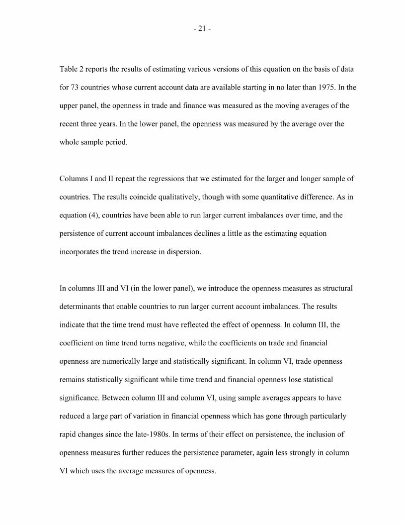
Table 2 reports the results of estimating various versions of this equation on the basis of data

for 73 countries whose current account data are available starting in no later than 1975. In the

upper panel, the openness in trade and finance was measured as the moving averages of the

recent three years. In the lower panel, the openness was measured by the average over the

whole sample period.

Columns I and II repeat the regressions that we estimated for the larger and longer sample of

countries. The results coincide qualitatively, though with some quantitative difference. As in

equation (4), countries have been able to run larger current imbalances over time, and the

persistence of current account imbalances declines a little as the estimating equation

incorporates the trend increase in dispersion.

In columns III and VI (in the lower panel), we introduce the openness measures as structural

determinants that enable countries to run larger current account imbalances. The results

indicate that the time trend must have reflected the effect of openness. In column III, the

coefficient on time trend turns negative, while the coefficients on trade and financial

openness are numerically large and statistically significant. In column VI, trade openness

remains statistically significant while time trend and financial openness lose statistical

significance. Between column III and column VI, using sample averages appears to have

reduced a large part of variation in financial openness which has gone through particularly

rapid changes since the late-1980s. In terms of their effect on persistence, the inclusion of

openness measures further reduces the persistence parameter, again less strongly in column

VI which uses the average measures of openness.

- 22 -

We examine the effects of these variables on the persistence parameter (AR1 coefficient). No

strong prior applies to the direction of their effects. It is tempting to presume that a greater

availability of financing will lead to a higher persistence of the shocks to current account, for

countries will be able to finance their current account deficits more easily. However, the

relaxation of financial constraints can also lead countries to fund their needs more quickly

but at a larger scale. For example, a Solovian developing country that needs a large

development financing will borrow a large amount in the beginning, if she can. Such

response will imply a lower persistence of current account shocks and a larger dispersion of

current account imbalances across countries. To summarize, a larger value of the persistence

parameter is consistent with a more gradual financing, while a smaller value is consistent

with a more rapid financing.

Starting with a regression that only uses time trend (column IV), the persistence parameter is

found to have been declining over time. Countries are also found to have been able to run

larger current account imbalances—deficit or surplus—over time. When we allow openness

measures to affect persistence (columns V and VII), we uncover an interesting contrast in the

effects of trade and financial openness. Trade openness, if any, increases the persistence of

current account imbalance while financial openness reduces the persistence. And the effect of

financial openness remains statistically significant even when the openness is measured by

the average over the whole sample period. Most interesting is the joint effect of financial

openness on persistence and the dispersion of long-run average current accounts. A

financially more open—better integrated—country appears to be able to run a larger

- 23 -

imbalance, but over a shorter duration. This is consistent with the possibility that financially

better integrated countries can meet its international financing or investment need more

quickly.

These findings are confirmed in Table 3, where the same relationships as in Table 2 were

estimated by popular GMM estimates, considering the presence of lagged dependent

variables on the right hand side. Trade openness is found to increase the persistence of

current account imbalances, whereas financial openness is found to clearly decrease the

persistence of current account imbalances.

5. Concluding Remarks

Examining current accounts for a wide spectrum of countries over the past four and a half

decades, we can summarize our key findings or “stylized facts” as follows:

• The universe of current accounts has been expanding over the past half century.

Based on a variety of measures and methodologies, the global constellation of

external current account positions has markedly widened over time. While dispersion

can vary significantly from year to year—ostensibly in response to large international

shocks, there is a steady, underlying rate of expansion of around 2 to 3 percent per

year.

• In other words, in a context where global gross financial flows have grown rapidly,

net flows have also increased (on a sustained basis) to individual countries. And sign

reversals in the current account are occasional, but not frequent. Reflecting this

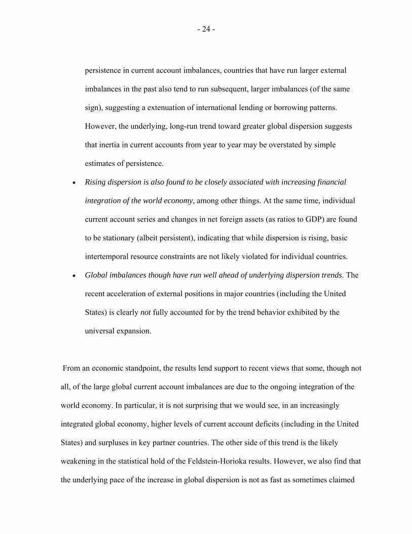
- 24 -

persistence in current account imbalances, countries that have run larger external

imbalances in the past also tend to run subsequent, larger imbalances (of the same

sign), suggesting a extenuation of international lending or borrowing patterns.

However, the underlying, long-run trend toward greater global dispersion suggests

that inertia in current accounts from year to year may be overstated by simple

estimates of persistence.

• Rising dispersion is also found to be closely associated with increasing financial

integration of the world economy, among other things. At the same time, individual

current account series and changes in net foreign assets (as ratios to GDP) are found

to be stationary (albeit persistent), indicating that while dispersion is rising, basic

intertemporal resource constraints are not likely violated for individual countries.

• Global imbalances though have run well ahead of underlying dispersion trends. The

recent acceleration of external positions in major countries (including the United

States) is clearly not fully accounted for by the trend behavior exhibited by the

universal expansion.

From an economic standpoint, the results lend support to recent views that some, though not

all, of the large global current account imbalances are due to the ongoing integration of the

world economy. In particular, it is not surprising that we would see, in an increasingly

integrated global economy, higher levels of current account deficits (including in the United

States) and surpluses in key partner countries. The other side of this trend is the likely

weakening in the statistical hold of the Feldstein-Horioka results. However, we also find that

the underlying pace of the increase in global dispersion is not as fast as sometimes claimed

- 25 -

and has bounds, indicating that a sizable part of today’s global imbalances is likely in excess

(relative to the underlying trend) and would probably be unwound to a significant degree.

Some movements in that direction appear to have finally started in the United States, while

the counterpart movements are less evenly distributed.

- 26 -

REFERENCES Bernanke, Ben, 2005, “Remarks at the Homer Jones Lecture.” St. Louis, MO, April 14, 2005. Blanchard, Olivier J. and Giavazzi, Francesco, "Current Account Deficits in the Euro Area. The End of the Feldstein Horioka Puzzle?" (2002) Blanchard, Olivier, Francesco Giavazzi, and Filipa Sa, The U.S. Current Account and the Dollar, NBER Working Paper No 11137, 2005/ BPEA 2006. Bohn, Henning, 2005, “Are Stationarity and Cointegration Restrictions Necessary for the Intertemporal Budget Constraint?” mimeo, Univeristy of California at Santa Barbara. Campbell, John Y. and Pierre Perron, “Pitfalls and Opportunities: What Macroeconomists Should Know about Unit Roots,” NBER Working Paper T0100 (April). Chinn, Menzie D. and Hiro Ito, 2005, “What Matters for Financial Development? Capital Controls, Institutions, and Interactions,” Journal of Development Economics (forthcoming). Chinn, Menzie D. and Jaewoo Lee, 2005, “Three Current Account Balances: A Semi-Structuralist Interpretation,” NBER Working Paper . Faruqee, H., D. Laxton, D. Muir and P. Pesenti, 2006a, “Smooth Landing or Crash? Model-based Scenarios of Global Current Account Rebalancing” =in R. Clarida (ed.), G7 Current Account Imbalances: Sustainability and Adjustment, NBER conference volume: University of Chicago Press. Faruqee, H., D. Laxton, D. Muir and P. Pesenti, 2006b, “Would Protectionism Defuse Global Imbalances and Spur Economic Activity? A Scenario Analysis,” NBER Working Paper 12704 (November). Feldstein, Martin and Charles Horioka, 1980, "Domestic Saving and International Capital Flows", Economic Journal 90: 314-329 Ghironi, Fabio, Jaewoo Lee and Alessandro Rebucci, 2007 “The Valuation Channel of External Adjustment,” NBER WP 12937. Gourinchas, Pierre-Olivier and Helene Rey, 2005, “From World Banker to World Venture Capitalist: The U.S. External Adjustment and the Exorbitant Privilege.” Paper presented at the NBER conference, “G-7 Current Account Imbalances: Sustainability and Adjustment,” Newport, June 1–2. Greenspan, Alan, 2005, “Current Account.” Presentation at Advancing Enterprise 2005 Conference, London, February 4, 2005.

- 27 -

IMF, 2005, World Economic Outlook (Washington, D.C., September). Kose, M. Ayhan, Eswar S. Prasad, Kenneth Rogoff and Shang-Jin Wei, 2006, “Financial Globalization: A Reappraisal,” IMF Working Paper 06/189. Kraay, Art and Jaume Ventura, 2000, “Current Accounts in Debtor and Creditor Countries,” Quarterly Journal of Economics. Krugman, Paul, 1991. “Introduction,” in: Bergsten, C. F. (Eds.), International Adjustment and Financing: The Lessons of 1985–1991, Institute for International Economics, Washington, D.C., pp. 3-12. Lane, Philip and Gian Maria Milesi-Ferretti, 2001, “The External Wealth of Nations: Measures of Foreign Assets and Liabilities in Industrial and Developing Countries” Journal of International Economics 55 no. 2, December 2001, 263-94. Lane, Philip and Gian Maria Milesi-Ferretti, 2007, “The External Wealth of Nations Mark II: Revised and Extended Estimates of Foreign Assets and Liabilities,” (joint with Philip Lane), Journal of International Economics 73 (November 2007), 223-250. Marquez, Jaime and Workman, Lisa, 2001, "Modeling the IMF's Statistical Discrepancy in the Global Current Account", IMF Staff Papers, 2001, vol. 48, issue 3 (September). Obstfeld, Maurice, and Kenneth Rogoff, 2004, “The Unsustainable US Current Account Position Revisited,” NBER Working Paper No. 10869. Prasad, Eswar S., Kenneth Rogoff, Shang-Jin Wei, and M. Ayhan Kose, 2003, Effects of Financial Globalization on Developing Countries: Some Empirical Evidence, IMF Occasional Paper No. 220 (Washington: International Monetary Fund). Taylor, Alan, 2001, “A Century of Current Account Dynamics,” Journal of International Money and Finance. Trehan, Bharat and Carl E. Walsh, 1991, “Testing Intertemporal Budget Constraints: Theory and Application to U.S. Federal Budget and Current Account Deficits,” Journal of Money, Credit, and Banking, 23 (2), pp. 206-23.

- 28 -

Appendix I. Data Description

The main variable is the ratio of the current account to the GDP, both of which were obtained

from various issues of International Financial Statistics (IMF) and World Development

Indicator (World Bank). The capital account liberalization index was developed by Chinn

and Ito (2005), and is the first principal component of several variables that reflect the ease

of cross-border financial transactions. In our estimation, the index was normalized to take a

value between 0 and 1, increasing with the liberalization of capital account regime. For each

value of Chinn-Ito index itCI , our indicator is defined as follows.

{ }{ } { }

it itit

it it

CI Min CIfinopen

Max CI Min CI−

=−

Descriptive statistics for the ratio of the current account to GDP show:

• Unconditional means in more than three-quarters (74 out of 94) of the countries statistically different from zero (p=0.05 or higher); see Table A0.

• Conditional means in more than half of the countries (64 out of 94), based country constants (i.e., fixed effects), are significantly different from 0 (p= 0.10 or higher).

• For higher moments, evidence of skewness or excess kurtosis (“fat tails”) was found in 28 out of 94 countries (i.e., 30 percent of sample).

- 29 -

Appendix II. Alternative Measures of External Positions and Their Behavior

A related but distinct measure is the change in net foreign assets (NFA). It essentially differs

from the current account by the amount of capital gains (valuation change), which is driven

by asset price fluctuations, including exchange rate variations. Since these asset price

movements are broadly described as a random walk, the change in NFA will contain a much

larger white-noise component and exhibit smaller persistence than the current account. This

is indeed confirmed by the data, as summarized in the following two charts. Note that due to

data limitations regarding NFA, the sample size is smaller.

First, the change in NFA (in percent of GDP) is subjected to the same battery of stationarity

and unit root tests as for the current account, summarized in Figure 4. The test results

uniformly show a higher rejection rate of non-stationarity. See Figure A1. Second, for the

change in the ratio of NFA to GDP—i.e., ∆(NFA/y)— the indications toward stationarity are

even stronger; see Figure A2. Changes in the ratio also include a growth term (related to the

change in the scaling variable GDP). This helps toward finding stationarity in the ratio given

that GDP (i.e., the denominator) is growing over time. Excluding the growth factor term (by

considering ∆NFA/y) weakens the stationarity finding, but does not overturn it. That is, the

∆NFA concept appears to be much more stationary (less persistent) series than CA.

- 30 -

Figure A1. Unit Root Tests Rejection Rates(variable = ∆NFA/GDP; in percent)

49.4

77.8

87.8

50.6

22.2

12.2

0

25

50

75

100

ADF PP KPSS

rejectaccept

1/ Variable is change in NFA as a ratio to GDP; for KPSS test, failure to reject stationarity reported as rejection of unit root in the graph. N=81.

1/

Appendix III. Expanding Dispersion and Financial Market Integration

Considering the pivotal role of the financial openness in expanding the global dispersion of

current accounts, we present an illustrative (steady-sate) model where the ongoing integration

in international financial markets increases the global dispersion of current accounts. Some

form of heterogeneity is the necessary condition for global dispersion, and we introduce the

heterogeneity in the discount rate. Combined with a small cost of financial intermediation,

which represents financial market friction, we generate a non-degenerate steady-state

distribution of net foreign assets. Further introducing growth in aggregate output, we show

Figure A2. Unit Root Test Rejection Rates(variable = ∆(NFA/GDP); in percent)

69.1

88.994.5

30.9

11.15.5

0

25

50

75

100

ADF PP KPSS

rejectaccept

1/ Variable is change in NFA-to-GDP ratio; for KPSS test, failure to rejectstationarity reported as rejection of unit root in the graph. N=81.

1/

- 31 -

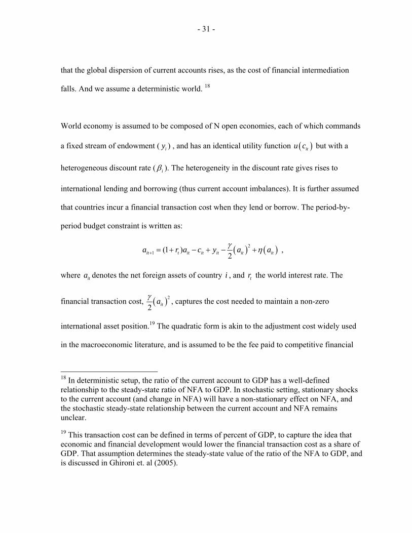
that the global dispersion of current accounts rises, as the cost of financial intermediation

falls. And we assume a deterministic world. 18

World economy is assumed to be composed of N open economies, each of which commands

a fixed stream of endowment ( iy ) , and has an identical utility function ( )itu c but with a

heterogeneous discount rate ( iβ ). The heterogeneity in the discount rate gives rises to

international lending and borrowing (thus current account imbalances). It is further assumed

that countries incur a financial transaction cost when they lend or borrow. The period-by-

period budget constraint is written as:

( ) ( )21 (1 )

2it t it it it it ita r a c y a aγ η+ = + − + − + ,

where ita denotes the net foreign assets of country i , and tr the world interest rate. The

financial transaction cost, ( )2

2 itaγ , captures the cost needed to maintain a non-zero

international asset position.19 The quadratic form is akin to the adjustment cost widely used

in the macroeconomic literature, and is assumed to be the fee paid to competitive financial

18 In deterministic setup, the ratio of the current account to GDP has a well-defined relationship to the steady-state ratio of NFA to GDP. In stochastic setting, stationary shocks to the current account (and change in NFA) will have a non-stationary effect on NFA, and the stochastic steady-state relationship between the current account and NFA remains unclear.

19 This transaction cost can be defined in terms of percent of GDP, to capture the idea that economic and financial development would lower the financial transaction cost as a share of GDP. That assumption determines the steady-state value of the ratio of the NFA to GDP, and is discussed in Ghironi et. al (2005).

- 32 -

intermediaries when international financial position is adjusted away from the zero balance.

The fees paid to competitive intermediaries are distributed back to each country

( ( ) ( )2

2it ita aγη = ) ex post, and thus financial frictions affect the ex-ante decision making of

each country without draining global resources.

The first condition for each country’s consumption-saving choice is:

( ) ( ) ( ) ( )( )11 1t t

i it i it t itu c u c r aβ β γ++′ ′= + − (7)

In the steady state, 1it it ic c c+ = = , and equation (7) simplifies to 1i ir aβ γ= + − and the net

foreign asset position is determined by the difference between the world interest rate and the

subjective discount rate:

1 11ii

a rγ β

⎛ ⎞= + −⎜ ⎟

⎝ ⎠

The world interest rate is determined at a level that equates the global demand and supply of

assets: 1

0N

ii

a=

=∑ :

1

11N

i i

rβ=

+ = ∑

In a no-growth economy just described, the steady-state current account remains in zero

balance and there is no dispersion in current accounts. Introducing economic growth leads to

a steady-state dispersion in current accounts. Now assume that each country’s population

grows at the same rate g . The aggregate output of a country at time t becomes:

- 33 -

(1 )tit iY g y= + , normalizing the time-0 population at unity. Denoting the aggregate net

foreign assets by a capitalized letter, itA , the change in the ratio of net foreign assets to GDP

can be rewritten in terms of the current account as follows.

( )1 1 1 1

1 1 1

1 1it it it it it it it

it it it it it it

A A A A A A CAg gY Y Y Y Y Y

+ + + +

+ + +

−− = − + + = − +⎡ ⎤⎣ ⎦

In the steady state with the constant ratio of the aggregate net foreign assets to GDP,

1

1 1Ni i

iii i i i

CA A gg gaY Y γ β β=

⎡ ⎤⎛ ⎞ ⎛ ⎞ ⎛ ⎞= = = −⎢ ⎥⎜ ⎟ ⎜ ⎟ ⎜ ⎟

⎝ ⎠ ⎝ ⎠ ⎝ ⎠⎣ ⎦∑

A tighter integration of international financial markets is represented as a decline in γ , which

lowers the cost of international financial transactions. This will increase the dispersion in the

ratio of current account to GDP.

- 34 -

Table 1. Stationarity of Current Accounts (current accounts in percent of GDP)

[To be updated]

Panel Unit Root Test

Country Group LL1/ IPS2/ Breitung3/

Small Group 4/ -19.37** -17.66** -11.21** -13.81** Medium Group 5/ -20.10** -16.85** -10.33** -14.28** Large Group 6/ -17.64** -13.55** -8.87** -8.32**

1/ Levin and Liu (1992). For each group, tests with time and individual fixed effects were reported. 2/ Inn, Pesaran, and Shin (1997). 3/ Breitung (2000) 4/ 50 countries, 1960–1998 5/ 82 countries, 1971-1998 6/ 94 countries, 1980–1998 An asterisk * (**) denotes statistical significance at 5(1) percent.

- 35 -

I II III IV V

CA(-1) 0.443 ** 0.403 ** 0.279 ** 0.749 ** 0.861 **(0.017) (0.019) (0.023) (0.054) (0.101)

CA(-1)*TimeTrend -0.012 ** -0.014 **(0.002) (0.003)

CA(-1)*TrOpen 0.177 *(0.090)

CA(-1)*FinOpen -0.433 **(0.065)

SPTrend 0.032 ** -0.028 * 0.043 ** 0.001(0.006) (0.015) (0.006) (0.019)

SPTrOpen 2.183 ** -0.276(0.521) (0.664)

SPFinOpen 1.055 * 2.474 **(0.607) (0.682)

VI VII

CA(-1) 0.359 ** 0.918 **(0.020) (0.087)

CA(-1)*TimeTrend -0.009 **(0.002)

CA(-1)*TrOpenAvg 0.120(0.084)

CA(-1)*FinOpenAvg -0.602 **(0.057)

SPTrend 0.006 0.020(0.010) (0.012)

SPTrOpenAvg 1.296 ** -1.020 *(0.396) (0.501)

SPFinOpenAvg -0.018 1.787 **(0.517) (0.575)

Statistically significant at 5 percent (**) and 10 percent (*).All regressions included country fixed effects. Based on the sample of 73 countries whose current account data were available starting before 1975.

Table 2. Evolution of Current Account Dynamics(1971-2004)

- 36 -

I II III IV V

CA(-1) 0.341 ** 0.290 ** 0.188 ** 1.038 ** 1.340 **(0.001) (0.055) (0.002) (0.010) (0.016)

CA(-1)*TimeTrend -0.027 ** -0.023 **(0.002) (0.001)

CA(-1)*TrOpen 0.020(0.035)

CA(-1)*FinOpen -0.544 **(0.018)

SPTrend 0.055 ** -0.094 ** 0.081 ** -0.011 **(0.001) (0.005) (0.002) (0.005)

SPTrOpen 4.791 ** -0.217(0.181) (0.273)

SPFinOpen 3.454 ** 3.960 **(0.033) (0.215)

VI VII

CA(-1) 0.180 ** 0.912 **(0.002) (0.014)

CA(-1)*TimeTrend -0.021 **(0.001)

CA(-1)*TrOpenAvg 0.423 **(0.010)

CA(-1)*FinOpenAvg -0.591 **(0.010)

SPTrend -0.110 ** 0.041 **(0.002) (0.009)

SPTrOpenAvg 4.963 ** -1.973 **(0.148) (0.221)

SPFinOpenAvg 3.667 ** 4.294 **(0.070) (0.120)

Statistically significant at 5 percent (**) and 10 percent (*).All regressions included country fixed effects. Based on the sample of 73 countries whose current account data were available starting before 1975.

Table 3. Evolution of Current Account Dynamics -- GMM Estimates(1971-2004)

Version: 4/23/2008

Table A1. Current Account Balances (in percent of GDP), 1960–2004 Stationarity Tests (under revision)

Country ADF 1/ PP 2/ KPSS 3/ Country ADF 1/ PP 2/ KPSS 3/

United States 0.21 -0.15 1.16* Argentina -2.24 -3.45* 0.13 United Kingdom -3.11* -2.59 0.45 Taiwan -1.70 -2.60 0.400 Austria -3.03* -3.04* 0.12 Côte d’Ivoire -1.47 -2.39 0.32 Denmark -2.18 -1.97 0.85* Kenya -2.40 -3.95* 0.30 Germany -2.15 -2.42 0.08 Uruguay -2.38 -3.24* 0.16 Italy -2.90 -3.05* 0.21 Algeria -0.75 -2.64 0.62* Norway -1.76 -1.46 0.97* Mauritius -2.52 -3.47* 0.15 Sweden -0.07 -0.24 0.56* Benin -2.47 -4.84* 0.10 Switzerland -0.36 -1.09 1.40* Togo -2.29 -4.05* 0.43 Canada -1.06 -1.81 0.49* Indonesia -1.67 -2.47 0.52* Japan -1.90 -2.74 0.98* Thailand -2.05 -2.14 0.43 Finland -1.39 -1.58 0.66* Uganda -1.49 -4.11* 0.94* Greece -2.69 -3.21* 0.22 France -2.31 -2.77 0.53* Iceland -3.23* -4.72* 0.10 Netherlands -2.75 -3.07* 0.25 Ireland -1.64 -2.08 0.58* New Zealand -3.05* -3.41* 0.11 Spain -3.92* -3.25* 0.25 Saudi Arabia -1.25 -2.14 0.40 Turkey -2.32 -4.75* 0.13 Pakistan -0.87 -2.68 0.55* Australia -1.60 -2.80 0.87* Gabon -1.81 -3.37* 0.19 South Africa -3.57* -3.48* 0.17 Niger -2.83 -2.56 0.47* Bolivia -1.85 -4.43* 0.24 Senegal -2.24 -2.76 0.32 Brazil -2.05 -2.20 0.13 Gambia -2.64 -2.88 0.20 Chile -1.41 -3.08* 0.21 Madagascar -2.67 -5.10* 0.11 Costa Rica -2.19 -3.04* 0.46 Hungary -1.53 -3.18* 0.33 Dominican Republic -2.44 -4.73* 0.31 Congo -0.91 -3.16* 0.33 El Salvador -3.42* -5.51* 0.07 Romania -1.18 -2.35 0.39 Guatemala -2.13 -4.15* 1.09* Portugal -1.31 -2.90 0.18 Haiti -1.84 -2.31* 0.17 Papa New Guinea -1.02 -2.24 0.42

Table A1 (continued). Current Account Balances (in percent of GDP), 1960–2004 Stationarity Tests (under revision)

Country ADF 1/ PP 2/ KPSS 3/ Country ADF 1/ PP 2/ KPSS 3/

- 38 -

Honduras -2.87 -3.57* 0.28 Bangladesh -1.48 -2.62 0.85* Mexico -3.28* -3.49* 0.06 Mauritania -1.44 -2.48 0.41 Panama -2.22 -2.99* 0.26 Oman -1.56 -3.81* 0.24 Paraguay -2.75 -2.98* 0.20 Burkina Faso -0.45 -2.11 0.56* Peru -4.29* -3.80* 0.26 Bahrain -3.35* -2.79 0.18 Venezuela -0.07 -4.27* 0.20 Kuwait -2.55 -4.69* 0.23 Jamaica -2.28 -3.32* 0.10 Bostwana -1.91 -2.57 0.61* Trinidad y Tobago -3.06* -3.02* 0.36 Lesotho -1.53 -2.53 0.40 Israel -2.08 -3.19* 0.39 Ecuador -2.45 -4.08* 0.41 Jordan -3.40* -4.55* 0.11 Nepal -0.67 -1.64 0.28 Egypt -1.73 -2.26 0.68* Poland -1.80 -2.71 0.32 Myanmar -2.63 -3.04* 0.42 Cameroon -2.00 -4.67* 0.41 Sri Lanka -3.04* -3.73* 0.22 C. African Rep. -2.82 -5.64* 0.14 India -2.11 -2.32 0.18 Zimbabwe -2.65 -3.41* 0.08 Korea -1.28 -2.81 0.68* Cambodia -3.47* -3.83* 0.09 Philippines -1.70 -2.43 0.26 Lao P.D. Rep. -3.40* -2.86 0.13 Ghana -2.25 -4.26* 0.15 Namibia -3.12* -4.39* 0.41 Morocco -1.46 -2.35 0.34 Albania -1.88 -4.05* 0.49* Nigeria -2.44 -4.86* 0.20 Bulgaria -1.44 -3.09* 0.43 Sudan -1.81 -3.43* 0.41 China P.R.: Mainland -1.81 -2.74 0.41 Tunisia -3.12* -3.14* 0.27 Mongolia -1.47 -1.27 0.61* Colombia -3.64* -3.44* 0.05 Moldova -1.78 -3.08* 0.13 Hong Kong -2.48 -3.19* 0.29 Russia -1.01 -1.72 0.40 Malaysia -2.24 -2.46 0.28

1/ Augmented Dickey-Fuller t-test statistic for unit root against level stationary alternative; lag length chosen based on Schwarz BIC. 2/ Phillips-Perron Zt test statistic for unit root against level stationary alternative. 3/ Kwiatowski, Phillips, Schmidt & Shin (1992) η(µ) test statistic for level stationarity against non-stationary alternative. An asterisk * denotes statistical significance at the 5 percent level.

- 39 -

Table A2. Current Account Balances (in percent of GDP), 1960–2004 Autoregressive Coefficients (under revision)

Country AR1 5/ R2 LM[4] 6/ Stability 7/ Country AR1 5/ R2 LM[4] 6/ Stability 7/

United States 1.04 3.65 0.08 Panama 0.78

1.69 0.07 United Kingdom 0.61 5.15 0.12 Paraguay 0.71 7.41 0.07 Austria 0.61 9.22 0.03 Peru 0.57 8.45 0.15 Belgium-Luxembourg 0.83 5.00 0.14 Venezuela 0.18 8.34* 0.10 Denmark 0.60 4.34 0.10 Jamaica 0.61 3.16 0.15 Germany 0.50 11.54* 0.11 Trinidad-Tobago 0.75 4.63 0.14 Italy 0.57 4.61 0.09 Iran 0.10 2.88 0.18 Norway 0.70 4.45 0.06 Israel 0.63 12.08* 0.08 Sweden 0.78 4.98 0.09 Jordan 0.23 2.46 0.21 Switzerland 0.72 17.85* 0.37 Egypt 0.74 2.42 0.04 Canada 0.68 2.10 0.08 Myanmar 0.62 2.65 0.08 Japan 0.48 14.10** 0.39 Sri Lanka 0.57 3.40 0.07 Finland 0.69 4.00 0.14 India 0.76 1.81 0.07 Greece 0.62 3.89 0.07 Korea 0.76 6.24* 0.11 Iceland 0.28 11.39* 0.02 Phillipines 0.44 4.32 0.12 Ireland 0.78 3.68 0.03 Ghana 0.53 0.24 0.11 Spain 0.52 10.80* 0.07 Morocco 0.82 2.98 0.07 Turkey 0.14 2.49 0.36 Nigeria 0.35 6.15 0.13 Australia 0.30 8.58 0.67* Sudan 0.39 1.12 0.26 Bolivia 0.17 4.86 0.29 Tunisia 0.66 4.33 0.16 Brazil 0.79 7.82 0.08 Hong Kong 1/ 0.64 6.15 0.07 Chile 0.61 7.65 0.09 Malaysia 1/ 0.73 1.60 0.09 Colombia 0.53 5.44 0.10 South Africa 2/ 0.56 6.49 0.03 Costa Rica 0.78 1.69 0.18 Argentina 2/ 0.67 4.09 0.26 Dominican Republic 0.39 1.38 0.08 Mexico 2/ 0.60 4.71 0.03 Ecuador 0.26 1.90 0.03 Uruguay 2/ 0.60 1.57 0.10 El Salvador 0.16 8.56 0.04 Taiwan, P.O.C. 2/ 0.59 3.87 0.10 Guatemala 0.11 7.14 0.82** Singapore 3/ 0.80 2.81 0.05 Haiti 0.80 2.30 0.12 Kenya 3/ 0.56 0.60 0.08 Honduras 0.64 1.98 0.08 Côte d’Ivoire 3/ 0.78 1.55 0.08 Nicaragua 0.17 7.70 0.33 Algeria 4/ 0.70 1.13 0.08

- 40 -

Table A2 (continued). Current Account Balances (in percent of GDP), 1960–2004 Autoregressive Coefficients (under revision)

Country AR1 5/ R2 LM[4] 6/ Stability 7/ Country AR1 5/ R2 LM[4] 6/ Stability 7/

Mauritius 4/ 0.65 2.35 0.20 Bangladesh 12/ 0.69 5.85 0.26 Benin 5/ 0.27 1.46 0.08 Mauritania 12/ 0.64 2.32 0.07 Togo 5/ 0.27 2.35 0.11 Bahrain 13/ 0.89 6.20 0.23 Indonesia 6/ 0.49 0.95 0.09 Kuwait 13/ 0.22 0.23 0.61 Thailand 6/ 0.89 4.39 0.09 Oman 13/ 0.04 0.19 0.13 Uganda 6/ 0.04 7.66 0.94** Botswana 13/ 0.28 6.37 0.10 France 7/ 0.65 2.26 0.88** Lesotho 13/ 0.70 4.17 0.23 Netherlands 7/ 0.62 4.31 0.48* Nepal 14/ 0.81 0.89 0.89 New Zealand 7/ 0.52 2.54 0.18 Poland 14/ 0.63 1.66 0.34 Saudi Arabia 7/ 0.72 1.62 0.03 Albania 15/ 0.16 6.76 0.08 Pakistan 7/ 0.65 0.60 0.10 Bulgaria 15/ -0.06 5.82 0.03 Syrian Arab Rep. 8/ 0.13 9.73* 0.20 Gabon 8/ 0.43 0.88 0.18 Niger 8/ 0.68 3.98 0.07 Average 0.35 …. …. Senegal 8/ 0.66 4.50 0.09 Pooled OLS 0.47 …. …. Gambia 9/ 0.52 8.39 0.03 Panel Fixed Effects 0.50 …. …. Madagascar 9/ 0.17 7.32 0.08 Hungary 9/ 0.55 2.85 0.09 Congo, Republic of 10/ 0.05 2.82 0.11 Romania 10/ 0.20 1.91 0.06 Portugal 11/ 0.62 3.60 0.05 Papua New Guinea 11/ 0.75 2.70 0.18 1/ Estimation period 1965-2004. 2/ Estimation period 1970-2004. 3/ Estimation period 1975-2004. 4/ Estimation period 1980-2004. 5/ Coefficient on first-order autoregressive term. 6/ Test statistic from Lagrange Multiplier test against 4th-order serial correlation in the residuals. 7/ Denotes Hansen test for stability of the AR1 coefficient An asterisk * (**) denotes statistical significance at the 5 (1) percent level.