global banking glut and loan risk premium - imf · global banking glut and loan risk premium∗...
TRANSCRIPT
Global Banking Glut and Loan Risk Premium
Hyun Song Shin
Princeton University
Paper presented at the 12th Jacques Polak Annual Research Conference
Hosted by the International Monetary Fund
Washington, DC─November 10–11, 2011
The views expressed in this paper are those of the author(s) only, and the presence
of them, or of links to them, on the IMF website does not imply that the IMF, its
Executive Board, or its management endorses or shares the views expressed in the
paper.
1122TTHH JJAACCQQUUEESS PPOOLLAAKK AANNNNUUAALL RREESSEEAARRCCHH CCOONNFFEERREENNCCEE NNOOVVEEMMBBEERR 1100––1111,, 22001111
Global Banking Glut
and Loan Risk Premium∗
Hyun Song Shin
Princeton University
November 6, 2011
2011 Mundell-Fleming LectureConference Draft
Abstract
European global banks intermediating US dollar funds are important in influencing
credit conditions in the United States. US dollar-denominated assets of banks outside the
US are comparable in size to the total assets of the US commercial bank sector, but the
large gross cross-border positions are masked by the netting out of the gross assets and
liabilities. As a consequence, current account imbalances do not reflect the influence of
gross capital flows on US financial conditions. This paper pieces together evidence from
a global flow of funds analysis, and develops a theoretical model linking global banks and
US loan risk premiums. The culprit for the easy credit conditions in the United States up
to 2007 may have been the “Global Banking Glut” rather than the “Global Savings Glut”.
∗Draft of the Mundell-Fleming Lecture, prepared for the 2011 IMF Annual Research Conference, November10-11, 2011. I thank Viral Acharya, James Aitken, Carol Bertaut, Claudio Borio, Michael Chui, Stijn Claessens,
Pierre-Olivier Gourinchas, Dong He, Haizhou Huang, Ayhan Kose, Ashoka Mody, Philipp Schnabl, Andrew
Sheng, Manmohan Singh and Hui Tong for comments on an earlier draft. I thank Daniel Lewis and Linda Zhao
for research assistance.
1
1 Introduction
Real estate booms riding on the back of rapidly increasing banking sector credit have rightly
drawn attention to the role played by permissive external financial conditions in the amplification
of the credit boom. Fluctuations in capital flows in recent years have ignited a lively debate
on the nature of “global liquidity” and its transmission across borders, both for emerging and
advanced economies.
The role of external financing conditions has been particularly relevant for the United States,
with some attributing the permissive financial conditions in the United States during the middle
years of the last decade to the accumulated global current account imbalances and the “Global
Savings Glut” emanating from emerging economies (Bernanke (2005)).
Although the term “global liquidity” is often used in debates on external financial conditions,
the precise definition has been more difficult to pin down. One task in this lecture will be to
formulate a theoretical model of global liquidity and set it against the evidence from the global
flow of funds. It is fitting that we revisit the issue of global liquidity in this Mundell Fleming
Lecture. The conceptual leap in Fleming (1962) and Mundell (1963) was to elevate international
capital flows as a separate component of study, not merely as the residual to the outcome from
the real side of the economy.
There have been far-reaching structural changes in the operation of the global financial
system since the late 1950s and early 1960s when the Mundell-Fleming model was formulated
and refined, and none more so than in cross-border banking. Given the importance of banking
sector portfolio decisions and the ensuing capital flows for the global financial system, it seems
a timely occasion to revisit some of the time-honored building blocks of the Mundell-Fleming
model in the lecture that bears their names.
In this lecture, I will put forward the hypothesis that cross-border banking and the fluctuating
leverage of the global banks are the channels through which permissive financial conditions are
transmitted globally. In formulating and exploring this hypothesis, the focus will be on the
2
impact of global liquidity on the advanced economies, especially the United States and Europe.1
My hypothesis is motivated by the evidence from an aggregate flow of funds analysis, building
on the BIS banking statistics. The evidence points to the combination of two features that is
critically important for understanding recent events - the two elements being European banks
and US dollar funding.
First, we will see that the US-dollar denominated assets of banks outside the United States
are comparable in size to the total assets of the US commercial banking sector, peaking at over
$10 trillion prior to the crisis. The BIS banking statistics reveal that a substantial portion of
external US dollar claims are the claims of European banks against US counterparties.
Second, on the funding side, we extend earlier studies that have shown how European global
banks financed their activities by tapping the wholesale funding market in the United States2.
For instance, the interoffice accounts of foreign bank branches in the United States reveal that
foreign banks were raising large amounts of US dollar funding in the United States and then
channeling the funds to head office. Through these and other means, the large gross claims of
European banks on US counterparties are matched by their large gross liabilities to US-based
savers.
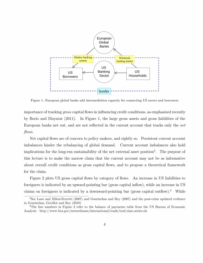
The broad picture that emerges of the role of European global banks in determining US
financial conditions can be depicted in terms of the schematic in Figure 1. European banks
draw wholesale funding from the United States and then lend it back to US residents. Al-
though European banks’ presence in the domestic US commercial banking sector is small, their
impact on overall credit conditions looms much larger through the shadow banking system in
the United States that relies on capital market-based financial intermediaries who intermediate
funds through securitization of claims.
The role of European global banks in determining US financial conditions highlights the
1The impact of global liquidity on emerging and developing economies has been explored in Bruno and Shin
(2011).2See, for instance, the BIS studies by Baba, McCauley and Ramaswamy (2009) and McGuire and von Peter
(2009) on the use of US dollar wholesale funding by European global banks. Acharya and Schnabl (2009) report
that European banks were sponsors for around 70% of the asset-backed commercial paper (ABCP) originated
prior to the subprime crisis.
3
US Households
USBorrowers
US Banking Sector
EuropeanGlobal Banks
border
Wholesalefunding market
Shadow bankingsystem
Figure 1. European global banks add intermediation capacity for connecting US savers and borrowers
importance of tracking gross capital flows in influencing credit conditions, as emphasized recently
by Borio and Disyatat (2011). In Figure 1, the large gross assets and gross liabilities of the
European banks net out, and are not reflected in the current account that tracks only the net
flows.
Net capital flows are of concern to policy makers, and rightly so. Persistent current account
imbalances hinder the rebalancing of global demand. Current account imbalances also hold
implications for the long-run sustainability of the net external asset position3. The purpose of
this lecture is to make the narrow claim that the current account may not be as informative
about overall credit conditions as gross capital flows, and to propose a theoretical framework
for the claim.
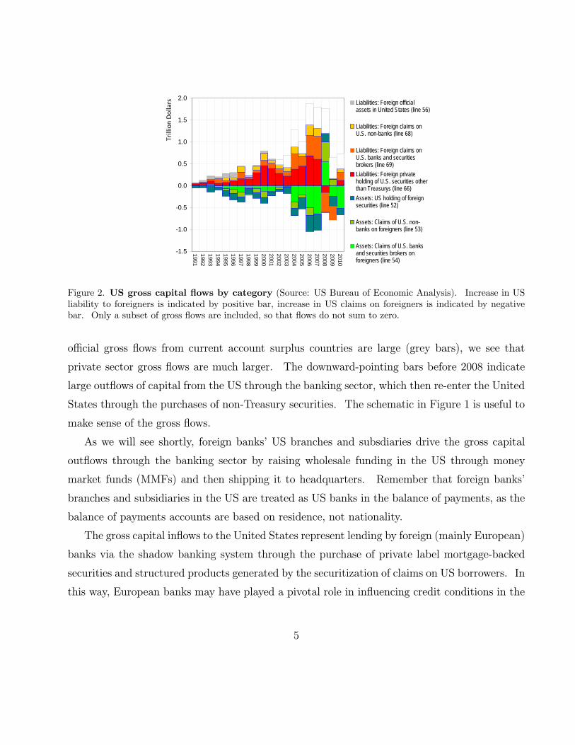
Figure 2 plots US gross capital flows by category of flows. An increase in US liabilities to
foreigners is indicated by an upward-pointing bar (gross capital inflow), while an increase in US
claims on foreigners is indicated by a downward-pointing bar (gross capital outflow).4 While
3See Lane and Milesi-Ferretti (2007) and Gourinchas and Rey (2007) and the post-crisis updated evidence
in Gourinchas, Govillot and Rey (2010)4The line numbers in Figure 2 refer to the balance of payments table from the US Bureau of Economic
Analysis: http://www.bea.gov/newsreleases/international/trade/trad time series.xls
4
-1.5
-1.0
-0.5
0.0
0.5
1.0
1.5
2.0
19
91
19
92
19
93
19
94
19
95
19
96
19
97
19
98
19
99
20
00
20
01
20
02
20
03
20
04
20
05
20
06
20
07
20
08
20
09
20
10
Trillion Dollars Liabilities: Foreign official
assets in United States (line 56)
Liabilities: Foreign claims onU.S. non-banks (line 68)
Liabilities: Foreign claims onU.S. banks and securitiesbrokers (line 69)
Liabilities: Foreign privateholding of U.S. securities otherthan Treasurys (line 66)
Assets: US holding of foreignsecurities (line 52)
Assets: Claims of U.S. non-banks on foreigners (line 53)
Assets: Claims of U.S. banksand securities brokers onforeigners (line 54)
Figure 2. US gross capital flows by category (Source: US Bureau of Economic Analysis). Increase in US
liability to foreigners is indicated by positive bar, increase in US claims on foreigners is indicated by negative
bar. Only a subset of gross flows are included, so that flows do not sum to zero.
official gross flows from current account surplus countries are large (grey bars), we see that
private sector gross flows are much larger. The downward-pointing bars before 2008 indicate
large outflows of capital from the US through the banking sector, which then re-enter the United
States through the purchases of non-Treasury securities. The schematic in Figure 1 is useful to
make sense of the gross flows.
As we will see shortly, foreign banks’ US branches and subsdiaries drive the gross capital
outflows through the banking sector by raising wholesale funding in the US through money
market funds (MMFs) and then shipping it to headquarters. Remember that foreign banks’
branches and subsidiaries in the US are treated as US banks in the balance of payments, as the
balance of payments accounts are based on residence, not nationality.
The gross capital inflows to the United States represent lending by foreign (mainly European)
banks via the shadow banking system through the purchase of private label mortgage-backed
securities and structured products generated by the securitization of claims on US borrowers. In
this way, European banks may have played a pivotal role in influencing credit conditions in the
5
United States by providing US dollar intermediation capacity. However, since the eurozone has
a roughly balanced current account while the UK is actually a deficit country, their collective
net capital flows vis-a-vis the United States do not reflect the influence of their banks in setting
overall credit conditions in the US. The distinction between net and gross flows is a classic
theme in international finance5, but deserves renewed attention given the new patterns of gross
capital flows due to global banking.
This lecture comes in two parts. In the first part, I will piece together the evidence from
the global flow of funds in drawing out the main hypothesis. The evidence comes from the BIS
banking statistics, which is supplemented with other aggregate data from previous studies and
the Federal Reserve’s Flow of Funds data for the United States.
The second part of the lecture develops a theoretical model of the impact of global banking
on US domestic credit conditions. The credit supply component of the model is the flip side
of a credit risk model where lending expands to fill up any spare balance sheet capacity when
measured risks are low. The balance sheet constraint binds all the time, so that in periods of
low measured risks, balance sheets must be large enough so that the risk constraint binds in
spite of the low measured risks.
In formulating the model of credit supply as the flip side of a credit risk model, the approach
rests on the corporate finance of bank balance sheet management. In textbook discussions of
corporate financing decisions, the set of positive net present value (NPV) projects is often taken
as being exogenously given, with the implication that the size of the balance sheet is fixed.
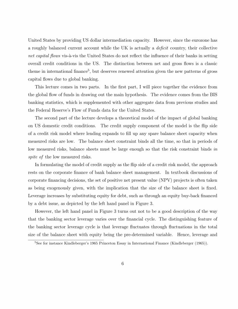
Leverage increases by substituting equity for debt, such as through an equity buy-back financed
by a debt issue, as depicted by the left hand panel in Figure 3.
However, the left hand panel in Figure 3 turns out not to be a good description of the way
that the banking sector leverage varies over the financial cycle. The distinguishing feature of
the banking sector leverage cycle is that leverage fluctuates through fluctuations in the total
size of the balance sheet with equity being the pre-determined variable. Hence, leverage and
5See for instance Kindleberger’s 1965 Princeton Essay in International Finance (Kindleberger (1965)).
6
A L
AssetsEquity
Debt
A L
Assets
Equity
Debt
A L
Assets
Equity
Debt
A L
Assets
Equity
Debt
Mode 1: Increased leverage with assets fixed Mode 2: Increased leverage via asset growth
Figure 3. Two Modes of Leveraging Up. In the left panel, the firm keeps assets fixed but replaces equity
with debt. In the right panel, the firm keeps equity fixed and increases the size of its balance sheet.
total assets tend to move in lock-step, as depicted in the right hand panel of Figure 3.6
Banks and other financial intermediaries’ lending depends on their “balance sheet capacity”.
Balance sheet capacity, in turn, depends on two things — the amount of bank capital and the
degree of “permitted leverage” as implied by the credit risk of the bank’s portfolio and the
amount of capital that the bank keeps to meet that credit risk. Bank lending expands to fill
up any spare balance sheet capacity when measured risks are low. Since the balance sheet
constraint binds all the time, lending expands in tranquil times in order that the risk constraint
binds in spite of the low measured risks. Borio and Disyatat (2011) have coined the term
“excess elasticity” to describe the tendency of the banking system to expand when financial
constraints are relaxed.
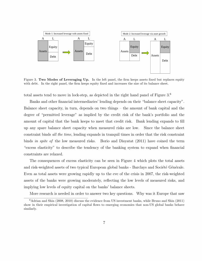
The consequences of excess elasticity can be seen in Figure 4 which plots the total assets
and risk-weighted assets of two typical European global banks - Barclays and Societe Generale.
Even as total assets were growing rapidly up to the eve of the crisis in 2007, the risk-weighted
assets of the banks were growing moderately, reflecting the low levels of measured risks, and
implying low levels of equity capital on the banks’ balance sheets.
More research is needed in order to answer two key questions. Why was it Europe that saw
6Adrian and Shin (2008, 2010) discuss the evidence from US investment banks, while Bruno and Shin (2011)
show in their empirical investigation of capital flows to emerging economies that non-US global banks behave
similarly.
7

0.0
0.2
0.4
0.6
0.8
1.0
1.2
1.4
1992
1993
1994
1995
1996
1997
1998
1999
2000
2001
2002
2003
2004
2005
2006
2007
Tri
llion
pou
nds
Total Assets
Risk-WeightedAssets
Barclays (1992 – 2007) Société Générale (1999 – 2007)
0.0
0.2
0.4
0.6
0.8
1.0
1.2
1999
2000
2001
2002
2003
2004
2005
2006
2007
Tri
llion
Eur
os
Total Assets
Risk-WeightedAssets
Figure 4. Total assets and risk-weighted assets of Barclays and Societe Generale (Source: Bankscope)
such rapid increases in banking capacity, and why did European (and not US) banks expand
intermediation between US borrowers and savers? Two likely elements of the answer to both
questions is the regulatory environment in Europe and the advent of the euro. The European
Union was the jurisdiction that embraced the spirit of the Basel II regulations most enthusias-
tically, while the rapid growth of cross-border banking within the eurozone after the advent of
the euro in 1999 provided fertile conditions for rapid growth of the European banking sector.
The permissive bank risk management practices epitomized in the Basel II proposals were
already widely practised within Europe as banks became more adept at circumventing the spirit
of the initial 1988 Basel I Accord. Basel II was subsequently codified most thoroughly in
the European Union through the EU’s Capital Adequacy Directive (CAD).7 In contrast, US
regulators have been more ambivalent toward Basel II, and chose to maintain relatively more
stringent regulations (at least, in the formal regulated banking sector) such as the cap on bank
leverage.
In order to emphasize the link between the expansion of global banking and the risk man-
agement practices embodied in the Basel II regulations, the key element of the theoretical model
7See Danielsson et al. (2001) for an early comment on the potential adverse impact of Basel II for financial
stability. See also Shin (2010, chapter 10) for historical background.
8
employed in this lecture will be the Vasicek (2002) credit risk model, which has served as the
backbone of the Basel capital rules.
The central message of this lecture is that the current account may not be as informative
about overall credit conditions as gross capital flows, especially gross capital flows generated by
the banking sector. If the claim is correct, then there are two important implications, one for
policy makers and one for researchers. Policy makers on their guard against the build-up of
financial vulnerabilities cannot rely merely on monitoring the current account. Researchers, for
their part, must take the financial system seriously when addressing overall financial conditions,
rather than seeing the financial sector as just the residual of the real side of the economy. In
this respect, researchers would do well to retrace the motivation for the work of Fleming (1962)
and Mundell (1963), who elevated capital flows as a topic worthy of study in its own right. We
will review some of the specific methodological lessons at the end of the lecture.
The outline of the lecture is as follows. I begin in the next section by taking stock of the
evidence from the BIS banking statistics on the global flow of funds. Section 3 presents the
formal model of direct and intermediated credit where the main implications of the impact of
global banks on credit conditions are derived as consequences. The paper concludes with some
observations on the origin of the European banking crisis of 2011 and the likely impact of the
European crisis on global financial stability.
2 Global Flow of Funds Perspective
Let us begin by examining the evidence for the role of global banks in determining US financial
conditions. We will take a “flow of funds” approach by tracking gross flows in the economy,
but from a global perspective. As stated at the outset, the two themes that emerge from the
investigation is the role of European global banks as the protagonists in the transmission of global
liquidity and the US Dollar as the currency underpinning the global banking system. Taken
together, the two elements imply a pivotal role for European banks in determining financial
conditions in the United States.
9
-12.0
-10.0
-8.0
-6.0
-4.0
-2.0
0.0
2.0
4.0
6.0
8.0
10.0
12.0
Mar.1999
Dec.1999
Sep.2000
Jun.2001
Mar.2002
Dec.2002
Sep.2003
Jun.2004
Mar.2005
Dec.2005
Sep.2006
Jun.2007
Mar.2008
Dec.2008
Sep.2009
Jun.2010
Tril
lion
Dol
lars U.S. dollar assets of
banks outside US
Euro assets of banksoutside eurozone
Sterling assets ofbanks outside UK
Yen assets of banksoutside Japan
Yen liabilities of banksoutside Japan
Sterling liabilities ofbanks outside UK
Euro liabilities of banksoutside eurozone
U.S. dollar liabilities ofbanks outside US
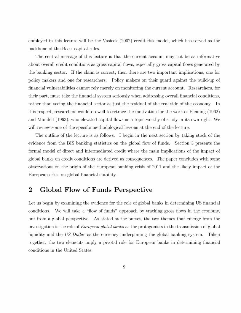
Figure 5. Cross-border foreign currency assets and liabilities of BIS reporting banks by currency (Source: BIS
locational banking statistics, Table 5A)
Much of our evidence comes from the banking statistics of the Bank for International Settle-
ments (BIS), and so some preliminary remarks are in order on how to read the numbers.8 The
BIS data come in two forms. First is the locational banking statistics, which are based on the
principle of residence, and which are consistent with the residency principle underlying balance
of payments and national income statistics. Under the locational statistics, the branches and
subsidiaries of the global banks are classified together with the host country banks.
The second type of data from the BIS are the consoldiated statistics, based on the nationality
of the parent bank. Within the consolidated banking statistics, foreign claims include the local
claims of branches and subsidiaries, while the international claims exclude local claims in local
(i.e. host country) currency.
Figure 5 is from the BIS locational banking statistics, and plots the total cross-border assets
and liabilities in foreign currency, classified according to currency. The top plot represents
the US dollar-denominated assets of BIS-reporting banks in foreign currency, and hence gives
the US dollar assets of banks outside the United States. The bottom plot in Figure 5 gives
8See BIS (2009) for details on the BIS banking statistics. See McGuire and von Peter (2009) for an example
of how the BIS statistics can be used in combination to reconstruct aggregate cross-border banking positions.
10
2008Q1
2.0
3.0
4.0
5.0
6.0
7.0
8.0
9.0
10.0
11.0
1999Q1
2000Q2
2001Q3
2002Q4
2004Q1
2005Q2
2006Q3
2007Q4
2009Q1
2010Q2
TrillionDollars
US charteredcommercialbanks' totalfinancialassets
US dollarassets ofbanks outsideUS
Figure 6. US dollar cross-border foreign currency claims and US commercial bank total assets (Source: Flow of
Funds, Federal Reserve and BIS locational banking statistics, Table 5A)
the corresponding US dollar-denominated liabilities of banks outside the United States. It is
immediately clear from the Figure that the US dollar plays a much more prominent role in
cross-border banking than does the euro, sterling or yen.
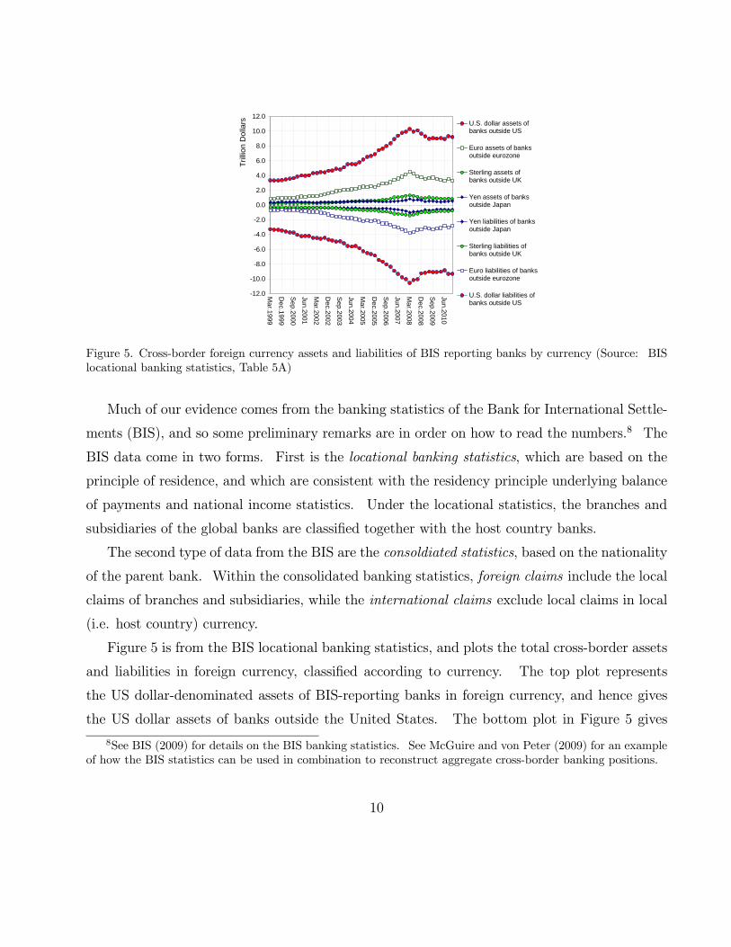
To gain some perspective on the size of the US dollar assets in Figure 5, we can plot the
total assets series next to the aggregate commercial banking sector in the United States, which
is given in Figure 6. We see that US dollar assets of banks outside the US exceeded $10 trillion
in 2008Q1, and briefly overtook the US chartered commercial banking sector in terms of total
assets. So, the sums are substantial. It is as if an offshore banking sector of comparable size
to the US commercial banking sector is intermediating US dollar claims and obligations.
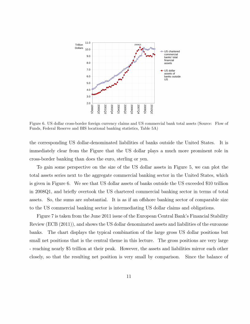
Figure 7 is taken from the June 2011 issue of the European Central Bank’s Financial Stability
Review (ECB (2011)), and shows the US dollar denominated assets and liabilities of the eurozone
banks. The chart displays the typical combination of the large gross US dollar positions but
small net positions that is the central theme in this lecture. The gross positions are very large
- reaching nearly $5 trillion at their peak. However, the assets and liabilities mirror each other
closely, so that the resulting net position is very small by comparison. Since the balance of
11
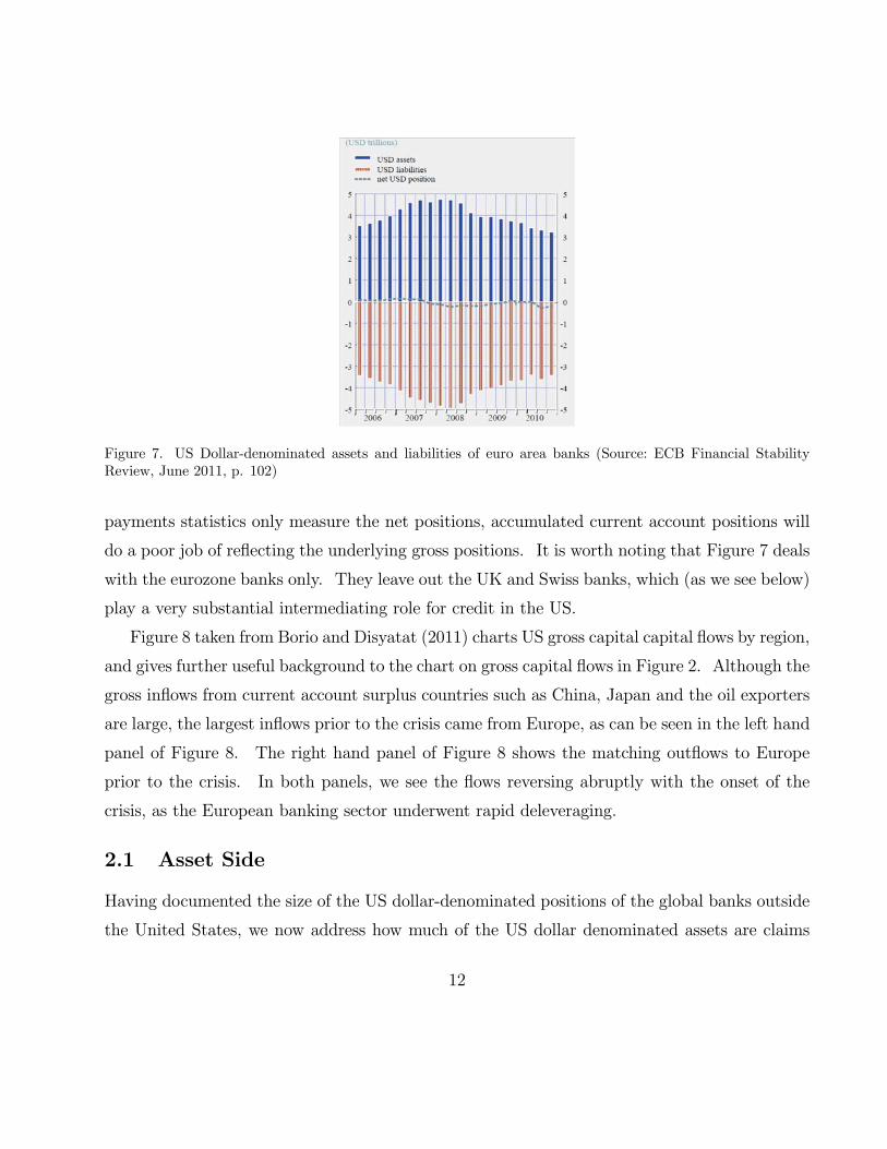
Figure 7. US Dollar-denominated assets and liabilities of euro area banks (Source: ECB Financial Stability
Review, June 2011, p. 102)
payments statistics only measure the net positions, accumulated current account positions will
do a poor job of reflecting the underlying gross positions. It is worth noting that Figure 7 deals
with the eurozone banks only. They leave out the UK and Swiss banks, which (as we see below)
play a very substantial intermediating role for credit in the US.
Figure 8 taken from Borio and Disyatat (2011) charts US gross capital capital flows by region,
and gives further useful background to the chart on gross capital flows in Figure 2. Although the
gross inflows from current account surplus countries such as China, Japan and the oil exporters
are large, the largest inflows prior to the crisis came from Europe, as can be seen in the left hand
panel of Figure 8. The right hand panel of Figure 8 shows the matching outflows to Europe
prior to the crisis. In both panels, we see the flows reversing abruptly with the onset of the
crisis, as the European banking sector underwent rapid deleveraging.
2.1 Asset Side
Having documented the size of the US dollar-denominated positions of the global banks outside
the United States, we now address how much of the US dollar denominated assets are claims
12
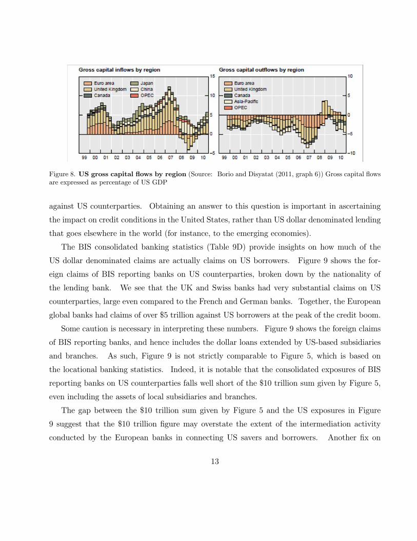
Figure 8. US gross capital flows by region (Source: Borio and Disyatat (2011, graph 6)) Gross capital flows
are expressed as percentage of US GDP
against US counterparties. Obtaining an answer to this question is important in ascertaining
the impact on credit conditions in the United States, rather than US dollar denominated lending
that goes elsewhere in the world (for instance, to the emerging economies).
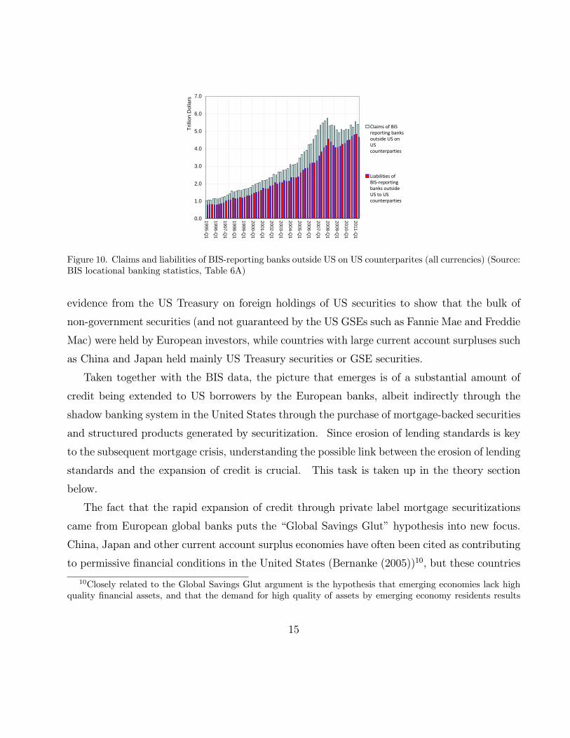
The BIS consolidated banking statistics (Table 9D) provide insights on how much of the
US dollar denominated claims are actually claims on US borrowers. Figure 9 shows the for-
eign claims of BIS reporting banks on US counterparties, broken down by the nationality of
the lending bank. We see that the UK and Swiss banks had very substantial claims on US
counterparties, large even compared to the French and German banks. Together, the European
global banks had claims of over $5 trillion against US borrowers at the peak of the credit boom.
Some caution is necessary in interpreting these numbers. Figure 9 shows the foreign claims
of BIS reporting banks, and hence includes the dollar loans extended by US-based subsidiaries
and branches. As such, Figure 9 is not strictly comparable to Figure 5, which is based on
the locational banking statistics. Indeed, it is notable that the consolidated exposures of BIS
reporting banks on US counterparties falls well short of the $10 trillion sum given by Figure 5,
even including the assets of local subsidiaries and branches.
The gap between the $10 trillion sum given by Figure 5 and the US exposures in Figure
9 suggest that the $10 trillion figure may overstate the extent of the intermediation activity
conducted by the European banks in connecting US savers and borrowers. Another fix on
13

0.0
1.0
2.0
3.0
4.0
5.0
6.0
7.0
2005-Q2
2005-Q4
2006-Q2
2006-Q4
2007-Q2
2007-Q4
2008-Q2
2008-Q4
2009-Q2
2009-Q4
2010-Q2
2010-Q4
Trillion Dollars
Non-European BISreporting countries
Other European BISreporting countries
Switzerland
United Kingdom
France
Germany
Figure 9. Foreign claims of BIS reporting banks on US counterparties (Source: BIS consolidated banking
statistics, Table 9D)
how much of the $10 trillion is with US counterparties is given in Figure 10 from the BIS
locational statistics (Table 6A) that shows the claims and liabilities of banks outside the US on
US counterparties. Even though this series includes claims in all currencies, the series peaks
at $5.73 trillion,9 leaving a big gap compared to the $10 trillion figure. Part of the remainder
of the $10 trillion sum may be accounted for by lending to emerging economies, but another
possibility (perhaps more plausible) is that the $10 trillion sum incorporates substantial double-
counting of US dollar exposures that are held between global banks. Yet another possibility is
that the holdings of offshore financial centers account for part of the gap. More disaggregated
data would help to resolve these questions. What is clear is that a very substantial portion of
the $10 trillion dollar-denominated assets do not involve directly a US counterparty, highlighting
the importance of the US dollar as the currency that underpins the global banking system.
Although the BIS banking statistics do not provide a detailed breakdown by the type of
asset held by the bank, data on holdings of US securities suggest that a substantial portion of
the claims of European banks were US private label securities. Milesi-Ferretti (2009) draws on
9The US dollar only series peaks at $4.8 trillion in 2008Q1, of which $1 trillion is the claim held by branches
of US banks on their parent. I am grateful to Carol Bertaut for pointing this out.
14
0.0
1.0
2.0
3.0
4.0
5.0
6.0
7.0
19
95
-Q1
19
96
-Q1
19
97
-Q1
19
98
-Q1
19
99
-Q1
20
00
-Q1
20
01
-Q1
20
02
-Q1
20
03
-Q1
20
04
-Q1
20
05
-Q1
20
06
-Q1
20
07
-Q1
20
08
-Q1
20
09
-Q1
20
10
-Q1
20
11
-Q1
Tril
lion
Do
llars
Claims of BISreporting banksoutside US onUScounterparties
Liabilities ofBIS‐reportingbanks outsideUS to UScounterparties
Figure 10. Claims and liabilities of BIS-reporting banks outside US on US counterparites (all currencies) (Source:
BIS locational banking statistics, Table 6A)
evidence from the US Treasury on foreign holdings of US securities to show that the bulk of
non-government securities (and not guaranteed by the US GSEs such as Fannie Mae and Freddie
Mac) were held by European investors, while countries with large current account surpluses such
as China and Japan held mainly US Treasury securities or GSE securities.
Taken together with the BIS data, the picture that emerges is of a substantial amount of
credit being extended to US borrowers by the European banks, albeit indirectly through the
shadow banking system in the United States through the purchase of mortgage-backed securities
and structured products generated by securitization. Since erosion of lending standards is key
to the subsequent mortgage crisis, understanding the possible link between the erosion of lending
standards and the expansion of credit is crucial. This task is taken up in the theory section
below.
The fact that the rapid expansion of credit through private label mortgage securitizations
came from European global banks puts the “Global Savings Glut” hypothesis into new focus.
China, Japan and other current account surplus economies have often been cited as contributing
to permissive financial conditions in the United States (Bernanke (2005))10, but these countries
10Closely related to the Global Savings Glut argument is the hypothesis that emerging economies lack high
quality financial assets, and that the demand for high quality of assets by emerging economy residents results
15
held mainly Treasury and GSE securities rather than the private label securities that provided
financing for subprime mortages. Although GSEs channeled funding to the US housing market
also, subprime lending was securitized mainly through private label (i.e. non-GSE) securitiza-
tions. Of the non-US intermediaries, it was the European banks that were exposed most to the
securities and structured products associated with subprime.
More recently, Bernanke, Bertaut, DeMarco, and Kamin (2011) and Bertaut, DeMarco,
Kamin and Tryon (2011) have drawn attention to capital flows emanating from European in-
vestors, pointing to the need to modify the original Global Savings Glut hypothesis. They also
consider a mechanism whereby the current account surplus countries had an indirect impact
on US credit conditions by pushing down long-term yields on US Treasury securities, thereby
inducing a substitution away from Treasury securities into private label securities by European
investors - a type of “crowding out” effect. However, such an account sits uncomfortably with
the evidence from Figure 9 that European global banks raised their assets in the US, increas-
ing their claims against US borrowers by close to 40% from 2005 to 2007, rather than merely
substituting their holdings away from Treasuries into private label securities.
Further work may uncover the extent to which the current account surplus countries drove
European banks into private label securities, but a more plausible mechanism for the expansion
of European banks’ assets against US borrowers appears to be the increase in the overall size
of their balance sheets driven by lower measured risks and increased balance sheet capacity.
Rather than the “Global Savings Glut”, it seems more plausible to attribute the lowering of
credit standards prior to the subprime crisis to the “Global Banking Glut” generated by the
overcapacity in the banking sector. We derive a formal model of the Global Banking Glut in
our theory section below.
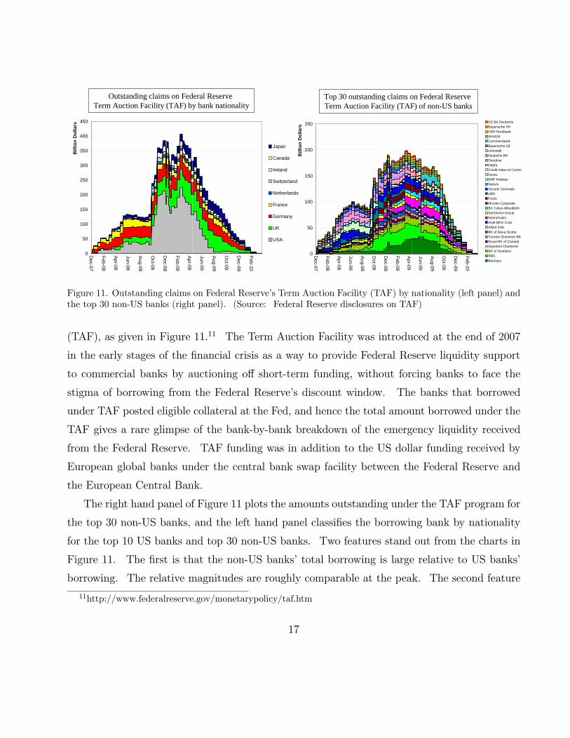
Another snapshot of the asset side of the European global banks is from the Federal Reserve’s
disclosures on the liquidity support given to commercial banks under the Term Auction Facility
in current account imbalances and lower interest rates in the United States. See, for instance, Caballero, Fahri
and Gourinchas (2008).
16
0
50
100
150
200
250
300
350
400
450
Dec-07
Feb-08
Apr-08
Jun-08
Aug-08
Oct-08
Dec-08
Feb-09
Apr-09
Jun-09
Aug-09
Oct-09
Dec-09
Feb-10
Bill
ion
Do
llars
Japan
Canada
Ireland
Switzerland
Netherlands
France
Germany
UK
USA
0
50
100
150
200
250
Dec-07
Feb-08
Apr-08
Jun-08
Aug-08
Oct-08
Dec-08
Feb-09
Apr-09
Jun-09
Aug-09
Oct-09
Dec-09
Feb-10
Bil
lio
n D
oll
ars
DZ BK DeutscheBayerische HV
HSH NordbankWestLBCommerzbank
Bayerische LBUnicreditDeutsche BK
DresdnerDepfaCredit Indus et Comm
DexiaBNP ParibasNatixis
Societe GeneraleUBSFortis
Mizuho CorporateBK Tokyo-MitsubishiSumitomo Group
NorinchukinArab BKG CorpAllied Irish
BK of Nova ScotiaToronto Dominion BKRoyal BK of Canada
Standard CharteredBK of ScotlandRBS
Barclays
Outstanding claims on Federal Reserve Term Auction Facility (TAF) by bank nationality
Top 30 outstanding claims on Federal Reserve Term Auction Facility (TAF) of non-US banks
Figure 11. Outstanding claims on Federal Reserve’s Term Auction Facility (TAF) by nationality (left panel) and
the top 30 non-US banks (right panel). (Source: Federal Reserve disclosures on TAF)
(TAF), as given in Figure 11.11 The Term Auction Facility was introduced at the end of 2007
in the early stages of the financial crisis as a way to provide Federal Reserve liquidity support
to commercial banks by auctioning off short-term funding, without forcing banks to face the
stigma of borrowing from the Federal Reserve’s discount window. The banks that borrowed
under TAF posted eligible collateral at the Fed, and hence the total amount borrowed under the
TAF gives a rare glimpse of the bank-by-bank breakdown of the emergency liquidity received
from the Federal Reserve. TAF funding was in addition to the US dollar funding received by
European global banks under the central bank swap facility between the Federal Reserve and
the European Central Bank.
The right hand panel of Figure 11 plots the amounts outstanding under the TAF program for
the top 30 non-US banks, and the left hand panel classifies the borrowing bank by nationality
for the top 10 US banks and top 30 non-US banks. Two features stand out from the charts in
Figure 11. The first is that the non-US banks’ total borrowing is large relative to US banks’
borrowing. The relative magnitudes are roughly comparable at the peak. The second feature
11http://www.federalreserve.gov/monetarypolicy/taf.htm
17
that stands out is the preponderance of European banks in the list of non-US recipients of TAF
funding. The UK banks are especially prominent, led by Barclays, RBS and Bank of Scotland.
The list also reveals some unlikely names, such as Norinchukin (the Agricultural Savings Bank
of Japan) and the German landesbanks, who are likely to have ventured into US dollar lending
in their search for higher yielding assets to deploy their large domestic deposit bases.
2.2 Liabilities Side
We now turn to the liabilities side of the European global banks’ balance sheet in the schematic
of Figure 1, and examine the evidence on how they raised US dollar funding. A recent BIS
(2010) study notes that as of September 2009, the United States hosted the branches of 161
foreign banks who collectively raised over $1 trillion dollars’ worth of wholesale bank funding,
of which $645 billion was channeled for use by their headquarters. Money market funds in the
United States are an important source of wholesale bank funding for global banks.
Even in net terms, foreign banks have been channeling large amounts of dollar funding to
head office. That is, the funding channeled to head office is much larger than the funding
received by the branch from head office. The BIS (2010) study finds that foreign bank branches
had a net positive interoffice position in September 2009 amounting to $468 billion vis-a-vis
their headquarters.
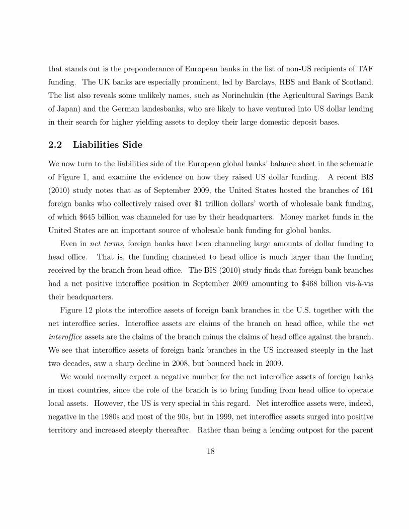
Figure 12 plots the interoffice assets of foreign bank branches in the U.S. together with the
net interoffice series. Interoffice assets are claims of the branch on head office, while the net
interoffice assets are the claims of the branch minus the claims of head office against the branch.
We see that interoffice assets of foreign bank branches in the US increased steeply in the last
two decades, saw a sharp decline in 2008, but bounced back in 2009.
We would normally expect a negative number for the net interoffice assets of foreign banks
in most countries, since the role of the branch is to bring funding from head office to operate
local assets. However, the US is very special in this regard. Net interoffice assets were, indeed,
negative in the 1980s and most of the 90s, but in 1999, net interoffice assets surged into positive
territory and increased steeply thereafter. Rather than being a lending outpost for the parent
18
31-Dec-08
30-Jun-08
-100
0
100
200
300
400
500
600
700
800
900
Mar-85
Sep-86
Mar-88
Sep-89
Mar-91
Sep-92
Mar-94
Sep-95
Mar-97
Sep-98
Mar-00
Sep-01
Mar-03
Sep-04
Mar-06
Sep-07
Mar-09
Sep-10
Bil
lio
n D
oll
ars
Interoffice Assets of ForeignBanks in US
Net Interoffice Assets ofForeign Banks in US
Figure 12. Interoffice assets of foreign bank in the United States (Source: Federal Reserve, series on “Assets and
Liabilities of U.S. Branches and Agencies of Foreign Banks”)
bank, the US branches became a funding source for the parent.
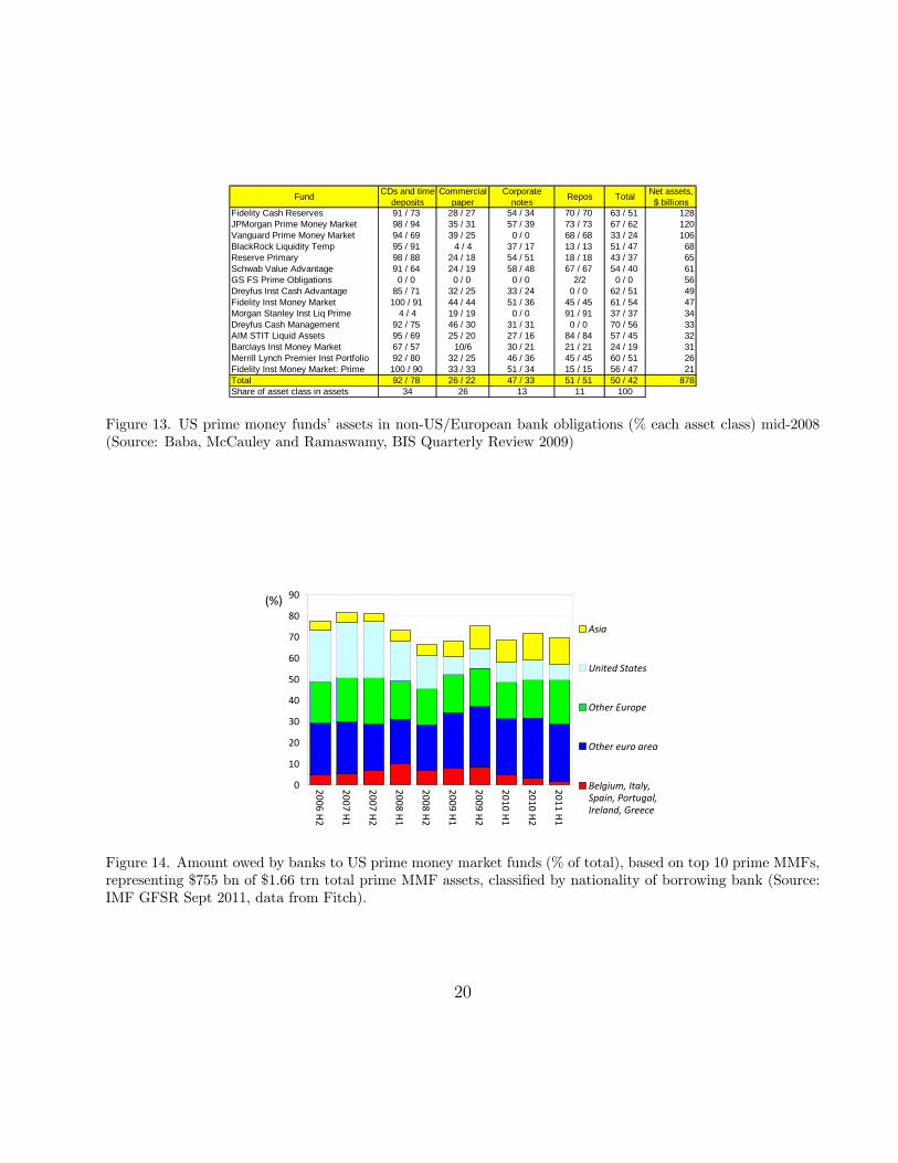
Figure 13 reproduces the table from Baba, McCauley and Ramaswamy (2009) which provides
a snapshot of the way that European banks obtained dollar funding on the eve of the 2008
Lehman crisis. By mid-2008, 50% of the assets of U.S. prime money market funds were short-
term obligations of foreign banks, with the lion’s share owed by European banks.
Figure 14, taken from the recent issue of the IMF’s Global Financial Stability Report, plots
the time series of the amount owed by banks to US prime money market funds expressed as a
percentage of the total assets of the 10 largest prime money market funds, representing $755
billion of the $1.66 trillion total prime MMF assets in June 2011. We see the preponderance
of bank obligations as the primary asset class of the prime money market funds, especially the
obligations of European banks. We see from this chart that, in essence, the US prime money
market funds serve as the base of the shadow banking system in the United States, playing a
comparable role to customer deposits in the regulated banking sector. The difference is that
the intermediation chain in the shadow banking sector can be much longer and multi-layered,
involved many categories of financial intermediaries.
19
Fund CDs and time
deposits Commercial
paper Corporate
notesRepos Total
Net assets, $ billions
Fidelity Cash Reserves 91 / 73 28 / 27 54 / 34 70 / 70 63 / 51 128JPMorgan Prime Money Market 98 / 94 35 / 31 57 / 39 73 / 73 67 / 62 120Vanguard Prime Money Market 94 / 69 39 / 25 0 / 0 68 / 68 33 / 24 106BlackRock Liquidity Temp 95 / 91 4 / 4 37 / 17 13 / 13 51 / 47 68Reserve Primary 98 / 88 24 / 18 54 / 51 18 / 18 43 / 37 65Schwab Value Advantage 91 / 64 24 / 19 58 / 48 67 / 67 54 / 40 61GS FS Prime Obligations 0 / 0 0 / 0 0 / 0 2/2 0 / 0 56Dreyfus Inst Cash Advantage 85 / 71 32 / 25 33 / 24 0 / 0 62 / 51 49Fidelity Inst Money Market 100 / 91 44 / 44 51 / 36 45 / 45 61 / 54 47Morgan Stanley Inst Liq Prime 4 / 4 19 / 19 0 / 0 91 / 91 37 / 37 34Dreyfus Cash Management 92 / 75 46 / 30 31 / 31 0 / 0 70 / 56 33AIM STIT Liquid Assets 95 / 69 25 / 20 27 / 16 84 / 84 57 / 45 32Barclays Inst Money Market 67 / 57 10/6 30 / 21 21 / 21 24 / 19 31Merrill Lynch Premier Inst Portfolio 92 / 80 32 / 25 46 / 36 45 / 45 60 / 51 26Fidelity Inst Money Market: Prime 100 / 90 33 / 33 51 / 34 15 / 15 56 / 47 21Total 92 / 78 26 / 22 47 / 33 51 / 51 50 / 42 878Share of asset class in assets 34 26 13 11 100
Figure 13. US prime money funds’ assets in non-US/European bank obligations (% each asset class) mid-2008
(Source: Baba, McCauley and Ramaswamy, BIS Quarterly Review 2009)
0
10
20
30
40
50
60
70
80
90
2006 H2
2007 H1
2007 H2
2008 H1
2008 H2
2009 H1
2009 H2
2010 H1
2010 H2
2011 H1
(%)
Asia
United States
Other Europe
Other euro area
Belgium, Italy,Spain, Portugal,Ireland, Greece
Figure 14. Amount owed by banks to US prime money market funds (% of total), based on top 10 prime MMFs,
representing $755 bn of $1.66 trn total prime MMF assets, classified by nationality of borrowing bank (Source:
IMF GFSR Sept 2011, data from Fitch).
20
0
20
40
60
80
100
120
140
160
180
200
France
UK
Netherlands
Germ
ay
Sw
itzerland
Sw
eden
Norw
ay
Denm
ark
Italy
Spain
Austria
Belgium
Luxembourg
Bill
ion
Do
llars
Figure 15. Amounts owed by European banks to US prime money market funds, classified by nationality of
borrowing bank (end-June 2011) (Source: IMF GFSR September 2011, data from Fitch)
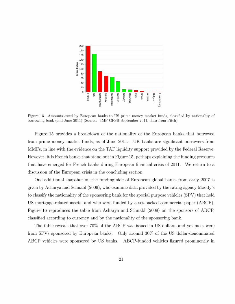
Figure 15 provides a breakdown of the nationality of the European banks that borrowed
from prime money market funds, as of June 2011. UK banks are significant borrowers from
MMFs, in line with the evidence on the TAF liquidity support provided by the Federal Reserve.
However, it is French banks that stand out in Figure 15, perhaps explaining the funding pressures
that have emerged for French banks during European financial crisis of 2011. We return to a
discussion of the European crisis in the concluding section.
One additional snapshot on the funding side of European global banks from early 2007 is
given by Acharya and Schnabl (2009), who examine data provided by the rating agency Moody’s
to classify the nationality of the sponsoring bank for the special purpose vehicles (SPV) that held
US mortgage-related assets, and who were funded by asset-backed commercial paper (ABCP).
Figure 16 reproduces the table from Acharya and Schnabl (2009) on the sponsors of ABCP,
classified according to currency and by the nationality of the sponsoring bank.
The table reveals that over 70% of the ABCP was issued in US dollars, and yet most were
from SPVs sponsored by European banks. Only around 30% of the US dollar-denominated
ABCP vehicles were sponsored by US banks. ABCP-funded vehicles figured prominently in
21
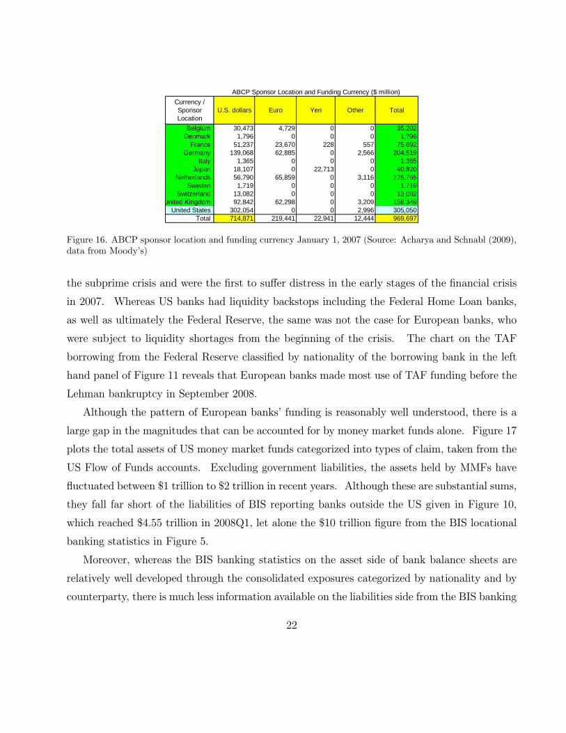
ABCP Sponsor Location and Funding Currency ($ million)
Currency / Sponsor Location
U.S. dollars Euro Yen Other Total
Belgium 30,473 4,729 0 0 35,202Denmark 1,796 0 0 0 1,796
France 51,237 23,670 228 557 75,692Germany 139,068 62,885 0 2,566 204,519
Italy 1,365 0 0 0 1,365Japan 18,107 0 22,713 0 40,820
Netherlands 56,790 65,859 0 3,116 125,765Sweden 1,719 0 0 0 1,719
Switzerland 13,082 0 0 0 13,082United Kingdom 92,842 62,298 0 3,209 158,349
United States 302,054 0 0 2,996 305,050Total 714,871 219,441 22,941 12,444 969,697
Figure 16. ABCP sponsor location and funding currency January 1, 2007 (Source: Acharya and Schnabl (2009),
data from Moody’s)
the subprime crisis and were the first to suffer distress in the early stages of the financial crisis
in 2007. Whereas US banks had liquidity backstops including the Federal Home Loan banks,
as well as ultimately the Federal Reserve, the same was not the case for European banks, who
were subject to liquidity shortages from the beginning of the crisis. The chart on the TAF
borrowing from the Federal Reserve classified by nationality of the borrowing bank in the left
hand panel of Figure 11 reveals that European banks made most use of TAF funding before the
Lehman bankruptcy in September 2008.
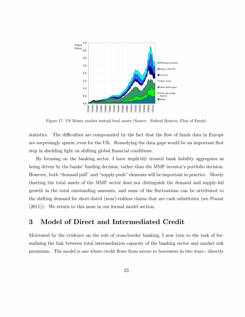
Although the pattern of European banks’ funding is reasonably well understood, there is a
large gap in the magnitudes that can be accounted for by money market funds alone. Figure 17
plots the total assets of US money market funds categorized into types of claim, taken from the
US Flow of Funds accounts. Excluding government liabilities, the assets held by MMFs have
fluctuated between $1 trillion to $2 trillion in recent years. Although these are substantial sums,
they fall far short of the liabilities of BIS reporting banks outside the US given in Figure 10,
which reached $4.55 trillion in 2008Q1, let alone the $10 trillion figure from the BIS locational
banking statistics in Figure 5.
Moreover, whereas the BIS banking statistics on the asset side of bank balance sheets are
relatively well developed through the consolidated exposures categorized by nationality and by
counterparty, there is much less information available on the liabilities side from the BIS banking
22
0.0
0.5
1.0
1.5
2.0
2.5
3.0
3.5
4.0
1980Q1
1982Q1
1984Q1
1986Q1
1988Q1
1990Q1
1992Q1
1994Q1
1996Q1
1998Q1
2000Q1
2002Q1
2004Q1
2006Q1
2008Q1
2010Q1
TrillionDollars
Municipal securities
Agency and GSE
Treasury
Other Assets
Open market paper
Time and savingsdeposits
Repos
Figure 17. US Money market mutual fund assets (Source: Federal Reserve, Flow of Funds)
statistics. The difficulties are compounded by the fact that the flow of funds data in Europe
are surprisingly sparse, even for the UK. Remedying the data gaps would be an important first
step in shedding light on shifting global financial conditions.
By focusing on the banking sector, I have implicitly treated bank liability aggregates as
being driven by the banks’ funding decision, rather than the MMF investor’s portfolio decision.
However, both “demand pull” and “supply push” elements will be important in practice. Merely
charting the total assets of the MMF sector does not distinguish the demand and supply-led
growth in the total outstanding amounts, and some of the fluctuations can be attributed to
the shifting demand for short-dated (near)-riskless claims that are cash substitutes (see Poszar
(2011)). We return to this issue in our formal model section.
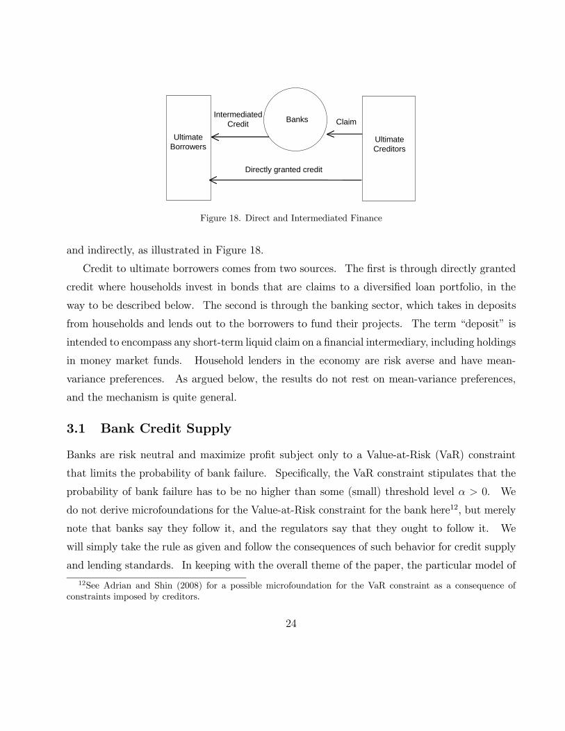
3 Model of Direct and Intermediated Credit
Motivated by the evidence on the role of cross-border banking, I now turn to the task of for-
malizing the link between total intermediation capacity of the banking sector and market risk
premiums. The model is one where credit flows from savers to borrowers in two ways - directly
23
Banks
UltimateCreditors
UltimateBorrowers
IntermediatedCredit Claim
Directly granted credit
Figure 18. Direct and Intermediated Finance
and indirectly, as illustrated in Figure 18.
Credit to ultimate borrowers comes from two sources. The first is through directly granted
credit where households invest in bonds that are claims to a diversified loan portfolio, in the
way to be described below. The second is through the banking sector, which takes in deposits
from households and lends out to the borrowers to fund their projects. The term “deposit” is
intended to encompass any short-term liquid claim on a financial intermediary, including holdings
in money market funds. Household lenders in the economy are risk averse and have mean-
variance preferences. As argued below, the results do not rest on mean-variance preferences,
and the mechanism is quite general.
3.1 Bank Credit Supply
Banks are risk neutral and maximize profit subject only to a Value-at-Risk (VaR) constraint
that limits the probability of bank failure. Specifically, the VaR constraint stipulates that the
probability of bank failure has to be no higher than some (small) threshold level 0. We
do not derive microfoundations for the Value-at-Risk constraint for the bank here12, but merely
note that banks say they follow it, and the regulators say that they ought to follow it. We
will simply take the rule as given and follow the consequences of such behavior for credit supply
and lending standards. In keeping with the overall theme of the paper, the particular model of
12See Adrian and Shin (2008) for a possible microfoundation for the VaR constraint as a consequence of
constraints imposed by creditors.
24
C
E
f1r1L
Bank
Figure 19. Notation for bank balance sheet. is the amount lent out at date 0, financed with equity and
deposits .
credit risk that drives the VaR constraint will be the one adopted by the Basel Committee for
Banking Supervision (BCBS (2005)).
Due to an aggregation result across banks to be shown below, it is without loss of generality
to consider the banking sector as being a single bank, encompassing domestic and global banks.
As long as all banks are subject to the same Value-at-Risk constraint, we may treat the whole
banking sector (domestic and global) to be one bank.
The notation to be used is given in Figure 19. The bank lends out amount (with “”
standing for “credit”) at date 0 at the lending rate , so that the bank is owed (1 + ) in
date 1 (its notional assets). The lending is financed from the combination of equity and
debt funding , where encompasses deposit and money market funding. The cost of debt
financing is so that the bank owes (1 + ) at date 1 (its notional liabilities).
The economy has a continuum of binary projects, each of which succeeds with probability
1 − and fails with probability . Each project uses debt financing of 1, which the borrower
will default on if the project fails. Thus, if the project fails, the lender suffers credit loss of 1.
The correlation in defaults across loans follows the Vasicek (2002) model, which has served as
the backbone of Basel capital requirements (Basel Committee on Banking Supervision (2005)).
Project succeeds (so that borrower repays the loan) when 0, where is the random
variable
= −Φ−1 () +√ +p1− (1)
where Φ () is the c.d.f. of the standard normal, and {} are independent standard normals,
25
and is a constant between zero and one. has the interpretation of the economy-wide
fundamental factor that affects all projects, while is the idiosyncratic factor for project .
The parameter is the weight on the common factor, which limits the extent of diversification
that investors can achieve. Note that the probability of default is given by
Pr ( 0) = Pr³√
+p1− Φ−1 ()
´= Φ
¡Φ−1 ()
¢= (2)
Banks are able to diversify their loan book by lending small amounts to a large number of
borrowers. Conditional on , defaults are independent. The bank can remove idiosyncratic
risk by keeping fixed but diversifying across borrowers - that is, by increasing number of
borrowers but reducing the face value of individual loans. In the limit, the realized value of
assets is function of only, by the law of large numbers. The realized value of the bank’s assets
at date 1 is given by the random variable ( ) where
( ) ≡ (1 + ) · Pr ( ≥ 0| )= (1 + ) · Pr
³√ +
p1− ≥ Φ−1 () |
´= (1 + ) · Φ
³√−Φ−1()√1−
´(3)
Then, the c.d.f. of ( ) is given by
() = Pr ( ≤ )
= Pr¡ ≤ −1 ()
¢= Φ
¡−1 ()
¢= Φ
µ1√
µΦ−1 () +
p1− Φ−1
µ
(1 + )
¶¶¶(4)
The density over the realized assets of the bank is the derivative of (4) with respect to .
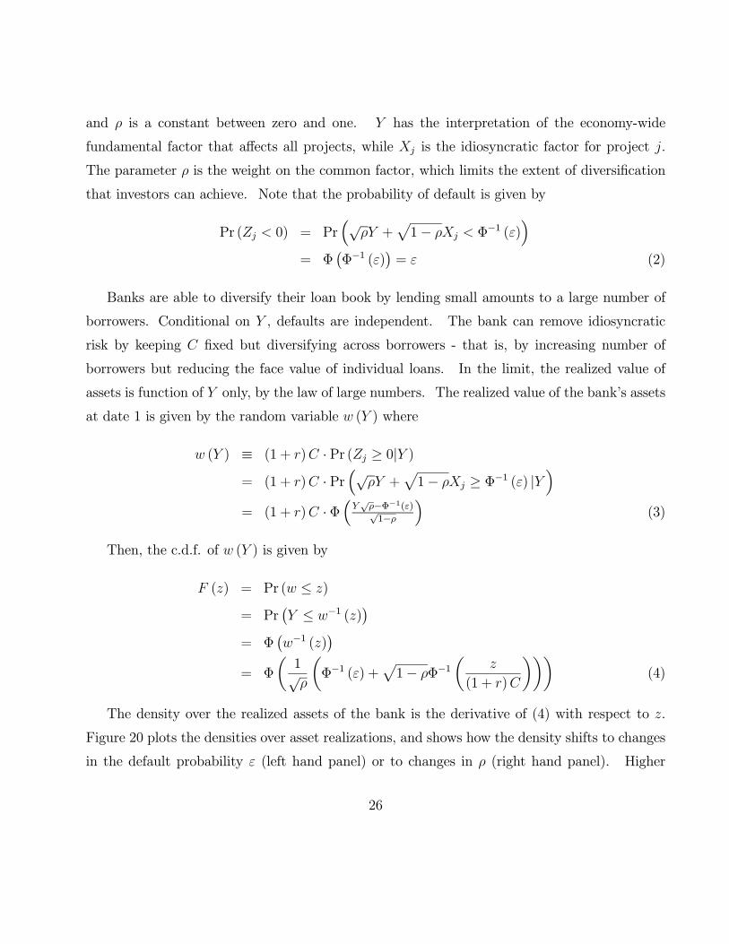
Figure 20 plots the densities over asset realizations, and shows how the density shifts to changes
in the default probability (left hand panel) or to changes in (right hand panel). Higher
26
0 0.2 0.4 0.6 0.8 10
2
4
6
8
10
12
z
dens
ity o
ver
real
ized
ass
ets
0 0.2 0.4 0.6 0.8 10
3
6
9
12
15
z
dens
ity o
ver
real
ized
ass
ets
ε = 0.2
ε = 0.3
ρ = 0.3 ε = 0.2
ε = 0.1
ρ = 0.01
ρ = 0.1
ρ = 0.3
Figure 20. The two charts plot the densities over realized assets when (1 + ) = 1. The left hand charts plots
the density over asset realizations of the bank when = 01 and is varied from 0.1 to 0.3. The right hand
chart plots the asset realization density when = 02 and varies from 0.01 to 0.3.
values of imply a first degree stochastic dominance shift left for the asset realization density,
while shifts in imply a mean-preserving shift in the density around the mean realization 1− .
The bank takes its equity as given and adjusts the size of its loan book and funding so
as as to keep its probability of default to 0.13 Since the bank is risk-neutral and maximizes
profit, the VaR constraint binds whenever expected profit to lending is positive. The constraint
is that the bank limits lending so as to keep the probability of its own failure to . Since
the bank fails when the asset realization falls below its notional liabilities (1 + ), the bank’s
credit supply satisfies
Pr ( (1 + )) = Φ
µΦ−1()+
√1−Φ−1( (1+)(1+) )√
¶= (5)
Re-arranging (5), we can derive an expression for the ratio of notional liabilities to notional
assets for the bank.
13See Adrian and Shin (2008, 2010) for empirical evidence that banks take equity as given and adjust leverage
by adjusting the size of their balance sheet.
27
Notional liabilities
Notional assets=(1 + )
(1 + )= Φ
µ√Φ−1 ()− Φ−1 ()√
1−
¶(6)
From here on, we will use the shorthand to denote this ratio of notional liabilities to
notational assets. That is,
( ) ≡ Φ³√
Φ−1()−Φ−1()√1−
´(7)
can be seen as a normalized leverage ratio, lying between zero and one. The higher is , the
higher is bank leverage and the greater is credit supply.
We can solve for bank credit supply and demand for deposit funding from (6) and the
balance sheet identity = + to give
=
1− 1+1+
· and =
1+
1+· 1− 1 (8)
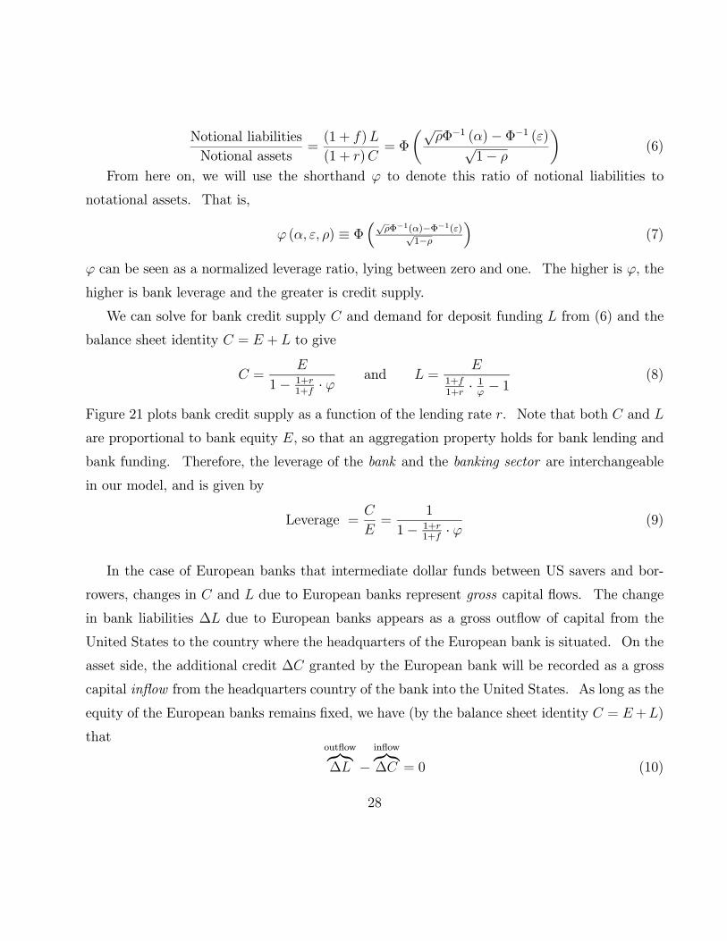
Figure 21 plots bank credit supply as a function of the lending rate . Note that both and
are proportional to bank equity , so that an aggregation property holds for bank lending and
bank funding. Therefore, the leverage of the bank and the banking sector are interchangeable
in our model, and is given by
Leverage =
=
1
1− 1+1+
· (9)
In the case of European banks that intermediate dollar funds between US savers and bor-
rowers, changes in and due to European banks represent gross capital flows. The change
in bank liabilities ∆ due to European banks appears as a gross outflow of capital from the
United States to the country where the headquarters of the European bank is situated. On the
asset side, the additional credit ∆ granted by the European bank will be recorded as a gross
capital inflow from the headquarters country of the bank into the United States. As long as the
equity of the European banks remains fixed, we have (by the balance sheet identity = +)
thatoutflowz}|{∆ −
inflowz}|{∆ = 0 (10)
28
0 f
E
111
1/
CreditSupply
11
f
rC
r
Figure 21. Bank credit supply curve
so that the net capital flow between the United States and the headquarters jurisdiction of the
European bank is zero, no matter how large are ∆ and ∆. Equation (10) can be interpreted
as the model counterpart to the schematic capital flow diagram of Figure 1 and the balance of
payments charts in Figures 2 and 8. Since the current account is a measure only the net flows
between countries, the impact of rapid growth in bank lending through the European banks will
not show up in the balance of payment statistics for the United States, potentially obscuring
the build-up of financial vulnerabilities from policy makers.
3.2 Credit Supply by Bond Investors
We now turn to the credit supply coming directly from households. Recall that households are
risk averse with mean-variance preferences. They have identical risk tolerance . Households
lend to borrowers by purchasing bonds that are claims on a diversified pool of loans that have
removed idiosyncratic credit risk so that the return densities are identical to those for the bank
loan book described above.
Households hold a portfolio consisting of three component assets - risky bonds, cash and
deposits in the bank. As stated already, deposits include claims on money market funds that
29
0 0.2 0.4 0.6 0.8 1.00
0.1
0.2
0.3
0.4
0.5
0.6
0.7
0.8
0.9
1.0Normalized leverage
default probability ε
norm
aliz
ed le
vera
ge φ
0 0.2 0.4 0.6 0.8 1.00
0.02
0.04
0.06
0.08
0.10Variance of asset realization
default probability εva
rianc
e σ
2
ρ =0.3
ρ =0.1
ρ =0.1
ρ =0.3
α = 0.01
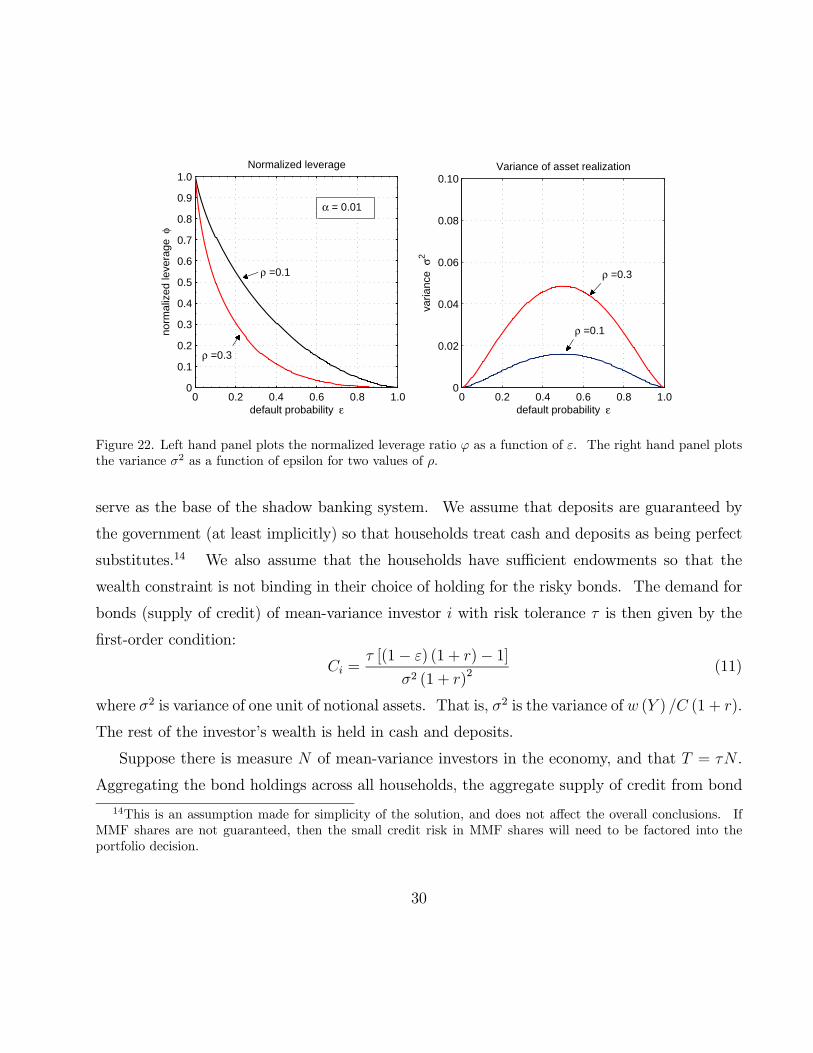
Figure 22. Left hand panel plots the normalized leverage ratio as a function of . The right hand panel plots
the variance 2 as a function of epsilon for two values of .
serve as the base of the shadow banking system. We assume that deposits are guaranteed by
the government (at least implicitly) so that households treat cash and deposits as being perfect
substitutes.14 We also assume that the households have sufficient endowments so that the
wealth constraint is not binding in their choice of holding for the risky bonds. The demand for
bonds (supply of credit) of mean-variance investor with risk tolerance is then given by the
first-order condition:
= [(1− ) (1 + )− 1]
2 (1 + )2
(11)
where 2 is variance of one unit of notional assets. That is, 2 is the variance of ( ) (1 + ).
The rest of the investor’s wealth is held in cash and deposits.
Suppose there is measure of mean-variance investors in the economy, and that = .
Aggregating the bond holdings across all households, the aggregate supply of credit from bond
14This is an assumption made for simplicity of the solution, and does not affect the overall conclusions. If
MMF shares are not guaranteed, then the small credit risk in MMF shares will need to be factored into the
portfolio decision.
30
investors is thus given by:
= [(1− ) (1 + )− 1]
2 (1 + )2
(12)
“” stands for the “household” sector. In the appendix, we show that the variance 2 is given
by
2 = Φ2¡Φ−1 () Φ−1 () ;
¢− 2 (13)
where Φ2 (· ·; ) is the cumulative bivariate standard normal with correlation .15 The right
hand panel of Figure 22 plots the variance 2 as a function of . The variance is maximized
when = 05, and is increasing in . The left hand panel of Figure 22 plots the normalized
leverage as a function of .
Since bank liabilities are fully guaranteed by the government they earn the risk-free rate.
Further, let the risk-free rate be zero, so that = 0. Since bank credit supply is increasing in
while bond investor credit supply is decreasing in 2, the effect of an increase in (assuming
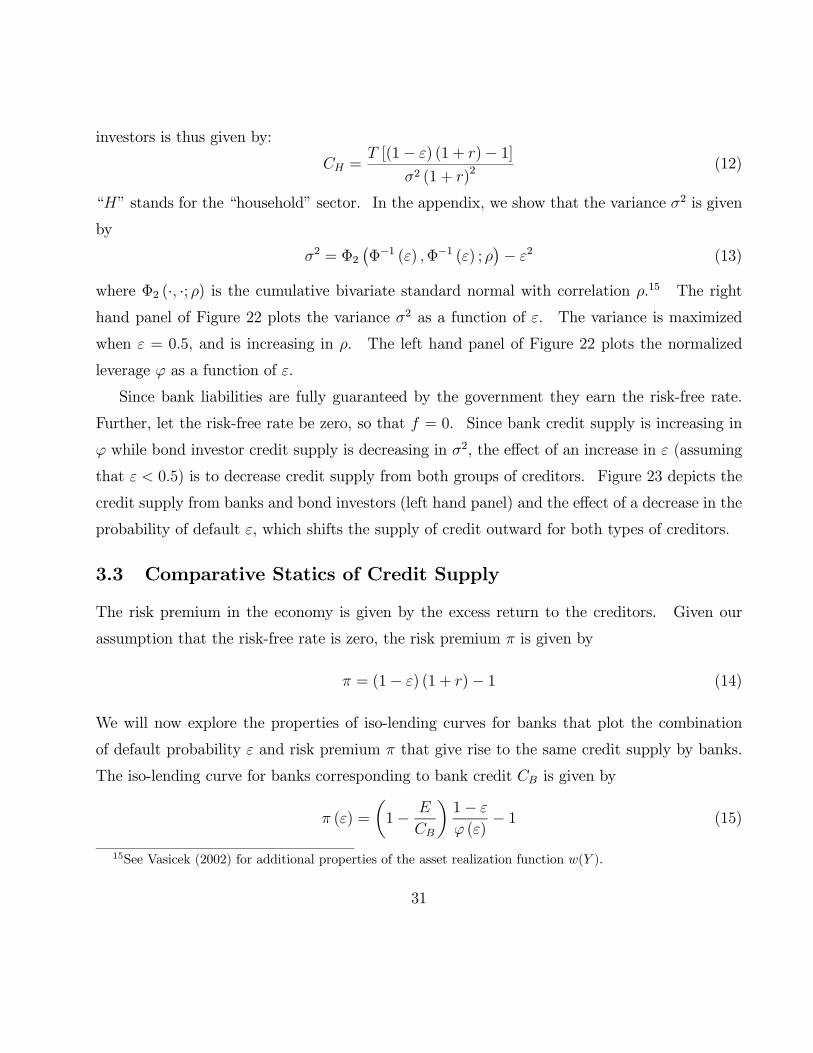
that 05) is to decrease credit supply from both groups of creditors. Figure 23 depicts the
credit supply from banks and bond investors (left hand panel) and the effect of a decrease in the
probability of default , which shifts the supply of credit outward for both types of creditors.
3.3 Comparative Statics of Credit Supply
The risk premium in the economy is given by the excess return to the creditors. Given our
assumption that the risk-free rate is zero, the risk premium is given by
= (1− ) (1 + )− 1 (14)
We will now explore the properties of iso-lending curves for banks that plot the combination
of default probability and risk premium that give rise to the same credit supply by banks.
The iso-lending curve for banks corresponding to bank credit is given by
() =
µ1−
¶1−
()− 1 (15)
15See Vasicek (2002) for additional properties of the asset realization function ( ).
31
0 100 200 3000.1
0.2
0.3
0.4
0.5
0.6
0.7
0.8
Bank and bond credit supply
Credit supply C
lend
ing
rate
r
0 100 200 3000.1
0.2
0.3
0.4
0.5
0.6
0.7
0.8
Credit supply increase due to fall in ε
Credit supply C
lend
ing
rate
r
bank creditsupply
total creditsupply
bond creditsupply
ε =0.1
ε =0.09
α = 0.01ρ = 0.3ε = 0.1E = 20T = 3
α = 0.01ρ = 0.3E = 20T = 3
Figure 23. This Figure depicts credit supply from banks and bond investors (left hand panel) and the effect of
a fall in from 0.1 to 0.09. The other parameters are as indicated in the box.
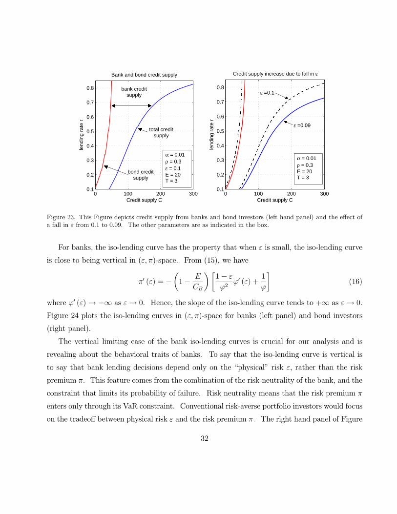
For banks, the iso-lending curve has the property that when is small, the iso-lending curve
is close to being vertical in ( )-space. From (15), we have
0 () = −µ1−
¶ ∙1−
20 () +
1
¸(16)
where 0 ()→−∞ as → 0. Hence, the slope of the iso-lending curve tends to +∞ as → 0.
Figure 24 plots the iso-lending curves in ( )-space for banks (left panel) and bond investors
(right panel).
The vertical limiting case of the bank iso-lending curves is crucial for our analysis and is
revealing about the behavioral traits of banks. To say that the iso-lending curve is vertical is
to say that bank lending decisions depend only on the “physical” risk , rather than the risk
premium . This feature comes from the combination of the risk-neutrality of the bank, and the
constraint that limits its probability of failure. Risk neutrality means that the risk premium
enters only through its VaR constraint. Conventional risk-averse portfolio investors would focus
on the tradeoff between physical risk and the risk premium . The right hand panel of Figure
32
0 0.1 0.2 0.3 0.40
0.2
0.4
0.6
0.8
1.0
Iso−lending curves for banks
default probability ε
risk
prem
ium
π
0 0.1 0.2 0.3 0.40
0.2
0.4
0.6
0.8
1.0
Iso−lending curves for bond investors
default probability ε
risk
prem
ium
π
α = 0.01ρ = 0.3E = 1
CB =10
CB =2
CH
= 2
CH
= 3
α = 0.01ρ = 0.3T = 2
CB =1.5
Figure 24. Iso-lending curves in ( )-space for banks (left panel) and bond investors (right panel). Parameter
values are as indicated in the boxes.
24 shows the iso-lending curves of the bond investors, to be derived shortly. Although we have
used mean-variance preferences for convenience for the bond investors, any conventional risk
averse preferences would imply a non-trivial tradeoff between physical risk and risk premium.
The fact that this tradeoff disappears for banks is key to understanding the Global Banking
Glut.
In the Mundell-Fleming model, capital flows are considered in a simple financial market
setting where investors are motivated by the relative interest rates across countries. The
implicit portfolio decisions did not contend with fluctuations in risk appetite of the investors
concerned. However, the introduction of the banking sector creates several unfamiliar features.
For instance, the leverage constraint of the banks gives rise to behavior where the banks act
as if their attitudes to risk change depending on the market outcome. During a boom, a
favorable shock increases risk-bearing capacity, and induces banks to lend more by borrowing
more. Thus, the favorable shock acts to change the banks’ “as if” preferences (see Shin (2010)
for more detailed discussion). The resulting demand and supply responses can be perverse,
33
giving rise to upward-sloping demand responses and downward-sloping supply responses.
Understanding the special nature of banking brings us closer to grasping the impact of
banking sector fluctuations for financial conditions, and the comparative statics results to be
reported below reveal key aspects. Our results do not rest on mean-variance preferences of the
bond investors. They depend only on the fact that bond investors have iso-lending curves that
have shallower slopes as compared to the banks. As long as banks and bond investors differ
in their behavioral characteristics, the relative weight of banks and bond investors in the credit
market will shift to changes in fundamentals. It is the shifting weight of the banking sector
that has important implications for economy-wide financial conditions.
The bond investors’ iso-lending curves in ( )-space follow from the supply of credit by
bond investors given by (12), from which we can derive the following quadratic equation in
2
(1− )2(1 + )
2 − (1 + ) + 1 = 0 (17)
The iso-lending curve for bond investors corresponding to bond credit supply of is given by
() =1−
q1− 42 (1− )
2
22 (1− )2
− 1 (18)
3.4 Comparative Statics of Risk Premium
Let us now close the model by positing an aggregate demand for credit. The demand for credit
is a decreasing function of the risk premium, and is denoted by (). The market clearing
condition is then
1− 1+1−| {z }
+ (1− )
2
2 (1 + )2| {z }
= () (19)
We can address our first substantive question. How does the risk premium vary to shifts
in the physical risks ? Provided that is small - so that it lies in the plausible range for the
probability of default - and provided that the risk premium is not too large, the risk premium
is an increasing function of .
34
Proposition 1 Suppose is small so that || (1− ) and the risk premium is small
so that 1. Then the market risk premium is strictly increasing in .
In other words, an increase in physical risk also raises the market risk premium. More
relevant for our narrative of the subprime crisis is the reverse effect. A decline in the physical
risk compresses the market risk premium , allowing lower quality projects to be funded.
To prove Proposition 1, note first that credit supply by bond investors is declining in ,
and that bank lending declines in if || (1− ). Meanwhile, we can also show
0 and - assuming 1 - we also have 0. Defining the excess supply of
credit function ( ) ≡ + − (), we have
= −
= −
+
+
− 0 ()
0 (20)
Since bank credit is declining in , the balance sheet identity implies that the funding used
by banks is also declining. We thus have the following important corollary to Proposition 1.
Corollary 2 Confining shocks to the economy to those on the default probability , aggregate
bank liabilities increase if and only if the market risk premium decreases.
Corollary 2 points to a possible rationale for tracking bank liability aggregates in the economy.
Tracking may be a useful window on the financial conditions in the economy, since it mirrors
the credit risk premium . The larger is , the more compressed is , and hence the lower are
lending standards in the economy, allowing lower quality projects to be funded. Our model
is not sufficiently developed to make welfare claims on whether the lower credit standards are
“excessively” low. The claim is merely a comparative statics claim that larger is associated
with lower .
Bank liabilities could be seen as a version of a monetary aggregate, and so Corollary 2
could be interpreted as a rationale for tracking monetary aggregates. However, the motivation
for monitoring in our context is very different from the traditional monetarist motivation
arising from the quantity theory of money and the focus on inflation. Indeed, in real world
35

implementation of monitoring bank liability aggregates, the focus could be on the most volatile
and procyclical components of bank liability aggregates - the “non-core” liabilities of the banking
sector. Shin and Shin (2010) discuss the rationale for monitoring non-core liabilities for financial
stability purposes, and Hahm, Shin and Shin (2011) show in a panel probit study of emerging
and developing economy financial crises that non-core liabilities figure strongly in explaining
financial crises.
Paradoxically, it is when the quantity of short-term, apparently “safe” liabilities of banks are
at their largest that the risk premiums ruling in the economy are at their lowest. However, the
paradox is only apparent once we realize that the short-term “safe” claims held by households
are funding sources for financial intermediaries who use the funding they receive to pass on
credit to ultimate borrowers. Since financial intermediaries are aggressive lenders when the risk
premium is low, their funding aggregates are large precisely when they are lending aggressively,
and when lending standards are being eroded. This interpretation of the role of apparently
“safe” short-term claims is at variance with accounts that emphasize an exogenous shift in
preferences to holding such safe claims, and explains to some extent why the money market
sector assets in Figure 17 see such large fluctuations over the financial cycle.
In our model, determined by the banks’ leverage decision. In practice, however, the
portfolio decision of depositors would also matter. Rather than the banks “sucking in” funding
from depositors, we could, alternatively, see the depositors “throwing themselves at” the banks in
their portfolio decision. Poszar (2011) takes the latter perspective and emphasizes the demand
for short-term cash-like claims by asset management firms who operate large “cash pools”.
Ascertaining the relative magnitudes of “demand pull” and “supply push” elements in de-
termining banking sector liability aggregates would entail careful empirical analysis, possibly
through methods such as vector autoregressions with sign restrictions that can identify demand
and supply driven responses. Even here, however, some caution is required. In the shadow
banking system, with many-layered intermediaries, the funding to one intermediary is supplied
by another intermediary. For instance, when broker dealers borrow through a securities repo,
the creditor may be another intermediary. As such, any empirical determination of the relative
36
strength of demand push and supply pull forces should ideally focus on the final stage of the
intermediation chain to the extent possible.
3.5 Relative Size of Banking Sector
We now address another stylized fact concerning the size of the banking sector and the vulner-
ability to a reversal. Specifically, when the default probability declines, what happens to the
size of the banking sector - both in absolute terms, and in relative terms compared to the bond
investor sector? Proposition 3 addresses these questions. Provided that credit demand ()
is not too elastic, a decline in is followed by an increase in the size of the banking sector, both
in absolute terms and as a proportion to the total credit provided in the economy.
Proposition 3 Suppose that is small enough so that the iso-lending curve of banks is steeper
than the iso-lending curve of bond investors. Then, there is 0 such that, provided | 0 ()| ≤ , a decline in is associated with an increase in banking sector assets, both in absolute terms
and as a proportion of the total credit received by borrowers.
Proposition 3 can be proved using a graphical argument using the iso-lending curves for
banks and bond investors. Figure 25 illustrates an initial equilibrium given by the crossing
point for the iso-lending curves for banks and bond investors. In this illustration, total credit
supply is 20, with 10 coming from banks and 10 coming from bond investors. The four regions
indicated in Figure 25 correspond to the four combinations of credit supply changes by banks
and bond investors. Region A is when both banks and bond investors increase credit supply,
while Region C is where both reduce credit supply.
Now, consider a fall in that puts us to the left side of the banks’ iso-lending curve, implying
an increase in bank credit. In addition, the market risk premium falls, as a consequence of
Proposition 1.
Consider first the benchmark case where the credit demand curve is vertical, so that 0 () =
0. Then, we have the combination of an increase in bank credit supply while total credit supply
is unchanged, implying that bond credit supply must fall for the market to clear. Thus, the
37
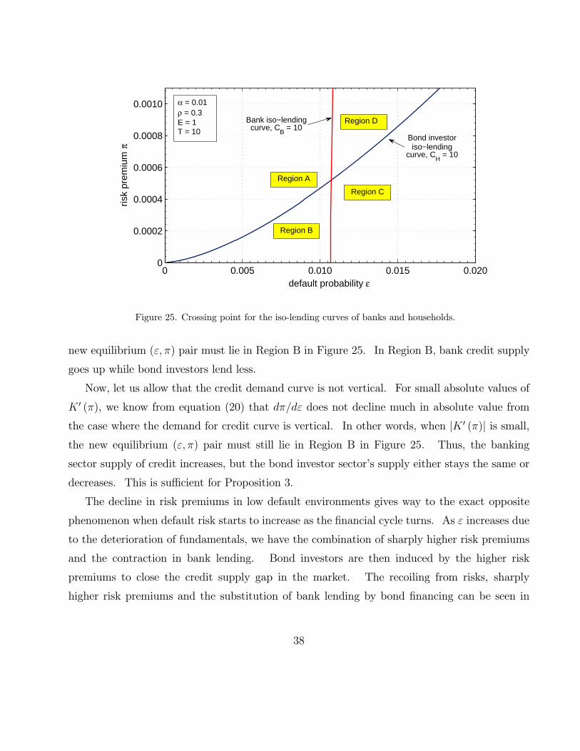
0 0.005 0.010 0.015 0.0200
0.0002
0.0004
0.0006
0.0008
0.0010
m
risk
prem
ium
πRegion D
α = 0.01ρ = 0.3E = 1T = 10
Region C
Region A
Region B
Bond investoriso−lending
curve, CH
= 10
Bank iso−lendingcurve, C
B = 10
default probability ε
Figure 25. Crossing point for the iso-lending curves of banks and households.
new equilibrium ( ) pair must lie in Region B in Figure 25. In Region B, bank credit supply
goes up while bond investors lend less.
Now, let us allow that the credit demand curve is not vertical. For small absolute values of
0 (), we know from equation (20) that does not decline much in absolute value from
the case where the demand for credit curve is vertical. In other words, when | 0 ()| is small,the new equilibrium ( ) pair must still lie in Region B in Figure 25. Thus, the banking
sector supply of credit increases, but the bond investor sector’s supply either stays the same or
decreases. This is sufficient for Proposition 3.
The decline in risk premiums in low default environments gives way to the exact opposite
phenomenon when default risk starts to increase as the financial cycle turns. As increases due
to the deterioration of fundamentals, we have the combination of sharply higher risk premiums
and the contraction in bank lending. Bond investors are then induced by the higher risk
premiums to close the credit supply gap in the market. The recoiling from risks, sharply
higher risk premiums and the substitution of bank lending by bond financing can be seen in
38
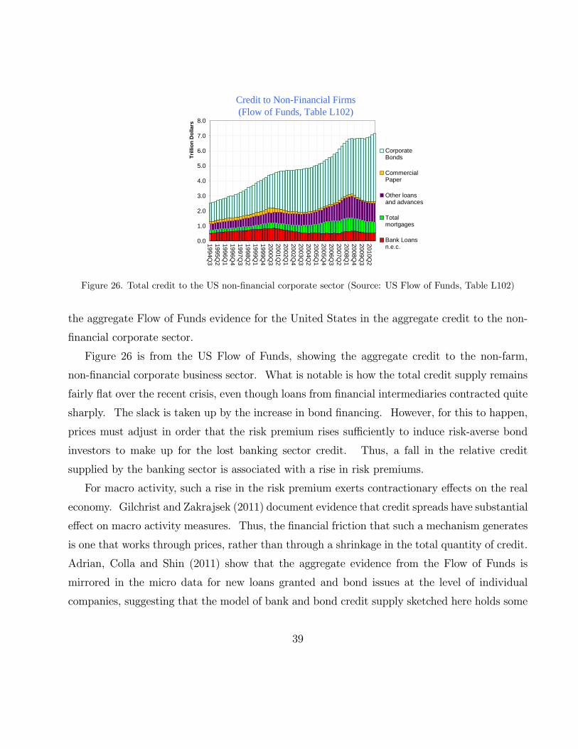
Credit to Non-Financial Firms (Flow of Funds, Table L102)
0.0
1.0
2.0
3.0
4.0
5.0
6.0
7.0
8.0
1994Q3
1995Q2
1996Q1
1996Q4
1997Q3
1998Q2
1999Q1
1999Q4
2000Q3
2001Q2
2002Q1
2002Q4
2003Q3
2004Q2
2005Q1
2005Q4
2006Q3
2007Q2
2008Q1
2008Q4
2009Q3
2010Q2
Tri
llio
n D
olla
rs
CorporateBonds
CommercialPaper
Other loansand advances
Totalmortgages
Bank Loansn.e.c.
Figure 26. Total credit to the US non-financial corporate sector (Source: US Flow of Funds, Table L102)
the aggregate Flow of Funds evidence for the United States in the aggregate credit to the non-
financial corporate sector.
Figure 26 is from the US Flow of Funds, showing the aggregate credit to the non-farm,
non-financial corporate business sector. What is notable is how the total credit supply remains
fairly flat over the recent crisis, even though loans from financial intermediaries contracted quite
sharply. The slack is taken up by the increase in bond financing. However, for this to happen,
prices must adjust in order that the risk premium rises sufficiently to induce risk-averse bond
investors to make up for the lost banking sector credit. Thus, a fall in the relative credit
supplied by the banking sector is associated with a rise in risk premiums.
For macro activity, such a rise in the risk premium exerts contractionary effects on the real
economy. Gilchrist and Zakrajsek (2011) document evidence that credit spreads have substantial
effect on macro activity measures. Thus, the financial friction that such a mechanism generates
is one that works through prices, rather than through a shrinkage in the total quantity of credit.
Adrian, Colla and Shin (2011) show that the aggregate evidence from the Flow of Funds is
mirrored in the micro data for new loans granted and bond issues at the level of individual
companies, suggesting that the model of bank and bond credit supply sketched here holds some
39
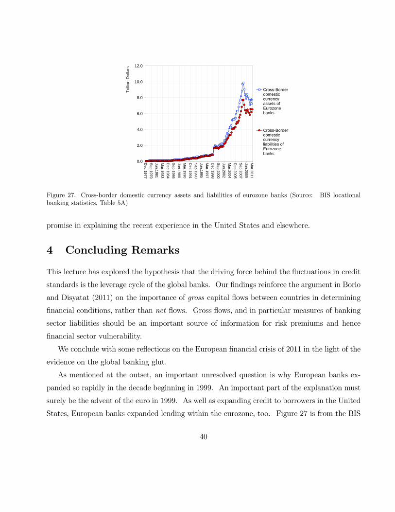
0.0
2.0
4.0
6.0
8.0
10.0
12.0
Dec.1977
Sep.1979
Jun.1981
Mar.1983
Dec.1984
Sep.1986
Jun.1988
Mar.1990
Dec.1991
Sep.1993
Jun.1995
Mar.1997
Dec.1998
Sep.2000
Jun.2002
Mar.2004
Dec.2005
Sep.2007
Jun.2009
Mar.2011
Tril
lion
Dol
lars
Cross-Borderdomesticcurrencyassets ofEurozonebanks
Cross-Borderdomesticcurrencyliabilities ofEurozonebanks
Figure 27. Cross-border domestic currency assets and liabilities of eurozone banks (Source: BIS locational
banking statistics, Table 5A)
promise in explaining the recent experience in the United States and elsewhere.
4 Concluding Remarks
This lecture has explored the hypothesis that the driving force behind the fluctuations in credit
standards is the leverage cycle of the global banks. Our findings reinforce the argument in Borio
and Disyatat (2011) on the importance of gross capital flows between countries in determining
financial conditions, rather than net flows. Gross flows, and in particular measures of banking
sector liabilities should be an important source of information for risk premiums and hence
financial sector vulnerability.
We conclude with some reflections on the European financial crisis of 2011 in the light of the
evidence on the global banking glut.
As mentioned at the outset, an important unresolved question is why European banks ex-
panded so rapidly in the decade beginning in 1999. An important part of the explanation must
surely be the advent of the euro in 1999. As well as expanding credit to borrowers in the United
States, European banks expanded lending within the eurozone, too. Figure 27 is from the BIS
40
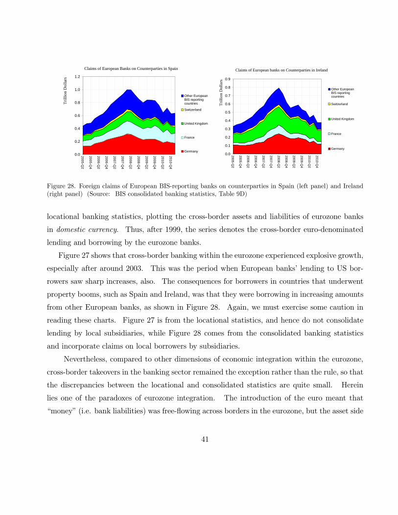
Claims of European Banks on Counterparties in Spain
0.0
0.2
0.4
0.6
0.8
1.0
1.2
20
05
-Q2
20
05
-Q4
20
06
-Q2
20
06
-Q4
20
07
-Q2
20
07
-Q4
20
08
-Q2
20
08
-Q4
20
09
-Q2
20
09
-Q4
20
10
-Q2
20
10
-Q4
Tri
llio
n D
olla
rs
Other EuropeanBIS reportingcountries
Switzerland
United Kingdom
France
Germany
Claims of European banks on Counterparties in Ireland
0.0
0.1
0.2
0.3
0.4
0.5
0.6
0.7
0.8
0.9
2005-Q2
2005-Q4
2006-Q2
2006-Q4
2007-Q2
2007-Q4
2008-Q2
2008-Q4
2009-Q2
2009-Q4
2010-Q2
2010-Q4
Tri
llio
n D
olla
rs
Other EuropeanBIS reportingcountries
Switzerland
United Kingdom
France
Germany
Figure 28. Foreign claims of European BIS-reporting banks on counterparties in Spain (left panel) and Ireland
(right panel) (Source: BIS consolidated banking statistics, Table 9D)
locational banking statistics, plotting the cross-border assets and liabilities of eurozone banks
in domestic currency. Thus, after 1999, the series denotes the cross-border euro-denominated
lending and borrowing by the eurozone banks.
Figure 27 shows that cross-border banking within the eurozone experienced explosive growth,
especially after around 2003. This was the period when European banks’ lending to US bor-
rowers saw sharp increases, also. The consequences for borrowers in countries that underwent
property booms, such as Spain and Ireland, was that they were borrowing in increasing amounts
from other European banks, as shown in Figure 28. Again, we must exercise some caution in
reading these charts. Figure 27 is from the locational statistics, and hence do not consolidate
lending by local subsidiaries, while Figure 28 comes from the consolidated banking statistics
and incorporate claims on local borrowers by subsidiaries.
Nevertheless, compared to other dimensions of economic integration within the eurozone,
cross-border takeovers in the banking sector remained the exception rather than the rule, so that
the discrepancies between the locational and consolidated statistics are quite small. Herein
lies one of the paradoxes of eurozone integration. The introduction of the euro meant that
“money” (i.e. bank liabilities) was free-flowing across borders in the eurozone, but the asset side
41
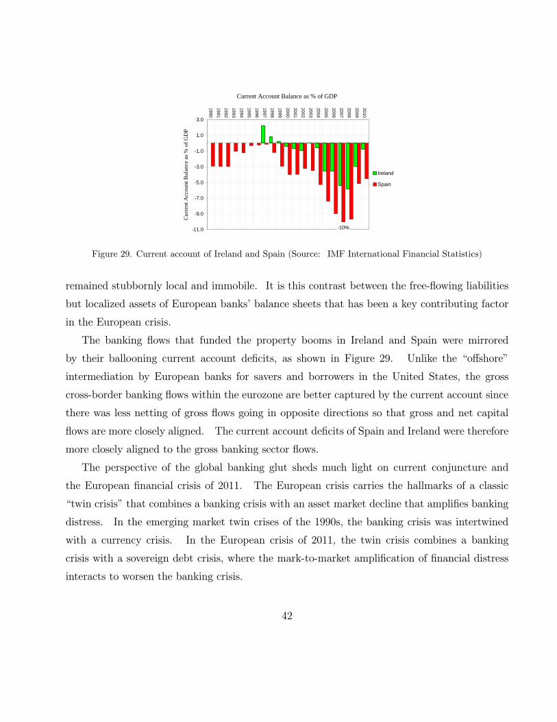
Current Account Balance as % of GDP
-10%-11.0
-9.0
-7.0
-5.0
-3.0
-1.0
1.0
3.0
19
90
19
91
19
92
19
93
19
94
19
95
19
96
19
97
19
98
19
99
20
00
20
01
20
02
20
03
20
04
20
05
20
06
20
07
20
08
20
09
20
10
Cur
rent
Acc
ount
Bal
ance
as
% o
f G
DP
Ireland
Spain
Figure 29. Current account of Ireland and Spain (Source: IMF International Financial Statistics)
remained stubbornly local and immobile. It is this contrast between the free-flowing liabilities
but localized assets of European banks’ balance sheets that has been a key contributing factor
in the European crisis.
The banking flows that funded the property booms in Ireland and Spain were mirrored
by their ballooning current account deficits, as shown in Figure 29. Unlike the “offshore”
intermediation by European banks for savers and borrowers in the United States, the gross
cross-border banking flows within the eurozone are better captured by the current account since
there was less netting of gross flows going in opposite directions so that gross and net capital
flows are more closely aligned. The current account deficits of Spain and Ireland were therefore
more closely aligned to the gross banking sector flows.
The perspective of the global banking glut sheds much light on current conjuncture and
the European financial crisis of 2011. The European crisis carries the hallmarks of a classic
“twin crisis” that combines a banking crisis with an asset market decline that amplifies banking
distress. In the emerging market twin crises of the 1990s, the banking crisis was intertwined
with a currency crisis. In the European crisis of 2011, the twin crisis combines a banking
crisis with a sovereign debt crisis, where the mark-to-market amplification of financial distress
interacts to worsen the banking crisis.
42
The global flow of funds perspective suggests that the European crisis of 2011 and the
associated deleveraging of the European global banks will have far reaching implications not
only for the eurozone, but also for credit supply conditions in the United States and capital
flows to the emerging economies.
In this lecture, I have argued that global liquidity is a banking sector phenomenon, and
that the financial stability implications of global liquidity are intimately tied to the leverag-
ing/deleveraging cycle of the global banks. Much work remains to be done in exploring the
implications for macroprudential policy.
43
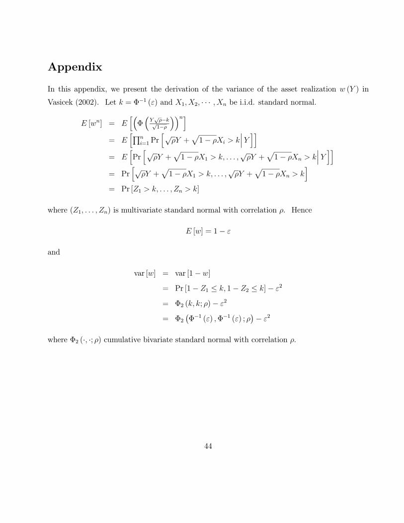
Appendix
In this appendix, we present the derivation of the variance of the asset realization ( ) in
Vasicek (2002). Let = Φ−1 () and 1 2 · · · be i.i.d. standard normal.
[] = h³
Φ³√−√1−
´´i=
hQ
=1 Prh√
+p1−
¯ii
= hPrh√
+p1− 1
√ +
p1−
¯ii
= Prh√
+p1− 1
√ +
p1−
i= Pr [1 ]
where (1 ) is multivariate standard normal with correlation . Hence
[] = 1−
and
var [] = var [1− ]
= Pr [1− 1 ≤ 1− 2 ≤ ]− 2
= Φ2 ( ; )− 2
= Φ2¡Φ−1 () Φ−1 () ;
¢− 2
where Φ2 (· ·; ) cumulative bivariate standard normal with correlation .
44
References
Acharya, Viral and Philipp Schanbl (2009) “Do Global Banks Spread Global Imbalances? The
Case of Asset-Backed Commercial Paper during the Financial Crisis of 2007-09” IMF Economic
Review, 58, 2010, 37-73.
Adrian, Tobias, Paolo Colla and Hyun Song Shin (2011) “Which Financial Frictions? Parsing
the Evidence from the Financial Crisis of 2007-9” working paper.
Adrian, Tobias and Hyun Song Shin (2008) “Procyclical Leverage and Value-at-Risk” Federal
Reserve Bank of New York Staff Report 338,
http://www.newyorkfed.org/research/staff reports/sr338.html
Adrian, Tobias and Hyun Song Shin (2010) “Liquidity and Leverage,” Journal of Financial
Intermediation, 19, 418-437
Baba, Naohiko, Robert N. McCauley and Srichander Ramaswamy (2009) “US Dollar Money
Market Funds and Non-US Banks” BIS Quarterly Review, March 2009, 65-81.
Bank for International Settlements (2009) “Guide to the international financial statistics”
http://www.bis.org/statistics/intfinstatsguide.pdf
Bank for International Settlements (2010) “Funding patterns and liquidity management of in-
ternationally active banks” CGFS Papers 39, Committee on the Global Financial System, May
Basel Committee on Banking Supervision (2005) “International Convergence of Capital Mea-
surement and Capital Standards: A Revised Framework”, Bank for International Settlements,
November 2005 http://www.bis.org/publ/bcbs118.pdf
Bernanke, Ben S. (2005) “The Global Saving Glut and the U.S. Current Account Deficit”,
Remarks at the Sandridge Lecture, Virginia Association of Economists, Richmond, Virginia,
March 10, 2005, http://www.federalreserve.gov/boarddocs/speeches/2005/200503102/
Bernanke, Ben S., Carol Bertaut, Laurie Pounder DeMarco, and Steven Kamin (2011) “In-
ternational Capital Flows and the Returns to Safe Assets in the United States, 2003-2007”,
International Finance Discussion Papers Number 1014, Board of Governors of the Federal Re-
serve System, http://www.federalreserve.gov/pubs/ifdp/2011/1014/ifdp1014.htm
Bertaut, Carol, Laurie Pounder DeMarco, Steven Kamin and Ralph Tryon (2011) “ABS Inflows
to the United States and the Global Financial Crisis” Board of Governors of the Federal Reserve
System International Finance Discussion Paper 1028, August 2011
http://www.federalreserve.gov/pubs/ifdp/2011/1028/ifdp1028.pdf
45
Borio, Claudio and Piti Disyatat (2011) “Global imbalances and the financial crisis: Link or no
link?” BIS Working Papers No 346 http://www.bis.org/publ/work346.pdf
Borio, Claudio and Haibin Zhu (2008) “Capital regulation, risk-taking and monetary policy: a
missing link in the transmission mechanism?” BIS Working Papers, no 268
Bruno, Valentina and Hyun Song Shin (2011) “Capital Flows, Cross-Border Banking and Global
Liquidity” working paper
Caballero, Ricardo J., Emmanuel Farhi, and Pierre-Olivier Gourinchas (2008) ”An Equilibrium
Model of ”Global Imbalances” and Low Interest Rates.” American Economic Review, 98(1):
358—93.
Cetorelli, Nicola and Linda S. Goldberg (2009) “Banking Globalization and Monetary Trans-
mission” Forthcoming in Journal of Finance.
Cetorelli, Nicola and Linda S. Goldberg (2010) “Global Banks and International Shock Trans-
mission: Evidence from the Crisis”, Federal Reserve Bank of New York Staff Report #446.
Danielsson, Jon, Paul Embrechts, Charles Goodhart, Felix Muennich, Con Keating, Olivier Re-
nault and Hyun Song Shin (2001) “An Academic Response to Basel II” Financial Markets Group
Special Paper 130, London School of Economics http://hyunsongshin.org/www/basel2.pdf
European Central Bank (2011) Financial Stability Review, June 2011, ECB Frankfurt
http://www.ecb.eu/pub/fsr/html/index.en.html
Fleming, J. Marcus (1962). “Domestic financial policies under fixed and floating exchange
rates”. IMF Staff Papers 9: 369—379.
Gilchrist, Simon, and Egon Zakrajsek (2011) “Credit Spreads and Business Cycle Fluctuations”,
forthcoming in the American Economic Review.
Gourinchas, Pierre-Olivier and Helene Rey (2007) “International Financial Adjustment” Journal
of Political Economy, 115(4), 665-703
Gourinchas, Pierre-Olivier, Nicolas Govillot and Helene Rey (2010) “Exorbitant Privilege and
Exorbitant Duty” working paper
Hahm, Joon-Ho, Hyun Song Shin and Kwanho Shin (2011) “Non-Core Bank Liabilities and
Financial Vulnerability” working paper.
46
Kindleberger, Charles (1965) “Balance of Payments Deficits and the International Market for
Liquidity” Princeton Essays in International Finance No. 46, May 1965,
http://www.princeton.edu/˜ies/old series-win.htm
Lane, Philip and Gian Maria Milesi-Ferretti (2007). ”The External Wealth of Nations Mark
II: Revised and Extended Estimates of Foreign Assets and Liabilities, 1970—2004” Journal of
International Economics, 73, 223-250.
McGuire, Patrick and Goetz von Peter (2009) “The US Dollar Shortage in Global Banking”
BIS Quarterly Review, March 2009, Bank for International Settlements.
Milesi-Ferretti, Gian Maria (2009) “Notes on the financial crisis and global financial architecture”
in Causes of the Crisis: Key Lessons, proceedings of the G20 workshop on the Global Economy.
Mumbai, May 2009, http://www.g20.org/Documents/g20 workshop causes of the crisis.pdf
Mundell, Robert A. (1963). ”Capital mobility and stabilization policy under fixed and flexible
exchange rates”. Canadian Journal of Economic and Political Science 29 (4): 475—485.
Pozsar, Zoltan (2011) “Institutional Cash Pools and the Triffin Dilemma of the U.S. Banking
System” IMF Working Paper, WP/11/190, August 2011
Shin, Hyun Song (2010) Risk and Liquidity, 2008 Clarendon Lectures in Finance, Oxford Uni-
versity Press, Oxford.
Shin, Hyun Song and Kwanho Shin (2010) “Procyclicality and Monetary Aggregates”, NBER
working paper w16836, http://www.nber.org/papers/w16836.
Vasiceck, Oldrich (2002) “The Distribution of Loan Portfolio Value” Risk, December 2002,
http://www.moodyskmv.com/conf04/pdf/papers/dist loan port val.pdf
47