giuliog/opencbv.pdf · open call-by-value beniamino accattoli1 and giulio guerrieri2 1 inria, umr...

Open Call-by-Value

Beniamino Accattoli1 and Giulio Guerrieri2

1 INRIA, UMR 7161, LIX, Ecole Polytechnique, [email protected],2 Aix Marseille Universite, I2M UMR 7373, [email protected]

Abstract. The elegant theory of the call-by-value lambda-calculus relieson weak evaluation and closed terms, that are natural hypotheses in thestudy of programming languages. To model proof assistants, however,strong evaluation and open terms are required, and it is well known thatthe operational semantics of call-by-value becomes problematic in thiscase. Here we study the intermediate setting—that we call Open Call-by-Value—of weak evaluation with open terms, on top of which Gregoire andLeroy designed the abstract machine of Coq. Various calculi for OpenCall-by-Value already exist, each one with its pros and cons. This paperpresents a detailed comparative study of the operational semantics offour of them, coming from different areas such as the study of abstractmachines, denotational semantics, linear logic proof nets, and sequentcalculus. We show that these calculi are all equivalent from a terminationpoint of view, justifying the slogan Open Call-by-Value.

1 Introduction

Plotkin’s call-by-value λ-calculus [27] is at the heart of programming languagessuch as Ocaml and proof assistants such as Coq. In the study of programminglanguages, call-by-value (CBV) evaluation is usually weak, i.e. it does not reduceunder abstractions, and terms are assumed to be closed. These constraints giverise to a beautiful theory—let us call it Closed CBV —having the followingharmony property, that relates rewriting and normal forms:

Closed normal forms are values (and values are normal forms)

where values are variables and abstractions. Harmony expresses a form of internalcompleteness with respect to unconstrained β-reduction: the restriction to CBVβ-reduction (referred to as βv-reduction, according to which a β-redex can befired only when the argument is a value) has an impact on the order in whichredexes are evaluated, but evaluation never gets stuck, as every β-redex willeventually become a βv-redex and be fired, unless evaluation diverges.

It often happens, however, that one needs to go beyond the perfect setting ofClosed CBV, by considering Strong CBV, where reduction under abstractions isallowed and terms may be open, or the intermediate setting of Open CBV, whereevaluation is weak but terms are not necessarily closed. The need arises, mostnotably, when trying to describe the implementation model of Coq [13], but alsofrom other motivations, as denotational semantics [26,29,3,8], monad and CPStranslations and the associated equational theories [22,30,31,12,17], bisimulations[19], partial evaluation [18], linear logic proof nets [2], or cost models [1].

mailto:[email protected]

mailto:[email protected]

2 B. Accattoli, G. Guerrieri

Naıve Open CBV. In call-by-name (CBN) turning to open terms or strongevaluation is harmless because CBN does not impose any special form to thearguments of β-redexes. On the contrary, turning to Open or Strong CBV isdelicate. If one simply considers Plotkin’s weak βv-reduction on open terms—letus call it Naıve Open CBV —then harmony does no longer hold, as there areopen β-normal forms that are not values, e.g. xx, x(λy.y), x(yz) or xyz. As aconsequence, there are stuck β-redexes such as (λy.t)(xx), i.e. β-redexes thatwill never be fired because their argument is normal, but it is not a value, norwill it ever become one. Such stuck β-redexes are a disease typical of (Naıve)Open CBV, but they spread to Strong CBV as well (also in the closed case),because evaluating under abstraction forces to deal with locally open terms: e.g.the variable x is locally open with respect to (λy.t)(xx) in s = λx.((λy.t)(xx)).

The real issue with stuck β-redexes is that they prevent the creation of otherredexes, and provide premature βv-normal forms. The issue is serious, as it canaffect termination, and thus impact on notions of observational equivalence. Letδ := λx.(xx). The problem is exemplified by the terms t and u in Eq. (1) below.

t := ((λy.δ)(zz))δ u := δ((λy.δ)(zz)) (1)

In Naıve Open CBV, t and u are premature βv-normal forms because they bothhave a stuck β-redex forbidding evaluation to keep going, while one would expectthem to behave like the divergent term Ω := δδ (see [26,29,3,2,8,15] and pp. 7-12).

Open CBV. In his seminal work, Plotkin already pointed out an asymmetrybetween CBN and CBV: his CPS translation is sound and complete for CBN,but only sound for CBV. This fact led to a number of studies about monad, CPS,and logical translations [22,30,31,21,12,17] that introduced many proposals ofimproved calculi for CBV. Starting with the seminal work of Paolini and RonchiDella Rocca [26,24,29], the dissonance between open terms and CBV has beenrepeatedly pointed out and studied per se via various calculi [13,3,2,8,15,14,1]. Afurther point of view on CBV comes from the computational interpretation ofsequent calculus due to Curien and Herbelin [9]. An important point is that thefocus of most of these works is on Strong CBV.

These solutions inevitably extend βv-reduction with some other rule(s) orconstructor (as let-expressions) to deal with stuck β-redexes, or even go as far aschanging the applicative structure of λ-terms, as in the sequent calculus approach.They arise from different perspectives and each one has its pros and cons. Bydesign, these calculi (when looked at in the context of Open CBV) are neverobservationally equivalent to Naıve Open CBV, as they all manage to (re)movestuck β-redexes and may diverge when Naıve Open CBV is instead stuck. Eachone of these calculi, however, has its own notion of evaluation and normal form,and their mutual relationships are not evident.

The aim of this paper is to draw the attention of the community on OpenCBV. We believe that it is somewhat deceiving that the mainstream operationaltheory of CBV, however elegant, has to rely on closed terms, because it restrictsthe modularity of the framework, and raises the suspicion that the true essenceof CBV has yet to be found. There is a real gap, indeed, between Closed and

Open Call-by-Value 3

Strong CBV, as Strong CBV cannot be seen as an iteration of Closed CBVunder abstractions because such an iteration has to deal with open terms. Toimprove the implementation of Coq [13], Gregoire and Leroy see Strong CBV asthe iteration of the intermediate case of Open CBV, but they do not explore itstheory. Here we exalt their point of view, providing a thorough operational studyof Open CBV. We insist on Open CBV rather than Strong CBV because:

1. Stuck β-redexes and premature βv-normal forms are already in Open CBV;

2. Open CBV has a simpler rewriting theory than Strong CBV;

3. Our previous studies of Strong CBV in [3] and [8] naturally organized them-selves as properties of Open CBV that were lifted to Strong CBV by a simpleiteration under abstractions.

Our contributions are along two axes:

1. Termination Equivalence of the Proposals : we show that the proposed general-izations of Naıve Open CBV are equivalent, in the sense that they have exactlythe same sets of normalizing and diverging λ-terms. Therefore, there is justone notion of Open CBV, independently of its specific syntactic incarnation.

2. Quantitative Analyses and Cost Models: the termination results are comple-mented with quantitative analyses establishing precise relationships betweenthe number of steps needed to evaluate a given term in the various calculi. Inparticular, we relate the cost models of the various proposals.

Equivalence of the Proposals. We focus on four proposals for Open CBV, as othersolutions, e.g. Moggi’s [22] or Herbelin and Zimmerman’s [17], are already knownto be equivalent to these ones (see the end of Sect. 2):

1. The Fireball Calculus λfire, that extends values to fireballs by adding so-calledinert terms in order to restore harmony—it was introduced without a nameby Paolini and Ronchi Della Rocca [26,29], then rediscovered independentlyfirst by Leroy and Gregoire [13] to improve the implementation of Coq, andthen by Accattoli and Sacerdoti Coen [1] to study cost models;

2. The Value Substitution Calculus λvsub, coming from the linear logic interpre-tation of CBV and using explicit substitutions and contextual rewriting rulesto circumvent stuck β-redexes—it was introduced by Accattoli and Paolini [3]and it is a graph-free presentation of proof nets for the CBV λ-calculus [2];

3. The Shuffling Calculus λsh, that has rules to shuffle constructors, similar toRegnier’s σ-rules for CBN [28], as an alternative to explicit substitutions—itwas introduced by Carraro and Guerrieri [8] (and further analyzed in [15,14])to study the adequacy of Open/Strong CBV with respect to denotationalsemantics related to linear logic.

4. The Value Sequent Calculus λvseq, i.e. the intuitionistic fragment of the λµcalculus of Curien and Herbelin [9], that is a CBV calculus for classical logicproviding a computational interpretation of sequent calculus rather thannatural deduction (in turn a fragment of the λµµ-calculus [9], further studiedin e.g. [5,10]).

Quantitative Analyses and Cost Models. The number of βv-steps is the canonicaltime cost model of Closed CBV, as first proved by Blelloch and Greiner [7,32,11].


This result is generalized in [1]: the number of steps in λfire is a reasonablecost model for Open CBV. Here we show that the number of β-steps in λvsuband λvseq are linearly related to the steps in λfire, thus providing reasonablecost models for these incarnations of Open CBV. As a consequence, complexityanalyses can now be smoothly transferred between λfire, λvsub, and λvseq. Saiddifferently, our results guarantee that the number of steps is a robust cost modelfor Open CBV, in the sense that it does not depend on the chosen incarnation ofOpen CBV. For λsh we obtain a similar but strictly weaker result, due to somestructural difficulties suggesting that λsh is less apt to complexity analyses.

On the Value of The Paper. While the equivalences showed here are new, theymight not be terribly surprising. Nonetheless, we think they are interesting, forthe following reasons:

1. Quantitative Relationships: λ-calculi are usually related only qualitatively,while our relationships are quantitative and thus stronger: not only we showsimulations, but we also relate the number of steps.

2. Uniform View : we provide a new uniform view on a known problem, that willhopefully avoid further proliferations of CBV calculi for open/strong settings.

3. Expected but Non-Trivial : while the equivalences are more or less expected,establishing them is informative, because it forces to reformulate and connectconcepts among the different settings, and often tricky.

4. Simple Rewriting Theory : the relationships between the systems are developedusing basic rewriting concepts. The technical development is simple, accordingto the best tradition of the CBV λ-calculus, and yet it provides a sharp anddetailed decomposition of Open CBV evaluation.

5. Connecting Different Worlds: while λfire is related to Coq and implemen-tations, λvsub and λsh have a linear logic background, and λvseq is rooted insequent calculus. With respect to linear logic, λvsub has been used for syn-tactical studies while λsh for semantical ones. Our results therefore establishbridges between these different (sub)communities.

Finally, an essential contribution of this work is the recognition of Open CBVas a simple and yet rich framework in between Closed and Strong CBV.

Road map. Sect. 2 provides an overview of the different presentations of OpenCBV. Sect. 3 proves the termination equivalences for λvsub, λfire and λsh, enrichedwith quantitative information. Sect. 4 proves, with quantitative information, thetermination equivalence for λvsub and λvseq, via an intermediate calculus λvsubk .Appendix A (p. 19) collects the definitions and notations of the rewriting notionsat work in the paper. Omitted proofs are in Appendix B (p. 20). In case ofacceptance, this long version with Appendices will be made available on Arxiv.

2 Incarnations of Open Call-by-Value

Here we recall Naıve Open CBV λPlot and introduce the four forms of Open CBVthat will be compared (λfire, λvsub, λsh, and λvseq) together with a semanticnotion (potential valuability) reducing Open CBV to Closed CBV. In this paper


Terms t, u, s, r::=v | tuValues v, v′::=x | λx.t

Evaluation Contexts E::=〈·〉 | tE | Et

Rule at Top Level Contextual closure(λx.t)λy.u 7→βλ txλy.u E〈t〉 →βλ E〈u〉 if t 7→βλ u

(λx.t)y 7→βy txy E〈t〉 →βy E〈u〉 if t 7→βy u

Reduction →βv :=→βλ ∪ →βy

Fig. 1. Naıve Open CBV λPlot

terms are always possibly open. Moreover, we focus on Open CBV and avoid onpurpose to study Strong CBV (we hint at how to define it, though).

Naıve Open CBV: Plotkin’s calculus λPlot [27] Naıve Open CBV is Plotkin’s weakCBV λ-calculus λPlot on possibly open terms, defined in Fig. 1. Our presentationof the rewriting is unorthodox because we split βv-reduction into two rules,according to the kind of value (abstraction or variable). The set of terms isdenoted by Λ. Terms (in Λ) are always identified up to α-equivalence and theset of the free variables of a term t is denoted by fv(t). We use txu for theterm obtained by the capture-avoiding substitution of u for each free occurrenceof x in t. Evaluation →βv is weak and non-deterministic, since in the case of anapplication there is no fixed order in the evaluation of the left and right subterms.As it is well-known, non-determinism is only apparent: the system is stronglyconfluent (see Appendix A for a glossary and notations of rewriting theory).

Proposition 1. →βy , →βλ and →βv are strongly confluent. Proof p. 20

Strong confluence is a remarkable property, much stronger than plain con-fluence. It implies that, given a term, all derivations to its normal form (if any)have the same length, and that normalization and strong normalization coincide,i.e. if there is a normalizing derivation then there are no diverging derivations.Strong confluence will also hold for λfire, λvsub and λvseq, not for λsh.

Let us come back to the splitting of→βv . In Closed CBV it is well-known that→βy is superfluous, at least as long as small-step evaluation is considered, see [4].For Open CBV, →βy is instead necessary, but—as we explained in Sect. 1—it isnot enough, which is why we shall consider extensions of λPlot. The main problemof Naıve Open CBV is that there are stuck β-redexes that break the harmony ofthe system. There are three kinds of solution: those restoring a form of harmony(λfire), to be thought as more semantical approaches; those removing stuckβ-redexes (λvsub and λsh), that are more syntactical in nature; those changingthe applicative structure of λ-terms (λvseq), inspired by sequent calculus.

Open Call-by-Value 1: The Fireball Calculus λfire. The Fireball Calculus λfire,defined in Fig. 2, was introduced without a name by Paolini and Ronchi DellaRocca in [26] and [29, Def. 3.1.4, p. 36] where its basic properties are also proved.We give here a presentation inspired by Accattoli and Sacerdoti Coen’s [1],


Terms and Values As in Plotkin’s Open CBV (Fig. 1)Fireballs f, f ′, f ′′ ::= λx.t | i

Inert Terms i, i′, i′′ ::= xf1 . . . fn n ≥ 0Evaluation Contexts E ::= 〈·〉 | tE | Et

Rule at Top Level Contextual closure(λx.t)(λy.u) 7→βλ txλy.u E〈t〉 →βλ E〈u〉 if t 7→βλ u

(λx.t)i 7→βi txi E〈t〉 →βi E〈u〉 if t 7→βi u

Reduction →βf :=→βλ ∪ →βi

Fig. 2. The Fireball Calculus λfire

departing from it only for inessential, cosmetic details. Terms and evaluationcontexts are the same as in λPlot.

The idea is to restore harmony by generalizing→βy to fire when the argumentis a more general inert term—the new rule is noted →βi . The generalization ofvalues as to include inert terms is called fireballs. Actually fireballs and inertterms are defined by mutual recursion (in Fig. 2). For instance, λx.y is a fireballas an abstraction, while x, y(λx.x), xy, and (z(λx.x))(zz)(λy.(zy)) are fireballsas inert terms. Note that ii′ is an inert term for all inert terms i and i′. Inertterms can be equivalently defined as i ::= x | if—such a definition is used inthe proofs in the Appendix. Inert terms that are not variables are referred to ascompound inert terms. The main feature of an inert term is that it is normal andthat when plugged in a context it cannot create a redex, hence the name (it isnot a so-called neutral term because it might have redexes under abstractions).In Gregoire and Leroy’s presentation [13], inert terms are called accumulatorsand fireballs are simply called values.

Evaluation is given by the fireball rule→βf , that is the union of→βλ and→βi .For instance, consider t := ((λy.δ)(zz))δ and u := δ((λy.δ)(zz)) as in Eq. (1),p. 2: t and u are βv-normal but they diverge when evaluated in λfire, as desired:t→βi δδ →βλ δδ →βλ . . . and u→βi δδ →βλ δδ →βλ . . . .

The distinguished, key property of λfire is (for any t ∈ Λ):

Proposition 2 (Open Harmony). t is βf -normal iff t is a fireball.Proof p. 21

The advantage of λfire is its simple notion of normal form, i.e. fireballs, thathave a clean syntactic description akin to that for call-by-name. The other calculiwill lack a nice, natural notion of normal form. The concepts of λfire, however,will allow us to somewhat identify a good notion of normal form also for λvsuband λvseq. The drawback of the fireball calculus—and probably the reason whyits importance did not emerge before—is the fact that as a strong calculus it isnot confluent: this is due to the fact that fireballs are not closed by substitution(see [29, p. 37]). Indeed, if evaluation is strong, the following critical pair cannotbe joined, where t := (λy.I)(δδ) and I := λz.z is the identity combinator:

I βλ← (λx.I)δ βi← (λx.(λy.I)(xx))δ →βλ t→βλ t→βλ. . . (2)

On the other hand, as long as evaluation is weak (that is the case we consider)everything works fine—the strong case can then be caught by iterating the


weak one. In fact, fireball evaluation has a simple rewriting theory, as the nextproposition shows. In particular it is strongly confluent.

Proposition 3 (Basic properties of λfire). Proof p. 21

1. →βi is strongly normalizing and strongly confluent.

2. →βλ and →βi strongly commute.

3. →βf is strongly confluent, and all βf -normalizing derivations d from t ∈ Λ(if any) have the same length |d|βf , the same number |d|βλ of βλ-steps, andthe same number |d|βi of βi-steps.

Rewriting Interlude: Creations of Type 1 and 4. The problem with stuck normalforms can be easily understood at the rewriting level as an issue about creations.According to Levy [20], in the ordinary CBN λ-calculus redexes can be createdin 3 ways. Creations of type 1 take the following form

((λx.λy.t)r)s→β (λy.txr)s

where the redex involving λy and s has been created by the β-step. In Naıve OpenCBV if r is a normal form and not a value then the creation cannot take place,blocking evaluation. This is the problem concerning the term t in Eq. (1), p. 2.In CBV there is another form of creation—of type 4 —not considered by Levy:

(λx.t)((λy.v)v′)→βv (λx.t)(vyv′)

i.e. a reduction in the argument turns the argument itself into a value, creatinga βv-redex. As before, in a open setting v′ may be replaced by a normal formthat is not a value, blocking the creation of type 4. This is exactly the problemconcerning the term u in Eq. (1), p. 2.

The next two proposals for Open CBV essentially introduce some way to enablecreations of type 1 and 4, without substituting stuck β-redexes nor inert terms.

Open Call-by-Value 2: The Value Substitution Calculus λvsub. The value substi-tution calculus λvsub of Accattoli and Paolini [3,2] was introduced as a calculusfor Strong CBV inspired by linear logic proof nets. In Fig. 3 we present itsadaptation to Open CBV, obtained by simply removing abstractions from eval-uation contexts. It extends the syntax of terms with the constructor [xu],called explicit substitution (shortened ES, to not be confused with the meta-levelsubstitution xu). A vsub-term t[xu] represents the delayed substitutionof u for x in t, i.e. stands for let x = u in t. So, t[xu] binds the free oc-currences of x in t. The set of vsub-terms—identified up to α-equivalence—isdenoted by Λvsub (clearly Λ ( Λvsub).

ES are used to remove stuck β-redexes: the idea is that β-redexes can befired whenever—even if the argument is not a (vsub-)value—by means of themultiplicative rule →m; however the argument is not substituted but placed in aES. The actual substitution is done only when the content of the ES is a vsub-value, by means of the exponential rule →e. These two rules are sometimes noted→dB (β at a distance) and →vs (substitution by value)—the names we use here


vsub-Terms t, u, s ::= v | tu | t[xu]vsub-Values v ::= x | λx.t

Evaluation Contexts E ::= 〈·〉 | tE | Et | E[xu] | t[xE]Substitution Contexts L ::= 〈·〉 | L[xu]

Rule at Top Level Contextual closureL〈λx.t〉u 7→m L〈t[xu]〉 E〈t〉 →m E〈u〉 if t 7→m u

t[xL〈λy.u〉] 7→eλ L〈txλy.u〉 E〈t〉 →eλ E〈u〉 if t 7→eλ ut[xL〈y〉] 7→ey L〈txy〉 E〈t〉 →ey E〈u〉 if t 7→ey u

Reductions →e :=→eλ ∪ →ey , →vsub :=→m∪ →e

Fig. 3. The Value Substitution Calculus λvsub

are due to the interpretation of the calculus into linear logic proof-nets, see [2].A characteristic feature coming from such an interpretation is that the rewritingrules are contextual, or at a distance: they are generalized as to act up to a listof substitutions (noted L, from List). Essentially, stuck β-redexes are turned intoES and then ignored by the rewriting rules—this is how creations of type 1 and4 are enabled. For instance, the terms t := ((λy.δ)(zz))δ and u := δ((λy.δ)(zz))(as in Eq. (1), p. 2) are e-normal but t →m δ[yzz]δ →m (xx)[xδ][yzz] →e

(δδ)[yzz]→m (xx)[xδ][yzz]→e (δδ)[yzz]→m . . . and similarly for u.

The drawback of λvsub is that it requires explicit substitutions. The advantageof λvsub is its simple and well-behaved rewriting theory, even simpler than therewriting for λfire, as every rule terminates separately (while βλ does not)—inparticular strong confluence holds. Moreover, the theory has a sort of flexiblesecond level given by a notion of structural equivalence, coming up next.

Proposition 4 (Basic Properties of λvsub, [3]).Proof p. 23

1. →m and →e are strongly normalizing and strongly confluent (separately).

2. →m and →e strongly commute.

3. →vsub is strongly confluent, and all vsub-normalizing derivations d fromt∈Λvsub (if any) have the same length |d|vsub, the same number |d|e of e-steps,and the same number |d|m of m-steps

4. Let t∈Λ. For any vsub-derivation d from t, |d|e ≤ |d|m.

Structural Equivalence. The theory of λvsub comes with a notion of structuralequivalence ≡, that equates vsub-terms that differ only for the position of ES.The basic idea is that the action of an ES via the exponential rule depends on theposition of the ES itself only for inessential details (as long as the scope of bindersis respected), namely the position of other ES, and thus can be abstracted away. Astrong justification for the equivalence comes from the linear logic interpretation ofthe call-by-value λ-calculus, in which structurally equivalent vsub-terms translateto the same (recursively typed) proof net, see [2].

Structural equivalence ≡ is defined as the least equivalence relation on Λvsub

closed by evaluation contexts (see Fig. 3) and generated by the following axioms:


t[ys][xu] ≡com t[xu][ys] if y /∈ fv(u) and x /∈ fv(s)

t s[xu] ≡@r (ts)[xu] if x 6∈ fv(t)

t[xu]s ≡@l (ts)[xu] if x 6∈ fv(s)

t[xu[ys]] ≡[·] t[xu][ys] if y 6∈ fv(t)

We set →vsub≡ :=≡→vsub≡ (i.e. for all t, r ∈ Λvsub: t →vsub≡ r iff t ≡ u →vsub

s ≡ r for some u, s ∈ Λvsub). The notation →+vsub≡

keeps its usual meaning, while

→∗vsub≡ stands for ≡ ∪ →+vsub≡

, i.e. a vsub≡-derivation of length zero can apply≡ and is not just the identity. As ≡ is reflexive, →vsub(→vsub≡.

The rewriting theory of λvsub enriched with structural equivalence ≡ is remark-ably simple, as the next lemma shows. In fact, ≡ commutes with evaluation, andcan thus be postponed. Additionally, the commutation is strong, as it preservesthe number and kind of steps—one says that it is a strong bisimulation (withrespect to →vsub). In particular, the equivalence is not needed to compute and itdoes not break, or make more complex, any property of λvsub. On the contrary,it enhances the flexibility of the system: it will be essential to establish simpleand clean relationships with the other calculi for Open CBV.

Lemma 5 (Basic Properties of Structural Equivalence ≡, [3]). Let t, u ∈Λvsub and x ∈ m, eλey, e, vsub.1. Strong Bisimulation of ≡ wrt →vsub: if t ≡ u and t →x t

′ then there existsu′ ∈ Λvsub such that u→x u

′ and t′ ≡ u′.2. Postponement of ≡ wrt →vsub: if d : t →∗vsub≡ u then there are s ≡ u and

e : t→∗vsub s such that |d| = |e|, |d|eλ = |e|eλ , |d|ey = |e|ey and |d|m = |e|m.

3. Normal Forms: if t ≡ u then t is x-normal iff u is x-normal.

4. Strong confluence: →vsub≡ is strongly confluent.

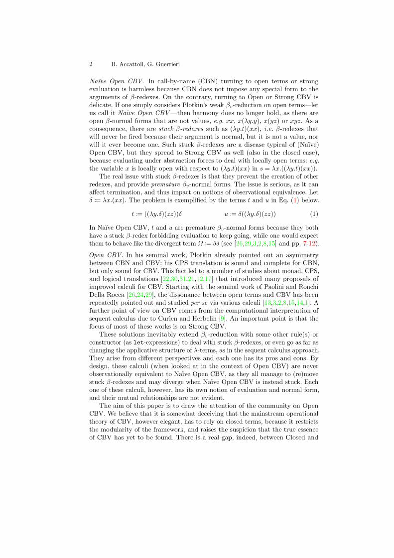
Open Call-by-Value 3: The Shuffling Calculus λsh. The calculus introduced byCarraro and Guerrieri in [8], and here deemed Shuffling Calculus, has the samesyntax of terms as Plotkin’s calculus. Two additional commutation rules help→βv to deal with stuck β-redexes, by shuffling constructors so as to enablecreations of type 1 and 4. As for λvsub, λsh was actually introduced, and thenused in [8,14,15], to study Strong CBV. In Fig. 4 we present its adaptation toOpen CBV, based on balanced contexts, a special notion of evaluation contexts.The reductions →σ[ and →β[v

are non-deterministic and—because of balancedcontexts—can reduce under abstractions, but they are morally weak: they reduceunder a λ only when the λ is applied to an argument. Note that the conditionx /∈ fv(s) (resp. x /∈ fv(v)) in the definition of the shuffling rule 7→σ1

(resp. 7→σ3)

can always be fulfilled by α-conversion.The reduction→σ[ unblocks stuck β-redexes. For instance, consider the terms

t := ((λy.δ)(zz))δ and u := δ((λy.δ)(zz)) where δ := λx.xx (as in Eq. (1), p. 2):t and u are β[v-normal but t →σ[1

(λy.δδ)(zz) →β[v(λy.δδ)(zz) →β[v

. . . and

u→σ[3(λy.δδ)(zz)→β[v

(λx.δδ)(zz)→β[v. . . .


Terms and Values As in Plotkin’s Open CBV (Fig. 1)Balanced Contexts B ::= 〈·〉 | tB | Bt | (λx.B)t

Rule at Top Level Contextual closure((λx.t)u)s 7→σ1 (λx.ts)u, x /∈fv(s) B〈t〉 →σ[1

B〈u〉 if t 7→σ1 u

v((λx.s)u) 7→σ3 (λx.vs)u, x /∈fv(v) B〈t〉 →σ[3B〈u〉 if t 7→σ3 u

(λx.t)v 7→βv txv B〈t〉 →β[vB〈u〉 if t 7→βv u

Reductions →σ[ :=→σ[1∪ →σ[3

, →sh :=→β[v∪ →σ[

Fig. 4. Shuffling λ-calculus λsh

The similar shuffling rules in CBN, better known as Regnier’s σ-rules [28],are contained in CBN β-equivalence, while in Open (and Strong) CBV they aremore interesting, as they are not contained into (i.e. they enrich) βv-equivalence.

The advantage of λsh is with respect to denotational investigations. In [8], λshis indeed used to prove various semantical results in connection to linear logic,resource calculi, and the notion of Taylor expansion due to Ehrhard. In particular,in [8] it has been proved the adequacy of λsh with respect to the relationalmodel induced by linear logic: a by-product of our paper is the extension of thisadequacy result to all incarnations of Open CBV. The drawback of λsh is itstechnical rewriting theory. We summarize some properties of λsh:

Proposition 6 (Basic Properties of λsh, [8]).Proof p. 27

1. Let t, u, s ∈ Λ. If t→β[vu and t→σ[ s then u 6= s.

2. →σ[ is strongly normalizing and (not strongly) confluent.

3. →sh is (not strongly) confluent.

4. Let t ∈ Λ: t is strongly sh-normalizable iff t is sh-normalizable.

In contrast to λfire and λvsub, λsh is not strongly confluent and not all sh-normalizing derivations (if any) from a given term have the same length (consider,for instance, all sh-normalizing derivations from (λy.z)(δ(zz))δ). Nonetheless,normalization and strong normalization still coincide (Prop. 6.4), and Cor. 18in Sect. 3 will show that the discrepancy is encapsulated inside the additionalshuffling rules, as all sh-normalizing derivations from a given term have the samenumber of β[v-steps.

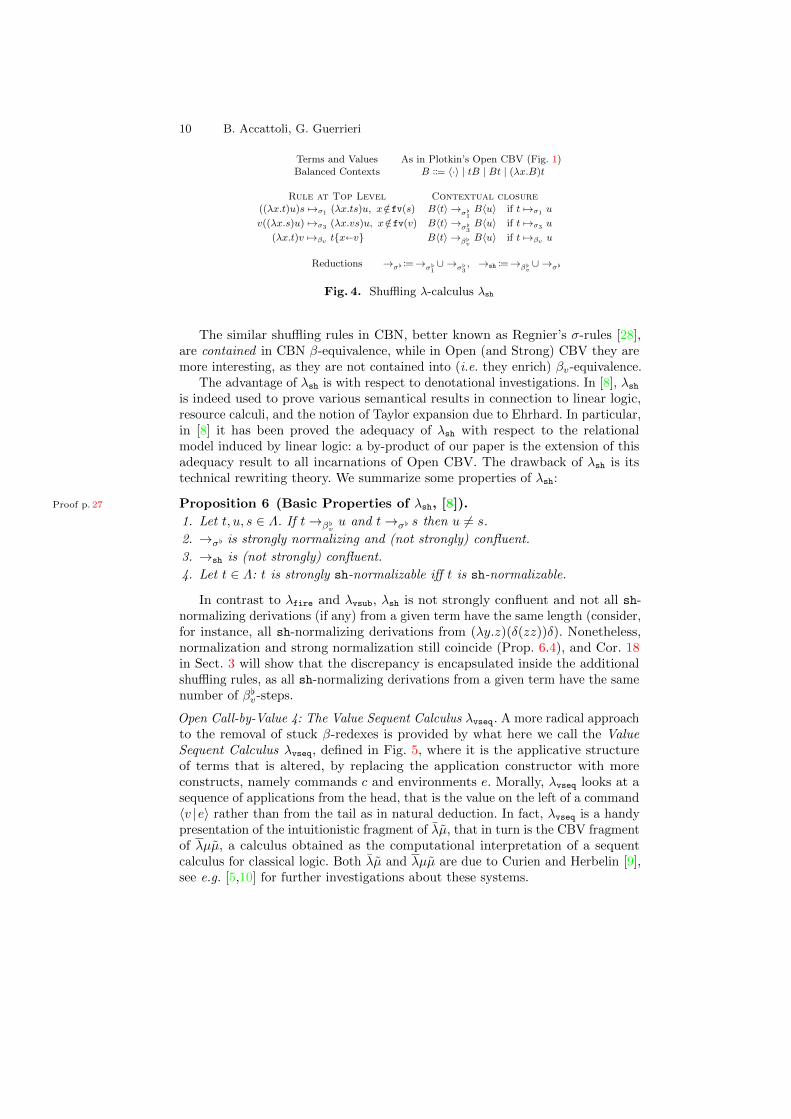
Open Call-by-Value 4: The Value Sequent Calculus λvseq. A more radical approachto the removal of stuck β-redexes is provided by what here we call the ValueSequent Calculus λvseq, defined in Fig. 5, where it is the applicative structureof terms that is altered, by replacing the application constructor with moreconstructs, namely commands c and environments e. Morally, λvseq looks at asequence of applications from the head, that is the value on the left of a command〈v |e〉 rather than from the tail as in natural deduction. In fact, λvseq is a handypresentation of the intuitionistic fragment of λµ, that in turn is the CBV fragmentof λµµ, a calculus obtained as the computational interpretation of a sequentcalculus for classical logic. Both λµ and λµµ are due to Curien and Herbelin [9],see e.g. [5,10] for further investigations about these systems.


Commands c, c′ ::= 〈v |e〉Values v, v′ ::= x | λx.c

Environments e, e′ ::= ε | µx.c | v ·eCommand Evaluation Contexts C ::= 〈·〉 | D〈µx.C〉

Environment Evaluation Contexts D ::= 〈v | 〈·〉〉 | D〈v ·〈·〉〉

Rule at Top Level Contextual closure〈λx.c |v ·e〉 7→λ 〈v |(µx.c)@e〉 C〈c〉 →λ C〈c′〉 if c 7→λ c

′

〈v | µx.c〉 7→µ cxv C〈c〉 →µ C〈c′〉 if c 7→µ c′

Reduction →vseq :=→λ∪ →µ

Fig. 5. Open CBV 4: the λvseq-Calculus

A peculiar trait of the sequent calculus approach is the environment construc-tor µx.c, that is a binder for the free occurrences of x in c. It is often said that itis a sort of explicit substitution—we will see exactly in which sense, in Sect. 4.

The change of the intuitionistic variant λvseq with respect to λµ is that λvseqdoes not need the syntactic category of co-variables α, as there can be only oneof them, that we note ε. From a logic point of view, this is due to the fact thatin intuitionistic sequent calculus, there is neither contraction nor weakening onthe right-hand-side of `. Consequently, the binary abstraction λ(x, α).c of λµ isreplaced by a more traditional unary one λx.c, and substitution on co-variables isreplaced by a notion of appending of environments, defined by mutual inductionon commands and environments as follows:

〈v |e′〉@e := 〈v |e′@e〉 ε@e := e

(v ·e′)@e := v ·(e′@e) (µx.c)@e := µy.(cxy@e) with y /∈ fv(c) ∪ fv(e)

Essentially, c@e is a capture-avoiding substitution of e for the only occurrence ofε in c that is out of all abstractions, which stands for the output of the term. Theappend operation is used in →λ, one of the two rewrite rules of λvseq (Fig. 5).Strong CBV can be obtained by simply extending the grammar of evaluationcontexts to commands under abstractions.

We will provide a translation from λvsub to λvseq, that beyond the terminationequivalence, will show that the switching to the sequent calculus representationis equivalent to a transformation in administrative normal form [30].

The advantage of λvseq is that it avoids both rules at a distance and shufflingrules. The drawback of λvseq is that, syntactically, it requires to step out ofthe λ-calculus. We will show in Sect. 4 how to reformulate it as a fragment ofλvsub, i.e. in natural deduction. However, it will still be necessary to restrict theapplication constructor, thus preventing the natural way of writing λ-terms.

The rewriting of λvseq is very well-behaved, in particular it is strongly confluentand the rules terminates separately.

Proposition 7 (Basic properties of λvseq). Proof p. 30

1. →λ and →µ are strongly normalizing and strongly confluent (separately).

2. →λ and →µ strongly commute.


3. →vseq is strongly confluent, and all vseq-normalizing derivations d from acommand c (if any) have the same length |d|, the same number |d|µ of µ-steps,and the same number |d|λ of λ-steps.

Reducing Open to Closed Call-by-Value: Potential Valuability. Potential valu-ability relates Naıve Open CBV to Closed CBV via a meta-level substitutionclosing open terms: a (possibly open) term t is potentially valuable if there is asubstitution of (closed) values for its free variables, for which it βv-evaluates toa (closed) value. In Naıve Open CBV, potentially valuable terms do not coincidewith normalizable terms because of premature βv-normal forms—as t and u inEq. (1) at p. 2— which are not potentially valuable.

Paolini, Ronchi Della Rocca and, later, Pimentel [26,24,29,25,23] gave severaloperational, logical, and semantical characterizations of potentially valuableterms in Naıve Open CBV. In particular, in [26,29] it is proved that a term ispotentially valuable in Plotkin’s Naıve Open CBV iff its normalizable in λfire.

Potentially valuable terms can be defined for every incarnation of Open CBV:it is enough to update the notions of evaluation and values in the above definitionto the considered calculus. This has been done for λsh in [8], and for λvsub in[3]. For both calculi it has been proved that, in the weak setting, potentiallyvaluable terms coincides with normalizable terms. In [15], it has been provedthat Plotkin’s potentially valuable terms coincide with λsh-potentially valuableterms (which coincide in turn with sh-normalizable terms). Our paper makes afurther step: proving that termination coincides for λfire, λvsub, λsh, and λvseq itimplies that all their notions of potential valuability coincide with Plotkin’s, i.e.there is just one notion of potential valuability.

Open CBV 5, 6, 7, . . . The literature contains many other calculi for CBV,usually presented for Strong CBV and easily adaptable to Open CBV. Some ofthem have let-expressions (avatars of ES) and all of them have rules permutingconstructors, therefore they lie somewhere in between λvsub and λsh. Often, theyhave been developed for other purposes, usually to investigate the relationshipwith monad or CPS translations. Moggi’s equational theory [22] is a classicstandard of reference, known to coincide with that of Sabry and Felleisen [30],Sabry and Wadler [31], Dychoff and Lengrand [12], Herbelin and Zimmerman [17]and Maraist et al’s λlet in [21]. In [3], λvsub modulo ≡ is shown to be terminationequivalent to Herbelin and Zimmerman’s calculus, and to strictly contain itsequational theory, and thus Moggi’s. At the level of rewriting these presentationsof Open CBV are all more involved than those that we consider here. Theirequivalence to our calculi can be shown along the lines of that of λsh with λvsub.

3 Quantitative Equivalence of λfire, λvsub, and λsh

Here we show the equivalence with respect to termination of λfire, λvsub, andλsh, enriched with quantitative information on the number of steps. The resultsare obtained simulating both λfire and λsh into λvsub. In both cases, structuralequivalence ≡ of λvsub plays a role.


Simulating λfire in λvsub. A single βv-step (λx.t)v →βv txv is simulated inλvsub by two steps (Lemma 8.1): (λx.t)v →m t[xv] →e txv, i.e. a m-stepthat creates a ES, and a e-step that turns the ES into the meta-level substitutionperformed by the βv-step. The simulation of an inert step of λfire is insteadtrickier, because in λvsub there is no rule to substitute an inert term, if it is nota variable. The idea is that an inert step (λx.t)i→βi txi is simulated onlyby (λx.t)i →m t[xi], i.e. only by the m-step that creates the ES, and such aES will never be fired—so the simulation is up to the unfolding of substitutionscontaining inert terms (defined right next). Everything works because of the keyproperty of inert terms: they are normal and their substitution cannot createredexes, so it is useless to substitute them.

The unfolding of a vsub-term t is the term t→

obtained from t by turning ESinto meta-level substitutions; it is defined by:

x

→

:= x (tu)

→

:= t

→

u

→

(λx.t)→

:= λx.t

→

(t[xu])

→

:= t

→

xu

→

For all t, u ∈ Λvsub, t ≡ u implies t→

= u

→

. Also, t

→

= t iff t ∈ Λ.In the simulation we are going to show, structural equivalence ≡ plays a role.

It is used to clean the vsub-terms (with ES) obtained by simulation, puttingthem in a canonical form where ES do not appear among other constructors.

A vsub-term is clean if it has the form u[x1i1] . . . [xnin] (with n ∈ N),u ∈ Λ is called the body, and i1, . . . , in ∈ Λ are inert terms. Clearly, any term (asit is without ES) is clean. We first show how to simulate a single fireball step.

Lemma 8 (Simulation of a βf -Step in λvsub). Let t, u ∈ Λ. Proof p. 33

1. If t→βλ u then t→m→eλ u.

2. If t→βi u then t→m≡ s, with s∈Λvsub clean and s

→

= u.

Unfortunately, it is not possible to simulate derivations by iterating Lemma 8,because the starting term t has no ES but the simulation of inert steps introducesES. Therefore, we have to generalize the statement up to the unfolding of ES. Ingeneral, unfolding ES is a dangerous operation with respect to (non-)termination,as it may erase a diverging subterm (e.g. t := x[yδδ] is vsub-divergent andt

→

= x is normal). In our case, however, the simulation produces clean vsub-terms,and so the unfolding is safe because it can only erase inert terms, that cannotcreate, erase, nor carry redexes.

By means of a technical lemma in the appendix we obtain:

Lemma 9 (Projection of a βf -Step on →vsub via Unfolding). Let t be a Proof p. 34

clean vsub-term and u be a term.

1. If t

→

→βλ u then t→m→eλ s, with s∈Λvsub clean and s

→

= u.

2. If t

→

→βi u then t→m≡ s, with s∈Λvsub clean and s

→

= u.

Via Lemma 9 we can now simulate whole derivations. To obtain the termina-tion equivalence, however, we have to work a little bit more. First of all, let uscharacterize the terms in λvsub obtained by projecting normalizing derivations(that always produce a fireball).


Lemma 10. Let t be a clean vsub-term. If t

→

is a fireball, then t is m, eλ- Proof p. 35

normal and its body is a fireball.

Now, a m, eλ-normal form t morally is vsub-normal, as →ey terminates(Prop. 4.1) and it cannot create m, eλ-redexes. The part about creations isbetter expressed as a postponement property.

Lemma 11 (Linear Postponement of →ey). Let t, u ∈ Λvsub. If d : t→∗vsub uProof p. 35

then e : t→∗m,eλ→∗ey u with |e|vsub = |d|vsub, |e|m = |d|m, |e|e = |d|e and |e|eλ≥ |d|eλ .

The next theorem puts all the pieces together.

Theorem 12 (Quantitative Simulation of λfire in λvsub). Let t, u ∈ Λ. IfProof p. 38

d : t→∗βf u then there are s, r∈Λvsub and e : t→∗vsub r such that

1. Qualitative Relationship: r ≡ s, u = s→

= r

→

and s is clean;

2. Quantitative Relationship:

1. Multiplicative Steps: |d|βf = |e|m;

2. Exponential (Abstraction) Steps: |d|βλ = |e|eλ = |e|e.3. Normal Forms: if u is βf -normal then there exists f : r →∗ey q such that q is a

vsub-normal form and |f |ey ≤ |e|m − |e|eλ .

Corollary 13 (Linear Termination Equivalence of λvsub and λfire). LetProof p. 38

t ∈ Λ. There is a βf -normalizing derivation d from t iff there is a vsub-normalizingderivation e from t. Moreover, |d|βf ≤ |e|vsub ≤ 2|d|βf , i.e. they are linearly related.

The statement of Cor. 13 is stronger than it may look at first sight, becauseby strong confluence in both λfire and λvsub, given a term t, if there is a normal-izing derivation from t then there are no diverging derivations from t, and allnormalizing derivations from t have the same length (Prop. 3.3 and Prop. 4.3).

Since the number of steps in λfire is known to be a reasonable cost modelfor Open CBV [1], our result states that also the number of steps in λvsub is areasonable cost model, and moreover that λfire and λvsub are tightly related. Notonly the relationship between the two is linear, but the number of multiplicativesteps in λvsub is exactly the number of steps in λfire (Thm. 12.2). By the way,this is somewhat surprising: in λfire arguments of βf -redexes are required to befireballs, while for m-redexes there are no restrictions on arguments, and yet inevery normalizing derivation from a given term their number coincide.

From Lemma 10 it follows that a clean vsub-normal form is a fireball followedby ES with inert terms. This is a nice description of normal forms for λvsub,inherited from λfire, and a by-product of our study.

Simulating λsh in λvsub. A derivation d : t→∗sh u in λsh is simulated via a projec-tion on multiplicative normal forms in λvsub, i.e. as a derivation m(t)→∗vsub≡ m(u)(for any vsub-term t, its multiplicative and exponential normal forms, denotedby m(t) and e(t) respectively, exist and are unique by Prop. 4). Indeed, a β[v-stepof λsh is simulated in λvsub by a e-step followed by some m-steps to reach the


m-normal form. Shuffling rules →σ[ of λsh are simulated by the structural equiva-lence ≡ of λvsub: applying m(·) to ((λx.t)u)s→σ[1

(λx.(ts))u we obtain exactly an

instance of the axiom ≡@l defining ≡: m(t)[xm(u)]m(s) ≡@l (m(t)m(s))[xm(u)](with the side conditions matching exactly). Similarly,→σ[3

projects to ≡@r or ≡[·](depending on whether v in →σ[3

is a variable or an abstraction). Therefore,

Lemma 14 (Projecting a sh-Step on →vsub≡ via m-nf). Let t, u∈Λ. Proof p. 40

1. If t→σ[ u then m(t) ≡ m(u).

2. If t→β[vu then m(t)→e→∗m m(u).

In contrast to the simulation of λfire in λvsub, here the projection of a singlestep can be extended to derivations without problems, obtaining that the numberof β[v-steps in λsh matches exactly the number of e-steps in λvsub. Additionally,we apply the postponement of ≡ (Lemma 5.2), factoring out the use of ≡ (i.e. ofshuffling rules) without affecting the number of e-steps. So, via Lemma 14 we cannow simulate whole derivations. To obtain the termination equivalence, however,we need the following lemma:

Lemma 15 (Projection Preserves Normal Forms). Let t ∈ Λ. If t is sh- Proof p. 40

normal then m(t) is vsub-normal.

The next theorem puts all the pieces together (for any sh-derivation d, |d|β[vis the number of β[v-steps in d: this notion is well defined by Prop. 6.1).

Theorem 16 (Quantitative Simulation of λsh in λvsub). Let t, u ∈ Λ. If Proof p. 41

d : t→∗sh u then there are s ∈ Λvsub and e : t→∗vsub s such that

1. Qualitative Relationship: s ≡ m(u);

2. Quantitative Relationship (Exponential Steps): |d|β[v = |e|e;3. Normal Form: if u is sh-normal then s and m(u) are vsub-normal.

Corollary 17 (Termination Equivalence of λvsub and λsh). Let t ∈ Λ. Proof p. 41

There is a sh-normalizing derivation d from t iff there is a vsub-normalizingderivation e from t. Moreover, |d|β[v = |e|e.

As for Cor. 13, the claim of Cor. 17 is stronger than it seems, since forboth λvsub and λsh, given a term t, if there is a normalizing derivation from tthen there are no diverging derivations from t (for λvsub it follows from strongconfluence, for λsh is given by Prop. 6.4).

About the quantitative relationship, |d|β[v = |e|e also holds for all normalizingderivations from a given term; for λvsub, it holds by Prop. 4.3; for λsh, it is givenby the following corollary of Thm. 16.

Corollary 18 (Number of β[v-Steps is Invariant). All sh-normalizing deriva- Proof p. 41

tions from t ∈ Λ (if any) have the same number of β[v-steps.

In a way, the quantitative simulation of λsh in λvsub (Thm. 16) “imposesthe good behavior” of λvsub on λsh. The existence of a quantitative invariant insh-normalizing derivations is not obvious, indeed, as λsh is not strongly confluent.


Concerning the cost model, things are subtler for λsh. Note that the rela-tionship between λsh and λvsub uses the number of e-steps, while the cost model(inherited from λfire) is the number of m-steps. Do e-steps provide a reasonablecost model? Probably not, because there is a family of terms that evaluate inexponentially more m-steps than e-steps. Details are left to a longer version.

4 Quantitative Equivalence of λvsub and λvseq, via λvsubk

The quantitative termination equivalence of λvsub and λvseq is shown in two steps:first, we identify a sub-calculus λvsubk of λvsub equivalent to the whole of λvsub,and then show that λvsubk and λvseq are equivalent (actually isomorphic).

Equivalence of λvsubk and λvsub. The kernel λvsubk of λvsub is the sublanguageof λvsub obtained by replacing the application constructor tu with the restrictedform tv where the right subterm can only be a value v—i.e., λvsubk is the languageof so-called administrative normal form [30] of λvsub. The rewriting rules are thesame of vsub. It is easy to see that vsubk is stable by reduction. For lack ofspace, more details about vsubk have been moved to Appendix B.3 (page 42).

The translation (·)+ of λvsub into λvsubk , which simply places the argument ofan application into an ES, is defined by (note that fv(t) = fv(t+) for all t∈Λvsub):

x+ := x (tu)+ := (t+x)[xu+] where x /∈ fv(t) ∪ fv(u)

(λx.t)+ := λx.t+ t[xu]+ := t+[xu+]

Lemma 19 (Simulation). Let t, u ∈ Λvsub.Proof p. 42

1. Multiplicative: if t→m u then t+ →m→ey≡ u+;

2. Exponential: if t→eλ u then t+ →eλ u+, and if t→ey u then t+ →ey u

+.

3. Structural Equivalence: t ≡ u implies t+ ≡ u+.

Theorem 20 (Quantitative Simulation of λvsub in λvsubk). Let t, u ∈ Λvsub.Proof p. 44

If d : t→∗vsub u then there are s ∈ Λvsubk and e : t+ →∗vsubk s such that

1. Qualitative Relationship: s ≡ u+;

2. Quantitative Relationship:1. Multiplicative Steps: |e|m = |d|m;

2. Exponential Steps: |e|eλ = |d|eλ and |e|ey = |d|ey + |d|m;

3. Normal Form: if u is normal then s is m-normal and e(s) is normal.

Corollary 21 (Linear Termination Equivalence of λvsub and λvsubk). Lett ∈ Λvsub. There exists a vsub-normalizing derivation d from t iff there exists aProof p. 44

vsubk-normalizing derivation e from t+. Moreover, |d|vsub ≤ |e|vsubk ≤ 3|d|vsub.

Equivalence of λvsubk and λvseq. The translation · of λvsubk into λvseq is definedas follows, and relies on an auxiliary translation (·)• of values:

x• := x (λx.t)• := λx.tv := 〈v |ε〉 tv := t@(v• ·ε) t[xu] := u@µx.t


It is not hard to see that λvsubk and λvseq are actually isomorphic, where the con-verse translation (·), that maps values and commands to terms, and environmentsto evaluation contexts, is given by:

x := x ε := 〈·〉〈v |e〉 := e〈v〉(λx.c) := λx.c (v ·e) := e〈〈·〉v〉 (µx.c) := c[x〈·〉]

We follow, however, the same structure of the other weaker equivalences.

Lemma 22 (Simulation of →vsubk by →vseq). Let t and u be vsubk-terms. Proof p. 46

1. Multiplicative: if t→m u then t→λ u.

2. Exponential: if t→e u then t→µ u.

Theorem 23 (Quantitative Simulation of λvsubk in λvseq). Let t and u be Proof p. 47

vsubk-terms. If d : t→∗vsubk u then there is e : t→∗vseq u such that

1. Multiplicative Steps: |d|m = |e|λ (the number λ-steps in e);

2. Exponential Steps: |d|e = |e|µ (the number µ-steps in e), so |d|vsubk = |e|vseq;

3. Normal Form: if u is vsubk-normal then u is vseq-normal.

Corollary 24 (Linear Termination Equivalence of λvsubk and λvseq). Lett be a vsubk-term. There is a vsubk-normalizing derivation d from t iff there is Proof p. 47

a vseq-normalizing derivation e from t. Moreover, |d|vsubk = |e|vseq, |d|e = |e|µand |d|m = |e|λ.

Structural Equivalence for λvseq. The equivalence of λvsub and λvsubk relies onthe structural equivalence ≡ of λvsub, so it is natural to wonder how does ≡look on λvseq. The structural equivalence l of λvseq is defined as the closure byevaluation contexts of the following axiom

D〈µx.D′〈µy.c〉〉 lµµ D′〈µy.D〈µx.c〉〉 where x /∈ fv(D′) and y /∈ fv(D).

As expected, l has, with respect to λvseq, all the properties of≡ (see Lemma 5).They are formally stated in the appendix, for lack of space.

References

1. Accattoli, B., Sacerdoti Coen, C.: On the Relative Usefulness of Fireballs. In: LICS2015. pp. 141–155 (2015)

2. Accattoli, B.: Proof nets and the call-by-value λ-calculus. Theor. Comput. Sci. 606,2–24 (2015)

3. Accattoli, B., Paolini, L.: Call-by-Value Solvability, revisited. In: FLOPS. pp. 4–16(2012)

4. Accattoli, B., Sacerdoti Coen, C.: On the Value of Variables. In: WoLLIC 2014. pp.36–50 (2014)

5. Ariola, Z.M., Bohannon, A., Sabry, A.: Sequent calculi and abstract machines. ACMTrans. Program. Lang. Syst. 31(4) (2009)

6. Barendregt, H.P.: The Lambda Calculus – Its Syntax and Semantics, vol. 103.North-Holland (1984)


7. Blelloch, G.E., Greiner, J.: Parallelism in Sequential Functional Languages. In:FPCA. pp. 226–237 (1995)

8. Carraro, A., Guerrieri, G.: A Semantical and Operational Account of Call-by-ValueSolvability. In: FOSSACS 2014. pp. 103–118 (2014)

9. Curien, P.L., Herbelin, H.: The duality of computation. In: ICFP. pp. 233–243(2000)

10. Curien, P., Munch-Maccagnoni, G.: The Duality of Computation under Focus. In:6th IFIP, TCS 2010. Proceedings. vol. 323, pp. 165–181. Springer (2010)

11. Dal Lago, U., Martini, S.: The weak lambda calculus as a reasonable machine.Theor. Comput. Sci. 398(1-3), 32–50 (2008)

12. Dyckhoff, R., Lengrand, S.: Call-by-Value lambda-calculus and LJQ. J. Log. Comput.17(6), 1109–1134 (2007)

13. Gregoire, B., Leroy, X.: A compiled implementation of strong reduction. In: (ICFP’02). pp. 235–246 (2002)

14. Guerrieri, G.: Head reduction and normalization in a call-by-value lambda-calculus.In: WPTE 2015. pp. 3–17 (2015)

15. Guerrieri, G., Paolini, L., Ronchi Della Rocca, S.: Standardization of a Call-By-ValueLambda-Calculus. In: TLCA 2015. pp. 211–225 (2015)

16. Herbelin, H.: C’est maintenant qu’on calcule: au cœur de la dualite (2005), Habili-tation thesis

17. Herbelin, H., Zimmermann, S.: An operational account of Call-by-Value Minimaland Classical λ-calculus in Natural Deduction form. In: TLCA. pp. 142–156 (2009)

18. Jones, N.D., Gomard, C.K., Sestoft, P.: Partial Evaluation and Automatic ProgramGeneration. Prentice-Hall, Inc., Upper Saddle River, NJ, USA (1993)

19. Lassen, S.: Eager Normal Form Bisimulation. In: LICS 2005. pp. 345–354 (2005)20. Levy, J.J.: Reductions correctes et optimales dans le lambda-calcul. These d’Etat,

Univ. Paris VII, France (1978)21. Maraist, J., Odersky, M., Turner, D.N., Wadler, P.: Call-by-name, Call-by-value,

Call-by-need and the Linear λ-Calculus. TCS 228(1-2), 175–210 (1999)22. Moggi, E.: Computational λ-Calculus and Monads. In: LICS ’89. pp. 14–23 (1989)23. Paolini, L., Pimentel, E., Ronchi Della Rocca, S.: Strong Normalization from an

unusual point of view. Theor. Comp. Science 412(20), 1903–1915 (2011)24. Paolini, L.: Call-by-Value Separability and Computability. In: ICTCS. pp. 74–89

(2002)25. Paolini, L., Pimentel, E., Ronchi Della Rocca, S.: Lazy strong normalization. In:

ITRS ’04. Electronic Notes in Theoretical Computer Science, vol. 136C, pp. 103–116(2005)

26. Paolini, L., Ronchi Della Rocca, S.: Call-by-value Solvability. ITA 33(6), 507–534(1999)

27. Plotkin, G.D.: Call-by-Name, Call-by-Value and the lambda-Calculus. Theor. Com-put. Sci. 1(2), 125–159 (1975)

28. Regnier, L.: Une equivalence sur les lambda-termes. TCS 2(126), 281–292 (1994)29. Ronchi Della Rocca, S., Paolini, L.: The Parametric λ-Calculus. Springer Berlin

Heidelberg (2004)30. Sabry, A., Felleisen, M.: Reasoning about Programs in Continuation-Passing Style.

Lisp and Symbolic Computation 6(3-4), 289–360 (1993)31. Sabry, A., Wadler, P.: A Reflection on Call-by-Value. ACM Trans. Program. Lang.

Syst. 19(6), 916–941 (1997)32. Sands, D., Gustavsson, J., Moran, A.: Lambda Calculi and Linear Speedups. In: The

Essence of Computation, Complexity, Analysis, Transformation. Essays Dedicatedto Neil D. Jones. pp. 60–84 (2002)

Technical Appendix

A Rewriting Theory: Definitions, Notations, and BasicResults

Given a binary relation →r on a set I, the reflexive-transitive (resp. reflexive;transitive; reflexive-transitive and symmetric) closure of →r is denoted by →∗(resp. →=

r ; →+r ; 'r). The transpose of →r is denoted by r←. A (r-)derivation d

from t to u, denoted by d : t→∗r u, is a finite sequence (ti)0≤i≤n of elements of I(with n ∈ N) s.t. t = t0, u = tn and ti →r ti+1 for all 1 ≤ i < n;

The number of r-steps of a derivation d, i.e. its length, is denoted by |d|r := n,or simply |d|. If→r =→1∪ →2 with→1∩ →2 = ∅, |d|i is the number of→i-stepsin d, for i = 1, 2. We say that:

– t∈I is r-normal or a r-normal form if t 6→r u for all u∈I; u ∈ I is a r-normalform of t if u is r-normal and t→∗r u;

– t ∈ I is r-normalizable if there is a r-normal u ∈ I s.t. t→∗r u; t is stronglyr-normalizable if there is no infinite sequence (ti)i∈N s.t. t0 = t and ti →r ti+1;

– a r-derivation d : t→∗r u is (r-)normalizing if u is r-normal;– →r is strongly normalizing if all t∈I is strongly r-normalizable;– →r is strongly confluent if, for all t, u, s ∈I s.t. s r← t→r u and u 6= s, there

is r ∈ I s.t. s→r r r← u; →r is confluent if →∗r is strongly confluent.

Let →1,→2⊆ I × I. Composition of relations is denoted by juxtaposition: forinstance, t →1→2 u means that there is s ∈ I s.t. t →1 s →2 u; for any n ∈ N,t→n

1 u means that there is a →1-derivation with length n (t = u for n = 0). Wesay that→1 and→2 strongly commute if, for any t, u, s ∈ I s.t. u 1← t→2 s, onehas u 6= s and there is r ∈ I s.t. u→2 r 1← s. Note that if →1 and →2 stronglycommute and →=→1∪ →2, then for any derivation d : t→∗ u the sizes |d|1 and|d|2 are uniquely determined.

The following proposition collects some basic and well-known results ofrewriting theory.

Proposition 25. Let →r be a binary relation on a set I.

1. If →r is confluent then:(a) every r-normalizable term has a unique r-normal form;(b) for all t, u ∈ I, t 'r u iff there is s ∈ I s.t. t→∗r s ∗r← u.

2. If →r is strongly confluent then →r is confluent and, for any t ∈ I, one has:(a) all normalizing r-derivations from t have the same length;(b) t is strongly r-normalizable if and only if t is r-normalizable.

As all incarnations of Open CBV we consider are confluent, the use ofProp. 25.1 is left implicit.

For λfire and λvsub, we use Prop. 25.2 and the following more informativeversion of Hindley–Rosen Lemma, whose proof is just a more accurate reading ofthe proof in [6, Prop. 3.3.5.(i)]:


Lemma 26 (Strong Hindley–Rosen). Let→=→1 ∪ →2 be a binary relationon a set I s.t.→1 and→2 are strongly confluent. If→1 and→2 strongly commute,then → is strongly confluent and, for any t ∈ I and any normalizing derivationsd and e from t, one has |d| = |e|, |d|1 = |e|1 and |d|2 = |e|2.

B Omitted Proofs

B.1 Proofs of Section 2 (Incarnations of Open Call-by-Value)

Naıve Open CBV: Plotkin’s Calculus λPlot

Remark 27. Since →βv does not reduce under λ’s, any value is βv-normal, andso βy-normal and βλ-normal, as →βy ,→βλ ⊆→βv .

Proposition 1. →βy , →βλ and →βv are strongly confluent.See p. 5

Proof. We prove that →βv is strongly confluent. The proofs that →βy and →βλ

are strongly confluent are perfectly analogous.So, we prove, by induction on t, that if t→βv u and t→βv s with u 6= s, then

there exists t′ such that u→βv t′ and s→βv t

′.Observe that neither t→βv u nor t→βv s can be a step at the root: indeed, if

t := (λx.r)v →βv rxv =: u and t→βv s (or if t := (λx.r)v →βv rxv =: sand t→βv u), then u = s since λx.r and v are βv-normal by Remark 27; but thiscontradicts the hypothesis u 6= s. So, according to the definition of t→βv u andt→βv s, there are only four cases.

– Application Left for t →βv u and t →βv s, i.e. t = rq →βv pq = u andt = rq →βv mq = s with r →βv p and r →βv m. By the hypothesis u 6= s itfollows that p 6= m. By i.h., there exists r′ such that p→βv r

′ and m→βv r′.

So, setting t′ = r′q, one has u = pq →βv t′ and s = mq →βv t

′.– Application Right for t →βv u and t →βv s, i.e. t = rq →βv rp = u andt = rq →βv rm = s with q →βv p and q →βv m. From the hypothesis u 6= s itfollows that p 6= m. By i.h., there exists q′ such that p→βv q

′ and m→βv q′.

So, setting t′ = rq′, one has u = rp→βv t′ and s = rm→βv t

′.– Application Left for t →βv u and Application Right for t →βv s, i.e. t =rq →βv pq = u and t = rq →βv rm = s with r →βv p and q →βv m. So,setting t′ = pm, one has u = pq →βv t

′ and s = rm→βv t′.

– Application Right for t →βv u and Application Left for t →βv s, i.e. t =rq →βv rp = u and t = rq →βv mq = s with q →βv p and r →βv m. So,setting t′ = mp, one has u = rp→βv t

′ and s = mq →βv t′.

Open CBV 1: the Fireball Calculus λfire

Lemma 28 (Values and inert terms are βf -normal).

1. Every value is βf -normal.2. Every inert term is βf -normal.

Proof.


1. Immediate, since →βf does not reduce under λ’s.2. By induction on the definition of inert term i.

– If i = x then i is obviously βf -normal.– If i = i′λx.t then i′ and λx.t are βf -normal by i.h. and Lemma 28.1

respectively, besides i′ is not an abstraction, so i is βf -normal.– Finally, if i = i′i′′ then i′ and i′′ are βf -normal by i.h., moreover i′ is not

an abstraction, hence i is βf -normal.

Proposition 2 (Open Harmony). Let t ∈ Λ: t is βf -normal iff t is a fireball. See p. 6

Proof.

⇒: Proof by induction on t ∈ Λ. If t is a value then t is a fireball.Otherwise t = us for some terms u and s. Since t is βf -normal, then u and sare βf -normal, and either u is not an abstraction or s is not a fireball. Byinduction hypothesis, u and s are fireballs. Summing up, u is either a variableor an inert term, and s is a fireball, therefore t = us is an inert term andhence a fireball.

⇐: By hypothesis, t is either a value or an inert term. If t is a value, then itis βf -normal by Lemma 28.1. Otherwise t is an inert term and then it isβf -normal by Lemma 28.2.

Lemma 29. For every t, t′ ∈ Λ, if t→βi t′ then t 6= t′.

Proof. By induction on t ∈ Λ. According to the definition of t→βi t′, there are

three cases.

– Step at the root, i.e. t = (λx.u)i →βi uxi = t′: then, since i is not anabstraction, necessarily t = (λx.u)i 6= uxi = t′.

– Application Left, i.e. t = us→βi u′s = t′ with u→βi u

′: by i.h., u 6= u′ andhence t = us 6= u′s = t′.

– Application Right, i.e. t = us→βi us′ = t′ with s→βi s

′: by i.h., s 6= s′ andhence t = us 6= us′ = t′.

Proposition 3 (Basic Properties of λfire). See p. 7

1. →βi is strongly normalizing and strongly confluent.2. →βλ and →βi strongly commute.3. →βf is strongly confluent, and all βf -normalizing derivations d from t ∈ Λ

(if any) have the same length |d|βf , the same number |d|βλ of βλ-steps, andthe same number |d|βi of βi-steps.

Proof.

1. Strong normalization of →βi follows from general termination propertiesin the ordinary (i.e. pure, strong, and call-by-name) λ-calculus, as we nowexplain. Since βi-steps do not substitute abstractions, they can only causecreations of type 1, according to Levy’s classification of creations of β-redexes[20]. Then βi-derivations can be seen as special cases of m-developments (see


Accattoli, B., Kesner, D., The Permutative λ-Calculus. In: LPAR. pp. 23-36,2012), in turn a special case of more famous superdevelopments, i.e. reductionsequences reducing only (residuals of) redexes in the original term pluscreations of type 1 (m-developments) or type 1 and 2 (superdevelopments).Both m-developments and superdevelopments always terminate. Therefore,→βi is strongly normalizing.

Now, we prove that →βi is strongly confluent, that is if t→βi u and t→βi swith u 6= s, then there exists t′ ∈ Λ such that u →βi t

′ and s →βi t′. The

proof is by induction on t ∈ Λ.Observe that neither t→βi u nor t→βi s can be a step at the root: indeed, ift := (λx.r)i 7→βi rxi := u and t→βi s (or if t := (λx.r)i 7→βi rxi =: sand t→βi u), then u = s since λx.r and i are βi-normal by Lemmas 28.1-2(as →βi ⊆→βf ); but this contradicts the hypothesis u 6= s. So, according tothe definition of t→βi u and t→βi s, there are only four cases.

– Application Left for t →βi u and t →βi s, i.e. t = rq →βi pq = u andt = rq →βi mq = s with r →βi p and r →βi m. By the hypothesis u 6= sit follows that p 6= m. By i.h., there exists r′ such that p →βi r

′ andm→βi r

′. So, setting t′ = r′q, one has u = pq →βi t′ and s = mq →βi t

′.– Application Right for t →βi u and t →βi s, i.e. t = rq →βi rp = u andt = rq →βi rm = s with q →βi p and q →βi m. By the hypothesis u 6= sit follows that p 6= m. By i.h., there exists q′ such that p →βi q

′ andm→βi q

′. So, setting t′ = rq′, one has u = rp→βi t′ and s = rm→βi t

′.– Application Left for t →βi u and Application Right for t →βi s, i.e.t = rq →βi pq = u and t = rq →βi rm = s with r →βi p and q →βi m.So, setting t′ = pm, one has u = pq →βi t

′ and s = rm→βi t′.

– Application Right for t →βi u and Application Left for t →βi s, i.e.t = rq →βi rp = u and t = rq →βi mq = s with q →βi p and r →βi m.So, setting t′ = mp, one has u = rp→βi t

′ and s = mq →βi t′.

2. We prove, by induction on t ∈ Λ, that if t →βλ u and t →βi s, then u 6= sand there is t′∈ Λ such that u→βi t

′ and s→βλ t′.

Observe that neither t→βλ u nor t→βi s can be a step at the root: indeed,if t := (λx.r)λy.q 7→βλ rxλy.q =: u (resp. t := (λx.r)i 7→βi rxi =: s)then λy.q is not a inert term (resp. i is not an abstraction), moreover λx.rand λy.q (resp. i) are βi-normal (resp. βλ-normal) by Prop. 2, as →βi ⊆→βf (resp. →βλ ⊆→βf ); therefore, t is βi-normal (resp. βλ-normal) but thiscontradicts the hypothesis t →βi s (resp. t →βλ u). So, according to thedefinitions of t→βλ u and t→βi s, there are only four cases.

– Application Left for both t →βλ u and t →βi s, i.e. t := rq →βλ pq =: uand t := rq →βi mq =: s with r →βλ p and r →βi m. By i.h., p 6= m andthere exists r′ such that p→βi r

′ and m→βλ r′. So, u 6= s and, setting

t′ := r′q, one has u = pq →βi t′βλ← mq = s.

– Application Right for both t→βλ u and t→βi s, i.e. t := rq →βλ rp =: uand t := rq →βi rm =: s with q →βλ p and q →βi m. By i.h., p 6= m andthere exists q′ such that p→βi q

′ and m→βλ q′. So, u 6= s and, setting

t′ := rq′, one has u = rp→βi t′βλ← rm = s.


– Application Left for t →βλ u and Application Right for t →βi s, i.e.t := rq →βλ pq = u and t = rq →βi rm =: s with r →βλ p and q →βi m.By Lemma 29, q 6= m and hence u = pq 6= rm = s. Setting t′ := pm, onehas u = pq →βi t

′βλ← rm = s.

– Application Right for t →βλ u and Application Left for t →βi s, i.e.t := rq →βλ rp =: u and t = rq →βi mq = s with q →βλ p and r →βi m.By Lemma 29, r 6= m and hence u = rp 6= mq = s. Setting t′ := mp, onehas u = rp→βi t

′βλ← mq = s.

3. It follows immediately from strong confluence of →βλ (Prop. 1.1) and →βi

(Prop. 3.1), the strong commutation of→βλ and→βi (Prop. 3.2), and Hindley-Rosen (Lemma 26).

Open CBV 2: the Value Substitution Calculus λvsub

Proposition 4 (Basic Properties of λvsub, [3]). See p. 8

1. →m and →e are strongly normalizing (separately).2. →m and →e are strongly confluent (separately).3. →m and →e strongly commute.4. →vsub is strongly confluent, and all vsub-normalizing derivations d from

t ∈ Λvsub (if any) have the same length |d|vsub, the same number |d|e ofe-steps, and the same number |d|e of m-steps.

5. Let t∈Λ. For any vsub-derivation d from t, |d|e ≤ |d|m.

Proof. The statements of Prop. 4 are a refinement of some results proved in [3],where →vsub is denoted by →w.

1. In [3, Lemma 3] it has been proved that →dB and →vs are strongly nor-malizing, separately. Since →m⊆→dB and →e⊆→vs (→dB and →vs are justthe extensions of →m and →e, respectively, obtained by allowing reductionsunder λ’s), one has that →m and →e are strongly normalizing, separately.

2. We prove that →m is strongly confluent, i.e. if u m← t→m s with u 6= s thenthere exists t′ ∈ Λvsub such that u→m t′ m← s. The proof is by induction onthe definition of →m. Since there t→m s 6= u and the reduction →m is weak,there are only eight cases:– Step at the Root for t →m u and Application Right for t →m s, i.e.t := L〈λx.q〉r 7→m L〈q[xr]〉 =: u and t 7→mL〈λx.q〉r′=: s with r→m r

′:then, u→mL〈q[xr′]〉m← s;

– Step at the Root for t→m u and Application Left for t→m s, i.e., for somen > 0, t := (λx.q)[x1t1] . . . [xntn]r 7→m q[xr][x1t1] . . . [xntn] =: uwhereas t →m (λx.q)[x1t1] . . . [xjt′j ] . . . [xntn]r =: s with tj →m t′jfor some 1 ≤ j ≤ n: then,

u→m q[xr][x1t1] . . . [xjt′j ] . . . [xntn] m← s;

– Application Left for t →m u and Application Right for t →m s, i.e.t := rq →m r′q =: u and t→m rq′ =: s with r →m r′ and q →m q′: then,u→m r′q′m← s;


– Application Left for both t →m u and t →m s, i.e. t := rq →m r′q =: uand t→m r′′q =: s with r′ m← r →m r′′: by i.h., there exists r0 ∈ Λvsub

such that r′ →m r0 m← r′′, hence u→m r0q m← s;– Application Right for both t→m u and t→m s, i.e. t := qr →m qr′ =: u

and t→m qr′′ =: s with r′ m← r →m r′′: by i.h., there exists r0 ∈ Λvsub

such that r′ →m r0 m← r′′, hence u→m qr0 m← s;– ES Left for t →m u and ES Right for t →m s, i.e. t := r[xq] →m

r′[xq] =: u and t →m r[xq′] =: s with r →m r′ and q →m q′: then,u→m r′[xq′]m← s;

– ES Left for both t→m u and t→m s, i.e. t := r[xq]→m r′[xq] =: u andt→m r′′[xq] =: s with r′ m← r →m r′′: by i.h., there exists r0 ∈ Λvsub

such that r′ →m r0 m← r′′, hence u→m r0[xq] m← s;– ES Right for both t→m u and t→m s, i.e. t := q[xr]→m q[xr′] =: u

and t →m q[xr′′] =: s with r′ m← r →m r′′: by i.h., there existsr0 ∈ Λvsub such that r′ →m r0 m← r′′, hence u→m q[xr0] m← s.

We prove that →e is strongly confluent, i.e. if u e← t→e s with u 6= s thenthere exists r ∈ Λvsub such that u→e t

′e← s. The proof is by induction on

the definition of →e. Since there t→e s 6= u and the reduction →e is weak,there are only eight cases:– Step at the Root for t→eu and ES Left for t→e s, i.e. t := r[xL〈v〉] 7→e

L〈rxv〉 =: u and t 7→e r′[xL〈v〉] =: s with r →e r

′: then, u →e

L〈r′[xv]〉 e← s;– Step at the Root for t →e u and ES Right for t →e s, i.e., for somen > 0, t := r[xv[x1t1] . . . [xntn]] 7→e rxv[x1t1] . . . [xntn] =: uwhereas t→e r[xv[x1t1] . . . [xjt′j ] . . . [xntn]] =: s with tj →e t

′j for

some 1 ≤ j ≤ n: then,

u→e rxv[x1t1] . . . [xjt′j ] . . . [xntn] e← s;

– Application Left for t →e u and Application Right for t →e s, i.e. t :=rq →e r

′q =: u and t →e rq′ =: s with r →e r

′ and q →e q′: then,

u→e r′q′ e← s;

– Application Left for both t→e u and t→e s, i.e. t := rq →e r′q =: u and

t →e r′′q =: s with r′ e← r →e r

′′: by i.h., there exists r0 ∈ Λvsub suchthat r′ →e r0 e← r′′, hence u→e r0q e← s;

– Application Right for both t →e u and t →e s, i.e. t := qr →e qr′ =: u

and t →e qr′′ =: s with r′ e← r →e r

′′: by i.h., there exists r0 ∈ Λvsub

such that r′ →e r0 e← r′′, hence u→e qr0 e← s;– ES Left for t →e u and ES Right for t →e s, i.e. t := r[xq] →e

r′[xq] =: u and t →e r[xq′] =: s with r →e r′ and q →e q

′: then,u→e r

′[xq′] e← s;– ES Left for both t→e u and t→e s, i.e. t := r[xq]→e r

′[xq] =: u andt →e r

′′[xq] =: s with r′ e← r →e r′′: by i.h., there exists r0 ∈ Λvsub

such that r′ →e r0 e← r′′, hence u→e r0[xq] e← s;– ES Right for both t →e u and t →e s, i.e. t := q[xr] →e q[xr′] =: u

and t→e q[xr′′] =: s with r′ e← r →e r′′: by i.h., there exists r0 ∈ Λvsub

such that r′ →e r0 e← r′′, hence u→e q[xr0] e← s.


Note that in [3, Lemma 11] it has just been proved the strong confluence of→vsub, not of →m or →e.

3. We show that→e and→m strongly commute, i.e. if u e← t→m s, then u 6= sand there is t′ ∈ Λvsub such that u →m t′ e← s. The proof is by inductionon the definition of t→e u. The proof that u 6= s is left to the reader. Sincethe →e and →m cannot reduce under λ’s, all vsub-values are m-normal ande-normal. So, there are the following cases.– Step at the Root for t→e u and ES Left for t→m s, i.e. t := r[zL〈v〉]→e

L〈rzv〉 =: u and t →m r′[zL〈v〉] =: s with r →m r′: then u →m

L〈r′zv〉 e← u;– Step at the Root for t→e u and ES Right for t→m s, i.e.

t := r[zv[x1t1] . . . [xntn]]

→e rzv[x1t1] . . . [xntn] =: u

and t→m r[zv[x1t1] . . . [xjt′j ] . . . [xntn]] =: s for some n > 0, andtj →m t′j for some 1 ≤ j ≤ n: then, u→m rzv[x1t1] . . . [xjt′j ] . . . [xntn] e← s;

– Application Left for t →e u and Application Right for t →m s, i.e.t := rq →e r

′q =: u and t →m rq′ =: s with r →e r′ and q →m q′: then,

t→m r′q′ e← u;– Application Left for both t→e u and t→m s, i.e. t := rq →e r

′q =: u andt →m r′′q =: s with r′ e← r →m r′′: by i.h., there exists p ∈ Λvsub suchthat r′ →m p e← r′′, hence u→m pq e← s;

– Application Left for t →e u and Step at the Root for t →m s, i.e. t :=(λx.q)[x1t1] . . . [xntn]r →e (λx.q)[x1t1] . . . [xjt′j ] . . . [xntn]r =: uwith n > 0 and tj →e t

′j for some 1 ≤ j ≤ n, and t→m q[xr][x1t1] . . . [xntn] =:

s: then,

u→m q[xr][x1t1] . . . [xjt′j ] . . . [xntn] e← s;

– Application Right for t →e u and Application Left for t →m s, i.e.t := qr →e qr

′ =: u and t →m q′r =: s with r →e r′ and q →m q′: then,

u→m q′r′ e← s;– Application Right for both t →e u and t →m s, i.e. t := qr →e qr

′ =: uand t →m qr′′ =: s with r′ e← r →m r′′: by i.h., there exists p ∈ Λvsub

such that r′ →m p e← r′′, hence u→m qp e← s;– Application Right for t →e u and Step at the Root for t →m s, i.e.t := L〈λx.q〉r →e L〈λx.q〉r′ =: u with r →e r

′, and t→m L〈q[xr]〉 =: s:then, u→m L〈q[xr′]〉 e← s;

– ES Left for t →e u and ES Right for t →m s, i.e. t := r[xq] →e

r′[xq] =: u and t →m r[xq′] =: s with r →e r′ and q →m q′: then,

u→m r′[xq′] e← s;– ES Left for both t→e u and t→m s, i.e. t := r[xq]→e r

′[xq] =: u andt →m r′′[xq] =: s with r′ e← r →m r′′: by i.h.,there exists p ∈ Λvsub

such that r′ →m p e← r′′, hence u→m p[xq] e← s;– ES Right for t →e u and ES Left for t →m s, i.e. t := q[xr] →e

q[xr′] =: u and t →m q′[xr] =: s with r →e r′ and q →m q′: then,

u→m q′[xr′] e← s;


– ES Right for both t →e u and t →m s, i.e. t := q[xr] →e q[xr′] =: uand t→m q[xr′′] =: s with r e← r′ →m r′′: by i.h., there exists p ∈ Λvsub

such that r →m p e← r′′, hence u→m q[xp] e← s.4. It follows immediately from strong confluence of →m and →e (Prop. 4.1),

strong commutation of→m and→e (Prop. 4.2) and Hindley-Rosen (Lemma 26).A different proof of the strong confluence of →vsub (without informationabout the number of steps) is in [3, Lemma 11].

5. The intuition behind the proof is that any m-step creates a new ES, anye-step erases an ES. Formally, let u∈Λvsub such that d : t→∗vsub u. We proveby induction on |d|vsub ∈ N that |d|e = |d|m−|u|ES (where |u|ES is the numberof ES in u) and any vsub-value that is a subterm of u is a value (withoutES).If |d|vsub = 0, then u = t ∈ Λ, then we can conclude.Suppose |d|vsub > 0: then, d is the concatenation of d′ : t →∗vsub s ands →vsub u, for some s ∈ Λvsub. By i.h., |d′|e = |d′|m − |s|ES and that everyvsub-value that is a subterm of s is a value (without ES). There are twocases:– s := E〈r[xL〈v〉]〉 →e E〈L〈rxv〉〉 =: u, then |d|m = |d′|m and |s|ES =|u|ES +1, since |v|ES = 0 by i.h.; therefore |d|e = |d′|e +1 = |d′|m−|s|ES +1 = |d|m − |u|ES and any vsub-value that is a subterm of u is a value(without ES).

– s := E〈L〈λx.r〉q〉 →m E〈L〈r[xq]〉〉 =: u, then |u|ES = |s|ES + 1 and|d|m = |d′|m + 1, therefore |d|e = |d′|e = |d′|m − |s|ES = |d|m − |u|ES.Moreover, the new occurrence of ES [xq] in u cannot be under thescope of a λ, otherwise the redex in s which is fired in the m-step wouldbe under the scope of a λ, but this is impossible since →m is a weakreduction. So, any vsub-value that is a subterm of u is a value (withoutES).

Open CBV 3: the Shuffling Calculus λsh

Definition 30 (Occurrences). For all t ∈ Λ, let [t]λ be the number of occur-rences of λ in t, and [t]x be the number of free occurrences of the variable x in t,and subu(t) be the number of occurrences in t of the term u.

Remark 31. Since→β[vand→σ[ do not reduce under λ’s without argument, every

value is β[v-normal and σ[-normal, and hence sh-normal.

Remark 32. The reduction →σ[ is just the closure under balanced contexts ofthe binary relation 7→σ = 7→σ1

∪ 7→σ3on Λ (see definitions in Fig. 4).

Lemma 33. Let t, t′ ∈ Λ.

1. For every value v, if t→σ[ t′ then (λx.t′)v 6= txv.

2. If t→σ[ t′ then t 6= t′.

3. For every value v, one has txv 6= λx.tv.


Proof.

1. By induction on the definition of t→σ[ t′, using Remark 32.

2. In [8, Proposition 2] it has been proved that there exists a size #: Λ → Nsuch that if t →σ t

′ then #(t) > #(t′), where →σ is just the extension of→σ[ obtained by allowing reductions under λ’s. Therefore, →σ[⊆→σ andhence if t→σ[ t

′ then #(t) > #(t′), in particular t 6= t′.3. According to Definition 30, [txv]λ = [t]λ + [v]λ · [t]x and [λx.tv]λ =

1 + [t]λ + [v]λ, and [txv]x = [t]x ·[v]x and [λx.tv]x = 0.Suppose txv = λx.tv: then, [txv]λ = [λx.tv]λ and [txv]x =[λx.tv]x, thus

[v]λ ·[t]x = 1 + [v]λ [t]x ·[v]x = 0. (3)

The only solution to the first equation of (3) is [v]λ = 1 and [t]x = 2,whence [v]x = 0 according to the second equation of (3). As x /∈ fv(v),one has subv(λx.tv) = 1 + subv(t) and subv(txv) = subv(t) + [t]x =subv(t)+2, therefore subv(λx.tv) 6= subv(txv) and hence λx.tv 6= txv.Contradiction.

Proposition 6 (Basic Properties of λsh, [8]). See p. 10

1. Let t, u, s ∈ Λ: if t→β[vu and t→σ[ s then u 6= s.

2. →σ[ is strongly normalizing and (not strongly) confluent.3. →sh is (not strongly) confluent.4. Let t ∈ Λ: t is strongly sh-normalizable iff t is sh-normalizable.

Proof.

1. By induction on t ∈ Λ. According to the definition of t→σ[ s and Remark 32,the following cases are impossible.

– Step at the root for t →β[vu and either the Step at the root or the

Application Left or the Application Right for t →σ[ s. Indeed, if t =(λx.r)v 7→βv rxv = u then λx.r and v are σ[-normal by Remark 31;moreover t is neither a σ1-redex nor a σ3-redex, because λx.r and v,respectively, are not applications.

– Application Left for t→β[vu and Step inside a β-context for t→σ[ s, i.e.

t = rq →β[vpq = u with r →β[v

p, and t = (λx.r′)q →σ[ (λx.m)q = s

with r = λx.r′ and r′ →σ[m. Indeed r is β[v-normal by Remark 31.– Step inside a β-context for t→β[v

u and Application Left for t→σ[ s, i.e.t = rq →σ[ pq = s with r →σ[ p, and t = (λx.r′)q →β[v

(λx.m)q = u with

r = λx.r′ and r′ →β[vm. Indeed r is σ[-normal by Remark 31.

Therefore, according to the definition of t→σ[ s and Remark 32, there are“only” eleven cases.

– Step at the root for t→β[vu and Step inside a β-context for t→σ[ s, i.e.

t = (λx.r)v 7→βv rxv = u and t = (λx.r)v →σ[ (λx.r′)v = s withr →σ[ r

′. By Lemma 33.1, u 6= s.


– Application Left for t →β[vu and Step at the root for t →σ[ s, i.e.

t = rq →β[vpq = u with r →β[v

p, and t 7→σ s (see Remark 32). Itis impossible that t 7→σ3

s, otherwise r would be a value and henceβ[v-normal by Remark 31, but this contradicts that r →β[v

p. Thus,t = (λx.r′)r′′q 7→σ1

(λx.r′q)r′′ = s with x /∈ fv(q) and r = (λx.r′)r′′.We claim that u 6= s. Indeed, if u = s then q = r′′ and p = λx.r′q withr = (λx.r′)q →β[v

λx.r′q = p, hence necessarily r 7→βv p (i.e. r →β[vp by

a step at the root) and thus q is a value and λx.r′q = p = r′xq, butthis is impossible by Lemma 33.3.

– Application Left for t →β[vu and t →σ[ s, i.e. t = rq →β[v

pq = u andt = rq →σ[mq = s with r →β[v

p and r →σ[m. By i.h., p 6= m and henceu = pq 6= mq = s.

– Application Left for t →β[vu and Application Right for t →σ[ s, i.e.

t = rq →β[vpq = u and t = rq →σ[ rm = s, with r →β[v

p and q →σ[ m.By Lemma 33.2, q 6= m and hence u = pq 6= rm = s.

– Application Right for t →β[vu and Step at the root for t →σ[ s, i.e.

t = rq →β[vrp = u with q →β[v

p, and t 7→σ s (see Remark 32).• If t 7→σ1

s then t = (λx.r′)r′′q 7→σ1(λx.r′q)r′′ = s with x /∈ fv(q)

and r = (λx.r′)r′′. We claim that u 6= s. Indeed, if u = s then p = r′′

and r = λx.r′q, therefore (λx.r′)p = r = λx.r′q which is impossible.• If t 7→σ3 s then t = r((λx.q′)q′′) 7→σ3 (λx.rq′)q′′ = s where r is a

value, x /∈ fv(r) and q = (λx.q′)q′′. We claim that u 6= s. Indeed, ifu = s then r = λx.rq′ which is impossible.

– Application Right for t→β[vu and t→σ[ s, i.e. t = rq →β[v

pq = u andt = rq →σ[mq = s with q →β[v

p and q →σ[m. By i.h., p 6= m and henceu = rp 6= rm = s.

– Application Right for t →β[vu and Application Left for t →σ[ s, i.e.

t = rq →β[vrp = u and t = rq →σ[ mq = s, with q →β[v

p and r →σ[ m.By Lemma 33.2, r 6= m and hence u = rp 6= mq = s.

– Application Right for t→β[vu and Step inside a β-context for t→σ[ s, i.e.

t = rq →β[vrp = u with q →β[v

p, and t = (λx.r′)q →σ[ (λx.m)q = s withr = λx.r′ and r′ →σ[ m. By Lemma 33.2, r′ 6= m whence r = λx.r′ 6=λx.m and thus u 6= s.

– Step inside a β-context for t→β[vu and Step at the root for t→σ[ s, i.e.

t = (λx.r)q →β[v(λx.r′)q = u with r →β[v

r′, and t 7→σ s (see Remark 32).It is impossible that t = (λx.r)q 7→σ1

s because λx.r is not an application.Thus, t = (λx.r)((λy.q′)q′′) 7→σ3

(λy.(λx.r)q′)q′′ = s with q = (λy.q′)q′′

and y /∈ fv(λx.r), therefore q 6= q′′ and hence u 6= s.– Step inside a β-context for t →β[v

u and Application Right for t →σ[ s,i.e. t = rq →σ[ rp = s with q →σ[ p, and t = (λx.r′)q →β[v

(λx.m)q = uwith r = λx.r′ and r′ →β[v

m. By Lemma 33.2, q 6= p whence u 6= s.– Step inside a β-context for t →β[v

u and t →σ[ s, i.e. t = (λx.r)q →βv

(λx.p)q = u and t = (λx.r)q →σ[ (λx.m)q = s with r →β[vp and r →σ[m.

By i.h., p 6= m and hence u 6= s.2. In [8, Proposition 2] it has been proved that →σ is strongly normalizing,

where →σ is just the extension of →σ[ obtained by allowing reductions underλ’s. Therefore, →σ[⊆→σ and hence →σ[ is strongly normalizing.


The (not strong) confluence of→σ[ has been proved in [8, Lemma 9.ii], where→σ[ is denoted by →w[σ].

3. See [8, Proposition 10], where →sh is denoted by →w.4. See [8, Theorem 24], where →sh is denoted by →w.

Open CBV 4: the Value Sequent Calculus λvseq. We aim to prove the strongconfluence of →vseq.

Note that values are closed under substitution: for all values v, v′, vxv′ isa value. Moreover, values are λ-, µ- and vseq-normal.

Definition 34. For any r ∈ λ, µ, vseq, given two environments e and e′, wedefine e→r e

′ by induction on e. If e = ε then there is no e′ such that e→r e′. If

e = µx.c then e′ = µx.c′ and c→r c′. If e = v ·e0 then e′ = v ·e′0 and e0 →r e

′0.

Remark 35. Let c and c′ be commands and r ∈ λ, µ, vseq. One has c→r c′ iff

– either c = 〈λx.c0 |v ·e〉 and c′ = 〈v |(µx.c0)@e〉,– or c = 〈v | µx.c0〉 and c′ = c0xv,– or c = 〈v |e〉, c′ = 〈v |e′〉 and e→r e

′.

Lemma 36 (Substitution). Let c and c′ be commands, e and e′ be environ-ments, v be a value and x be a variable. Let r ∈ λ, µ, vseq.1. If e→r e

′ then exv →r e′xv;

2. If c→r c′ then cxv →r c

′xv.

Proof. Both points are proved simultaneously by mutual induction on c and e.Cases:

1. Step at the root for c→λ c′, i.e. c := 〈λy.c0 |v′ ·e0〉 7→λ 〈v′ |(µy.c0)@e0〉 =: c′.

We can suppose without loss of generality that y /∈ fv(v)∪x. So, cxv =〈λy.c0xv |v′xv·e0xv〉 →λ 〈v′xv | (µy.c0xv)@e0xv〉 =c′xv.

2. Step at the root for c →µ c′, i.e. c := 〈v′ | µy.c0〉 7→µ c0yv′ =: c′. We

can suppose without loss of generality that y /∈ fv(v) ∪ x. So, cxv =〈v′xv| µy.c0xv〉 →µ c0xvyv′xv = c′xv.

3. Environment step for c →r c′, i.e. c := 〈v′ |e〉 →r 〈v′ |e′〉 =: c′ with e →r e

′:by i.h., exv →r e

′xv and hence cxv = 〈v′xv | exv〉 →r

〈v′xv|e′xv〉 = c′xv according to Remark 35.4. µ-environment step for e →r e

′, i.e. e := µy.c →r µy.c′ =: e′ with c →r c

′.We can suppose without loss of generality that y /∈ fv(v) ∪ x. By i.h.cxv →r c

′xv, and thus exv = µy.cxv →r µy.c′xv =

e′xv according to Definition 34.5. Environment step for e →r e

′, i.e. e := v′ ·e0 →r v′ ·e′0 =: e′ with e0 →r e

′0:

by i.h., e0xv →r e′0xv and hence exv = v′xv·e0xv →r

v′xv·e′0xv = e′xv according to Definition 34.

Lemma 37 (Append). Let r ∈ λ, µ, vseq, c be a command and e0, e and e′

be environments. If e→r e′ then e0@e→r e0@e′ and c@e→r c@e

′.


Proof. We prove simultaneously that e0@e→r e0@e′ and c@e→r c@e′ by mutual

induction on c and e0. Cases:

1. c = 〈v |e0〉: by i.h., e0@e→r e0@e′. Thus, c@e = 〈v |e0@e〉 →r 〈v |e0@e′〉 =c@e′ according to Remark 35.

2. e0 = ε: then, e0@e = e→r e′ = e0@e′.

3. e0 = v0 ·e′0: by i.h., e′0@e→r e′0@e′. Hence, e0@e = v ·(e′0@e)→r v ·(e′0@e′) =

e0@e′ according to Definition 34.4. e0 = µy.c: we can suppose without loss of generality that y /∈ fv(v)∪ fv(e)∪x, whence y /∈ fv(e′). By i.h., c@e →r c@e

′. Hence, e0@e = µy.c@e →r

µy.c@e′ = e0@e′ according to Definition 34.

Lemma 38 (Append Commutes).

1. Evaluation Contexts: C〈c〉@e = C〈c@e〉 and D〈e′〉@e = D〈e′@e〉.2. Rewriting Steps in Commands and Environments: if c→λµ c

′ (resp. e→λµ e′)

then c@e0 →vseq c′@e0 (resp. e@e0 →vseq e

′@e0).

Proof.

1. By mutual induction on C and D (see Fig. 5). Cases:– C = 〈·〉: then, C〈c〉@e = c@e = C〈c@e〉.– C = D〈µx.C ′〉: we can suppose without loss of generality that x /∈ fv(e).

So, C〈c〉@e = D〈µx.C ′〈c〉〉@e i.h.= D〈(µx.C ′〈c〉)@e〉 = D〈µx.(C ′〈c〉@e)〉

i.h.= D〈µx.C ′〈c@e〉〉 = C〈c@e〉, with we have applied the i.h. the first timeto D, the second time to C ′.

– D = 〈v | 〈·〉〉: then, D〈e′〉@e = 〈v |e′〉@e = 〈v |e′@e〉 = D〈e′@e〉.– D = D′〈v · 〈·〉〉: one has D〈e′〉@e = D′〈v · e′〉@e i.h.

= D′〈(v · e′)@e〉 =D′〈v ·(e′@e)〉.

2. By mutual induction on c and e. According to Remark 35, there are threecases for c→vseq c

′:– either c = 〈λx.c0 | v ·e〉 →vseq 〈v | (µx.c0)@e〉 = c′: then, c@e0 = 〈λx.c0 |v ·(e@e0)〉 →vseq 〈v | µx.c0@(e@e0)〉 = 〈v | µx.(c0@e)@e0〉 = c′@e0, wherethe next-to-last identity holds by Lemma 38.1 taking D = 〈v | µx.c0@〈·〉〉;

– or c = 〈v | µx.c0〉 →vseq c0xv = c′: we can suppose without loss of gen-erality that x /∈ fv(e0); so, c@e0 = 〈v | µx.(c0@e0)〉 →vseq (c0@e0)xv =c′@e0;

– or c = 〈v | e〉 →vseq 〈v | e′〉 = c′ with e →vseq e′: then, c@e0 = 〈v |

e@e0〉 →vseq 〈v |e′@e0〉 = c′@e0 by Remark 35.According to Definition 34, there are only two cases for e→vseq e

′:– either e = µx.c and e′ = µx.c′ and c →vseq c

′: we can suppose withoutloss of generality that x /∈ fv(e0); by i.h., c@e0 →vseq c

′@e0 and hencee@e0 = µx.(c@e0)→vseq µx.(c

′@e0) = e′@e0;– or e = v·e1 and e′ = v·e′1 with e1 →vseq e

′1; by i.h., e@e1 →λµ e

′@e1 andhence e@e0 = v ·(e1@e0)→λµ v ·(e′1@e0) = e′@e0.

Proposition 7 (Basic properties of λµ).See p. 11


1. →λ is strongly normalizing and strongly confluent.2. →µ is strongly normalizing and strongly confluent.3. →λ and →µ strongly commute.4. →vseq is strongly confluent, and all vseq-normalizing derivations d from a

command c or an environment e (if any) have the same length |d|vseq, thesame number |d|µ of µ-steps, and the same number |d|λ of λ-steps.

Proof.

1. Note that if c→λ c′ then the number of occurrences of λ in c′ is strictly less

than in c: this is enough to prove that →λ is strongly normalizing.Concerning the strong confluence of →λ, we prove that(a) (commands) if c →λ c1 and c →λ c2 with c1 6= c2, then there exists c′

such that c1 →λ c′ and c2 →λ c

′;(b) (environments) if e→λ e1 and e→λ e2 with e1 6= e2, then there exists c′

such that e1 →λ e′ and e2 →λ e

′.The proof is by mutual induction on c and e. Cases:

– Step at the root for c→λ c1 and Step on a v-environment for c→λ c2,i.e. c := 〈λx.c0 |v·e〉 →λ 〈v |(µx.c0)@e〉 =: c1 and c→λ 〈λx.c0 |v·e′〉 =: c2with e →λ e′. Then, c2 →λ 〈v | (µx.c0)@e′〉 =: c′. According to theco-substitution lemma (Lemma 37), c1 →λ c

′.– Step on an environment for both c→λ c1 and c→λ c2, i.e. c := 〈v |e〉 →λ

〈v |e1〉 =: c1 and c→λ 〈v |e2〉 =: c2 with e1 λ← e→λ e2. By i.h., there isan environment e′ such that e1 →λ e

′λ← e2. According to Remark 35,

c1 →λ c′λ← c2 by taking c′ := 〈v |e′〉.

– Step on a µ-environment for both e→λ e1 and e→λ e2, i.e. e := µα.c→λ

µα.c1 =: e1 and e→λ µα.c2 =: e2 with c1 λ← c→λ c2. By i.h., there isa command c′ such that c1 →λ c

′λ← c2. So, e1 →λ e

′λ← e2 by taking

e′ := µα.c′, according to Definition 34.– Step on an environment for both e→λ e1 and e→λ e2, i.e. e := v ·e′ →λ

v ·e′1 =: e1 and e →λ v ·e′2 =: e2 with e′1 λ← e′ →λ e′2. By i.h., there is

an environment e′0 such that e′1 →λ e′0 λ← e′2. According to Remark 35,

e1 →λ e0 λ← e2 by taking e0 := v ·e′0.2. The proof of strong normalization of →µ is in [16].

Concerning the proof of strong confluence of →µ, we prove that:(a) (commands) if c →µ c1 and c →µ c2 with c1 6= c2, then there exists c′

such that c1 →µ c′ and c2 →µ c

′;(b) (environments) if e→µ e1 and e→µ e2 with e1 6= e2, then there exists c′

such that e1 →µ e′ and e2 →µ e

′.The proof is by mutual induction on c and e. Cases:

– Step at the root for c→µ c1 and Step on a µ-environment for c→µ c2,i.e. c := 〈v | µx.c0〉 →µ c0xv =: c1 and c →µ 〈v | µx.c′′〉 =: c2 withc0 →µ c

′′. Then, c2 →µ c′′xv =: c′. According to the substitution

lemma (Lemma 36), c1 →µ c′.

– Step on an environment for both c→µ c1 and c→µ c2, i.e. c := 〈v |e〉 →µ

〈v |e1〉 =: c1 and c→µ 〈v |e2〉 =: c2 with e1 µ← e→µ e2. By i.h., there isan environment e′ such that e1 →µ e

′µ← e2. According to Remark 35,

c1 →µ c′µ← c2 by taking c′ := 〈v |e′〉.


– Step on a µ-environment for both e→µ e1 and e→µ e2, i.e. e := µα.c→µ

µα.c1 =: e1 and e→µ µα.c2 =: e2 with c1 µ← c→µ c2. By i.h., there isa command c′ such that c1 →µ c

′µ← c2. So, e1 →µ e

′µ← e2 by taking

e′ := µα.c′.– Step on a environment for both e→µ e1 and e→µ e2, i.e. e := v ·e′ →µ

v ·e′1 =: e1 and e →µ v ·e′2 =: e2 with e′1 µ← e′ →µ e′2. By i.h., there is

an environment e′0 such that e′1 →µ e′0 µ← e′2. According to Remark 35,

e1 →µ e0 µ← e2 by taking e0 := v ·e′0.

3. We prove that(a) (commands) if c→µ c1 and c→λ c2 then c1 6= c2 and there exists c′ such

that c1 →λ c′ and c2 →µ c

′;(b) (environments) if e→µ e1 and e→λ e2 then e1 6= e2 and there exists c′

such that e1 →λ e′ and e2 →µ e

′.The proof is by mutual induction on c and e (the proof that c1 6= c2 ande1 6= e2 is left to the reader). Cases:– Step at the root for c→µ c1 and Step on a µ-environment for c→λ c2,

i.e. c := 〈v | µx.c0〉 →µ c0xv =: c1 and c →λ 〈v | µx.c′′〉 =: c2with c0 →λ c′′. Then, c2 →µ c′′xv =: c′. By substitution lemma(Lemma 36), c1 →λ c

′.– Step on a v-environment for c→µ c1 and Step at the root for c→λ c2,

i.e. c := 〈λx.c0 | v ·e〉 →µ 〈λx.c0 | v ·e′〉 =: c1 with e →µ e′, and c 7→λ

〈v | (µx.c0)@e〉 =: c2. Then, c1 →λ 〈v | (µx.c0)@e′〉 =: c′ and, by appendlemma (Lemma 37), c2 →µ c

′.– Step on an environment for both c→µ c1 and c→λ c2, i.e. c := 〈v |e〉 →µ

〈v |e′〉 =: c1 and c→λ 〈v |e′′〉 =: c2, with e→µ e′ and e→λ e

′′. By i.h.,there exists an environment e0 such that e′ →λ e0 µ← e′′, and hencec1 →λ c

′µ← c2 by taking c′ := 〈v |e0〉, according to Remark 35.

– Step on a µ-environment for both e →µ e1 and e →λ e2, i.e. e :=µx.c →µ µx.c1 =: e1 and e →λ µx.c2 =: e2, with c →µ c1 and c →λ c2.By i.h., there exists a command c0 such that c1 →λ c0 µ← c2, and hencee1 →λ e

′µ← e2 by taking e′ := 〈v |c0〉, according to Definition 34.

– Step on a v-environment for both e→µ e1 and e→λ e2, i.e. e := v·e0 →µ

v·e01 =: e1 and e→λ v·e02 =: e2, with e0 →µ e01 and e0 →λ e02. By i.h.,there exists an environment e′0 such that e01 →λ e

′0 µ← e02, and hence

e1 →λ e′µ← e2 by taking e′ := v ·e′0, according to Definition 34.

4. It follows immediately from strong confluence of →λ and →µ (Proposi-tions 7.1-1), strong commutation of →λ and →µ (Prop. 7.2) and Hindley-Rosen (Lemma 26).

B.2 Proofs of Section 3 (Quantitative Termination Equivalences)

Simulating λfire in λvsub

Remark 39. Let t, u ∈ Λvsub.

1. If t ≡ u then t

→

= u

→

.


2. If t ≡ u then t 6→vsub u (in particular, t 6→m u and t 6→e u).

Lemma 8 (Simulation of a →βf -Step by →vsub). Let t, u ∈ Λ.See p. 13

1. If t→βλ u then t→m→e u.2. If t→βi u then t→m≡ s, with s∈Λvsub clean and s

→

= u.

Proof. Both proofs are by induction on the rewriting step.

1. According to the definition of t→βλ u, there are three cases:– Step at the root, i.e. t = (λx.s)(λy.r) 7→βλ sxλy.r = u: so, t →m

s[xλy.r]→e u.– Application Left, i.e. t = sr →βλ s

′r = u with s→βλ s′: by i.h., s→m→e

s′ and hence t = sr →m→e s′r = u.

– Application Right, i.e. t = sr →βλ sr′ = u with r →βλ r′: by i.h.,r →m→e r

′ and hence t = sr →m→e sr′ = u.

2. According to the definition of t→βi u, there are three cases:– Step at the root, i.e. t = (λx.s)i 7→βi sxi = u: then, t →m s[xi]

where s[xi] is clean (since s ∈ Λ) and s[xi]

→

= s

→

xi

→

= u (s

→

= sand i

→

= i because s, i ∈ Λ). We conclude since ≡ is reflexive.– Application Left, i.e. t = sr →βi s′r = u with s →βi s′: by i.h.,s →m≡ q where q is a clean vsub-term such that q

→

= s′. So, q =q0[x1i1] . . . [xnin] where q0 ∈ Λ and i1, . . . , in are inert terms (forsome n ∈ N), moreover we can suppose without loss of generality thatx1, . . . , xn ∩ fv(r) = ∅. Let u′ = (q0r)[x1i1] . . . [xnin]: then, u′ isa clean vsub-term such that qr ≡ u′ and, according to Remark 39.1,u′

→= (qr)

→

= q

→

r

→

= s′r = u. Hence, t = sr →m≡ qr ≡ u′ and weconclude since ≡ is transitive.

– Application Right, i.e. t = sr →βi sr′ = u with r →βi r

′. Identical to theapplication left case, just switch left and right.

Lemma 40 (Fireballs are Closed Under Anti-Substitution of Inert Terms).Let t be a vsub-term and i be an inert term.

1. If txi is an abstraction then t is an abstraction.2. If txi is an inert term then t is an inert term;3. If txi is a fireball then t is a fireball.

Proof.

1. If txi = λy.s then there is r such that s = rxi, that is txi =λy.(rxi) = (λy.r)xi and so t = λy.r is an abstraction;

2. By induction on the inert structure of txi. Cases:– Variable, i.e. txi = y, possibly with x = y. Then t = x or t = y, and

in both cases t is inert.– Compound Inert, i.e. txi = i′f . If t is a variable then it is inert.

Otherwise it is an application t = us, and so uxi = i′ and sxi = f .By i.h., u is an inert term. Consider f . Two cases:

(a) f is an abstraction. Then by Point 1 s is an abstraction.


(b) f is an inert term. Then by i.h. s is an inert term.In both cases s is a fireball, and so t = us is an inert term.

3. Immediate consequence of Lemmas 40.1-2, since every fireball is either anabstraction or an inert term.

Lemma 41 (Substitution of Inert Terms Does Not Create βf -Redexes).Let t, u be terms and i be an inert term. There is s ∈ Λ such that:

1. if txi →βλ u then t→βλ s and sxi = u;2. if txi →βi u then t→βi s and sxi = u.

Proof. We prove the two points by induction on the evaluation context closingthe root redex. Cases:

– Step at the root :1. Abstraction Step, i.e. txi := (λy.rxi)qxi 7→βλ rxiyqxi =:u. By Lemma 40.1, q is an abstraction, since qxi is an abstractionby hypothesis. Then t = (λy.r)q 7→βλ ryq. Then s := rxq verifiesthe statement, as sxi = (ryq)xi = rxiyqxi = u.

2. Inert Step, identical to the abstraction subcase, just replace abstractionwith inert term and the use of Lemma 40.1 with the use of Lemma 40.2.

– Application Left, i.e. t = rq and reduction takes place in r:1. Abstraction Step, i.e. txi := rxiqxi →βλ pqxi =: u. By

i.h. there exists s′ ∈ Λ such that p = s′xi and r →βλ s′. Then s := s′q

satisfies the statement, as sxi = (s′q)xi = s′xiqxi = u.2. Inert Step, identical to the abstraction subcase.

– Application Right, i.e. t = rq and reduction takes place in q. Identical to theapplication left case, just switch left and right.

Lemma 9 (Projection of a βf -Step on →vsub via Unfolding). Let t be a cleanSee p. 13

vsub-term and u be a term.

1. If t

→

→βλ u then t→m→e s, with s∈Λvsub clean s.t. s

→

= u.2. If t

→

→βi u then t→m≡ s, with s∈Λvsub clean s.t. s

→

= u.

Proof. Since t is clean, there are a λ-term q and some inert λ-terms i1, . . . , in (withn ∈ N) such that t = q[x1i1] . . . [xnin]. We prove both points by induction onn ∈ N. The base case (i.e. n = 0) is given by the simulation of one-step reductionsgiven by Lemma 8, since t = q ∈ Λ and hence t

→

= t (recall that, when applyingLemma 8.1, u ∈ Λ implies that u is clean and u

→

= u).Consider now n > 0. Let tn−1 := q[x1i1] . . . [xn−1in−1]: so, t = tn−1[xnin]

and t

→

= tn−1

→

xnin. Both points rely on the fact that the substitution ofinert terms cannot create redexes (Lemma 41). Namely,

1. βλ-step: the application of Lemma 41.1 to t

→

= tn−1

→

xnin →βλ u (sincetn−1

→

∈ Λ, i.e. it has no ES) provides r ∈ Λ such that tn−1

→

→βλ r andrxnin = u. By i.h., tn →m→e s where s is a clean vsub-term such thats

→

= r, and thus t = tn−1[xnin] →m→e s[xnin]. Moreover, s[xnin] isclean and s[xnin]

→

= s

→

xnin = rxnin = u.


2. βi-step: the application of Lemma 41.2 to t

→

= tn−1

→

xnin →βi u providesr ∈ Λ such that tn−1

→

→βi r and rxnin= u. By i.h., tn−1 →m≡ s where sis a clean vsub-term such that s

→

= r; thus, t = tn−1[xnin]→m≡ s[xnin].Moreover, s[xnin] is clean and s[xnin]

→

= s

→

xnin = rxnin =u.

Lemma 10. Let t be a clean vsub-term. If t

→

is a fireball, then t is m, eλ-normal See p. 14

and its body is a fireball.

Proof. First, we prove that if t

→

is a fireball then for some fireball f and inert termsi1, . . . in one has t = f [x1i1] . . . [xnin]. Since t is clean, there are a λ-term uand some inerts λ-terms i1, . . . , in (with n ∈ N) such that t = u[x1i1] . . . [xnin].We prove by induction on n ∈ N that u is a fireball.

If n = 0, then t = u ∈ Λ, thus u = t

→

and hence u is a fireball.Suppose n > 0 and let s := u[x1i1] . . . [xn−1in−1], which is a clean vsub-

term: then, t = s[xnin] and hence t→

= s

→xnin (as in

→

= in because in ∈ Λ).By Lemma 40.3, s

→

is a fireball. By i.h., u is a fireball.Now, fireballs are vsub-normal. Indeed, a fireball is without ES, hence it is

without e-redexes, moreover it is immediate to prove that fireballs are m-normal(by simply adapting the proof of Lemma 28).

So, t = f [x1i1] . . . [xnin] can only have ey-redexes.

Lemma 11 (Linear Postponement of →ey ). Let t, u, s ∈ Λvsub. See p. 14

1. If t→ey s→m u then t→m→ey u.2. If t→ey→eλ u then t→eλ→e u.3. If d : t →∗vsub u then e : t →∗m,eλ→

∗ey u with |e|vsub = |d|vsub, |e|m = |d|m,

|e|e = |d|e, and |e|eλ ≥ |d|eλ .

Proof. 1. By induction on the definition of t →ey s. Since the ey-step cannotcreate in s new m-redexes not occurring in t, the m-redex fired in s→m u is(a residual of a m-redex) already occurring in t. So, there are the followingcases.– Step at the Root for t →ey s and ES Left for s →m u, i.e. t :=r[zL〈x〉]→ey L〈rzx〉 =: s and s→m L〈r′zx〉 =: u with r →m r′:then t→m r′[zL〈x〉]→ey u;

– Step at the Root for t →ey s and ES “quasi-Right” for s →m u, i.e.t := r[zx[x1t1] . . . [xntn]]→ey rzx[x1t1] . . . [xntn] =: s and

t→m r[zx[x1t1] . . . [xjt′j ] . . . [xntn]] =: u

for some n > 0, and tj →m t′j for some 1 ≤ j ≤ n: then, t →m

r[zx[x1t1] . . . [xjt′j ] . . . [xntn]]→ey u;– Application Left for t →ey s and Application Right for s →m u, i.e.t := rq →ey r

′q =: s and s→m r′q′ =: u with r →ey r′ and q →m q′: then,

t→m rq′ →ey u;– Application Left for both t →ey s and s →m u, i.e. t := rq →ey r

′q =: sand s →m r′′q =: u with r →ey r

′ and r′ →m r′′: by i.h., r →m→ey r′′,

hence t→m→ey u;


– Application Left for t →ey s and Step at the Root for s →m u, i.e. t :=(λx.q)[x1t1] . . . [xntn]r →ey (λx.q)[x1t1] . . . [xjt′j ] . . . [xntn]r =: swith n > 0 and tj →ey t

′j for some 1 ≤ j ≤ n, and

s→m q[xr][x1t1] . . . [xjt′j ] . . . [xntn] =: u

then,t→m q[xr][x1t1] . . . [xntn]→ey u;

– Application Right for t →ey s and Application Left for s →m u, i.e.t := qr →ey qr

′ =: s and s→m q′r′ =: u with r →ey r′ and q →m q′: then,

t→m q′r →ey u;– Application Right for both t→ey s and s→m u, i.e. t := qr →ey qr

′ =: sand s →m qr′′ =: u with r →ey r


hence t→m→ey u;– Application Right for t →ey s and Step at the Root for s →m u, i.e.t := Lλx.qr →ey L〈λx.q〉r′ =: s with r →ey r

′, and s→m L〈q[xr′]〉 =: u:then, t→m L〈q[xr]〉 →ey u;

– ES Left for t →ey s and ES Right for s →m u, i.e. t := r[xq] →ey

r′[xq] =: s and s →m r′[xq′] =: u with r →ey r′ and q →m q′: then,

t→m r[xq′]→ey u;– ES Left for both t →ey s and s →m u, i.e. t := r[xq] →ey r

′[xq] =: sand s→m r′′[xq] =: u with r →ey r


hence t→m→ey u;– ES Right for t →ey s and ES Left for s →m u, i.e. t := q[xr] →ey

q[xr′] =: s and s →m q′[xr′] =: u with r →ey r′ and q →m q′: then,

t→m q′[xr]→ey u;– ES Right for both t→ey s and s→m u, i.e. t := q[xr]→ey q[xr′] =: s

and s→m q[xr′′] =: u with r →ey r′ and r′ →m r′′: by i.h., r →m→ey r

′′,hence t→m→ey u.

2. By induction on the definition of t→ey s. Since the ey-step cannot create in snew eλ-redexes not occurring in t, the eλ-redex fired in s→eλ u is (a residualof a eλ-redex) already occurring in t. So, there are the following cases.– Step at the Root for both t→ey s and s→eλ u, i.e.

t := r[xL′〈z〉[yL〈λx.q〉]]→ey L′〈rxz〉[yL〈λx.q〉] =: s

and s →eλ L〈L′〈rxz〉yλx.q〉 =: u (with possibly y = z). We setL′′ := L′yλx.q i.e. L′′ is the substitution context obtained from L′

by the capture-avoiding substitution of λx.q for each free occurrence of yin L′. We can suppose without loss of generality that y /∈ fv(L) ∪ fv(r).There are two sub-cases:• either y = z and then t→eλ r[xL〈L′′〈λx.q〉〉]→eλ L〈L′′〈rxλx.q〉〉

= u,• or y 6= z and then t→eλ r[xL〈L′′〈z〉〉]→ey L〈L′′〈rxz〉〉 = u.

– Step at the Root for t →ey s and ES Left for s →eλ u, i.e. t :=r[zL〈x〉] →ey L〈rzx〉 =: s and s →eλ L〈r′zx〉 =: u withr →eλ r

′: then t→eλ r′[zL〈x〉]→ey u;


– Step at the Root for t →ey s and ES “quasi-Right” for s →eλ u, i.e.t := r[zx[x1t1] . . . [xntn]] →ey rzx[x1t1] . . . [xntn] =: s forsome n > 0, and tj →eλ t

′j for some 1 ≤ j ≤ n, and

s→eλ rzx[x1t1] . . . [xjt′j ] . . . [xntn] =: u

then, t→eλ r[zx[x1t1] . . . [xjt′j ] . . . [xntn]]→ey u;– Application Left for t →ey s and Application Right for s →eλ u, i.e.t := rq →ey r

′q =: s and s →eλ r′q′ =: u with r →ey r

′ and q →eλ q′:

then, t→eλ rq′ →ey u;

– Application Left for both t→ey s and s→eλ u, i.e. t := rq →ey r′q =: s

and s →eλ r′′q =: u with r →ey r

′ and r′ →eλ r′′: by i.h., r →eλ→e r

′′,hence t→eλ→e u;

– Application Right for t →ey s and Application Left for s →eλ u, i.e.t := qr →ey qr

′ =: s and s →eλ q′r′ =: u with r →ey r

′ and q →eλ q′:

then, t→eλ q′r →ey u;

– Application Right for both t→ey s and s→eλ u, i.e. t := qr →ey qr′ =: s

and s →eλ qr′′ =: u with r →ey r

′ and r′ →eλ r′′: by i.h., r →eλ→e r

′′,hence t→eλ→e u;

– ES Left for t →ey s and Step at the Root for s →eλ u, i.e. t :=r[zL〈λy.q〉] →ey r′[zL〈λy.q〉] =: s and s →eλ L〈r′zλy.q〉 =: uwith r →ey r

′: this means that in r there is an ES of the form [yx] (pos-sibly x = z) which is fired in r →ey r

′; then, t→eλ L〈rzλy.q〉 →e u,where the last e-step is a eλ-step if x = z, otherwise it is a ey-step;

– ES Left for t →ey s and ES Right for s →eλ u, i.e. t := r[xq] →ey

r′[xq] =: s and s →eλ r′[xq′] =: u with r →ey r

′ and q →eλ q′: then,

t→eλ r[xq′]→ey u;– ES Left for both t→ey s and s→eλ u, i.e. t := r[xq]→ey r

′[xq] =: sand s→eλ r

′′[xq] =: u with r →ey r′ and r′ →eλ r

′′: by i.h., r →eλ→e

r′′, so t→eλ→e u;– ES Right for t→ey s and Step at the Root for s→eλ u, i.e.

t := r[z(λy.q)[x1t1] . . . [xntn]]

→ey r[z(λy.q)[x1t1] . . . [xjt′j ] . . . [xntn]] =: s

for some n > 0, and tj →ey t′j for some 1 ≤ j ≤ n, and s →eλ

rzλy.q[x1t1] . . . [xjt′j ] . . . [xntn] =: u: then,

t→eλ rzλy.q[x1t1] . . . [xntn]→ey u ;

– ES Right for t →ey s and ES Left for s →eλ u, i.e. t := q[xr] →ey

q[xr′] =: s and s →eλ q′[xr′] =: u with r →ey r

′ and q →eλ q′: then,

t→eλ q′[xr]→ey u;

– ES Right for both t→ey s and s→eλ u, i.e. t := q[xr]→ey q[xr′] =: sand s→eλ q[xr′′] =: u with r →ey r

′ and r′ →eλ r′′: by i.h., r →eλ→e

r′′, hence t→eλ→e u.3. By induction on |d|vsub ∈ N, using Lemmas 11.1-2 in the inductive case.


Theorem 12 (Quantitative Simulation of λfire in λvsub). Let t, u∈Λ. If d : t→∗βf See p. 14

u then there are s, r∈Λvsub and e : t→∗vsub r such that

1. Qualitative Relationship: r ≡ s, u = s

→

= r

→

and s is clean;2. Quantitative Relationship:

(a) Multiplicative Steps: |d|βf = |e|m;(b) Exponential (Abstraction) Steps: |d|βλ = |e|eλ = |e|e.

3. Normal Forms: if u is βf -normal then there exists f : r →∗ey q such that q isa vsub-normal form and |f |ey ≤ |e|m − |e|eλ .

Proof. The first two points are proved together.

1-2. By the remark at the beginning of this section of the Appendix (Remarks 39.1-2), it is sufficient to show that there exists e : t →∗vsub≡ s ∈ Λvsub suchthat u = s

→

with s clean, and |d|βf = |e|m and |d|βλ = |e|eλ (the factthat |e|eλ = |e|e is immediate, since the simulation obtained by iteratingthe projection in Lemma 9 never uses →ey). We proceed by induction on|d|βf ∈ N. Cases:

– Empty derivation, i.e. |d|βf = 0 then t = u and |d|βλ = 0, so we concludetaking s := u and e as the empty derivation.

– Non-empty derivation, i.e. |d|βf > 0: then, d : t →∗βf r →βf u and let

d′ : t →∗βf r be the derivation obtained from d by removing its last

step r →βf u. By i.h., there is e′ : t →∗vsub≡ q such that r = q

→

, q isclean, |d′|βf = |e′|m, and |d′|βλ = |e′|eλ . By applying Lemma 9 to thelast step r →βf u of d, we obtain s such that either q →m→e s, ifq

→→βv u, or q →m≡ s, if q

→

→βi u, and in both cases s is a cleanvsub-term such that s′

→

= u. Note that both cases can be summed up

with q →m≡→e s. Composing the two obtained derivations e′ : t→∗vsub≡ q

and q →m≡→e s, we obtain the derivation e′′ : t →∗vsub≡ q →m

≡→e s thatsatisfies the quantitative relationships but not yet the qualitative one,as ≡ appears between two steps of e′′. It is then enough to apply thestrong bisimulation property of ≡ (Lemma 5.2), that provides a derivation

e : t→∗vsub→m≡→e≡ s with the same quantitative properties of e′′.

3. If u is βf -normal then it is a fireball (by open harmony, Prop. 2) and so sis m, eλ-normal by Lemma 10. By Prop. 4.1, →ey terminates and so thereare p and a derivation g : s →∗ey p such that p is a ey-normal form. If p isnot a vsub-normal form, then it has a m, eλ-redex, but by postponementof →ey (Lemma 11) such a redex was already in s, against hypothesis.So p is a vsub-normal form. Then we have r ≡ s →∗ey p. Postponing ≡(Lemmas 5.2-3), we obtain that there exists a vsub-normal form q and aderivation f : r →∗ey q ≡ p.To estimate the length of f consider e followed by f , i.e. e; f : t→∗m,eλ r →

∗ey q.

By Prop. 4.4, |e; f |e ≤ |e; f |m = |e|m, and since |e; f |e = |e; f |eλ + |e; f |ey =|e|eλ + |f |ey we obtain |e|eλ + |f |ey ≤ |e|m, i.e. |f |ey ≤ |e|m − |e|eλ .

Corollary 13 (Linear Termination Equivalence of λvsub and λfire). Let t ∈See p. 14


Λ. There exists a βf -normalizing derivation d from t iff there exists a vsub-normalizing derivation e from t. Moreover, |d|βf ≤ |e|vsub ≤ 2|d|βf , i.e. they arelinearly related.

Proof.

⇒: Let d : t →∗βf u be a βf -normalizing derivation and e : t →∗vsub→∗ey q be thecomposition of its projection in λvsub with the extension to a ey-derivationwith q vsub-normal, according to Thm. 12. Then e is a vsub-normalizingderivation from t.

⇐: By contradiction, suppose that there is a diverging βf -derivation from t inλfire. By Thm. 12 it projects to a vsub-derivation in λvsub that is at least aslong as the one in λfire, absurd.

About lengths, |d|βf ≤ |e|vsub since |e|m = |d|βf (Thm. 12.2). By Prop. 4.4,|e|e ≤ |e|m and so |e|vsub = |e|m + |e|e ≤ 2|d|βf .

Simulating λsh in λvsub

Lemma 42 (Simulation of a sh-Step on λvsub). Let t, u ∈ Λ.

1. If t→σ[ u then there exist s, r ∈ Λvsub s.t. t→+m s ≡ r +

m← u.2. If t→β[v

u then there exists s ∈ Λvsub s.t. t→+m→e s

∗m← u.

Proof. 1. By induction on the definition of t→σ[ s, following Remark 32. Thereare four cases:

(a) Step at the root, i.e. t 7→σ u.

i. either t := (λx.q)sr 7→σ1 (λx.qr)s =: u with x /∈ fv(r), and thent = (λx.q)sr →m q[xs]r ≡ (qr)[xs] m← (λx.qr)s = u;

ii. or t := v((λx.s)r) 7→σ3(λx.vs)r =: u with x /∈ fv(v) and then

t = v((λx.s)r)→m v(s[xr]) ≡ (vs)[xr] m← (λx.vs)r = u.

(b) Application Left, i.e. t := sr →σ[ qr =: u with s→σ[ q. The result followsby the i.h., as →m and ≡ are closed by applicative contexts.

(c) Application Right, i.e. t := sr →σ[ sq =: u with r →σ[ q. The resultfollows by the i.h., as →m and ≡ are closed by applicative contexts.

(d) Inside a β-context, i.e. t := (λx.s)r →σ[ (λx.q)r =: u with s →σ[ q. Byi.h., s→+

m s′ ≡ q′ +m← q. Now,→m and ≡ are not closed by balanced con-

texts, but it is enough to apply a further→m step to the balanced context(as →m and ≡ are instead closed by substitution contexts), obtaining t =(λx.s)r →m s[xr]→+

m s′[xr] ≡ q′[xr] +m← q[xr] m← (λx.q)r = u.

2. By induction on the definition of t→β[vu, there are four cases:

(a) Step at the root, i.e. t = (λx.r)v 7→βv rxv = u. So, t→m r[xv]→e u.(b) Application Left. It follows by the i.h., as →m and →e are closed by

applicative contexts.(c) Application Right. It follows by the i.h., as →m and →e are closed by

applicative contexts.


(d) Step inside a β-context, i.e. t = (λx.s)r →β[v(λx.q)r = u with s→β[v

q.

By i.h., s→+m→e p

∗m← q. Now, →m and →e are not closed by balanced

contexts, but it is enough to apply a further →m step to the balancedcontext (as →m and →e are instead closed by substitution contexts),obtaining (λx.s)r →m s[xr]→+

m→e p[xr] ∗m← q[xr] m← (λx.q)r.

Lemma 14 (Projecting a sh-Step on →vsub≡ via m-nf). Let t, u∈Λ.See p. 15

1. If t→σ[ u then m(t) ≡ m(u).2. If t→β[v

u then m(t)→e→∗m m(u).

Proof.

1. By Lemma 42.1 there exist s, r ∈ Λvsub s.t. t→+m s ≡ r +

m← u. By existenceand uniqueness of the m-normal form (Propositions 4.1-1 and Prop. 25.1),s →+

m m(s) = m(t). By Lemma 5.2, there is q ∈ Λvsub s.t. r →+m q ≡ m(t).

By Lemma 5.3, q is m-normal; in particular, q = m(r) = m(u) according toProp. 25.1. Thus, m(t) ≡ q = m(u).

2. By Lemma 42.2 there are s, r ∈ Λvsub such that t →+m s →e r

∗m← u. By

existence and uniqueness of the m-normal form (Propositions 4.1-1 andProp. 25.1), m(s) = m(t). As m(t) ∗m← s→e r, there is q ∈ Λvsub s.t. m(t)→e

q ∗m← r according to strong commutation of →m and →e (Prop. 4.2). Thus,m(t)→e q

∗m← u and hence m(t)→e→∗m m(u) since m(u) = m(q) by Prop. 25.1.

Lemma 15 (Projection Preserves Normal Forms). Let t ∈ Λ. If t is sh-normalSee p. 15

then m(t) is vsub-normal.

Proof. In [8, Prop. 12] (where the reduction →sh is denoted by →w) it has beenshown that:

1. a term is sh-normal iff it is of the form w,2. a term is sh-normal and is neither a value nor a β-redex (i.e. of the form

(λx.t)u) iff it is of the form a,

where the forms w and a are defined by mutual induction as follows:

a ::= xv | xa | aw w ::= v | a | (λx.w)a.

The idea is the following: on the one hand, not only terms of the form a arenot values but also they cannot reduce to value through m-derivations; on theother hand, any m-derivation from a term of the form w cannot create an ESof the form [xL〈v〉], therefore the e-normality of w (which is without ES) ispreserved in its m-normal form m(w) and hence m(w) is vsub-normal.

More formally, consider the types avsub and wvsub of vsub-terms defined bymutual induction as follows (v is a value, without ES):

avsub ::= xv | xavsub | avsubwvsub

wvsub ::= v | avsub | wvsub[xavsub].


First, we prove by mutual induction on a and w that the m-normal formm(a) of a is of the form avsub, and the m-normal form m(w) of w is of the formwvsub. The base cases are m(v) = v (since →m does not reduce under λ’s) andm(xv) = xv. Inductive cases:

1. m(xa) = xm(a) = xavsub where m(a) = avsub by i.h.,2. m(aw) = m(a)m(w) = avsubwvsub (since avsub is not an abstraction) where

m(a) = avsub and m(w) = wvsub by i.h.,3. m((λx.w)a) = m(w)[xm(a)] = wvsub[xavsub] (since avsub is not of the formL〈v〉) where m(a) = avsub and m(w) = wvsub by i.h..

To conclude the proof of Lemma 15, it is sufficient to observe that all termsof type wvsub are vsub-normal, see [3, Lemma 5] (where →vsub is denoted by→w).

Theorem 16 (Quantitative Simulation of λsh in λvsub). Let t, u ∈ Λ. If d : t→∗sh u See p. 15

then there are s ∈ Λvsub and e : t→∗vsub s such that

1. Qualitative Relationship: s ≡ m(u);2. Quantitative Relationship: |d|β[v = |e|e;3. Normal Forms: if u is sh-normal then s, m(u) are vsub-normal.

Proof. First, by straightforward induction on |d|sh∈ N using the projection via m-normal forms (Lemmas 14.1-2), one proves that there is e1 : m(t)→∗vsub≡ m(u) with|e1|e = |d|β[v . By postponement of ≡ (Lemma 5.2), there is e2 : m(t)→∗vsub≡ m(u)with |e2|e = |e1|e. Clearly, t→∗m m(t). It easy to check that s ≡ r implies s 6→e rfor all s, r ∈ Λvsub. Therefore, there exist s ∈ Λvsub and e : t →∗vsub s such thats ≡ m(u) and |e|e = |e2|e = |d|β[v .

Finally, if moreover u is sh-normal then, since normal forms are preservedby multiplicative projection (Lemma 15), m(u) is vsub-normal, and hence so is s(Lemma 5.3, because s ≡ m(u)).

Corollary 17 (Termination Equivalence of λvsub and λsh). Let t ∈ Λ. There is See p. 15

a sh-normalizing derivation d from t iff there is a vsub-normalizing derivation efrom t. Moreover, |d|β[v = |e|e.

Proof.

⇒: Let d : t →∗sh u be a sh-normalizing derivation and e : t →∗vsub s be itsprojection in λvsub with s vsub-normal, according to Thm. 12. Then e is avsub-normalizing derivation from t.

⇐: By contradiction, suppose that there is a diverging sh-derivation d from tin λsh. Since →σ[ is strongly normalizing (Prop. 6.2), necessarily in d thereare infinitely many β[v-steps. By Thm. 12, d projects to a vsub-derivation inλvsub that has as many e-steps as the β[v-steps in λsh, absurd.

About the length, we have |d|β[v = |e|e by Thm. 12.2.

Corollary 18 (Number of β[v-Steps is Invariant). All sh-normalizing derivations See p. 15

from t ∈ Λ (if any) have the same number of β[v-steps.


Proof. Let d : t→∗sh u and d′ : t→∗sh u′ be sh-normalizing. By confluence of →sh

(Prop. 6.3), u = u′. According to Thm. 16, d and d′ project, respectively, to twovsub-normalizing derivations e : t→∗vsub s ∈ Λvsub and e′ : t→∗vsub s′ ∈ Λvsub suchthat s ≡ m(u) ≡ s′, |e|e = |d|β[v and |e′|e = |d′|β[v . By Prop. 4.3, |e|e = |e′|e andhence |d|β[v = |d′|β[v .

B.3 Proofs of Section 4 (Quantitative Equivalence of λvsub and λvseq,via λvsubk)

Equivalence of λvsubk and λvsub We first give some more details on λvsubk .The kernel vsubk of vsub is the sublanguage of vsub. defined by the following

grammar of terms and values (by mutual induction), and evaluation contexts:

vsubk-Values v ::= x | λx.tvsubk-Terms t, u, s ::= v | tv | t[xu]

vsubk-Evaluation Contexts E ::= 〈·〉 | Ev | E[xu] | t[xE]

The rewriting rules are the same of vsub. Note that evaluation contexts ofvsubk no longer include the case tE, because in vsubk such contexts cannotsurround redexes, as E necessary is the empty context, that can only be filled inwith a value, v, and values are normal forms. The set of terms of vsubk is denotedby Λvsubk . The restriction of →vsub to Λvsubk (i.e. the closure of 7→m ∪ 7→e undervsubk-evaluation contexts) is denoted by →vsubk . Note that vsubk-terms areclosed under substitution of vsubk-values (i.e. if t is a vsubk-term and v is avsubk-value, then txv is a vsubk-term), therefore for every vsubk-term t, ift→vsub u then u is a vsubk-term: so, →vsubk is a binary relation on Λvsubk .

Lemma 43 (Substitution). For any vsub-term t and any vsub-value v, onehas txv+ = t+xv+.

Proof. By induction on t. Cases:

– t = x: then, txv = v and t+ = x, thus txv+ = v+ = t+xv+.– t = y 6= x: then, txv = y and t+ = y, hence txv+ = y = t+xv+.– t = λy.s: we can suppose without loss of generality that y /∈ fv(v) ∪x, whence y /∈ fv(v+). By i.h., sxv+ = s+xv+. So, txv+ =λy.sxv+ = λy.s+xv+ = t+xv+.

– t = sr: then, t+ = (s+y)[ys+] with y /∈ fv(s), and we can suppose withoutloss of generality that y /∈ fv(v) ∪ x. By i.h., sxv+ = s+xv+and rxv+ = r+xv+, hence txv+ = (sxv+y)[yrxv+] =(s+xv+y)[yr+xv+] = t+xv+, since y 6= x.

– t = s[yr]: we can suppose without loss of generality that y /∈ fv(v) ∪ x.By i.h., sxv+ = s+xv+ and rxv+ = r+xv+, so txv+ =sxv+[yrxv+] = s+xv+[yr+xv+] = t+xv+.

Lemma 19 (Simulation). Let t, u ∈ Λvsub.See p. 16

1. Multiplicative: if t→m u then t+ →m u+ or t+ →m→ey≡ u+;


2. Exponential Abstractions & Variables: if t →eλ u then t+ →eλ u+, and if

t→ey u then t+ →ey u+.

3. Structural Equivalence: t ≡ u implies t+ ≡ u+.

Proof. Define L+ by 〈·〉+ := 〈·〉 and L[xr]+ := L+[xr+]. Then note that ift = L〈s〉 we have t+ = L+〈s+〉. By induction on the evaluation context in whichthe step takes place. The base cases:

1. Multiplicative, i.e. t = L〈λx.s〉r →m L〈s[xr]〉 = u. Then

t+ = (L〈λx.s〉r)+

= (L+〈λx.s+〉y)[yr+]→m L+〈s+[xy]〉[yr+]→ey L

+〈s+xy〉[yr+]≡ L+〈s+xy[yr+]〉

=α L+〈s+[xr+]〉= L〈s[xr]〉+ = u+

2. Exponential Abstractions & Variables, i.e. t = s[xL〈v〉]→e L〈sxv〉 = u.

t+ = s[xL〈v〉]+= s+[xL+〈v+〉]→e L+〈s+xv+〉

=L.43 L+〈sxv+〉

= L〈sxv〉+ = u+

Note that the translation ·+ maps →eλ steps on →eλ steps and →ey stepsto →ey steps because it maps variables to variables and abstractions toabstractions.

3. Structural Equivalence: it is enough to prove that the statement holds forthe axioms of ≡, i.e. if t ≡r u for some r ∈ com,@l,@r, [·], then t+ ≡ u+.Cases (recall that vsubk is a sublanguage of vsub):– t[ys][xu] ≡com t[xu][ys] with y /∈ fv(u) and x /∈ fv(s): then,t[ys][xu]+ = t+[ys+][xu+] ≡com t+[xu+][ys+] = t[xu][ys]+,since y /∈ fv(u+) and x /∈ fv(s+).

– t s[xu] ≡@r (ts)[xu] with x 6∈ fv(t): then, x 6∈ fv(t+) and (ts)+ =(t+y)[ys+] with y /∈ fv(t) = fv(t+), and we can suppose without lossof generality that y 6= x. So, (t s[xu])+ = (t+y)[ys+[xu+]] ≡[·](t+y)[ys+][xu+] = (ts)[xu]+.

– t[xu]s ≡@l (ts)[xu] with x 6∈ fv(s): then, x 6∈ fv(s+) and (ts)+ =(t+y)[ys+] with y /∈ fv(t) = fv(t+). We can suppose without lossof generality that y /∈ fv(u) ∪ x, hence t+[xu+]y ≡@l (t+y)[xu+].Therefore, (t[xu]s)+ = (t+[xu+]y)[ys+] ≡ (t+y)[xu+][ys+] ≡[·](t+y)[ys+][xu+] = (ts)[xu]+.

– t[xu[ys]] ≡[·] t[xu][ys] with y 6∈ fv(t): then, t[xu[ys]]+ =t+[xu+[ys+]] ≡[·] t

+[xu+][ys+] = t[xu][ys]+, since y 6∈ fv(t+).

The inductive cases simply follow from the i.h., note indeed that evaluationcontexts are translated to evaluation contexts.


Theorem 20 (Quantitative Simulation of λvsub in λvsubk). Let t, u ∈ Λvsub. If See p. 16

d : t→∗vsub u then there are s ∈ Λvsubk and e : t+ →∗vsubk s such that

1. Qualitative Relationship: s ≡ u+;

2. Quantitative Relationship:

1. Multiplicative Steps: |e|m = |d|m;

2. Exponential Steps: |e|eλ = |d|eλ and |e|ey = |d|ey + |d|m;

3. Normal Form: if u is vsub-normal then s is m-normal and e(s) is vsubk-normal.

Proof.

1-2. By induction on |d| using Lemma 19.1 and Lemma 19.2 plus the postponementof ≡ (Lemma 5.1).

3. We prove the following property, noted (*): if u is an abstraction / variable/ compound inert term then u+ is m-normal and e(u+) is an abstraction /variable / vsubk-normal term that is not a value in a substitution context.The statement then follows from the properties of ≡, because:(a) Every normal form u is ≡-equivalent to a clean normal form u′;(b) Property (*) implies that u′+ is m-normal and e(u′+) is vsubk-normal .(c) By the properties of ≡ we have that u+ ≡ u′+ and e(u+) ≡ e(u′+) with

the same (lack of) redexes.By induction on u. Cases:– Variable and Abstraction. Straightforward, as the translation maps vari-

ables / abstractions to variables / abstractions.– Compound Inert Term, i.e. u = if . We have (if)+ = (i+x)[xf+] withx fresh. By i.h., i+ and f+ are m-normal, so that u+ is m-normal. Byi.h., e(i+) is vsubk-normal term that is not an abstraction in a substi-tution context and e(f+) is vsubk-normal. Now, u+ = (i+x)[xf+]→∗e(e(i+)x)[xe(f+)]. If f is a compound inert term then by i.h. e(f+)is not a value in a substitution context, and so (e(i+)x)[xe(f+)] isvsubk-normal. Otherwise, e(f+) = L〈v〉 and so (e(i+)x)[xe(f+)] =(e(i+)x)[xL〈v〉]→e L〈e(i+)v〉, that is readily seen to be vsubk-normal.

Corollary 21 (Linear Termination Equivalence of λvsub and λvsubk). Let t ∈See p. 16

Λvsub. There exists a vsub-normalizing derivation d from t iff there exists avsubk-normalizing derivation f from t+. Moreover, |d|vsub ≤ |f |vsubk ≤ 3|d|vsub.

Proof.

⇒: Let d : t→∗vsub u be a vsub-normalizing derivation and e : t+ →∗vsubk s be itsprojection in λvsubk , according to Thm. 20. By Thm. 20.3, the derivationf obtained by extending e with a normalization with respect to →e (thatalways terminate) is a vsubk-normalizing derivation from t+.

⇐: By contradiction, suppose that there is a diverging vsub-derivation from t inλvsub. By Thm. 20 it projects to a vsubk-derivation from t+ in λvsubk that isat least as long as the one in λvsub, absurd.


About lengths, |e|vsubk = |e|m + |e|eλ + |e|ey =Thm. 20.2 2|d|m + |d|eλ + |d|ey =|d|vsub + |d|m. Clearly, |d|vsub ≤ |d|vsub + |d|m = |e|vsubk ≤ |f |vsubk . Again byThm. 20.2, the further exponential normalization needed to reach a vsubk-normal form is bounded by |e|eλ + |e|ey = |d|eλ + |d|m + |d|ey = |d|vsub. Summingup, |d|vsub ≤ |f |vsubk ≤ |d|vsub + |d|m + |d|vsub ≤ 3|d|vsub.

Equivalence of λvsubk and λvseq.

Lemma 44 (Translation and Substitution Commute). Let v, v′ be valuesand t be a term of vsubk.

1. Values: (v′xv)• = v′•xv•;2. Terms: txv = txv•.

Proof.

1. Cases:– Variable, i.e. t = x. Then (xxv)• = v• = xxv• = x•xv•.– Abstraction, i.e. t = λy.u.

((λy.u)xv)• = (λy.uxv)•= λy.uxv

=P.2 λy.uxv•= (λy.u)xv• = (λy.u)•xv•

2. By induction on t. Cases:– Value, i.e. t = v′. Note that v′xv is a value. Then v′xv =

〈(v′xv)• |ε〉 =P.1 〈v′•xv•|ε〉 = 〈v′• |ε〉xv• = v′xv•.– Application, i.e. t = uv′.

uv′xv = uxvv′xv= uxv@(v′xv• ·ε)

=i.h. uxv•@(v′xv• ·ε)=P.1 uxv•@(v′•xv•·ε)

= u@(v′• ·ε)xv• = uv′xv•

– Substitution, i.e. t = u[ys].

u[ys]xv = uxv[ysxv]= sxv@µy.uxv

=i.h. sxv•@µy.uxv•= (s@µy.u)xv• = u[ys]xv•

Lemma 45. Let t be a vsubk-term. Then there exist a command evaluationcontext C and a environment evaluation context D such that t = C〈D〈ε〉〉.

Proof. By induction on t. Cases:


1. Variable, i.e. t = x. Trivial just take C := 〈·〉 and D := 〈x | 〈·〉〉.2. Abstraction, i.e. t = λx.u. Trivial just take C := 〈·〉 and D := 〈λx.u | 〈·〉〉.3. Application, i.e. t = uv.

uv = u@(v• ·ε)=i.h. C

′〈D′〈ε〉〉@(v• ·ε)= C ′〈D′〈v• ·ε〉〉

The statement holds with respect to C := C ′ and D := D′〈x·〈·〉〉.4. Substitution, i.e. t = u[xs].

u[xs] = s@µx.u

=i.h. C′〈D′〈ε〉〉@µx.u

= C ′〈D′〈µx.u〉〉=i.h. C

′〈D′〈µx.C ′′〈D′′〈ε〉〉〉〉

The statement holds with respect to C := C ′〈D′〈µx.C ′′〉〉 and D := D′′.

Lemma 46. Let L be a substitution context of vsub. There exists a commandevalution context C such that L〈t〉 = C〈t〉 for any vsubk-term t. Moreover,fv(C) = fv(L) and C and L capture they same variables of t.

Proof. By induction on L. Cases:

1. Empty Context, i.e. L = 〈·〉. Just take C := 〈·〉.2. Non-Empty Context, i.e. L = L′[xu]. Then

L′〈t〉[xu] = u@µx.L′〈t〉=i.h. u@µx.C ′〈t〉=L.45 C

′′〈D〈ε〉〉@µx.C ′〈t〉= C ′′〈D〈µx.C ′〈t〉〉〉

The statement holds with respect to C := C ′′〈D〈µx.C ′〉〉. The moreover partfollows from the moreover part of Lemma 45 and the i.h.

Lemma 22 (Simulation of →vsubk by →vseq). Let t, u ∈ Λvsubk .See p. 17

1. Multiplicative: if t→m u then t→λ u.2. Exponential: if t→e u then t→µ u.

Proof. Both points are proved by induction on the evaluation context E in whichthe step takes place. Cases:

– Root case, i.e. E = 〈·〉.1. Multiplicative Step: t = L〈λx.s〉v 7→m L〈s[xv]〉 = u.

L〈λx.s〉v = L〈λx.s〉@(v• ·ε)=L.46 C〈λx.s〉@(v• ·ε)

= C〈〈λx.s |ε〉〉@(v• ·ε)= C〈〈λx.s |ε〉@(v• ·ε)〉= C〈〈λx.s |v• ·ε〉〉→λ C〈〈v• | µx.s@ε〉〉= C〈〈v• | µx.s〉〉= C〈s[xv]〉 =L.46 L〈s[xv]〉


2. Exponential Step: t = s[xL〈v〉] 7→e L〈sxv〉 = u.

s[xL〈v〉] = L〈v〉@µx.s=L.46 C〈v〉@µx.s

= C〈〈v• |ε〉〉@µx.s= C〈〈v• | µx.s〉〉→µ C〈sxv•〉

=L.44 C〈sxv〉 =L.46 L〈sxv〉

– Inductive Cases: for each case the two points differs only in the kind of therewriting step, so we treat them compactly, by referring to →vsubk and →vseq

• Left Application, i.e. t = sv →vsubk rv = u with s →vsubk r. By i.h.,s→vseq r. And by Lemma 38.2, sv = s@(v ·ε)→vseq r@(v ·ε) = rv.

• Left of a Substitution: i.e. t = s[xq]→vsubk r[xq] = u with s→vsubk r.By i.h., s →vseq r. By Lemma 37, s[xq] = q@µx.s →vseq q@µx.r =s[xr].

• Inside a Substitution: i.e. t = s[xq] →vsubk s[xr] = u with q →vsubk

r. By i.h., q →vseq r. And by Lemma 38.2, s[xq] = q@µx.s →vseq

r@µx.s = s[xr].

Theorem 23 (Quantitative Simulation of λvsubk in λvseq). Let t, u ∈ Λvsubk . If See p. 17

d : t→∗vsubk u then there is e : t→∗vseq u such that (|e|vseq denotes the length of e)

1. Multiplicative Steps: |d|m = |e|λ (the number λ-steps in e);

2. Exponential Steps: |d|e = |e|µ (the number µ-steps in e), so |d|vsubk = |e|vseq;

3. Normal Form: if u is vsubk-normal then u is vseq-normal.

Proof. The existence of e and the first two points are immediate consequences ofLemma 22. We prove Point 3 by proving that the translation of a clean normalform t of λvsubk is normal. Cases of u:

– Value: then clearly u = 〈u• |ε〉 is normal.

– Compound Inert Term: then u has the form u = xv1 . . . vk. A straightforwardinduction on k shows that it translates to 〈x |v•1 ·. . .·v•k ·ε〉, that is normal.

– Substitution: then u has the form u = s[xi] where s is a clean normal formand i is a compound inert term. If i = yv1 . . . vk then i = 〈y |v•1 ·. . .·v•k ·ε〉 ands[xi] = 〈y |v•1 ·. . .·v•k ·ε〉@µx.s = 〈y |v•1 ·. . .·v•k ·µx.s〉, that is normal becauseby i.h. s is normal.

Corollary 24 (Linear Termination Equivalence of λvsubk and λvseq). Let t ∈ See p. 17

Λvsubk . There is a vsubk-normalizing derivation d from t iff there is a vseq-norm-alizing derivation e from t. Moreover, |d|vsubk = |e|vseq, |d|e = |e|µ and |d|m = |e|λ.

Proof. ⇒: Let d : t→∗vsubk u be a vsubk-normalizing derivation and e : t→∗vseq ube its projection in λvseq, according to Thm. 23. Then e is a vsubk-normalizingderivation from t, since the vsubk-normality of u implies the vseq-normalityof u by Thm. 23.3.


⇐: By contradiction, suppose that there is a diverging vsubk-derivation from t inλvsubk . By Thm. 23 it projects to a vseq-derivation from t in λvseq that is atleast as long as the one in λvsubk , which is absurd since t is vseq-normalizableand all vseq-normalizing derivations from t have the same length by Prop. 7.3.The result about lengths follows immediately from Thm. 23.1-2.

Structural equivalence for λvseq.

Remark 47. Every environment evaluation context can be uniquely written asD = 〈v |v1 ·. . .·vn ·e〉 where either e = ε or e = µx.c.

Lemma 48. Let t and u be vsubk-terms.

1. If t ≡[·],@l t′ then t = t′.

2. If t ≡com t′ then t lµµ t′.

Proof. 1. If t ≡[·] t′, then t = s[xr[yu]] and t′ = s[xr][yu]. So, just apply

the translation and Lemma 38.1 (setting C = u@µy.〈·〉, c = r and e = µx.s):

t = s[xr[yu]] = (u@µy.r)@µx.s = u@µy.(r@µx.s) = s[xr][yu] = t′.

If t ≡@l t′, then t = s[xu]v and t′ = (sv)[xu]. So, just apply the translation

and Lemma 38.1 (setting C = u@µx.〈·〉, c = s and e = v• ·ε):

t = s[xu]v = (u@µx.s)@(v• ·ε) = u@µx.(s@(v• ·ε)) = (sv)[xu] = t′.

2. As t ≡com t′, then t = s[yr][xu] and t′ = s[xu][yr] with x /∈ fv(s) andy /∈ fv(r). So, just apply the translation and the definition of lµµ, the onlyaxiom generating l (setting D = u@〈·〉 and D′ = r@〈·〉):

t = s[yr][xu] = u@µx.(r@µy.s) lµµ r@µy.(u@µx.s) = s[xu][yr] = t′.

Proposition 49 (Simulation of ≡ by l). Let t and t′ be vsubk-terms. Ift ≡ t′ then t l t′.

Proof. First, observe that there are no u, u′ ∈ Λvsubk such that u ≡@r u′: indeed,

u ≡@r u′ implies that u = s r[xq] and r[xq] is not a value, therefore u /∈ Λvsubk .

Let ≡′ the closure of ≡@l ∪ ≡com ∪ ≡[·] under evaluation contexts of λvsubk .As ≡ on Λvsubk is just the reflexive-transitive and symmetric closure of ≡ (andl is an equivalence relation), in order to prove Prop. 49 it is enough to provethat the following statement (∗): for every t, t′ ∈ Λvsubk , if t ≡′ t′ then t l t′.The proof of (∗) is by induction on the definition t ≡′ t′.

The base cases (i.e. when t ≡@l t′ or t ≡com t′ or t ≡[·] t

′) are already provedin Lemma 48. Concerning the inductive cases, we have:

– Application Left, i.e. t := uv ≡ u′v =: t′ with u ≡ u′: by i.h., u l u′; so,t = u@(v• ·ε) l u′@(v• ·ε) = t′;


– Left of a Substitution, i.e. t := u[xs] ≡ u′[xs] =: t′ with u ≡ u′: by i.h.,u l u′; so, t = s@µx.u l s@µx.u′ = t′;

– Inside a Substitution, i.e. t := s[xu] ≡ s[xu′] =: t′ with u ≡ u′: by i.h.,u l u′; thus, t = u@µx.s l u′@µx.s = t′.

Proposition 50 (Basic Properties of Structural Equivalence l). Letc0, c1 be commands and r ∈ λ, µ, vseq.1. Strong Bisimulation of l wrt →vseq: if c0 l c1 and c1 →r c2 then there exists

a command c3 such that c0 →r c3 l c2.

2. Postponement of l wrt →vseq: if d : c0→vseq∗lc1 then there are c2 l c1 and

e : c0 →∗vseq c2 such that |d|vseq = |e|vseq, |d|µ = |e|µ and |d|λ = |e|λ.

3. Normal Forms: if t l u then t is r-normal iff u is r-normal.

4. Strong confluence: →vseql is strongly confluent.

Proof. 1. It is enough to prove the following statement (∗): if c0 l′ c1 andc1 →r c2 then there exists a command c3 such that c0 →r c3 l′ c2, where l′

is the reflexive closure under command evaluation contexts of lµµ, the uniqueaxiom generating the equivalence l. Indeed l′ is reflexive and symmetric,therefore l is just the transitive closure of l′, so the proof of Prop. 50.1follows immediately.The proof of (∗) is by induction on the definition of l′.In the inductive cases the proof follows immediately from the i.h., since l′

and →r are closed under the same contexts.Concerning the base cases, according to Remark 47, we have

c0 := 〈v |v1 ·. . .·vn ·µx.〈v′ |v′1 ·. . .·v′n′ ·µy.c〉〉lµµ 〈v′ |v′1 ·. . .·v′n′ ·µy.〈v |v1 ·. . .·vn ·µx.c〉〉 =: c1

where x /∈ fv(v′)∪⋃n′

i′=1 fv(v′i′) and y /∈ fv(v)∪⋃ni=1 fv(vi). Thus there are

only four cases:(a) Internal λ-step, i.e. v = λz.c′, n > 0 and

c1 →λ 〈v′ |v′1 ·. . .·v′n′ ·µy.〈v1 |(µz.c′)@(v2 ·. . .·vn ·µx.c)〉〉 = c2

then, c0 →λ 〈v1 | (µz.c′)@(v2 · . . . ·vn · µx.〈v′ | v′1 · . . . ·v′n′ · µy.c〉)〉 l′ c2,where the last equivalence holds by applying the axiom lµµ with theenvironment evaluation contexts D = 〈v1 | (µz.c′)@v2 · . . . ·vn · 〈·〉〉 andD′ = 〈v′ |v′1 ·. . .·v′n′ ·〈·〉〉.

(b) External λ-step, i.e. v′ = λz.c′, n′ > 0 and

c1 →λ 〈v′1 |(µz.c′)@(v′2 ·. . .·v′n′ ·µy.〈v |v1 ·. . .·vn ·µx.c〉)〉 = c2

then, c0 →λ 〈v |v1·. . .·vn·µx.〈v′1 |(µz.c′)@(v′2·. . .·v′n·µy.c)〉〉 l′ c2, where thelast equivalence holds by applying the axiom lµµ with the environmentevaluation contexts D = 〈v |v1·. . .·vn·〈·〉〉 and D′ = 〈v′1 |(µz.c′)@v′2·. . .·v′n′·〈·〉〉.

(c) Internal µ-step, i.e. n = 0 and c1 →µ 〈v′ | v′1 ·. . .·v′n′ ·µy.cxv〉 = c2:

then, c0 →µ c2 since x /∈ fv(v′) ∪⋃n′

i′=1 fv(v′i′).


(d) External µ-step, i.e. n′ = 0 and c1 →µ 〈v | v1 ·. . .·vn ·µx.cyv′〉 = c2(recall that y /∈ fv(v) ∪

⋃ni=1 fv(vi)): then, c0 →µ c2.

2. Immediate consequence of Prop. 50.1.3. Immediate consequence of Prop. 50.1.4. Immediate consequence of Prop. 50.1.

giuliog/opencbv.pdf · open call-by-value beniamino accattoli1 and giulio guerrieri2 1 inria, umr...

Documents