gis in landscape architecture: introduction to the … · gis in landscape architecture:...
TRANSCRIPT
GIS in Landscape
Architecture:
Introduction to the GIS-Workflow
using
Version 10.2, English
ANHALT UNIVERSITY OF APPLIED SCIENCES
Hochschule Anhalt
Module Computer Sciences
GIS and Remote Sensing
Author:
Prof. Dr. Matthias Pietsch
Tutorial-Version: 2016
2
Content
1 Basic Knowledge ........................................................................................ 3
1.1 ArcMap User Interface ..................................................................................................... 3
1.1.1 Map display and Table of Contents .......................................................................... 3
1.1.2 Toolbars .................................................................................................................... 3
1.2 Exercise Explore ArcMap ................................................................................................. 6
1.3 ArcCatalog User Interface................................................................................................ 9
1.3.1 Catalog display and catalog tree............................................................................... 9
1.3.2 Toolbars .................................................................................................................. 10
1.4 Exercise Explore ArcCatalog ......................................................................................... 12
1.5 Layouts ........................................................................................................................... 15
1.6 Exercise Creating maps ................................................................................................. 15
1.7 Exercise Create and modify data ................................................................................... 25
2 Advanced I ................................................................................................. 38
2.1 Tables ............................................................................................................................ 38
2.2 Exercise Analyze data ................................................................................................... 39
2.3 Exercise Georeferencing ............................................................................................... 54
3 Advanced II ................................................................................................ 58
3.1 Exercise Geoprocessing with ModelBuilder ................................................................... 58
3
1 Basic Knowledge
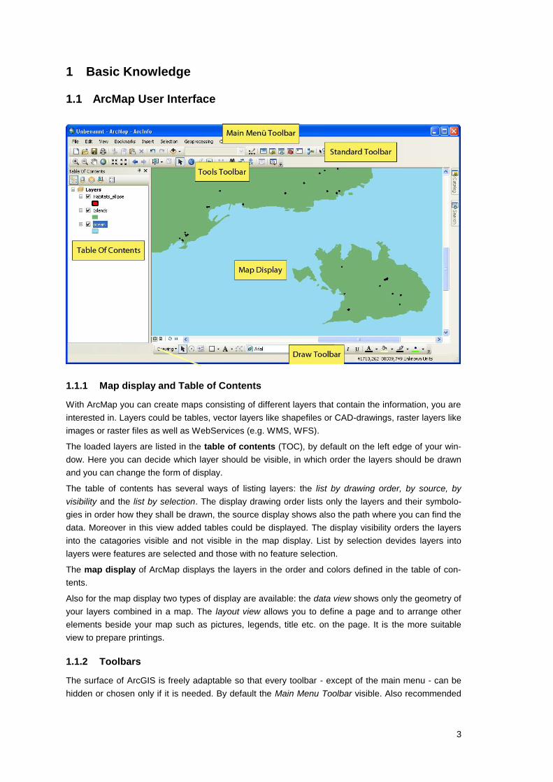
1.1 ArcMap User Interface
1.1.1 Map display and Table of Contents
With ArcMap you can create maps consisting of different layers that contain the information, you are
interested in. Layers could be tables, vector layers like shapefiles or CAD-drawings, raster layers like
images or raster files as well as WebServices (e.g. WMS, WFS).
The loaded layers are listed in the table of contents (TOC), by default on the left edge of your win-
dow. Here you can decide which layer should be visible, in which order the layers should be drawn
and you can change the form of display.
The table of contents has several ways of listing layers: the list by drawing order, by source, by
visibility and the list by selection. The display drawing order lists only the layers and their symbolo-
gies in order how they shall be drawn, the source display shows also the path where you can find the
data. Moreover in this view added tables could be displayed. The display visibility orders the layers
into the catagories visible and not visible in the map display. List by selection devides layers into
layers were features are selected and those with no feature selection.
The map display of ArcMap displays the layers in the order and colors defined in the table of con-
tents.
Also for the map display two types of display are available: the data view shows only the geometry of
your layers combined in a map. The layout view allows you to define a page and to arrange other
elements beside your map such as pictures, legends, title etc. on the page. It is the more suitable
view to prepare printings.
1.1.2 Toolbars
The surface of ArcGIS is freely adaptable so that every toolbar - except of the main menu - can be
hidden or chosen only if it is needed. By default the Main Menu Toolbar visible. Also recommended
4
is to keep the Standard and the Tools toolbar visible. You can undock every toolbar and move it to a
preferred place of your window.
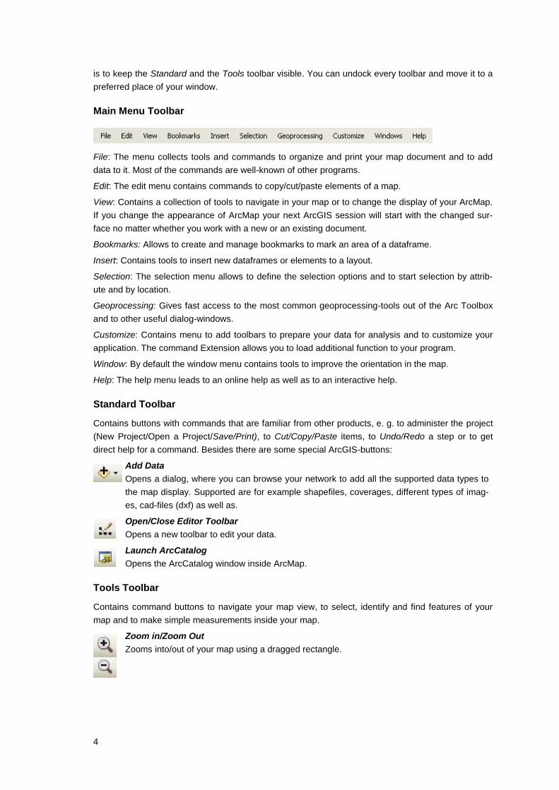
Main Menu Toolbar
File: The menu collects tools and commands to organize and print your map document and to add
data to it. Most of the commands are well-known of other programs.
Edit: The edit menu contains commands to copy/cut/paste elements of a map.
View: Contains a collection of tools to navigate in your map or to change the display of your ArcMap.
If you change the appearance of ArcMap your next ArcGIS session will start with the changed sur-
face no matter whether you work with a new or an existing document.
Bookmarks: Allows to create and manage bookmarks to mark an area of a dataframe.
Insert: Contains tools to insert new dataframes or elements to a layout.
Selection: The selection menu allows to define the selection options and to start selection by attrib-
ute and by location.
Geoprocessing: Gives fast access to the most common geoprocessing-tools out of the Arc Toolbox
and to other useful dialog-windows.
Customize: Contains menu to add toolbars to prepare your data for analysis and to customize your
application. The command Extension allows you to load additional function to your program.
Window: By default the window menu contains tools to improve the orientation in the map.
Help: The help menu leads to an online help as well as to an interactive help.
Standard Toolbar
Contains buttons with commands that are familiar from other products, e. g. to administer the project
(New Project/Open a Project/Save/Print), to Cut/Copy/Paste items, to Undo/Redo a step or to get
direct help for a command. Besides there are some special ArcGIS-buttons:
Add Data
Opens a dialog, where you can browse your network to add all the supported data types to
the map display. Supported are for example shapefiles, coverages, different types of imag-
es, cad-files (dxf) as well as.
Open/Close Editor Toolbar
Opens a new toolbar to edit your data.
Launch ArcCatalog
Opens the ArcCatalog window inside ArcMap.
Tools Toolbar
Contains command buttons to navigate your map view, to select, identify and find features of your
map and to make simple measurements inside your map.
Zoom in/Zoom Out
Zooms into/out of your map using a dragged rectangle.

5
Zoom in/Zoom Out
Zooms into/out of your map using system-given scales keeping the view center.
Pan
Changes the considered map view by dragging the map to the wanted direction.
Full extent
Zooms to the full extent of your map.
Previous/Next extent
Zooms to the previous/next extent.
Select features
Selects the elements of the predefined selectable layers.
Select elements
Select graphics in the map (e. g. text).
Identify
Tool to query the attributes of a chosen feature. The information will be shown in a popup
window.
Find
Opens a window to type in a word, that will be searched in all attribute tables of the loaded
layers.
Measure
Tool to measure distances by clicking the start- and the endpoint. The result is shown at the
status bar at the bottom of ArcGIS.
Hyperlink
Opens another document such as image or text files or starts a macro that is linked with the
features of a layer.

6
1.2 Exercise Explore ArcMap
Task
For the islands Gozo and Comino a map exists, that shows the agricultural use, the roads and the
cities of both islands. Check the map to get familiar with the data.
Data
All the used data comes from the Malta Environmental and Planning Authority (MEPA) or the survey-
office of Malta.
Used functions
Navigating a map
Make layers visible
Use tools for orientation in your map
How to do this
1. Preparing the data
Windows Right-click the Start button and point to Explorer to launch the
Windows Explorer. Copy the folder Exercise with the origin
data to your personal folder.
2. Navigating a map
Windows Double-click the ArcMap icon on your desktop or click the
Start button and point to Programs - ArcGIS - ArcMap to
launch ArcMap.
ArcMap dialog In the text box double-click Browse for more …, browse to
<personalfolder>/exercise/projects and choose
Expl_ArcMap.mxd. A map with the islands of Gozo and
Comino will open.
The layers are displayed in the order they appear in the table of contents (TOC). At present
a part of your layer Roads is hidden by the layer Development zones. Bring the Roads in
front of all other layers.
Table of contents (TOC)
Layer Roads
Select the layer to highlight it. Drag it to the top of the TOC.
While you are dragging a black bar shows you the present
position of your layer in the TOC.
Start to explore the map which contains the agricultural use, the roads and the cities of
Gozo.
Tools toolbar
Tool Zoom In
Drag a box around the westernmost end of the yellow major
road that crosses Gozo from west to east to zoom there. In
your Standard Toolbar point to the drop-down arrow next to
the scale and set the scale to 1:10.000.
Move the cursor to the blue polygon where the road ends. A
MapTip shows you that you are in Dwejra.

7
Tools toolbar
Tool Pan
Select the Pan tool and follow the road to the east. Every
time you pass a settlement with your cursor a MapTip shows
you the name of it. Finish to pan the map, when the MapTip
shows that you have reached the capital Rabat (Victoria).
3. Use orientation tools
To get an impression where the capital is situated and which extent you just view you can
use the Overview window of ArcMap.
Main menu Windows,
command Overview
The overview window opens normally with the bottommost
layer of the TOC as reference layer. In our case it is an or-
thophoto of Comino that is not suitable for an overview. To
change the reference layer right-click on the title bar of the
window and select properties.
Overview properties Click the drop-down arrow and choose Topographical Map
1:25.000 from the list. Press OK. The properties dialog dis-
appears and a small window shows the topographical map
with a red hatched rectangle marking the present extent.
Gozo & Comino Overview
window
Move the mouse cursor over the rectangle. A four-headed
arrow appears. Click inside the rectangle and drag it again to
the west coast. The extent of your map changes appropriate-
ly.
Move your cursor to a corner of the rectangle till it change to
a two-headed arrow. Click and drag to enlarge the rectangle.
The extent of your map changes appropriately.
Tools toolbar
Tool Previous extent
Undo your pan and zoom until you reach the capital again.
Close your overview window.
Tools toolbar
Tool Identify
Because we are interested in the area of the capital we query
its attributes. Click anywhere inside the blue area. The Identi-
fy window appears and shows depending on your choice
either the attributes of the Topographical map or of the roads
- the <Top-most layer> that is preselected by default. Change
the identified layer from the drop-down menu to Development
zones.
Click again inside the blue area. It blinks once green and the
Identify window lists the attributes which it took from the
table. The area in hectares should be 1’374‘695 m. Close the
Identify window.
4. Create spatial bookmarks
For a later quick access to the capital we want to create a spatial bookmark there. To begin
we want to zoom automatically to the area of the capital. Therefore we select the capital.
TOC
list by selection,
layers
Enable the posibility to be selected for the layers Roads and
Agricultural Use by clicking the colored boxes beside the
layernames. If you now use the Select features tool only
features from the layer Development zones are selectable.
8
Tools toolbar
Tool Select features
Click once inside the blue area of Rabat. Its outline will be
highlighted in blue color.
TOC
Layer Development zones
Right-click on the layer name and Zoom To Selected Fea-
tures. The view extent zooms automatically to the extent of
the capital.
Menu Bookmarks,
command Create
Select Create... The Spatial Bookmark window appears and
asks for a name. Insert Capital Rabat and press OK.
Menu Selection,
command Clear Selected
Features
The Selection of the capital will be removed.
Tools toolbar,
tool Full extent
Zoom to the full extent of the map.
Another spatial bookmark was already created for the island Comino. Use this bookmark to
zoom to the small eastern island.
Menu Bookmarks,
command Comino
Select Comino. Your map extent is set to the island.
Tools toolbar
Tool Measure
Use the measure tool, to give a statement to this island.
What’s the approximated extent of Comino?
North-South: ______ m; East-West: ______ m
TOC
List by visibility
Layer 3885o.jpg
In your table of content klick the box next to 3885o.jpg to turn
the layer on. A quadratic orthophoto will be drawn on the
western end of the island.
TOC
Layer 3885o.jpg
Zoom to the whole extent of your orthophoto by right-click on
the layer name and point to Zoom To Layer.
TOC
List by visibility
layers
Turn off the Agricultural Use, Topographical map and Gozo &
Comino by clicking their boxes to see the orthophoto without
impairment.
Use the navigating tools from your Tools toolbar to explore
the orthophoto.
TOC
Layer 3985o.jpg
Feel free to explore the other orthophoto.
Tools toolbar,
tool Full extent
Zoom back to the full extent of the map.
Main menu File,
Command Exit
Exit the map. Click Yes if you are prompted to save.

9
1.3 ArcCatalog User Interface
By default the ArcCatalog User Interface consists of the following components. If you change the
appearance of your Interface the next session will start with the changed surface.
1.3.1 Catalog display and catalog tree
Catalog tree
The catalog tree lists your data in a tree-like way similar the Windows Explorer, with plus signs and
minus signs to expand or hide the content of a drive or folder. Different from your Windows Explorer
the viewed data files are only the spatial data files of the dataset.
From the symbol next to the file name you can directly get the feature type of a vector data file:
Polygon
Line
Point
While the main symbols are always the same, the color specifies the file type. The most common
types are
Grey: Geodatabase
Green: Shapefiles
Blue: CAD file
Yellow: Coverage
Other often used symbols are:
Image or raster data. Irrespective from the file type the icon is always the same for raster
data.
TIN Surface model
Catalog display
The catalog display has three tabs to show information about your data: Contents, Preview, Descrip-
tion.
10
The Contents Panel allows to explore the content of a folder. You can choose different kinds of
displaying the data: large icons, simple list, list with details or thumbnails. The different view modes
can be chosen from the Standard toolbar.
Using the Preview Panel the geometry or the attribute table of a dataset can be viewed. (Enabling
the ArcGIS 3D Analyst extension allows the 3D View tools to navigate around your data in 3D). The
preview allows you to check your data quickly to decide which one is the best to add to ArcMap.
Preview is only possible when a dataset with geographical content is chosen. While the Geography
preview mode is active the Geography toolbar is enabled to navigate through the dataset.
The Description Panel shows information about the selected dataset that is stored in an xml-file
named like the dataset. If still no metadata exist for the selected dataset the Metadata preview cre-
ates a new xml-file at the same path location. With the Description toolbar you can print, edit or
import metadata.
1.3.2 Toolbars
As in ArcMap the surface of ArcCatalog is free adaptable. Every toolbar can be hidden or chosen
only if it is needed. By default the Main Menu Toolbar is visible. Advisable is to keep the Standard
and the Geography toolbar visible. You can undock every toolbar and move it to a preferred location
of your window by click on the gray bar and drag it to the target location. A frame shows you the
current form and position if you would drop the toolbar.
Main menu toolbar
File: Beside commands which can also be found in the Standard toolbar (such as Delete or Con-
nect/Disconnect) the command New allows to create a new folder or dataset.
Edit: Contains commands which are to be found in the Standard toolbar (such as Copy/Paste or
Search).
View: Controls the surface of ArcCatalog. Toolbars can be displayed or hidden as well as the Status
Bar and the Catalog tree.
Go: Contains the Up One Level command of the Standard toolbar.
Geoprocessing: Gives fast access to the most common geoprocessing-tools out of the Arc Toolbox
and to other useful dialog-windows.
Customize: Contains menu to add toolbars to prepare your data for analysis and to customize your
application. The command Extension allows you to load additional functions to your program.
Windows: Contains additional dialog-windows.
Help: Contains well-known and extensive help tools and information about the currently used ver-
sion.
Standard toolbar
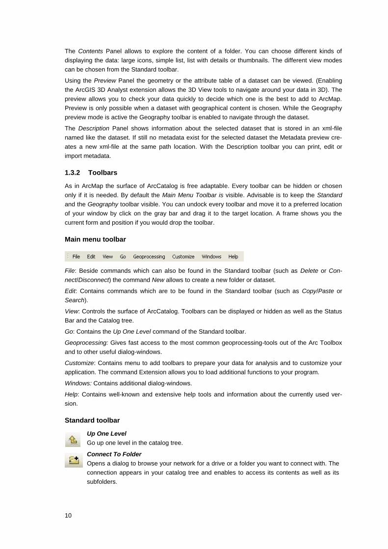
Up One Level
Go up one level in the catalog tree.
Connect To Folder
Opens a dialog to browse your network for a drive or a folder you want to connect with. The
connection appears in your catalog tree and enables to access its contents as well as its
subfolders.

11
Disconnect from folder
Disconnect and delete the currently selected folder connection from your catalog tree.
Copy/Paste/Delete Dataset
All three commands handle all the files that are connected with the selected item. E. g. for
shapefiles the action will be taken at least for the shp-, shx- and the dbf-file.
Copy copies the selected items into the clipboard. Paste adds the content of the clipboard
at the current location. Delete removes the selected items. For the last action is no undo
available so be careful to use this command.
View modes
View modes are only enabled if the Contents tab is chosen.
Large icons shows the content of the current location as icons.
List lists the content of the current location only by name.
Details lists the content of the current location with details. The viewable details can be set
in the options.
Thumbnails shows the content of the current location as small thumbnail images. A thumb-
nail is only shown when it was created before. ArcMap document files are automatically
shown as a thumbnail, other datasets such as shapefiles or coverage can get a thumbnail
by using the Create Thumbnail tool in the Geography toolbar.
Search tool
Allows searching for a dataset using defined search criteria like name, content or date.
Launch ArcMap
Launches the ArcMap application.
Launch Toolbox
Launches the ArcToolbox application.
What’s this?
Click this tool and point to any command or tool you are interested in to get a short descrip-
tion about it.
Geography toolbar
Zoom in/Zoom Out
Zooms into/out of your map using a dragged rectangle.
Pan
Changes the considered map view by dragging the map to the wanted direction.
Full extent
Zooms to the full extent of the chosen dataset.
Identify
Tool to query the attributes of a chosen feature. The information will be shown in a popup
window.
Create thumbnail
Is only active if Preview tab and Geography mode are chosen. Allows creating a thumbnail
to view the content in the thumbnail view.

12
Location toolbar
The location toolbar shows the path of the currently selected item.
For quick access to an item with known location you can type in the path and press enter.
1.4 Exercise Explore ArcCatalog
Task
Examine the data of Exercise 1.3.
Used functions
Connect to folder
Preview information about data
Use orientation tools
How to do this
1. Create connections
Windows Click the Start button and point to Programs - ArcGIS -
ArcCatalog to launch ArcCatalog.
By default only the local drives are shown in the catalog tree. Because we don’t want to
browse every time all the subfolders of our drive we want to create a connection to our
exercise folder.
Standard toolbar
Tool Connect To Folder
Click the button to open the Connect to Folder dialog.
Browse to your exercise folder. Use the plus signs to view
the content of a drive or folder.
Select the subfolder Exercise in your personal folder and
click OK. The connection <personalfolder>\exercise ap-
pears in the catalog tree.
2. Explore the Malta data
Catalog tree Click the plus sign next to your exercise folder to see the
content of it.
There should be five folders: images which stores raster data such as orthophotos or
topographical maps, projects that contains map documents and map templates, shape with
the vector data, tables with additional tables and import with original data in different data
formats.
Catalog tree Browse to the folder exercise/images/topmap and view its
content. Make sure that the Contents Panel is selected in
the catalog display.
Standard toolbar
Tool List
Choose the list view. A topographical map named mal-
ta_25.png should appear in the catalog display.
If you can’t see the file extension png change the settings to get it.
Main menu Customize,
command Arc Catalog
Options…
Open the ArcCatalog Options … dialog and choose the
General tab. Uncheck the box next to <Hide file extensions>
if necessary. Click OK to close the dialog.

13
Catalog tree Browse to the folder exercise/shape to preview the vector
data.
Standard toolbar
Tool Details
Choose the view with a list of detailed information about
your data.
You can set the kind of details you want to view.
Main menu Customize,
command Arc Catalog
Options…
Again open the ArcCatalog Options … dialog and choose
the Contents tab. Check the boxes next to <Name>, <Type>
and <Size>. Uncheck all the other boxes. Click OK to close
the dialog.
Your detail view shows now the selected details.
Standard toolbar
Tool Thumbnails
Choose the thumbnail view. At the moment only symbols but
no thumbnail should be visible.
Catalog tree Select the shapefile AGRI.shp. Choose the Preview Panel of
your catalog display. By default its geography is shown.
Geography toolbar
Tool Create Thumbnail
Click the tool to create a thumbnail.
Catalog tree Go back to the folder shape and make the Content Panel
active.
Standard toolbar
Tool Thumbnails
If you now choose the thumbnails view a small image of the
shapefile AGRI.shp should be visible.
! Repeat creating thumbnails for the other shapefiles in the folder.
Catalog tree Select the shapefile AGRI.shp again. Choose the Preview
Panel of your catalog display to view its geography.
Standard toolbar
Tool Zoom In
Drag a box anywhere at the island to zoom in.
Tools toolbar
Tool Identify
Click on any feature you are interested in. It blinks once
green and an Identify Results windows pops up and shows
the attributes of the feature. Scroll down to the field SUM-
MARY_DE to get the land use type.
Close the Identify Results window.
Standard toolbar,
tool Full extent
Zoom back to the full extent of the map.
There are a number of preview options. You can view the geography of your datasets,
the attribute tables, or the item descriptions
Catalog display From the drop-down menu next to <Preview:> on the bottom
of the catalog display choose Table.

14
Catalog display Now the attribute table will be displayed. On the bottom the
number of records (rows) is visible.
How many records are contained in the table? _______
For later orientation metadata should exist for every dataset. If you get data from an extern
association without metadata you can create your own metadata set. When you create
your own data however you should also create metadata.
Your Malta data contain no metadata yet. Only for the topographical map metadata was
created by the MLA staff.
Catalog tree Browse to the folder …/exercise/images/topmap and click
malta_25.png. Choose the Preview tab to get an impression
of the map. A dialog asks you whether ArcGIS should build
pyramids or not. Choose Build pyramids.
Geography toolbar
Tool Create Thumbnails
When the image is ready build, create a thumbnail.
Catalog display Choose the Description Panel. If the previous action was
successful, you should see a small image of the map. Ex-
plore the metadata. To see the content of a green heading
click on it.
Main menu File,
command Exit
If you do not want to continue with the next exercise finish
the program.

15
1.5 Layouts
ArcMap provides two ways to view a map: data view and layout view. Although you could print a map
directly from the data view ArcGIS provides a layout view to work with the map layout elements such
as titles, north arrows or scale bars.
If you want to display more than one data frame (e. g. a detailed and an overview map) you can
display its spatial relations by showing extent rectangles.
For further use you can save map templates from already created maps to produce maps that con-
form to a standard. Moreover they save time by letting you do the layout work for all of the maps in
the series at once.
1.6 Exercise Creating maps
Task
For a short presentation of the island of Gozo you want to create the overview map you explored in
the first exercise using your own colors and symbols.
Data
The vector data was created and made available by the Malta Environment and Planning Authority
(MEPA). The topographical map was scanned from an analogue map 1:25.000 and georeferenced
by the MLA staff. It is available as a png-file.
Used functions
Symbolize the data
MapTips, labeling
Create a layer file from your symbolized data
Create bookmarks
Extent rectangles
Use templates for layouts
How to do this
1. Create a new map
Start the program, create a new map document and add some data.
Windows Double-click the ArcMap icon on your desktop or click the
Start button and point to Programs - ArcGIS - ArcMap to
launch ArcMap.
ArcMap dialog
blank map
Create a new empty document.
Standard toolbar
Tool Add Data
Browse to <personalfolder>/exercise/shape, select the
feature datasets agri.shp, dev_zone.shp and str.shp by click
on it and point to Add to add the dataset to your map. To
choose more than one dataset at the same time press the
CTRL key.
Confirm the warning that one or more layer miss’s spatial
information. The layers will be displayed in the map.

16
At time the map has no scale. Set the properties of the display to change this.
Main menu View,
Data Frame Properties…
Open the Data Frame Properties and click the General tab.
Change the name of your data frame in Gozo & Comino and
set the map units and the display units to meters. Click OK
to apply your changes.
The layers are displayed in the order they appear in the table of contents (TOC). Bring it in
the following order (from top) if necessary: str.shp, dev_zone.shp, agri.shp.
TOC
List By Drawing Order
To change the order of the layers click the layer you want to
move and drag it to the target position.
Standard toolbar
Tool Save
Save your map document as exercise1-6.mxd to your <per-
sonalfolder>/exercise/projects.
2. Symbolize your data
At present all the features in each layer are displayed in the same way: same (randomly
chosen) color, same outline, same hatching and so on. We want to change the symbology
based on the attribute table.
TOC
Layer str.shp
Double-click the layer str.shp to open the Layer Properties
dialog or open it by right-click on the layer and point to
Properties…. Choose the Symbology tab.
In the <Show> box on the left side by default Single symbol
is chosen for every feature. Change the method of symboliz-
ing to Categories and Unique values. From the drop-down
menu next to <Value Field> choose the field FEATCO,
which contains different categories of streets. Click Add All
Values.
In the former empty list five different categories each with another symbol appear. The
Value column shows the coded categories of the streets on Gozo. The roads which code
starts with a W3 are major roads, these with a W8 are secondary roads and those with
W04 are gravel roads. Rename the road codes in the Label column using its meaning.
Layer Properties str.shp Click once the W04 in the <Label> column and replace the
text with Gravel roads.
Select now the roads with the value W35 and W36. To
select more than one value use the CTRL key. Right-click
and point to Group Values. Both values appear in one line.
Rename the label to Major roads.
Repeat the step equivalent for the remaining values and
rename it to Secondary roads.
Rename the Heading FEATCO in Type.
Now the road symbology should be displayed in a different way depending on their im-
portance.
17
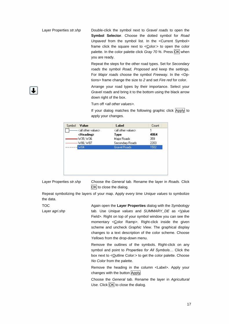
Layer Properties str.shp Double-click the symbol next to Gravel roads to open the
Symbol Selector. Choose the dotted symbol for Road
Unpaved from the symbol list. In the <Current Symbol>
frame click the square next to <Color:> to open the color
palette. In the color palette click Gray 70 %. Press OK when
you are ready.
Repeat the steps for the other road types. Set for Secondary
roads the symbol Road, Proposed and keep the settings.
For Major roads choose the symbol Freeway. In the <Op-
tions> frame change the size to 2 and set Fire red for color.
Arrange your road types by their importance. Select your
Gravel roads and bring it to the bottom using the black arrow
down right of the box.
Turn off <all other values>.
If your dialog matches the following graphic click Apply to
apply your changes.
Layer Properties str.shp Choose the General tab. Rename the layer in Roads. Click
OK to close the dialog.
Repeat symbolizing the layers of your map. Apply every time Unique values to symbolize
the data.
TOC
Layer agri.shp
Again open the Layer Properties dialog with the Symbology
tab. Use Unique values and SUMMARY_DE as <Value
Field>. Right on top of your symbol window you can see the
momentary <Color Ramp>. Right-click inside the given
scheme and uncheck Graphic View. The graphical display
changes to a text description of the color scheme. Choose
Yellows from the drop-down menu.
Remove the outlines of the symbols. Right-click on any
symbol and point to Properties for All Symbols… Click the
box next to <Outline Color:> to get the color palette. Choose
No Color from the palette.
Remove the heading in the column <Label>. Apply your
changes with the button Apply.
Choose the General tab. Rename the layer in Agricultural
Use. Click OK to close the dialog.
18
! Symbolize the layer dev_zone.shp yourself. Apply again unique values. Use the field
FEATURE for value field. Change the symbol of Industrial Area to Blue Gray Dust, for
Urban Area to Tuscan Red. Remove the heading and rename the layer to Settlements.
3. Label your map with MapTips and labels
Because the yellow colors of the agricultural used areas are often similar you want to
support the identification with MapTips.
TOC
Layer Agricultural Use
Double-click the layer name to open its properties. Choose
the Display tab. Pick from the drop-down list next to <Dis-
play Expressions:> the field SUMMARY_DE. Check the box
<Show Map Tips using display expressions>. Click OK.
If the command is not selectable close the dialog clicking OK.
Standard toolbar
Tool Editor Toolbar
Open the Editor toolbar if necessary.
Editor toolbar
Menu Editor
In the Editor menu select Start Editing to start an
edit session. Double-click any Value Field of the
layer Agricultural Use. Close the window Template
Properties.
Stop the edit session using Stop Editing in the
Editor menu.
Standard toolbar
Tool Editor Toolbar
Close the Editor toolbar.
TOC
Layer Agricultural Use
Again open the layer properties of Agricultural Use
by double-click on the layer name. Choose the
Display tab. Check <Show Map Tips using display
expressions> should now be possible. Click OK.
Map display Move your cursor over your map. The respective field type
will be displayed as MapTip.
Moreover we want to display the cities names at all times.
TOC
Layer Settlements
Double-click the layer name to open its properties. Choose
the Labels tab.
Tick <Label Features in this layer>. For label <Method>
make sure that Label all the features the same way is cho-
sen. In the <Text String> frame choose NAME from the
drop-down list next to <Label Field:>.
Click the Symbol…. tool in the <Text Symbol> frame. The
Symbol Selector will be opened. Choose Country 2 as font
type. In the <Current Symbol> frame set the color to Gray
70 %. Keep the other settings and click OK to close the
Symbol Selector.
In the <Other Options> frame click the Placement Proper-
ties. In the opened Placement Properties dialog check
<Remove duplicate labels>. Click OK to close the Place-
ment Properties window.
Press OK to close the Layer Properties dialog. The names
of the settlement appear in the chosen way.
19
TOC
Layer Settlements
Double-click the layer name to open the Layer Properties
dialog. Choose the Label tab and klick in the <Other Op-
tions:> frame Scale Range. Make sure that Use the same
scale as the feature layer is chosen. Click OK to close the
dialog.
Standard toolbar
Map scale
Type a scale of 25000 in the text box. Press the Enter key to
confirm the entered scale.
TOC
Dataframe
Right-click on the Dataframe and open Reference Scale Set
Reference Scale.
Standard toolbar,
tool Full extent
Zoom back to the full extent of the map. Your labels are
displayed scaled now based on the defined Reference Scale
of 25.000.
4. Create a bookmark
Tools toolbar
Tool Zoom in
Drag a rectangle around Comino to zoom there. Chose per
Drag & Drop a scale of 25000 in the text box of the map
scale.
Tools toolbar
Tool Pan
Use the pan tool to centralize Comino inside the display.
Menu View
Command Bookmarks
Create
Type in the appearing Spatial Bookmark dialog next to
<Bookmark Name:> Comino and press OK.
Standard toolbar,
tool Full extent
Again zoom back to the full extent of the map.
Tool Save Save your map.
5. Create layer files
We invested some work and time to change the appearance of our layers. To avoid the
same work every time we use a layer in a new map document we want to store the settings
of our layers.
TOC,
Layer Roads
Right-click on the layer name and point to Save as Layer
File…. The Save Layer dialog prompted for the path.
Choose <personalfolder>/exercise/shape and save it using
the suggested name.
Windows Open ArcCatalog.
ArcCatalog!
Catalog tree Browse to your <personalfolder>/exercise/shape.
Catalog display Choose the Contents tab.
Standard toolbar,
Tool Large Icons
Your new created layer file appears as a yellow square that
stands on one corner.
20
Catalog display Select the Icon for your file Roads.lyr and choose the Pre-
view tab. The layer appears in the same way you created in
your map document.
Geography toolbar
Tool Create Thumbnails
Click the tool to create a thumbnail.
Catalog display Go back to the Contents tab. You should see a little thumb-
nail of your Roads layer file.
! Go back to ArcMap and create layer files from the other data. Create thumbnails in
ArcCatalog for it. If you can’t see your new files in ArcCatalog select the folder where it is
saved and press F5 to refresh the content of the folder.
6. Overlay the topographical map
To complete our map we want to add the topographical map 1:25.000.
ArcCatalog!
ArcCatalog Arrange and resize your ArcCatalog window that you can
see ArcMap in the background
Catalog tree Browse to your <personalfolder>/exercise/images/topmap.
Standard toolbar,
Tool Thumbnails
Display the thumbnails of your data. Make sure that the
Contents tab is chosen in the catalog display.
Standard toolbar,
Tool Details
Choose the detailed display. Select the malta_25.png by
click on it. If it is selected it is blue highlighted. Drag it to
ArcMap.
Go back to ArcMap.
ArcMap!
TOC
List By Drawing Order
Drag malta_25.png to the top of your table of content if
necessary.
TOC
Layer malta_25.png
Double-click the layer name to open the Layer Properties
dialog. Choose the Display tab. Type 50 into the text box
next to <Transparency>. Click Apply or OK to see the
changes.
7. Create a new Data Frame
Main Menu Insert,
Command Data Frame
Create a new Data Frame. It will be inserted at the bottom of
your table of contents as New Data Frame.
TOC
New Data Frame
Double-click on the name of your new data frame to get the
Data Frame Properties dialog. Choose the General tab if
necessary. Rename the data frame next to <Name:> into
Overview and set the map and display units to Meters.
The new data frame is still empty. For an overview we insert the topographical map
1:25.000.
TOC
Data frame Gozo & Com.
Layer Malta_25.png
Right-click the layer name and point to Copy to bring Mal-
ta_25.png into the clipboard.

21
TOC
Data frame Overview
Right-click the data frame name and point to Paste Layer to
insert Malta_25.png from the clipboard.
TOC
Data frame Overview.
Layer Malta_25.png
Double-click the layer name to open its properties. Choose
the Display tab and set the transparency to 0 %. Press OK.
TOC
Data frame Gozo & Com.
Right-click the data frame name and point to Activate to
make the first data frame active.
Menu Bookmarks
Command Comino
Zoom to the extent of Comino using the bookmark.
8. Create a layout using a template
Map display bottom
Tool Layout View
Change your map display from the data view to the layout
view. A page with both created maps appears. Moreover the
Layout toolbar pops up.
Menu File
Command Page and Print
Setup…
In the Page and Print Setup dialog in the <Map Page Size>
frame turn off the checkbox next to <Use Printer Paper
Settings> if necessary. Choose from the <Standard Sizes:>
drop-down list A2, and choose Landscape for <Orienta-
tion:>. Press OK.
Layout toolbar
Tool Change Layout
Choose the My Template tab from the Select Template
dialog.
Select Template dialog Click the Open template button on the bottom of your dialog
to browse to <personalfolder>/exercise/projects, select the
Template_3_1.mxd and click Open.
The next window gives a preview to the order of the data-
frames. Move the dataframe Overview to the top by select-
ing it and pushing the button <Move Up>.Click Finish to
close the dialog and to apply the template.
The layout changes according to the template with arranged data frames.
Standard toolbar
Scale
Click once in the frame with the island Comino to get it
marked by a dotted line. Pick from the drop-down list in the
Standard toolbar the scale 1:10.000.
To see the location of Comino in our overview map we want to create an extent rectangle.

22
Map display Click once into the right frame with the overview map to get
this frame marked. Right-click inside the map and point to
Properties. In the Data Frame Properties choose the Extent
Indicators tab. In the textbox next to <Other data frames:>
select Gozo & Comino and click the single arrow to the right.
The data frame will appear in the box next to <Show extent
indicators for these data frames>. Click the Frame button.
In the Extent Indicator Frame Properties dialog pick the
borderline 4,0 Point from the drop-down list in the <Border>
frame. Click the rectangle next to <Color:> to get the color
palette and choose Ginger Pink. Press OK to close the
Frame Properties and again to close the Data Frame
Properties.
In your overview map should appear a rectangle that shows
the extent of the map beside it.
Map display Click the title of the layout to get it edged dotted. Right-click
on it and select Properties. In the appearing Properties
dialog choose the Text tab if necessary. Click inside the text
box and replace the existing text with Island Comino. Click
OK.
! Enter your name and the present date in the boxes below the map frames.
Finally we want to add legend, scale bar and north arrow to our layout.
Layout toolbar
Tool Zoom Whole Page
Zoom to the extent of your whole layout page.
Menu Insert
Legend...
Make sure that the frame with Comino is selected before
choosing the command.
Legend Wizard In the appearing Legend Wizard you can specify which item
you want to display. By default all the items are selected.
Remove Malta_25.png from the list next to <Legend Items>
by selecting it and press the button with the single arrow to
the left < . Click Next.
The next window treats the legend title. Delete Legend from
the textbox. Click Next.
Confirm all the following settings clicking Next respectively
Finish to close the dialog and create the legend.
At the moment there is no layer name written. Furthermore we decide because of the
amount of patches in the legend to display it using two columns.
23
Tools toolbar
Tool Select Elements
Double-click the legend. In the Legend Properties dialog
choose the Items tab. To change the style of all legend
items select all the items in the box beneath <Legend
Items:> using the Shift key. Afterwards click the Style…
button to open the Legend Item Selector. Choose Horizon-
tal Single Symbol Layer Name and Label from the list. Click
OK.
Select from the list beneath <Legend Items:> the Agricultur-
al Use and check the check box next to <Place in new
column>. Click OK.
Tools toolbar
Tool Select Elements
Move the created legend to the empty space in the upper
right corner of your layout.
! Change the spacings between the columns and objects of your legend. Use for this pur-
pose the Legend tab of the Legend Properties dialog.
Menu Insert
North Arrow...
Pick one of the north arrows from the appearing North
Arrow Selector. Press OK. The arrow will be inserted in the
middle of your page.
Tools toolbar
Tool Select Elements
Drag it to the frame down right of your layout.
Menu Insert
Scale Bar...
In the Scale Bar Selector select the Hollow Scale Bar 1 and
click OK.
Tools toolbar
Tool Select Elements
Drag it to the empty space in the left down corner of the
Comino data frame. To change its properties double-click
the scale bar.
Hollow Scale Bar Properties Choose the Scale and Units tab if necessary. In the
<Scale> frame select Adjust width from the drop-down menu
next to <When resizing…>. Set for <Division value:> 500 m.
Type next to <Number of divisions:> 3 and next to <Number
of subdivisions:> 2. In the <Units> frame select Meters
beneath <Division Units> and after labels beneath <Label
Position> and replace Meters next to <Label:> with m. Press
OK.
! Enter a free eligible text in the middle field on the bottom of your layout. Choose the com-
mand Text from the main menu Insert.
Layout toolbar
Tool Zoom Whole Page
Zoom to the extent of your whole layout page if necessary. It
should match roughly the following graphic.
Standard toolbar
Tool Save
Save your map document.

24
25
1.7 Exercise Create and modify data
Task
Someone has started to digitize the contour lines based upon the topographical map. Obviously the
digitizer couldn’t come to the end so the contour lines are still unfinished. You want to continue
digitizing this layer.
Moreover there is a shapefile with the borders of all islands but with apparent mistakes and missing
data. Your task is to correct the data.
Another task is to create a tourism guide for Gozo and Comino. Therefore you will start with a new
shapefile that contains caves on both islands.
Data
Available is the georeferenced topographic map of Gozo in the scale 1:25.000 as png-format as well
as a shapefile that contains beside others the caves and a dxf-file with the contour lines.
Used functions
Digitize features in an existing shapefile
Deal with the attribute table
Change the display of your data
Modify features
Create shapefiles
Create metadata
How to do this
1. Prepare your map
Windows Double-click the ArcMap icon on your desktop or click the
Start button and point to Programs - ArcGIS - ArcMap to
launch ArcMap.
ArcMap dialog
blank map
Create a new empty document.
Main menu View,
Data frame properties
Open the data frame properties and click the General tab.
Change the name of your data frame in Changing Geometry
and set the map units and the display units to meters. Click
OK to apply your changes.
Tool Add Data Browse to <personalfolder>/exercise/images/topmap/, select
the image malta_25.png and point to Add. Repeat the step
for the layer Habitats_ellipse.shp from your folder <personal-
folder>/exercise/shapes.
Furthermore add the linear elements from the dxf-file Eleva-
tion from <personalfolder>/exercise/import/. When you
browse to the given path two files are offered. Double-click
the one with the blue symbol to get its parts displayed. Now
choose Polyline and point to Add.
26
TOC
Layer Habitats_ellipse.shp
Double-click the layer name of Habitats_ellipse.shp to open
the Layer Properties dialog. Choose the
Symbology tab. From the list in the box beneath Show:
choose Categories and Unique values. In the box next to
<Value Field> the field FEATURE should already be cho-
sen. Point to Add Values and choose from the Add Values
dialog only the caves. Click OK to close the Add Value
dialog. Double-click the symbol next to CAVE to get the
Symbol Selector dialog. In the Options frame choose a red
fill color for it. Close all the dialogs by clicking OK.
Tool Save Save your map document as exercise1-7.mxd to your <per-
sonalfolder>/exercise/projects.
2. Digitize features
You want to start your tasks digitizing the contour lines. Because ArcGIS is unable to
modify dxf-files we have to transform the dxf-layer into another data format.
TOC
Layer ELEVATION.DXF
Polyline
Right-click to your layer name and point to Data and Export
Data… In the Export Data dialog click the folder symbol to
specify the path <personalfolder>/exercise/shapes/ and
name the new shapefile as contour. Keep all the other
settings and press OK. Click Yes if you are prompted
whether to add the new layer or not.
TOC
Layer ELEVATION.DXF
Polyline
The dxf layer is no longer necessary. Right-click on the layer
name and point to Remove to delete it from yout table of
content.
Every time you want to edit or modify features you have to start an edit session.
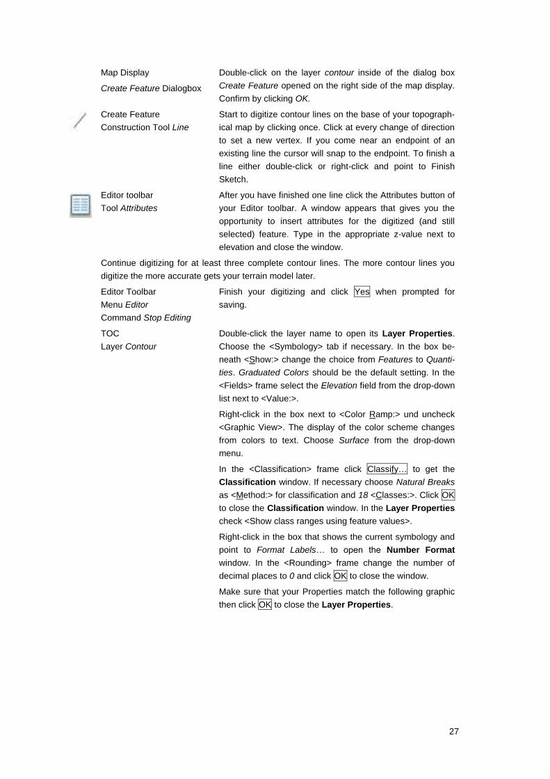
Tool Editor toolbar The fastest way to get the Editor Toolbar is the button in
your Standard Toolbar.
Editor toolbar
Menu Editor
Command Start Editing
Start the edit session in the Editor Toolbar. After have done
so, you can set in the dialog box the targed of your edit
session.
Editor toolbar Set contour for target if necessary.
Tools toolbar
Tool Zoom in
Drag a rectangle in an area where obviously contour lines
are missing.
Standard toolbar To improve the accuracy of our digitizing use a scale that is
bigger than this of the base map. In our case type 1:5.000 in
the scale box of your standard toolbar.
Our new digitized lines should join existing ones where it is possible so it is better to set
some snapping options.
Editor toolbar
Menu Editor
Command Snapping
Toolbar
Open the Snapping Toolbar and select End Snapping.
27
Map Display
Create Feature Dialogbox
Double-click on the layer contour inside of the dialog box
Create Feature opened on the right side of the map display.
Confirm by clicking OK.
Create Feature
Construction Tool Line
Start to digitize contour lines on the base of your topograph-
ical map by clicking once. Click at every change of direction
to set a new vertex. If you come near an endpoint of an
existing line the cursor will snap to the endpoint. To finish a
line either double-click or right-click and point to Finish
Sketch.
Editor toolbar
Tool Attributes
After you have finished one line click the Attributes button of
your Editor toolbar. A window appears that gives you the
opportunity to insert attributes for the digitized (and still
selected) feature. Type in the appropriate z-value next to
elevation and close the window.
Continue digitizing for at least three complete contour lines. The more contour lines you
digitize the more accurate gets your terrain model later.
Editor Toolbar
Menu Editor
Command Stop Editing
Finish your digitizing and click Yes when prompted for
saving.
TOC
Layer Contour
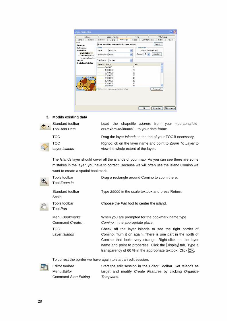
Double-click the layer name to open its Layer Properties.
Choose the <Symbology> tab if necessary. In the box be-
neath <Show:> change the choice from Features to Quanti-
ties. Graduated Colors should be the default setting. In the
<Fields> frame select the Elevation field from the drop-down
list next to <Value:>.
Right-click in the box next to <Color Ramp:> und uncheck
<Graphic View>. The display of the color scheme changes
from colors to text. Choose Surface from the drop-down
menu.
In the <Classification> frame click Classify… to get the
Classification window. If necessary choose Natural Breaks
as <Method:> for classification and 18 <Classes:>. Click OK
to close the Classification window. In the Layer Properties
check <Show class ranges using feature values>.
Right-click in the box that shows the current symbology and
point to Format Labels… to open the Number Format
window. In the <Rounding> frame change the number of
decimal places to 0 and click OK to close the window.
Make sure that your Properties match the following graphic
then click OK to close the Layer Properties.
28
3. Modify existing data
Standard toolbar
Tool Add Data
Load the shapefile islands from your <personalfold-
er>/exercise/shape/… to your data frame.
TOC Drag the layer Islands to the top of your TOC if necessary.
TOC
Layer Islands
Right-click on the layer name and point to Zoom To Layer to
view the whole extent of the layer.
The Islands layer should cover all the islands of your map. As you can see there are some
mistakes in the layer, you have to correct. Because we will often use the island Comino we
want to create a spatial bookmark.
Tools toolbar
Tool Zoom in
Drag a rectangle around Comino to zoom there.
Standard toolbar
Scale
Type 25000 in the scale textbox and press Return.
Tools toolbar
Tool Pan
Choose the Pan tool to center the island.
Menu Bookmarks
Command Create…
When you are prompted for the bookmark name type
Comino in the appropriate place.
TOC
Layer Islands
Check off the layer islands to see the right border of
Comino. Turn it on again. There is one part in the north of
Comino that looks very strange. Right-click on the layer
name and point to properties. Click the Display tab. Type a
transparency of 60 % in the appropriate textbox. Click OK.
To correct the border we have again to start an edit session.
Editor toolbar
Menu Editor
Command Start Editing
Start the edit session in the Editor Toolbar. Set Islands as
target and modify Create Features by clicking Organize
Templates.

29
Organize Feature Tem-
plates
Menü New Templates
Choose in the Organize Feature Templates dialog box the
layer Islands and click in the menü New Templates. Set the
check box beside the layer Islands and click <Finish>. Close
the Organize Feature Templates dialog box by clicking
<Close>. The features from the layer Island are now added
to the Create Feature window on the right side of the Map
display. Select Islands by clicking.
Tools toolbar
Tool Zoom in
Zoom nearer the part you want to correct. The new extend
of the border should match the 0 contour line.
Editor toolbar
Menu Editor
Command Snapping…
Snapping Toolbar
Open the Editor Toolbar and activate Vertex Snapping.
Editor toolbar
Tool Edit
Click once inside the polygon you want to modify, then right-
click and point to Edit Vertices. Its vertices are displayed.
For our aim we do not need all the vertices. Right-click on
one of the vertices and point to Delete Vertex. If there is only
one left move the cursor over it and drag it to the edge of the
contour line. Because of the set snapping option it should
snap to the vertex of the contour line.
Click anywhere outside to see your changes applied.
Tools toolbar
Tool Go back to the previ-
ous extent
The previous extent should be the one of whole Comino. If
not zoom to the full extent and drag again a rectangle
around Comino.
As you can see the small island Kemmunett (or Cominotto) isn’t still contained in the layer
Islands. You want to add this feature to the shapefile. Moreover you want to name the
islands in the attribute table.
The outline of the small island Cominotto corresponds to the contour line for 0. Therefore
we want to trace this line.
Tools toolbar
Tool Zoom in
Drag a rectangle around Cominotto.
Tools toolbar
Tool Select feature
To trace a feature you need to select it. Click once the
contour line for the elevation 0. It should become highlighted
in blue.
Map Display
Create Feature dialog box
Click the Construction Tool Polygon inside the Create Fea-
ture dialog box to activate the hidden tools in the Editor
toolbar. Choose the Trace tool. Click at any point on the
highlighted contour line and follow the outline around the
island. If you have reached the start point finish the feature
with a double-click.
Menu Selection,
Command Clear Selected
features
Remove the selection of the island.
Finally correct the island Gozo that momentary consist of two parts (one that covers almost
the whole island and one circular part). Both parts should become unionized.
30
TOC For a better view of the problem turn off all the layers except
of the Islands layer.
Tools toolbar
Tool Select feature
Drag a rectangle over both parts to get them selected and
highlighted.
Editor toolbar
Menu Editor
Command Merge.
Both parts are joined together.
The layer is now almost ready. For further information you want to add an attribute field
with the island name and the area of the island.
Editor Toolbar
Menu Editor
Command Stop Editing
To add an attribute field you have to finish the edit session.
Click Yes when asked for saving.
TOC
Layer Islands
Right-click on the layer name and point to Open Attribute
Table.
Attribute table of Islands
Menu Table Options
Command Add Field…
Open the Add Field dialog. Type in the text box next to
<Name:> English_Na and choose from the menu next to
<Type:> Text. Give the field a length of 20.
Repeat the step and add another text field called Mal-
tese_Na also with a field length of 20.
A third field shall be the field Area, field type Double with
unchanged other settings.
Start calculating the Area of the islands using an SQL statement.
Attribute table
Field Area
Right-click the Area field name and click Calculate Geome-
try…. A message reminds you, that outside an edit session
undo your calculating is not possible. Click Yes to continue.
In the appearing Calculate Geometry dialog choose out of
the drop-down list by <Property> Area if necessary.
Click OK. ArcGIS takes the area from the geographic fea-
tures and uses the units you have set in the data frame
properties, which means you get square meters!
Because square meters are to accurate to display the area you want to add a new field
that contains the area in hectares.
Attribute table of Islands
Menu Table Options
Command Add Field…
Add another field called Area_ha, field type Float, type for
<Precision> (field width) 8, and for <Scale> (digits right of
the comma) 2.

31
Attribute table
Field Area_ha
Right-click the Area_ha field, point to Field Calculator… and
confirm the warning.
To calculate hectares you can use the field Area divided by
10000.
To get the right expression double-click Area in the Fields
list. It appears in the text box beneath Area_ha= in angular
brackets. From the buttons right of the text box take the /
button by one click. Type finally 10000 in the text box so that
your expression matches the following:
[Area] /10000
Click OK and examine the results. Afterwards close the
attribute table.
What is now still missing are the names of the islands. To enter them you have to start the
edit mode again.
Editor Toolbar
Menu Editor
Command Start Editing
Inside the Start Editing dialog choose Islands as target and
confirm by clicking OK.
Tools toolbar
Tool Select feature
Start selecting the polygon of Gozo by click inside the poly-
gon.
Editor toolbar
Tool Attributes
Open the Attribute insert window and type Gozo next to both
English_Na and Maltese_Na.
Tools toolbar
Tool Select feature
Select the island of Comino.
Editor toolbar
Tool Attributes
Enter Comino next to English_Na and Kemmuna next to
Maltese_Na.
Repeat the step for Cominotto (Kemmunett). Southeast of Cominotto there are two small
islands with no names at it. Select them one after another and enter Unknown for their
names.
Still there are some little islands left. They are obviously too small to find them easily so
you can use the attribute table to search for them.
TOC
Layer Islands
Right-click on the layer name and point to Open Attribute
Table. Examine the records which have still no entry. Click
on the gray box left of one record with no entry to get it
highlighted. Minimize the attribute table so that you can see
the table of content.
Right-click on the layer Islands and point to Selection and
Zoom To Selected Features. Your map display switches to
the extent of the selected feature.
Tools toolbar
Tool Fixed Zoom Out
Zoom out until you can see whether there is a label on the
topographical map.
Editor toolbar
Tool Attributes
If there is an English and a Maltese label enter the names
next to English_Na and Maltese_Na. For those labels miss-
ing enter Unknown.

32
Restore the table and repeat the steps for every record with
missing entries. Close the table after finish all records.
TOC
Layer Islands
Double-click the rectangle symbol beneath the layer name to
get instantly the Symbol Selector dialog for it.
Symbol Selector Choose the Hollow symbol from the symbol list. In the right
frame click the button Edit Symbol….to open the Symbol
Property Editor. Choose the Outline… button to change its
appearance. In the Symbol Selector choose the symbol
category Dashed from the list and change in the <Current
Symbol> frame its <Width> to 2 and Mars Red for <Color>.
Click OK to close the Symbol Selector, again to close the
Symbol Property Editor and a third time to close the remain-
ing window.
TOC
Layer Islands
Save your display settings by right-click on the layer name
and point to Save As Layer File… Take the suggested name
Islands.lyr and save it to <personalfolder>/exercise/shape….
Because the Layer Islands has a transparency the 0 contour line shines through it. We
want to fade out the contour lines with the value 0.
TOC
Layer Contour
Double-click the line next to 0 to get the Symbol Selector.
In the <Current Symbol> frame choose No Color from the
drop-down list next to <Color:>. Close the dialog clicking
OK.
4. Create a new shapefile
To create a new layer you have to change to ArcCatalog.
Windows Point to Programs - ArcGIS - Arc Catalog to launch Arc
Catalog.
33
ArcCatalog!
ArcCatalog tree Browse to your personal project folder <personalfold-
er>/exercise/shape. Right-click the shape folder, point to
New and Shapefile…. A Create New Shapefile dialog pops
up.
Shapefiles can store only one type of geometry: either polygons or lines or points. Because
our shapefile should store the tourist attractions of the island of Gozo and Comino we
prefer to set the feature type to point.
Create New Shapefile
dialog
In the dialog type Attractions in the textbox next to <Name:>.
The drop-down list next to <Feature Type:> should show
Point by default. Click OK to finish. An empty shapefile
named Attractions is created in your shape folder.
Catalog display
Tab Preview
If you preview the geography of your new shapefile it is
completely empty. However, in the preview of the attribute
table should be at least three fields: FID, Shape and ID (but
no record).
Catalog tree Right-click on your layer Attractions.shp and point to Proper-
ties. In the Shapefile Properties click the <Fields> tab if
necessary.
In the column <Field Name> add a new field entering Type
in the next empty cell. In the column <Data Type> select
Text as data type. In the <Field Properties> frame in the
lower portion change the field length to 24. Click OK to get
the dialog closed and the new field added.
ArcCatalog window Reduce the size of your application window and arrange it to
see ArcMap beside it.
Drag your layer Attractions.shp to your map document in
ArcMap and change to ArcMap.
ArcMap!
5. Create point features
TOC
Layer Attractions
Drag your layer to the top of your table of content if neces-
sary.
You still should be in an edit session. If not start the edit session again.
Map Display
Create Feature dialog box
Click the Organize Templates button to open the Organize
Feature Templates. Choose the layer Attractions and open
the Create New Templates Wizard by clicking <New Tem-
plates> in the menü.
Check the box next to the layer Attractions if necessary and
continue with <Finish>. Close the Organize Feature Tem-
plates by clicking <Close>.
Select the layer Attractions in the Create Feature dialog box
at the right side of your map display.
The information about caves you take from the layer Habitats_ellipse. Although we already
changed the color of the caves to red they are not really good recognizable. Therefore we
want to zoom to the habitats which are caves.

34
Menu Selection
Command Select by Attrib-
utes…
Open the Select By Attributes dialog. From the drop-down
list next to <Layer:> choose Habitats_ellipse.
In the textbox in the lower portion of the dialog you make an SQL expression to query your
data. You can either type in the expression or you take the parts of the expression from
lists. The last one allows creating SQL statements without care about the syntax. To create
an expression, double-click the field you want to use, click an operator, then double-click
the value.
Select by Attributes dialog Create the expression "FEATURE" = 'CAVE' by double-click
the field “FEATURE” from the box beneath <Fields:>, simple
click the Equal to button and double-click ‘CAVE’ from
<Unique Values:>. Choose the Verify button to check your
expression and – if it was successful – Apply your selection
and Close the dialog.
TOC
Layer Habitats_ellipse
Right-click on the layer Habitats_ellipse and point to Selec-
tion and Zoom To Selected Features. Your map display
switches to the extent of the selected features which are
highlighted in blue.
TOC Turn off all layers except of Attractions, Islands and Habi-
tats_ellipse to have a better view onto the selected features.
Editor toolbar
Tool Sketch Properties
Use the Sketch tool and click once inside one of the select-
ed ellipses. A point appears that is displayed in the blue
color that shows selected features.
After setting the first point the selection of your caves disappears. But in the apparent view
extent you can make out the red dots that are caves. For a better accuracy of your points
use the magnifier window.
Menu Window
Command Magnifier…
Click in the heading bar of your magnification window to
drag it to another position. Use the appearing crosshair to
navigate the window over the red dots.
Editor toolbar
Tool Sketch tool
Continue digitize the caves. It has to be five points at the
end.
Close the magnification window.
The layer is called attractions so we can assume that caves are only the beginning of its
content. For a later differentiation we enter the type of the already existing points. Because
every point belongs to the same type we want to calculate it at once.
TOC
Layer Attractions
Right-click on the shapefile and point to Open Attribute
Table.
Attributes of Attractions Right-click the heading of the field Type and click Field
Calculater…. In the appearing Field Calculator type “Cave”
in the text box beneath <Type=>.
Click OK to enter the text. Look at the result and close the
attribute table.
Editor Toolbar
Menu Editor
Command Stop Editing
Finish the edit session and click Yes if you are prompted to
save.
35
Tool Editor toolbar Click the Editor Toolbar button in your Standard Toolbar to
remove the Editor toolbar from the display.
TOC
Layer Attractions
Double-click the symbol beneath the layer name to get the
Symbol Selector.
Symbol Selector Point to Style References and check Caves in the list. Some
useful symbols to display caves are added to the list in the
left window. Choose the symbol Blast Rubble from the list.
To find it easier click inside the list and press the key with
the initial letter of the symbol (B) until the selection jumps to
the right symbol.
In the options frame change the symbol size to 20. Click OK
to apply your changes.
Tools toolbar
Tool Full extent
Zoom to the full extent of your map.
The symbols remain their size no matter which scale is chosen. Because the size is opti-
mized to a scale of 1:50.000. You will change the settings.
TOC
Layer Attractions
Double-click the layer to get its Layer Properties dialog
opened. Choose the Display tab if necessary.
Layer Properties dialog
Display tab
Make sure that <Scale Symbols when a reference scale is
set> is checked. Click OK to close the dialog.
TOC
Layer Habitats_ellipse
The layer Habitats_ellipse is no longer necessary. Right-
click the layer name and point to Remove.
Standard toolbar
Scale
Type 50000 in the scale textbox and press Enter.
Map display Right-click anywhere in your map and point to Data Frame
Properties. Choose out of the drop-down list next to <Refer-
ence Scale> 1:50.000 and confirm by clicking <OK>.
Menu View
Bookmarks
Command Comino
Zoom to the extent of Comino. All layers are now scaled to
the reference scale because this is the default setting for all
layers.
! For contour lines and the islands outlines it makes no sense to scale the display. Remove
the scaling for them.
Tools toolbar
Tool Full extent
Zoom back to the full extent of your map.
Standard toolbar
Tool Save
Save the changes of your map document.
Menu File
Command Exit
Close the program.
6. Add metadata
Always after you have created a new layer you should create metadata to give other users
information about the data. Metadata you can create in ArcCatalog.

36
Windows Start menu If ArcCatalog is already closed point to the Windows Start
button – Programs – ArcGIS - ArcCatalog to open
ArcCatalog.
ArcCatalog!
ArcCatalog tree Browse to your personal project folder <personalfold-
er>/exercise/shape. Click the plus sign next to shape to view
its content. Select the shapefile Attractions.shp.
For the catalog display choose the Preview tab. The five
digitized point should appear.
Geography toolbar
Tool Zoom in
Drag a rectangle around the right three points to zoom there.
Geography toolbar
Tool Create Thumbnails
Click the tool to create a thumbnail of the current view ex-
tent. Change the view mode of the catalog display to Con-
tents by clicking the appropriate tab to see the created
thumbnail.
Catalog display Change to the Metadata view mode by changing to Descrip-
tion. Except of the thumbnail the metadata file contains no
data. We want to enter the most important metadata.
Main menu Customize
Toolbars
Make sure that the <Metadata> toolbar is checked. In case it
isn’t check it. If necessary dock the toolbar in the upper
portion of your program window.
ArcGIS uses a simple description of metadata as standard which is called Item Discrip-tion. You can also change the style of the metadata profil if necessary. A choice of metadata profils is given in the Arc Catalog Options. Therefore open in the Main Menü Toolbar the menü Customize and chose the command Arc Catalog Options. Select the tab Metadata and chose in the <Metadata Style> frame out of the drop-down list the metadata profil that is needed, e.g. INSPIRE Metadata Directive.
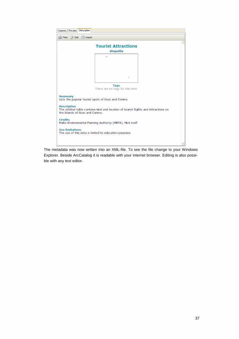
Catalog display
Tool Edit metadata
Click the button to open the Item Description of ‘Attrac-
tions’ . In the <Title> window type Tourist Attractions. In the
textbox next to <Summary (Purpose):> type Lists the popu-
lar tourist spots of Gozo and Comino. Click inside the text-
box next to <Description (Abstract):> to place a descriptive
text. Type beneath <Credits> Malte Environmental Planning
Authority (MEPA) and MLA staff and limit the use of this
data beneath <Use Limitation> to education purposes.
Click Save to apply the changes and close the Editing
‘Attractions’ dialog.
37
The metadata was now written into an XML-file. To see the file change to your Windows
Explorer. Beside ArcCatalog it is readable with your internet browser. Editing is also possi-
ble with any text editor.

38
2 Advanced I
2.1 Tables
Every feature class no matter if it contains points, polylines or polygons is connected with an attribute
table. The content of the attribute table depends on the needs of the creator. On principle every entry
is imaginable: text, numbers and even hyperlinks to pictures or web pages.
Structure of tables
Inside ArcGIS table rows are called records and columns are called fields. A field is defined by its
name, its field type and its width. All features of a dataset - means all records - share the same fields
or attributes.
No matter which data format you use the attribute table has to contain a field that stores the geo-
graphical information. In ArcGIS this is the field Shape. It will be created automatically as well as the
field FID with a numbering for the program intern organization of the features. In your attribute table
the field Shape appears with an entry that specifies whether your dataset stores points, lines or
polygons.
Normally every record belongs to one geographical feature of the dataset in your map. They are
dynamically linked each other. If you select a feature in your map the corresponding record in your
table will be highlighted, if you make a selection in your attribute table the linked features in your map
will be highlighted.
Like in a database there could be relationships between tables. Depending on the goal tables can be
linked or joined using a key field.
39
2.2 Exercise Analyze data
Task
The strength of GIS consists not only in display but in analyzing and querying your data. For an
agricultural report you want to query your existing data, create a statistic about the different kinds of
using the fields and their share of the whole area.
Moreover there was an inquiry whether viticultural fields are situated near a main road and which
kind of fields lay inside a 50 meters buffer of the main roads.
Data
The needed data are the streets layer and the agricultural use - both come from the MEPA - and the
topographic map of Gozo in the scale 1:25.000 as png-file.
Used functions
Identifying and symbolizing data
Prepare tables appearance
Calculate field values
Create statistics
Select features by attribute
Select features by location
How to do this
1. Prepare your data frame
Start the program if necessary, create a new map document and add some data.
Windows Double-click the ArcMap icon on your desktop or click the
Start button and point to <Programs>, <ArcGIS> and
<ArcMap> to launch ArcMap.
Choose blank map from the ArcMap dialog.
TOC Set the properties of your data frame by right-click on the
data frame name (Layers) and point to Properties…. In the
Data Frame Properties choose the General tab, rename
your data frame to Analysis and choose Meters for map and
display units. When you have done so click OK to close the
Data Frame Properties dialog.
Standard toolbar
Tool Add Data
From <personalfolder>/exercise/shape/… add the layer files
Roads.lyr, Islands.lyr and Agricultural Use.lyr you created in
former exercises and the shapefile dev_zone.shp to your
map. For a better orientation add the topographical map
malta_25.png from <personalfolder>/exercise/im-
ages/topmap… to the map.
40
TOC
Layer malta_25.png
To use the topographical map as an orientation layer the
representation should be changed to transparent. Right-click
at the layer name, point to properties, choose the Display
tab and enter 50 % next to <Transparency>.
Choose the General tab and rename your layer next to
<Layer Name:> to TopMap.
Click OK to close the Layer Properties and apply your
changes.
TOC Bring your layers into the following order (from top): Islands,
TopMap, Roads, DEV_ZONE, Agricultural Use.
! Remove the no longer needed transparency for your layer Islands. Furthermore change the
name of your layer DEV_ZONE to Settlements.
Standard toolbar
Tool Save
Save your map document as Exercise2-2.mxd in your <per-
sonalfolder>/exercise/projects/….
2. Identify and symbolize data
The simplest way to get information about a feature is to identify it with a suitable tool as
you have done in former exercises.
Tools toolbar
Tool Identify
Click on any feature that belongs to your layer Settlements.
Probably the wrong feature blinks short then the Identify
window pops up and shows the result from the top-most
layer. Because you are interested not in that layer you
change the layer next to <Identify from:> to Settlements.
Keep the window opened and repeat clicking the feature.
Again the selected feature blinks once green and the Identi-
fy window shows the attributes of the feature. E. g. next to
the field FEATURE you can find out whether it is an urban or
industrial area.
Close the Identify window.
A simple but often not distinct way to get information about a feature is how you symbol-
ized it. Your layers Roads and Agricultural Use are already useful symbolized. For Settle-
ments you do it yourself.
TOC
Layer Settlements
Right-click on your layer Settlements, point to Properties…
and choose the Symbology tab if necessary.
In the left box beneath <Show:> change from Fea-
tures/Single Symbol to Categories/Unique Values. Choose
from the drop-down list next to <Value Field> FEATURE and
add all values using the appropriate button on the bottom of
the Layer Properties window. Accept the randomly chosen
colors by clicking OK.
To get information about more than one feature of the attribute table you can combine
them for symbolizing. For example you are interested in the names of the settlements and
their belonging to urban or industrial areas.
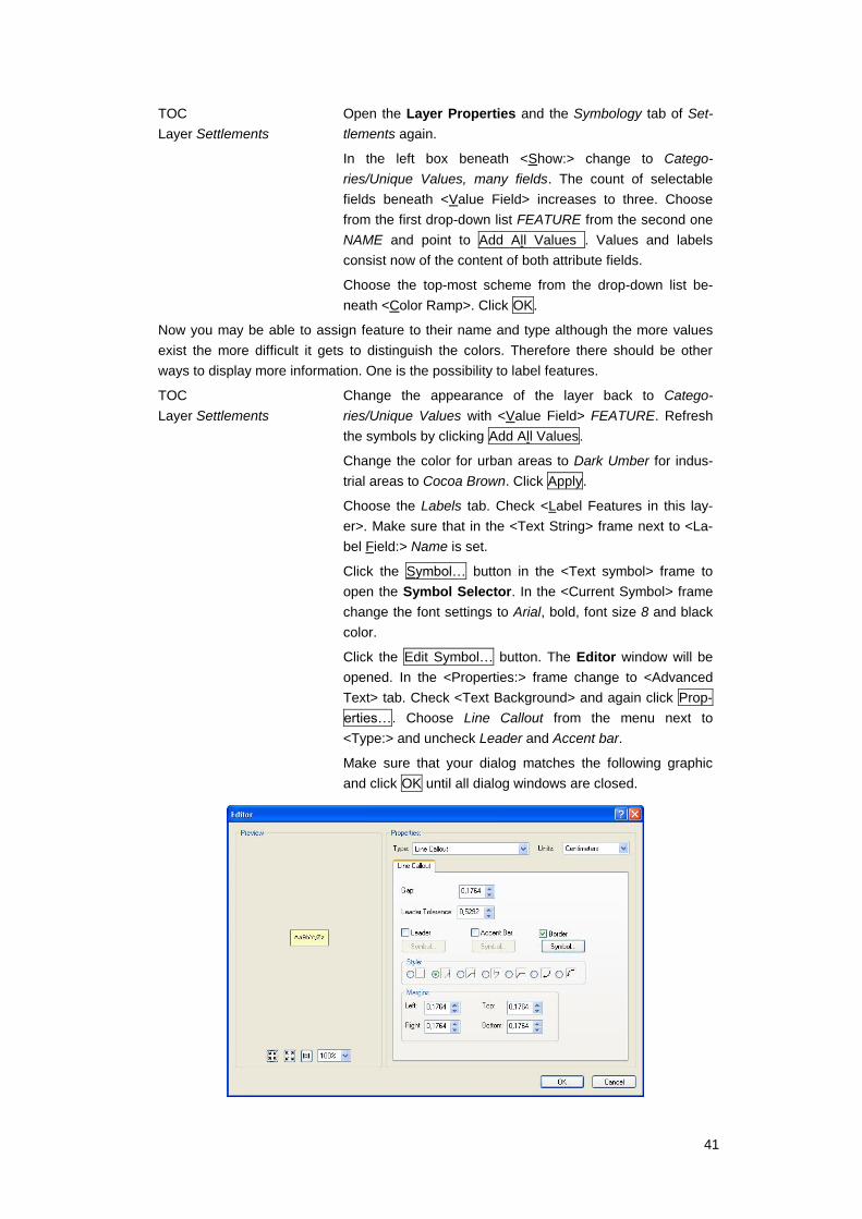
41
TOC
Layer Settlements
Open the Layer Properties and the Symbology tab of Set-
tlements again.
In the left box beneath <Show:> change to Catego-
ries/Unique Values, many fields. The count of selectable
fields beneath <Value Field> increases to three. Choose
from the first drop-down list FEATURE from the second one
NAME and point to Add All Values . Values and labels
consist now of the content of both attribute fields.
Choose the top-most scheme from the drop-down list be-
neath <Color Ramp>. Click OK.
Now you may be able to assign feature to their name and type although the more values
exist the more difficult it gets to distinguish the colors. Therefore there should be other
ways to display more information. One is the possibility to label features.
TOC
Layer Settlements
Change the appearance of the layer back to Catego-
ries/Unique Values with <Value Field> FEATURE. Refresh
the symbols by clicking Add All Values.
Change the color for urban areas to Dark Umber for indus-
trial areas to Cocoa Brown. Click Apply.
Choose the Labels tab. Check <Label Features in this lay-
er>. Make sure that in the <Text String> frame next to <La-
bel Field:> Name is set.
Click the Symbol… button in the <Text symbol> frame to
open the Symbol Selector. In the <Current Symbol> frame
change the font settings to Arial, bold, font size 8 and black
color.
Click the Edit Symbol… button. The Editor window will be
opened. In the <Properties:> frame change to <Advanced
Text> tab. Check <Text Background> and again click Prop-
erties…. Choose Line Callout from the menu next to
<Type:> and uncheck Leader and Accent bar.
Make sure that your dialog matches the following graphic
and click OK until all dialog windows are closed.

42
Tools toolbar
Tool Zoom in
Drag a rectangle around the northwest quarter of Gozo to
zoom there.
Some of the settlements consist of more than one part (especially Ghasri). To avoid multi-
ple labels change the settings of the label again.
TOC
Layer Settlements
Reopen the Layer Properties and choose the Labels tab if
necessary. In the <Other Options> frame click Placement
Options…. In the Placement Properties choose the
Placement tab.
In the <Duplicate Labels> frame on the bottom of the win-
dow check <Remove duplicate labels>.
Click OK to close the Placement Properties and again OK
to close the Layer Properties.
Tools toolbar
Tool Full extent
When you zoom to the full extent your label boxes cover the
other layers because of their size.
! Set a reference scale 1:50.000 to scale your labels. Exclude the Roads layer from scaling.
Another way to provide the user with information about features is to give map tips. Map
tips pop-up when you move the mouse cursor over a feature. For your layer Agricultural
Use map tips are already set which show the entry of the attribute field SUMMARY_DE,
but actually you are more interested in tips about the islands names.
TOC
Layer Agricultural Use
Open the Layer Properties by double-click the layer name
and choose the Display tab if necessary. Uncheck <Show
Map Tips using the display expression>.
Click OK to close the Layer Properties.
TOC
Layer Islands
Switch to the Display tab. Check <Show Map Tips using the
display expression> and choose out of the drop-down list
next to <Field> Maltese_Na. Click OK to apply your chang-
es. Examine your settings by moving the cursor over the
islands.
3. Change tables appearance
Tables may contain a lot of columns that are not very useful for you when you are looking
for special entries. You can hide recently not needed columns as well as change the order
of the size of columns. The changes have no influence on your table on the disc but only
inside your map document.
TOC
Layer Agricultural Use
Right-click on the layer name and point to Open Attribute
Table.

43
Attribute table of
Agricultural Use
Scroll to the right to get an overview to all fields. One im-
pression you may get is that many of the fields are momen-
tary empty and only the field SUMMARY_DE contains help-
ful information. Scroll to this field. Right-click into the field
heading and point to Freeze/Unfreeze column. The column
switches to the left edge of the table and remains there, no
matter if you scroll to the left or to the right.
By clicking on its right black bar and dragging you can re-
duce the column width. Do it for all the headings to a neces-
sary degree especially for these of the fields FEATURE and
SOURCE.
To hide columns you have to go to the layer properties.
Attribute table of
Agricultural Use
Drag your table to the side so that you can see the TOC.
TOC
Layer Agricultural Use
Double-click on the layer name to open its properties.
Choose the <Fields> tab. A box lists you the whole table
fields and their properties. In the frame <Choose which
fields will be visible> click on the field AGRI_ID. It will be
marked with a blue background. Beside the name uncheck
the box for this field. In your map document the field
AGRI_ID is no longer visible when you open the table or
identify a feature. Repeat the last step for the fields GEN-
ERAL_CO, DETAILED_C, REF_NO, REF_TYPE, CATE-
GORY, TYPE, REPORT_REF, SOURCE, PLOTTED_BY,
FILE_SAVE_ to hide them all.
Because SUMMARY_DE is not really descriptive about the
field content we give an alias for it. Select the field SUM-
MARY_DE and replace the text next to <Alias:> (beside the
list) with CULTIVATION.
Click OK to close the properties.
Attribute table of
Agricultural Use
Because there are only some fields left the freezing of the
renamed field CULTIVATION is no longer needed. Right-
click on the field heading and point to Freeze/Unfreeze
Column. The black bar on the right edge of the column
vanishes but the field remains on the most-left position.
Click in the heading and drag the column right of the field
FEATURE. A red bar shows the position while you drag it.
Close the table.
Check the result of your last actions.
Tools toolbar
Tool Identify
Click on any field on the islands. In the pop-up window
Identify change the identified layer next to <Identify from:>
to Agricultural Use. Click again any feature. The result
should show only the remaining and partly renamed fields.
Close the window.

44
4. Calculate values
A strength of GIS consists in its ability of a quick supply of values like area of polygons or
length of polylines. In a previous exercise you already calculated the area of the layer
Islands. Furthermore we need for our analysis the length of the roads and the areas of our
agricultural fields.
TOC
Layer Roads
Right-click on the layer name and point to Open Attribute
Table.
Attribute table of Roads Point to Table Options and click Add Field…. In the Add
Field dialog name the field Length_km, choose the <Type:>
Double and click OK. The new attribute field is added at the
end of the table. You may have to scroll to the right to see it.
As its name suggests we should calculate the values in
kilometers.
Make sure that no record is selected in your table because
otherwise the calculation would only be made for the select-
ed records. You find information about it on the bottom of
the table. If there is one or more record selected point to
Table Options and click Clear Selection.
Attribute table of Roads Right-click the heading for the new created field Length_km
and point to Calculate Geometry…. Confirm the warning to
get the Calculate Geometry opened. Click <OK>.
Right-click again the heading of the field Length_km and
point to Field Calculator… and insert following expression in
the text box beneath <Length_km=> [Length_km]/1000.
Click <OK>.
The Field Calculator converts now the length from Meters
into Kilometers.
Right-click the field heading and point to Sort Ascending.
Scroll up and down and view the largest and smallest road
parts.
As you could see there are three parts with 0 for length. Probably these parts result from
faulty digitizing and – because of their not existing length - are no longer necessary. To
delete these from the table you have to be in an edit session.
Attribute table of Roads Move your table that you can see the menus and toolbars.
Standard toolbar
Tool Editor toolbar
Open the Editor Toolbar if necessary.
Editor Toolbar,
Menu Editor,
Command Start Editing
Start the edit session for the layer Roads and go back to the
attribute table of your layer Roads.
45
Attribute table of Roads Select the three records you wish to delete by clicking on
the gray box left of the record. To select more than one
record either press the CTRL-key or keep the mouse clicked
and drag it over the three boxes. Press the DEL-key to
delete the records.
Editor Toolbar,
Menu Editor,
Command Stop Editing
Finish your edit session and click Yes to save your changes.
Standard toolbar
Tool Editor toolbar
Close the Editor Toolbar.
Attribute table of Roads Go back to your table. Right-click on the heading of your
field Length_km and point to Statistics. A statistic window
opens and shows beside others the shortest and longest
digitized part, the average length and the sum.
! Create a new field called Area in the attribute table of your layer Agricultural Use. Calculate
the area for it and convert it into square km.
5. Join tables
The attribute table of your layer Roads contains a field called FEATCO with coded values
about the road types. In another table the description for the codes are stored. A join
makes available the description in your attribute table of the layer Roads.
Standard toolbar
Tool Add Data
Browse your <personalfolder>/exercise/table for the table
Roadcodes.dbf, select it and click Add.
The table is added to your table of content. To see it in the TOC its mode switches auto-
matically to List by Source tab on the top of it.
TOC
Table Roadcodes
Right-click on the table name and point to open. View the
content of the table. Afterwards close the table.
TOC
Layer Roads
Right-click on the table name, point to Joins and Relates
and click Join…. The Join Data dialog will be opened.
Make sure that Join attributes from a table is chosen from
the first drop-down menu.
In the first step choose the field FEATCO from the drop-
down list. In the second box choose Roadcodes from the
list. Enter the field you want to use for joining in step 3. It
should be the field Code. When your dialog matches the
following graphic click OK.
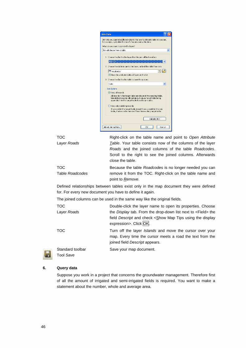
46
TOC
Layer Roads
Right-click on the table name and point to Open Attribute
Table. Your table consists now of the columns of the layer
Roads and the joined columns of the table Roadcodes.
Scroll to the right to see the joined columns. Afterwards
close the table.
TOC
Table Roadcodes
Because the table Roadcodes is no longer needed you can
remove it from the TOC. Right-click on the table name and
point to Remove.
Defined relationships between tables exist only in the map document they were defined
for. For every new document you have to define it again.
The joined columns can be used in the same way like the original fields.
TOC
Layer Roads
Double-click the layer name to open its properties. Choose
the Display tab. From the drop-down list next to <Field> the
field Descript and check <Show Map Tips using the display
expression>. Click OK.
TOC Turn off the layer Islands and move the cursor over your
map. Every time the cursor meets a road the text from the
joined field Descript appears.
Standard toolbar
Tool Save
Save your map document.
6. Query data
Suppose you work in a project that concerns the groundwater management. Therefore first
of all the amount of irrigated and semi-irrigated fields is required. You want to make a
statement about the number, whole and average area.

47
TOC
Layer Agricultural Use
Right-click on the layer name and point to Open Attribute
Table. In the attribute table scroll to the right to see the field
SUMMARY_DE (CULTIVATION). Right-click on the heading
and click Sort Ascending. Scroll down to find the records
with the appropriate entries.
You could now select them interactively by clicking all them in the table. Because there are
a lot of fields which are irrigated or semi-irrigated it is more comfortable to use a query.
TOC
Layer Agricultural Use
Point to Table Options on the bottom of the table and click
Select By Attributes…. The Select by Attributes dialog
appears.
To make a condition double-click a field, click an operator and double-click a value from
the giving lists or type parts of or the whole expression.
Select By Attributes dialog Make sure that Create a new selection is chosen from the
menu next to <Method:>.
Double-click ”SUMMARY_DE” from the list beneath
<Fields:>. It appears in the textbox in the lower part of the
dialog. From the middle of the dialog click the Equal opera-
tor ( = ). In the box right of the operators nothing is stated.
Click the Get Unique Values button to see all the values.
Afterwards double-click ‘IRRIGATED’ to get it from the list to
textbox below. The expression in the textbox should now be
“SUMMARY_DE” = ‘IRRIGATED’. Click Verify to check
whether your expression is all right. Depending on the result
of the verifying either correct your expression or continue by
clicking Apply.
TOC
Layer Agricultural Use
The table switches to the foreground. On the bottom of it you
can read that 594 of the 4889 records are selected. Switch
back to the Select By Attributes dialog.
Currently only the irrigated fields are selected. In fact you want to select all the records
which are either irrigated or semi-irrigated. To insert more than on criteria you have to
combine your single conditions with the operators <AND> or <OR>.
Select By Attributes dialog Continue the expression in your dialog by clicking the ap-
propriate elements of the box. The expression has to look
like the following statement:
"SUMMARY_DE" = 'IRRIGATED' OR "SUMMARY_DE" =
'SEMI-IRRIGATED'.
Again Verify your expression and in case of a successful
expression Apply it. Close the Select By Attributes dialog.

48
TOC
Layer Agricultural Use
Scroll down to see the selected records. To view only the
selected records click Show Selected Records on the bot-
tom of the table.
Scroll to the right to see the column AREA on the right edge
of the table. Right-click on the heading and point to Statis-
tics…. The Selection Statistics of AGRI window states
besides others the count of the fields, the sum of the area
and the mean area.
After you have examined the statistic you can close it.
For your analysis you are only interested in the irrigated fields which are bigger than
10.000 square meters.
TOC
Layer Agricultural Use
Again point to Table Options in the menü of the table and
click Select By Attributes….
Select By Attributes dialog Change the selection <Method:> to Select from current
selection. Clear any expression if necessary.
Create a new expression "Area_km" > 10, Verify and Apply
it. Because of the changed selection method only records
from the existing selection will be queried.
7. Summaries
A more durable way of statistic is to create a summary. Because you were asked to create
a statistic about the agricultural use you want to create a new table with these information.
TOC
Layer Agricultural Use
On the bottom of the table choose all records by clicking the
Show all Records button. Afterwards point to Table Options
and click Clear Selection. The status bar on the bottom of
the table should now state that no record is selected.
Scroll horizontal to get the SUMMARY_DE (Cultivation)
field. Right-click on the heading and point to Summarize….
Summarize dialog In the Summarize dialog make sure that SUMMARY_DE is
set for field in the first step.
For summary statistics select from the offered list the
summed area, the first feature and the first contact_pe. To
do so click the plus next to Area_km and check <Sum>. For
FEATURE and CONTACT_PE check <First>.
In the third step navigate to your folder tables and name the
table Sum_agri.dbf. Make sure that the dialog matches the
following graphic then click OK. Click Yes when prompted
to add the table to your map.
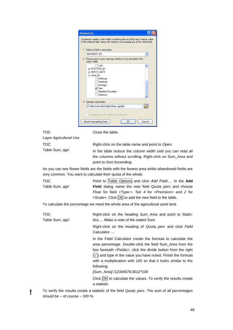
49
TOC
Layer Agricultural Use
Close the table.
TOC
Table Sum_agri
Right-click on the table name and point to Open.
In the table reduce the column width until you can read all
the columns without scrolling. Right-click on Sum_Area and
point to Sort Ascending.
As you can see flower fields are the fields with the fewest area whilst abandoned fields are
very common. You want to calculate their quota of the whole.
TOC
Table Sum_agri
Point to Table Options and click Add Field…. In the Add
Field dialog name the new field Quota_perc and choose
Float for field <Type:>. Set 4 for <Precision> and 2 for
<Scale>. Click OK to add the new field to the table.
To calculate the percentage we need the whole area of the agricultural used land.
TOC
Table Sum_agri
Right-click on the heading Sum_Area and point to Statis-
tics…. Make a note of the stated Sum.
Right-click on the heading of Quota_perc and click Field
Calculator….
In the Field Calculator create the formula to calculate the
area percentage. Double-click the field Sum_Area from the
box beneath <Fields>, click the divide button from the right
( / ) and type in the value you have noted. Finish the formula
with a multiplication with 100 so that it looks similar to the
following:
[Sum_Area] /12345678.9012*100
Click OK to calculate the values. To verify the results create
a statistic
! To verify the results create a statistic of the field Quota_perc. The sum of all percentages
should be – of course – 100 %.

50
8. Creating graphs
Main Menu View
Graphs
Command Create…
Open Create Graph Wizard.
In step 1 select Vertical Bar for <Graph Type> and make
sure that Sum_agri is chosen at <Layer/Table>. Choose out
of the drop-down list next to <Value Field> Quota_perc and
next to <X label field> SUMMARY_DE. For <Color> chose
Palette and Classic and click <Next>.
In step 2 type into the window next to <Title> in the <Gen-
eral graph properties> frame Agricultural Use and check the
box <Graph in 3D view>. Make sure that the box for the
<Graph legend> frame is checked. Beneath the <Axis prop-
erties> click the tab Left and type Percentage for <Title>.
For the tab Bottom make sure that the box for <Visible> is
unchecked and click <Finish>.
A graph window pops up that shows the just created diagram. Afterwards you can still
change some properties of it by right-click on the title bar of the window and and the
command Properties….
The diagram should look like the following graphic.
Graph Agricultural Use Close the Graph by clicking the cross sign in the upper right
corner. The graph is stored in your map document and can
be reopened over the main menu View with the command
Graphs.
TOC Change the TOC view from List By Source to List By Draw-
ing Order using the appropriate tab on the top of the TOC.
9. Spatial queries
The goal for the agricultural report you have to create was to examine whether viticultural
fields are situated near any main road. To analyze this you have to combine attribute and
location queries. First you have to select the main roads. These are the features of the
layer roads which have the entry W35 or W36 in the column FEATCO.
Tools toolbar
Tool Full extent
Zoom to the full extent of your map (only necessary if you
have changed the extent of your map view before).

51
Main Menu Selection
Select by Attributes…
Open the Select By Attributes dialog. Choose Roads for
<Layer:>. Make sure that Create a new selection is chosen
next to <Method:>.
All columns of the original attribut table from Roads have
now the prefix STR., columns of the joined table roadcodes
got the prefix roadcodes. That happened automatic and
shouldn’t bother you.
Create the expression "STR.FEATCO" LIKE 'W35' by dou-
ble-click the appropriate elements from the boxes.
Because of the two types of main roads replace the numeral
5 with a wildcard. When your expression matches the fol-
lowing "STR.FEATCO" LIKE 'W3_' all records will select
whose FEATCO starts with W3 no matter which character
follows.
Verify your expression and in case of a success Apply it.
Afterwards Close the Select By Attributes dialog. You
should now see the main roads blue highlighted in your
map.
Main Menu Selection
Select by Location…
Open the Select By Location dialog to define the spatial
query.
Make sure that select features from is chosen next to <Se-
lection method:>. Check the layer Agricultural Use from the
next list. As <Source layer> select Roads, make sure that
the box <use selected features> is checked.
From the <Spatial selection method> box choose Targed
layer(s) features are within a distance of the Source layer
feature.
Check <Apply a search distance> if necessary and enter a
buffer of 20 Meters in the last two textboxes.
When your dialog matches the following graphic click Apply
to run your spatial query and afterwards Close to close the
dialog.
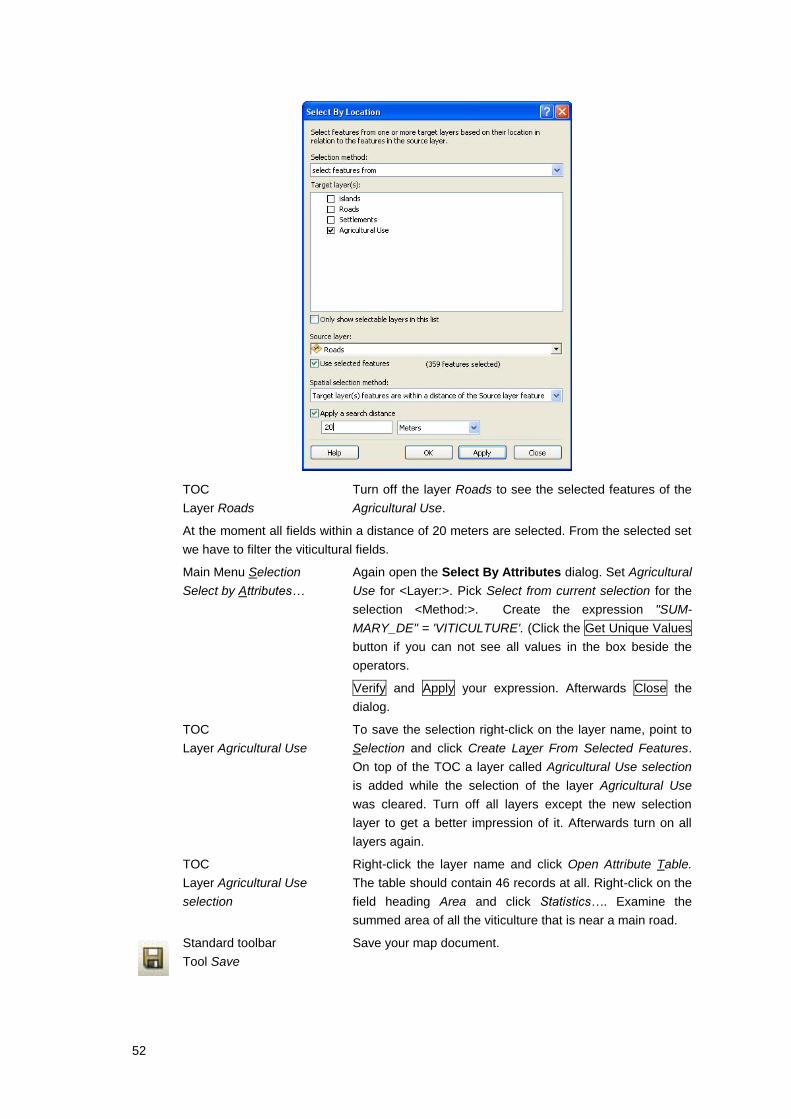
52
TOC
Layer Roads
Turn off the layer Roads to see the selected features of the
Agricultural Use.
At the moment all fields within a distance of 20 meters are selected. From the selected set
we have to filter the viticultural fields.
Main Menu Selection
Select by Attributes…
Again open the Select By Attributes dialog. Set Agricultural
Use for <Layer:>. Pick Select from current selection for the
selection <Method:>. Create the expression "SUM-
MARY_DE" = 'VITICULTURE'. (Click the Get Unique Values
button if you can not see all values in the box beside the
operators.
Verify and Apply your expression. Afterwards Close the
dialog.
TOC
Layer Agricultural Use
To save the selection right-click on the layer name, point to
Selection and click Create Layer From Selected Features.
On top of the TOC a layer called Agricultural Use selection
is added while the selection of the layer Agricultural Use
was cleared. Turn off all layers except the new selection
layer to get a better impression of it. Afterwards turn on all
layers again.
TOC
Layer Agricultural Use
selection
Right-click the layer name and click Open Attribute Table.
The table should contain 46 records at all. Right-click on the
field heading Area and click Statistics…. Examine the
summed area of all the viticulture that is near a main road.
Standard toolbar
Tool Save
Save your map document.

53
! Find out the length of the gravel roads which run through settlements. Start by making a
spatial query of all roads that are completely within the layer Settlement. After that reduce
the selection of your roads to those which are gravel roads (roads with the code W04 in the
field FEATCO). For this use an attribute query. Finally make a statistic of the field Length
to see the summed length of all the selected features. If the sum states 2,153434 km your
queries were all right.
54
2.3 Exercise Georeferencing
Task
If you want to create a vector layer you often use on-screen digitizing based on an existing raster
image. Scanned raster data contain no digital readable information where the data is situated. You
can provide your data with this information by georeferencing.
For your map of Gozo and Comino you want to add data about geology. The analog base map was
scanned, is now available without any spatial reference and ready for georeferencing.
The geological information has to be vectorized to use it in an appropriate form. In ArcGIS/ArcView
vector data can be stored either as shapefile or as feature class inside a geodatabase. The geodata-
base offers some advantages such as the storage of lines, points, polygons in one file, the possibility
of defining topologically associated feature classes (spatial dependence), the storage of annotations
and the possible definition of rules (e. g. domains) for attribute values. Therefore we want to use the
geodatabase to create a new feature class geology and digitize the geological formations on your
screen. Moreover we want to add other existing data to the geodatabase.
Data
Available is the scanned but not georeferenced geological map of Gozo and Comino as jpg-file and
the topographic map of Gozo in the scale 1:25.000 as png-file already with spatial reference. Moreo-
ver there are all the data you had used or created before.
Used functions
Georeferencing
Create a geodatabase
Work with domains
Import data to your geodatabase
Modify features
How to do this
1. Georeference an image
Start the program, create a new map document and add some data.
Windows Double-click the ArcMap icon on your desktop or click the
Start button and point to Programs - ArcGIS - ArcMap to
launch ArcMap.
ArcMap dialog
Blank Map
Create a new empty document.
Set the properties of your new empty data frame.
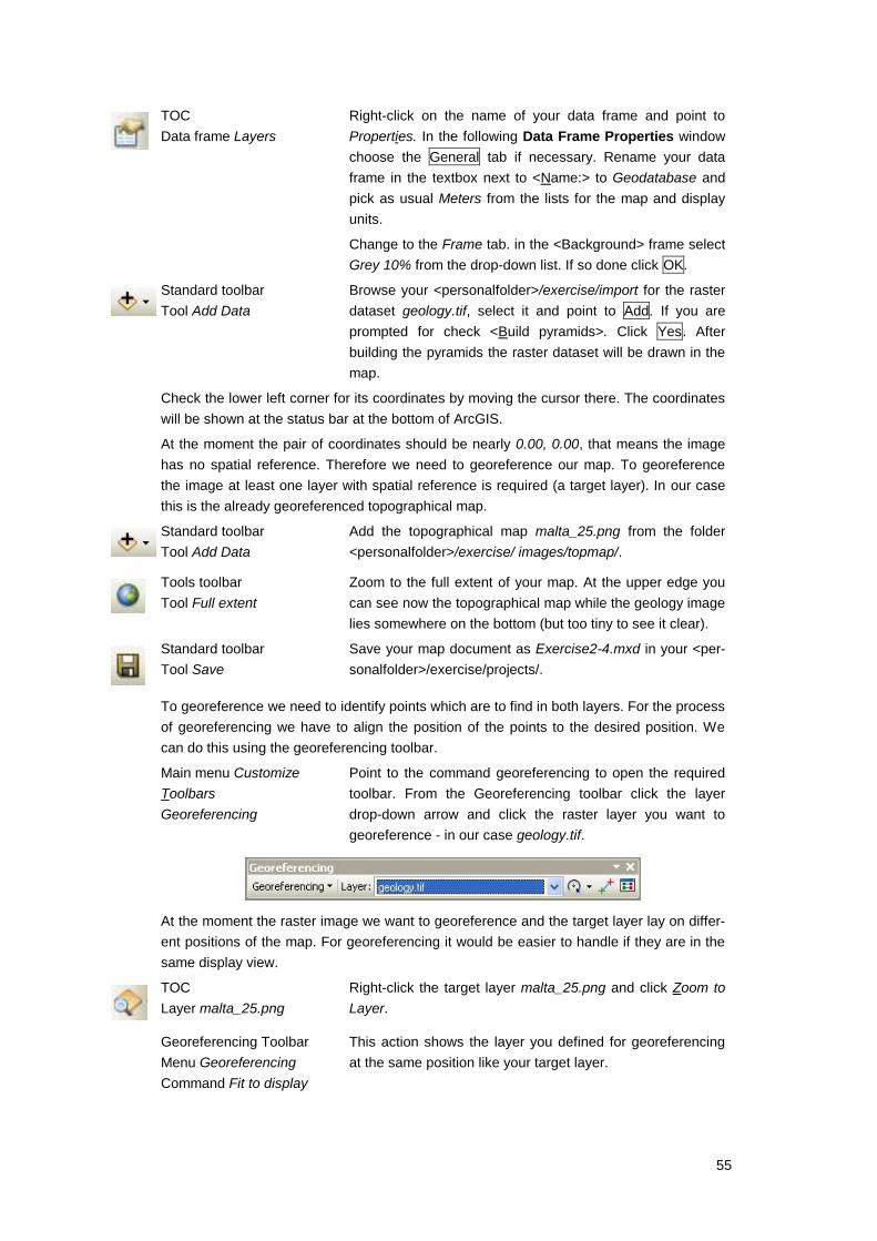
55
TOC
Data frame Layers
Right-click on the name of your data frame and point to
Properties. In the following Data Frame Properties window
choose the General tab if necessary. Rename your data
frame in the textbox next to <Name:> to Geodatabase and
pick as usual Meters from the lists for the map and display
units.
Change to the Frame tab. in the <Background> frame select
Grey 10% from the drop-down list. If so done click OK.
Standard toolbar
Tool Add Data
Browse your <personalfolder>/exercise/import for the raster
dataset geology.tif, select it and point to Add. If you are
prompted for check <Build pyramids>. Click Yes. After
building the pyramids the raster dataset will be drawn in the
map.
Check the lower left corner for its coordinates by moving the cursor there. The coordinates
will be shown at the status bar at the bottom of ArcGIS.
At the moment the pair of coordinates should be nearly 0.00, 0.00, that means the image
has no spatial reference. Therefore we need to georeference our map. To georeference
the image at least one layer with spatial reference is required (a target layer). In our case
this is the already georeferenced topographical map.
Standard toolbar
Tool Add Data
Add the topographical map malta_25.png from the folder
<personalfolder>/exercise/ images/topmap/.
Tools toolbar
Tool Full extent
Zoom to the full extent of your map. At the upper edge you
can see now the topographical map while the geology image
lies somewhere on the bottom (but too tiny to see it clear).
Standard toolbar
Tool Save
Save your map document as Exercise2-4.mxd in your <per-
sonalfolder>/exercise/projects/.
To georeference we need to identify points which are to find in both layers. For the process
of georeferencing we have to align the position of the points to the desired position. We
can do this using the georeferencing toolbar.
Main menu Customize
Toolbars
Georeferencing
Point to the command georeferencing to open the required
toolbar. From the Georeferencing toolbar click the layer
drop-down arrow and click the raster layer you want to
georeference - in our case geology.tif.
At the moment the raster image we want to georeference and the target layer lay on differ-
ent positions of the map. For georeferencing it would be easier to handle if they are in the
same display view.
TOC
Layer malta_25.png
Right-click the target layer malta_25.png and click Zoom to
Layer.
Georeferencing Toolbar
Menu Georeferencing
Command Fit to display
This action shows the layer you defined for georeferencing
at the same position like your target layer.
56
TOC
Layer malta_25.png
Double-click the layer name to open its properties. Click the
Display tab. Type a transparency of 30 % in the appropriate
textbox. Click OK.
To get more accurate results you can use a magnifier to zoom in the area of interest.
Menu Window
Command Magnifier…
A Magnification window appears. In the title you see the
factor of magnification. To change it right-click inside the title
and point to Properties…. Inside the <Zoom> frame enter
300 next to <Modify main view by>, press the Return key
and click OK. The new factor appears in the title.
To use a magnified view drag the Magnification window to
the area you are interested in. A cross-wires shows the
present location.
The basic procedure for georeferencing is to set links between raster and target layer. A
link means to set prominent points or points of known x,y coordinates in both raster and
target layer. Such prominent points could be a cape or the crossing of two roads or - more
accurate - a coordinate raster. To have at least one link near each corner of the raster and
a few throughout the interior produces the best results.
Georeferencing Toolbar
Tool Control points
Set a link using a mouse-click on a prominent point of your
raster geology.tif and the second click at its location at the
target layer. Well suited for such links are the coordinate
crossings on both layers. A better sight on the points you will
get if you turn off all layers except of this one you will just
work with.
After you have set a pair of linked points the map moves a
little.
Tools toolbar
Navigation tools
After setting a pair of points zoom to the fuel extent to look
for the next suited location. Because the maps match better
after every set pair of points you can use a bigger scale for
further points. Try to set points at a scale of about 1:15.000.
Additional you can enlarge the magnification zoom to a
zoom factor of 500 or even 800.
Georeferencing Toolbar
Tool Control points
Repeat to set links until you have a more or less regular
point cloud on your map. At least you need three pairs of
points, but better results we will reach with ten or more links.
Georeferencing Toolbar
Tool View Link Table
Open the Link Table. It shows the accuracy of your set
links. The residual error shows the error for each link, the
RMS the entire average error. For this you need at least four
points.
Tools toolbar
Tool Zoom In
A rough orientation for the RMS error gives the raster reso-
lution of your target layer and the layer you are just georef-
erencing on its target position. To get their resolutions zoom
in as far you can recognize the raster cells. This should be a
scale around 1:250.
Tools toolbar
Tool Measure
Measure the extent of a single cell in both your layer geolo-
gy.tif and the layer malta_25.png.
57
Georeferencing Toolbar
Tool View Link Table
Reopen the Link Table if necessary. Compare the <Total
RMS Error> with the raster resolution. It should not be big-
ger than the higher cell width of both of your measured
layers but even better half of it.
To improve the <Total RMS Error> you can delete links with
a high residual error from your table. To do so select the link
by clicking on it. It will be highlighted in yellow in your map.
Afterwards point to the Delete button ( x ) on the upper right
hand corner of your window to delete the link.
Add and delete links until your are satisfied with the <Total
RMS Error>. Click OK to close the Link Table.
Georeferencing Toolbar
Menu Georeferencing
Command Rectify…
The command Rectify… calculates a new georeferenced
raster image. In the appearing Save As dialog click the
folder button next to the textbox beneath <Output raster:>.
Browse to your <personalfolder>\exercise\images\… and
<Name:> the new raster geo_rec and choose as <Format:>
TIFF. Make sure that Nearest Neighbor is chosen for
<Resample Type:> and keep the suggested <Cell Size:>.
Click Save. The new file will created.
Standard Toolbar
Tool Add Data
Add your created raster image geo_rec.tif to ArcMap.
TOC
Layer geology.tif
The layer geology.tif is no longer needed. Right-click on the
layer name and point to Remove.
! Check the success of the former process by comparing the accuracy of both layers. Set a
transparency if necessary.
Standard toolbar
Tool Save
Save your map document.

58
3 Advanced II
3.1 Exercise Geoprocessing with ModelBuilder
Task
Geoprocessing is the processing of geographic information, one of the basic functions of a geo-
graphic information system (GIS). It provides a way to create new information by applying an opera-
tion on existing data. Any alteration or information extraction you perform on your data involves a
geoprocessing task. It can be a task such as converting geograhic data to a different format, or it can
involve multiple tasks performed in sequence, such as those that clip, select, then intersect datasets.
Within ArcGIS you can perform geoprocessing tasks in a number of ways. In the following example
we would like to create a model that runs the sequence of geoprocessing tools. Creating a model
provides a way to run a sequence of geoprocessing tools by enabling you to string your tools togeth-
er in a visual diagramm. A model can be run again and again and you can alter parameter values to
experiment with different outcomes.
Your task in this exercise is to locate potential areas for a touristical project on Gozo Island. You’ll
create an new model incorporating the following three criteria:
1. The landuse for our potential areas should be abandoned areas.
2. We need flat areas, so the slope should be less than 15%.
3. The maximum distance to urban areas should be less than 500m, so that everybody could
walk there by feet.
Data
The vector data was created and made available by the Malta Environment and Planning Authority
(MEPA). The slope was calculated and reclassified by the MLA staff.
Used functions
Working with the ArcToolbox Environment
Creating a new Toolbox
Creating a new model
Running and debugging the model
Saving and document the model
How to do this
1. Opening the ArcMap and ArcToolbox window and setting workspaces
Start the program, create a new map document and add some data.
Windows Double-click the ArcMap icon on your desktop or click the
Start button and point to Programs - ArcGIS - ArcMap to
launch ArcMap.
ArcMap dialog
Blank Map
Create a new empty document.
Set the properties of your new empty data frame.

59
TOC
Data frame Layers
Right-click on the name of your data frame and point to
Properties. In the following Data Frame Properties window
choose the General tab if necessary. Rename your data
frame in the textbox next to <Name:> to Analysis and pick
as usual Meters from the lists for the map and display units.
If so done click OK.
Standard toolbar
Tool Add Data
Browse your <personalfolder>/exercise/shape for the vector
dataset agri.shp, slope.shp and dev_zone.shp, select it and
point to Add.
Tools toolbar
Tool Full extent
Zoom to the full extent of your map.
Standard toolbar
Tool Save
Save your map document as Analysis.mxd in your <person-
alfolder>/exercise/projects/.
Standard Toolbar
Tool Show/Hide ArcToolbox
Window
When working in ArcMap, you access toolboxes through the
ArcToolbox window. By saving the map document you save
any changes made to the ArcToolbox window. This allows
you to have different versions of the ArcToolbox window
with each map document you create, depending on which
tools you want to use for each project.
Click the Show/Hide ArcToolbox window. If the ArcToolbox
window does not display inside the ArcMap table of contents
window, click and drag the bar at the top of the ArcToolbox
window and place it over the top of the table of contents
window, then drop the panel.
The Arc Toolbox is now placed in the TOC window, you can
change between Arc Toolbox and TOC by selecting them
via tab on the bottom of the TOC window.
ArcToolbox window Right-click the ArcToolbox window and click environments.
Click the Workspace dropdown arrow. Click the Browse
button and check the location. Please use for the <Current
Workspace> <personalfolder>/exercise/shape and for
<Scratch Workspace> <personalfolder>/exercise. Click OK
ArcToolbox window Right-click the ArcToolbox window and create a New
Toolbox with the command Add Toolbox. In the Add
Toolbox window click the New Toolbox Tool and name the
Toolbox My_Analysis_Tools.
Standard toolbar
Tool Save
Save your map document. The Geoprocessing settings
include environment settings, the state of the ArcToolbox
window and variables you have created at the command
line. These settings are saved in the ArcMap document.
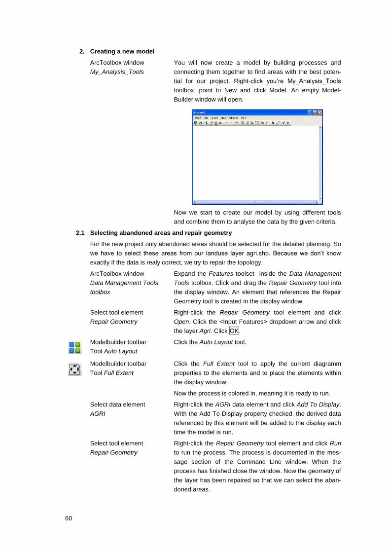
60
2. Creating a new model
ArcToolbox window
My_Analysis_Tools
You will now create a model by building processes and
connecting them together to find areas with the best poten-
tial for our project. Right-click you’re My_Analysis_Tools
toolbox, point to New and click Model. An empty Model-
Builder window will open.
Now we start to create our model by using different tools
and combine them to analyse the data by the given criteria.
2.1 Selecting abandoned areas and repair geometry
For the new project only abandoned areas should be selected for the detailed planning. So
we have to select these areas from our landuse layer agri.shp. Because we don’t know
exactly if the data is realy correct, we try to repair the topology.
ArcToolbox window
Data Management Tools
toolbox
Expand the Features toolset inside the Data Management
Tools toolbox. Click and drag the Repair Geometry tool into
the display window. An element that references the Repair
Geometry tool is created in the display window.
Select tool element
Repair Geometry
Right-click the Repair Geometry tool element and click
Open. Click the <Input Features> dropdown arrow and click
the layer Agri. Click OK.
Modelbuilder toolbar
Tool Auto Layout
Click the Auto Layout tool.
Modelbuilder toolbar
Tool Full Extent
Click the Full Extent tool to apply the current diagramm
properties to the elements and to place the elements within
the display window.
Now the process is colored in, meaning it is ready to run.
Select data element
AGRI
Right-click the AGRI data element and click Add To Display.
With the Add To Display property checked, the derived data
referenced by this element will be added to the display each
time the model is run.
Select tool element
Repair Geometry
Right-click the Repair Geometry tool element and click Run
to run the process. The process is documented in the mes-
sage section of the Command Line window. When the
process has finished close the window. Now the geometry of
the layer has been repaired so that we can select the aban-
doned areas.
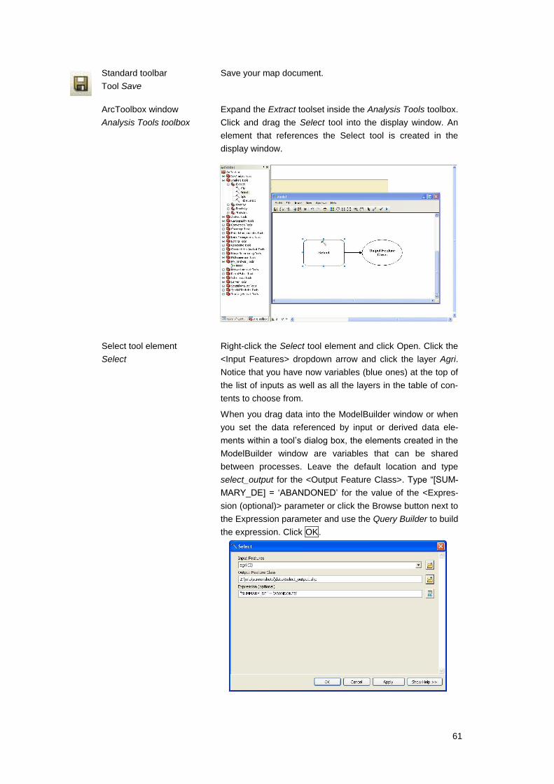
61
Standard toolbar
Tool Save
Save your map document.
ArcToolbox window
Analysis Tools toolbox
Expand the Extract toolset inside the Analysis Tools toolbox.
Click and drag the Select tool into the display window. An
element that references the Select tool is created in the
display window.
Select tool element
Select
Right-click the Select tool element and click Open. Click the
<Input Features> dropdown arrow and click the layer Agri.
Notice that you have now variables (blue ones) at the top of
the list of inputs as well as all the layers in the table of con-
tents to choose from.
When you drag data into the ModelBuilder window or when
you set the data referenced by input or derived data ele-
ments within a tool’s dialog box, the elements created in the
ModelBuilder window are variables that can be shared
between processes. Leave the default location and type
select_output for the <Output Feature Class>. Type “[SUM-
MARY_DE] = ‘ABANDONED’ for the value of the <Expres-
sion (optional)> parameter or click the Browse button next to
the Expression parameter and use the Query Builder to build
the expression. Click OK.

62
Modelbuilder toolbar
Tool Auto Layout
Click the Auto Layout tool.
Modelbuilder toolbar
Tool Full Extent
Click the Full Extent tool to apply the current diagramm
properties to the elements and to place the elements within
the display window.
Now the process is colored in, meaning it is ready to run.
Select data element
Agri_Select.shp
Right-click the Agri_Select.shp data element and click Re-
name. Type Abandoned Area and Click OK. Right-click the
Abandoned Area data element and click Add To Display.
With the Add To Display property checked, the derived data
referenced by this element will be added to the display each
time the model is run.
Select tool element
Select
Right-click the Select tool element and click Run to run the
process. The process is documented in the message sec-
tion of the Command Line window. When the process has
finished close the window. Minimize the ModelBuilder win-
dow.
TOC
Layer Abandoned Area
Examine the layer Abandoned Area in your ArcMap display.
Only the abandoned areas from the repaired layer agri.shp
have been selected.
Standard toolbar
Tool Save
Save your map document.
2.2 Selecting Suitable Areas with a slope less than 15% and repair geometry
Because it is too expensive to build in very steep areas we need to know where the slope
is less than 15%. So we have to select all these areas from our layer slope.shp. Before we
can start, we have to repair the geometry to make our analysis.
ArcToolbox window
Data Management Tools
toolbox
Expand the Features toolset inside the Data Management
Tools toolbox. Click and drag the Repair Geometry tool into
the display window.
Select tool element
Repair Geometry
Right-click the Repair Geometry tool element and click
Open. Click the <Input Features> dropdown arrow and click
the layer slope. Click OK.
Modelbuilder toolbar
Tool Auto Layout
Click the Auto Layout tool.
Modelbuilder toolbar
Tool Full Extent
Click the Full Extent tool to apply the current diagramm
properties to the elements and to place the elements within
the display window.
Select data element
slope
Right-click the slope data element and click Add To Display.
With the Add To Display property checked, the derived data
referenced by this element will be added to the display each
time the model is run.
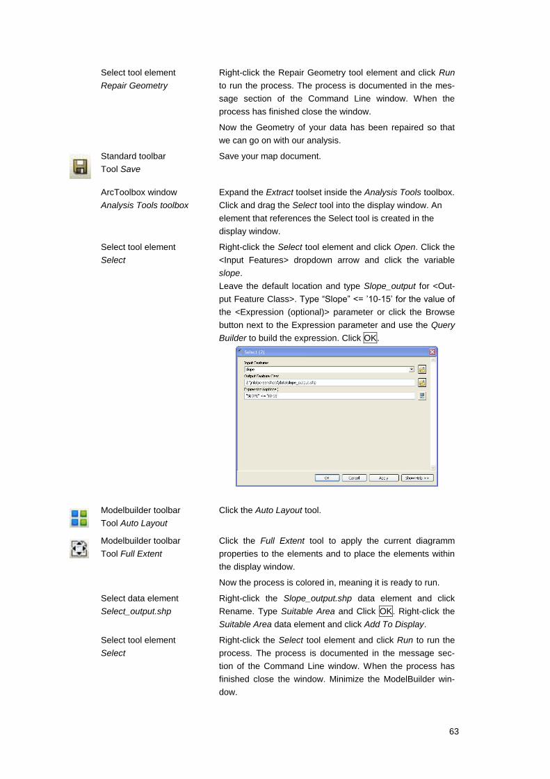
63
Select tool element
Repair Geometry
Right-click the Repair Geometry tool element and click Run
to run the process. The process is documented in the mes-
sage section of the Command Line window. When the
process has finished close the window.
Now the Geometry of your data has been repaired so that
we can go on with our analysis.
Standard toolbar
Tool Save
Save your map document.
ArcToolbox window
Analysis Tools toolbox
Expand the Extract toolset inside the Analysis Tools toolbox.
Click and drag the Select tool into the display window. An
element that references the Select tool is created in the
display window.
Select tool element
Select
Right-click the Select tool element and click Open. Click the
<Input Features> dropdown arrow and click the variable
slope.
Leave the default location and type Slope_output for <Out-
put Feature Class>. Type “Slope” <= ’10-15’ for the value of
the <Expression (optional)> parameter or click the Browse
button next to the Expression parameter and use the Query
Builder to build the expression. Click OK.
Modelbuilder toolbar
Tool Auto Layout
Click the Auto Layout tool.
Modelbuilder toolbar
Tool Full Extent
Click the Full Extent tool to apply the current diagramm
properties to the elements and to place the elements within
the display window.
Now the process is colored in, meaning it is ready to run.
Select data element
Select_output.shp
Right-click the Slope_output.shp data element and click
Rename. Type Suitable Area and Click OK. Right-click the
Suitable Area data element and click Add To Display.
Select tool element
Select
Right-click the Select tool element and click Run to run the
process. The process is documented in the message sec-
tion of the Command Line window. When the process has
finished close the window. Minimize the ModelBuilder win-
dow.
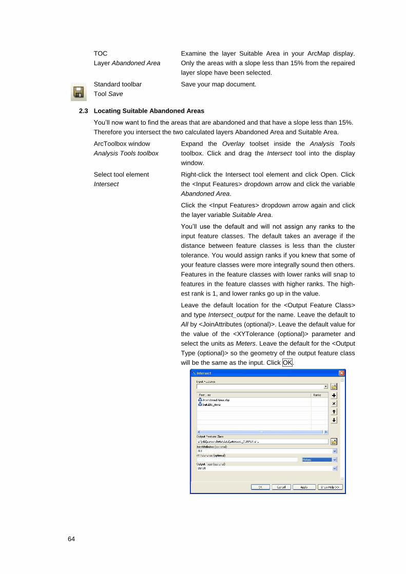
64
TOC
Layer Abandoned Area
Examine the layer Suitable Area in your ArcMap display.
Only the areas with a slope less than 15% from the repaired
layer slope have been selected.
Standard toolbar
Tool Save
Save your map document.
2.3 Locating Suitable Abandoned Areas
You’ll now want to find the areas that are abandoned and that have a slope less than 15%.
Therefore you intersect the two calculated layers Abandoned Area and Suitable Area.
ArcToolbox window
Analysis Tools toolbox
Expand the Overlay toolset inside the Analysis Tools
toolbox. Click and drag the Intersect tool into the display
window.
Select tool element
Intersect
Right-click the Intersect tool element and click Open. Click
the <Input Features> dropdown arrow and click the variable
Abandoned Area.
Click the <Input Features> dropdown arrow again and click
the layer variable Suitable Area.
You’ll use the default and will not assign any ranks to the
input feature classes. The default takes an average if the
distance between feature classes is less than the cluster
tolerance. You would assign ranks if you knew that some of
your feature classes were more integrally sound then others.
Features in the feature classes with lower ranks will snap to
features in the feature classes with higher ranks. The high-
est rank is 1, and lower ranks go up in the value.
Leave the default location for the <Output Feature Class>
and type Intersect_output for the name. Leave the default to
All by <JoinAttributes (optional)>. Leave the default value for
the value of the <XYTolerance (optional)> parameter and
select the units as Meters. Leave the default for the <Output
Type (optional)> so the geometry of the output feature class
will be the same as the input. Click OK.

65
Modelbuilder toolbar
Tool Auto Layout
Click the Auto Layout tool.
Modelbuilder toolbar
Tool Full Extent
Click the Full Extent tool to apply the current diagramm
properties to the elements and to place the elements within
the display window.
Select data element
Intersect_output.shp
Right-click the Intersect_output.shp data element and click
Rename. Type Intersect Output and Click OK. Right-click
the Intersect Output data element and click Add To Display.
Select tool element
Intersect
Right-click the Intersect tool element and click Run to run
the process. When the process has finished close the win-
dow. Minimize the Model Builder window.
TOC
Layer Intersect Output
Examine the layer Intersect Output in your ArcMap display.
Change the color to red. Now you can see all the areas that
are abandoned and have a slope less than 15%.
Standard toolbar
Tool Save
Save your map document.
2.4 Calculate zones round urban areas and exclude the Suitable Abandoned areas in-
side
You’ll now calculate the zones round urban areas in a defined distance, because people
living there should be able to go there by feet. First you have to buffer the urban areas
using a distance field in the attribute table, then clip the resultant buffer zones from the
Suitable abandoned areas.
ArcToolbox window
Analysis Tools toolbox
Expand the Proximity toolset inside the Analysis Tools
toolbox. Clik and drag the Buffer tool into the display win-
dow.
Select tool element
Buffer
Right-click the Buffer tool element and click Open. Click the
<Input Features dropdown> arrow and click the layer
DEV_ZONE.
Type for <Distance [value of field]> beneath Linear unit : 500
and click the drop-down arrow beside to choose Meters.The
values in this fields will be used for the width of the buffer.
Click the <Dissolve Type (optional)> dropdown arrow and
click LIST to list the Dissolve Fields. Click OK.
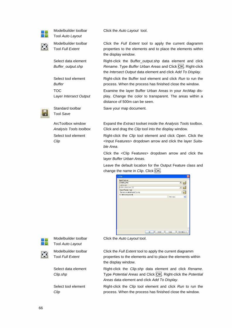
66
Modelbuilder toolbar
Tool Auto Layout
Click the Auto Layout tool.
Modelbuilder toolbar
Tool Full Extent
Click the Full Extent tool to apply the current diagramm
properties to the elements and to place the elements within
the display window.
Select data element
Buffer_output.shp
Right-click the Buffer_output.shp data element and click
Rename. Type Buffer Urban Areas and Click OK. Right-click
the Intersect Output data element and click Add To Display.
Select tool element
Buffer
Right-click the Buffer tool element and click Run to run the
process. When the process has finished close the window.
TOC
Layer Intersect Output
Examine the layer Buffer Urban Areas in your ArcMap dis-
play. Change the color to transparent. The areas within a
distance of 500m can be seen.
Standard toolbar
Tool Save
Save your map document.
ArcToolbox window
Analysis Tools toolbox
Expand the Extract toolset inside the Analysis Tools toolbox.
Click and drag the Clip tool into the display window.
Select tool element
Clip
Right-click the Clip tool element and click Open. Click the
<Input Features> dropdown arrow and click the layer Suita-
ble Area.
Click the <Clip Features> dropdown arrow and click the
layer Buffer Urban Areas.
Leave the default location for the Output Feature class and
change the name in Clip. Click OK.
Modelbuilder toolbar
Tool Auto Layout
Click the Auto Layout tool.
Modelbuilder toolbar
Tool Full Extent
Click the Full Extent tool to apply the current diagramm
properties to the elements and to place the elements within
the display window.
Select data element
Clip.shp
Right-click the Clip.shp data element and click Rename.
Type Potential Areas and Click OK. Right-click the Potential
Areas data element and click Add To Display.
Select tool element
Clip
Right-click the Clip tool element and click Run to run the
process. When the process has finished close the window.

67
TOC
Click all results except Potential Areas in the table of con-
tents, right-click and click Remove. Change the color of the
layer Potential Areas in red.
It shows all areas based on the criteria set.
Standard toolbar
Tool Save
Save your map document.
3 Saving and renaming the model
Any new model you create has a default name (Model). You can change the name of the
model in the Model Properties.
Model menu Model
Model Properties
Click the General tab. Specify a new name for your model,
Dev-Analysis, and a label, Find Potential Areas for a Tour-
ism Project. You would use the name if you were running
the model at the command line or inside a script. The label
is the display name for the model.
Add a description for the model, describing the model’s
contents. This description will appear in the Help panel of
the model’s dialog box.
Check Store relativ path names so that all paths for sources
of information referenced by the tool are saved relative to
the location of the toolbox. If the toolbox and its data are
moved, paths to data sources will be altered accordingly.
Click OK.
Model menu Model
Save
After saving your model the name changes in the
ArcToolbox window. Close your model.
4 Setting model parameters
You’ll likely want to set certain parameters as model parameters, so the user of your model
can specify values for theses parameters when running your model from the dialog box.
You can do this in the ModelBuilder window or in the model’s properties dialog box. By
setting model parameters you can control which parameter values the user of the model
can specify and which are hard coded inside the model. For instance, you might want
users to be able to specify the input dataset they want to use.

68
Data element
AGRI2
You must set the variables in a model as model parameters
that you want to display in your model’s dialog box.
Right-click the AGRI2 data element and click Model Pa-
rameter. A P will appear next to the element indicating it is
set as a model parameter.
Right-click AGRI2 and click Rename. Type Input Agri and
click OK. This is the name that will be displayed for the input
data parameter in the models dialog box.
Data element
Slope2
Right-click the Slope2 data element and click Model Param-
eter. A P will appear next to the element indicating it is set
as a model parameter.
Right-click Slope2 and click Rename. Type Input Slope and
click OK.
Data element
Dev_zone
Right-click the Dev_Zone data element and click Model
Parameter. A P will appear next to the element indicating it
is set as a model parameter.
Right-click Dev_Zone and click Rename. Type Input
dev_zone and click OK.
Data element
Potential Areas
Right-click the Potential Areas data element and click Model
Parameter. A P will appear next to the element indicating it
is set as a model parameter.
Right-click Potential Areas and click Rename. Type Output
Potential and click OK.
Model menu Model
Save
After saving the model close the model.
The Properties dialog box provides a way to change the name of the model, set parame-
ters, change their order, and set the tool’s environment settings. You’ll now examine the
parameters that are set to display in the dialog box of your new Find Potential Areas for a
Tourism Project model.
ArcToolbox window
My_Analysis_Tools
Right-click the Find Potential Areas for a Tourimsm Project
model and click Properties. Click the Parameters tab. Notice
the four variables set as model parameters for the user to
specify values in the model’s dialog box. Click Add to see
the variables that could also be set as parameters, than click
Cancel on the Add Model Parameter dialog box. Click Can-
cel.
Now you can use your model as part of a new model.
5 Running the model
ArcToolbox window
My_Analysis_Tools
Double-click the Find Potential Areas for a Tourism Project
model to open its dialog box. Click OK to run the model.
Click Close.
6 Generating a report and documenting a process
You can view or save a report for your model. The report documents everything contained
in the model, including the time and date it was generated, the variables used and the
processes created.
69
ArcToolbox window
My_Analysis_Tools
Right-click the Find Potential Areas for a Tourism Project
model and click Edit…
Model menu Model
Report
Now you can choose if you want to view a report in a win-
dow or Save report to a file.
Choose View report in a window and click OK. In the tempo-
rary window scroll to the Processes section and expand the
contents of one of the Intersect tool. Have a look at the
Parameters that were used in the model. After you have
finished click OK.
Processes in your model can be documented too. The documentation you add might de-
scribe what the process does. You can add paragraphs, bullet items, hyperlinks, illustra-
tions, subsections or intented text.
Select tool element
Repair Geometry
Right-click the Find Potential Areas for a Tourism Project
model and point to Item Description. Click Edit to change the
description. Type the text in the right side of the dialog box.
Click the Thumbnail button. Choose the agri.jpg image from
the folder \images. Click OK.
Model menu Model
Save
Save and close your Model.
ArcToolbox window
My_Analysis_Tools
Right-click the Find Potential Areas for a Tourism Project
model and click Help. Click the Model section to expand its
contents and navigate to the documented process. Close
the window.
7 Setting up and printing a model
To document your model you are able to print it out.
ArcToolbox window
My_Analysis_Tools
Right-click the Find Potential Areas for a Tourism Project
model and click Edit…
Model menu Model
Print Setup
Change the default options to more appropriate settings to
your model. Click OK.
Bild printsetup
Model menu Model
Choose the Acrobat Distiller as Printer and click OK. Type in
the name tourism_model.pdf and click Save.
Now your model is documented as a *.pdf-file and can be send to anybody you want.
Model menu Model
Save
Save and close your model.
Standard toolbar
Tool Save
Save your map document and close it.