gis - brazil_ thesis

GIS AND REMOTE SENSING - BASED MODELS FOR DEVELOPMENT OF AQUACULTURE AND FISHERIES IN THE COASTAL ZONE:

A case study in Baía de Sepetiba, Brazil.

by

Philip C. Scott

Submitted in partial fulfilment of the requirements

for the degree of Doctor of Philosophy

Institute of Aquaculture

University of Stirling

April 2003

Stirling University

ABSTRACT

Faculty of Natural Sciences

Institute of Aquaculture

DOCTOR OF PHILIOSOPHY

GIS AND REMOTE SENSING - BASED MODELS FOR DEVELOPMENT OF

AQUACULTURE AND FISHERIES IN THE COASTAL ZONE: A case study in Baía de Sepetiba, Brazil.

by Philip Conrad Scott

The use of Geographical Information Systems (GIS) in regional development is now

becoming recognized as an important research tool in identifying potential aquaculture

development and promoting better use of fishery resources on a regional basis.

Modelling tools of GIS were investigated within a database specifically built for the

region of Sepetiba Bay (W44°50', S23°00') Rio de Janeiro - Brazil, where the aquaculture

development potential for two native species: Perna perna (brown mussel) and Crassostrea

rhizophorae (mangrove oyster) was identified.

Taking into consideration a mix of production functions including environmental

factors such as water temperature, salinity, dissolved oxygen content natural food availability

as well as shelter from exposed conditions, several aquaculture development potential areas

were found. An integration of submodels comprised of thematic layers in the GIS including

human resources available, general infrastructure present and regional markets as well as

constraints to aquaculture development was developed.

Multi-criteria evaluation within sub-models and between sub-models resulted in

identification of several distinct potential areas for mollusc aquaculture development,

indicating significant production potential and job creation.

Basic field environmental data was collected in field trips in 1996, 1997 and 1998.

Fresh market data was collected in 2001-2002 and was used to analyse market potential .

The map analyses undertaken with GIS based models support the hypothesis that

promissing locations for aquaculture development, their extent and potential production

capacity can be predicted making GIS use a most relevant tool for natural resource

management and decision support.

Acknowledgements

I am most grateful to Dr. Lindsay Ross for his supervision, and unconditional support

throughout all of my work on this project. I thank Dr. Jeanete Maron Ramos for supporting all

phases of the research at USU - Universidade Santa Úrsula. Dr. Malcolm Beveridge for his

helpful advice. Dr. Trevor Telfer is thanked for orientation especially in 1998 cruise aboard

the RV Úrsula in Sepetiba Bay. Mr. Luiz Fernando Vianna, Mr. Richard P. Brinn, Mr.

Fernando Moschen and Mr. Joel M. Braga Jr. for helpful assistance in field work measuring

surface currents, collecting environmental data and verification of marine sites throughout

Sepetiba Bay.s. Mr. William Struthers of the Institute of Aquaculture for his contribution of

heavy metal analyses in sediment and biological samples, and Mr. Ricardo Pollery and Dr.

Alessandra Casella for support in sediment analyses. Mr. John McArthur and Mr. Bill

Jamieson both of the Environmental Sciences Dept. of Stirling University for GIS and map

support. Dr. Lucia Campos-Creasey and Dr. Carlos Araújo Lima and Dr. Pierre Chardy for

helpful comments in the manuscript revision.

None of this work would have been possible without the sponsorship provided by the

Brazilian Government through CAPES (Coordenação de Aperfeiçoamento de Pessoal de

Nível Superior) in the form of a CAPES grant, and Universidade Santa Úrsula who is thanked

for financial and logistical support throughout all stages of this work. British Council is

thanked for supporting a joint programme with CAPES which resulted in the 1998 cruise of

the RV USU to the study area and support which enabled an upgrade of USU's GIS lab in Rio

de Janeiro with the support of GISAP (GIS and Applied Physiology) - Stirling University. IFS

- International Foundation for Science, is thanked for supporting work associated with this

research and for sponsoring my participation in a SUCOZOMA workshop held in Puerto

Montt, Chile allowing my presentation to a select group of aquatic science researchers in

South America.

Several people are thanked for their help and discussions during this project,who I

regret are not all mentioned here: my PhD. colleagues at the Institute of Aquaculture: Mr. Dr.

M.Abdus Salam, Dr. Oscar Perez-Martinez, Dr. José L. Aguillar-Manjarez, Dr. Fernando

Starling, Dr. Luis Perez-Carrasco, Dr. Natalio Garcia-Garbi and friends in Rio de Janeiro who

so supported in local data collection many ways including Marco A. de C. Mathias, Jomar

Carvalho Filho, Silvio Jablonski, Gilberto Barroso and Fernando Moshen.

Lastly, I thank my family for their support, encouragement and love.

Declaration

The work described in this thesis was undertaken by the candidate, and embodies the results

his own research. Where appropriate I have acknowledged the nature and extent of the work

carried out by others.

_____________________________ Philip C. Scott

2003


A case study in Baía de Sepetiba, Brazil

CONTENTS

LIST OF ABREVIATIONS .......................................................................................................v LIST OF FIGURES...................................................................................................................vi LIST OF TABLES ...................................................................................................................xii

Chapter 1...........................................................................................................................1 General Introduction .......................................................................................................1

1.1 - Introduction ......................................................................................................................1 1.2 - Geographical Information Systems ................................................................................4 1.3 - GIS use in Aquaculture and Fisheries............................................................................5 1.4 - Remote Sensing for Aquaculture and Fisheries ..........................................................18 1.5 - Aims and objectives of this thesis .................................................................................25

Chapter 2.........................................................................................................................26 Study area: Baía de Sepetiba – Rio de Janeiro – Brazil .............................................26

2.1 - Geographical location and description.........................................................................26 2.2 - The Port...........................................................................................................................28 2.3 - Temperature ...................................................................................................................29 2.4 - Rainfall ............................................................................................................................30 2.5 - Climate ............................................................................................................................31

2.5.1 - Köppen Climate Classification .............................................................................31 2.6 - Water resources..............................................................................................................33 2.7 - Soils..................................................................................................................................35 2.8 - Vegetation and Land use ...............................................................................................36 2.9 - Conservation areas .........................................................................................................37 2.10 - Geomorphology and Oceanography...........................................................................39 2.11 - Currents ........................................................................................................................40 2.12 - Bottom sediments .........................................................................................................41 2.13 - Water Quality ...............................................................................................................42



i

2.14 - Water Colour ................................................................................................................44 2.15 - Aquaculture in Sepetiba ..............................................................................................45

Chapter 3.........................................................................................................................49 Materials and Methods ..................................................................................................49

3.1 - Introduction ....................................................................................................................49 3.2 - Laboratory based operations ........................................................................................49

3.2.1 - Computers .............................................................................................................49 3.2.2 – Operating system..................................................................................................50

3.3 - File and data storage ......................................................................................................50 3.4 - Printing............................................................................................................................51 3.5 - Digitising Images ............................................................................................................51 3.6 - Scanned images...............................................................................................................53 3.7 - Maps used .......................................................................................................................53 3.8 - Remotely Sensed Images................................................................................................56 3.9 - GIS software ...................................................................................................................57 3.10 - Image Manipulation.....................................................................................................58 3.11 - Cutting a window of the study area ............................................................................59 3.12 - Georeferencing .............................................................................................................60

3.12.1 - Georeferencing the satellite image......................................................................60 3.12.2 - Resolution ...........................................................................................................67

3.13 - Field based operations .................................................................................................67

3.13.1 - GPS system .........................................................................................................67 3.13.2 - Currents...............................................................................................................67 3.13.3 - Salinity and temperature .....................................................................................68 3.13.4 - Heavy metals.......................................................................................................69 3.13.5 - Land use verification (Ground truthing) ............................................................70 3.13.6 - Sediments............................................................................................................71 3.13.7 - Mussel distribution .............................................................................................74

Chapter 4.........................................................................................................................78 Database Development...................................................................................................78

4.1 -Introduction .....................................................................................................................78 4.2 - Culture species selection ................................................................................................78



ii

4.3 - Production Systems ........................................................................................................79 4.3.1 - Mussels. ................................................................................................................79 4.3.2 – Oysters..................................................................................................................81

4.3.2.1 - Oysters production system. ....................................................................81 4.3.3 - Production Functions ............................................................................................83

4.4 - Database development. ..................................................................................................84

4.4.1 - Scoring and Reclassifying ....................................................................................86 4.5 - Environmental Factors ..................................................................................................86

4.5.1 - Water temperature.................................................................................................86 4.5.2 – Salinity .................................................................................................................89 4.5.3 - Dissolved oxygen content .....................................................................................93 4.5.4 – Chlorophillian biomass ........................................................................................96 4.5.5 - Faecal coliforms..................................................................................................101 4.5.6 - Natural Indicators ...............................................................................................104

4.6 - Infrastructure: ..............................................................................................................105

4.6.1 -Technical support.................................................................................................105 4.6.2 -Road Network -....................................................................................................105 4.6.3 – Fishing Communities .........................................................................................106

4.6.3.1 – Location of Fishermen.........................................................................106 4.6.4 - Seed sources........................................................................................................107

4.6.4.1 - Mussel seed............................................................................................107 4.6.4.2 - Oyster seed.............................................................................................109

4.7 - Physical Factors............................................................................................................110

4.7.1 -Bathymetry...........................................................................................................110 4.7.2 – Shelter ................................................................................................................113

4.7.2.1 -Exposure .................................................................................................113 4.7.2.2 -Calculating wave heights ........................................................................113 4.7.2.3 - Depth layer.............................................................................................114 4.7.2.4 -Creating the wind speed and wind fetch layers .....................................114 4.7.2.5 - Maximum Significant Wave Height ......................................................119

4.7.3 - Surface currents ..................................................................................................122 4..8 - Markets ........................................................................................................................127

4.8.1 - Market potential ..................................................................................................127 4.8.2 - Population centers...............................................................................................127 4.8.3 - Buying power......................................................................................................129

4.9 – Shrimp (Litopenaeus vannamei) .................................................................................130

4.9.1 - White shrimp production system ........................................................................130 4.9.1.1 - Choice of Production Functions ............................................................131 4.9.1.2 - Shrimp Farming Technical Support.......................................................131 4.9.1.3 - Access to Goods and Services. ..............................................................133 4.9.1.4 - Land Availability. ..................................................................................134 4.9.1.5 - Shrimp post-larve availability................................................................135 4.9.1.6 - Marine water availability. ......................................................................136



iii

4.9.1.7 - Freshwater availability...........................................................................137 4.9.1.8 - Soil quality. ............................................................................................138 4.9.1.9 - Vegetation and land use.........................................................................139 4.9.1.10 - Rainfall.................................................................................................140 4.9.1.11 - Air temperature ....................................................................................142 4.9.1.12 - Climate.................................................................................................142 4.9.1.13 - Mangroves ...........................................................................................143

4.10 - Constraints..................................................................................................................145

4.10.1 - Navigation.........................................................................................................145 4.10.2 - Fishing ..............................................................................................................146 4.10.3 - Pollution............................................................................................................146 4.10.4 - Military Use ......................................................................................................149 4.10.5 – Total Constraints ..............................................................................................149 Chapter 5.......................................................................................................................153 Model Design ................................................................................................................153

5.1 - Model design .................................................................................................................153

5.1.1 - Water quality sub-model.....................................................................................164 5.1.2 - Infrastructure.......................................................................................................166 5.1.3 - Physical factors ...................................................................................................168 5.1.4 - Markets ...............................................................................................................169 5.1.5 - Shrimp Farming Site Selection Model................................................................171

5.1.5.1 - Infrastructure sub-model........................................................................172 5.2 - Results ...........................................................................................................................179

5.2.1 - Mussel production potential................................................................................179 5.2.2 - Oyster culture potential.......................................................................................185

5.3 - Discussion......................................................................................................................189

5.3.1 - Mussel potential development. ...........................................................................189 5.3.2 - Oyster culture potential development. ................................................................191 5.3.3 - Shrimp culture potential development ................................................................193 5.3.4 - Model Validation ................................................................................................196 5.3.5 - Shrimp farming potential development ..............................................................197

Chapter 6.......................................................................................................................199 General Discussion .......................................................................................................199

Literature Cited……...……………………………..………………………………………223 Appendix…………………………………………...………………………………….……235



iv

LIST OF ABREVIATIONS

AVHRR Advanced Very High Resolution Radiometer AHAAP Alaska High Altitude Aerial Photography ASCII American Standard Code Language ASFA AQUATIC SCIENCES AND FISHERIES ABSTRACTS CASI Compact Airborne Spectrographic Imager CPRM Companhia de Pesquisa de Recursos Minerais CZCS Coastal Zone Colour Scanner DN Digital number FEEMA Rio de Janeiro State Environmental Control Agency [Fundação Estadual

de Engenharia do Meio Ambiente] FIPERJ Rio de Janeriro State Fisheries Office [Fundação Instituto de Pesca do Rio

de Janeiro] GIS Geographical Information Systems GPS Global Positioning System HCMP Heat Capacitiy Mapping Mission IBAMA Brazilian Institute of the Environment and Renewable Natural Resources

[Instituto Brasileiro de Meio Ambiente] ICZM Integrated Coastal Zone Management IDB Inter-American Development Bank IEF Rio de Janeiro State Forest Agency [Instituto Estadual de Florestas]

INPE Brazilian Space Agency [Instituto Nacional de Pesquisas Espaciais] IOA Institute of Aquaculture Landsat TM Land resources Thematic Mapper MMA Ministry of Environment, Water Resources and Legal Amazon

[Ministério de Meio Ambiente, Recursos Hídricos e da Amazônia Legal] PESAGRO Rio de Janeiro State Agricultural Research Agency [Empresa de Pesquisa

Agropecuária do Estado do Rio de Janeiro] PNGC National Coastal Management Plan [Plano Nacional de Gerenciamento

Costeiro] RS Remote Sensing SAWC South Atlantic Central Water SeaWifs Sea Wide Field of View sensor SEMA Rio de Janeiro State Secretary of the Environment [Secretaria Estadual de

Meio Ambiente] SERLA Rio de Janeiro Water Resource Management Agency [Fundação

Superintendência Estadual de Rio e Lagoas] SPOT Systéme Probatoire Observation Terrestre SUCOZOMA Sustainable Coastal Zone Management TIFF Tagged information File format



v

LIST OF FIGURES Fig. 1.1. Regional position of the State of Rio de Janeiro, Brazil. .............................................1 Fig 1.2. Schematic representation of spreadsheet use in aquaculture GIS. ...............................8 Fig 1.3. Benthic mussel site suitablility model for Yaldad Bay, Chile. ..................................11 Fig 1.4. Aquaculture factors assessment model. ......................................................................12 Fig 1.5. Coastal aquaculture planning models..........................................................................13 Fig 1.6. Socio-economic factors involved in aquaculture development...................................14 Fig 1.7. GIS for warm water fish aquaculture potential with bioenergetic model developed by

FAO for Latin America......................................................................................................15 Fig 1.8. Shrimp farming GIS assisted model with a carrying capacity module developed by

Jarayabhand (1997)............................................................................................................16 Fig 2.1. Sepetiba Bay Study area as seen by Landsat TM on April 12, 1994. .........................26 Fig 2.2. Sepetiba Bay and its neighbouring municipalities. .....................................................27 Fig 2.3. Port of Sepetiba. Final planned layout. .......................................................................28 Fig 2.4. Mean annual temperature.. ..........................................................................................29 Fig 2.5. Mean annual rainfall....................................................................................................30 Fig 2.6. Köppens’s climatic classification for Sepetiba Bay....................................................31 Fig 2.7. Hydrographic system of Sepetiba Basin. ...................................................................33 Fig 2.8. Main river and canal outflows into Baía de Sepetiba. 1. ............................................34 Fig 2.9. Soil types distribution. . ..............................................................................................36 Fig 2.10. Land use in the study area. . ......................................................................................37 Fig 2.11. Environmental Conservation Areas in the Sepetiba Bay Basin. . .............................38 Fig 2.12. General circulation pattern for Sepetiba bay.............................................................40 Fig 2.13. Distribution of bottom sediments.............................................................................41 Fig 2.14. Surface salinity in Sepetiba Bay. ..............................................................................43 Fig 2.15. Bottom salinity.. ........................................................................................................44 Fig 2.16. Water colour classification for Sepetiba bay waters.. ...............................................45



vi

Fig 2.17. Location of aquaculture initiatives in Sepetiba Bay..................................................46 Fig 3.1. Operations for incorporating paper maps into GIS database. .....................................52 Fig 3.2. Spatial manipulations of scanned or digital information. ..........................................54 Fig 3.3. Spatial position of the study area within Landsat’s earth observation route...............57 Fig 3.4. Steps followed for georeferencing the cut-out window of the study area...................63 Fig 3.5. Resampling Landsat TM plane co-ordinates to longitude and latitude co-ordinate

system. ...............................................................................................................................65 Fig 3.6. Results of the RESAMPLE operation........................................................................66 Fig 3.7. Drogue used for current measurements.......................................................................67 Fig 3.8. Launching drogues in Sepetiba. ..................................................................................68 Fig 3.9. Points where current measurements were taken using drogues. .................................69 Fig 3.10. Distribution of water quality measurement points. ...................................................70 Fig. 3.11. Distribution of Land use field verification points. ...................................................71 Fig 3.12. Distribution of bottom sediment sampling sites........................................................73 Fig 3.13. Van Veen grab...........................................................................................................73 Fig 3.14. Experimental mussel culture installation sites. ........................................................75 Fig. 3.15. Distribution of 42 fish traps along the Marambaia island........................................76 Fig. 4.1. Experimental mussel rope used in study area. ...........................................................80 Fig 4.2. Experimental oyster ongrowing racks in Sepetiba......................................................82 Fig. 4.3. Landsat 5 TM image of study area window...............................................................84 Fig. 4.4. Delimitation of the water surface of the study area. ..................................................85 Fig. 4.5. Mean annual surface temperature. . ...........................................................................87 Fig. 4.6. Temperature suitability reclassified image. ...............................................................88 Fig. 4.7. Mean annual surface salinity (‰) concentration. . ....................................................89 Fig. 4.8. Surface salinity, reclassified suitability for mussel culture........................................91 Fig. 4.9. Surface salinity, reclassified suitability for mangrove oyster culture. .......................92 Fig. 4.10. C. rhizophorae oysters growing on mangrove prop roots........................................93



vii

Fig. 4.11. Mean annual dissolved oxygen concentration mg l-1. . ............................................94 Fig. 4.12. Dissolved oxygen concentration is most suitable in most of Sepetiba bay..............95 Fig. 4.13. Mean annual Chlorophyll a concentration distribution (µg l-1) ..............................97 Fig. 4.14. Chlorophyll-a (µgl-1) distribution interpreted from satellite image. ........................99 Fig. 4.15. Chlorophyll-a (µgl-1) distribution interpreted from satellite image and SEMA

(1996) survey. ....................................................................................................................99 Fig. 4.16. Site suitability as function of food availability indicated from reclassified

Chlorophyll-a distribution................................................................................................100 Fig. 4.17. Level of TCN representing possible faecal coliform distribution in Sepetiba bay.103 Fig. 4.18. Suitable areas for bivalve culture in Sepetiba bay. ................................................104 Fig. 4.19. Mollusc suitability reclassified from roads network. .............................................106 Fig. 4.20. Suitability of mollusc cultivation sites as a function of distance from fishermen

homes or coop sites..........................................................................................................107 Fig. 4.21. Suitability of mollusc cultivation sites as function of distance from fishermen

homes or co-op sites to natural mussel seed sites.. ..........................................................108 Fig. 4.22. Suitability of oyster cultivation sites as function of distance from natural or lab

produces oyster spats. ......................................................................................................109 Fig. 4.23. Depth ranges (m) in Sepetiba bay. .........................................................................111 Fig. 4.24. Depth range suitability for mussel and oyster culture............................................112 Fig. 4.25. Average wind frequency and velocity (m s-1) by direction for 1943-1970 period.

.........................................................................................................................................115 Fig. 4.26. Wind speed layer for study area.............................................................................116 Fig. 4.27. Summary of wind fetch image creation. ................................................................118 Fig. 4.28. Wind fetch layer for wind due NE, reclassified for study area. .............................119 Fig. 4.29. Wind fetch layer for wind due SE, reclassified for study area...............................119 Fig. 4.30. Maximum significant wave height for wind due NE. ...........................................120 Fig. 4.31. Maximum significant Wave height for wind due SE.............................................120 Fig. 4.32. Suitability for mollusc cultivation sites as function of significant wave heights...121 Fig. 4.33. Surface current velocities (m s-1). ..........................................................................123 Fig. 4.34. Summary of current data entry into model.............................................................124



viii

Fig. 4.35. Vector points .........................................................................................................125 Fig. 4.36. Drogue path lines ..................................................................................................125 Fig. 4.37. Current velocities ..................................................................................................125 Fig. 4.38. Interpolated current velocity values ......................................................................125 Fig. 4.39. Results of compilation of drogue data with background data over the bay. ..........126 Fig 4.40. Suitability for bivalve mollusc culture as a function of surface currents................126 Fig 4.41. Site suitability for mollusc culture as a function of population density..................129 Fig 4.42. Site suitability for mollusc culture as a function of market potential , distance, and

buying power. ..................................................................................................................130 Fig.4.43. Site suitability in function of distance from specialised aquaculture technical

support. ............................................................................................................................132 Fig 4.44. Site suitability in function of access to goods and services in the region. ..............134 Fig. 4.45. Site suitability in function of land availability for shrimp pond construction. .....135 Fig 4.46. Site suitability in function of distance from shrimp post-larvae production center.

.........................................................................................................................................136 Fig. 4.47. Suitability in function of seawater availablity for filling shrimp ponds ...............137 Fig. 4.48. Suitability in function of freshwater availablity for regulating salinity in shrimp

ponds. ...............................................................................................................................138 Fig. 4.49. Suitability in function of soil characteristics for pond construction .....................139 Fig. 4.50. Suitability in function of vegetation cover and land use.......................................140 Fig. 4.51. Suitability in function of rainfall............................................................................141 Fig. 4.52. Site suitability in function of air temperature.........................................................142 Fig. 4.53. Suitability in function of seawater availablity for filling shrimp ponds. ...............143 Fig. 4.54. Site suitability in function of proximity to naturally ocuuring mangrove areas. ..144 Fig. 4.55. Constrained areas for aquaculture development as a function of navigation routes

and maneuvering areas for cargo vessels in Sepetiba Bay. .............................................145 Fig. 4.56. Constrained areas for aquaculture development as a function of fishing by trawler.

.........................................................................................................................................146 Fig. 4.57. Constrained areas for aquaculture development as a function of point pollution

sources. ............................................................................................................................147



ix

Fig. 4.58. Zinc concentration in bottom sediments. ...............................................................148 Fig. 4.59. Constrained areas for aquaculture development in function of pollution or

contamination of bottom sediments. ................................................................................148 Fig. 4.60. Constrained area for aquaculture development due to military restriction.. .........149 Fig. 4.61. Total constrained area for mussel culture. .............................................................150 Fig. 4.62. Total constrained area for oyster culture................................................................150 Fig. 4.63. Total constrained area for shrimp farming.............................................................151 Fig. 5.1. Pairwise 9 point pairwise comparison scale menu from Idrisi Weight module.......159 Fig. 5.2. Example of rating with 9 point pairwise comparison scale using water quality criteria

image files........................................................................................................................159 Fig. 5.3. Mollusc aquaculture site suitability model developed for Sepetiba Bay. ................164 Fig. 5.4. Shrimp farming site suitability model developmed for Sepetiba.............................172 Fig. 5.5. MCE result of the Infrastructure sub-model for shrimp farming site selection. ......173 Fig. 5.6. Classification of Vegetation types and ground use based on SEMA 1996. ............174 Fig. 5.7. MCE result of the Physical Factors sub-model for shrimp farming site selection..175 Fig. 5.8. MCE result of the Climatic and Natural Indicator sub-model for shrimp farming site

selection. ..........................................................................................................................177 Fig. 5.9. MCE result of the Markets sub-model for shrimp farming site selection. ..............178 Fig. 5.10. Shrimp model site suitability according to multi-criteria evaluation.....................179 Fig. 5.11. Three regions in Sepetiba Bay with mussel prodcution potential. ........................180 Fig. 5.12. Mussel farming potential in Region 1. ...................................................................181 Fig. 5.13. Mussel farming potential in Region 2. ..................................................................183 Fig. 5.14. Mussel farming suitability around I. Guaíba in Sepetiba Bay. . ............................184 Fig. 5.15. Three regions with significant potential for mangrove oyster cultivation. ............186 Fig. 5.16. Region 1. Oyster potential farming areas in the Guaratiba region.........................187 Fig. 5.17. Region 2. Oyster potential farming areas, in the Itacuruçá - Mangaratiba region. 187 Fig. 5.18. Region 3. Oyster potential farming areas, in the Marambaia- Jaguanum region...188 Fig. 5.19. Regions in Sepetiba identified with significant shrimp culture potential. .............193



x

Fig. 5.20 Suitable areas for shrimp farming in the Itaguaí region of Sepetiba......................195 Fig. 5.21 Suitable areas for shrimp farming in the Guaratiba region of Sepetiba. ................195 Fig. 5.22. Location of several actual mollusc culture sites within the sites predicted by the

models. .............................................................................................................................197



xi

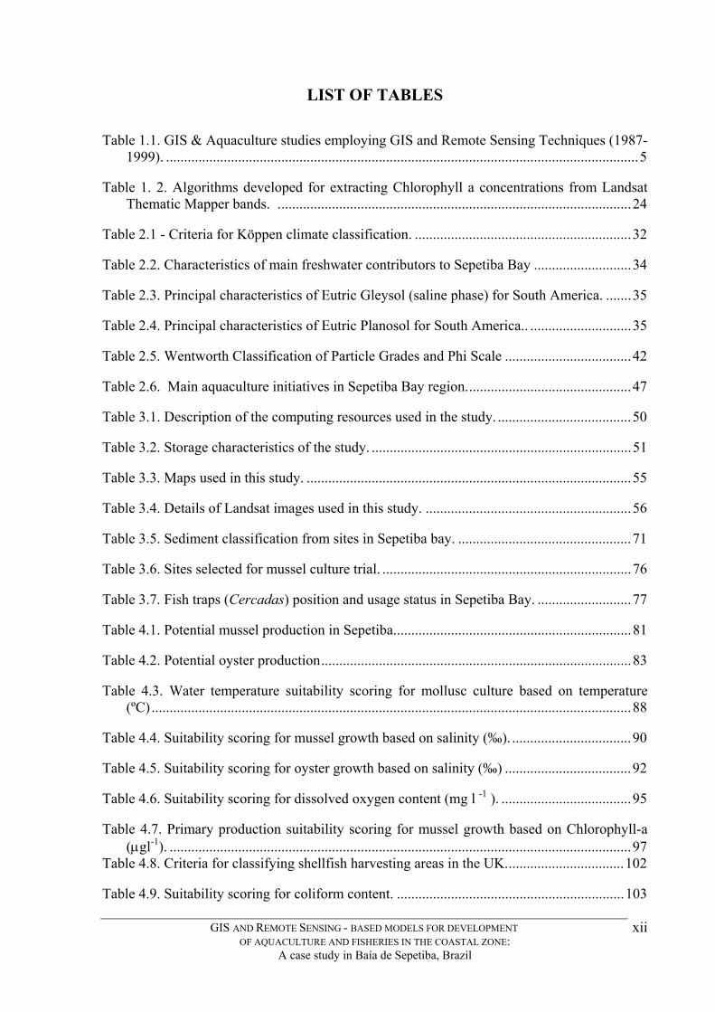
LIST OF TABLES Table 1.1. GIS & Aquaculture studies employing GIS and Remote Sensing Techniques (1987-

1999). ...................................................................................................................................5 Table 1. 2. Algorithms developed for extracting Chlorophyll a concentrations from Landsat

Thematic Mapper bands. ..................................................................................................24 Table 2.1 - Criteria for Köppen climate classification. ............................................................32 Table 2.2. Characteristics of main freshwater contributors to Sepetiba Bay ...........................34 Table 2.3. Principal characteristics of Eutric Gleysol (saline phase) for South America. .......35 Table 2.4. Principal characteristics of Eutric Planosol for South America.. ............................35 Table 2.5. Wentworth Classification of Particle Grades and Phi Scale ...................................42 Table 2.6. Main aquaculture initiatives in Sepetiba Bay region..............................................47 Table 3.1. Description of the computing resources used in the study. .....................................50 Table 3.2. Storage characteristics of the study. ........................................................................51 Table 3.3. Maps used in this study. ..........................................................................................55 Table 3.4. Details of Landsat images used in this study. .........................................................56 Table 3.5. Sediment classification from sites in Sepetiba bay. ................................................71 Table 3.6. Sites selected for mussel culture trial. .....................................................................76 Table 3.7. Fish traps (Cercadas) position and usage status in Sepetiba Bay. ..........................77 Table 4.1. Potential mussel production in Sepetiba..................................................................81 Table 4.2. Potential oyster production......................................................................................83 Table 4.3. Water temperature suitability scoring for mollusc culture based on temperature

(ºC).....................................................................................................................................88 Table 4.4. Suitability scoring for mussel growth based on salinity (‰). .................................90 Table 4.5. Suitability scoring for oyster growth based on salinity (‰) ...................................92 Table 4.6. Suitability scoring for dissolved oxygen content (mg l -1 ). ....................................95 Table 4.7. Primary production suitability scoring for mussel growth based on Chlorophyll-a

(µgl-1). ................................................................................................................................97 Table 4.8. Criteria for classifying shellfish harvesting areas in the UK.................................102 Table 4.9. Suitability scoring for coliform content. ...............................................................103



xii

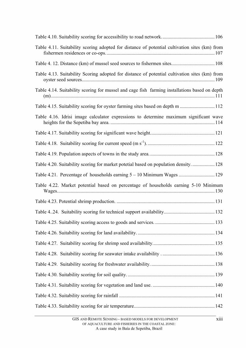
Table 4.10. Suitability scoring for accessibility to road network...........................................106 Table 4.11. Suitability scoring adopted for distance of potential cultivation sites (km) from

fishermen residences or co-ops........................................................................................107 Table 4. 12. Distance (km) of mussel seed sources to fishermen sites...................................108 Table 4.13. Suitability Scoring adopted for distance of potential cultivation sites (km) from

oyster seed sources...........................................................................................................109 Table 4.14. Suitability scoring for mussel and cage fish farming installations based on depth

(m)....................................................................................................................................111 Table 4.15. Suitability scoring for oyster farming sites based on depth m ............................112 Table 4.16. Idrisi image calculator expressions to determine maximum significant wave

heights for the Sepetiba bay area. ....................................................................................114 Table 4.17. Suitability scoring for significant wave height....................................................121 Table 4.18. Suitability scoring for current speed (m s-1). ......................................................122 Table 4.19. Population aspects of towns in the study area. ....................................................128 Table 4.20. Suitability scoring for market potetial based on population density. ..................128 Table 4.21. Percentage of households earning 5 – 10 Minimum Wages .............................129 Table 4.22. Market potential based on percentage of households earning 5-10 Minimum

Wages...............................................................................................................................130 Table 4.23. Potential shrimp production. ...............................................................................131 Table 4..24. Suitability scoring for technical support availability.........................................132 Table 4.25. Suitability scoring access to goods and services. ................................................133 Table 4.26. Suitability scoring for land availability. ..............................................................134 Table 4.27. Suitability scoring for shrimp seed availability..................................................135 Table 4.28. Suitability scoring for seawater intake availability . ..........................................136 Table 4.29. Suitability scoring for freshwater availability. ...................................................138 Table 4.30. Suitability scoring for soil quality. ......................................................................139 Table 4.31. Suitability scoring for vegetation and land use. ..................................................140 Table 4.32. Suitability scoring for rainfall .............................................................................141 Table 4.33. Suitability scoring for air temperature.................................................................142



xiii

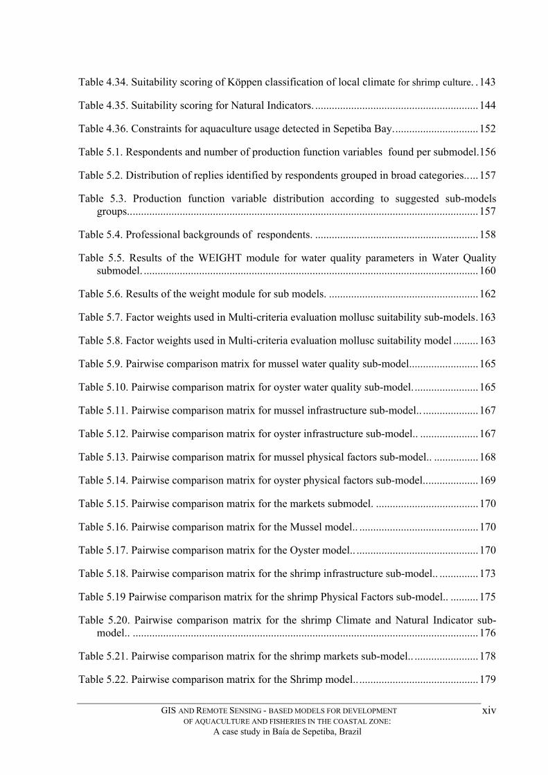
Table 4.34. Suitability scoring of Köppen classification of local climate for shrimp culture. .143 Table 4.35. Suitability scoring for Natural Indicators. ...........................................................144 Table 4.36. Constraints for aquaculture usage detected in Sepetiba Bay...............................152 Table 5.1. Respondents and number of production function variables found per submodel.156 Table 5.2. Distribution of replies identified by respondents grouped in broad categories.....157 Table 5.3. Production function variable distribution according to suggested sub-models

groups...............................................................................................................................157 Table 5.4. Professional backgrounds of respondents. ...........................................................158 Table 5.5. Results of the WEIGHT module for water quality parameters in Water Quality

submodel. .........................................................................................................................160 Table 5.6. Results of the weight module for sub models. ......................................................162 Table 5.7. Factor weights used in Multi-criteria evaluation mollusc suitability sub-models.163 Table 5.8. Factor weights used in Multi-criteria evaluation mollusc suitability model .........163 Table 5.9. Pairwise comparison matrix for mussel water quality sub-model.........................165 Table 5.10. Pairwise comparison matrix for oyster water quality sub-model........................165 Table 5.11. Pairwise comparison matrix for mussel infrastructure sub-model.. ....................167 Table 5.12. Pairwise comparison matrix for oyster infrastructure sub-model.. .....................167 Table 5.13. Pairwise comparison matrix for mussel physical factors sub-model.. ................168 Table 5.14. Pairwise comparison matrix for oyster physical factors sub-model....................169 Table 5.15. Pairwise comparison matrix for the markets submodel. .....................................170 Table 5.16. Pairwise comparison matrix for the Mussel model.. ...........................................170 Table 5.17. Pairwise comparison matrix for the Oyster model.. ............................................170 Table 5.18. Pairwise comparison matrix for the shrimp infrastructure sub-model.. ..............173 Table 5.19 Pairwise comparison matrix for the shrimp Physical Factors sub-model.. ..........175 Table 5.20. Pairwise comparison matrix for the shrimp Climate and Natural Indicator sub-

model.. .............................................................................................................................176 Table 5.21. Pairwise comparison matrix for the shrimp markets sub-model.. .......................178 Table 5.22. Pairwise comparison matrix for the Shrimp model.. ...........................................179



xiv

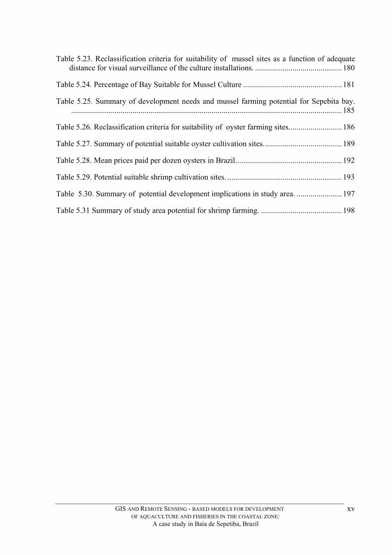
Table 5.23. Reclassification criteria for suitability of mussel sites as a function of adequate

distance for visual surveillance of the culture installations. ............................................180 Table 5.24. Percentage of Bay Suitable for Mussel Culture ..................................................181 Table 5.25. Summary of development needs and mussel farming potential for Sepebita bay.

.........................................................................................................................................185 Table 5.26. Reclassification criteria for suitability of oyster farming sites...........................186 Table 5.27. Summary of potential suitable oyster cultivation sites........................................189 Table 5.28. Mean prices paid per dozen oysters in Brazil......................................................192 Table 5.29. Potential suitable shrimp cultivation sites. ..........................................................193 Table 5.30. Summary of potential development implications in study area. .......................197 Table 5.31 Summary of study area potential for shrimp farming. .........................................198



xv

CHAPTER 1.

GENERAL INTRODUCTION

1.1 - Introduction

By the late 1990s, the western region of Rio de Janeiro, which includes Sepetiba Bay (Baía de

Sepetiba) was beginning to experience the socio-economic and ecological consequences of

urban sprawl and industrial pollution. Most of the changes had occurred during the 1970s.

The fact that mangroves in Brazil are protected by law, and that fishermen in the study area

generally respect the shallow waters which are important for the initial phases of shrimp

development, has not been sufficient to guarantee the livelihood of those dependent on coastal

natural resources such as fisheries. The number of people exploiting professionally,

artisanally or for recreational purposes, the various stocks of fish and shellfish available in the

study area, has increased over the years. For better overall natural resources management,

there is a need for a good understanding of the actors in the area and their impacts. This is

urgent and requires the kind of spatially comprehensive analysis that is now possible.

Due to its special maritime

connections and strategic location

on the 7,364 km Brazilian

coastline, Rio de Janeiro state is a

priority (Fig 1.1). The state has an

636 km coastline where 80% of its

ca. 13 million inhabitants compete

for living and working space

amidst mangroves, coastal

lagoons, coastal marshes, beaches

and islands. Among this

population are the artisanal

fishermen.

Fig. 1.1. Regional position of the State of Rio de Janeiro, Brazil.



1

Fishing in nearshore coastal waters and shallow shelf areas constitutes over 90% of the

employment possibilities in fisheries and is an essential and conservative component of

coastal communities. Estuarine and lagoon resources, in particular, have a major socio-

economic importance in fisheries (Caddy and Griffiths, 1995).

Coastal waters have always provided access to marine living resources which are important

both as a source of food and for leisure purposes. With human population growth occurring

preferentially along coastlines, these waters have not only become valuable as leisure sites but

also as ultimate discharge sites for several polluting activities. This is clearly the case for

Brazil where currently the coastal population density is 87/km2 which is 5 times that of the

national average, 17/km2 (Ministério do Meio Ambiente, 1999). This trend of expansion and

utilisation of natural resources highlights the urgent need to develop and implement an

Integrated Coastal Zone Management (ICZM) scheme.

An (ICZM) is “a planning and co-ordinating process which deals with development

management and coastal resources and which is focused on the land water interface”. (Clark,

1992). The driving forces for ICZM include the high rate of population growth, poverty,

dwindling natural resources, large-scale, quick-profit commercial enterprises which degrade

resources, lack of awareness about management for resource sustainability among local

people, lack of understanding of the economic contribution of coastal resources to society and

lack of serious government follow-up and support for conservation programmes. All of these

can be identified in the study area. The overall goal of Integrated Coastal Management (ICM)

is “to improve the quality of life of human communities who depend on coastal resources

while maintaining the biological diversity and productivity of coastal ecosystems” (GESAMP,

1996).

In Brazil, the government began its coastal management policy, constituted by law in 1988,

which later became the Plano Nacional de Gerenciamento Costeiro (PNGC). This was revised

recently in 1997 to become the PNGC II. At the present time, the state department responsible

for guiding the elaboration of the coastal management plan for the state of Rio de Janeiro,

Fundação Estadual de Engenharia do Meio Ambiente (FEEMA), is still developing this plan,

and so official information is unavailable (FEEMA, 1999).



2

One of the key issues in managing the environment is ‘sustainability’. Sneadaker and Getter

(1985) defined sustainable resources use as “the resource not be harvested, extracted or

utilised in excess of the amount which can be regenerated. In essence, the resource is seen as a

capital investment with an annual yield; it is, therefore, the yield that is utilised and not the

capital investment which is the resource base. By sustaining the resource base, annual yields

are assured in perpetuity”

Because aquaculture and fisheries production in coastal zones are such important food sources

and revenue generating activities to coastal populations, planned and Integrated Coastal Zone

Management (ICZM) has an important role in promoting sustainability of natural coastal

resources.

Barg (1992) reviewed the socio-economic benefits arising from aquaculture activity which

includes the provision of food, contributing to improved nutrition and health, generation of

income and employment and also in part to compensate for the low growth rate of capture

fisheries. Sustainable development of aquaculture can contribute to the prevention and control

of aquatic pollution since it relies essentially on good water quality resources. It is in the

interest of growers to select good water quality and productive areas, and maintain unpolluted

conditions. Furthermore, culture of molluscs can in certain cases counteract the process of

nutrient enrichment in eutrophic waters. This is one of the assumptions maintained by the

Swedish government in their Sustainable Coastal Zone Management of Marine Resources

programme (SUCOZOMA) where mussel farms will be tested for their potential to reduce

nutrient levels in coastal waters (SUCOZOMA, 1999). Haamer (1996) designed a model

showing that if mussel farms were developed to cover from 1% to 2.4% of fjord surface

waters around the Orust and Tjörn islands in Sweden, the Dissolved Inorganic Nitrogen (DIN)

level could be reduced by 20%, effectively the same as in the cleaner, more open waters of the

Skageraak.



3

1.2 - Geographical Information Systems

UNITAR (1995) described Geographic Information Systems (GIS) as being “as significant to

spatial analysis as the inventions of the microscope and telescope were to science” and that

they represent “the biggest step forward in the handling of geographic information since the

map” GIS systems have evolved, and been commercially developed by a number of

companies, into sophisticated and sometimes expensive packages. GIS has found its use in

several sectors of modern society from municipal planning, sales, marketing and

infrastructural planning to precision farming.

There are several definitions for GIS. According to Burrough & McDonnell (1998), these can

be toolbox based, database or organisation-based. For the purposes of this study, the database

definition which states that GIS is “a database system in which most of the data are spatially

indexed, and upon which a set of procedures operate in order to answer queries about spatial

entities in the database” does not suffice, since several queries will be made to, and based on,

manipulations and extrapolations to the database and which go well beyond simple database

query. The ‘toolbox-based’ definition complements the previous one and is much more

appropriate as it defines GIS as “a system for capturing, storing, checking, manipulating,

analysing and displaying data which are spatially referenced to the earth” (DeMers, 1997). It

is the analysis subsystem, which is the heart of the GIS and it is this aspect that differentiates

several competing GIS softwares.

Knox and Smith (1997) reviewed early major implementations of GIS and found that in one

of its earliest examples, the Canadian government designed a GIS to manage forestry and

other types of land use. The academic sector took an interest in GIS potential in its earliest

stages and had a large role in its development. Harvard University created its own GIS, called

SYMAP (Knox and Smith, 1997). From the academic sector stemmed commercial companies

such as Environmental Systems Research Institute (ESRI) which was initially created as a

non-profit organisation and Intergraph, a well known supplier to the GIS market. These have

grown and developed successful applications packages such as ARC/INFO, launched in 1982,

one of the most widely used in the world. Some systems were aimed basically at teaching.

One such system was OSU-MAP for the PC developed by Ohio State University, which was

originally a single disk GIS installation.



4

Another similar system was IDRISI developed at Clark Labs, an educational and research

institution located at Clark University in Worcester, Massachusetts, USA. The organisation,

founded in 1987, (Eastman, R.J. 1997) has developed training materials in the form of tutorial

exercises and data that guide the new user through the concepts of GIS and Image Processing.

Because of its low cost and advanced capabilities, IDRISI has been a popular choice for

teaching GIS and Image Processing at the university level. Clark Labs has developed for

UNITAR (United Nations Institute for Training and Research) a training program with a set

of exercises using real-world data to explore environmental issues (IDRISI, 2002). It has a

very large academic user base.

1.3 - GIS use in Aquaculture and Fisheries

A search of the ‘Aquatic Sciences and Fisheries Abstracts’ (ASFA) database using the

keywords “aquaculture and GIS” retrieves only 83 titles for the period 1978-2002. Although

the ASFA database is fairly comprehensive, it does not cover all studies in the so-called ‘grey

literature’, some of which have been identified and are referred to in the course of this study.

Even including such references, the fact remains that despite the usefulness of GIS as an

aquaculture-assisting tool it is still far from being widely adopted in the sector. However,

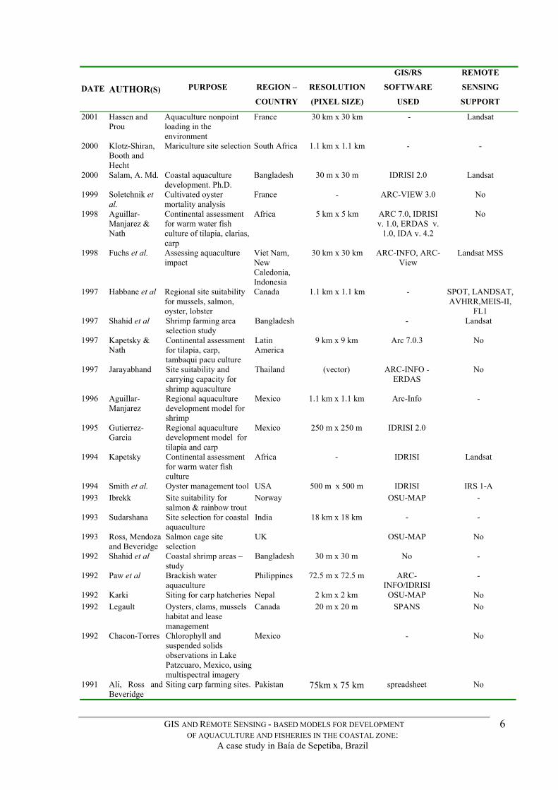
some progress has been made and Table 1.1 summarizes the most pertinent applications of

GIS and Remote Sensing for aquaculture and fisheries.

Table 1.1. GIS & Aquaculture studies employing GIS and Remote Sensing Techniques (1987-1999). DATE

AUTHOR(S)

PURPOSE

REGION –

COUNTRY

RESOLUTION

(PIXEL SIZE)

GIS/RS

SOFTWARE

USED

REMOTE

SENSING

SUPPORT

2002 Scott, Vianna and Mathias

Aquaculture Potential Study for Rio de Janeiro

Brazil 30 m x 30 m Spring 3.5, ARC-VIEW 3.2

LANDSAT

2002 Geitner Cage trout in marine environment

Denmark 100 m x 100 m ARC-VIEW 3.2, ARC-VIEW GIS

8.2

No

2002 Perez, Telfer and Ross

Mariculture site selection Spain 1.1 km x 1.1 km IDRISI 2.0 AVHRR

2002 Bonetti, Beltrame and Bonetti

Shrimp culture, hydrological suitability index

Brazil - ARC-VIEW 3.2/ Surfer

-

2002 Barroso and Bonetti

Shellfish planning study Brazil 4 m x 4 m IDRISI 32 Aerial photos



5

DATE

AUTHOR(S)

PURPOSE

REGION –

COUNTRY

RESOLUTION

(PIXEL SIZE)

GIS/RS

SOFTWARE

USED

REMOTE

SENSING

SUPPORT

2001 Hassen and Prou

Aquaculture nonpoint loading in the environment

France 30 km x 30 km - Landsat

2000 Klotz-Shiran, Booth and Hecht

Mariculture site selection South Africa 1.1 km x 1.1 km - -

2000 Salam, A. Md. Coastal aquaculture development. Ph.D.

Bangladesh 30 m x 30 m IDRISI 2.0 Landsat

1999 Soletchnik et al.

Cultivated oyster mortality analysis

France - ARC-VIEW 3.0 No

1998 Aguillar-Manjarez & Nath

Continental assessment for warm water fish culture of tilapia, clarias, carp

Africa 5 km x 5 km ARC 7.0, IDRISI v. 1.0, ERDAS v.

1.0, IDA v. 4.2

No

1998 Fuchs et al. Assessing aquaculture impact

Viet Nam, New Caledonia, Indonesia

30 km x 30 km ARC-INFO, ARC-View

Landsat MSS

1997 Habbane et al Regional site suitability for mussels, salmon, oyster, lobster

Canada 1.1 km x 1.1 km - SPOT, LANDSAT, AVHRR,MEIS-II,

FL1 1997 Shahid et al Shrimp farming area

selection study Bangladesh

- Landsat

1997 Kapetsky & Nath

Continental assessment for tilapia, carp, tambaqui pacu culture

Latin America

9 km x 9 km Arc 7.0.3 No

1997 Jarayabhand Site suitability and carrying capacity for shrimp aquaculture

Thailand (vector) ARC-INFO - ERDAS

No

1996 Aguillar-Manjarez

Regional aquaculture development model for shrimp

Mexico 1.1 km x 1.1 km Arc-Info -

1995 Gutierrez-Garcia

Regional aquaculture development model for tilapia and carp

Mexico 250 m x 250 m IDRISI 2.0

1994 Kapetsky Continental assessment for warm water fish culture

Africa - IDRISI Landsat

1994 Smith et al. Oyster management tool USA 500 m x 500 m IDRISI IRS 1-A 1993 Ibrekk Site suitability for

salmon & rainbow trout Norway

OSU-MAP -

1993 Sudarshana Site selection for coastal aquaculture

India 18 km x 18 km - -

1993 Ross, Mendoza and Beveridge

Salmon cage site selection

UK

OSU-MAP No

1992 Shahid et al Coastal shrimp areas – study

Bangladesh 30 m x 30 m No -

1992 Paw et al Brackish water aquaculture

Philippines 72.5 m x 72.5 m ARC-INFO/IDRISI

-

1992 Karki Siting for carp hatcheries Nepal 2 km x 2 km OSU-MAP No 1992 Legault Oysters, clams, mussels

habitat and lease management

Canada 20 m x 20 m SPANS No

1992 Chacon-Torres Chlorophyll and suspended solids observations in Lake Patzcuaro, Mexico, using multispectral imagery

Mexico - No

1991 Ali, Ross and Beveridge

Siting carp farming sites. Pakistan 75km x 75 km spreadsheet No



6

DATE

AUTHOR(S)

PURPOSE

REGION –

COUNTRY

RESOLUTION

(PIXEL SIZE)

GIS/RS

SOFTWARE

USED

REMOTE

SENSING

SUPPORT

1990 Flores-Nava Regional warm freshwater fish farming potential

Mexico 1.2 km x 0.816 km OSU-MAP for the PC

-

1990 Kapetsky et al Regional catfish and crawfish farming assessment

USA - ELAS -

1990 Kapetsky et al Assessing country potential for tilapia & catfish

Ghana 2 km x 2 km IDRISI No

1990 Krieger & Muslow

Salmonid and mussel farm siting

Chile - ROOTS 4.0, GRASS 3.0

No

1989 Kapetsky Regional suitability assessment shrimp and fish

Malaysia - ERDAS 7.2 SPOT

1989 Pheng Coastal resources management

Malaysia SPANS SPOT- Landsat

1988 Kapetsky, Hill and Worthy

Catfish farming siting USA

ELAS no

1987 Meaden Trout farming siting UK 10km x 10 km spreadsheet no 1987 Kapetsky Aquaculture

development Zimbabwe 30 m x 30 m No Landsat

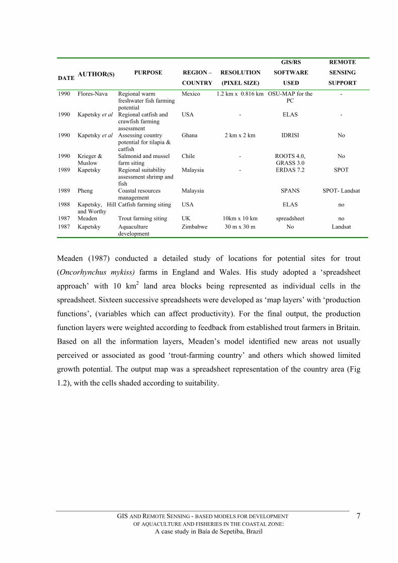
Meaden (1987) conducted a detailed study of locations for potential sites for trout

(Oncorhynchus mykiss) farms in England and Wales. His study adopted a ‘spreadsheet

approach’ with 10 km2 land area blocks being represented as individual cells in the

spreadsheet. Sixteen successive spreadsheets were developed as ‘map layers’ with ‘production

functions’, (variables which can affect productivity). For the final output, the production

function layers were weighted according to feedback from established trout farmers in Britain.

Based on all the information layers, Meaden’s model identified new areas not usually

perceived or associated as good ‘trout-farming country’ and others which showed limited

growth potential. The output map was a spreadsheet representation of the country area (Fig

1.2), with the cells shaded according to suitability.



7

Fig 1.2. Schematic representation of spreadsheet use in aquaculture GIS.

Although the study did not use a ‘package GIS’, the principle used was the same. Pauly et al

(1997), developed a software (B:RUN) based on LOTUS 1-2-3 spreadsheet for data entry and

production of low-level geographic information system, available free of any copyright

restrictions. It has been used by the authors to simulate stock dynamics of demersal fish and

fleet operations in the coastal waters of Brunei Darussalam.

One of the pioneering applications of GIS for aquaculture is that of Kapetsky, McGregor &

Nanne (1987), who implemented a GIS study for the Gulf of Nicoya, Costa Rica, in order to

assist in finding the most promising locations and their areal extent for various aquaculture

development opportunities. It was also one of the early attempts at integrating a satellite

image into an aquaculture GIS. Three kinds of aquaculture development opportunities were

evaluated in terms of optimum locations and land and water surface areas available: (1)

culture of molluscs in intertidal and subtidal areas as well as suspended culture of molluscs

and cage culture of fish, (2) extensive culture of shrimp and fish in existing solar salt ponds,

and (3) semi-intensive shrimp farming along the gulf shoreline outside mangrove areas. The

study approach used was later included by the United Nations Institute for Training and

Research as a GIS training exercise in “Applications in Coastal Zone Research and

Management” (UNITAR, 1995).

Catfish (Ictalurus punctatus) aquaculture in the U.S. has been an important part of the

aquaculture industry for the last 30 years.



8

It was in the context of developing this frontier that another early application of GIS in

aquaculture was undertaken by Kapetsky, Hill and Worthy (1988). A GIS was implemented to

identify and inventory areas which were physiographically suitable for further catfish

farming, based on soil characteristics and susceptibility to flooding, in Franklin Parish,

Louisiana, USA. The region had, at the time, over 1,000 ha of farms producing nearly 1,000

tons of catfish from 40 different sites. A good correspondence was obtained between the

locations of existing catfish farms and suitable locations determined by the GIS. This

potential use of GIS for assisting the location of new sites was very encouraging.

The need for good analysis tools, capable of handling the many distinct components of an

aquaculture information database, including climate, water quantity and quality, soil types,

markets, infra-structure and other general information for integration through specific

mathematical operations for output, followed parallel to GIS software development. Ali, Ross

and Beveridge (1991) developed a simple GIS system intended for analysing best

opportunities for extensive carp farming in Pakistan using an electronic spreadsheet (View

Sheet). Several sheets were made containing information on the available parameters and

simple mathematical models produced a final spreadsheet with a grey-scale visual

representation of Pakistani carp farming potential. By attributing values to cells in a

spreadsheet, this study also effectively used the same tesseral technique, or ‘grid’ concept, of

raster-based GIS software.

With the expansion of shrimp farming in the 1980s, several countries transformed mangrove

areas into shrimp growing ponds. Malaysia had set a target for opening and developing

21,000 ha of shrimp ponds for the year 2000. It was in this context that FAO technical

assistance conducted a training programme for the fisheries personnel on GIS technology

(Kapetsky, 1989). Similar to the Gulf of Nicoya study, the objective of the aquaculture

development GIS for Johor State, Malaysia, was to locate and quantify opportunities for

further aquaculture development, targeted at shrimp (Penaeus monodon) farming in ponds

and fish culture in cages. Locational criteria and rating systems were established by

considering species physiology and culture technologies available at the time, in relation to

the local environment and infrastructures.



9

This study was rich in the methodology it employed and was also practical, for it was able to

verify, in the field, the predicted outcomes achieved by modelling, with several operating

shrimp farms existing in the study area.

OSU-MAP for the PC 3.0 was used creatively by Ross, Mendoza and Beveridge (1993) in

coastal aquaculture site selection for salmon (Salmo salar) cage-culture development in

Camas Bruaich Ruaidhe, Oban, Argyll, Scotland. This study accomplished the site selection

by processing several information layers, such as basic water quality needs of salmonid

farming, and limitations, such as current velocities and exposure to inadequate wave heights

predicted from a bathymetry/wind fetch/wind velocity relationship. Flores-Nava (1990) also

used OSU-MAP to identify potential inland areas for aquaculture development of mojarra

(Cichlasoma urophthalmus) and tilapia (Oreochromis niloticus) in the Yucatán Peninsula.

This is one of the earliest references which takes into account socio-economic components in

an aquaculture GIS study. Flores-Nava modelled the market demand and social environment

through the creation of layers indicating availability and proximity of distribution centres and

extension services. Another innovative aspect of this study was a sub-model which described

the level of intensification that reservoirs could withstand.

In investigating site suitability for aquaculture, GIS can incorporate many layers and a wide

range of factors. Krieger and Muslow (1990) contributed to GIS-assisted site suitability

studies by incorporating a ‘biological indicator’ layer for siting fish farming and mussel

culture in the subtidal regions of Yaldad Bay, southern Chile. In addition to the traditional

map layers describing the physical environment, such as bathymetry, salinity, sediment types,

organic content, etc., the authors included ‘percentage of shells in the sediment’, ‘number of

species’ and ‘density of macroinfauna’ as supporting map layers used in their modelling

scheme (see Fig 1.3). This step improved the potential use of the GIS from a technically

straightforward site selection assisting tool, which took into account traditional abiotic factors

expressed as thematic layers, to one which was a more sophisticated modelling tool with

potential for marine benthic resource management.



10

Fig 1.3. Benthic mussel site suitablility model for Yaldad Bay, Chile. Adapted from Krieger and Muslow, 1990.

GIS has been used for some applications in coastal management. A good example is that

developed by Legault (1992), who employed a GIS for the Eastern Prince Edward Island,

Canada, to determine areas for shellfish growing leases, shellfish harvesting zones and

contaminated closure zones. A comparison was made between these areas and an estimated

cash value was determined. Further uses of the GIS were briefly explored, in particular, its

usefulness as a planning tool to avoid pollution sources and to assist in prioritizing research

surveys. A similar application has been developed for the mollusc bivalve mudflats of

Algarve, Portugal using ARC-View (João Cuña, unpublished, 1998). Other benthic resource

researchers have been interested in the capabilities of GIS. Smith, Jordan and Greenhawk

(1994) developed a desk-top GIS-based management information system with the intention of

managing Maryland's Chesapeake Bay oyster populations. GIS-assisted coastal shellfish

aquaculture potential was also estimated by Cansado-Marrero (1998) who used GIS to make

preliminary models of mussel (Perna perna) and oyster (Crassostrea rhizophorae) production

potential in a sub-tropical coastal semi-enclosed lagoon, Baía de Sepetiba, Brazil.



11

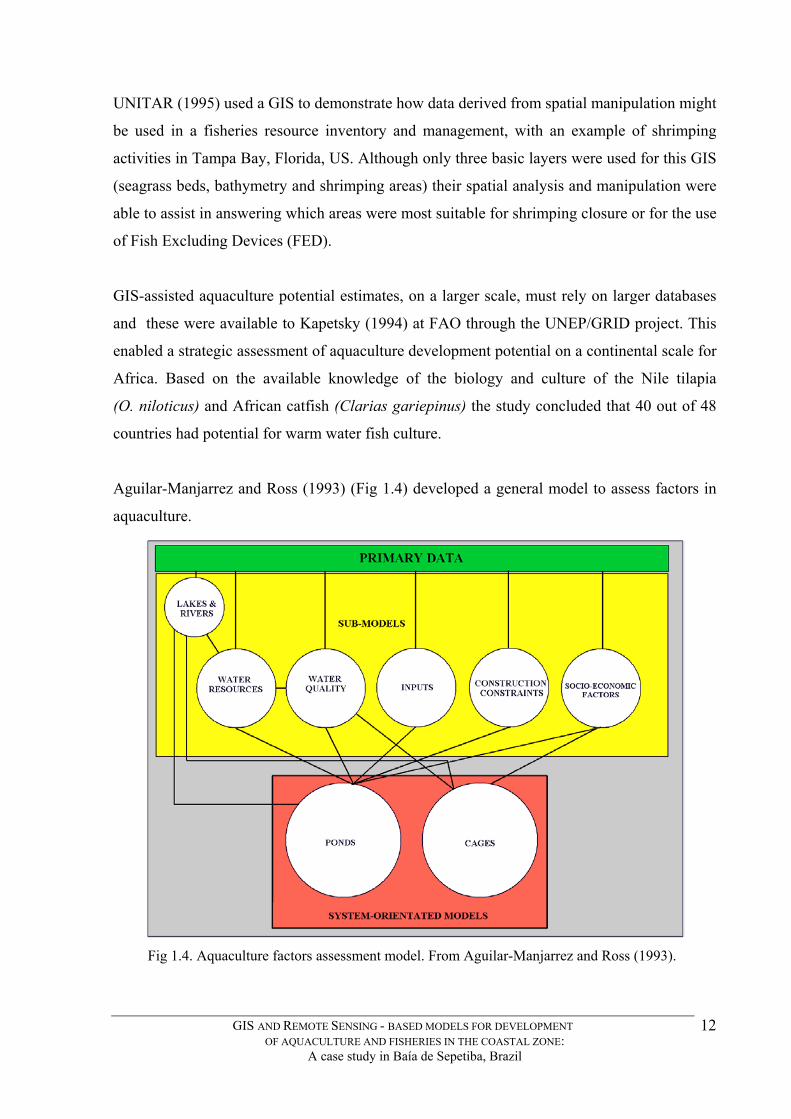
UNITAR (1995) used a GIS to demonstrate how data derived from spatial manipulation might

be used in a fisheries resource inventory and management, with an example of shrimping

activities in Tampa Bay, Florida, US. Although only three basic layers were used for this GIS

(seagrass beds, bathymetry and shrimping areas) their spatial analysis and manipulation were

able to assist in answering which areas were most suitable for shrimping closure or for the use

of Fish Excluding Devices (FED).

GIS-assisted aquaculture potential estimates, on a larger scale, must rely on larger databases

and these were available to Kapetsky (1994) at FAO through the UNEP/GRID project. This

enabled a strategic assessment of aquaculture development potential on a continental scale for

Africa. Based on the available knowledge of the biology and culture of the Nile tilapia

(O. niloticus) and African catfish (Clarias gariepinus) the study concluded that 40 out of 48

countries had potential for warm water fish culture.

Aguilar-Manjarrez and Ross (1993) (Fig 1.4) developed a general model to assess factors in

aquaculture.

Fig 1.4. Aquaculture factors assessment model. From Aguilar-Manjarrez and Ross (1993).



12

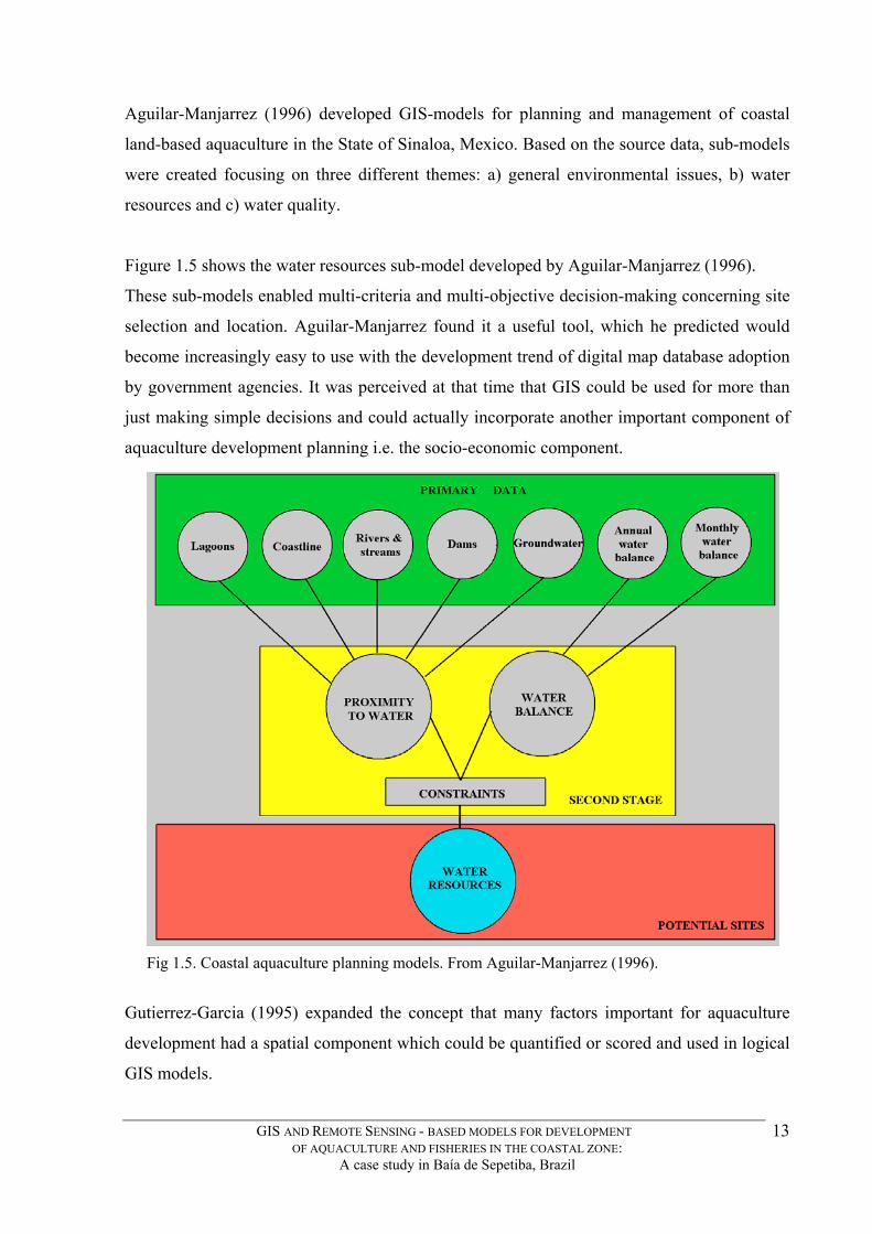
Aguilar-Manjarrez (1996) developed GIS-models for planning and management of coastal

land-based aquaculture in the State of Sinaloa, Mexico. Based on the source data, sub-models

were created focusing on three different themes: a) general environmental issues, b) water

resources and c) water quality.

Figure 1.5 shows the water resources sub-model developed by Aguilar-Manjarrez (1996).

These sub-models enabled multi-criteria and multi-objective decision-making concerning site

selection and location. Aguilar-Manjarrez found it a useful tool, which he predicted would

become increasingly easy to use with the development trend of digital map database adoption

by government agencies. It was perceived at that time that GIS could be used for more than

just making simple decisions and could actually incorporate another important component of

aquaculture development planning i.e. the socio-economic component.

Fig 1.5. Coastal aquaculture planning models. From Aguilar-Manjarrez (1996).

Gutierrez-Garcia (1995) expanded the concept that many factors important for aquaculture

development had a spatial component which could be quantified or scored and used in logical

GIS models.



13

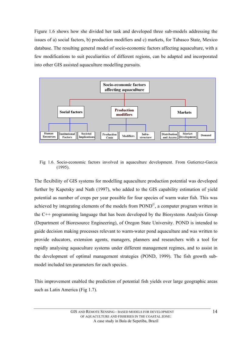
Figure 1.6 shows how she divided her task and developed three sub-models addressing the

issues of a) social factors, b) production modifiers and c) markets, for Tabasco State, Mexico

database. The resulting general model of socio-economic factors affecting aquaculture, with a

few modifications to suit peculiarities of different regions, can be adapted and incorporated

into other GIS assisted aquaculture modelling pursuits.

Fig 1.6. Socio-economic factors involved in aquaculture development. From Gutierrez-Garcia

(1995).

The flexibility of GIS systems for modelling aquaculture production potential was developed

further by Kapetsky and Nath (1997), who added to the GIS capability estimation of yield

potential as number of crops per year possible for four species of warm water fish. This was

achieved by integrating elements of the models from POND©, a computer program written in

the C++ programming language that has been developed by the Biosystems Analysis Group

(Department of Bioresource Engineering), of Oregon State University. POND is intended to

guide decision making processes relevant to warm-water pond aquaculture and was written to

provide educators, extension agents, managers, planners and researchers with a tool for

rapidly analysing aquaculture systems under different management regimes, and to assist in

the development of optimal management strategies (POND, 1999). The fish growth sub-

model included ten parameters for each species.

This improvement enabled the prediction of potential fish yields over large geographic areas

such as Latin America (Fig 1.7).



14

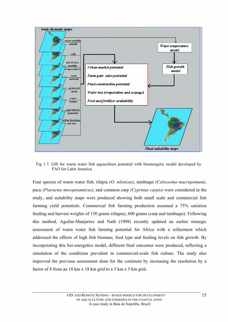
Fig 1.7. GIS for warm water fish aquaculture potential with bioenergetic model developed by FAO for Latin America.

Four species of warm water fish: tilápia (O. niloticus), tambaqui (Colossoma macropomum),

pacu (Piaractus mesopotamicus), and common carp (Cyprinus carpio) were considered in the

study, and suitability maps were produced showing both small scale and commercial fish

farming yield potentials. Commercial fish farming production assumed a 75% satiation

feeding and harvest weights of 150 grams (tilapia), 600 grams (carp and tambaqui). Following

this method, Aguilar-Manjarrez and Nath (1998) recently updated an earlier strategic

assessment of warm water fish farming potential for Africa with a refinement which

addressed the effects of high fish biomass, feed type and feeding levels on fish growth. By

incorporating this bio-energetics model, different final outcomes were produced, reflecting a

simulation of the conditions prevalent in commercial-scale fish culture. The study also

improved the previous assessment done for the continent by increasing the resolution by a

factor of 4 from an 18 km x 18 km grid to a 5 km x 5 km grid.



15

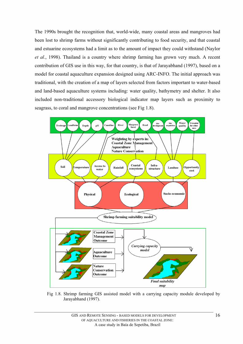
The 1990s brought the recognition that, world-wide, many coastal areas and mangroves had

been lost to shrimp farms without significantly contributing to food security, and that coastal

and estuarine ecosystems had a limit as to the amount of impact they could withstand (Naylor

et al., 1998). Thailand is a country where shrimp farming has grown very much. A recent

contribution of GIS use in this way, for that country, is that of Jarayabhand (1997), based on a

model for coastal aquaculture expansion designed using ARC-INFO. The initial approach was

traditional, with the creation of a map of layers selected from factors important to water-based

and land-based aquaculture systems including: water quality, bathymetry and shelter. It also

included non-traditional accessory biological indicator map layers such as proximity to

seagrass, to coral and mangrove concentrations (see Fig 1.8).

Fig 1.8. Shrimp farming GIS assisted model with a carrying capacity module developed by Jarayabhand (1997).



16

Jarayabhand attempted to balance weights for the selection of aquaculture site development

models by developing preferences based on consultation with experts in the contrasting fields

of (i) Conservation (ii) Coastal Zone Management and (iii) Aquaculture and Fisheries

Development. Jarayabhand’s greater contribution was the development of a carrying capacity

sub-model for shrimp aquaculture, another input for the decision making process, which

allowed determination of a cut-off point for the upper limit allocatable to aquaculture

development, so as not to exceed the carrying capacity for Nitrogen and Phosphorus loads to

the local environment.The methodology used to establish these weights was the Analytical

Hierarchy Process (AHP) developed by Saaty (1995). Aguilar-Manjarez (1996) also used this

process which establishes weights and exists as a well developed Multi-Criteria Evaluation

module within the IDRISI GIS. Perez-Martinez, (2002) used GIS-based models for

optimisation of marine cage aquaculture in open oceanic waters. Perez-Sanchez, (2002) did a

socio-economic assessment of small-scale aquaculture stakeholders. Salam, (2000) developed

a GIS model for coastal aquaculture development in the Sunderbans, Bangladesh.

Further application and development of GIS in aquaculture siting, planning and development

is clearly possible. So far it has mostly remained within the realms of identifying suitable sites

for implementation, or extending suitable sites considering a series of production variables. In

contrast to aquaculture, the benefits of GIS and RS use in terrestrial farming has led to

precision farming, where feedback to farmers from GIS-RS experts, monitoring specific crops

at specific locations guide them in caring for the best health of the crops by indicating, in

space and with time, areas where appropriate actions need to be made, such as the addition

of fertilizers, pesticides or water. This process already exists and is evolving in terms of new

and higher resolution sensors being launched by commercial ventures (Dudka,1997). The

same type of feedback may be much more difficult to accomplish in water-based aquaculture

systems which suffer in comparison to land-based operations in that there is less room to

make mistakes in choice of site. For example, much of aquaculture depends on the physico-

chemical conditions such as temperature, salinity, oxygen, currents, pollution, algal blooms,

water exchange which dictate whether or not an aquatic species to be cultured can thrive in an

environment (Beveridge, 1996).

GIS is still used in most sectors substantially as a simple cadastral database combining

cadastral date and often factors aimed at simple database query and thematic map output

capabilities. However, it is being used increasingly at the regional planning level.



17

A good example is Sepetiba Bay basin, where a macrozoning process, taking into

consideration ecological and economic factors influencing land uses within the watershed, be

they urban, industrial, agricultural, touristic or nature conservation, etc., is being elaborated

(SEMA, 1996).

Opportunities such as this lead us to suggest that GIS, being a spatial analysis tool, can also be

employed to incorporate within its modelling capabilities the ‘ecological footprint’ concept in

accounting for ecological resources. The ecological footprint is an accounting tool for

ecological resources. (Wackernagel and Rees, 1999). Categories of human consumption, are

translated into areas of productive land (area) required to provide resources and assimilate

waste products. The ecological footprint is a measure of life-style sustainability. This concept

can also be applied to aquaculture in terms of ‘productive water surface’. The ecological

footprint for salmon, shrimp and tilapia aquaculture has been demonstrated by Kautsky et al

(1997), and Naylor et al (1998) who calculated that the ecological footprint for a semi-

intensive shrimp farm in Colombia needs a spatial ecosystem support 35-190 times the

surface of the shrimp pond area (in the mangrove area).

1.4 - Remote Sensing for Aquaculture and Fisheries

The trend to use remotely sensed images to study and assist in selecting potentially suitable

areas for aquaculture development integrated in a GIS is on the increase, as can be seen from

a number of investigations summarised in Table 1. Green et al. (1996) reviewed remote

sensing use for assessing and managing tropical coastal resources including aquaculture such

as shrimp farming and cage siting but also other closely related topics such as seagrass,

mangroves, algae, coral reefs and primary productivity measurements. Remotely sensed

images, such as those obtained from the Landsat and SPOT platforms, are generated and

furnished in a raster format. This format is highly compatible with raster-based GIS software,

facilitating integration and consequent processes of image classification. This compatibility

assists in generating new thematic layers which can incorporated into the GIS database,

increasing the power of the decision making process.

Because of their characteristic reflectance, water bodies are especially visible from several

remote sensing platforms. Kapetsky (1987) took advantage of Landsat’s bands 1, 3 and 4 to

isolate water bodies from vegetation.



18

His study was able to locate 906 water bodies with a surface area between 21,000 and 45,000

ha over 32,400 km2 of territory in Zimbabwe. From this area it was estimated that 7,000 tons

of fish could be produced, thus demonstrating the usefulness of satellite RS for locating and

counting small water bodies for potential fishery and aquaculture development.

The importance of using reflectance at different wavelengths in the coastal areas has been

particularly useful in mangrove areas. Thus CNES-IFREMER (1987) used a SPOT RS image

and GIS for identifying favourable tropical shrimp farming sites in New Caledonia. The study

mostly employed SPOT’s red/infrared capacity to clearly identify different vegetation types

along the coastline as mangroves and associated mudflats. Shahid et al. (1992) also used this

strategy associating infrared colour aerial photographs, Landsat MSS and Landsat TM images

from two different dates, to study coastal shrimp farming areas in Bangladesh. The

investigation clearly showed that more mangrove areas were being cut down in the

Sunderbans and were being replaced with shrimp growing ponds.

Using remotely sensed images to locate appropriate aquaculture sites can be approached in

more than one way. Sudarshana et al. (1993) used data from the IRS 1-A to select sites for

‘coastal aquaculture’ on the West Coast of India in the estuaries of the Kali and Aghanashimi.

Principal emphasis was placed on selecting low lying areas, creeks, marshes, mud flats and

mangroves, for the field study and selecting those most appropriate for aquaculture

development. However, no mention was made of which species would be considered.

Although the study did not use a proper GIS for any analytical work, it did apply a Weighted

Index Scheme (WIS) which was based on inputs from the in situ observations collected at the

time of the satellite overpass. The study failed to provide a clear picture of potential

aquaculture sites as a function of the broader range of aquaculture variables. However, the

methodology developed is rather interesting because it used an indicator for aquaculture

selection based on ‘bioturbation’ from satellite imagery analysis. This indicator was

developed as a composite result of the analysis of four parameters: a) benthic biomass against

band 1, b) phaeopigment quality in water against band 2, c) sediment particle size against

band 3 and d) concentration of humic substances in the sediment against band 4. As these

factors are found to influence the spectral radiance over water in estuarine areas the

‘bioturbation indicator’ as indicated by remotely sensed images could become a useful tool in

other ecological studies.



19

However, bioturbation is a phenomenon caused by burrowing activities of many organisms

ranging from marine annelids to terrestrial anteaters. It would be necessary to know which

group is responsible for the bioturbation observed, as some bioturbators may be highly

resistant to pollution, and, therefore, this index is not necessarily a good indicator of

suitability for aquaculture.

Water temperature is probably the most important factor in determining aquaculture

production potential. Grenier et al (1989) used Landsat TM and NOAA-AVHRR images to

extract surface water temperature for detecting potential aquaculture sites in Canada. In a

further step of this study carried out by Habbane, El-Sabh and Dubois (1997) AVHRR data

was incorporated into a GIS to determine areal water-based culture potential for Atlantic

salmon (S. salar), American oyster (Crassostrea virginica), blue mussel (Mytilus edulis) and

American lobster (Homarus vulgaris) for the Baie des Chaleurs, Canada. The study developed

an ‘Aquaculture Production Index’ (API) for waters in the area. The API ranges from

unsuitable (0) to most suitable (1), and is based on a combination of variables: a) temperature

(extracted from AVHRR images), b) salinity, c) current velocity and d) chlorophyll content.

This study was, however, designed to be on a meso-scale and did not score culture suitability

for the areas detected. It was only designed for preliminary evaluations. The areas were

selected solely based upon the survival range for the species determined by the salinity and

temperature variables. An interpolation of extreme values was effected for the API. This

method follows Suddarshana’s generalistic approach of looking at the environment but with

the refinement that it allowed the user to define optimum growth range for environmental

variables.

Currents are important in determining coastal activities and they can be detected from RS

images by interpreting patterns of water turbidity (Lo, 1991). Estuarine and coastal waters

tend to be turbid wherever there are rivers bringing in sediments. Larger amounts of

suspended sediments brought by currents can be detrimental to aquatic organisms such as

mussels and oysters. Sediment plumes can be observed from Landsat images. Their

identification and direction pattern can be a good indicator for filter feeding aquaculture

endeavours.



20

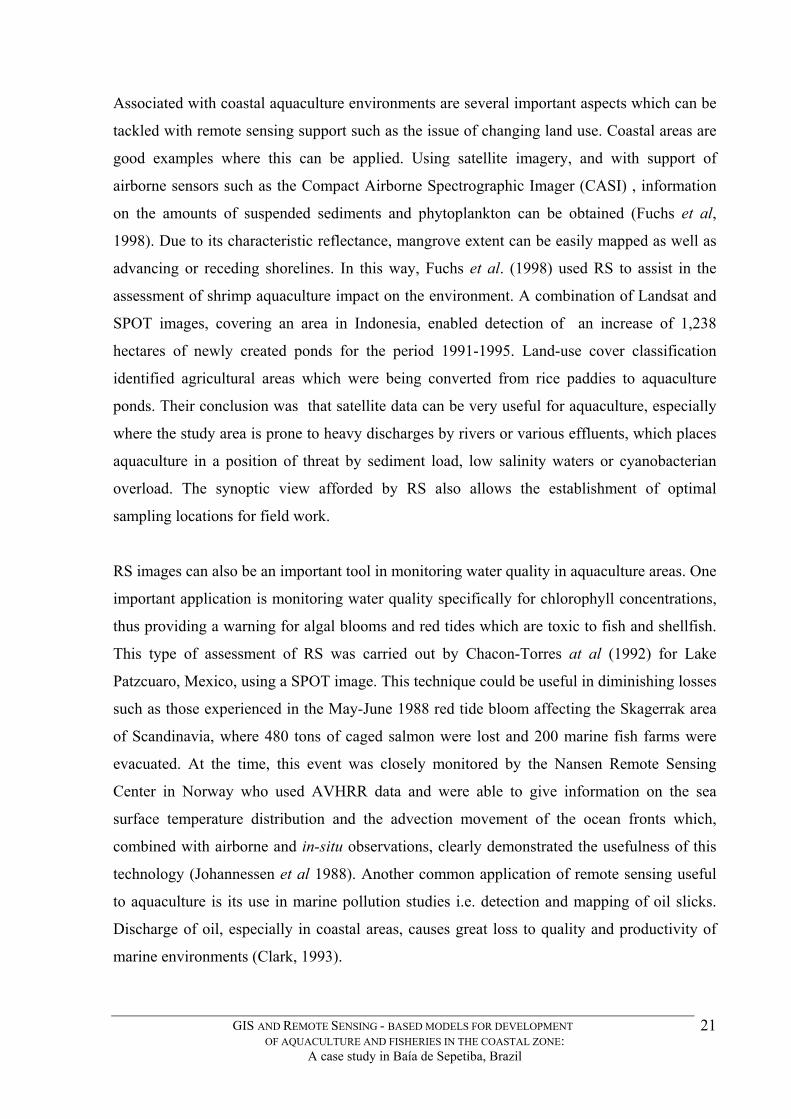
Associated with coastal aquaculture environments are several important aspects which can be

tackled with remote sensing support such as the issue of changing land use. Coastal areas are

good examples where this can be applied. Using satellite imagery, and with support of

airborne sensors such as the Compact Airborne Spectrographic Imager (CASI) , information

on the amounts of suspended sediments and phytoplankton can be obtained (Fuchs et al,

1998). Due to its characteristic reflectance, mangrove extent can be easily mapped as well as

advancing or receding shorelines. In this way, Fuchs et al. (1998) used RS to assist in the

assessment of shrimp aquaculture impact on the environment. A combination of Landsat and

SPOT images, covering an area in Indonesia, enabled detection of an increase of 1,238

hectares of newly created ponds for the period 1991-1995. Land-use cover classification

identified agricultural areas which were being converted from rice paddies to aquaculture

ponds. Their conclusion was that satellite data can be very useful for aquaculture, especially

where the study area is prone to heavy discharges by rivers or various effluents, which places

aquaculture in a position of threat by sediment load, low salinity waters or cyanobacterian

overload. The synoptic view afforded by RS also allows the establishment of optimal

sampling locations for field work.

RS images can also be an important tool in monitoring water quality in aquaculture areas. One

important application is monitoring water quality specifically for chlorophyll concentrations,

thus providing a warning for algal blooms and red tides which are toxic to fish and shellfish.

This type of assessment of RS was carried out by Chacon-Torres at al (1992) for Lake

Patzcuaro, Mexico, using a SPOT image. This technique could be useful in diminishing losses

such as those experienced in the May-June 1988 red tide bloom affecting the Skagerrak area

of Scandinavia, where 480 tons of caged salmon were lost and 200 marine fish farms were

evacuated. At the time, this event was closely monitored by the Nansen Remote Sensing

Center in Norway who used AVHRR data and were able to give information on the sea

surface temperature distribution and the advection movement of the ocean fronts which,

combined with airborne and in-situ observations, clearly demonstrated the usefulness of this

technology (Johannessen et al 1988). Another common application of remote sensing useful

to aquaculture is its use in marine pollution studies i.e. detection and mapping of oil slicks.

Discharge of oil, especially in coastal areas, causes great loss to quality and productivity of

marine environments (Clark, 1993).



21

With the use of RS images it is possible to greatly enhance a GIS-assisted aquaculture or

fisheries planning project as RS data can be used to identify and quantify a range of important

environmental characteristics of study areas. Some of these are water related such as:

bathymetry, suspended solids, surface temperature, chlorophyll a, salinity, total phosphorus

and current direction. In coastal areas, important thematic maps comprise cover type on

adjacent land and islands including vegetation types such as mangroves, wetlands, seagrass

reef flats, macroalgae etc. (Clark, 1993, Meaden and Chi, 1996).

GIS has potential for promoting the regulation of fisheries. There is the need to guarantee the

sustainability of fish stocks so as to ensure the maintenance of the fishing industry and its

back-up industrial sector and ensure the continuance of supply (Meaden and Chi, 1996).

There are still very few examples of direct integration of RS and GIS for fisheries support.

The first mention of a GIS applied to fisheries was a workshop held in Lybia by FAO for the

development of a GIS and Marine Fisheries (Meaden, 1994). Meaden and Chi (1996),

elaborated a document which considers many aspects relative to the use of GIS applications in

marine fisheries. This document also includes case studied of GIS applied to marine fisheries

and coastal zone resources management. The research applying GIS for fisheries exploitation

and management is confirmed in a recent paper by Meaden and Kemp (1997) who have

recently designed an integrated Fisheries Computer Aided Monitoring system called

FISHCAM, which integrates a GIS (ArcView) and a GPS with a relational database which

may be housed in an on-board computer. The proposal is ambitious but has definite

advantages concerning monitoring catches, their quantities and precise geographic locations

as well as providing new information which can be used to integrate fishing data with

environmental data. RS images from platforms such as Landsat, SPOT and AVHRR can

easily be integrated in this system, potentially increasing FISHCAM’s usefulness to both

fishermen and fisheries managers. In the same way, Junior et al. (1998) are developing a

skipjack tuna (Katswonus pelamis) fisheries GIS using SPRING-GIS, a freeware software

developed by Instituto Nacional de Pesquisas Espaciais in Brazil. Skipjack tuna is an

important pelagic fishery in the Southwestern Atlantic. The work carried out so far has

applied AVHRR images, treated to generate surface temperature charts (SST), which are

translated into fishing charts with an accompanying oceanographic bulletin for the guidance

of skipjack tuna capture fishing fleet.



22

Skippers are encouraged to record actual surface temperature, quantity fished, and geographic

position for feedback into the database. Feedback which supports the skipjack tuna locating

GIS model so far has proved far from ideal. Similar work is being carried out in the Canary

Islands by the Instituto Español de Oceanografia by Ariz et al. (unpublished) for bigeye tuna

Thunnus obesus. Interpretations of SST images derived from AVHRR show that higher

landings of bigeye tuna correlate more strongly with interfaces of, and pockets of, warmer

waters and upwelling water. Tuna are visual predators and, due to their physiological

characteristics, prefer water of higher temperature, high oxygen concentration and low level

of turbidity, to prey successfully (Ramos et al., 1996).

Some important coastal fisheries and shrimp resources are associated with seagrass meadows.

Ferguson and Korfmacher (1997) used RS and GIS for management of seagrass meadows in

North Carolina, USA. They found that spatial monitoring of seagrass meadows supported by

integration of Landsat TM image gave satisfactory results being regarded as cheaper than

would be possible with aerial photographs.

Mangroves are important coastal resources associated with several fisheries. Green et al

(1996) have summarised several remote sensing techniques for mangrove mapping which

include Landsat and SPOT sensors. The authors present a new image processing method for

mangroves which combines the most desirable characteristics of both sensors, creating a

seven band image with a 10 m spatial resolution.

Primary productivity in coastal waters is also a key factor in siting aquaculture operations. A

strong indication of productivity is phytoplankton abundance measured as chlorophyll a

concentration. Planktonic matter in surface waters is readily detected by remote sensing due

to the strong spectral signature of chlorophyll a. Sea water can be divided into two classes:

Case 1 water and Case 2 water (Sathyendranath and Morel 1983). Biomass can be estimated

from chlorophyll a measurements obtained by remote sensing, but in coastal zones, (Case 2

waters), this is more difficult, due to the amounts of suspended sediments and gilvin (yellow

colour determined by absorbance at 440 nm) (Clark, 1993).



23

This type of work is developing (Bagheri and Dios, 1990; Braga et al. 1993; Costa et al 1998;

Ekstrand, 1992; Forster et al. 1993; Pattiaratchi et al. 1994; Tassan and Ribera d' Alcala 1993;

Baban, 1997) and is currently based on better RS support, i.e. SeaWifs, a new instrument

which has capacity for observations of sea reflectances (SeaWIFS, 1999). Determining a

correlation for chlorophyll a concentration and the digital value from an RS image demands

calibration with values observed in the field for the study area. Table 1.2 summarises some

examples of correlations found for chlorophyll a and surface reflectance.

Table 1. 2. Algorithms developed for extracting Chlorophyll a concentrations from Landsat Thematic Mapper bands. TM1 = band 1, TM2 = band 2, TM3 = band 3.

AUTHOR STUDY AREA ALGORITHM

Pattiratchi et al. 1994 Cockburn Sound, Australia

Chl a (µg l –1) = 0.302 – 0.1 TM1 + 0.234 TM3

Ekstrand, 1992 Stockholm, Sweden

Chl a (µg l –1) = 116.78 + - 31.19(TM1/log TM3 + 1)

Costa, 1998 Ubatuba, Brazil Chl a (µg l –1) = 0.060914 + 0.109172 TM2 + 0.214841 TM3

Baban, 1997 Norfolk, UK Chl a (µg l –1) = -770+ 4768 * (TM3/TM1) – 24.6 (TM2+TM3)/2

Chlorophyll a and inorganic sediments are not separable and suspended sediments, which

dominate the total reflectance, behave as a broad band making inshore determinations of

chlorophyll a complex (Baban, 1997).

Some of these can be incorporated into the GIS for their value as biological indicators within

a sub model, or as areas restricted due to conservation measures. Hazard prevention can be

achieved by using the marine pollution detection capability, e.g. oil slicks and toxic algal

blooms. Since RS images can be obtained on at least a monthly basis, they also form an

important reference image library allowing time-series studies.



24

1.5 - Aims and objectives of this thesis

The aim of this research work was to address two principal questions:

1. Can GIS supported by Remote Sensing, be used to predict promising locations for

coastal aquaculture development in Sepetiba Bay, Rio de Janeiro ? If so, what would

be the area extent and production potential ?

2. What are the economic consequences of this development in terms of job creation and

natural resource exploitation?

In order to answer these questions, three aquaculture species were examined: Two species of

commonly cultivated filter feeding marine organisms native to Sepetiba Bay, and one exotic

marine shrimp, widely cultured throughout Brazil:

1. Perna perna the brown mussel which is found in many coastal areas along the Rio de

Janeiro coastline and has a mature industry base in Southern Brazil.

2. Crassostrea rhizophorae the mangrove oyster which is found commonly throughout

the bay and is a promissing potential species for warmer latitudes of Brazil, where

Crassostrea gigas, the japanese oyster does not fare well.

3. Litopenaeus vannamei a marine shrimp, native to Equador and Colombia, which

enabled the development of shrimp farming into an important industry in Latin

America and now the predominant cultured species in Brazil from North to South.

It is expected that the fulfilment of these aims will contribute to efforts already under way by

the state environment secretariat (SEMA) who is currently developing the coastal zone

management plan (GERCO), the state fisheries office (FIPERJ) in promoting sustainable local

aquaculture development and the agriculture extension service (EMATER) by showing areas

with potential aquaculture development to local stakeholders.



25

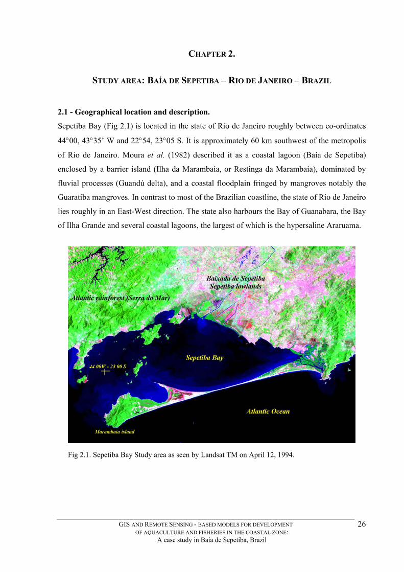
CHAPTER 2.

STUDY AREA: BAÍA DE SEPETIBA – RIO DE JANEIRO – BRAZIL

2.1 - Geographical location and description.

Sepetiba Bay (Fig 2.1) is located in the state of Rio de Janeiro roughly between co-ordinates

44°00, 43°35’ W and 22°54, 23°05 S. It is approximately 60 km southwest of the metropolis

of Rio de Janeiro. Moura et al. (1982) described it as a coastal lagoon (Baía de Sepetiba)

enclosed by a barrier island (Ilha da Marambaia, or Restinga da Marambaia), dominated by

fluvial processes (Guandú delta), and a coastal floodplain fringed by mangroves notably the

Guaratiba mangroves. In contrast to most of the Brazilian coastline, the state of Rio de Janeiro

lies roughly in an East-West direction. The state also harbours the Bay of Guanabara, the Bay

of Ilha Grande and several coastal lagoons, the largest of which is the hypersaline Araruama.

Fig 2.1. Sepetiba Bay Study area as seen by Landsat TM on April 12, 1994.



26

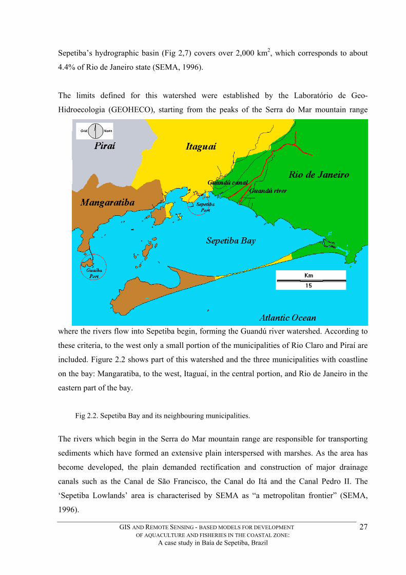
Sepetiba’s hydrographic basin (Fig 2,7) covers over 2,000 km2, which corresponds to about

4.4% of Rio de Janeiro state (SEMA, 1996).

The limits defined for this watershed were established by the Laboratório de Geo-

Hidroecologia (GEOHECO), starting from the peaks of the Serra do Mar mountain range

where the rivers flow into Sepetiba begin, forming the Guandú river watershed. According to

these criteria, to the west only a small portion of the municipalities of Rio Claro and Piraí are

included. Figure 2.2 shows part of this watershed and the three municipalities with coastline

on the bay: Mangaratiba, to the west, Itaguaí, in the central portion, and Rio de Janeiro in the

eastern part of the bay.

Fig 2.2. Sepetiba Bay and its neighbouring municipalities.

The rivers which begin in the Serra do Mar mountain range are responsible for transporting

sediments which have formed an extensive plain interspersed with marshes. As the area has

become developed, the plain demanded rectification and construction of major drainage

canals such as the Canal de São Francisco, the Canal do Itá and the Canal Pedro II. The

‘Sepetiba Lowlands’ area is characterised by SEMA as “a metropolitan frontier” (SEMA,

1996).



27

During the last decades the region has been settled in a series of ‘suburban rings’ around Rio

de Janeiro’s metropolitan zone intermingling areas of high population density with diluted

urbanization in the midst of several real estate ventures which are still awaiting land

valuation.

The fact that Sepetiba is served by important road and rail links between the neighboring

states of São Paulo and Minas Gerais confers upon it a strategic position. However this

strategic position is also defined by industrial-urban concentrations outwith the Sepetiba

Lowlands (Rio de Janeiro, São Paulo, Minas Gerais), which has induced strip development

using the area as a ‘passageway’ or goods export-import corridor rather than as an

‘environmental unit’. The development plan for the expansion of the Port of Sepetiba is in

progress and will play an important role in the local economy and environment.

2.2 - The Port

The port of Sepetiba is located in

the central part of Sepetiba Bay

on the northern shore (Fig 2.3) It

was inaugurated in 1982, and

began its activities receiving coal

and alumina. It is strategically

located as it is within a 500 km

radius of many industrial and

commercial companies in Brazil,

which account for about 70% of

the Brazilian GNP (CDRJ,

1999).

Fig 2.3. Port of Sepetiba. Final planned layout. (From CDRJ, 1999).

The port currently has a handling capacity for 7 million tons of cargo and is being expanded

to enable ships of up to 150,000 tons to dock and move an estimated 18-20 million tons/yr. of

cargo including iron ore, coal, grains and additionally an estimated one million containers. It

is projected to be the only Hubport in the south Atlantic concentrating cargo. It’s design

include ‘Roll-on Roll-off’ facilities (Fig 2.3).



28

The Port of Sepetiba has demanded a global investment value US$350 million of which

US$150 million are loaned from the Inter-American Development Bank. The project is a

partnership between the Brazilian Development Bank (BNDES) and private initiative and its

completion date was scheduled for September 1998. The port’s characteristics are described

by CDRJ (1999). These include an access channel 22 km long, 200m wide and on average

15m deep. The docking pier is 540 long, 40 m wide and can berth simultaneously two 90,000t

and two 45,000t cargo ships (CDRJ, 1999). The access area has two silos for holding alumina

with a static capacity of 30,630 t.

2.3 - Temperature

Most of the coastal area of Sepetiba has a mean annual temperature above 23.5o C as can be

seen in Figure 2.4. Higher mean annual temperatures occur in the lowland areas reaching over

23.5o C in the central region to its highest values (>24o C) between the Pedra Branca e

Mendanha mountains. With increasing altitude, temperatures decrease and are less than 17o C

in the upper parts of Mazomba and Couto in the Tinguá range.

Fig 2.4. Mean annual temperatureAdapted from SEMA (1996).



29

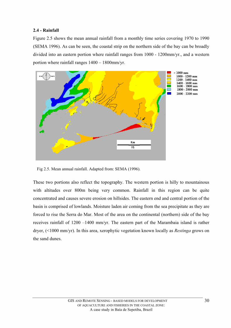
2.4 - Rainfall

Figure 2.5 shows the mean annual rainfall from a monthly time series covering 1970 to 1990

(SEMA 1996). As can be seen, the coastal strip on the northern side of the bay can be broadly

divided into an eastern portion where rainfall ranges from 1000 - 1200mm/yr., and a western

portion where rainfall ranges 1400 – 1800mm/yr.

Fig 2.5. Mean annual rainfall. Adapted from: SEMA (1996).

These two portions also reflect the topography. The western portion is hilly to mountainous

with altitudes over 800m being very common. Rainfall in this region can be quite

concentrated and causes severe erosion on hillsides. The eastern end and central portion of the

basin is comprised of lowlands. Moisture laden air coming from the sea precipitate as they are

forced to rise the Serra do Mar. Most of the area on the continental (northern) side of the bay

receives rainfall of 1200 –1400 mm/yr. The eastern part of the Marambaia island is rather

dryer, (<1000 mm/yr). In this area, xerophytic vegetation known locally as Restinga grows on

the sand dunes.



30

2.5 - Climate 2.5.1 - Köppen Climate Classification

SEMA (1996) proposed three different climatic classes in Sepetiba (Fig 2.6) based on the

Köppen classification (Table 2.1) where monthly precipitation and temperatures are related.

Fig 2.6. Köppens’s climatic classification for Sepetiba Bay. Adapted from SEMA (1996).

Acording to this system, Sepetiba basin is divided between three climatic domains, the

predominant of which is Aw mostly affecting the lowlands and lower reaches of the Serra do

Mar which flanks it to the west and other hillsides towards the east. Aw is characterised by a

slight drought in the winter months and higher average temperatures (above 18o C) all year

round. The second type, Af, mostly affects the islands and western reaches of the bay.

It is the type of climate with higher year-round precipitation and also higher temperatures. Cf

climate (cool and wet) is confined mostly away from the coastline and at higher altitudes.



31

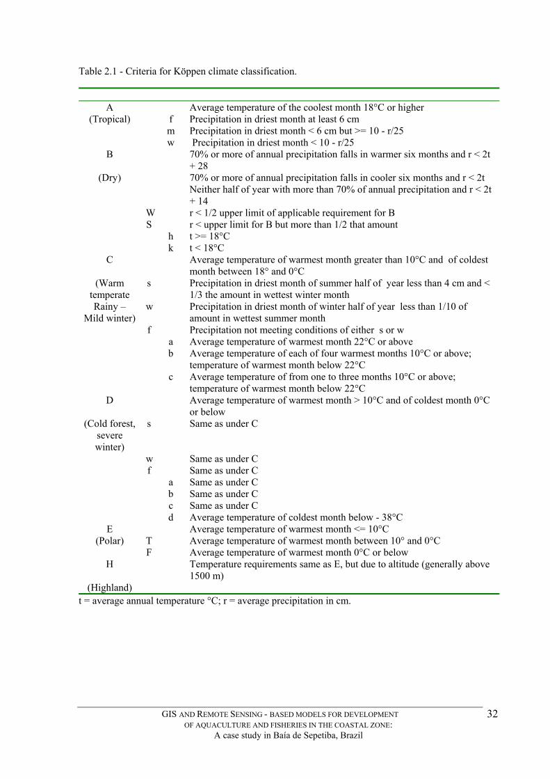
Table 2.1 - Criteria for Köppen climate classification.

A Average temperature of the coolest month 18°C or higher

(Tropical) f Precipitation in driest month at least 6 cm m Precipitation in driest month < 6 cm but >= 10 - r/25 w Precipitation in driest month < 10 - r/25

B 70% or more of annual precipitation falls in warmer six months and r < 2t + 28

(Dry) 70% or more of annual precipitation falls in cooler six months and r < 2t Neither half of year with more than 70% of annual precipitation and r < 2t

+ 14 W r < 1/2 upper limit of applicable requirement for B S r < upper limit for B but more than 1/2 that amount h t >= 18°C k t < 18°C

C Average temperature of warmest month greater than 10°C and of coldest month between 18° and 0°C

(Warm temperate

s Precipitation in driest month of summer half of year less than 4 cm and < 1/3 the amount in wettest winter month

Rainy – Mild winter)

w Precipitation in driest month of winter half of year less than 1/10 of amount in wettest summer month

f Precipitation not meeting conditions of either s or w a Average temperature of warmest month 22°C or above b Average temperature of each of four warmest months 10°C or above;

temperature of warmest month below 22°C c Average temperature of from one to three months 10°C or above;

temperature of warmest month below 22°C D Average temperature of warmest month > 10°C and of coldest month 0°C

or below (Cold forest,

severe winter)

s Same as under C

w Same as under C f Same as under C a Same as under C b Same as under C c Same as under C d Average temperature of coldest month below - 38°C

E Average temperature of warmest month <= 10°C (Polar) T Average temperature of warmest month between 10° and 0°C

F Average temperature of warmest month 0°C or below H Temperature requirements same as E, but due to altitude (generally above

1500 m) (Highland)

t = average annual temperature °C; r = average precipitation in cm.



32

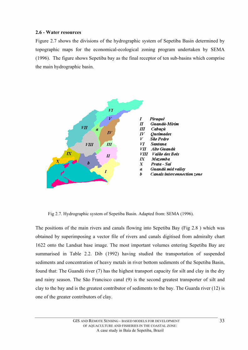
2.6 - Water resources

Figure 2.7 shows the divisions of the hydrographic system of Sepetiba Basin determined by

topographic maps for the economical-ecological zoning program undertaken by SEMA

(1996). The figure shows Sepetiba bay as the final receptor of ten sub-basins which comprise

the main hydrographic basin.

Fig 2.7. Hydrographic system of Sepetiba Basin. Adapted from: SEMA (1996).

The positions of the main rivers and canals flowing into Sepetiba Bay (Fig 2.8 ) which was

obtained by superimposing a vector file of rivers and canals digitised from admiralty chart

1622 onto the Landsat base image. The most important volumes entering Sepetiba Bay are

summarised in Table 2.2. Dib (1992) having studied the transportation of suspended

sediments and concentration of heavy metals in river bottom sediments of the Sepetiba Basin,

found that: The Guandú river (7) has the highest transport capacity for silt and clay in the dry

and rainy season. The São Francisco canal (9) is the second greatest transporter of silt and

clay to the bay and is the greatest contributor of sediments to the bay. The Guarda river (12) is

one of the greater contributors of clay.



33

Fig 2.8. Main river and canal outflows into Baía de Sepetiba. 1. Rio do Portinho 2. Rio Piracão 3. Rio Piraí 4. Rio Piraquê 5. Rio do Ponto 6. Canal do Itá 7. Rio Guandú 8. Canal do Guandú 9. Canal São Francisco 10. Canal Sto Agostinho 11. Rio Itaguaí 12. Rio da Guarda 13. Saco do Engenho 14. Rio Mazomba 15. Rio Cação 16. Rio Monjolo 17. Rio Itinguiçú 18. Rio Corumbí 19. Rio Prata 20. Rio Saí 21. Rio do Saco.

The Piraquê river (4) although one of the smallest, had a significant contribution of

suspended materials, mostly due to intense urbanization process along its watershed. The river

Cação (15) showed consistently high levels of Zn (417µgl-1 ) and Cd 2 µgl-1 . This fact is most

probably related to it’s proximity to the Ingá Zinc ingot manufacturing plant and the Port of

Sepetiba, which normally imports mineral coal for industries in the area including a thermo-

electric plant.

Table 2.2. Characteristics of main freshwater contributors to Sepetiba Bay (adapted from Dib, 1992).

NAME VELOCITY m s -1

DEPTH M

WIDTH m VOLUME m3 s-1

SILTE g l-1

CLAY gl-1

Rio Guandú 0.91 5.7 127 341.99 0.075 0.2 Canal de São Francisco 0.73 6.3 141 278.45 0.07 0.22 Rio da Guarda 0.45 3.6 35.5 36.58 0.09 0.26 Canal do Guandú 0.9 2.1 19 30.15 0.3 0.39 Valão dos Bois 0.45 2 39.3 28.31 0.07 0.4 Rio Cai-tudo 0.4 2.8 43 27.58 0.055 0.23 Rio Piraquê 0.4 2.9 23.8 17 0.045 0.9 Rio Cação 0.71 1.1 15.3 9.27 0.1 0.13



34

2.7 - Soils

The predominant soil types in the coastal lowlands of the bay are gleysols and planosols

(SEMA, 1996) (Fig 2.9). Gleysol soils have a texture (Tables 2.3 and 2.4) which make them

prone to flooding and usually costly to improve. Although the natural fertility of these young

sediments is usually high, they are heavy clay soils, and therefore are less suitable for crops

with small seeds. Over the South American continent, they are frequently used for extensive

cattle grazing during the season when these soils are not inundated. Otherwise, they may be

used for rice cultivation. Near sea level, such as in Sepetiba, crops include sugarcane, rice,

bananas, cocoa and coffee. In river valleys near urban centres the soils are intensively used for

horticulture, as in the rural areas of Campo Grande, Itaguaí and Santa Cruz. They are suitable

for rice, jute, sugarcane and good pastures but must be drained (FAO-Unesco, 1971).

Planosols are also found in the urban area of Sepetiba. They are characterised by a heavy

texture, impermeable B horizon, and inundation for part of the year. They are not very

suitable for crops as the subsoil is impervious and quite dificult to break. They are good for

rice cultivation, although this is not practised in Sepetiba. Both soils types may have low

content of sodium salts.

Table 2.3. Principal characteristics of Eutric Gleysol (saline phase) for South America. Adapted from FAO- World Soils Map.

ORGANIC MATTER SOLUBLE SALTS

HORIZON DEPTH %C %N C/N PH SO4 -- CL

-- TEXTURE

A 0-10 4.1 0.34 12 5.2 0.3 2.2 Silty clay loam Cg1 -38 1.0 0.21 5 7.1 0.9 3.8 Silty clay Cg2 -60 0.7 0.04 17 6.6 1.2 3.3 Silty clay Cg3 -112 1.6 0.13 12 6.2 2.0 2.5 Silty clay Cg4 -150 2.7 0.15 18 4.7 4.4 3.0 Silt loam

Table 2.4. Principal characteristics of Eutric Planosol for South America. Adapted from FAO- World Soils Map.

ORGANIC MATTER SOLUBLE SALTS

HORIZON DEPTH %C %N C/N PH - - TEXTURE A/E1 0-18 1.0 0.10 10 5.4 - - Sandy loam

E2 - 25 0.3 0.03 - 6.5 - - Sandy loam BE/Bt1 - 50 0.7 0.06 - 6.8 - - Clay

Bt2 - 65 0.4 0.04 - 7.5 - - Clay Bck -85 0.1 0.02 - 8.5 - - Clay loam C - 150+ 0 - - 7.5 - - Clay loam



35

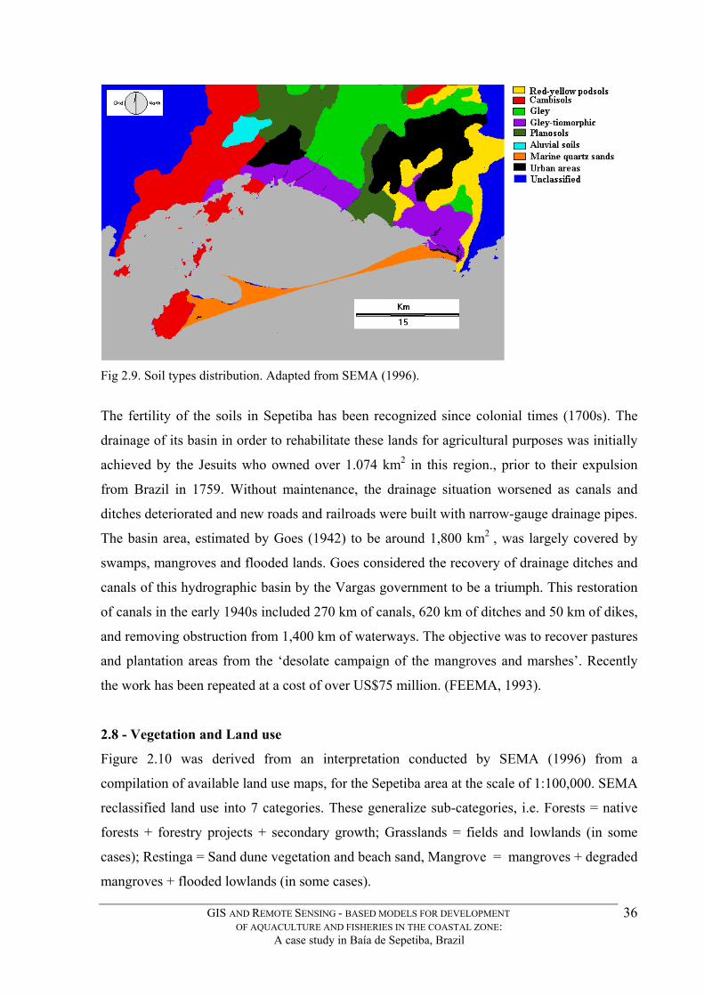
Fig 2.9. Soil types distribution. Adapted from SEMA (1996).

The fertility of the soils in Sepetiba has been recognized since colonial times (1700s). The

drainage of its basin in order to rehabilitate these lands for agricultural purposes was initially

achieved by the Jesuits who owned over 1.074 km2 in this region., prior to their expulsion

from Brazil in 1759. Without maintenance, the drainage situation worsened as canals and

ditches deteriorated and new roads and railroads were built with narrow-gauge drainage pipes.

The basin area, estimated by Goes (1942) to be around 1,800 km2 , was largely covered by

swamps, mangroves and flooded lands. Goes considered the recovery of drainage ditches and

canals of this hydrographic basin by the Vargas government to be a triumph. This restoration

of canals in the early 1940s included 270 km of canals, 620 km of ditches and 50 km of dikes,

and removing obstruction from 1,400 km of waterways. The objective was to recover pastures

and plantation areas from the ‘desolate campaign of the mangroves and marshes’. Recently

the work has been repeated at a cost of over US$75 million. (FEEMA, 1993).

2.8 - Vegetation and Land use

Figure 2.10 was derived from an interpretation conducted by SEMA (1996) from a

compilation of available land use maps, for the Sepetiba area at the scale of 1:100,000. SEMA

reclassified land use into 7 categories. These generalize sub-categories, i.e. Forests = native

forests + forestry projects + secondary growth; Grasslands = fields and lowlands (in some

cases); Restinga = Sand dune vegetation and beach sand, Mangrove = mangroves + degraded

mangroves + flooded lowlands (in some cases).



36

Fig 2.10. Land use in the study area. Adapted from: SEMA (1996).

2.9 - Conservation areas

Sepetiba Basin has several legal environmental conservation units shown in Figure 2.11.

These include important two state parks, one to the eastern end of the bay, the . Parque

Estadual da Pedra Branca (2) is established as a Permanent Preservation Area (APP) by

resolution CONAMA 05/85, (art.2 of the Brazilian Forestry Code), and is defined as

‘Ecological Reserve’. The park covers 12,500 ha and harbours remnant portions of Atlantic

(rain) Forest ecosystem. It overlooks the Guaratiba region, most notewothy for its well

developed mangroves, protected in the Reserva Biológica e Arqueológica de Guaratiba (1)

The reserve covers 2.800 ha which salt barrens and exuberant mangroves at the eastern end of

the Sepetiba bay. This area contains over 40 middens, locally known as sambaquís, which are

mounds of remnants left by ancient indiginous peoples the Tupi-Guaranís, containing mostly

seashells and artifacts. The presence of numerous middens along the Rio de Janeiro coastline

confirms the importance of shellfish as food source for native populations (Lamego, 1964).

The Parque Estadual das Serras do Madureira/Mendanha (3) is still in the proposal stage

and will protect about 6.000 ha of forested areas.



37

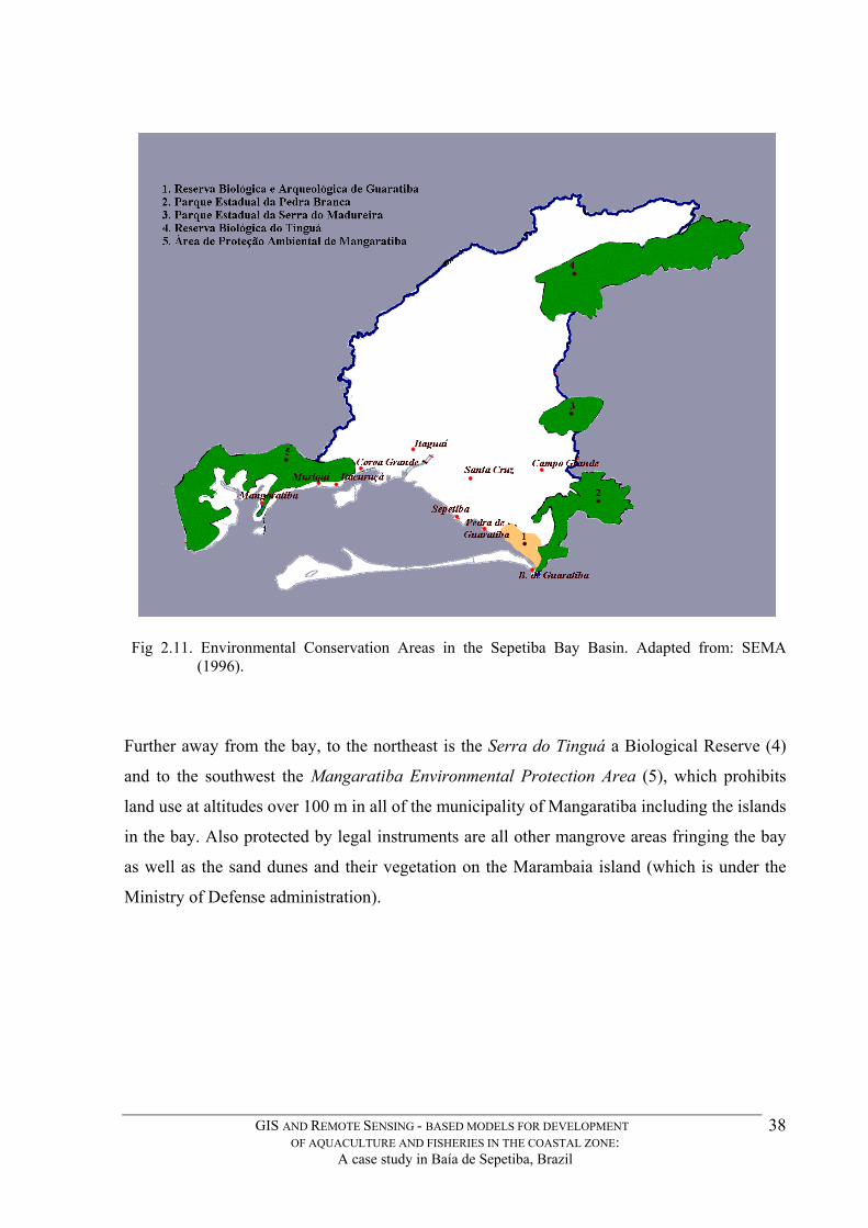
Fig 2.11. Environmental Conservation Areas in the Sepetiba Bay Basin. Adapted from: SEMA

(1996).

Further away from the bay, to the northeast is the Serra do Tinguá a Biological Reserve (4)

and to the southwest the Mangaratiba Environmental Protection Area (5), which prohibits

land use at altitudes over 100 m in all of the municipality of Mangaratiba including the islands

in the bay. Also protected by legal instruments are all other mangrove areas fringing the bay

as well as the sand dunes and their vegetation on the Marambaia island (which is under the

Ministry of Defense administration).



38

2.10 - Geomorphology and Oceanography

Lamego (1944) proposed the generally accepted explanation for Sepetiba Bay’s origin, as

being a result of the coastal current moving in a northeasterly direction headed for the

Guaratiba headland. This is a classical example of a barrier beach developing landward from a

sea island as described in Garrison, (1999) and illustrated in Figure 2.12. An emergent

tombolo protruded from Marambaia island, being fed by river-borne sediments from the

adjacent coastal plain, mainly the Guandú and Itaguaí rivers. The shallow coastal waters allied

with an effective sediment barrier provided by the islands chain of Madeira, Itacuruçá,

Furtada, Jaguanum and Marambaia (and several other smaller ones) allowed the tombolo to

bridge and connect to the continent. As it attained considerable size, wind helped it to advance

and build sand dunes. Eventually the newly formed barrier beach took an West-East direction

accomodating for a new secondary internal current. So far, the eastern end of Sepetiba bay,

Guaratiba, has not closed. The Canal do Bacalhau channel provides fresh seawater exchange

from that end. The barrier beach today shelters the internal waters of the semi-enclosed bay

and a newer spit has formed from the main barrier beach towards Jaguanum island.

Ponçano (1976), who studied in detail the sedimentation of Sepetiba Bay, took a different

view and suggests that river-borne sediments were less important to the formation of the

barrier island than attributed by Lamego. He concluded that another spit departed the eastern

end of the bay and that with action of coastal eddies brought sediments of coastal shelf origin

to feed sand bars which formed the bulk of the barrier beach. Both sand spits eventually

joined, closing the bay from open water exposure. In any case, the result of these processes

has led to the formation of a reasonably well protected, semi-enclosed coastal lagoon, which

is fed by nutrients brought through rivers draining a a large (over 2,000 km2 ) basin.



39

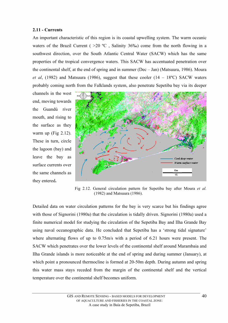
2.11 - Currents

An important characteristic of this region is its coastal upwelling system. The warm oceanic

waters of the Brazil Current ( >20 ºC , Salinity 36‰) come from the north flowing in a

southwest direction, over the South Atlantic Central Water (SACW) which has the same

properties of the tropical convergence waters. This SACW has accentuated penetration over

the continental shelf, at the end of spring and in summer (Dec – Jan) (Matsuura, 1986). Moura

et al, (1982) and Matsuura (1986), suggest that these cooler (14 – 18ºC) SACW waters

probably coming north from the Falklands system, also penetrate Sepetiba bay via its deeper

channels in the west

end, moving towards

the Guandú river

mouth, and rising to

the surface as they

warm up (Fig 2.12).

These in turn, circle

the lagoon (bay) and

leave the bay as

surface currents over

the same channels as

they entered.

Fig 2.12. General circulation pattern for Sepetiba bay after Moura et al. (1982) and Matsuura (1986).

Detailed data on water circulation patterns for the bay is very scarce but his findings agree

with those of Signorini (1980a) that the circulation is tidally driven. Signorini (1980a) used a

finite numerical model for studying the circulation of the Sepetiba Bay and Ilha Grande Bay

using naval oceanographic data. He concluded that Sepetiba has a ‘strong tidal signature’

where alternating flows of up to 0.75m/s with a period of 6.21 hours were present. The

SACW which penetrates over the lower levels of the continental shelf around Marambaia and

Ilha Grande islands is more noticeable at the end of spring and during summer (January), at

which point a pronounced thermocline is formed at 20-50m depth. During autumn and spring

this water mass stays receded from the margin of the continental shelf and the vertical

temperature over the continental shelf becomes uniform.



40

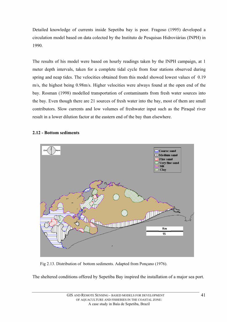
Detailed knowledge of currents inside Sepetiba bay is poor. Fragoso (1995) developed a

circulation model based on data colected by the Instituto de Pesquisas Hidroviárias (INPH) in

1990.

The results of his model were based on hourly readings taken by the INPH campaign, at 1

meter depth intervals, taken for a complete tidal cycle from four stations observed during

spring and neap tides. The velocities obtained from this model showed lowest values of 0.19

m/s, the highest being 0.98m/s. Higher velocities were always found at the open end of the

bay. Rosman (1998) modelled transportation of contaminants from fresh water sources into

the bay. Even though there are 21 sources of fresh water into the bay, most of them are small

contributors. Slow currents and low volumes of freshwater input such as the Piraquê river

result in a lower dilution factor at the eastern end of the bay than elsewhere.

2.12 - Bottom sediments

Fig 2.13. Distribution of bottom sediments. Adapted from Ponçano (1976).

The sheltered conditions offered by Sepetiba Bay inspired the installation of a major sea port.



41

As the life span of a port complex ultimately depends on sediment dynamics and rate of

changes (Ponçano, 1976), a study was made by Geomecânica S.A. using a 2 km x 2 km grid,

where 273 surface sediment samples were collected from the bay and adjacent areas just

outside. The result is a sediment distribution map (Fig 2.13) classified according to the

Wentworth’s scheme (Table 2.5), which clearly shows that the central and eastern portions of

the bay are dominated by bottom sediments composed mostly of silt, of terrigenous origin.

The western end of the bay is dominated by medium to coarse sands, a confirmation of the

existence of swift bottom currents (Tait, 1981). This knowledge of the bottom sediment

distribution can be useful for studies considering distribution of benthic comunities (Ponçano,

1976). More information on bottom sediment quality and distribution has recently become

available from a siesmic profiling campaign carried out by FEEMA (1997).

Table 2.5. Wentworth Classification of Particle Grades and Phi Scale (From Tait, 1981)

GRADE NAME PARTICLE SIZE (MM) PHI UNITS

Boulder > 256 Beyond – 8.0 Cobble 256 → 64 -8.0 → - 8.0 Pebble 64 → 4 -6 → -2.0 Granule 4 → 2 -2.0 → -1.0 Very coarse sand 2 → 1 -1.0 → 0 Coarse sand 1 → 0.5 0 → 1.0 Medium sand 0.5 → 0.25 1.0 → 2.0 Very fine sand 0.125 → 0.0625 2.0 → 3.0 Silt 0.0625 → 0.0039 4.0 → 8.0 Clay > 0.0039 Beyond 8.0 2.13 - Water Quality

The water quality data history for Sepetiba Bay is very poor. A series of cartograms depicting

water surface temperature, salinity, dissolved oxygen, chlorophyll a and amonia contents was

produced by SEMA (1996) based on average values compiled by FEEMA as a result of a

major water quality sampling campaign carried out in 1990. Sepetiba Bay has a marked

estuarine characteristic, and as Tait (1981) points out, estuarine waters “are not a simple

dilution of seawater”.



42

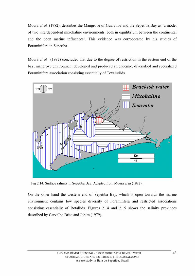
Moura et al. (1982), describes the Mangrove of Guaratiba and the Sepetiba Bay as ‘a model

of two interdependent mixohaline environments, both in equilibrium between the continental

and the open marine influences’. This evidence was corroborated by his studies of

Foraminifera in Sepetiba.

Moura et al. (1982) concluded that due to the degree of restriction in the eastern end of the

bay, mangrove environment developed and produced an endemic, diversified and specialized

Foraminifera association consisting essentially of Texaluriids.

Fig 2.14. Surface salinity in Sepetiba Bay. Adapted from Moura et al (1982).

On the other hand the western end of Sepetiba Bay, which is open towards the marine

environment contains low species diversity of Foraminfera and restricted associations

consisting essentially of Rotaliids. Figures 2.14 and 2.15 shows the salinity provinces

described by Carvalho Brito and Jobim (1979).



43

Fig 2.15. Bottom salinity, adapted from Moura et al (1982).

These are divided into 3 provinces: brackish water 5-18‰, mixohaline 18-30‰, and seawater

30-40‰. These surface and bottom salinity provinces have variable geographical limits on a

diurnal basis.

2.14 - Water Colour

Few surveys in Sepetiba have been comprehensive in collecting simultaneously the many

water quality parameters necessary for better understanding its dynamics. Water colour

changes markedly in estuarine waters as a function of several factors. Oliveira, (1971)

surveyed over 100 points in the bay using the total apparent color classification scheme

described in Sverdrup, (1948). The results are illustrated in Figure 2.16. Oliveira judged this

method to be important for shallow waters because it translated an association of organisms

related to a specific water colour over a period of time. The colors identified in Oliveira’s

study were correlated with supplementary information regarding their relevance to fisheries,

which was obtained with interviewed fishermen. Specifically important to them were colors

associating the presence of white shrimp in feeding behaviour over the muddy bottoms.



44

Fig 2.16. Water colour classification for Sepetiba bay waters. (Adapted from Oliveira, 1971).

According to the fishermen, the white shrimp create this type of colour by lifting bottom

sediments with their pereipods and peleopods as they search for prey and food particles.

Skates and rays are said to produce a different colour effect, as they disturb deeper and darker

coloured layers of sediments. Mullets are said to prefer waters with the agrifolium colour.

Oliveira supplemented these reports from the fishermen with biological samples taken

throughout the bay and their associated water colours. For example, waters corresponding to

moss green colour were associated with an abundance of white shrimp larvae. Other abundant

organisms such as blue-green algae, echinoderms, mullets, and benthic diatoms were also

associated with specific water colours.

2.15 - Aquaculture in Sepetiba

To date, state actions for aquaculture research, development and extension for Sepetiba Bay

have been disconcerted, alienating the coastal artisanal fisherman, an important stakeholder

who could potentially benefit from, and contribute to a well structured aquaculture and

fisheries development plan. In the past 20 years, a few aquaculture initiatives have started but

have been discontinued for a series of reasons.



45

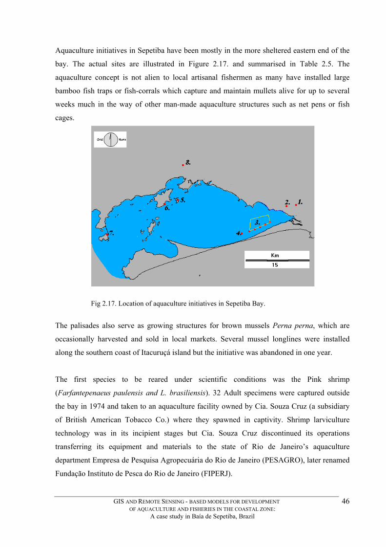
Aquaculture initiatives in Sepetiba have been mostly in the more sheltered eastern end of the

bay. The actual sites are illustrated in Figure 2.17. and summarised in Table 2.5. The

aquaculture concept is not alien to local artisanal fishermen as many have installed large

bamboo fish traps or fish-corrals which capture and maintain mullets alive for up to several

weeks much in the way of other man-made aquaculture structures such as net pens or fish

cages.

Fig 2.17. Location of aquaculture initiatives in Sepetiba Bay.

The palisades also serve as growing structures for brown mussels Perna perna, which are

occasionally harvested and sold in local markets. Several mussel longlines were installed

along the southern coast of Itacuruçá island but the initiative was abandoned in one year.

The first species to be reared under scientific conditions was the Pink shrimp

(Farfantepenaeus paulensis and L. brasiliensis). 32 Adult specimens were captured outside

the bay in 1974 and taken to an aquaculture facility owned by Cia. Souza Cruz (a subsidiary

of British American Tobacco Co.) where they spawned in captivity. Shrimp larviculture

technology was in its incipient stages but Cia. Souza Cruz discontinued its operations

transferring its equipment and materials to the state of Rio de Janeiro’s aquaculture

department Empresa de Pesquisa Agropecuária do Rio de Janeiro (PESAGRO), later renamed

Fundação Instituto de Pesca do Rio de Janeiro (FIPERJ).



46

Table 2.6. Main aquaculture initiatives in Sepetiba Bay region.

SPECIES

INITIATIVE

YEAR Farfantepenaeus paulensis and Penaeus brasiliensis) b

Cia. Souza Cruz 1973

F. paulensis and P. brasiliensis) a

Fundação Instituto de Pesca do Rio de Janeiro (FIPERJ) – successful larviculture, for stocking enhancement.

1974

Trachinotus spp.b Pereira & Magalhães, Cage culture (on-growing) of Pompano.

1978

Macrobrachium rosenbergiib

FIPERJ – post-larvae production 1984

M. rosenbergiib Hotel Charles – on growing freshwater prawns 1984 Mugil spp.a Japan International Cooperation Agency (JICA) funded

project. On-growing 1990

Perna pernab mussel longlines 1995 Crassostrea rhizophoraea FIPERJ – Larviculture only – spat production 1998 Penaeus schmittib Mineirações Brasileiras Reunidas (MBR) – shrimp cage

culture 1998

a. state run project b. private entrepreneurs

PESAGRO managed to spawn pink shrimp under its new lab conditions in 1975. (Thomas

and Cataldo de Castro, 1982). The post-larvae were put for on-growing in earthen ponds in

the Sepetiba area. However, in the subsequent years, PESAGRO switched from its research

emphasis focused on reproduction aspects of the native F. paulensis to that of the exotic

freshwater prawn, Macrobrachium rosenbergii. Due to the relative technical ease of

reproduction and on-growing aspects of this species, it remained as the main concern of this

state-run lab for several years. Millions of M. rosenbergii post-larvae were produced and

shipped to all parts of the state, as well as to other states in Brazil, but only one site (Hotel

Charles) in the bay area is known to have engaged in semi-commercial on-growing.

Mineirações Brasileiras Reunidas is currently attempting cage culture of white shrimp

(P. schmitti) at Ilha da Guaíba (Scott, unpublished).

Subsequently, PESAGRO attempted cage-culture of mullets (Mugil spp.) with financial

support from the Japanese International Cooperation Agency (JICA). PESAGRO and its

Japanese cage-culture specialists selected a site, which coincidentally was close to the

artisanal fishermen fish corrals.



47

Due to a poor communication process, this technical attempt was met by the fishermen with

bitter hostility. They did not appreciate the state-project considering it an intrusion into their

affairs and a disregard for their ‘traditional’ rights to the area (Martino, unpublished).

Juvenile pompano (Trachinotus spp), a local species, was captured by Pereira & Magalhães

(personal communication) and used in on-growing trials in floating fish-cages at Ilha do

Martins. This was attempted in collaboartion with local fishermen from Ilha da Madeira, but

eventually failed as nets were severely damaged by puffer fish, which ate dead fish lying on

the bottom or entrapped in the mesh.

Recently (1998), FIPERJ has initiated spat production of local mangrove oysters (C.

rhizophorae). This is a first attempt at culturing a local native mollusc. The broodstock were

collected in the local mangroves of Guaratiba, conditioned in the FIPERJ aquaculture station

and oyster spat was produced.



48

CHAPTER 3.

MATERIALS AND METHODS

3.1 - Introduction

The studies undertaken in this research project can be broadly divided in two: a) laboratory

based and b) field based operations. It is important to recognise that these are different

working environments which require careful consideration and balance for overall best

results. Laboratory and field-based equipment have different functions and a good knowledge

of their capabilities and limitations is very important for the best development of the GIS

database. Ideally the field based and lab-based operations must work hand in hand.

Several types of field data needed to be collected ranging from observations on land-use,

vegetation cover, water and soil properties etc., and had to be stored in an organised way for

subsequent integration into the GIS database. Ideally, the time delay between field data

acquisition time and preliminary data processing in the GIS database should be minimal.

It was possible to reduce this time delay by ‘taking the laboratory to the field’ and using a

portable computer with GIS software installed. In this way, it was possible to add information

and data to the database, while navigating through the study area with a previously digitised

map or even remotely sensed images displayed as a backdrop in real time. In the early, data

gathering stages of the study this approach however was not available. Field based operations

relied upon notes taken during several field trips where information was input into tables

using printed reference maps and charts as well as geographic positions read from a hand held

GPS.

3.2 - Laboratory based operations

3.2.1 - Computers

All laboratory based operations were undertaken in the working environment of the

Geographical Information Systems and Applied Physiology (GISAP) facilities of the Institute

of Aquaculture (IoA), Stirling University. GISAP facilities include five dedicated GIS

workstations, which are networked to several servers on campus.



49

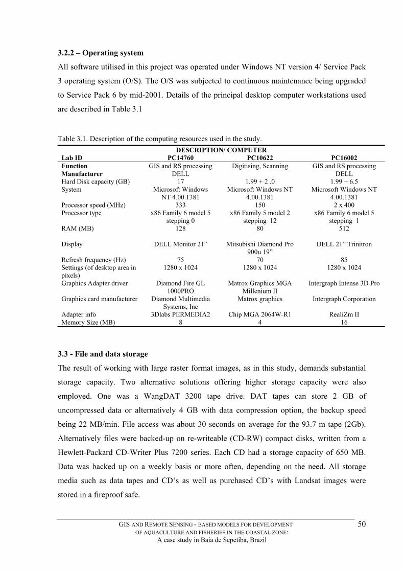
3.2.2 – Operating system

All software utilised in this project was operated under Windows NT version 4/ Service Pack

3 operating system (O/S). The O/S was subjected to continuous maintenance being upgraded

to Service Pack 6 by mid-2001. Details of the principal desktop computer workstations used

are described in Table 3.1

Table 3.1. Description of the computing resources used in the study. DESCRIPTION/ COMPUTER

Lab ID PC14760 PC10622 PC16002 Function GIS and RS processing Digitising, Scanning GIS and RS processing Manufacturer DELL DELL Hard Disk capacity (GB) 17 1.99 + 2 .0 1.99 + 6.5 System Microsoft Windows

NT 4.00.1381 Microsoft Windows NT

4.00.1381 Microsoft Windows NT

4.00.1381 Processor speed (MHz) 333 150 2 x 400 Processor type x86 Family 6 model 5

stepping 0 x86 Family 5 model 2

stepping 12 x86 Family 6 model 5

stepping 1 RAM (MB)

128 80 512

Display DELL Monitor 21” Mitsubishi Diamond Pro 900u 19”

DELL 21” Trinitron

Refresh frequency (Hz) 75 70 85 Settings (of desktop area in pixels)

1280 x 1024 1280 x 1024 1280 x 1024

Graphics Adapter driver Diamond Fire GL 1000PRO

Matrox Graphics MGA Millenium II

Intergraph Intense 3D Pro

Graphics card manufacturer Diamond Multimedia Systems, Inc

Matrox graphics Intergraph Corporation

Adapter info 3Dlabs PERMEDIA2 Chip MGA 2064W-R1 RealiZm II Memory Size (MB) 8 4 16

3.3 - File and data storage

The result of working with large raster format images, as in this study, demands substantial

storage capacity. Two alternative solutions offering higher storage capacity were also

employed. One was a WangDAT 3200 tape drive. DAT tapes can store 2 GB of

uncompressed data or alternatively 4 GB with data compression option, the backup speed

being 22 MB/min. File access was about 30 seconds on average for the 93.7 m tape (2Gb).

Alternatively files were backed-up on re-writeable (CD-RW) compact disks, written from a

Hewlett-Packard CD-Writer Plus 7200 series. Each CD had a storage capacity of 650 MB.

Data was backed up on a weekly basis or more often, depending on the need. All storage

media such as data tapes and CD’s as well as purchased CD’s with Landsat images were

stored in a fireproof safe.



50

The Sepetiba database comprised several raster images extracted or derived from a basic

Landsat image and vector files digitised from paper maps. Each band of the original Landsat

image furnished by INPE spanned 3,520 columns x 3,200 rows requiring 11,000 Kb of

storage memory. A three-band composite image also required 11,000 Kb of storage space.

However, the area selected for this study covering the whole Sepetiba Bay and environs was

limited to 1,966 columns by 1,342 rows, requiring approximately 2,577 Kb of storage

memory. The principal workstation used for the project had approximately 17 Gigabytes (GB)

of storage capacity (Table 3.2). In this study the number of operations using the IDRISI image

files could generate as many as 20 to 30 new intermediate image files for each sub-model.

Initially, storage of these files consumed much storage capacity, but as the study evolved,

each submodel developed was registered as an IDRISI macro language file format (IML)

which enabled the macro to delete all files generated at intermediate levels and which were

unnecessary for the final results. This provision both conserved storage capacity and reduced

the amount of unnecessary images in the computer’s hard disk.

Table 3.2. Storage characteristics of the study.

Hard disk storage capacity 17 Gb Storage capacity used by the study 4.33 Gb 1 Landsat whole area image (3,200 columns x 3,200 rows) 11,000 Kb 1 Study area window (1,966 columns x 1, 342 rows) 2,577 Kb

3.4 - Printing

Results were printed on a networked Hewlett-Packard LaserJet 4 Plus or Epson Stylus Color

777 inkjet printer.

3.5 - Digitising Images

Fig 3.1 indicates the forms of data input formats commonly available, although these are not

always accessible to the general public for one reason or another. Finding alternative methods

to enter images into a GIS is important in order to build the best-supported models.

Paper maps such as admiralty charts, physical and political maps measuring up to 1.20 m x

0.80 m were partially digitised using a Calcomp III digitising board (model 34480) with

active area = 914 x 1219 mm.



51

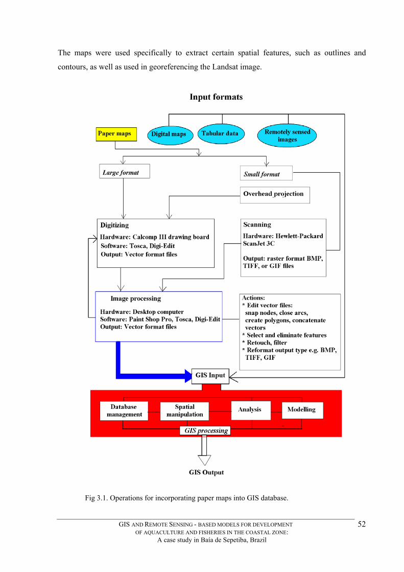
The maps were used specifically to extract certain spatial features, such as outlines and

contours, as well as used in georeferencing the Landsat image.

Fig 3.1. Operations for incorporating paper maps into GIS database.



52

The key settings configuration for the digitising board was set to that of the factory default for

‘CalComp 2000 ASCI’. To digitise, a Calcomp 6-button model puck was used.

The puck’s button functions were reassigned for use with both Tosca and Digi-Edit digitising

software, so that buttons 0, 1, 2 and 3 corresponded to button functions digitise, snap, end

(finish) and toggle respectively. Digitising software included TOSCA, and Tsoft DIGI-EDIT

for Windows version 1.050. At the beginning of this study, the paper maps used were

digitised using the DOS-based TOSCA software (Jeffrey F. Jones, IDRISI Project). Later,

other maps were digitised using an improved version of TOSCA marketed as DIGI-EDIT 1.0

for Windows. In the course of this project, several paper maps were consulted, from which it

was necessary to extract selected information to complement the GIS database. Point, line and

polygon information are exemplified as point location of oyster or mussel banks along the

coastline (points), road network (lines), and urban or conservation areas (polygons).

Some digitising was also achieved using the mouse and on-screen tools available in image

processing software such as PaintShop Pro 5, and in IDRISI, the GIS software used in this

study. 3.6 - Scanned images

Much useful and relevant information for this study was available only as printed images such

as choropleth maps illustrating government agency reports or in published papers, many of

which were less than A4 size paper. Selected images were scanned on a Hewlett-Packard

flatbed scanner (model ScanJet 3C; Descan II v 2.8), and saved as bitmap images.

Choropleths were typically scanned at 150 dpi resolution. Scanning images is a very efficient

way of incorporating information as raster layers into a GIS. Vector layers can be derived

from rasterized scanned images by digitising in image processing software.

3.7 - Maps used

A list of maps used is presented in Table 3.3. The map publishers included the Brazilian

Naval Hydrographic Office, the Army Cartographic Service and the Brazilian Institute of

Geography and Statistics. Other maps, including choropleth maps, were obtained from studies

and reports as A-4 size. These were scanned, saved as bitmap images and later incorporated

into the GIS database by use of the import facility of IDRISI (Fig 3.2).



53

Fig 3.2. Spatial manipulations of scanned or digital information to incorporate into raster-based layers in a GIS.



54

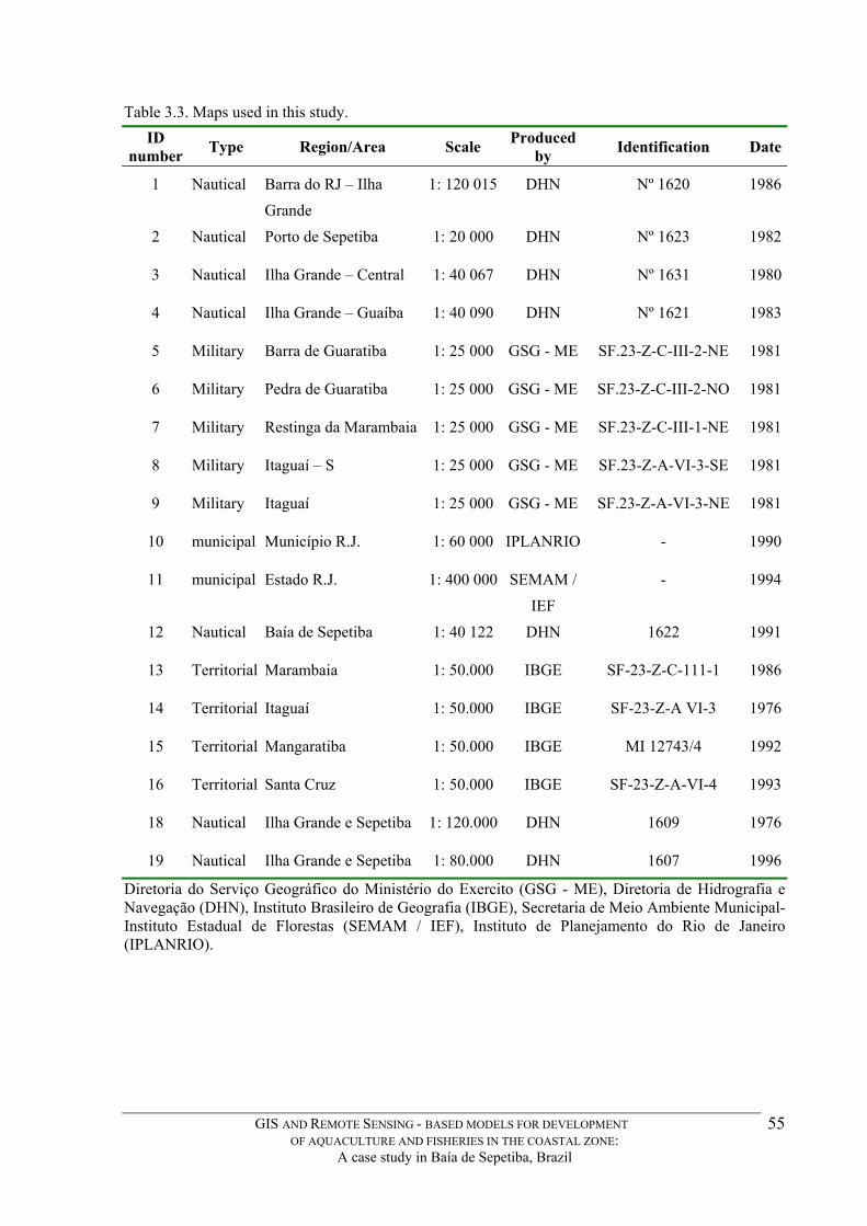
Table 3.3. Maps used in this study. ID

number Type Region/Area Scale Produced by Identification Date

1 Nautical Barra do RJ – Ilha Grande

1: 120 015 DHN Nº 1620 1986

2 Nautical Porto de Sepetiba 1: 20 000 DHN Nº 1623 1982

3 Nautical Ilha Grande – Central 1: 40 067 DHN Nº 1631 1980

4 Nautical Ilha Grande – Guaíba 1: 40 090 DHN Nº 1621 1983

5 Military Barra de Guaratiba 1: 25 000 GSG - ME SF.23-Z-C-III-2-NE 1981

6 Military Pedra de Guaratiba 1: 25 000 GSG - ME SF.23-Z-C-III-2-NO 1981

7 Military Restinga da Marambaia 1: 25 000 GSG - ME SF.23-Z-C-III-1-NE 1981

8 Military Itaguaí – S 1: 25 000 GSG - ME SF.23-Z-A-VI-3-SE 1981

9 Military Itaguaí 1: 25 000 GSG - ME SF.23-Z-A-VI-3-NE 1981

10 municipal Município R.J. 1: 60 000 IPLANRIO - 1990

11 municipal Estado R.J. 1: 400 000 SEMAM / IEF

- 1994

12 Nautical Baía de Sepetiba 1: 40 122 DHN 1622 1991

13 Territorial Marambaia 1: 50.000 IBGE SF-23-Z-C-111-1 1986

14 Territorial Itaguaí 1: 50.000 IBGE SF-23-Z-A VI-3 1976

15 Territorial Mangaratiba 1: 50.000 IBGE MI 12743/4 1992

16 Territorial Santa Cruz 1: 50.000 IBGE SF-23-Z-A-VI-4 1993

18 Nautical Ilha Grande e Sepetiba 1: 120.000 DHN 1609 1976

19 Nautical Ilha Grande e Sepetiba 1: 80.000 DHN 1607 1996

Diretoria do Serviço Geográfico do Ministério do Exercito (GSG - ME), Diretoria de Hidrografia e Navegação (DHN), Instituto Brasileiro de Geografia (IBGE), Secretaria de Meio Ambiente Municipal- Instituto Estadual de Florestas (SEMAM / IEF), Instituto de Planejamento do Rio de Janeiro (IPLANRIO).



55

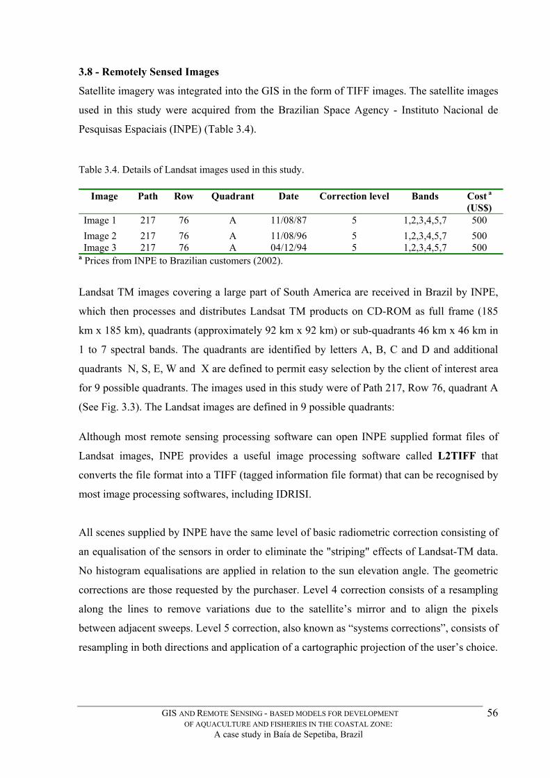
3.8 - Remotely Sensed Images

Satellite imagery was integrated into the GIS in the form of TIFF images. The satellite images

used in this study were acquired from the Brazilian Space Agency - Instituto Nacional de

Pesquisas Espaciais (INPE) (Table 3.4).

Table 3.4. Details of Landsat images used in this study.

Image Path Row Quadrant Date Correction level Bands Cost a (US$)

Image 1 217 76 A 11/08/87 5 1,2,3,4,5,7 500 Image 2 217 76 A 11/08/96 5 1,2,3,4,5,7 500 Image 3 217 76 A 04/12/94 5 1,2,3,4,5,7 500

a Prices from INPE to Brazilian customers (2002).

Landsat TM images covering a large part of South America are received in Brazil by INPE,

which then processes and distributes Landsat TM products on CD-ROM as full frame (185

km x 185 km), quadrants (approximately 92 km x 92 km) or sub-quadrants 46 km x 46 km in

1 to 7 spectral bands. The quadrants are identified by letters A, B, C and D and additional

quadrants N, S, E, W and X are defined to permit easy selection by the client of interest area

for 9 possible quadrants. The images used in this study were of Path 217, Row 76, quadrant A

(See Fig. 3.3). The Landsat images are defined in 9 possible quadrants: Although most remote sensing processing software can open INPE supplied format files of

Landsat images, INPE provides a useful image processing software called L2TIFF that

converts the file format into a TIFF (tagged information file format) that can be recognised by

most image processing softwares, including IDRISI.

All scenes supplied by INPE have the same level of basic radiometric correction consisting of

an equalisation of the sensors in order to eliminate the "striping" effects of Landsat-TM data.

No histogram equalisations are applied in relation to the sun elevation angle. The geometric

corrections are those requested by the purchaser. Level 4 correction consists of a resampling

along the lines to remove variations due to the satellite’s mirror and to align the pixels

between adjacent sweeps. Level 5 correction, also known as “systems corrections”, consists of

resampling in both directions and application of a cartographic projection of the user’s choice.



56

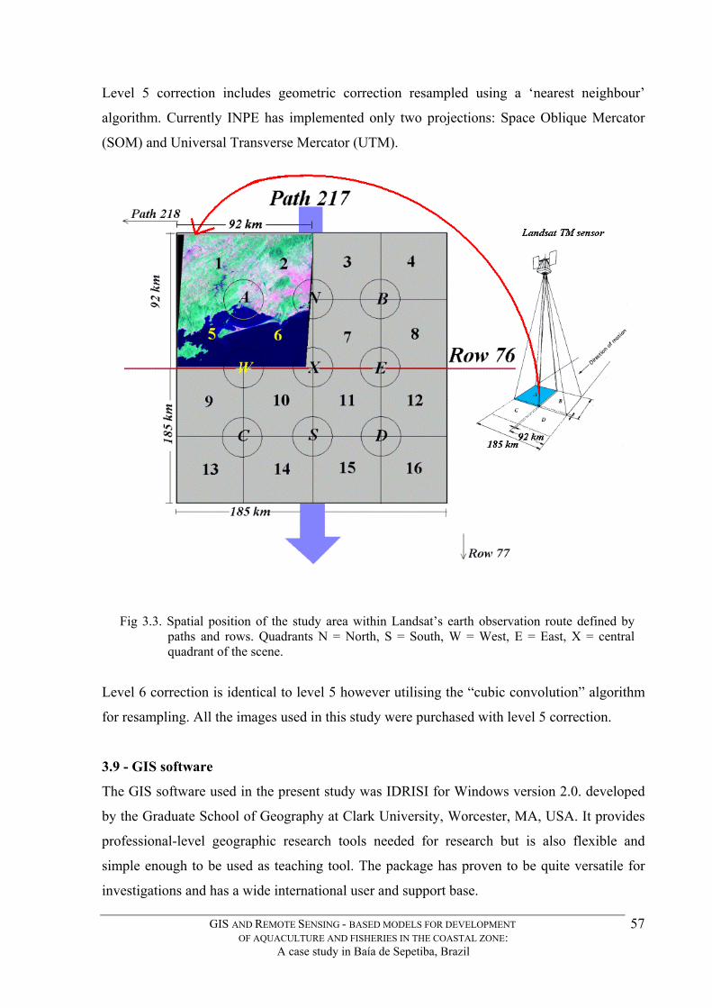
Level 5 correction includes geometric correction resampled using a ‘nearest neighbour’

algorithm. Currently INPE has implemented only two projections: Space Oblique Mercator

(SOM) and Universal Transverse Mercator (UTM).

Fig 3.3. Spatial position of the study area within Landsat’s earth observation route defined by

paths and rows. Quadrants N = North, S = South, W = West, E = East, X = central quadrant of the scene.

Level 6 correction is identical to level 5 however utilising the “cubic convolution” algorithm

for resampling. All the images used in this study were purchased with level 5 correction.

3.9 - GIS software

The GIS software used in the present study was IDRISI for Windows version 2.0. developed

by the Graduate School of Geography at Clark University, Worcester, MA, USA. It provides

professional-level geographic research tools needed for research but is also flexible and

simple enough to be used as teaching tool. The package has proven to be quite versatile for

investigations and has a wide international user and support base.



57

The software used in this study contains a collection of over 150 program modules that

provide facilities for input, display and analysis of geographic data. In this thesis, these

modules will be indicated in bold and capital letters.

Traditionally, IDRISI has been attractive because of its raster analytical functionality,

covering GIS and remote sensing needs from basic database query, to more importantly,

spatial modelling, and image enhancement and classification (Eastman, 1997). IDRISI’s

analytical modules were periodically cleaned of ‘bugs’ and made available to users as

downloads from their website (http://www.clarklabs.org). Currently, the company does not

support updates for version 2.0.

IDRISI has import tools for a range of file formats ranging from desktop publishing, raw

raster image files and other GIS software packages including ARC-INFO, MAP-INFO,

ERDAS, ATLAS-GIS GRASS, and SURFER.

GIS technology tends to be expensive in terms of software, hardware and training. However,

the IDRISI project’s philosophy has been to adopt the notion of democratisation of

technology and considers that tools such as GIS should not be reserved solely for those with

large budgets, but should be available to all who have a need for them. The IDRISI project is

essentially a non-profit organisation committed to maintaining the viability of the organisation

and the continued improvement of the software. Currently the latest version of the product,

IDRISI KILIMANJARO is relatively affordable at US$ 600 for a single academic license

(IDRISI, 2003).

3.10 - Image Manipulation

Paint Shop Pro 5, a raster-format image editing software, proved to be a relatively workable

tool to learn. With practise, images were manipulated and processed prior to or during the

modelling phases carried out in the ‘full’ GIS environment. Paint Shop Pro 5 allows for

extensive image editing with more ease than possible in the 16 bit version of IDRISI for

Windows 2.0. Pre-treatment or editing of images allowed for the elimination of features of no

interest while retaining others (see Fig 3.2 for example) and although this is also possible in

IDRISI, it is more cumbersome.



58

http://www.clarklabs.org/

Specifically, on-screen digitisation in IDRISI has limitations related to the buffer capacity for

the vector file being worked upon, often leading to the abrupt termination of the program due

to insufficient available memory problems, resulting in total loss of files in the digitisation

process. Paint Shop Pro 5 also allows direct scanning of images, editing, and saving in a wide

variety of digital formats, including as bitmaps or tagged information file format (TIFF).

To make use of image files edited in Paint Shop Pro 5, a process of resampling the imported

images in the IDRISI environment is necessary (See Fig 3.2). Once the bitmap image has

been imported and saved as an IDRISI image file, it must be resampled to match the spatial

definitions of the base image which is being worked upon. To accomplish this, an ASCII file

containg a number of corresponding co-ordinate pairs must be created and saved as a

‘correspondence file’ in IDRISI.

3.11 - Cutting a window of the study area

The Landsat file supplied by INPE covers the upper left hand quarter of the full scene for path

217 row 76 (Fig 3.3). As the focus of this study concerns the coastal area of Sepetiba Bay, as

well as nearby adjacent coastal areas, a selection was made based on the fact that most water

quality data available for the area coincides with the area spanned by admiralty chart number

1622 published by the Brazilian Naval Hydrogaphic Office DHN (see Fig 3.2). It could be

argued that a study of this nature should include the entire hydrographic basin relative to

Sepetiba Bay. However, at the start of this study there was insufficient information to show

the boundaries of this hydrographic basin, which is beyond the limits of this quadrant and

would possibly involve the purchase of a second partial scene, that of path 217 row 75

quadrant C. Usually Landsat images can be displaced up to 10% north or south without extra

cost to the client. Considering that most of the processes which directly affect fisheries and

potential aquaculture development are within close range of the coastline, the subset image

was considered appropriate.

Once this subset window of the sudy area was defined, it was extracted using the WINDOW

option of the ‘Reformat’ menu in IDRISI. This option offers a ‘batch window’, cutting option

that will process multiple images (such as individual bands) for the same specified area, as

determined by column and row, or if the image is georeferenced, by geographical position.



59

The area windowed and cut for study covered columns 845 to 2,810, and rows 1,268 to 2,609

of the original Landsat image (Fig 3.2).

3.12 - Georeferencing

To georeference is to establish the relationship between page co-ordinates on a planar map

and known real-world co-ordinates. (AGI, 1999).

In IDRISI, the geographic files are assumed to be stored according to a grid reference system

where grid north is aligned with the edges of the raster image or vector file. Documentation

files for all images contain information about the reference system used by that file when

referring to geographic locations. The particulars of the reference system (e.g., projection,

datum and origin) are contained in a reference system parameter file. Each grid reference

system must have a reference system parameter file. The only exception is the system

identified by the keyword plane. Any image or vector file with a plane coordinate referencing

system is understood to use an arbitrary plane system for which geodetic and projection

parameters are unknown, and for which a reference system parameter file is not provided

(Eastman, 1997)

3.12.1 - Georeferencing the satellite image.

Although the INPE Landsat TM image was furnished as georeferenced, the import process

using TIFF format conversion did not retain co-ordinate information in latitude and longitude.

Therefore when this image was imported into IDRISI its reference system was re-set to plane,

and had to be subsequently georegistered.

Georegistration is also known as ‘rubber sheeting’ or ‘resampling’. It is the process of

stretching and warping an image to fit a particular grid reference system. Resampling is

accomplished by identifying a series of x,y coordinates of two pairs of points that represent

the same place within both a new and an old or previous coordinate system (Eastman 1997).

The x,y, co-ordinate pairs are entered directly in the EDIT facility of IDRISI, or alternately,

entered in a spread sheet application such as Microsoft Excel or any text editor. The list is

then saved as a text or MS-DOS format file, which can be easily imported into IDRISI.



60

Georeferencing the satellite image requires that clear ground control points be known from a

source such as a map, or field coordinates of locations derived with a Global Positioning

System (GPS).

In this study, as the satellite image imported into the GIS was non-georeferenced, a list of

over 150 point co-ordinates, which were clearly identifiable both on the Landsat satellite

image of Dec 04, 1994 image as well as on admiralty chart DHN 1622, was generated. These

points were typically small islands, headlands, railroad track and vehicle road crossings, i.e

points which are unlikely to change over time.

For all these points, their co-ordinates in the Landsat image was noted along with their

corresponding co-ordinates in degree, minute and decimal minute from the admiralty chart

DHN 1622. (Appendix 1).

As this admiralty chart was used for many notations and references to field data, several

features were digitised. This digitisation was one of the first tasks of the laboratory-based

operations, and was done using TOSCA digitisation software. The co-ordinate pairs for the

resulting vector file which were georeferenced to the Landsat image are found in Appendix 2.

The visual identification of the ground control points on the Landsat TM image was effected

on a false colour (RGB) composite image of bands 7,4,2 saturated at 2.5% generated in

IDRISI using the module COMPOSIT. This band combination provides good contrast

between reflectances coming from water bodies, urban structures and vegetation, showing

urban areas in tones of magenta, vegetation showing in familiar green tones and water bodies

in dark colours. Contrast between soil and water interfaces are marked which facilitates

identification of road and river crossings, which are commonly used georeferencing sites.

This admiralty chart and all other digitised paper maps were then georegistered to the Landsat

image using the the module RESAMPLE. ‘RESAMPLE’ registers the data in one grid

system to a different grid system covering the same area. The process uses polynomial

equations to establish a rubber sheet transformation, as if one grid were placed on rubber and

warped to make it correspond to the other.



61

The process involves constructing and development of a set of polynomial equations to

describe the spatial mapping of data from the old grid to the new one. The new grid is then

filled with data values by resampling the old grid and estimating, if necessary, the new value

(Eastman, 1992).

Before georeferencing resampling can be done, the windowed-out part of the full Landsat TM

image has to have its IDRISI ‘document file’ altered so that its minimum x and y co-ordinates

are set to zero. The maximum x, and y then become the number of rows and columns for the

satellite image spanned, in this case 1966 columns and 1342 rows.

The type of resampling used was the ‘linear’ with ‘nearest neighbour’. In general, one should

use the lowest order of polynomial that provides a reasonable solution since the effect of poor

control point specification gets dramatically worse as the order of equation used increases. It

is also, necessary to ensure that there are an adequate number of control points for the order

chosen. Linear sampling requires a minimum of 3, quadratic sampling requires 6 and cubic

sampling requires 10.

In practice however, at least twice the minimum are required for a reasonable fit (Eastman,

1992). A peculiarity of the specific ‘windowed section’ of the satellite image used in this

study was that a large area (48.4%) is covered with open waters, where ground control points

are very scarce or non-existent.

In coastal areas sand spits or mangrove islands represent important sites but are unsuitable as

good ground control points for georeferencing due to their mobility.

During the first resampling trials, improper correlations resulted in grossly distorted

resampled images. A technique was thus developed which in essence, is similar to that used in

nautical navigation – triangulation (Fig 3.4) and consisted of drawing several reference lines

(as vector files overlying the raster satellite image), from well established reference points.

One peculiarity of the satellite image window studied is that it includes a small coastal island

out at sea, Lage da Marambaia, which facilitated extending reference lines out to noteworthy

points on the coastline.



62

Fig 3.4. Steps followed for georeferencing the cut-out window of the study area.

Other auxiliary lines were also developed from other points in order to produce lines with

reference points on the intersection of lines over open water. Thus, new ‘virtual’ control

points were created for the correspondence file over the otherwise featureless open water

stretches. Corresponding lines were also drawn on admiralty chart DHN 1622 from the same

control points as those used on the Landsat TM image. The intersection of the lines provided

corresponding points with known latitude-longitude co-ordinates.



63

This process was found to be adequate for the georeferencing proposed. To use the longitude,

latitude, co-ordinates in the IDRISI correspondence file, they were converted to decimal

format by using the formula:

Decimal degree = Longitude or Latitude degrees + (minutes + decimal minutes/60)

As all field data points recorded on the GPS were in degree, minute and decimal minute

format, they had to be converted to degree and decimal degree format for georeferencing by

spreadsheet. An example is given in Fig 3.4. Due to IDRISI’s georeferencing system,

longitudes West of Greenwich, and South of the equator must be specified as negative

numbers. The final co-ordinate value has to be specified in scientific notation for entry into

IDRISI’s correspondence file.

All field points were thus converted into decimal degree format in order to match the GIS

environment. The resampling process is sumarised in Fig 3.5. The accuracy of the resampling

is verified by its Root Mean Square (RMS) error, the distance between the input (source)

location of a ground control point and the retransformed location for the same GCP (ERDAS,

1997). In other words, it is the difference between the desired output co-ordinate for a GCP

and the actual output co-ordinate for the same point, when the point is transformed with the

transformation matrix. RMS error is calculated with a distance equation:

22error RMS ) y (y ) x(x irir +=

where xi and yi are the input source co-ordinates and xr and yr are the retransformed co-

ordinates.

The RMS error is expressed as a distance in the source co-ordinate system. In this case the

units are pixels. The process and results of the resampling operation are illustrated in Figs. 3.5

and 3.6. The overall RMS error achieved with the image rectification in this project was

3.078, which means that any pixel could be in error by as much as 90 m. When rectifying

Landsat TM data, ERDAS (1997) recommends an of +- 30 m, and therefore the RMS error

should not exceed 0.50 In the present study, the RMS error over the area was judged to be

sufficient for modelling purposes.



64

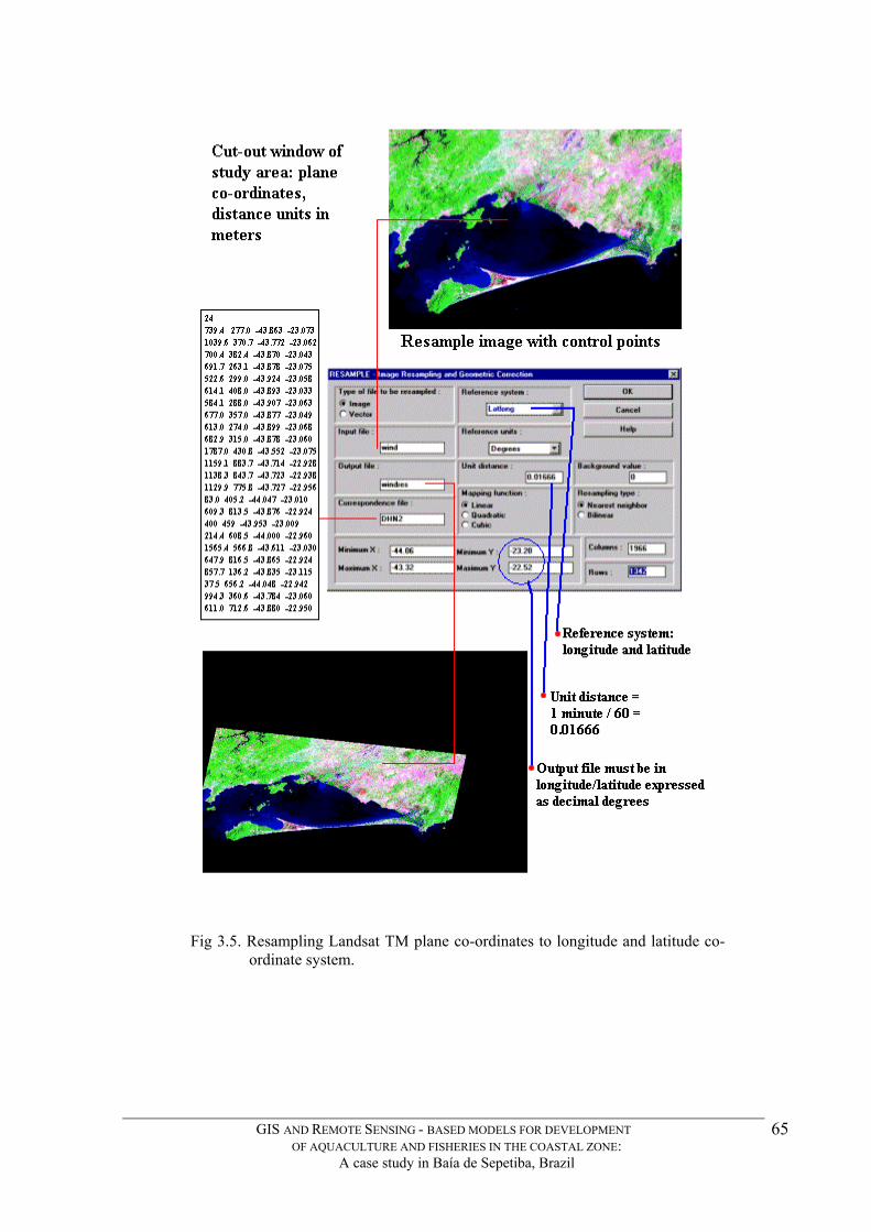
Fig 3.5. Resampling Landsat TM plane co-ordinates to longitude and latitude co-

ordinate system.



65

Resample: Summary of Transformation

Computed polynomial surface : Linear (based on 24 control points)

Coefficient X Y b0 135639.3499915736250000 107742.2455669621050000 b1 3373.2237179039660200 534.3147077957235210 b2 -565.9885112465267410 3641.9123988303115300

Note: Figures are carried internally to 20 significant figures. Formula shown is the back transformation (new to old).

Control points used in the transformation :

Old X Old Y New X New Y Residual 739.400000 277.000000 43.863000 23.073000 1.432948 1039.600000 370.700000 43.772000 23.062000 6.263914 700.400000 382.400000 43.870000 23.043000 2.562867 691.700000 263.100000 43.878000 23.075000 3.621772 522.600000 299.000000 43.924000 23.058000 2.197472 614.100000 408.000000 43.893000 23.033000 2.705581 584.100000 288.000000 43.907000 23.063000 0.836825 677.000000 357.000000 43.877000 23.049000 1.587408 613.000000 274.000000 43.899000 23.068000 1.600622 682.900000 315.000000 43.878000 23.060000 2.166897 1787.000000 430.800000 43.552000 23.075000 4.284881 1159.100000 883.700000 43.714000 22.928000 0.287632 1138.300000 843.700000 43.723000 22.938000 4.047621 1129.900000 775.800000 43.727000 22.956000 1.841301 83.000000 405.200000 44.047000 23.010000 1.798835 609.300000 813.500000 43.876000 22.924000 2.375709 400.000000 459.000000 43.953000 23.009000 2.078040 214.400000 608.500000 44.000000 22.960000 5.871613 1565.400000 566.800000 43.611000 23.030000 1.014931 647.900000 816.500000 43.865000 22.924000 0.879488 857.700000 136.200000 43.835000 23.115000 1.743148 37.500000 656.200000 44.048000 22.942000 3.722025 994.300000 360.600000 43.784000 23.060000 5.879077 611.000000 712.600000 43.880000 22.950000 2.153960

Overall RMS = 3.078090

Fig 3.6. Results of the RESAMPLE operation carried out to georeference windowed area of Landsat

image.



66

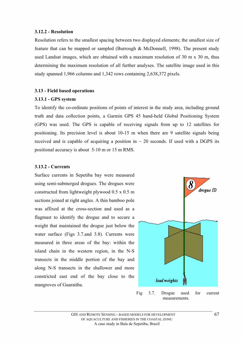
3.12.2 - Resolution

Resolution refers to the smallest spacing between two displayed elements; the smallest size of

feature that can be mapped or sampled (Burrough & McDonnell, 1998). The present study

used Landsat images, which are obtained with a maximum resolution of 30 m x 30 m, thus

determining the maximum resolution of all further analyses. The satellite image used in this

study spanned 1,966 columns and 1,342 rows containing 2,638,372 pixels.

3.13 - Field based operations

3.13.1 - GPS system

To identify the co-ordinate positions of points of interest in the study area, including ground

truth and data collection points, a Garmin GPS 45 hand-held Global Positioning System

(GPS) was used. The GPS is capable of receiving signals from up to 12 satellites for

positioning. Its precision level is about 10-15 m when there are 9 satellite signals being

received and is capable of acquiring a position in ~ 20 seconds. If used with a DGPS its

positional accuracy is about 5-10 m or 15 m RMS.

3.13.2 - Currents

Surface currents in Sepetiba bay were measured

using semi-submerged drogues. The drogues were

constructed from lightweight plywood 0.5 x 0.5 m

sections joined at right angles. A thin bamboo pole

was affixed at the cross-section and used as a

flagmast to identify the drogue and to secure a

weight that maintained the drogue just below the

water surface (Figs 3.7.and 3.8). Currents were

measured in three areas of the bay: within the

island chain in the western region, in the N-S

transects in the middle portion of the bay and

along N-S transects in the shallower and more

constricted east end of the bay close to the

mangroves of Guaratiba.

Fig 3.7. Drogue used for current measurements.



67

Drogues were sequentially placed in the water from a

speedboat, their initial geographical position in

longitude and latitude and time being recorded

(Appendix 3). As many as 8 drogues were

sequentially dropped along a transect. As the last

drogue of the series was launched, the speedboat

returned along the transect line towards the first

drogue position, recording the time and position of

the intermediary drogues. The speedboat then

returned directly to the last drogue dropped and began

its final return trip collecting position and time

information. The areas surveyed are identified in Fig.

3.9.

Fig 3.8. Launching drogues in Sepetiba.

3.13.3 - Salinity and temperature

Salinity and temperature are important variables that vary considerably in space and time.

Although it was not possible to do extensive surveying of these variables during this research,

fields measurements were made in order to provide a range of values for consideration during

the modeling process. Figure 3.9 shows the distribution of points for which salinity,

temperature and depth measurements were taken on several field trips to the bay.

These measurements were taken at the same time as other data collecting activities were being

undertaken such as measuring of current speeds, bottom sediment sampling, and site

reconaissance trips. Salinity was measured using a Biofauna Aquamarine salinity

refractometer, with a scale of 1- 100‰ with 0.1‰ precision, temperature with a lab

thermometer (± 0.1 ºC) and depth was recorded from the on board echosounder, a 2D

Hummingbird model 00, equipped with single beam transducer 128V x 64H, super-twist LCD

display, depth capability of 200m. Appendix 4 show geographic position, temperature,

salinity and depth values recorded during the field expeditions.



68

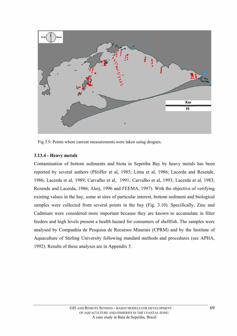
Fig 3.9. Points where current measurements were taken using drogues.

3.13.4 - Heavy metals

Contamination of bottom sediments and biota in Sepetiba Bay by heavy metals has been

reported by several authors (Pfeiffer et al, 1985; Lima et al, 1986; Lacerda and Resende,

1986; Lacerda et al, 1989; Carvalho et al, 1991; Carvalho et al, 1993; Lacerda et al, 1983;

Rezende and Lacerda, 1986; Alerj, 1996 and FEEMA, 1997). With the objective of verifying

existing values in the bay, some at sites of particular interest, bottom sediment and biological

samples were collected from several points in the bay (Fig. 3.10). Specifically, Zinc and

Cadmium were considered more important because they are known to accumulate in filter

feeders and high levels present a health hazard for consumers of shellfish. The samples were

analysed by Companhia de Pesquisa de Recursos Minerais (CPRM) and by the Institute of

Aquaculture of Stirling University following standard methods and procedures (see APHA,

1992). Results of these analyses are in Appendix 5.



69

Fig 3.10. Distribution of water quality measurement points.

3.13.5 - Land use verification (Ground truthing)

Observations of characteristic vegetation, ground cover, patterns of land use, positions of

crossroads, industrial sites and other points of interest were recorded using GPS during field

trips over the landside of the study area (Appendix 7). This data was important because it

provided information for manual georeferencing of the landsat image with co-ordinates other

than those collected from the paper maps utilised as well as provided a better feel for the

actual land cover in relation to the 742 (RGB) colour composite of the Landsat image. These

ground control points are illustrated in Fig. 3.11.



70

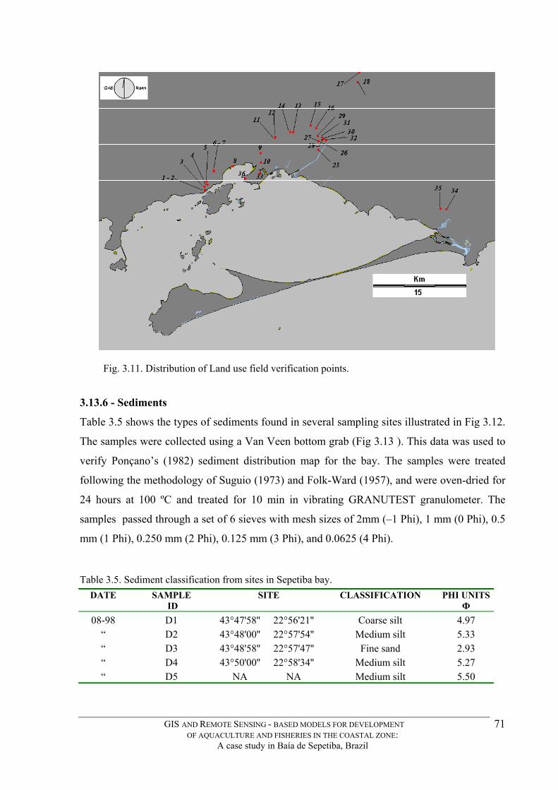
Fig. 3.11. Distribution of Land use field verification points.

3.13.6 - Sediments

Table 3.5 shows the types of sediments found in several sampling sites illustrated in Fig 3.12.

The samples were collected using a Van Veen bottom grab (Fig 3.13 ). This data was used to

verify Ponçano’s (1982) sediment distribution map for the bay. The samples were treated

following the methodology of Suguio (1973) and Folk-Ward (1957), and were oven-dried for

24 hours at 100 ºC and treated for 10 min in vibrating GRANUTEST granulometer. The

samples passed through a set of 6 sieves with mesh sizes of 2mm (–1 Phi), 1 mm (0 Phi), 0.5

mm (1 Phi), 0.250 mm (2 Phi), 0.125 mm (3 Phi), and 0.0625 (4 Phi).

Table 3.5. Sediment classification from sites in Sepetiba bay. DATE SAMPLE

ID SITE CLASSIFICATION PHI UNITS

Ф 08-98 D1 43°47'58'' 22°56'21'' Coarse silt 4.97

“ D2 43°48'00'' 22°57'54'' Medium silt 5.33 “ D3 43°48'58'' 22°57'47'' Fine sand 2.93 “ D4 43°50'00'' 22°58'34'' Medium silt 5.27 “ D5 NA NA Medium silt 5.50



71

“ D6 NA NA Coarse silt 4.40 “ D9 43°46'24'' 22°58'48'' Coarse silt 4.27

01-97 C1 43.41.919 23.01.909 Fine sand 2.06 “ C2 43.36.980 23.01.128 Coarse silt 4.71 “ C3 43.38.008 23.01.484 Medium silt 5.09 “ C4 43.37.399 23.01.700 Coarse silt 4.98 “ C5 43.54.927 23.01.854 Very fine sand 3.43 “ C6 43.39.366 23.01.931 Coarse silt 4.54 “ C7 43.43.047 23.02.557 Coarse silt 4.42 “ C9 43.54.877 22.57.302 Fine sand 2.11 “ C10 43.54.591 23.00.329 Very fine sand 3.37 “ C11 43.57.005 23.00.048 Very fine sand 3.23 “ C14 43.55.209 22.59.825 Coarse silt 4.37

07-96 B1 43.49.807 22.57.611 Medium silt 5.33 “ B2 43.50.501 22.56.428 Medium silt 5.50 “ B3 43.49.655 22.59.373 Coarse silt 4.10 “ B4 43.49.476 23.00.838 Very fine sand 3.80

03-96 A1 43.52.420 22.56.954 Medium silt 5.50 “ A2 43.53.849 22.58.627 Medium sand 1.47 “ A3 43.54.633 22.59.384 Very fine sand 3.37 “ A4 43.56.161 23.00.741 Very fine sand 3.07 “ A5 43.56.730 23.00.090 Medium sand 1.37 “ A6 43.56.102 23.00.659 Medium sand 1.33 “ A7 43.51.720 22.57.412 Very fine sand 3.07 “ A10 43.53.952 22.57.539 Coarse silt 4.57 “ A11 43.48.844 22.55.599 Medium silt 5.83 “ A13 43.51.053 22.55.922 Medium silt 5.63 “ A14 43.50.405 22.56.216 Medium silt 5.90 “ A15 43.49.876 22.56.089 Coarse silt 4.17 “ A16 43.48.799 22.56.726 Medium silt 5.10 “ A17 43.47.802 22.55.982 Very fine sand 3.73 “ A18 43.47.872 22.56.863 Coarse silt 4.50 “ A21 43.43.300 22.58.469 Medium silt 5.33



72

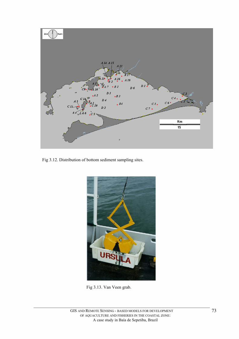
Fig 3.12. Distribution of bottom sediment sampling sites.

Fig 3.13. Van Veen grab.



73

3.13.7 - Mussel distribution

Although mussel growth in the bay is possible, it is limited in many places by a lack of

substrate for the mussel larvae to settle. In other places salinity is too low for successful spat

fixation. As mussel aquaculture is not currently practised in Sepetiba bay, ground truth for

this factor was based on local knowledge of the bay’s natural mussel banks present on

submerged rocks and rocky coastlines and also the sites where the fish traps are installed, as

they have mussel growing on them. Other sites were investigated by consulting with a local

expert who had 10 years of fishing and diving experience in the bay. Figure 3.14 shows the 10

sites identified by the expert. In his experience, mussel bank sites were more abundant in the

past. In an attempt to confirm this, a culture trial was started with 10 mussel starter ropes,

measuring 1m in length and 7 cm. in diameter. The young mussels were purchased from the

Jurujuba fishing coop in Niterói and placed in Sepetiba waters on April 1996. The ropes were

transported across Guanabara Bay in a 15 minute trip, from where they were transferred to a

pick-up truck in Rio, arriving in Itacuruçá port in 2.5 hours. With the aid of a 50HP engine

speedboat, the mussel ropes were transported to, and installed at the 10 sites listed in table 3.6

within 4 hours of arrival. At the time of installation a sample of the bottom sediment was

taken with a Van-Veen grab, and visually assessed for quality (Table 3.6). No lab analysis

was undertaken.

The expert’s rationale for siting the experimental mussel culture installation included shelter

from wind, proximity to the shore, distance from industrial pollution sources, distance from

navigational areas, closeness to own residence (site 10), and subjective knowledge of water

quality aspects, the most important of which were salinity and temperature.

The mussel ropes were visually inspected by diving once a month for the first three months.

The mussels were checked for survival during this period, but growth was not measured.



74

Fig 3.14. Experimental mussel culture installation sites. 1. Bóia Vermelha 2. Laje - Praia do Leste 3. Ilha do Martins 4. Boa Vista 5. Ilha Jurubaíba 6. Ilha da Bala 7. Ilha do Bernardo 8. Ilha Bonitinha 9. Ilha do Bicho Grande 10. Praia Grande.

Ropes 1 and 10 had heavy infestation of ascidians, which apparently stifled mussel growth.

After 3 months, most of the experimental mussel ropes had disappeared. It is believed that

they were taken away by local residents, mostly interested in keeping the anchor which held

the rope to the buoy. The experiment was discontinued.



75

Table 3.6. Sites selected for mussel culture trial.

Mussel rope id Mooring site Longitude Latitude Sediment type

1 Bóia Vermelha 43.51.400 22.55.628 Mud 2 Laje - Praia do Leste 43.52.038 22.55.756 Gravel 3 Ilha do Martins 43.51.788 22.56.830 Gravel 4 Boa Vista 43.54.536 22.57.394 Gravel 5 Ilha Jurubaíba 43.57.052 22.57.512 Gravel 6 Ilha da Bala 43.56.759 23.00.236 Gravel 7 Ilha do Bernardo 43.57.265 23.01.354 Rocky/Gravel 8 Ilha Bonitinha 43.54.706 22.59.774 Gravel 9 Ilha do Bicho Grande 43.55.330 22.59.107 Rocky/Gravel

10 Praia Grande 43.54.427 22.56.798 Mud

Considering that the artisanal fish traps managed by the fishermen of Pedra de Guaratiba are

good indicators of potential mussel spat collection and on-growing areas, the relative position

of 42 traps and their state of repair was recorded on 30.01.97 as can be seen on Fig 3.15 and

Table 3.7.

Fig. 3.15. Distribution of 42 fish traps along the Marambaia island.



76

Table 3.7. Fish traps (Cercadas) position and usage status in Sepetiba Bay.

CO-ORDINATES NUMBER OF TRAPS

DEPTH (M)

OBS.

Longitude W Latitude S 43.38.013 23.01.554 2 1.8 in use 43.37.965 23.01.473 2 3.3 in use 43.38.200 23.01.498 2 3.6 in use 43.38.452 23.01.538 1 - broken 43.38.593 23.01.563 1 - new 43.38.704 23.01.641 2 2.7 in use 43.38.765 23.01.587 1 - in use 43.39.141 23.01.750 2 - in use 43.39.180 23.01.613 1 1.8 in use 43.39.366 23.01.931 2 - one old, one new 43.39.439 23.01.650 2 3.0 In use 43.39.548 23.01.725 1 - Good shape 43.39.814 23.01.821 1 3.0 In use 43.40.011 23.01.800 1 3.0 In use 43.40.065 23.01.714 1 3.0 In use 43.40.128 23.01.762 1 - In use 43.40.298 23.01.735 1 - In use 43.40.594 23.01.876 1 3.3 In use 43.40.858 23.01.854 1 - In use 43.40.936 23.01.916 1 3.3 In use 43.41.362 23.01.886 2 3.6 both broken 43..41.594 23.01.964 1 - Good shape 43.41.604 23.01.921 2 3.9 New, side by side 43.41.695 23.02.040 1 3.3 In use 43.41.803 23.01.980 2 3.96 1 new, 1 broken 43.42.345 23.02.022 1 - In use 43.42.419 23.02.128 1 3.96 In use 43.42.651 23.02.257 1 - In use 43.42.730 23.02.320 1 - New 43.42.823 23.02.438 2 - Broken 43.42.994 23.02.527 1 4.3 New

Total 42 - Average depth - 3.2 -



77

CHAPTER 4.

DATABASE DEVELOPMENT

4.1 -Introduction

Aquaculture development in the coastal zone depends on the natural resources available and

conditions of the physical environment. Selected fisheries resources present in Sepetiba are

briefly reviewed in order to identify best candidate species. Their growth depends on several

environmental parameters, which were mapped, reclassified and scored for suitability in the

GIS.

4.2 - Culture species selection

Bivalve molluscs represent the most important aquaculture candidates. Sepetiba has exploited

populations of brown mussels (Perna perna), mangrove oysters (Crassostrea rhizophorae),

venerid clams (Anomalocardia brasiliana) and the mangrove mussel (Mytella falcata). These

species grow in the bay and natural seed sources for these can be found in the area. Sepetiba

bay also is an important feeding and reproduction environment for many fish species, some of

which have culture potential, including groupers, mullets, flatfish and snook. So far, bivalve

molluscs are the only group cultured in the bay. Their culture requires low investment and

running costs make it a good option for local entrepreneurs/fishermen. This is in line with the

Brazilian Ministry of Agriculture and Fisheries which in its development strategies for the

period 2000-2001 has proposed action lines and credit for the development of 'aquaculture

production chains' which include bivalve molluscs, specifically mussels and oysters and the

exotic white shrimp Litopenaeus vannamei. These species were selected as the best initial

options for aquaculture development (Proença, 2002). In this study, site selection modelling

for the brown mussel Perna perna, the native mangrove oyster C. rhizophorae, and the exotic

white shrimp Penaeus vannamei was developed.

Mussel and oyster culture have long attracted the attention of aquaculture and fisheries

development institutions in Rio de Janeiro. Moreira (1985) developed a mariculture manual

for Perna perna and Crassostrea gigas for the Cabo Frio region. Magalhães and Ferreira

(1997) have recently summarised the current technical practices commonly used for the

culture brown mussels in Brazil.



78

The exotic white shrimp Litopenaeus vannamei is now cultured semi-intensively to

intensively in most coastal states of Brazil. It is a hardy species, tolerant of a wide range of

environmental conditions and a total business successs so far. It is considered by the Brazilian

Agriculture Ministry as a good model of the aquaculture production chains (Proença 2002).

A complete list of fish species occurring in the bay is listed in Appendix 7. Of these, only

Centropomus paralellus is being grown experimentally in Ilha Grande (Bastos, pers. comm.

2002). Fish farming potential is of interest and only indirectly estimated in this study,

assuming that the many of the parameters important for mussel site selection will be similar to

those for marine fish culture in floating cages. The mullet Mugil liza has been raised

experimentally in Cabo Frio (Moreira op. cit.) and in Florianopolis (Cerqueira, pers. comm.)

but still insufficient information on the environmental requirements of Brazilian Atlantic

coastal species exists for a good modelling study. Consequently, no specific fish species was

selected.

4.3 - Production Systems

4.3.1 - Mussels.

Mussel and oyster production systems in Sepetiba will probably follow the production system

already employed in other coastal regions of Brazil, the closest of being Ilha Grande, Niterói,

Cananéia, Ubatuba and Santa Catarina.

Mussel seed sources are an important consideration as the culture begins by obtaining seed

from mussel beds on rocks on the coastline. These are graded manually by fishermen and

family members and placed into cotton ‘socks’ protected by a 7mm nylon mesh netting. These

starter ropes (Fig. 4.1) are suspended from 40 l plastic floaters and kept vertical in the

sheltered waters by a 700 g cement weight attached to the bottom of the rope. They are

cultured for several weeks until they have grown enough and are solidly attached to the rope

and can be placed in open waters for ongrowing.



79

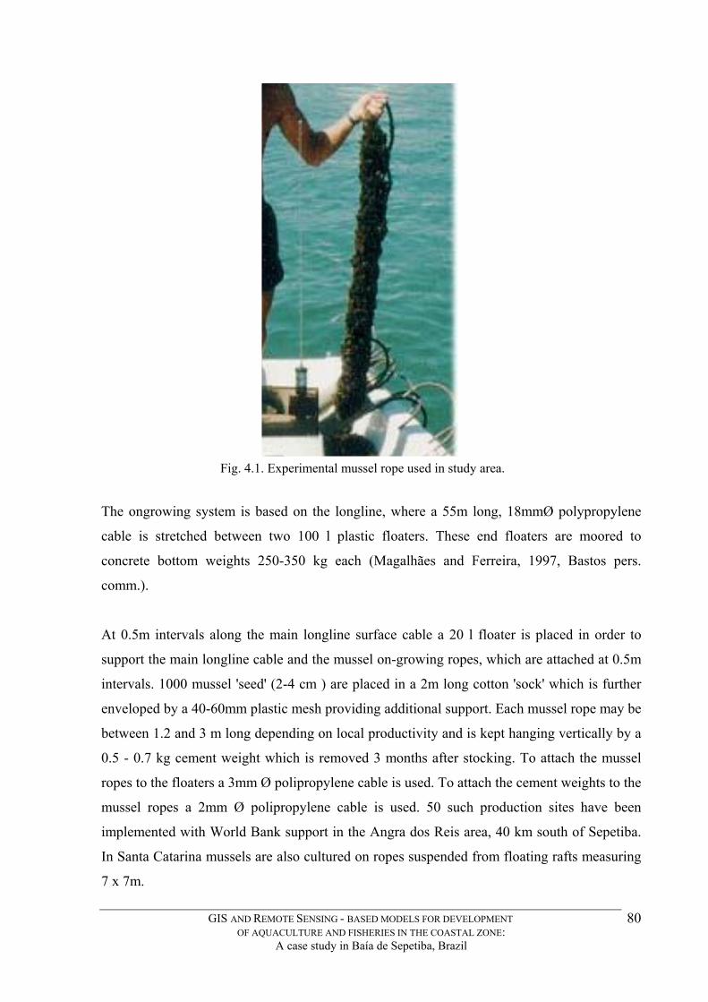
Fig. 4.1. Experimental mussel rope used in study area.

The ongrowing system is based on the longline, where a 55m long, 18mmØ polypropylene

cable is stretched between two 100 l plastic floaters. These end floaters are moored to

concrete bottom weights 250-350 kg each (Magalhães and Ferreira, 1997, Bastos pers.

comm.).

At 0.5m intervals along the main longline surface cable a 20 l floater is placed in order to

support the main longline cable and the mussel on-growing ropes, which are attached at 0.5m

intervals. 1000 mussel 'seed' (2-4 cm ) are placed in a 2m long cotton 'sock' which is further

enveloped by a 40-60mm plastic mesh providing additional support. Each mussel rope may be

between 1.2 and 3 m long depending on local productivity and is kept hanging vertically by a

0.5 - 0.7 kg cement weight which is removed 3 months after stocking. To attach the mussel

ropes to the floaters a 3mm Ø polipropylene cable is used. To attach the cement weights to the

mussel ropes a 2mm Ø polipropylene cable is used. 50 such production sites have been

implemented with World Bank support in the Angra dos Reis area, 40 km south of Sepetiba.

In Santa Catarina mussels are also cultured on ropes suspended from floating rafts measuring

7 x 7m.



80

This is system is used in low energy sites. Mussel production systems are generally set up

within close range (up to 200m ) of fishermen's homes, in sheltered shallow (5-25 m) coastal

waters.

In Santa Catarina (Anonymous, 1995) where mussel production is well established,

production is 2.5 kg of shucked meat per 1.2 m of rope. (Dressout of about 20%). Annual

production per 7 x 7 m module is 4 tons of shucked meat. Retail market price varies between

R$3,00 a R$5,00/kg (£0.62 - £1.03) (Scott et al, 2002). In Jurujuba, Niterói (Rio de Janeiro),

each mussel rope yields about 500 mussels (1kg - 6kg ) per year (with shells). This longline

cultivation system is the same analysed by Fagundes (1997) whose economic analysis

indicates a low operational cost and a profit returns at the lowest market price at the time of

the study (1996) R$1,00/kg (£0.21) even under the minimal husbandry practices. An estimate

of the potential economic value of mussel farming is given in table 4.1.

Table 4.1. Potential mussel production in Sepetiba.

Potential production t/ha/y-1 30 Dress-out % 20 Schucked meat t/ha 6 Mussel meat price (farm gate price) £/t 619.46

4.3.2 – Oysters 4.3.2.1 - Oysters production system.

The closest oyster farming region to Sepetiba is Cananéia, SP, south of Sepetiba. The system

adopted in Cananéia, São Paulo, consists of a metal rack measuring 10m x 1m supported on

cement legs and installed in the intertidal zone approximately 30cm above the seabed. 25

crossbars keep the stucture in shape. To this rack a 25mm netlon base measuring 1m x 10m

0.2m is fixed and used to support young ongrowing oysters. Once the oysters are in place, a

second mesh (8mm) is used for protection from predators as well as for shading. This system

is described by Fagundes et al (1996) and uses a final stocking density of 125-250 oysters m-2.

Market sized individuals (5 cm high) are obtained after 22 months. Figure 4.2 shows a similar

system of bamboo construction developed by artisanal fishermen in Itaucuruçá Island in

Sepetiba Bay.



81

Fig 4.2. Experimental oyster ongrowing racks in Sepetiba.

To obtain the oyster seed, or spats, two systems are commonly used. The first attracting the

oysters larvae present in mangrove waters onto aluminium strips, where they become fixed

and refered to as oyster spat. The strips are transferred to a solid polyprolilene support sheet

measuring 35 cm x 90 cm x 8 mm and are separated from each other by a 7 cm gap. Each

support sheet is holds 16 aluminium strips with oyster spat. These are placed on the

ongrowing racks. The supporting rack is covered with a 2.5 cm gauge ‘netlon’ netting.

The oyster support sheets are placed over the net on the racks, and enclosed with an 8 mm

gauge netting so as to protect the young oysters from predation. Using this method they attain

commercial size (5 cm.) in 22 months, with oyster densities ranging between 125 to 250 m-2 .

The second spat collection system uses scallop shells as substrate. Once collected, the scallop

shells are later re-arranged into 1m long strings where each substrate is separated from the

other by a 7 cm spacer, usually a pvc pipe section. Each string is composed of 14 layers.

Each rack may hold 100 strings. The lateral extremities are fixed so that currents will not

compress the strings overcrowding the oysters. The culture system is protected with the 8 mm

‘netlon’ netting. The Cananéia production system for C. rhizophorae is summarised in Table

4.2.



82

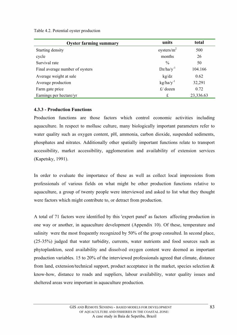
Table 4.2. Potential oyster production

Oyster farming summary units total Starting density oysters/m2 500 cycle months 26 Survival rate % 50 Final average number of oysters Dz/ha/y-1 104.166 Average weight at sale kg/dz 0.62 Average production kg/ha/y-1 32,291 Farm gate price £/ dozen 0.72 Earnings per hectare/yr £ 23,336.63

4.3.3 - Production Functions

Production functions are those factors which control economic activities including

aquaculture. In respect to mollusc culture, many biologically important parameters refer to

water quality such as oxygen content, pH, ammonia, carbon dioxide, suspended sediments,

phosphates and nitrates. Additionally other spatially important functions relate to transport

accessibility, market accessibility, agglomeration and availability of extension services

(Kapetsky, 1991).

In order to evaluate the importance of these as well as collect local impressions from

professionals of various fields on what might be other production functions relative to

aquaculture, a group of twenty people were interviewed and asked to list what they thought

were factors which might contribute to, or detract from production.

A total of 71 factors were identified by this 'expert panel' as factors affecting production in

one way or another, in aquaculture development (Appendix 10). Of these, temperature and

salinity were the most frequently recognized by 50% of the group consulted. In second place,

(25-35%) judged that water turbidity, currents, water nutrients and food sources such as

phytoplankton, seed availability and dissolved oxygen content were deemed as important

production variables. 15 to 20% of the interviewed professionals agreed that climate, distance

from land, extension/technical support, product acceptance in the market, species selection &

know-how, distance to roads and suppliers, labour availability, water quality issues and

sheltered areas were important in aquaculture production.



83

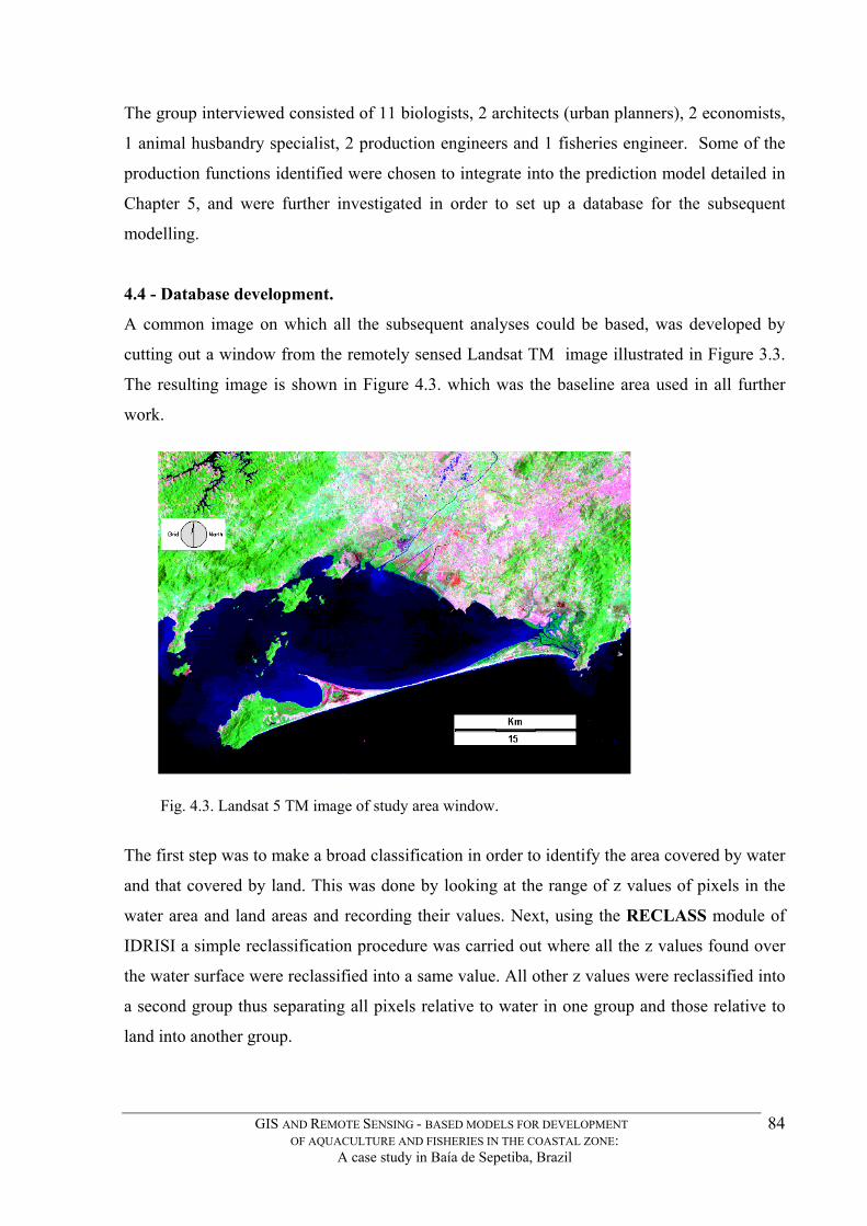
The group interviewed consisted of 11 biologists, 2 architects (urban planners), 2 economists,

1 animal husbandry specialist, 2 production engineers and 1 fisheries engineer. Some of the

production functions identified were chosen to integrate into the prediction model detailed in

Chapter 5, and were further investigated in order to set up a database for the subsequent

modelling.

4.4 - Database development.

A common image on which all the subsequent analyses could be based, was developed by

cutting out a window from the remotely sensed Landsat TM image illustrated in Figure 3.3.

The resulting image is shown in Figure 4.3. which was the baseline area used in all further

work.

Fig. 4.3. Landsat 5 TM image of study area window.

The first step was to make a broad classification in order to identify the area covered by water

and that covered by land. This was done by looking at the range of z values of pixels in the

water area and land areas and recording their values. Next, using the RECLASS module of

IDRISI a simple reclassification procedure was carried out where all the z values found over

the water surface were reclassified into a same value. All other z values were reclassified into

a second group thus separating all pixels relative to water in one group and those relative to

land into another group.



84

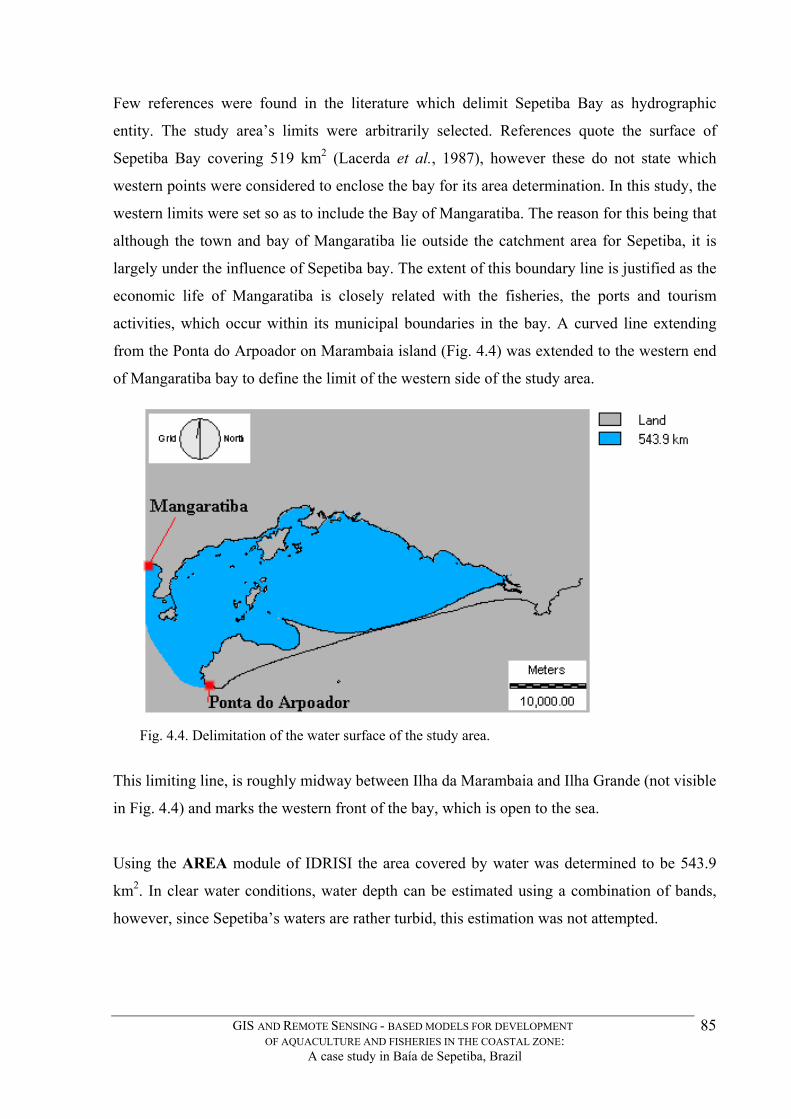
Few references were found in the literature which delimit Sepetiba Bay as hydrographic

entity. The study area’s limits were arbitrarily selected. References quote the surface of

Sepetiba Bay covering 519 km2 (Lacerda et al., 1987), however these do not state which

western points were considered to enclose the bay for its area determination. In this study, the

western limits were set so as to include the Bay of Mangaratiba. The reason for this being that

although the town and bay of Mangaratiba lie outside the catchment area for Sepetiba, it is

largely under the influence of Sepetiba bay. The extent of this boundary line is justified as the

economic life of Mangaratiba is closely related with the fisheries, the ports and tourism

activities, which occur within its municipal boundaries in the bay. A curved line extending

from the Ponta do Arpoador on Marambaia island (Fig. 4.4) was extended to the western end

of Mangaratiba bay to define the limit of the western side of the study area.

Fig. 4.4. Delimitation of the water surface of the study area.

This limiting line, is roughly midway between Ilha da Marambaia and Ilha Grande (not visible

in Fig. 4.4) and marks the western front of the bay, which is open to the sea.

Using the AREA module of IDRISI the area covered by water was determined to be 543.9

km2. In clear water conditions, water depth can be estimated using a combination of bands,

however, since Sepetiba’s waters are rather turbid, this estimation was not attempted.



85

4.4.1 - Scoring and Reclassifying

The thematic maps developed and incorporated into this study were scored in terms of their

suitability for the culture objectives. The scoring was achieved by using the reclassification

module RECLASS. The scoring system adopted in this study follows that used by Kapetsky

and Nath (1997). A 4-point scale was used, where the highest score (4) is adopted for the best

conditions (Most Suitable), for the purpose of the outcome, whereas the lowest score (1) is

reserved for areas which are inadequate (Unuitable). Areas may also be scored as (3) Suitable

or (2) Moderately Suitable. A four-point reclassification scheme with these categories of

suitability follows the methodology adopted by system is necessary.

4.5 - Environmental Factors

Aquaculture development depends on a series of physical and environmental variables. In

coastal waters some of the most important of these are: water temperature, salinity, and

dissolved oxygen because they limit aquatic species growth capacity. Other water quality

related parameters include the waters’ natural productivity and its dissolved inorganic

nutrients. To minimise risk of destruction to aquaculture installations, shelter from storms,

wind and waves also need to be considered.

Several environmental thematic layers necessary for modelling aquaculture in the study area

were created for the GIS, using techniques described in Chapter 3, one for each environmental

theme i.e. water temperature, salinity, dissolved oxygen content, chlorophilian biomass, faecal

coliform content, and natural indicators.

4.5.1 - Water temperature

Optimal water temperature for aquatic species is based on the sum of internal chemical

(mostly enzymatic) reactions. Different enzymes have different optimum temperatures

(Landau, 1992). The optimum temperature for an organism is that which allows the most

reactions to go on at efficiencies closest to the maximum (Landau, 1992).

In the case of the filter feeder Mytilus, selective filtration of algal cells goes on as long as

temperatures are 15º - 25ºC, but will slow down considerably when temperature either

increases or decreases (Landau, 1992).



86

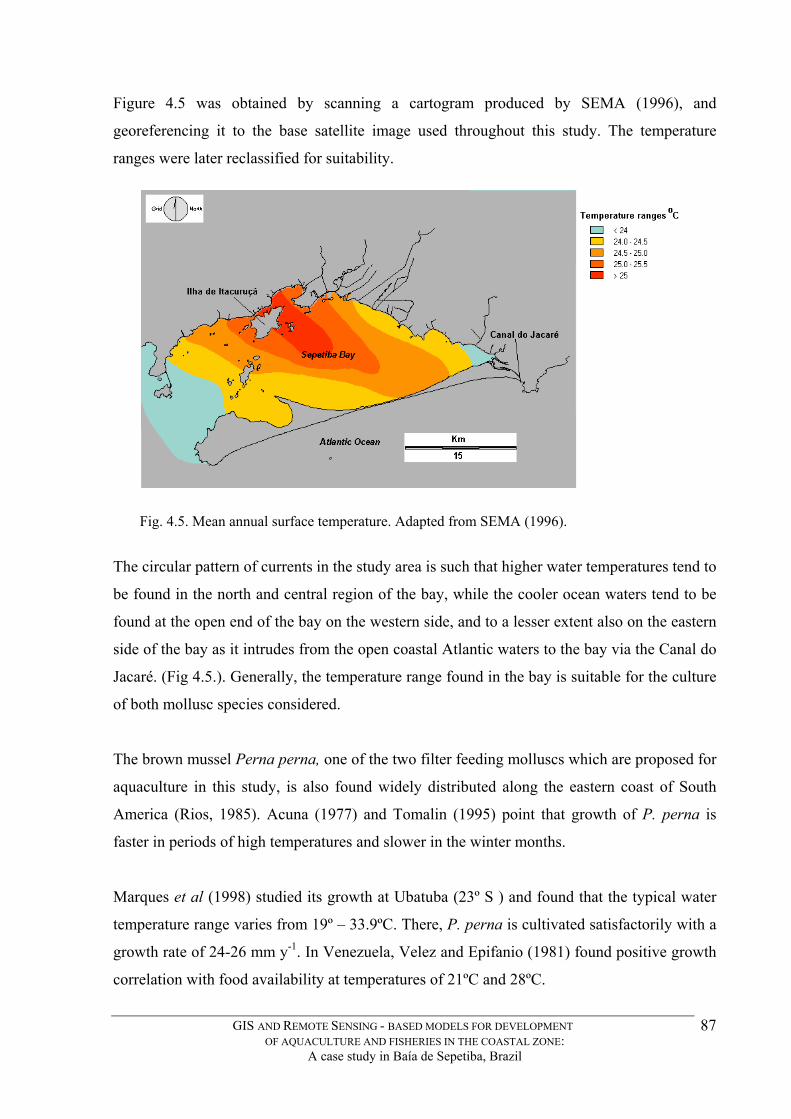
Figure 4.5 was obtained by scanning a cartogram produced by SEMA (1996), and

georeferencing it to the base satellite image used throughout this study. The temperature

ranges were later reclassified for suitability.

Fig. 4.5. Mean annual surface temperature. Adapted from SEMA (1996).

The circular pattern of currents in the study area is such that higher water temperatures tend to

be found in the north and central region of the bay, while the cooler ocean waters tend to be

found at the open end of the bay on the western side, and to a lesser extent also on the eastern

side of the bay as it intrudes from the open coastal Atlantic waters to the bay via the Canal do

Jacaré. (Fig 4.5.). Generally, the temperature range found in the bay is suitable for the culture

of both mollusc species considered.

The brown mussel Perna perna, one of the two filter feeding molluscs which are proposed for

aquaculture in this study, is also found widely distributed along the eastern coast of South

America (Rios, 1985). Acuna (1977) and Tomalin (1995) point that growth of P. perna is

faster in periods of high temperatures and slower in the winter months.

Marques et al (1998) studied its growth at Ubatuba (23º S ) and found that the typical water

temperature range varies from 19º – 33.9ºC. There, P. perna is cultivated satisfactorily with a

growth rate of 24-26 mm y-1. In Venezuela, Velez and Epifanio (1981) found positive growth

correlation with food availability at temperatures of 21ºC and 28ºC.



87

Schurink and Griffiths (1992) who investigated the physiological energetics of mussels in

South Africa found that P. perna grows faster at temperatures beyond 20ºC. Suplicy (pers.

com.) working in Southern Brazil with the same species, found from practical experience that

the best growing sites are found in areas which have a temperature range from 19º - 24ºC.

The second filter feeding mollusc considered in this study is C. rhizophorae. Water

temperature is also important for growth of C. rhizophorae or C. brasiliana, species which

are generally regarded as the same (Pereira et al., 1991). Their distribution range extends from

the Caribbean to Santa Catarina, Brazil. Pereira et al. (1988) successfully cultivated mangrove

oysters at Cananéia, São Paulo, in temperatures ranging from 18.2º – 31.4ºC. From Lemos et

al. (1994) who cultured mangrove oyster larvae and found maximum survival at 20ºC, it

seems that the younger stages require cooler waters. However, this study is limited to the

ongrowing phase of the activity. Due to the similarity of water temperature range for both

species considered, one scoring system was developed for both as shown in Table 4.3. Figure

4.6 shows the results of the reclassification.

Table 4.3. Water temperature suitability scoring for mollusc culture based on temperature (ºC)

Interpretation Score Most Suitable – good growth 25 - 28ºC 4 Suitable 20º - 25ºC 3 Moderately suitable 17º - 20ºC 2 Unsuitable < 17ºC >30ºC 1

Fig. 4.6. Temperature suitability reclassified image.



88

The reclassified image shows that that the region that contains the most suitable conditions is

that around Ilha de Itaucuruçá and the cental part of the bay, while all other areas falls within

the suitable category. This is a good indication as most of the areas found have coastlines

which potential for developing either longline mussel culture or rack-based oyster culture.

4.5.2 – Salinity

Mussels - Salinity is important in regulating the physiology of marine organisms although

changes in salinity do not affect the growth of bivalves as much as variation in temperature

(Laing and Spencer, 1997).

Figure 4.7 (SAL) shows the mean annual surface salinity in Sepetiba bay as found by FEEMA

(FEEMA, 1990). According to Marques et al. (1991) the mussel P. perna develops optimally

at salinities ranging from 31.5‰ to 35.8‰.

Fig. 4.7. Mean annual surface salinity (‰) concentration. Adapted from (FEEMA, 1996).

However, he successfully conducted culture of P. perna at stations where surface salinity

became as low as 12‰ in the rainy season (Marques et al., 1991). Although it is generally

agreed that P. perna is an organism preferring fully marine environments, there is no

published data on growth performance based on varying salinity conditions.



89

Suplicy (pers. com.) considers salinities between 30‰ to 40‰ to be feasible for P. perna

culture. SEBRAE (1996), reports the mussel culture experiments undertaken in Espirito

Santo, Brazil under salinity regimes ranging from 3.8‰ to 38‰.

SEBRAE (1996) notes that in sites where prolonged exposure to salinities lower than 10‰

occurred, significant mortality or reduction in growth did not follow. However, their yearly

average salinity for the two culture sites was 22.8‰ and 34.6‰. Most bivalves usually only

feed at higher salinities, so they should be sited where, for as long a period as possible,

salinity is within their optimum range (Laing and Spencer, 1997).

Table 4.4 shows the scoring system adopted in this study for the mussel growing area

selection. Figure 4.8 (SALTXT) shows the reclassified image based on the SEMA 1996. The

indication is that, with the exception of the areas close and around the fresh water sources

such as the rivers and canals in the northern side of the bay, most of the area is acceptable for

mussel culture.

Table 4.4. Suitability scoring for mussel growth based on salinity (‰).

Interpretation

Score

Most Suitable - Salinity fluctuation typical of most estuaries. > 22 ‰

4 Suitable - Lower or higher reaches of estuaries with more or less influence of fresh water of seawater. 18-22 ‰

3

Moderately Suitable - 14-18 ‰

2

Unsuitable - Areas where waters are prone to become dominated by salinities which are not optimal for growth <18 ‰

1



90

Although Figure 4.8 shows large areas in the central part of the bay reclassified as Most

Suitable for mussel culture, one must bear in mind that the salinity data available for this

study represents only the annual mean, which does not properly take into account large

surface salinity variations occuring during the rainy season, when vast amounts of freshwater

come into the bay forming surface ‘freshwater tongues’ extending far into the bay, as

evidenced in Fig 2.14 of Chapter 2, and as confirmed in field trip measurements.

Fig. 4.8. Surface salinity, reclassified suitability for mussel culture.

Although this is a seasonal condition, its duration may be enough to hinder mussel growth and

even cause production losses as their byssus holdfasts can weaken in conditions of extended

low salinities causing the mussels to drop from their culture installations. Thus, for a more

precise salinity suitability scoring, a more comprehensive survey would be needed on a larger

scale.

Oysters - Salinity requirements for oysters vary from species to species. Wakamatsu (1973)

considers C. brasiliana as a euryhaline species able to survive salinity ranging from 8‰ to

35‰, with the most suitable culture range between 15‰ to 25‰. Table 4.5 shows the scoring

system adopted in this study for the oyster growing area selection.



91

Table 4.5. Suitability scoring for oyster growth based on salinity (‰)

Interpretation Score Most suitable Salinity flutuation typical of most estuaries. 14-30‰

4

Suitable Lower or higher reaches of estuaries with more or less influence of fresh water of seawater. 28–30 ‰

3

Moderately suitable 32-34‰

2

Unsuitable Areas where waters are prone to become dominated by salinities which are not optimal for growth <8‰ > 34‰

1

Figure 4.9 shows that the bay can be roughly split into a western, more saline area and an

eastern, more brackish area, which is more suitable for oyster on-growing.

Fig. 4.9. Surface salinity, reclassified suitability for mangrove oyster culture.



92

This reclassification result is in agreement with the perception of the state fisheries

technicians and extension workers who have long elected the eastern end as the site for their

aquaculture lab site as mentioned in Chapter 2. The result of this reclassification is that a large

area in the central part of the bay is suitable for oyster culture (Fig 4.9). Most of the areas

classified as Most Suitable and Suitable fall in the

central and eastern half of the bay, much of it along

the northern coastline.

Figure 4.10 shows C. rhizophorae in its natural habitat

in Sepetiba Bay, among Rhizophora mangle prop

roots. These areas coincide with actual locations where

mangrove oysters grow, i.e. on remaining stands of

mangroves. To date, naturally produced oysters are

harvested mostly on the eastern end of the bay, which

is a good indication of the result of this

reclassification.

Fig. 4.10. C. rhizophorae oysters growing on mangrove prop roots.

4.5.3 - Dissolved oxygen content

Aquatic animals are generally very good at removing oxygen from the water. Dissolved

oxygen (DO) in aquatic culture is one of the most critical parameters for successful

aquaculture. In the marine environment, the action of waves, winds and currents usually

favours saturated levels of dissolved oxygen (8 –12 mg l-1). Under restricted culture volume

conditions, many aquaculturists will try to maintain a DO level of at least 5 mg l-1 (Landau,

1992).

Bivalve molluscs generally have a fairly high tolerance to low dissolved oxygen

concentrations and can also adapt by reducing their metabolic activity rate, to the extent of

using anaerobic respiration to provide energy needs (Laing and Spencer 1997).



93

A pumping oyster removes about 5 per cent of the oxygen content of the water passing

through the mantle cavity. Bivalve molluscs can close their valves in cases where water

conditions are poor, including when DO levels are low. Although they are able to withstand

long periods like this, they build up an ‘oxygen debt’ which has to be repaid when the are able

to restart pumping water through their systems (Walne, 1979).

Figure 4.11, shows the mean annual surface water dissolved oxygen concentration found in

Sepetiba bay (SEMA, 1996).

Fig. 4.11. Mean annual dissolved oxygen concentration mg l-1. Adapted from SEMA, 1996.

Table 4.6 shows the scoring system adopted in this study. It assumes that most aquatic species

need oxygen for their physiological needs, and also that they can withstand periods of low

concentrations.

A lower limit of 2 mg l-1 was set to take into account for events where these waters might

have an extra load of organic matter which will increase the Biological Oxygen Demand

(BOD) placing the culture organisms at risk for several hours or even maybe more than a day.



94

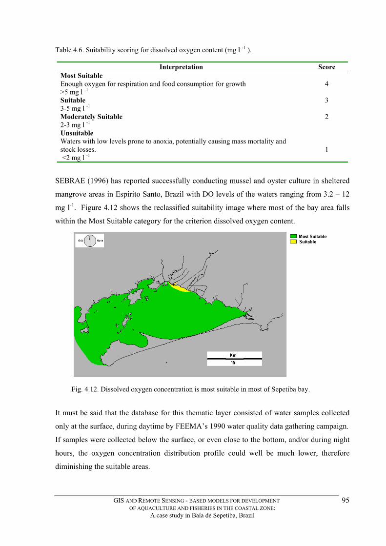
Table 4.6. Suitability scoring for dissolved oxygen content (mg l -1 ).

Interpretation Score Most Suitable Enough oxygen for respiration and food consumption for growth >5 mg l -1

4

Suitable 3-5 mg l -1

3

Moderately Suitable 2-3 mg l -1

2

Unsuitable Waters with low levels prone to anoxia, potentially causing mass mortality and stock losses. <2 mg l -1

1

SEBRAE (1996) has reported successfully conducting mussel and oyster culture in sheltered

mangrove areas in Espirito Santo, Brazil with DO levels of the waters ranging from 3.2 – 12

mg l-1. Figure 4.12 shows the reclassified suitability image where most of the bay area falls

within the Most Suitable category for the criterion dissolved oxygen content.

Fig. 4.12. Dissolved oxygen concentration is most suitable in most of Sepetiba bay. It must be said that the database for this thematic layer consisted of water samples collected

only at the surface, during daytime by FEEMA’s 1990 water quality data gathering campaign.

If samples were collected below the surface, or even close to the bottom, and/or during night

hours, the oxygen concentration distribution profile could well be much lower, therefore

diminishing the suitable areas.



95

Also, most of the sampling stations for the above data are well away from mangrove areas,

where higher levels of organic matter and detritus exist and could contribute towards lower

DO values. Lower subsurface DO levels would be detrimental especially to bottom culture of

oysters close to mangrove areas.

4.5.4 – Chlorophillian biomass

The amount of plant tissue built by photosynthesis over time is generally referred to as

primary production., so called because photosynthetic production is the basis of most marine

production. Bacteria are also capable of building up organic materials through chemosynthetic

mechanisms but these are of minor importance in the oceans as a whole (Lalli and

Thompsons, 1996). Phytoplankton biomass can be estimated by measuring chlorophyll-a

concentration. This is ideally measured by the 14C method should be measured as it is of more

ecological importance than instantaneous measures of standing stock or biomass. Primary

productivity is a difficult factor to assess for a given site as it is subject to seasonal abundance

and annual variation can fluctuate widely (Laing and Spencer, 1997).

Page and Hubbard (1987) studied Mytilus edulis growth in relation to water temperature and

potential food availability, and found that temporal variation in the growth of mussels

correlated with chlorophyll a concentration. Areas where mollusc rearing is the most intensive

such as Marennes–Oléron, France and Ria de Arosa, Spain have very high phytoplankton

biomasses (10-40 µgl-1) (Heral, 1991). Heral also notes that in coastal environments the

microphytobenthic biomass is from 2 to 25 times greater than the phytoplankton biomass, and

that strong tidal currents will replace this surface film in suspension, making it available for

filter feeding molluscs. Table 4.7 shows the suitability scoring criteria adopted for primary

productivity suitability scoring used in this study.



96

Table 4.7. Primary production suitability scoring for mussel growth based on Chlorophyll-a (µgl-1).

Interpretation Score Most Suitable Productive waters – Plentiful supply of phytoplankton for filter feeders. Good growth potential 18 – 30 (µgl-1)

4

Suitable Average growth conditions 10-18 (µgl-1)

3

Moderately suitable Areas with lower nutrients concentrations 6-10 (µgl-1)

2 Unsuitable Poor, oligotrophic waters, or areas with eutrophication propensity. < 6 >30 (µgl-1)

1

Coastal waters with river runoff tend to have a fertilising effect for phytoplankton, and this is

the case in Sepetiba, where there are 18 rivers and canals contributing nutrients for primary

production enhancement. Also, the study area has many shallow areas (0-3 m) where

microphytobenthos can develop. Chlorophyll a distribution information available for Sepetiba

bay is very scarce and limited and is shown in Fig. 4.13.

Fig. 4.13. Mean annual Chlorophyll a concentration distribution (µg l-1). Sampling stations

indicated. Adapted from (SEMA 1996). FEEMA sampling stations are indicated in red.



97

This chlorophyll a distribution represents the annual mean, which was based on eight

sampling stations monitored on a monthly basis for 10 months by FEEMA in the year 1990.

Since then, no further regular sampling surveys have been made covering large areas of the

bay. To make use of this dataset, the chlorophyll a choropleth map was scanned and

resampled in order to match the base satellite image used throughout this study.

In order to obtain a broader picture and complement the sparse chlorophyll a distribution

information available for the bay, especially in those areas furthest away from the sampling

stations used by FEEMA, an improvised chlorophyll a distribution map was created using the

available satellite imagery. This new map (Fig. 4.14) is an interpretation obtained by applying

the algorithm developed by Costa et al. (1998) for the coastal waters of the neighbouring state

of São Paulo, which has the same general characteristics as those which are found in Sepetiba

bay.

This model uses a relation between bands two and three of Landsat-5 TM. Costa et al. (1998)

found using the following equation:

Chlorophyll a concentration in µg l-1 = 0. 0.060914 + 0.109172 TM2 + 0.214841 TM3

Where TM2 = Band 2 of Landsat image, and TM3 = band 3 of Landsat image.

When this algorithm was applied to the satellite image containing the study area it produced a

range of values for Sepetiba Bay, comparable with that found by SEMA (1996). This range is

also similar to that found by Machado et al. (1998) where values between 3 to 20 µg l-1 Chl a

predominated in Sepetiba Bay.

To produce the improved primary production map layer used to indicate best areas for

mollusc farming, the module OVERLAY was used to overlay the satellite interpreted image

of Chl a (Fig. 4.14) together with the choropleth layer produced by SEMA (1996) (Fig. 4.13),

so that the highest values of each was retained in the resulting overlay. This resulting image

(Fig.4.15) was smoothed of abrupt differences between values, using a a 3 x 3 pixel FILTER.



98

Figure 4.15 shows a conspicuous high Chlorophyll-a concentration area in the central-eastern

portion of the bay which can be interpreted as a risk area in a mollusc farming scenario

because of the potential for noxious algal bloom eruptions.

Fig. 4.14. Chlorophyll-a (µgl-1) distribution interpreted from satellite image.

Fig. 4.15. Chlorophyll-a (µgl-1) distribution interpreted from satellite image and overlayed with SEMA (1996) survey data.



99

This eutrophication event could be triggered as the result of hypernutrification caused by raw

sewage discharging into the bay, and high temperature conditions. Such a plankton blooms

are rare in the area but may have to be considered carefully in local aquaculture development

projects.

The final reclassified image for mollusc farming areas (Fig 4.16) which was obtained by

applying the scoring criteria described in Table 4.7 shows 300.7 km2 of areas classified as

Most Suitable for mollusc farming.

Fig. 4.16. Site suitability as function of food availability indicated from reclassified Chlorophyll-a distribution.

These areas are present in the northeasten part of the bay where mangrove oysters naturally

grow, as well as in the southwestern areas where brown mussels grow. They also include all

the areas in and around mangroves where high natural productivity occurs.

As far as Chl a concentration is concerned, few areas were classified as Unsuitable. Two such

areas occur, one of which lies in front of a major freshwater discharge which is the Canal de

São Francisco and is probably more an indication of high sediment loading in the water

instead of actual high Chl a content. The second such area is visible as a long narrow strip

extending from the Rio Piracão on the southern edge of the bay westwards along the Restinga

da Marambaia probably due to re-suspension of fine particles of bottom sediments carried by

longshore currents, or alternatively genuinely high Chl-a values as a result of microbenthic

algal activity in very shallow water.



100

4.5.5 - Faecal coliforms

Bivalves selectively filter phytoplankton from the seawater during feeding. However, in the

process they take in some bacteria and viruses.

Some of these, especially those originating from domestic sewage discharges, which typically

contain pathogenic bacteria such as Salmonella sp., Shighella sp., Clostrdium and

nonpathogenic Escherichia coli can cause serious illness in human consumers if they remain

in the bivalve when it is eaten (Laing and Spencer 1997, Shumway 1992). In the UK it is a

statutory requirement that shellfish beds from which harvested bivalves are intended for

consumption must be classified according to the faecal coliform levels of the bivalve flesh

(Table 4.8).This classification is issued initially on a provisional basis after sampling

fortnightly for 3-4 months and a full classification may be achieved after a year of continuous

sampling at monthly intervals. The EC has established directive 91/492/CEE in 15.07.91

published in DOCE number L268 which states the conditions for production areas including

the location and the boundaries of production areas are to be fixed by the competent authority,

and are classified into three groups.

Case 1 areas:

1. The possession of visual characteristics associated with freshness and viability, including

shells free of dirt, an adequate response to percussion, and normal amounts of intravalvular

liquid.

2. They must contain less than 300 faecal coliforms or less than 230 E. Coli per 100 g of

mollusc flesh and intravalvular liquid based on a five-tube, three-dilution MPN-test or any

other bacteriological procedure shown to be of equivalent accuracy.

3. They must not contain salmonella in 25 g of mollusc flesh. (http://158.169.50.70/eur-

lex/en/lif/dat/1991/en_391L0492.html).

Case 2 areas: molluscs can be collected but only placed on the market for human consumption

after treatment in a purification centre, after relaying. Live bivalve molluscs from these areas

must not exceed the limits of a five-tube, three-dilution MPN-test of 6,000 faecal coliforms

per 100 g of flesh or 4,600 E. Coli per 100 g of flesh in 90 % of samples.

molluscs can be collected for direct human consumption and must comply with

the following requirements:



101

Case 3 areas: , molluscs can be collected but only placed on the market after relaying (moving

the molluscs to approved areas) over a long period (at least two months), whether or not

combined with purification, or after intensive purification for a period. Live bivalve molluscs

from these areas must not exceed the limits of a five-tube, three-dilution MPN-test of 60,000

faecal coliforms per 100 g of flesh.

Table 4.8. Criteria for classifying shellfish harvesting areas in the UK. Source Laing and Spencer (1997).

Classification

category Faecal coliform bacteria (E. coli per 100 g flesh)

Comment

A

Less tha 300 (<230 E.c.) in all samples

Suitable for consumption

B

Less than 6,000 Depuration needed (or relaying in a category A area or cooking by an approved method)

C

less than 60,000 in all samples

Prohibited Above 60,000 Cannot be taken for placing on the market.

Relaying (minimum of 2 months) in category A or B area needed (or cooking by an approved method)

In the absence of habitual methods of detection of virus and virological norms, sanitary

control will be based on faecal bacteria (Casabellas, 1991).

In Brazil, the national environment council (CONAMA) specifies the following water quality

faecal coliform tolerances for marine and brackish marine waters (Classes 5 and 7)

specifically for the purpose of harvesting or farming aquatic species:

“No more than 14 faecal coliforms per 100 ml for animals which will be

consumed uncooked. No more than 10% of the samples exceeding 43 faecal

coliforms per 100 ml.

For other uses a limit no greater than 1,000 coliforms per 100 ml or more in

at least 5 samples collected monthly, on any month”. (CONAMA, 1986).

The Brazilian Food Health Standards Committee (DINAL) classifies molluscan shellfish

according to the waters from which they are harvested and Table 4.9 shows the

reclassification scheme developed for this study based on the TCN which refers to total

coliform number per ml.



102

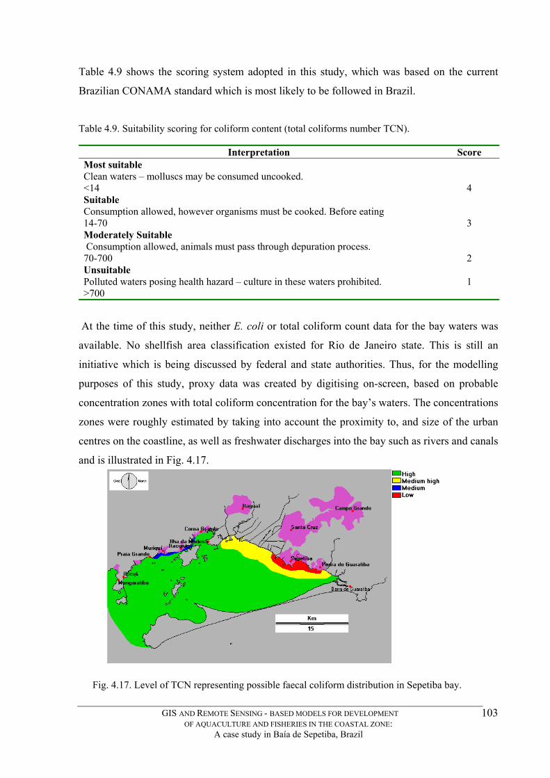
Table 4.9 shows the scoring system adopted in this study, which was based on the current

Brazilian CONAMA standard which is most likely to be followed in Brazil.

Table 4.9. Suitability scoring for coliform content (total coliforms number TCN).

Interpretation Score Most suitable Clean waters – molluscs may be consumed uncooked. <14

4 Suitable Consumption allowed, however organisms must be cooked. Before eating 14-70

3 Moderately Suitable Consumption allowed, animals must pass through depuration process. 70-700

2 Unsuitable Polluted waters posing health hazard – culture in these waters prohibited. >700

1

At the time of this study, neither E. coli or total coliform count data for the bay waters was

available. No shellfish area classification existed for Rio de Janeiro state. This is still an

initiative which is being discussed by federal and state authorities. Thus, for the modelling

purposes of this study, proxy data was created by digitising on-screen, based on probable

concentration zones with total coliform concentration for the bay’s waters. The concentrations

zones were roughly estimated by taking into account the proximity to, and size of the urban

centres on the coastline, as well as freshwater discharges into the bay such as rivers and canals

and is illustrated in Fig. 4.17.

Fig. 4.17. Level of TCN representing possible faecal coliform distribution in Sepetiba bay.



103

The zone of highest potential organic and bacterial pollution from sewage discharges is

known to be close to the town of Sepetiba where an underwater pipeline discharges raw

sewage into the bay. Algal blooms sporadically (about once very 7 years) occur in northern

coastline of the bay in front of Sepetiba forming a long, narrow ‘tongues’ extending in an

East-West direction folloeing long-shore currents. Hypernutrification of these waters is

associated with accompanying high bacterial counts.

Figure 4.18 shows the reclassified suitability map image, which when analysed with the

AREA module indicates 478 km2 of Most Suitable areas and another 48 km2 of Suitable areas

with only 4 km2 of Moderately Suitable areas and 14 km2 of unsuitable areas. This proxy

evaluation shows that about 88% of the bay falls within the Most Suitable category, a

promising indication for the development of the activity.

Fig. 4.18. Suitable areas for bivalve culture in Sepetiba bay.

4.5.6 - Natural Indicators

A good natural indicator of appropriate water conditions for C. rhizophora oyster growth, is

the set of existing conditions where it already thrives. These are found in the local mangroves.

In this way, a supervised classification procedure was carried out identifying all mangrove

areas in Sepetiba bay using a 354 RGB colour composite. To these areas a buffer zone of 100

meters was added in the belief that similar conditions prevailed within this range.



104

Similarly, natural conditions for development of P. perna exist mainly on the rocky littoral

zone of islands in the bay.

4.6 - Infrastructure:

Aquaculture development depends on a series of infrastructural elements, some relating to

physical infrastructure others relating to social aspects . Some of these include:

4.6.1 -Technical support

Several stages of aquaculture development demand the support of specialized technicians.

These are usually fisheries and aquaculture extension personnel paid by local governments.

They are important in passing scientific know-how which enables the activity in its different

stages. The know-how or technical support layer, was developed by considering the location

of the main fisheries extension office in Rio de Janeiro, 60 km from the bay, as sufficient in

terms of number of people and close enough to cover the advice needs for at least the initial

phases of aquaculture development and production. In this way, a ‘technical support’ layer

was created with a Most Suitable classification encompassing the whole study area.

4.6.2 -Road Network -

Transportation

The extent of the road network and its quality are important for the flow of raw materials and

services to and from the production sites, as well as allows production to reach local, regional

and foreign markets. Solutions to aquaculture problems sometimes depend on the prompt

arrival of a technician or piece of equipment to the production site. Transportation by boat

may also be effective. The suitability scoring criteria are shown in Table 4.10. Due to the

topography of the region, the road network in the western part of the continent in the study

area is slightly more distant from the shoreline because it is in flat coastal lands. Access to the

water, by road, is limited to mainly three towns (Fig. 4.19). In contrast, the coastal mountains

which predominate in the eastern side make for a short distances between shoreline and

service roads.



105

Table 4.10. Suitability scoring for accessibility to road network.

Interpretation Score Most suitable Close access to roads on the continent coastline, or short distance from it 0-5 km

4

Suitable Medium accessibility, away from road network 5-9 km

3

Moderately Suitable 9-14

2

Unsuitable >14 km

1

Fig. 4.19. Mollusc suitability reclassified from roads network.

4.6.3 – Fishing Communities

4.6.3.1 – Location of Fishermen

Local Fishermen, are naturally the human resources most indicated in developing coastal

aquaculture.As with other livestock, close range to holding facilities/cultivation systems

favours less cost in maintenance and facilitates surveillance. Their presence in and around the

bay was introduced into the GIS as a series of locations where fishermen have established

addresses such as a coop house, or representation, as well as knowledge collected in field

trips.



106

Table 4.11 shows the scoring system utilised for reclassifying the study area in terms of the

distance between fishermen locations and potential culture sites. The results of this

reclassification are illustrated in Figure 4.20.

Fig. 4.20. Suitability of mollusc cultivation sites as a function of distance from fishermen homes or coop sites.

Table 4.11. Suitability scoring adopted for distance of potential cultivation sites (km) from fishermen

residences or co-ops.

Interpretation Score Within visual distance or close surveillance <0.9

4

Acceptable range, with added transportation costs 0.9 < 1.5

3

Only in possible with locally resident support 1.5 – 3.0

2

> 3 1

4.6.4 - Seed sources

4.6.4.1 - Mussel seed

Mussel seed sources are essential to the development of the ongrowing phase. Mussel seed

can be scraped off rocks where they grow, or alternately their spat can be gathered at the

appropriate times of the year from artificial collectors placed in sites close to where they grow

and breed. The scoring system adopted in Table 4.12 was based on the travel distance from

the main concentrations of fishermen houses or co-ops to the mussel seed sources.



107

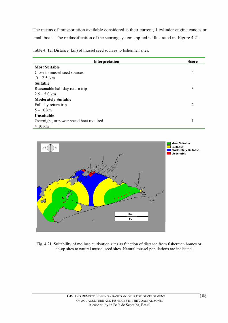
The means of transportation available considered is their current, 1 cylinder engine canoes or

small boats. The reclassification of the scoring system applied is illustrated in Figure 4.21.

Table 4. 12. Distance (km) of mussel seed sources to fishermen sites.

Interpretation Score Most Suitable Close to mussel seed sources 0 – 2.5 km

4

Suitable Reasonable half day return trip 2.5 – 5.0 km

3

Moderately Suitable Full day return trip 5 – 10 km

2

Unsuitable Overnight, or power speed boat required. > 10 km

1

Fig. 4.21. Suitability of mollusc cultivation sites as function of distance from fishermen homes or co-op sites to natural mussel seed sites. Natural mussel populations are indicated.



108

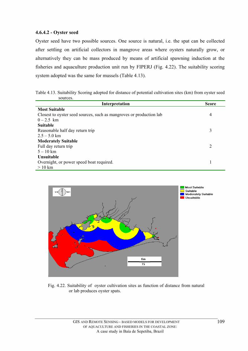
4.6.4.2 - Oyster seed

Oyster seed have two possible sources. One source is natural, i.e. the spat can be collected

after settling on artificial collectors in mangrove areas where oysters naturally grow, or

alternatively they can be mass produced by means of artificial spawning induction at the

fisheries and aquaculture production unit run by FIPERJ (Fig. 4.22). The suitability scoring

system adopted was the same for mussels (Table 4.13).

Table 4.13. Suitability Scoring adopted for distance of potential cultivation sites (km) from oyster seed sources.

Interpretation Score Most Suitable Closest to oyster seed sources, such as mangroves or production lab 0 – 2.5 km

4

Suitable Reasonable half day return trip 2.5 – 5.0 km

3

Moderately Suitable Full day return trip 5 – 10 km

2

Unsuitable Overnight, or power speed boat required. > 10 km

1

Fig. 4.22. Suitability of oyster cultivation sites as function of distance from natural

or lab produces oyster spats.



109

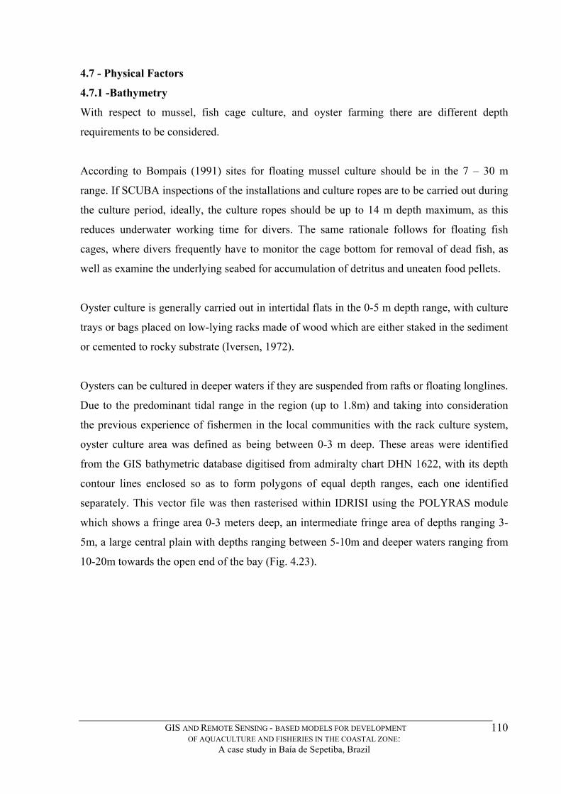
4.7 - Physical Factors

4.7.1 -Bathymetry

With respect to mussel, fish cage culture, and oyster farming there are different depth

requirements to be considered.

According to Bompais (1991) sites for floating mussel culture should be in the 7 – 30 m

range. If SCUBA inspections of the installations and culture ropes are to be carried out during

the culture period, ideally, the culture ropes should be up to 14 m depth maximum, as this

reduces underwater working time for divers. The same rationale follows for floating fish

cages, where divers frequently have to monitor the cage bottom for removal of dead fish, as

well as examine the underlying seabed for accumulation of detritus and uneaten food pellets.

Oyster culture is generally carried out in intertidal flats in the 0-5 m depth range, with culture

trays or bags placed on low-lying racks made of wood which are either staked in the sediment

or cemented to rocky substrate (Iversen, 1972).

Oysters can be cultured in deeper waters if they are suspended from rafts or floating longlines.

Due to the predominant tidal range in the region (up to 1.8m) and taking into consideration

the previous experience of fishermen in the local communities with the rack culture system,

oyster culture area was defined as being between 0-3 m deep. These areas were identified

from the GIS bathymetric database digitised from admiralty chart DHN 1622, with its depth

contour lines enclosed so as to form polygons of equal depth ranges, each one identified

separately. This vector file was then rasterised within IDRISI using the POLYRAS module

which shows a fringe area 0-3 meters deep, an intermediate fringe area of depths ranging 3-

5m, a large central plain with depths ranging between 5-10m and deeper waters ranging from

10-20m towards the open end of the bay (Fig. 4.23).



110

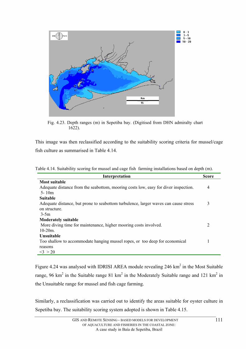
Fig. 4.23. Depth ranges (m) in Sepetiba bay. (Digitised from DHN admiralty chart 1622).

This image was then reclassified according to the suitability scoring criteria for mussel/cage

fish culture as summarised in Table 4.14.

Table 4.14. Suitability scoring for mussel and cage fish farming installations based on depth (m).

Interpretation Score Most suitable Adequate distance from the seabottom, mooring costs low, easy for diver inspection. 5- 10m

4

Suitable Adequate distance, but prone to seabottom turbulence, larger waves can cause stress on structure. 3-5m

3

Moderately suitable More diving time for maintenance, higher mooring costs involved. 10-20m.

2

Unsuitable Too shallow to accommodate hanging mussel ropes, or too deep for economical reasons <3 > 20

1

Figure 4.24 was analysed with IDRISI AREA module revealing 246 km2 in the Most Suitable

range, 96 km2 in the Suitable range 81 km2 in the Moderately Suitable range and 121 km2 in

the Unsuitable range for mussel and fish cage farming.

Similarly, a reclassification was carried out to identify the areas suitable for oyster culture in

Sepetiba bay. The suitability scoring system adopted is shown in Table 4.15.



111

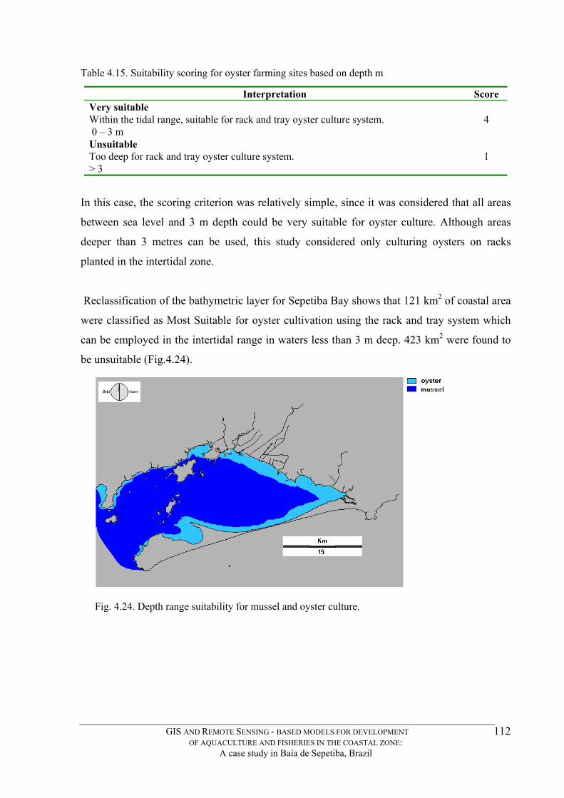
Table 4.15. Suitability scoring for oyster farming sites based on depth m

Interpretation Score Very suitable Within the tidal range, suitable for rack and tray oyster culture system. 0 – 3 m

4

Unsuitable Too deep for rack and tray oyster culture system. > 3

1

In this case, the scoring criterion was relatively simple, since it was considered that all areas

between sea level and 3 m depth could be very suitable for oyster culture. Although areas

deeper than 3 metres can be used, this study considered only culturing oysters on racks

planted in the intertidal zone.

Reclassification of the bathymetric layer for Sepetiba Bay shows that 121 km2 of coastal area

were classified as Most Suitable for oyster cultivation using the rack and tray system which

can be employed in the intertidal range in waters less than 3 m deep. 423 km2 were found to

be unsuitable (Fig.4.24).

Fig. 4.24. Depth range suitability for mussel and oyster culture.



112

4.7.2 – Shelter

4.7.2.1 -Exposure

Protected or sheltered areas are important in aquaculture development as they require less

investment in mooring structures and are less prone to damage. A layer consisting of shelter

from exposure to severe weather conditions was created.

Since waves are a good indicator of exposed conditions, wave height was chosen as a layer to

be developed which would give a good indication of sheltered areas. According to Beveridge

(1996) most inshore floating cage structures are designed to withstand significant wave

heights only up to about 1 - 1.5 m. Floating mussel longlines are more flexible than floating

cage structures and can withstand more severe weather conditions than most rigid-structured

floating cages.

Exposure conditions for floating mussel longlines and fish cages were considered to be of

equal resistance to wave conditions. 4.7.2.2 -Calculating wave heights

Wave height can be predicted using water depth, wind speed and wind fetch data for a

particular point in space. To create a thematic map layer with potential wave heights for the

study area, an IDRISI macro was constructed incorporating the formula proposed in the U.S.

Army Corps of Engineers Shore Protection Manual, 1984, for forecasting waves in shallow

waters.

H speed depth

Speed

Fetch Speed

depth

Speed

=

0 283 0 530 9 8

0 00565 9 8

0 530 9 8

9.8

0 75

0.5

0 75 . tanh . .

tanh

. .

tanh . .

.

.

.

Where: speed = wind surface speed, fetch = distance over unimpeded water surface, depth = depth in m.



113

In order to carry out the calculation of the maximum significant wave height in shallow

waters within the facility of IDRISI's image calculator, it was broken down into 7 steps as

shown in Table 4.16.

Table 4.16. Idrisi image calculator expressions to determine maximum significant wave heights for the Sepetiba bay area. (Enclosed in brackets are names of images used. Result of each expression is another image)

Expression

A 530*(((9.8*[DEPTH])/[SPEED2])^.75) = wave1 B .00565*((9.8*[ DEPTH])/[SPEED2]/[SPEED2])^.5) = wave2 C ((2.718^[WAVE1])-(2.718^-[WAVE1]))/((2.718^[WAVE1])+(2.718^-[WAVE1]))

= wave3 D [WAVE2]/[WAVE3] = wave4 E ((2.718^[WAVE4])-(2.718^-[WAVE4]))/((2.718^[WAVE4])+(2.718^-[WAVE4]))

= wave5 F (0.283*[WAVE3])*[WAVE5] = wave6. G ([SPEED2]*[WAVE6])/9.8 = wave7

However, it was finally decided that by using a multi-step macro which broke each equation

down to its simplest form was better. In this way, alternative wind velocities and wind

fetches, can be investigated in subsequent studies. This detailed macro is found in Appendix 8

and enables the calculation of wave height for any pixel across the water surface using the

layers containing depth value, wind fetch and wind speed.

4.7.2.3 - Depth layer

The depth information necessary for the significant wave height calculation was made

available as a bathymetric thematic layer which was digitised from Admiralty chart 1622 (Fig.

4.23). The creation of this layer (BATHYDIS) is described earlier in section 4.7.1. The depth

ranges used for determining maximum significant wave height used in this study were 0-3m,

3-5m, 5-10m and 10-20m. 4.7.2.4 -Creating the wind speed and wind fetch layers

Wind Speed

Wind speed was assigned as an attributed value directly to the pixels covering all the water

surface area. Two wind directions were used: that due North-east and that due South-east.



114

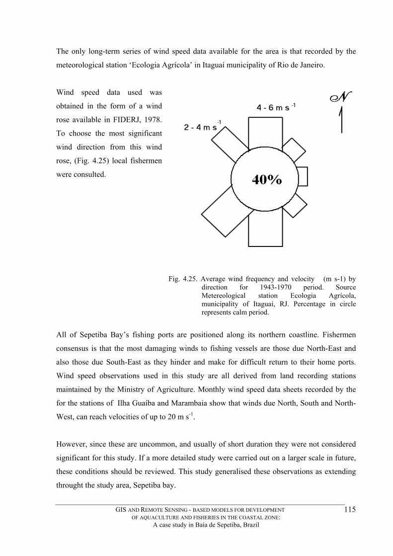
The only long-term series of wind speed data available for the area is that recorded by the

meteorological station ‘Ecologia Agrícola’ in Itaguaí municipality of Rio de Janeiro.

Wind speed data used was

obtained in the form of a wind

rose available in FIDERJ, 1978.

To choose the most significant

wind direction from this wind

rose, (Fig. 4.25) local fishermen

were consulted.

Fig. 4.25. Average wind frequency and velocity (m s-1) by

direction for 1943-1970 period. Source Metereological station Ecologia Agrícola, municipality of Itaguaí, RJ. Percentage in circle represents calm period.

All of Sepetiba Bay’s fishing ports are positioned along its northern coastline. Fishermen

consensus is that the most damaging winds to fishing vessels are those due North-East and

also those due South-East as they hinder and make for difficult return to their home ports.

Wind speed observations used in this study are all derived from land recording stations

maintained by the Ministry of Agriculture. Monthly wind speed data sheets recorded by the

for the stations of Ilha Guaíba and Marambaia show that winds due North, South and North-

West, can reach velocities of up to 20 m s-1.

However, since these are uncommon, and usually of short duration they were not considered

significant for this study. If a more detailed study were carried out on a larger scale in future,

these conditions should be reviewed. This study generalised these observations as extending

throught the study area, Sepetiba bay.



115

In this way an image (Fig. 4.26) was created with a wind velocity speed of 4 ms-1, generalised

over the whole area of the bay’s water surface.

Fig. 4.26. Wind speed layer for study area.

Wind Fetch

Fetch is the stretch of water over which the wind blows (Sverdrup et al., 1970). The greater

the fetch, the greater potential for generating higher waves (US Army Corps of Engineers,

1984). As can be seen in Figure 4.26, In Sepetiba Bay, fetch is mostly limited to the stretch of

open water which lies between the sand barrier beach (Marambaia Island) and the continent,

which is approximately 16 km at its widest. However, there is one relatively narrow area in

the bay, which potentially has an almost unimpeded fetch from the open Atlantic Ocean. This

is located between Ilha Grande and Ilha da Marambaia.

In this study, wind fetches were considered as starting from the edges of feature edges in the

study area. Since the bay is mostly enclosed, the starting point for the Northeast wind fetch

begins at the land/water interface of all SW lying features such as the islands and the Ilha da

Marambaia sand barrier beach. Where the bay was open to the Atlantic ocean, the fetch

begins at a short distance away from the coastline in the open Atlantic.

Due to the geographic disposition of the bay, winds due East or West will normally have the

long fetches, however these are very rare in the region, as can be seen in the wind rose (Fig.

4.25).



116

Because the bay is protected by Ilha da Marambaia, a 40 km sand barrier beach on it’s

southern boundary, winds due North-east have limited action. However, there is one

significant gap between Ilha Grande to the west and Ilha da Marambaia, which allows for

longer fetches which in reality are the most damaging. Winds due South-east are considered

the second most damaging.

To create the wind fetch layer the methodology presented by UNITAR (1995) was employed.

The module INITIAL of IDRISI, was used to create two ‘force images’ for the study area

using the a magnitude direction of 45º to represent a force equivalent to the direction wind

due NE, and another image with a magnitude direction of 135º to represent wind due SE.

These two images are proposed as the wind fetch layers, used in an image algebra calculation

in order to obtain a layer with the maximum significant wave height distribution over the bay.

To determine the fetch length along these two directions, a dispersion routine (DISPERSE

module) was used, with zero as a starting value on the feature edges such as the coastline, or

at the water boundary (Atlantic Ocean). The DISPERSE routine, attributes incremental

values to pixels along the wind fetch path. To obtain the distance at any point along the fetch

surface, the pixel values were multiplied by the pixel resolution, which for this Landsat

satellite image is 30m. These operations are summarised in Figure 4.27.



117

Fig. 4.27. Summary of wind fetch image creation.

Values outside the water surface were discarded by an OVERLAY (multiply) operation

where a template image in which all pixels not over water surface were attributed a value of

zero. Figures 4.28 and 4.29 show the resulting images fetch layers for winds due NE ans SE

reclassified into three broad significant fetch range categories: 0-5 km, 5-10 km and 10-15 km

fetches.



118

Fig. 4.28. Wind fetch layer for wind due NE, reclassified for study area.

Fig. 4.29. Wind fetch layer for wind due SE, reclassified for study area. 4.7.2.5 - Maximum Significant Wave Height

Creating the layer Maximum Significant Wave Height layer entailed using the wind fetch,

wind speed and water depth thematic layers in the macro developed in the beginning of this

chapter, which incorporates the significant wave height prediction formula. Thus two wave

height layers were created: one for waves generated by winds due NE, and another for waves

generated from winds due SE. Figure 4.30 shows the predicted distribution of wave heights

for Sepetiba Bay, based on depths, wind speed and fetch for wind due NE.



119

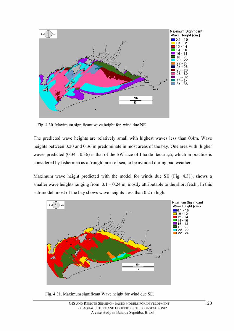
Fig. 4.30. Maximum significant wave height for wind due NE.

The predicted wave heights are relatively small with highest waves less than 0.4m. Wave

heights between 0.20 and 0.36 m predominate in most areas of the bay. One area with higher

waves predicted (0.34 - 0.36) is that of the SW face of Ilha de Itacuruçá, which in practice is

considered by fishermen as a ‘rough’ area of sea, to be avoided during bad weather.

Maximum wave height predicted with the model for winds due SE (Fig. 4.31), shows a

smaller wave heights ranging from 0.1 – 0.24 m, mostly attributable to the short fetch . In this

sub-model most of the bay shows wave heights less than 0.2 m high.

Fig. 4.31. Maximum significant Wave height for wind due SE.



120

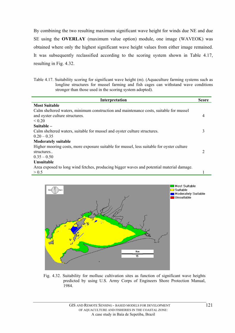
By combining the two resulting maximum significant wave height for winds due NE and due

SE using the OVERLAY (maximum value option) module, one image (WAVEOK) was

obtained where only the highest significant wave height values from either image remained.

It was subsequently reclassified according to the scoring system shown in Table 4.17,

resulting in Fig. 4.32.

Table 4.17. Suitability scoring for significant wave height (m). (Aquaculture farming systems such as longline structures for mussel farming and fish cages can withstand wave conditions stronger than those used in the scoring system adopted).

Interpretation Score

Most Suitable Calm sheltered waters, minimum construction and maintenance costs, suitable for mussel and oyster culture structures. < 0.20

4

Suitable – Calm sheltered waters, suitable for mussel and oyster culture structures. 0.20 – 0.35

3

Moderately suitable Higher mooring costs, more exposure suitable for mussel, less suitable for oyster culture structures.. 0.35 – 0.50

2

Unsuitable Area exposed to long wind fetches, producing bigger waves and potential material damage. > 0.5

1

Fig. 4.32. Suitability for mollusc cultivation sites as function of significant wave heights predicted by using U.S. Army Corps of Engineers Shore Protection Manual, 1984.



121

4.7.3 - Surface currents

Consideration of water hydrodynamics is important for water based aquaculture. Under

favourable conditions bivalves will remain open and pumping water for most of the day. The

major role of the water current is undoubtedly feeding, but it also carries away waste products

and brings in a supply of oxygen (Walne, 1979).

As current velocities increase, construction costs for cages and installing moorings increase

(Beveridge , 1996). Aquaculture production can increase with increased current velocity as it

brings new supplies of oxygen, phytoplankton and food particles important for mollusc

culture, as well as provides for removing faeces, and wastes. Stocking rates can also increase.

Beyond a certain point, current action can be detrimental to the installations by deforming fish

net enclosures resulting in less volume for fish, causing crowding and increasing stress. With

increased current velocities fish also have to expend more energy maintaining their position in

space, adversely affecting their growth.

For bivalve cultivation Laing and Spencer, (1997) consider that sheltered areas with tidal

flows of 0.5 –1.0 m s-1 provide the best conditions, giving sufficient water exchange to supply

the animals with an adequate supply of food and oxygen and for the removal of wastes. They

also consider that for tray cultivation of oysters, sites that have only a minimal flow of water

where water is exchanged by the tides can be successful. Hickman (1992), found current

flows recorded at several longline and raft mussels cultivation sites to vary from 0.03 – 1.5 m

s-1. The suitability scoring adopted for this study is summarised in Table 4.18. Knowledge of

current patterns and velocities for Sepetiba Bay is still very limited.

Table 4.18. Suitability scoring for current speed (m s-1).

Interpretation Score Most suitable Enables good flow food supply, while carrying away wastes. 0.5 – 1.0

4

Suitable 0.3- 0.5 and 1.0 –1.3

3

Moderately suitable Areas which could have trouble in case of toxic algal blooms 0.1 – 0.3 and 1.3 – 1.5

2

Unsuitable Slow flows can lead to build up of toxins, organic matter and anoxia Swifter currents may cause stress on organisms as well as culture structures. < 0.1 > 1.5

1



122

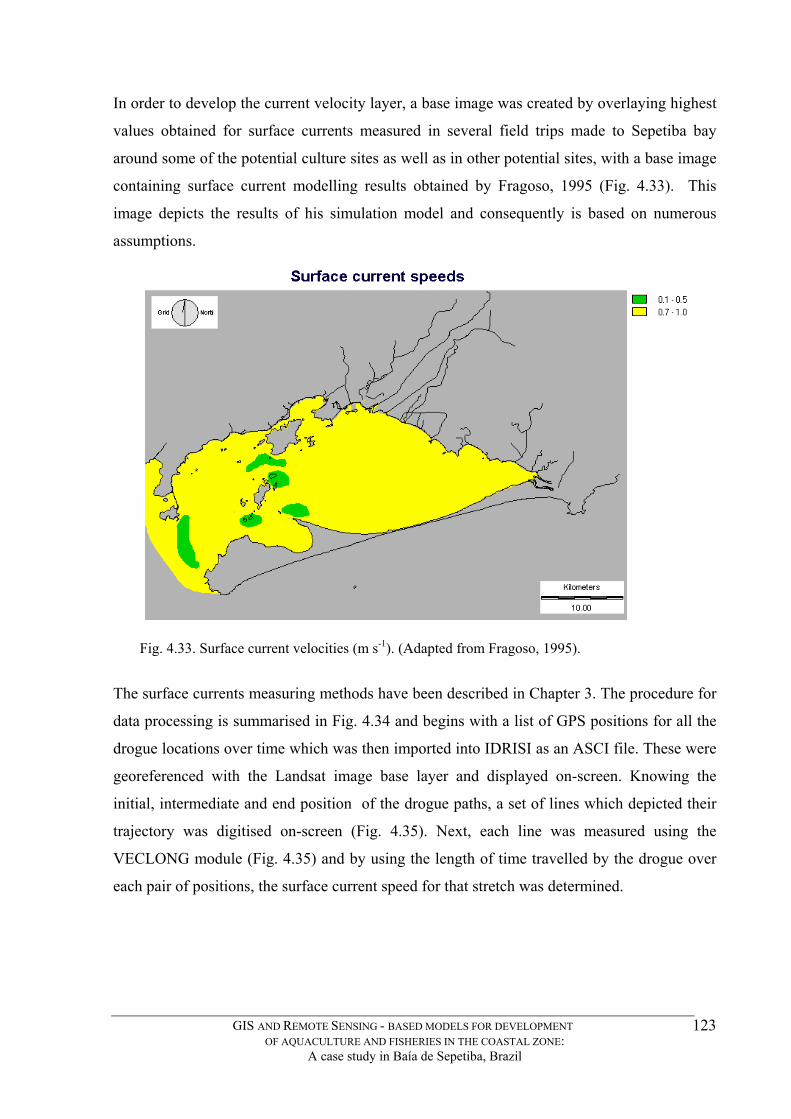
In order to develop the current velocity layer, a base image was created by overlaying highest

values obtained for surface currents measured in several field trips made to Sepetiba bay

around some of the potential culture sites as well as in other potential sites, with a base image

containing surface current modelling results obtained by Fragoso, 1995 (Fig. 4.33). This

image depicts the results of his simulation model and consequently is based on numerous

assumptions.

Fig. 4.33. Surface current velocities (m s-1). (Adapted from Fragoso, 1995).

The surface currents measuring methods have been described in Chapter 3. The procedure for

data processing is summarised in Fig. 4.34 and begins with a list of GPS positions for all the

drogue locations over time which was then imported into IDRISI as an ASCI file. These were

georeferenced with the Landsat image base layer and displayed on-screen. Knowing the

initial, intermediate and end position of the drogue paths, a set of lines which depicted their

trajectory was digitised on-screen (Fig. 4.35). Next, each line was measured using the

VECLONG module (Fig. 4.35) and by using the length of time travelled by the drogue over

each pair of positions, the surface current speed for that stretch was determined.



123

Fig. 4.34. Summary of current data entry into model.

In order to determine intermediate values between measured stretches (drogue runs), the

vector lines of the drogue paths were rasterised using the LINERAS module and then

converted into a point vector file using the POINTVEC module (Fig. 4.36). Using ASSIGN

current velocity values were assigned to the pixels along the drogue paths (Fig. 4.37). The

result of interpolating the current velocity values between each group of pixels along the

subsets of the drogue paths measured is shown in Fig. 4.38.

Finally, the subsets of all drogue study sections considered was compiled into a new image

CURRENTS (Fig 4.39) incorporating data from Fragoso’s study (Fig. 4.33) in an overlay

operation where the maximum value of current velocity of either image remained. This

resulting image (Fig. 4.39) was then reclassified according to the suitability scoring system

shown in Table 4.17 into Fig. 4.40 (CURENTOK), which was used in the final suitability

model.



124

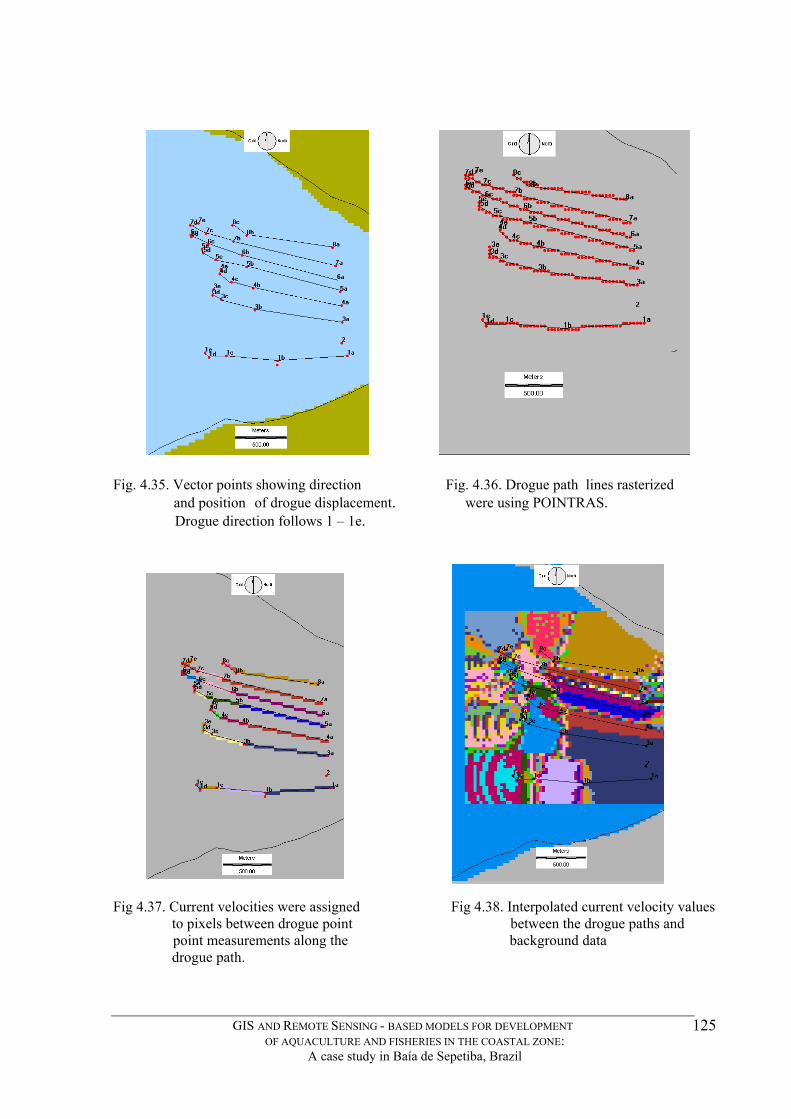
Fig. 4.35. Vector points showing direction Fig. 4.36. Drogue path lines rasterized

and position of drogue displacement. were using POINTRAS. Drogue direction follows 1 – 1e.

Fig 4.37. Current velocities were assigned Fig 4.38. Interpolated current velocity values to pixels between drogue point between the drogue paths and point measurements along the background data drogue path.



125

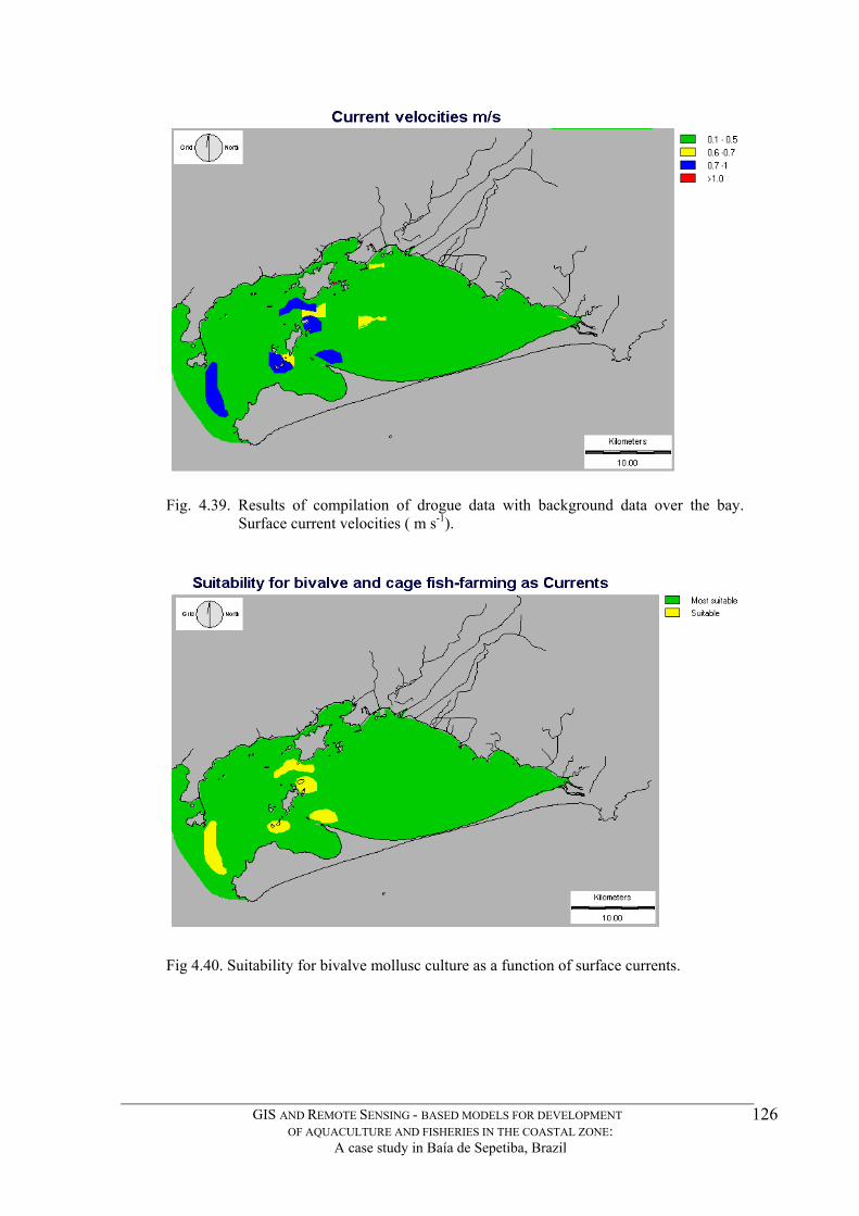
Fig. 4.39. Results of compilation of drogue data with background data over the bay. Surface current velocities ( m s-1).

Fig 4.40. Suitability for bivalve mollusc culture as a function of surface currents.



126

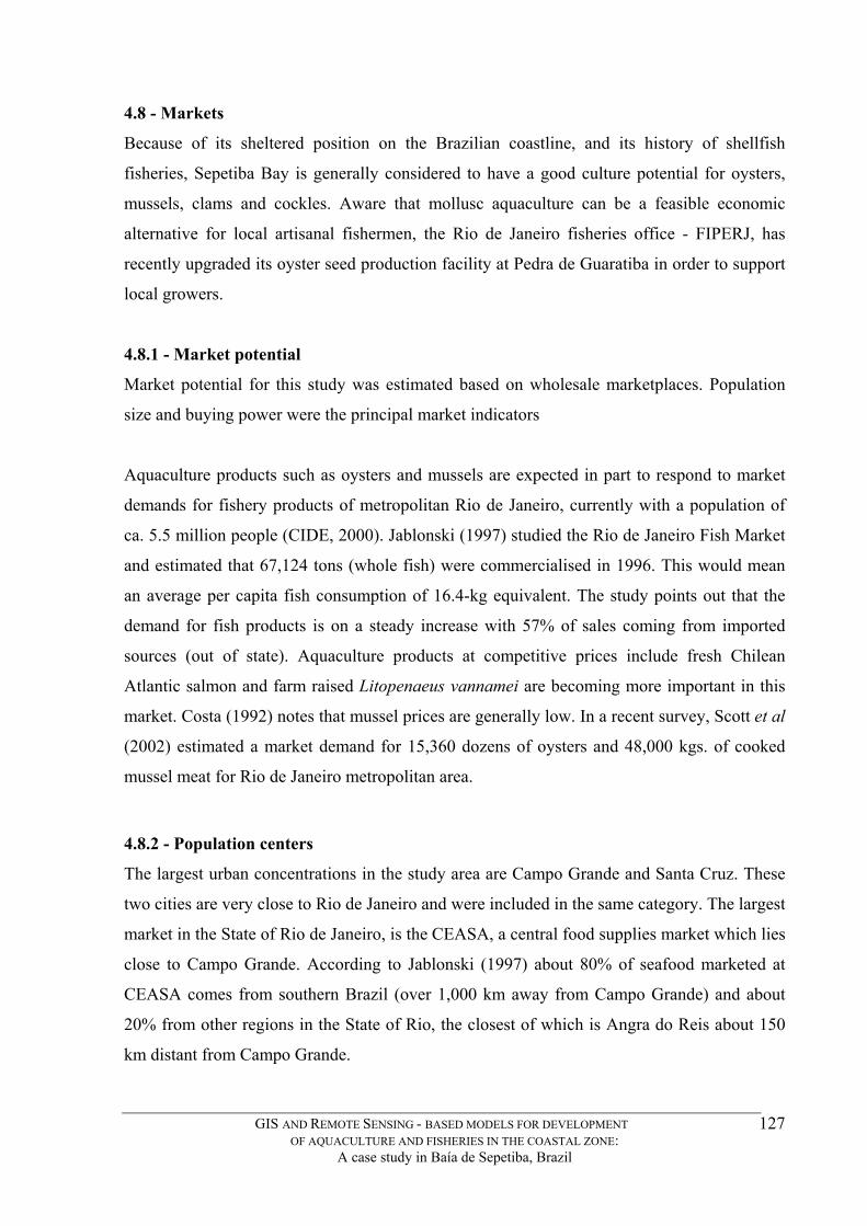
4.8 - Markets

Because of its sheltered position on the Brazilian coastline, and its history of shellfish

fisheries, Sepetiba Bay is generally considered to have a good culture potential for oysters,

mussels, clams and cockles. Aware that mollusc aquaculture can be a feasible economic

alternative for local artisanal fishermen, the Rio de Janeiro fisheries office - FIPERJ, has

recently upgraded its oyster seed production facility at Pedra de Guaratiba in order to support

local growers.

4.8.1 - Market potential

Market potential for this study was estimated based on wholesale marketplaces. Population

size and buying power were the principal market indicators

Aquaculture products such as oysters and mussels are expected in part to respond to market

demands for fishery products of metropolitan Rio de Janeiro, currently with a population of

ca. 5.5 million people (CIDE, 2000). Jablonski (1997) studied the Rio de Janeiro Fish Market

and estimated that 67,124 tons (whole fish) were commercialised in 1996. This would mean

an average per capita fish consumption of 16.4-kg equivalent. The study points out that the

demand for fish products is on a steady increase with 57% of sales coming from imported

sources (out of state). Aquaculture products at competitive prices include fresh Chilean

Atlantic salmon and farm raised Litopenaeus vannamei are becoming more important in this

market. Costa (1992) notes that mussel prices are generally low. In a recent survey, Scott et al

(2002) estimated a market demand for 15,360 dozens of oysters and 48,000 kgs. of cooked

mussel meat for Rio de Janeiro metropolitan area.

4.8.2 - Population centers

The largest urban concentrations in the study area are Campo Grande and Santa Cruz. These

two cities are very close to Rio de Janeiro and were included in the same category. The largest

market in the State of Rio de Janeiro, is the CEASA, a central food supplies market which lies

close to Campo Grande. According to Jablonski (1997) about 80% of seafood marketed at

CEASA comes from southern Brazil (over 1,000 km away from Campo Grande) and about

20% from other regions in the State of Rio, the closest of which is Angra do Reis about 150

km distant from Campo Grande.



127

Table 4.19 summarises the population characteristics of the main urban concentrations in the

study area. These towns were reclassified according to Table 4.20. Itaguaí and the towns of

Barra de Guaratiba and Pedra de Guaratiba were reclassified into the second most promising

markets. Coroa Grande and Sepetiba are the medium size coastal towns. There are several

other coastal towns with populations of less than 7,000 inhabitants, which were considered

individually as unsuitable markets for commercial aquaculture production distribution.

However, considering them as a group and taking into account seaside hotels and restaurants,

they represent a promising potential market. The reclassified image showing ongrowing site

suitability as a function of market potential is illustrated in Fig. 4.41.

Table 4.19. Population aspects of towns in the study area. (Adapted from CIDE, 2000).

City/town

Area (km2)

Population

Density

(People/ km2)

Annual growth rate (%)

Campo Grande 171.6 380,942 2,219.0 1.15 Santa Cruz 163.7 254,500 1,554.4 1.15 Guaratiba 151.7 60,774 400.5 1.15 Itaguaí 175 50,906 290.9 2.08 Mangaratiba 155 8,728 56.3 2.38 Coroa Grande 274 8,697 31.7 2.08 Vila Muriqui 53 4,346 82 2.38 Itacuruçá 23 3,543 154.0 2.38

Table 4.20. Suitability scoring for market potetial based on population density.

Interpretation Score Most Suitable Large markets, many retail outlets Population > 250,000

4

Suitable Average size market, good growth potential Population - 50,000 – 250,000

3

Moderately Suitable Marginal growth – limited market Population - 7,000 - 50,000

2

Unsuitable Small coastal towns – local street markets Population < 7,000

1



128

Fig 4.41. Site suitability for mollusc culture as a function of population density.

4.8.3 - Buying power

The local monthly minimum wage (MW) in Aug, 2002 was R$ 200 the equivalent of £41.30.

Table 4.21 summarises local statistics available which indicate the buying power of the

population in the study area. Five towns have 7.4 to 13.23 % of households earning between

£206.49 - £412.97 i.e. between five and ten minimum wages per month. Based on this

information, the towns in the study area were reclassified using the scoring system presented

in Table 4.22 (Fig. 4.42).

Table 4.21. Percentage of households earning 5 – 10 Minimum Wages (Adapted from SEMA, 1996).

City/town (rural and urban combined)

% of households with 5-10 MW.

Campo Grande 7.40- 13.23 Santa Cruz 7.40 - 13.23 Mangaratiba 7.40 - 13.23 Sepetiba 7.40 - 13.23 Vila Muriqui 7.40 - 13.23 Itacuruçá 5.09 -7.40 Itaguaí 5.09 -7.40 Guaratiba 5.09 -7.40 Coroa Grande 3.25 -5.09



129

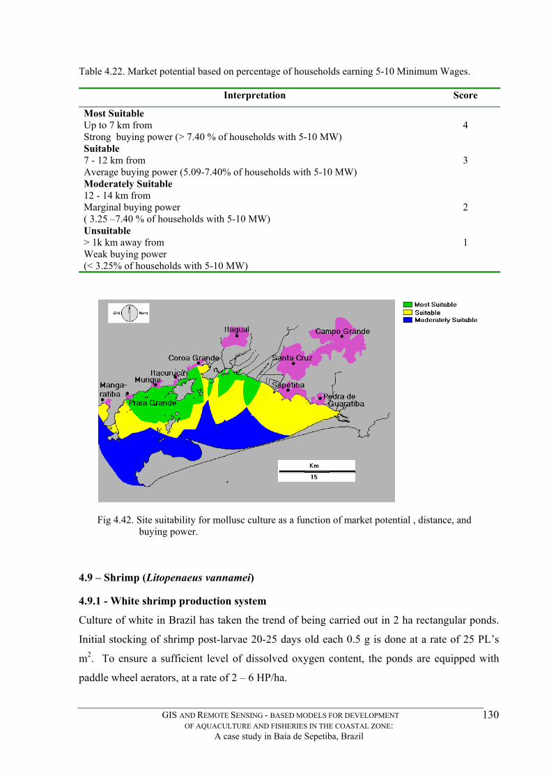
Table 4.22. Market potential based on percentage of households earning 5-10 Minimum Wages.


Most Suitable Up to 7 km from Strong buying power (> 7.40 % of households with 5-10 MW)

4

Suitable 7 - 12 km from Average buying power (5.09-7.40% of households with 5-10 MW)

3

Moderately Suitable 12 - 14 km from Marginal buying power ( 3.25 –7.40 % of households with 5-10 MW)

(< 3.25% of households with 5-10 MW)

2

Unsuitable > 1k km away from Weak buying power

1

Culture of white in Brazil has taken the trend of being carried out in 2 ha rectangular ponds.

Initial stocking of shrimp post-larvae 20-25 days old each 0.5 g is done at a rate of 25 PL’s

m ed oxygen content, the ponds are equipped with

paddle wheel aerators, at a rate of 2 – 6 HP/ha.

Fig 4.42. Site suitability for mollusc culture as a function of market potential , distance, and

buying power.

4.9 – Shrimp (Litopenaeus vannamei) 4.9.1 - White shrimp production system

2. To ensure a sufficient level of dissolv



130

These are usually activitaded when the DO level falls to 3 mgL-1, or biomass reaches 0.2 kg

m2). Pelleted feed is commonly used to feed growing shrimp. White shrimp culture cycle is

terminated at about 100-120 days, at which time each shrimp weighs approximately 12g.

Seawater exchange is provided by pumping from estuarine areas a rate of 15% of the pond

volume per day.

Table 4.23. Potential shrimp production.

White shrimp farming summary Units total Stocking density PLs25/m2 25 Cycle days 100 – 120

3,600

£ 5,940

Survival rate % 50-60 Average weight at sale g 12 Average production kg/ha/y-1 Farm gate price £/kg 1.65 Gross earnings per hectare/yr

Data based on Technical Report to IPP by Mathias, M.A. de C. (2003)

4.9.1.1 -Choice of Production Functions

Production functions for white shrimp production were developed from the database and

reclassified as suitability images. These include technical support, roads network, local

agriculture, shrimp seed availability, seawater sourcing, freshwater sourcing, soil quality

suitability, vegetation and land use analysis, climatic factors including: rainfall, air

temperature and a natural indicator of appropriate areas for shrimp farming. Although water

quality is most important for shrimp farming, it was not treated as a production factor in the

modelling used in this research because it was assumed that 1. all the seawater available in the

bay was adequate in terms of temperature (24 – 30 C) and salinity (7 – 32 ), 2. because the

intensive shrimp production model uses artificial aeration 4. Chlorophyll-a content is not very

relevant in this type of production since feeding come almost entirely from artificial feed

furnished to the shrimp and finally, 5. Water quality chemical parameters tend to be

controlled during ongrowing by frequent testing.

4.9.1.2 - Shrimp Farming Technical Support.

Shrimp aquaculture technical know-how is present in the study area in the form of the FIPERJ

fisheries research and extension lab and office.



131

The experts are familiar with all phases of shrimp culture and equipped to provide services

including diagnostics and feeding trials. Farms situated in a 5 km radius from the FIPERJ lab

(Fig 4.43) would be best placed since this is a distance short enough easily overcome even by

bicycle. Distances up to 30 km can easily be overcome by car or bus, and fall within the main

road network for the region. Distances over 30 km and less than 200 km, ares still within

feasible range of action, however locations over the 200 km limit would best be attended by

another expert support center.

Table 4..24. Suitability scoring for technical support availability.

Fig.4.43. Site suitability in function of distance from specialised aquaculture technical support.


Most Suitable Easy, quick access 0-5 km

4

Easy access by car or bus 5 - 30 km

3

30 – 200 km

2

> 200 km 1

Suitable

Moderately suitable Accessible, within the region’s main road network

Unsuitable



132

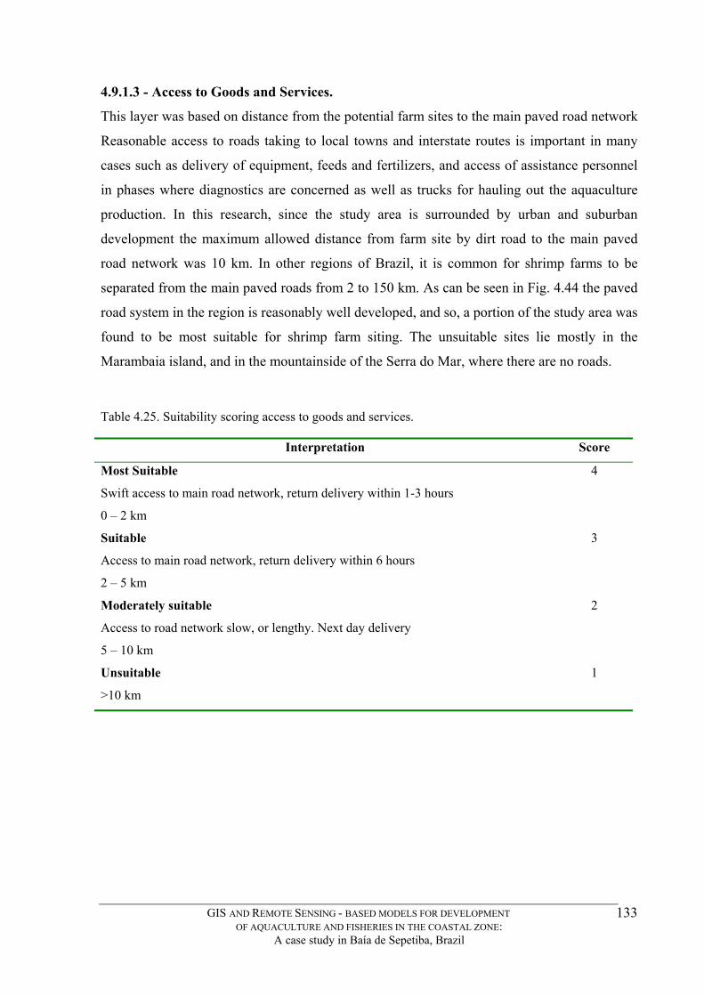
4.9.1.3 - Access to Goods and Services.

This layer was based on distance from the potential farm sites to the main paved road network

Reasonable access to roads taking to local towns and interstate routes is important in many

cases such as delivery of equipment, feeds and fertilizers, and access of assistance personnel

in phases where diagnostics are concerned as well as trucks for hauling out the aquaculture

production. In this research, since the study area is surrounded by urban and suburban

development the maximum allowed distance from farm site by dirt road to the main paved

road network was 10 km. In other regions of Brazil, it is common for shrimp farms to be

separated from the main paved roads from 2 to 150 km. As can be seen in Fig. 4.44 the paved

road system in the region is reasonably well developed, and so, a portion of the study area was

found to be most suitable for shrimp farm siting. The unsuitable sites lie mostly in the

Marambaia island, and in the mountainside of the Serra do Mar, where there are no roads.

Table 4.25. Suitability scoring access to goods and services.


Most Suitable

Swift access to main road network, return delivery within 1-3 hours

0 – 2 km

4

Suitable

Access to main road network, return delivery within 6 hours

2

2 – 5 km

3

Moderately suitable

Access to road network slow, or lengthy. Next day delivery

5 – 10 km

Unsuitable

>10 km

1



133

Fig 4.44. Site suitability in function of access to goods and services in the region. 4.9.1.4 - Land Availability.

Farmland and semi-intensive agriculture operations in the area were used as an important

indication of land availability and suitability for shrimp pond construction. This layer was

built based on ground truth information collected in the database development phase of this

research and interpretation of the Landsat image of a 354 RGB colour composite. As the

study area is experiences steady development of urban development, a buffer zone of 500 m

around the agriculture coverage was considered as the maximum distance feasible to be

maintained between a shrimp farm activity and suburban development. This was based on

interview with two shrimp farm managers and their experience. Three potential farm

development areas are shown in Fig. 4.45, the largest of which is around the Itaguaí area,

known for its tradition in agriculture mainly cassava, guava, sugarcane and coconut

plantations.

Table 4.26. Suitability scoring for land availability.

Interpretation Score Most Suitable Seasonal agriculture plots, pastures, farmland 0 – 0.5 km

4

Unsuitable suburban development, urban areas, forestry > 0.5 km

1



134

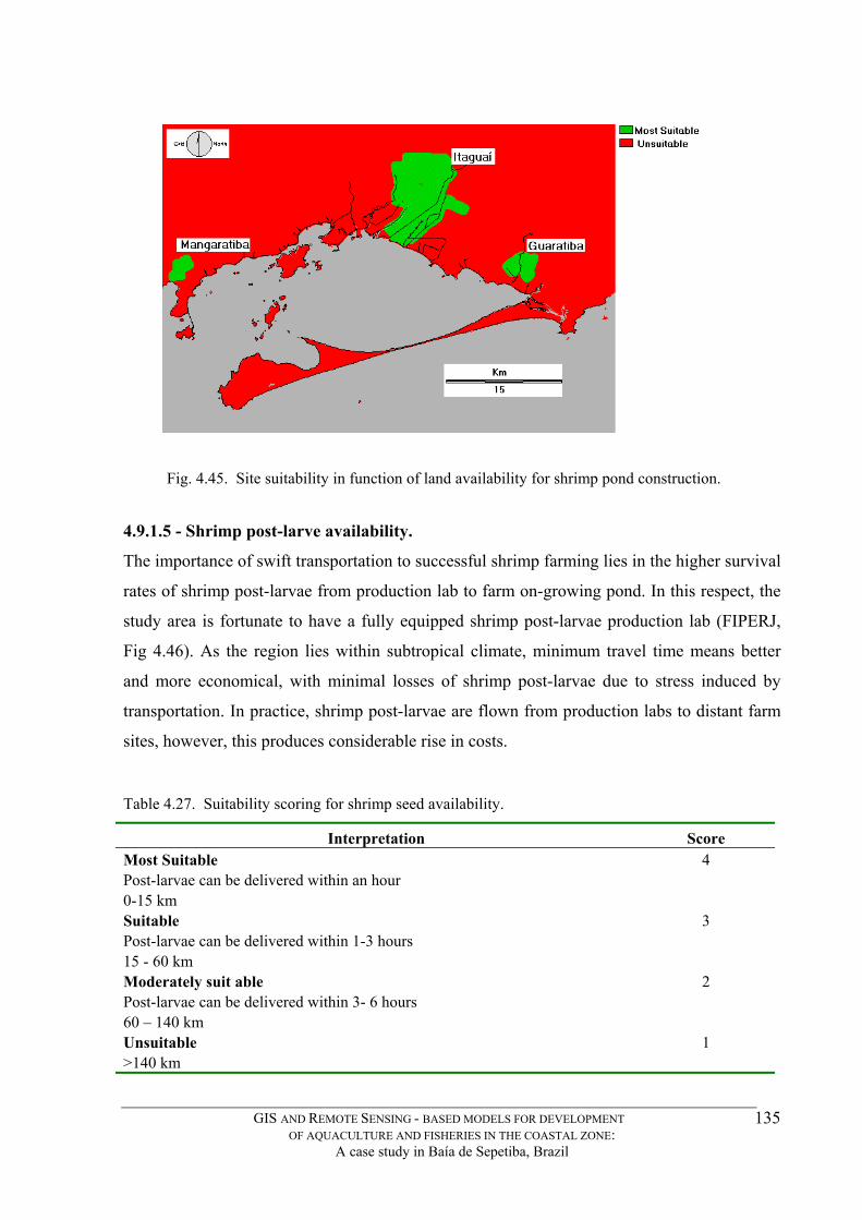
Fig. 4.45. Site suitability in function of land availability for shrimp pond construction. 4.9.1.5 - Shrimp post-larve availability.

The importance of swift transportation to successful shrimp farming lies in the higher survival

rates of shrimp post-larvae from production lab to farm on-growing pond. In this respect, the

study area is fortunate to have a fully equipped shrimp post-larvae production lab (FIPERJ,

Fig 4.46). As the region lies within subtropical climate, minimum travel time means better

and more economical, with minimal losses of shrimp post-larvae due to stress induced by

transportation. In practice, shrimp post-larvae are flown from production labs to distant farm

sites, however, this produces considerable rise in costs.

Table 4.27. Suitability scoring for shrimp seed availability.

Interpretation Score Most Suitable Post-larvae can be delivered within an hour 0-15 km

4

Suitable Post-larvae can be delivered within 1-3 hours 15 - 60 km

3

Moderately suit able Post-larvae can be delivered within 3- 6 hours 60 – 140 km

2

Unsuitable >140 km

1



135


Fig 4.46. Site suitability in function of distance from shrimp post-larvae production center. 4.9.1.6 - Marine water availability.

The basic pre-requisite for successful rearing of peaneid shrimps is the availability of

seawater. Sepetiba bay’s continental shoreline extends for approximately 55 km. In practice,

most shrimp farms tend to install their seawater pumping stations along the coast, or very

close to it. However, many farms do site their pumping stations within the intertidal range,

sometimes upstream in estuarine areas. In cases where coastal lands have a favourable

topography, seawater can be distributed via a feeder canal to ponds considerably distant from

the shoreline. In this study, a maximum distance from the shoreline of 7 km was adopted as a

result of field verification in the Guaratiba region, where mangrove vegetation and regime

was found up to 7 km distant from the main coastline. Thus, potentially seawater could be

abstracted from mangrove canals distant from the seashore. Figure 4.47 shows the suitabilty

of the study area in function of distance from the coastline as a source for abstractin seawater

for pond filling.

Table 4.28. Suitability scoring for seawater intake availability .



136

Most Suitable Lowest cost for seawater abstraction and distribution 0 – 1 km

4

Suitable Potentially higher costs due to more sofisticated pumping station and increase in equipment 1 – 2.5 km

3

Moderately suitable Maximum intertidal range found at Guaratiba 2.5 – 7 km

2

Unsuitable > 7 km

1

Fig. 4.47. Suitability in function of seawater availablity for filling shrimp ponds. 4.9.1.7 - Freshwater availability.

Freshwater sources are important for maintaining shrimp pondwater quality in terms of

salinity. When possible, shrimp farms will have a pumping station or a sluice gate mecanism

in local freshwater courses in order to provide freshwater intake for mixing with seawater in a

‘mixing canal’. This way, adequate salinity is obtained for further distribution to ongrowing

pond water intakes. To develop a freshwater availability suitability layer, a vector file

describing the main rivers and canals present in Sepetiba bay was digitised, rasterised, and

applied a distance algorythm. Subsequently it was reclassified by the criteria shown in Table

4.29. The volumes of freshwater available from these sources vary considerably from 17m3s-1

for the Rio Piraquê to 342 m3s-1 for the Guandú canal (Figure 4.48). However, this

information was not used to further reclassify the amount of available freshwater to potential

shrimp farms in the area.. These freshwater sources in the study area could also be reclassified

in function of their suitability as concerns water temperature. For example, the Mazomba river

which descends from a closeby mountain range approximately 400 m high has cooler waters

than the Itaguaí and Itá rivers which travel over lowland regions for several kilometers.



137

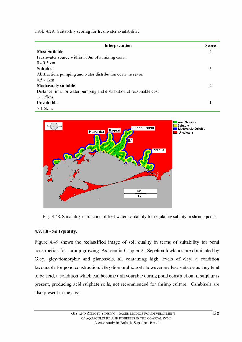
Table 4.29. Suitability scoring for freshwater availability.

Interpretation Score Most Suitable Freshwater source within 500m of a mixing canal. 0 - 0.5 km

4

Suitable Abstraction, pumping and water distribution costs increase. 0.5 - 1km

3

Moderately suitable Distance limit for water pumping and distribution at reasonable cost 1- 1.5km

2

Unsuitable > 1.5km.

1

Fig. 4.48. Suitability in function of freshwater availablity for regulating salinity in shrimp ponds. 4.9.1.8 - Soil quality.

Figure 4.49 shows the reclassified image of soil quality in terms of suitability for pond

construction for shrimp growing. As seen in Chapter 2., Sepetiba lowlands are dominated by

Gley, gley-tiomorphic and planossols, all containing high levels of clay, a condition

favourable for pond construction. Gley-tiomorphic soils however are less suitable as they tend

to be acid, a condition which can become unfavourable during pond construction, if sulphur is

present, producing acid sulphate soils, not recommended for shrimp culture. Cambisols are

also present in the area.



138

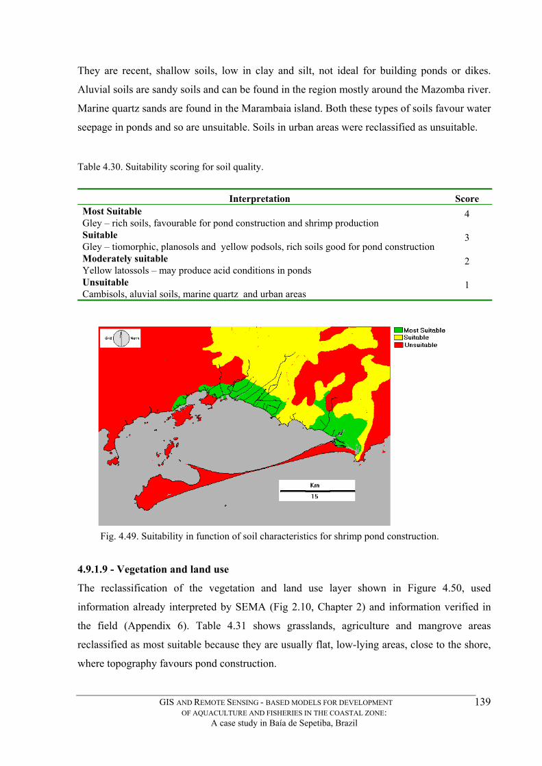
They are recent, shallow soils, low in clay and silt, not ideal for building ponds or dikes.

Aluvial soils are sandy soils and can be found in the region mostly around the Mazomba river.

Marine quartz sands are found in the Marambaia island. Both these types of soils favour water

seepage in ponds and so are unsuitable. Soils in urban areas were reclassified as unsuitable.

Table 4.30. Suitability scoring for soil quality.

Interpretation Score Most Suitable Gley – rich soils, favourable for pond construction and shrimp production

4

Suitable Gley – tiomorphic, planosols and yellow podsols, rich soils good for pond construction

3

Moderately suitable Yellow latossols – may produce acid conditions in ponds

2

Unsuitable Cambisols, aluvial soils, marine quartz and urban areas

1

Fig. 4.49. Suitability in function of soil characteristics for shrimp pond construction.

The reclassification of the vegetation and land use layer shown in Figure 4.50, used

information already interpreted by SEMA (Fig 2.10, Chapter 2) and information verified in

the field (Appendix 6). Table 4.31 shows grasslands, agriculture and mangrove areas

reclassified as most suitable because they are usually flat, low-lying areas, close to the shore,

where topography favours pond construction.

4.9.1.9 - Vegetation and land use



139

Waterlogged were considered suitable, but represent higher construction costs, and indicate

potentially acid soil conditions. The study area also has many forests some of which are on

hilly terrain as is typical in the region (coastal Atlantic rainforest) others which are eucalyptus

logging areas. Restinga (coastal sandy area vegetation) such as that present on Marambaia

island and urban areas were considered unsuitable because of high seepage rates or

unavailability.


Table 4.31. Suitability scoring for vegetation and land use.

Most Suitable Easily transformed into shrimp ponds at low costs. grasslands, agriculture, mangroves

4

Drainage of terrain can increase pond construction costs waterlogged soils Moderately suitable 2

1

Suitable 3

Unsuitable – forests, restinga, urban areas

Fig. 4.50. in function of vegetation cover and land use.

4.9.1.10 - Rainfall.

As can be seen in Figure 4.51, a large portion of the study area has rainfall values between

1000-2000mm yr

Suitability

-1.



140

These were considered suitable as this range can replenish the freshwater sources in the

catchment area, and support maintenance of salinity in the shrimp ponds either directly

through rainfall over the pond surface, or alternatively by contributing to the river sources

which in turn are used by the farm by means of pumping or diverting water courses. Areas

with yearly rainfall values over 2000 mm were reclassified as unsuitable because of the

likelihood of flooding and damages to pond dikes which can cause loss of production. Some

of these areas are located at the base of the hills in the Itacuruçá - Muriquí region, by the sea.

Areas with rainfall values under 1000 mm yr , are associated with temperature regime which

contributes towards undesirable salinisation of pondwater, leading to shrimp stress and hence

lower productivity. Large areas of the study area were re-classified as suitable to most

suitable. Air humidity in most of the area is around 85%.

-1

Table 4.32. Suitability scoring for rainfall

Interpretation Score Most Suitable – 4 1000- 1200 mm – rainfall just covers evaporation Suitable 1200 – 1600 mm

3

tendency to lower salinity in ponds

2

1000 mm > 2000 mm Ponds will need replenishment or may end up flooding

Moderately suitable 1600 – 2000

Unsuitable 1

Fig. 4.51. Suitability in function of rainfall.



141

4.9.1.11 - Air temperature

Air temperature was used as an indication of water temperature suitability for shrimp culture.

Although Litopenaeus vannamei grows in a wide temperature range, optimal culture

conditions which allow three on-growing cycles per year, such as found in northeastern Brazil

are on avearage 27 C year round. The reclassication scheme adopted in Table 4.33 was

arbitrated with an aquaculture expert and shrimp farm manager with many years hands on

experience in shrimp farming.

Table 4.33. Suitability scoring for air temperature ( C). o

Interpretation Score Most Suitable Best growing conditions > 24.0

4

Suitable 23.5 – 24,0 3 Moderately suitable 21.5 - 23.5 2 Unsuitable < 21.5 1

Fig. 4.52. Site suitability in function of air temperature. 4.9.1.12 - Climate

Figure 4.53 shows the reclassification results of Figure 2.6 which describes the climatic types

for the study area. Warm tropical climate is favourable for white shrimp culture.



142

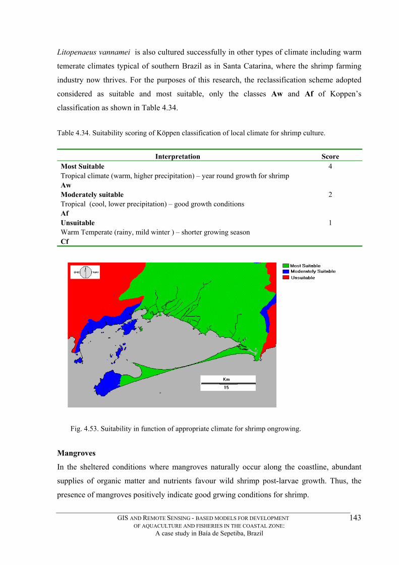
Litopenaeus vannamei is also cultured successfully in other types of climate including warm

temerate climates typical of southern Brazil as in Santa Catarina, where the shrimp farming

industry now thrives. For the purposes of this research, the reclassification scheme adopted

considered as suitable and most suitable, only the classes Aw and Af of Koppen’s

classification as shown in Table 4.34.

Table 4.34. Suitability scoring of Köppen classification of local climate for shrimp culture.

Interpretation Score Most Suitable Tropical climate (warm, higher precipitation) – year round growth for shrimp Aw

4

Moderately suitable Tropical (cool, lower precipitation) – good growth conditions Af

2

Unsuitable 1 Warm Temperate (rainy, mild winter ) – shorter growing season Cf

In the sheltered conditions where mangroves naturally occur along the coastline, abundant

supplies of organic matter and nutrients favour wild shrimp post-larvae growth. Thus, the

presence of mangroves positively indicate good grwing conditions for shrimp.

Fig. 4.53. Suitability in function of appropriate climate for shrimp ongrowing. Mangroves



143

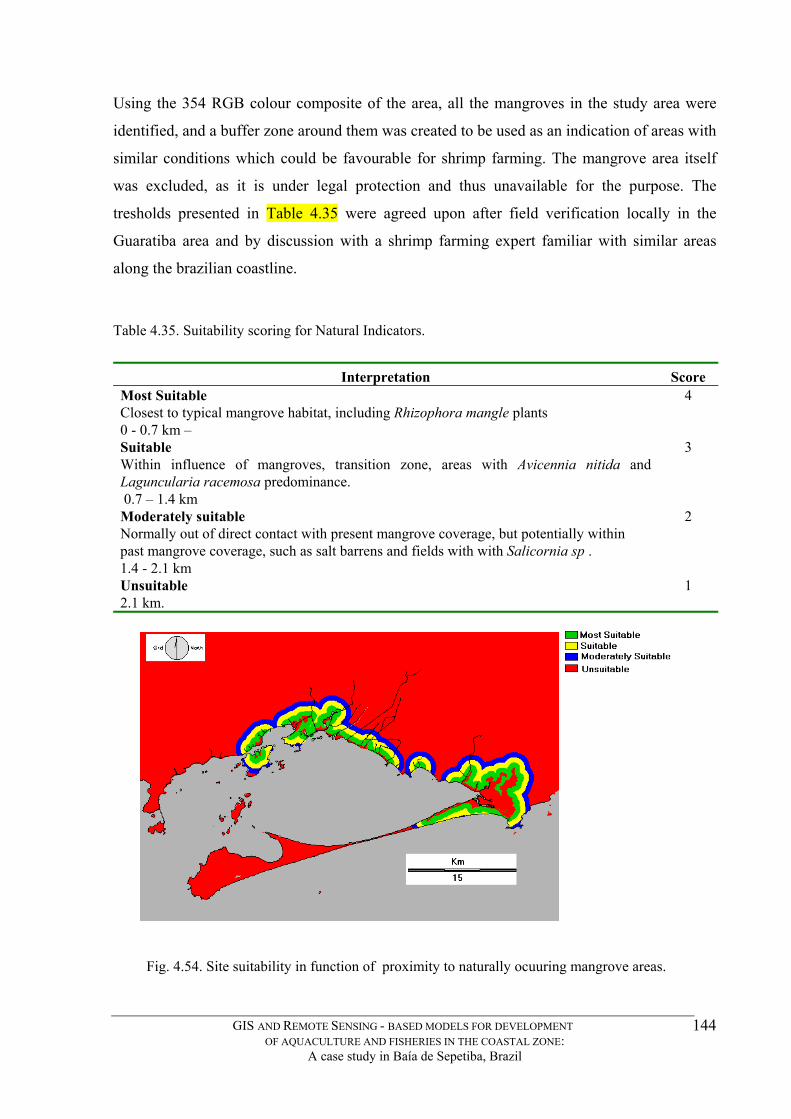
Using the 354 RGB colour composite of the area, all the mangroves in the study area were

identified, and a buffer zone around them was created to be used as an indication of areas with

similar conditions which could be favourable for shrimp farming. The mangrove area itself

was excluded, as it is under legal protection and thus unavailable for the purpose. The

tresholds presented in Table 4.35 were agreed upon after field verification locally in the

Guaratiba area and by discussion with a shrimp farming expert familiar with similar areas

along the brazilian coastline.

Table 4.35. Suitability scoring for Natural Indicators.

Interpretation Score Most Suitable Closest to typical mangrove habitat, including Rhizophora mangle plants 0 - 0.7 km –

4

Within influence of mangroves, transition zone, areas with Avicennia nitida and Laguncularia racemosa predominance. 0.7 – 1.4 km

3

Moderately suitable Normally out of direct contact with present mangrove coverage, but potentially within past mangrove coverage, such as salt barrens and fields with with Salicornia sp . 1.4 - 2.1 km

2

Unsuitable 2.1 km.

Fig. 4.54. Site suitability in function of proximity to naturally ocuuring mangrove areas.

Suitable

1



144

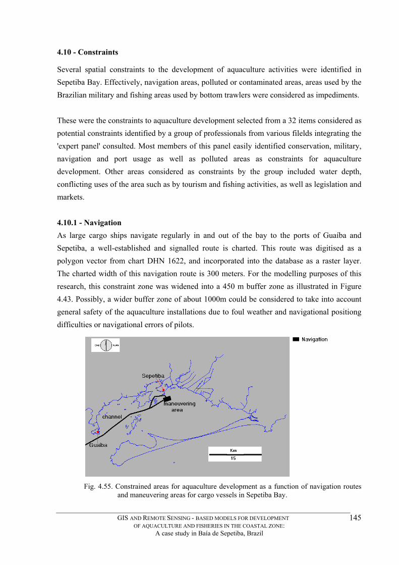
4.10 - Constraints

Several spatial constraints to the development of aquaculture activities were identified in Sepetiba Bay. Effectively, navigation areas, polluted or contaminated areas, areas used by the Brazilian military and fishing areas used by bottom trawlers were considered as impediments. These were the constraints to aquaculture development selected from a 32 items considered as potential constraints identified by a group of professionals from various filelds integrating the 'expert panel' consulted. Most members of this panel easily identified conservation, military, navigation and port usage as well as polluted areas as constraints for aquaculture development. Other areas considered as constraints by the group included water depth, conflicting uses of the area such as by tourism and fishing activities, as well as legislation and markets. 4.10.1 - Navigation As large cargo ships navigate regularly in and out of the bay to the ports of Guaíba and Sepetiba, a well-established and signalled route is charted. This route was digitised as a polygon vector from chart DHN 1622, and incorporated into the database as a raster layer. The charted width of this navigation route is 300 meters. For the modelling purposes of this research, this constraint zone was widened into a 450 m buffer zone as illustrated in Figure 4.43. Possibly, a wider buffer zone of about 1000m could be considered to take into account general safety of the aquaculture installations due to foul weather and navigational positiong difficulties or navigational errors of pilots.

Fig. 4.55. Constrained areas for aquaculture development as a function of navigation routes and maneuvering areas for cargo vessels in Sepetiba Bay.



145

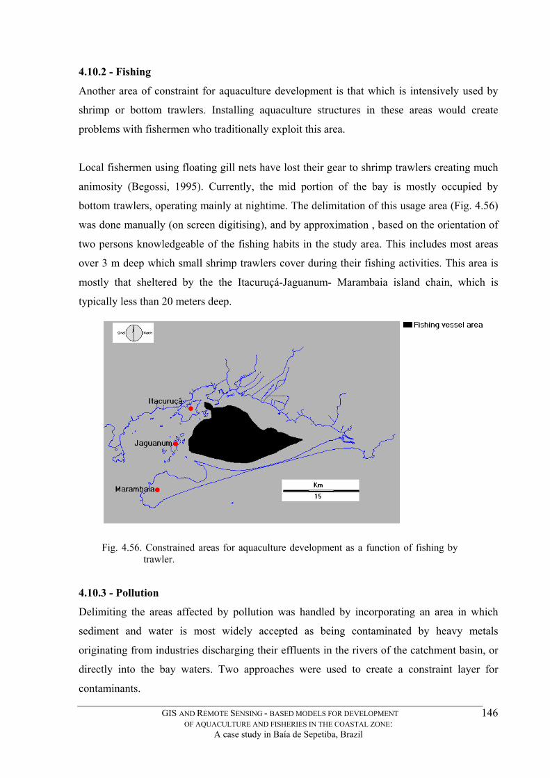
4.10.2 - Fishing

Fig. 4.56. Constrained areas for aquaculture development as a function of fishing by trawler.

Another area of constraint for aquaculture development is that which is intensively used by

shrimp or bottom trawlers. Installing aquaculture structures in these areas would create

problems with fishermen who traditionally exploit this area.

Local fishermen using floating gill nets have lost their gear to shrimp trawlers creating much

animosity (Begossi, 1995). Currently, the mid portion of the bay is mostly occupied by

bottom trawlers, operating mainly at nightime. The delimitation of this usage area (Fig. 4.56)

was done manually (on screen digitising), and by approximation , based on the orientation of

two persons knowledgeable of the fishing habits in the study area. This includes most areas

over 3 m deep which small shrimp trawlers cover during their fishing activities. This area is

mostly that sheltered by the the Itacuruçá-Jaguanum- Marambaia island chain, which is

typically less than 20 meters deep.

4.10.3 - Pollution

Delimiting the areas affected by pollution was handled by incorporating an area in which

sediment and water is most widely accepted as being contaminated by heavy metals

originating from industries discharging their effluents in the rivers of the catchment basin, or

directly into the bay waters. Two approaches were used to create a constraint layer for

contaminants.



146

Firstly, the main point sources of contamination were established, based on the main river

outflows (Canal de São Francisco and the Canal do Guandú (Fig. 4.57), and point sources

such as the Ingá zinc production facility. From these points, Since few studies that precisely

map the contamination effects of the pollution above mentioned an arbitrary buffer zone

conisisting of a 7 km radius from the point sources was drawn., based on an independent

survey carried out by ALERJ (1996). This 7 km radius buffer zone is a tentative way of

avoiding contaminated waters and their direct negative effects on bivalve growth such as shell

deformations in oysters by excess Cadmium and Zinc absorption.

Fig. 4.57. Constrained areas for aquaculture development as a function of point pollution sources.

Secondly, based on a survey undertaken by FEEMA/GTZ (1997) where bottom sediments

from across the bay were analysed for zinc concentration, a vector point file was created

indicating the geographical position of each sampling station. This file was converted to a

values file with the equivalent concentration of Zinc (µL ). This vector file was then

interpolated in order to produce an estimated concentration range layer over the bay area (Fig.

4.58).

-1

The general consensus of technicians, consultants and extension officers is that this area (Fig.

4.57) is subject to pollution effects and expected to be least recommended for aquaculture

implementation. It would also be very difficult to obtain development approval.



147

Fig. 4.58. Zinc concentration in bottom sediments.

-1

Fig. 4.59. Constrained areas for aquaculture development in function of pollution or contamination of bottom sediments.

Based on the 1977 resolution of the Brazilian Environment Ministry (SEMA) which allows a

maximum level for Zinc in sediments of coastal environments, all areas where the

interpolation procedure resulted in values of 800 µL or more were reclassified into a

constraint zone, which was merged (OVERLAY) with those areas considered unsuitable by

technicians due to proximity to point pollution sources (Fig. 4.45) resulting in Fig. 4.59.



148

4.10.4 - Military Use

The Brazilian military maintain a target shooting range on the Restinga de Marambaia, and so

have a security exclusion area charted on admiralty chart DHN 1622 from which this area was

digitised and imported into the GIS database (Fig. 4.60). Fishing vessels are allowed passage

but must not stop. It is unlikely that the military authorities will allow aquaculture

installations or permits in this exercise area. Table 4.23 summarises the constraints found for

aquaculture development detected in Sepetiba Bay.

Fig. 4.60. Constrained area for aquaculture development due to military restriction..

4.10.5 – Total Constraints

Mussel farming. Figure 4.61 shows the total constrained for installation of mussel longlines.

This includes all of the previous constraint layers as well as a constraint layer for depths less

than 3 m, as this was considered too shallow for installation of the longline achoring system.

The study area in the bay was found to contain 18,759 ha suitable for modelling for mussel

culture (34.5 % of the study area).



149

Fig. 4.61. Total constrained area for mussel culture.

Oyster farming. Figure 4.62 shows the total constrained area for installation of intertidal

oyster culture. This includes all of the constraint layers previously described as well as a

constraint layer for depths greater than 3 m, considered unsuitable for installation of intertidal

rack system for mangrove oyster cultivation. The study area in the bay was found to 2,407 ha

suitable for modelling for mangrove oysters culture (4.43 % of the study area).

Fig. 4.62. Total constrained area for oyster culture.



150

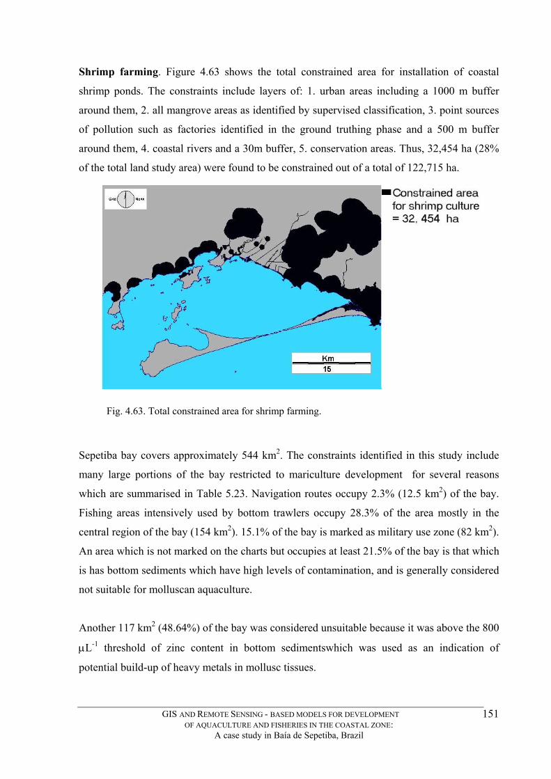
Shrimp farming. Figure 4.63 shows the total constrained area for installation of coastal

shrimp ponds. The constraints include layers of: 1. urban areas including a 1000 m buffer

around them, 2. all mangrove areas as identified by supervised classification, 3. point sources

of pollution such as factories identified in the ground truthing phase and a 500 m buffer

around them, 4. coastal rivers and a 30m buffer, 5. conservation areas. Thus, 32,454 ha (28%

of the total land study area) were found to be constrained out of a total of 122,715 ha.

Sepetiba bay covers approximately 544 km

many large portions of the bay restricted to mariculture development for several reasons

which are summarised in Table 5.23. Navigation routes occupy 2.3% (12.5 km

Fishing areas intensively used by bottom trawlers occupy 28.3% of the area mostly in the

central region of the bay (154 km arked as military use zone (82 km

An area which is not marked on the charts but occupies at least 21.5% of the bay is that which

is has bottom sediments which have high levels of contamination, and is generally considered

not suitable for molluscan aquaculture.

Fig. 4.63. Total constrained area for shrimp farming.

2. The constraints identified in this study include

2) of the bay.

2). 15.1% of the bay is m 2).

Another 117 km (48.64%) of the bay was considered unsuitable because it was above the 800

µL threshold of zinc content in bottom sedimentswhich was used as an indication of

potential build-up of heavy metals in mollusc tissues.

2

-1



151

With the exclusion of all these restricted areas, this study identified aproximately 2.9% (1,570

ha) areas classified as with Most Suitable potential for mussel culture production (Fig. 5.11),

and another 7.3% (576 hectares) for mangrove oyster (Fig. 5.15). A similar analysis was not

performed for all the constrained areas for land-based shrimp culture in ponds.

Table 4.36. Constraints for aquaculture usage detected in Sepetiba Bay.

Area hectares % 0f the bay Total area of the bay 54,396.54 100.0 Water and sediment pollution or contamination 11,709.54 21.5 Usage by small fishing trawlers 15,424.37 28.4 Usage by commercial navigation

Areas with Zinc contaminated bottom sediments ( > 800 µg

total impeded areas (excluding depth constraint)

1,218.95 2.2 Usage by military 8,191.08 15.1

-1 Zn) 26,461.08 48.6 Areas deeper than 3m (oyster culture system constraint) 42,224.85 77.6 Areas between 0 - 3m (mussel culture system constraint) 12,171.69 46.0

33,391.44

61.4



152

CHAPTER 5.

5.1 - Model design

The decision making process was assisted by using Multi-Criteria Evaluation (MCE) in order

to find the most suitable sites for aquaculture development. In this way, sets of similar criteria

were combined to achieve intermediary resulting images for each sub-model, which were

once again combined in a single and final MCE to achieve the specific objective of

identifying all suitable areas.

In order to use the MCE module of IDRISI, a set of relative weights for each criterion in the

sub-models was developed. This was accomplished by using the WEIGHT module of

IDRISI. Weights were developed by carrying out a series of pairwise comparisons of the

relative importance of each criterion being evaluated in each submodel.

MODEL DESIGN

The primary model structure used in this research was based on a review of primary literature,

followed by an attempt to determine relative weights for each of the production functions in

the identified sub-models. Following exploratory modelling, the approach initially adopted

was to canvas a wider and broad-based audience of professionals, collecting their impressions

by means of a questionnaire. This was further developed by focusing on a smaller science-

based group of professionals specialised in aquaculture, rating those culture related issues

pertinent to the principal sub-model (i.e. water quality, basis for organism survival, growth

and socio-economic aspects of aquaculture development).

The natural range of values for each of the production functions important for aquaculture

development in Sepetiba Bay, and the local set of constraints present, were developed into

raster images as described in the previous chapter. These images were combined logically into

four sub-models: Water Quality, Infrastructure, Physical Factors and Markets, as illustrated in

Figures 5.3 and 5.4. Sub-models were subsequently adjusted with a composite constraint

image, including all types of development impediments encountered, the final objective being

to arrive at an image depicting the best possible sites for aquaculture development in Sepetiba

Bay.



153

These pairwise comparisons were then analysed to produce a set of weights that sum to 1.

The factors and their resulting weights were used as input for the MCE module for a

weighted linear combination. The procedure by which the weights were developed is

described below and follows the logic developed by Saaty, 1977 under the Analytical

Hierarchy Process (AHP).

The weights used in all sub-models were derived by analysing trends of weights attributed by

a range of professionals from different areas related to aquaculture. In a first phase, a simple

questionnaire was applied to a group consisting of 19 professionals from the Economics,

Urban Planning, Aquaculture consultancy, Fisheries research and extension, Biology and

Environmental Sciences areas. Many of these were fellow lecturers and invited guests

assembled at Universidade Santa Úrsula for a Workshop held on 26/11/1997. All members of

the group were familiar with the general area of Sepetiba. The group was considered as a

local ‘expert panel’.

The purpose of the questionnaire was explained as being a means to collect impressions and

determine ranks for aquaculture variables in a site selection process using GIS. The questions

asked of the participants were as follows:

1. Name

5. Describe how your work is accomplished.

Before the participants answered the questionnaire, and in order to level out the general

understanding of the group on the issue, an introductory, brief explanation about mariculture

was given. Broadly, it was described as being “an activity which utilises the marine/coastal

environment to grow food organisms such as oysters, mussels, shrimp or fish under controlled

conditions”.

2. Profession (As in: Architect, Biologist, Economist, Engineer…) 3. Area of expertise (largest know-how by training ) 4. Area of specific daily action (e.g. lecturer, grower, consultant, extension agent,

municipal administrator, researcher…)

6. What issues you consider as being Constraints to the development of aquaculture? 7. What issues you consider as being Production or Limiting Factors to the

development of aquaculture?



154

Also that aquaculture is practised in coastal sites around such as protected bays where

shellfish including mussels and oysters growing on floating structures or alternatively on

fixed racks situated in the intertidal zone, as well as fish in floating sea cages or shrimp in

coastal ponds. For this type of production to occur, the group was advised that some issues are

restrictive to the activity in one way or another, (constraints) and they should be listed.

The basic distinction between constraints and limiting factors (production functions) was

made. Constraints were defined as those factors which due to some 'higher force' could

actually impede the development of the activity as for example in the case of a specific

legislation ruling out use of an area for the purpose, or in the case of heavy pollution of the

environment.

Limiting factors (production functions or variables) were defined as those variables which

could increase or diminish production, as a function of their intensity, such as in the case of

water temperature or salinity which affect the physiology of an organism, or alternatively

natural availability of foodstuffs affecting growth. The group was asked to list those factors

which could increase, or reduce the biological production of farmed organisms.

A brief description of the geographic study area, western Rio de Janeiro and specifically

Sepetiba Bay, was given.

The complete list of all participants, their occupation and area of expertise is found in

Appendix 9. With all of the participants in the meeting room, the questionnaire session

followed, lasting for about two hours, where each person independently noted down what

factors he/she considered as being relative to 'production function variables' or 'constraints to

aquaculture development'. The complete list obtained is shown in Appendix 10. Once the

individual listing of production function variables was completed, they were asked to group

production function variables into similar function groups, in an attempt to identify potential

sub-models, and finally, to score each variable in the sub-models using AHP.



155

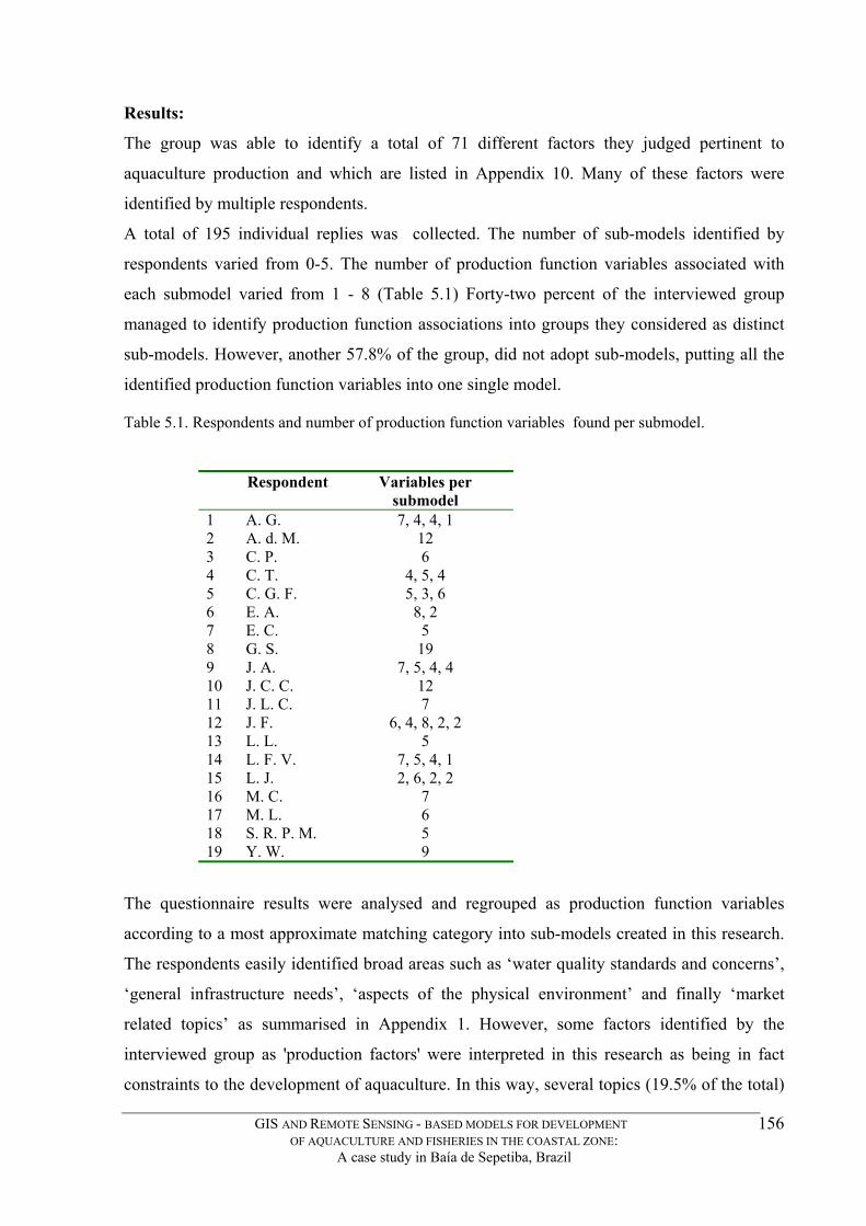
Results:

A total of 195 individual replies was collected. The number of sub-models identified by

respondents varied from 0-5. The number of production function variables associated with

each submodel varied from 1 - 8 (Table 5.1) Forty-two percent of the interviewed group

managed to identify production function associations into groups they considered as distinct

sub-models. However, another 57.8% of the group, did not adopt sub-models, putting all the

identified production function variables into one single model.

Table 5.1. Respondents and number of production function variables found per submodel.

Respondent Variables per submodel

1 A. G. 7, 4, 4, 1 2 A. d. M.

6 4, 5, 4 5, 3, 6

8, 2

9 J. A. J. C. C. 12 J. L. C. J. F.

5 14 15

7 17 18

Y. W.

12 3 C. P. 4 C. T. 5 C. G. F.

The group was able to identify a total of 71 different factors they judged pertinent to

aquaculture production and which are listed in Appendix 10. Many of these factors were

identified by multiple respondents.

6 E. A. 7 E. C. 5 8 G. S. 19

7, 5, 4, 4 10 11 7 12 6, 4, 8, 2, 2 13 L. L.

L. F. V. 7, 5, 4, 1 L. J. 2, 6, 2, 2

16 M. C. M. L. 6 S. R. P. M. 5

19 9

The questionnaire results were analysed and regrouped as production function variables

according to a most approximate matching category into sub-models created in this research.

The respondents easily identified broad areas such as ‘water quality standards and concerns’,

‘general infrastructure needs’, ‘aspects of the physical environment’ and finally ‘market

related topics’ as summarised in Appendix 1. However, some factors identified by the

interviewed group as 'production factors' were interpreted in this research as being in fact

constraints to the development of aquaculture. In this way, several topics (19.5% of the total)



156

were reclassified as constraints to development as seen in Table 5.2.

Table 5.2. Distribution of replies identified by respondents grouped in broad categories. N= number of replies. Category n %

Constraint related 38 19.5 Water quality related 55 Infrastructure related 20.0 Physical environment related

21 10 195

32 16.4

28.2

39

Market related 10.8 Others 5.1 Total 100

When the production functions were subsequently re-grouped into the broad sub-models

identified (Table 5.3), it became evident that water quality related variables were considered

by far the most important (51.9%), followed by infrastructural variables (40.6%) and then

closely by physical environment variables (30.2%). Market related variables accounted for

only 19.8% of the total.

Table 5.3. Production function variable distribution according to suggested sub-models groups. N= number of replies.

Variables n % Water quality 55 51.9 Infrastructure 43

32 30.2 Market 21 19.8

10

40.6 Physical environment

Others 9.4 Total 106 100

A possible explanation for the relatively high importance attributed to the Water Quality

submodel is the professional composition of the interviewed group largely composed of Life

Scientists (Table 5.4).



157

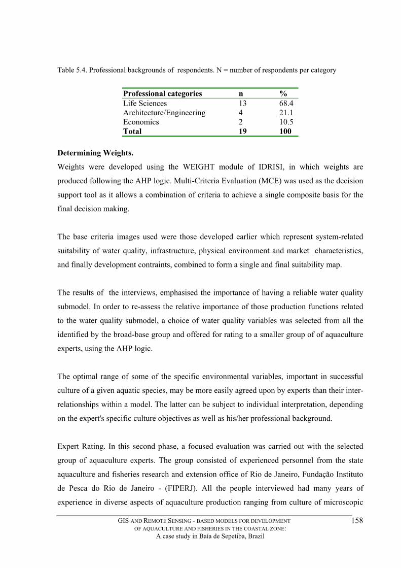
Table 5.4. Professional backgrounds of respondents. N = number of respondents per category

Determining Weights.

Weights were developed using the WEIGHT module of IDRISI, in which weights are

produced following the AHP logic. Multi-Criteria Evaluation (MCE) was used as the decision

support tool as it allows a combination of criteria to achieve a single composite basis for the

final decision making.

n

The base criteria images used were those developed earlier which represent system-related

suitability of water quality, infrastructure, physical environment and market characteristics,

and finally development contraints, combined to form a single and final suitability map.

Professional categories % 13 68.4

21.1 Economics 2 10.5 Total 19

Life Sciences Architecture/Engineering 4

100

The results of the interviews, emphasised the importance of having a reliable water quality

submodel. In order to re-assess the relative importance of those production functions related

to the water quality submodel, a choice of water quality variables was selected from all the

identified by the broad-base group and offered for rating to a smaller group of of aquaculture

experts, using the AHP logic.

The optimal range of some of the specific environmental variables, important in successful

culture of a given aquatic species, may be more easily agreed upon by experts than their inter-

relationships within a model. The latter can be subject to individual interpretation, depending

on the expert's specific culture objectives as well as his/her professional background.

Expert Rating. In this second phase, a focused evaluation was carried out with the selected

group of aquaculture experts. The group consisted of experienced personnel from the state

aquaculture and fisheries research and extension office of Rio de Janeiro, Fundação Instituto

de Pesca do Rio de Janeiro - (FIPERJ). All the people interviewed had many years of

experience in diverse aspects of aquaculture production ranging from culture of microscopic



158

algae, rotifers, marine shrimp, mussels and oysters. This second interview phase was carried

out on 12/8/98. The group was asked to rate the following aquaculture production variables:

Salinity, Dissolved Oxygen, Temperature, Chlorophyll-a and Faecal coliforms (Escherichia

coli count). Secondly the group was asked to rate Markets, Siting, Technical Support,

Fishermen Location and Seed Availability in an overall model. The experts were asked to use

the nine-point scale illustrated in Figure 5.1, where one variable must be rated in terms of its

importance relative to another.

Fig. 5.1. Pairwise 9 point pairwise comparison scale menu from Idrisi Weight module.

The aquaculture production functions were presented as a group in a ‘Water Quality Sub-

model’, which the experts were asked to rate by pairwise comparison, filling in a matrix of

cells, moving from column to column from left to right, generating a Pairwise Comparison

File (PCF). Each cell was considered relative in importance of the row variable to its

corresponding column variable as illustrated in Figure 5.2, using the nine-point scale. The

result of these interviews is summarised in Table 5.5.

Fig. 5.2. Example of rating with 9 point pairwise comparison scale using water quality criteria image files (Salinity, Dissolved Oxygen content, Water Temperature, Chlorophyll-a content, and Faecal coliforms (Escherichia coli count) in IDRISI.



159

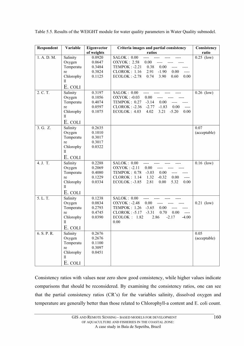
Table 5.5. Results of the WEIGHT module for water quality parameters in Water Quality submodel.

Respondent Criteria images and partial consistency ratios

Variable Eigenvector

of weights Consistency

ratio 1. A. D. M. Salinity

Oxygen Temperature Chlorophyll E. COLI

0.0647 0.3484 0.3824 0.1125

OXYOK : 2.58 0.00 ---- ---- ----

ECOLOK : -2.78 0.74 3.90 0.60 0.00

0.0920 SALOK : 0.00 ---- ---- ---- ----

TEMPOK : -2.21 0.38 0.00 ---- ---- CLOROK : 1.16 2.91 -1.90 0.00 ----

0.25 (low)

2. C. T. Salinity

CLOROK : -2.36 -2.77 -1.83 0.00 ----

Oxygen

E. COLI

0.3197 0.1056 0.4074 0.0597 0.1075

SALOK : 0.00 ---- ---- ---- ---- OXYOK : -0.03 0.00 ---- ---- ---- TEMPOK : 0.27 -3.14 0.00 ---- ----

ECOLOK : 4.03 4.02 3.21 -5.20 0.00

0.26 (low)

3. G. Z.

Temperature Chlorophyll

Salinity Oxygen Temperature Chlorophyll

0.2635

0.3017

0.07 (acceptable) 0.1010

0.3017

0.0322

E. COLI 4. J. T. Salinity

Oxygen

E. COLI

0.2069 0.4080

0.0334

SALOK : 0.00 ---- ---- ---- ----

TEMPOK : 0.78 -3.03 0.00 ---- ----

0.16 (low) 0.2288 OXYOK : -2.11 0.00 ---- ---- ----

Temperature Chlorophyll

0.1229 CLOROK : 1.14 1.32 -0.32 0.00 ---- ECOLOK : -3.85 2.81 0.00 5.32 0.00

5. L. T. Salinity Oxygen Temperature Chlorophyll

OXYOK : -2.48 0.00 ---- ---- ----

CLOROK : -5.17 -3.31 0.70 0.00 ----

0.21 (low) 0.1238

E. COLI

0.0834 0.2793 0.4745 0.0390

SALOK : 0.00 ---- ---- ---- ----

TEMPOK : 1.26 -3.65 0.00 ---- ----

ECOLOK : 1.82 2.86 -2.17 -4.00 0.00

6. S. P. R. Salinity Oxygen Temperature Chlorophyll E. COLI

0.2676 0.2676 0.1100 0.3097 0.0451

0.05 (acceptable)

Consistency ratios with values near zero show good consistency, while higher values indicate

comparisons that should be reconsidered. By examining the consistency ratios, one can see

that the partial consistency ratios (CR’s) for the variables salinity, dissolved oxygen and

temperature are generally better than those related to Chlorophyll-a content and E. coli count.



160

This may be because whereas, the former variables have a more direct relation to the

physiological requirements predominant in most marine organisms, the latter can be

interpreted in two ways: If high values are found, they may indicate good water quality

conditions, rich in algal content important for shellfish nutrition, or alternatively, as an

indication of water quality deterioration. In excessive amounts, such as noxious dinoflagelate

blooms they can be a hazard to human health. Only one third of the replies met acceptable

consistency ratios that would support use of the variable weights in MCE analysis.

During the same interview session, the aquaculture experts were asked to rate other

production related variables detected by the larger borad-based group as important, and so,

considered in this research as sub-models on their own.

The results are shown in Table 5.6. Markets, in terms of their existence, size and general

acceptance of fishery/aquaculture products; Site, as a general indication of the infrastructure

and accessibility to the road network, to services and goods important for production.

Technical Support, as in the availability of trained aquaculture experts to assist in all phases

of production; Fishermen location, as in their proximity to the natural conditions and

appropriate environment for aquaculture production purposes and finally Seed availability,

either as in the possibility of obtaining naturally occuring or laboratory produced starting

stock for production. It can be seen that 66.6% of the interviewed group achieved acceptable

CR’s in their pairwise comparisons between submodels. The participants who obtained low

consistency ratios in their pairwise comparisons had lowest CR’s for those factors pertaining

directly to their participation in the aquaculture process, i.e. Technical support (CR=3.77) or

Seed Availability ( as in lab produced seed) CR=5.86, which may indicate a bias in their

response.



161

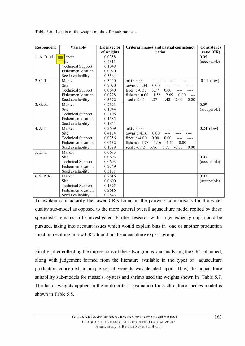
Table 5.6. Results of the weight module for sub models.

Respondent Variable Eigenvector of weights

Criteria images and partial consistency ratios

Consistency ratio (CR)

1. A. D. M. Market Site Technical Support Fishermen location 0.0920

(acceptable)

Seed availability

0.0358 0.4311 0.1048

0.3364

0.05

2. C. T. Market Site Technical Support Fishermen location

0.2070 0.0640 0.0278

towns : 1.34 0.00 ---- ---- ---- fiperj : -0.37 3.77 0.00 ---- ---- fishers : 0.00 1.55 2.69 0.00 ---

0.3440 mkt : 0.00 ---- ---- ---- ---- 0.11 (low)

Seed availability 0.3572 seed : 0.04 -1.27 -1.42 2.00 0.00 3. G. Z. Market 0.2621

0.09 (acceptable)

Site 0.1844

Technical Support 0.2106 0.1585 Fishermen location

Seed availability 0.1844 4. J. T.

Site Technical Support Fishermen location Seed availability

0.4174 0.0356

mkt : 0.00 ---- ---- ---- ----

fishers : -1.78 1.16 -1.51 0.00 ---

Market 0.3609

0.0532 0.1329

To explain satisfactorily the lower CR’s found in the pairwise comparisons for the water

quality sub-model as opposed to the more general overall aquaculture model replied by these

specialists, remains to be investigated. Further research with larger expert groups could be

pursued, taking into account issues which would explain bias in one or another production

function resulting in low CR’s found in the aquaculture experts group.

Finally, after collecting the impressions of these two groups, and analysing the CR’s obtained,

along with judgement formed from the literature available in the types of aquaculture

production concerned, a unique set of weights was decided upon. Thus, the aquaculture

suitability sub-models for mussels, oysters and shrimp used the weights shown in Table 5.7.

The factor weights applied in the multi-criteria evaluation for each culture species model is

shown in Table 5.8.

towns : 4.16 0.00 ---- ---- ---- fiperj : -4.00 0.00 0.00 ---- ----

seed : -3.72 5.86 0.73 -0.50 0.00

0.24 (low)

5. L. T. Market Site

Fishermen location 0.2749

Technical Support

Seed availability

0.0693 0.0693 0.0693

0.5171

0.03 (acceptable)

6. S. P. R. Market

Technical Support Fishermen location Seed availability

0.2616 0.0600

0.2616 0.2843

0.1325

Site

0.07 (acceptable)



162

Lindsay Ross

Depersonalise?

Table 5.7. Factor weights used in Multi-criteria evaluation mollusc suitability sub-models

Mollusc Mussel Oyster Submodel/filename Factor weights Factor weights

Water Quality

Table 5.8. Factor weights used in Multi-criteria evaluation mollusc suitability model

Submodel Factor weights Factor weights Oyster Mussel

Water Quality 0.3999 0.2860 Infrastructure 0.1076 0.1002

0.2653 0.1602 Market 0.2272 0.4536 Consistency Ratio 0.06 0.10

Physical Factors

Mcemuss Oystwq Temperature 0.4343 0.4399 Salinity 0.2079 0.2069 Dissolved Oxygen 0.2183 0.1950 Chlorophyll-a content

0.1119 0.1262

E. coli content 0.0276 0.0320 Consistency Ratio 0.06 0.06

Infrastructure Infra Oytinfra Technical assistance 0.0723 0.0983 Roads 0.0723 0.1586 Fishermen 0.4277 0.2270 Seed 0.4277 0.5161 Consistency Ratio 0.01 0.05

Physical Factors physmus Oytphys Wave exposure 0.6586 0.5396 Current velocity 0.1562 0.2970 Depth aproprpriate 0.1852 0.1634 Consistency Ratio 0.03 0.01

Markets Mkts Mkts Market distance 0.1562 0.1562 Buying Power 0.6586 0.6586 Fish Consumption 0.1852 0.1852 Consistency Ratio 0.03 0.03



163

Water temperature was considered the most important criterion of this submodel, followed

very closely by Salinity, Dissolved Oxygen, and Chlorophyll-a as an indication of food source

in the water (Table 5.9).

Fig. 5.3. Mollusc aquaculture site suitability model developed for Sepetiba Bay.

5.1.1 - Water quality sub-model

Mussels. The faecal coliform count in the water, although important from the point of view of

a potential human health hazard, was considered less important than the other factors in terms

of adequacy for mussel growth. Mussels are known to thrive in waters with significant

numbers of faecal coliforms, however they can become stressed if they are subjected to spend



164

many hours in waters with low dissolved oxygen levels, or salinity which is not within its

preferred range.

Table 5.9. Pairwise comparison matrix for mussel water quality submodel. Results of Multi-Criteria Evaluation for water quality sub-model. The eigenvector of the weights applied is: Temperature: 0.4343; Salinity: 0.2079; Dissolved oxygen: 0.2183; Chlorophyll: 0.1119; Faecal coliforms: 0.0276. The result is a 0.06 consistency ratio which is acceptable.

Factor

Temperature

Salinity

Dissolved oxygen

Chlorophyll

Faecal

coliforms Temperature 1 Salinity 1/3 1

1/3 1 1 Chlorophyll 1/3 1/3 1/3 Faecal coliforms 1/9 1/7 1/9 1/7 1

Dissolved oxygen 1

Oysters. The pairwise comparison matrix shown in Table 5.10 is very similar to the mussel

water quality sub-model, because both organisms share many environmental requirements.

However, slightly more importance was given to the faecal coliform count variable because

oysters are very often cultured closer to the shore and are therefore more exposed to sewage

runoff than cultured mussels. Oysters are also frequently eaten uncooked. Higher coliform

counts could be an indication of higher water temperatures and also more polluted water

conditions, while dissolved oxygen levels remain within the acceptable range. Chlorophyll-a

content was also considered slightly more important in the oyster sub-model than in the

mussel sub-model because oysters are more limited in their feeding requirements, requiring

specific sizes and qualities of phytoplankton for good growth.

Table 5.10. Pairwise comparison matrix for oyster water quality sub-model. Results of Multi-Criteria Evaluation for water quality sub-model. The eigenvector of the weights applied are: Temperature: 0. 4399; Salinity: 0.2069; Dissolved oxygen: 0.1950; Chlorophyll: 0.1262; Faecal coliforms: 0.0320. The result is a 0.06 consistency ratio, which is acceptable

Factor

Temperature

Salinity

Dissolved

oxygen

Chlorophyll

Faecal

coliforms Temperature 1 Salinity 1/3 1 Dissolved oxygen 1/3 1 1 Chlorophyll 1/3 1/3 1/2 1 Faecal coliforms 1/9 1/5 1/7 1/7 1



165

5.1.2 - Infrastructure

The infrastructure sub-model was based on distance maps of potential culture sites from

infrastructural elements. These are technical support (based in the region and represented by

personnel of the local fisheries research and extension office FIPERJ), the local roads

network, the fishing villages and/or community co-op centers from which culture operations

could be based, as well as distance from wild mussel banks ocurring in the bay, or oyster spat

obtained in natural spatfall in mangrove areas i.e. primary seed sources. Mussel seed are

found on rocks and rocky shores of islands in the bay, and were digitised on screen following

site verificatioin during field trips. Oyster spatfall area was considered equal to all mangrove

areas. The rationale for deriving weights in this sub-model attributed relatively more

importance to the actual distance from the fishermen's home base as well as from mussel seed

sources, as it is thought that these two elements are more critical for production. Although

technical support is also deemed important, it is probably only as important as access to roads

when mussel farmers need to find support and solutions to technical problems, but much less

important than distance from culture site for day-to-day management and culture ‘starter’

seed.

.

Mussels. Technical support, in the form of visits from fisheries extension agents depends on

the difficulty of access to the potential sites. The local fisheries extension service, has a

roadside base, so, any site close to a road, is relatively easily accessible. However, reaching

those fishermen sites which may be on islands, or in mangrove areas, accessible only by boat,

imposes greater difficulty hence the 'strongly more important' rating given in the PCF shown

in Table 5.11.

During the course of this research, many of the fishermen residential sites were visited and it

was seen that very few were close to roads. Another most important factor is the distance

from sites where mussel seed naturally occur. This was found to be more important than

distance to technical support, as many a fisherman has started his own mussel culture

wherever seed supply is available, even if he may have little or no technical support. By the

same token, it is accepted that communication among fishermen is important in transmitting

information and cultural practices, such as aquaculture. Thus, closeness to naturally occurring

mussel seed banks was less important than distance to other fishermen or fishemen

organization such as a coop.



166

Lindsay Ross

Could spatfall not occur beyond the mangroves? – currents etc will spread the larvae and they will settle elsewhere if the substrate is OK.

Table 5.11. Pairwise comparison matrix for mussel infrastructure sub-model. Results of Multi-Criteria Evaluation for infrastructure sub-model. The eigenvector of the weights thus applied is: Technical support 0.0723 Distance from roads 0.0723; Distance from fishermen villages/coops: 0.4277; Distance from mussel seed sites: 0.4277. The result is a 0.01 consistency ratio, which is acceptable.

Factor

Technical support

Distance

from roads

Distance from

fishermen villages/

coops

Distance from

mussel seed sites

Technical support Distance from roads 1 1 Distance from fishermen villages/ coops 7 5 1 Distance from mussel seed sites 5 7 1/3 1

1

Oysters. Considering that the native oyster C. rhizophorae is most likely to be farmed closer

to the mainland shores, instead of on island fringes, slightly less importance was given to

distance from technical support than in the mussel pairwise comparison matrix, because these

sites would be more easily accessible by vehicle/boat combination (Table 5.12), and also,

because fishermen coops on the continent are on the roadside. However, distance from an

oyster seed production facility, such as the local fisheries lab, or mangrove spat settling sites,

was considered strongly more important than technical support, because, there is only one

oyster producing lab in the state, and because collection of natural oyster spatfall in

mangroves is still not practised in the region. If fishermen have easy access by means of their

own canoes, or reasonable walking distance to the fisheries lab, or mangrove areas where they

can collect oyster spat, distance to the road network becomes less important.

Likewise, closeness can facilitate exchanges and bartering including oyster seed for starting

their own culture.

Table 5.12. Pairwise comparison matrix for oyster infrastructure sub-model. Results of Multi-Criteria Evaluation for infrastructure sub-model. The eigenvector of the weights thus applied is: Technical support 0.0983 Distance from roads 0.1586; Distance from fishermen villages/coops: 0.2270; Distance from mussel seed sites: 0.5161. The result is a 0.05 consistency ratio, which is acceptable.



167

Factor

Technical support

Distance

from roads

Distance from

fishermen villages/

coops

Distance

from mussel

seed sites Technical support 1 Distance from roads 1 1 Distance from fishermen villages/ coops 3 1 1 Distance from oyster banks in mangroves or fisheries lab.

7 3 2 1

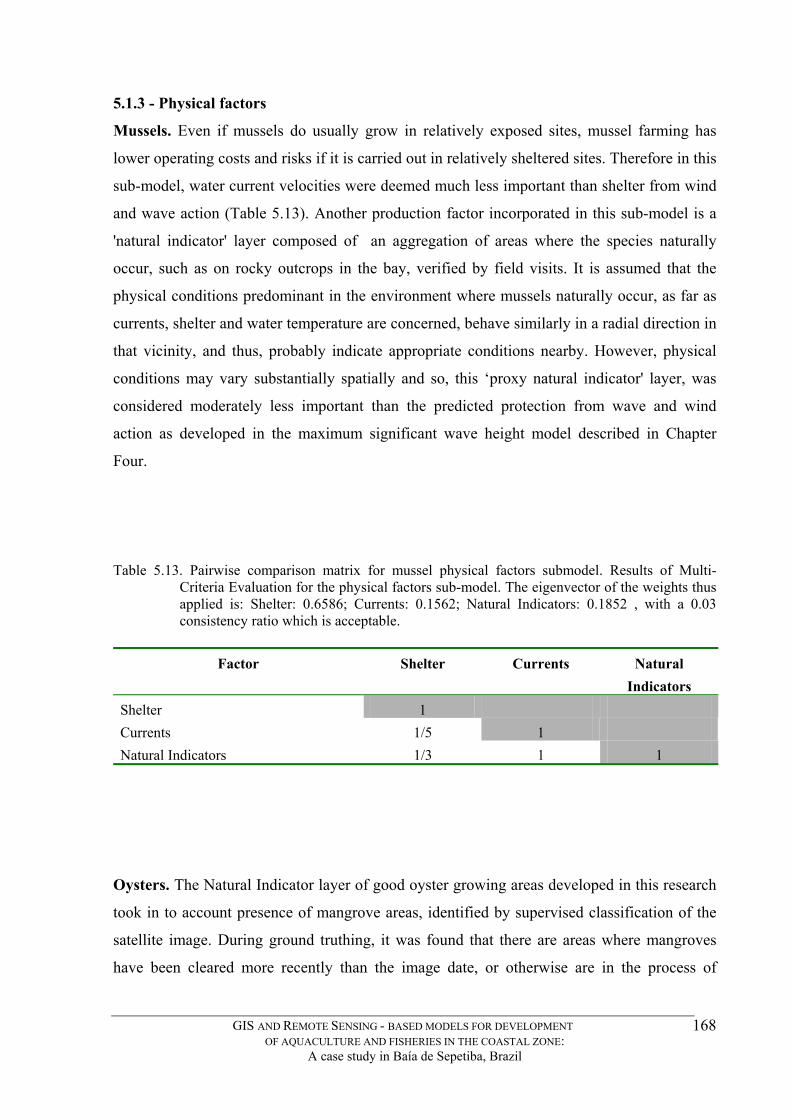
5.1.3 - Physical factors

Mussels. Even if mussels do usually grow in relatively exposed sites, mussel farming has

lower operating costs and risks if it is carried out in relatively sheltered sites. Therefore in this

sub-model, water current velocities were deemed much less important than shelter from wind

and wave action (Table 5.13). Another production factor incorporated in this sub-model is a

'natural indicator' layer composed of an aggregation of areas where the species naturally

occur, such as on rocky outcrops in the bay, verified by field visits. It is assumed that the

physical conditions predominant in the environment where mussels naturally occur, as far as

currents, shelter and water temperature are concerned, behave similarly in a radial direction in

that vicinity, and thus, probably indicate appropriate conditions nearby. However, physical

conditions may vary substantially spatially and so, this ‘proxy natural indicator' layer, was

considered moderately less important than the predicted protection from wave and wind

action as developed in the maximum significant wave height model described in Chapter

Four.

Table 5.13. Pairwise comparison matrix for mussel physical factors submodel. Results of Multi-Criteria Evaluation for the physical factors sub-model. The eigenvector of the weights thus applied is: Shelter: 0.6586; Currents: 0.1562; Natural Indicators: 0.1852 , with a 0.03 consistency ratio which is acceptable.

Factor Shelter Currents Natural

Indicators Shelter 1 Currents 1/5 1

1/3 1 1 Natural Indicators

Oysters. The Natural Indicator layer of good oyster growing areas developed in this research

took in to account presence of mangrove areas, identified by supervised classification of the

satellite image. During ground truthing, it was found that there are areas where mangroves

have been cleared more recently than the image date, or otherwise are in the process of



168

regeneration after clearance. In this way, this layer may not be totally adequate to indicate all

areas otherwise suitable for oyster growth. Considering that oysters generally tend to be

cultured in the shallows of estuaries and protected areas of bays, current velocities were

considered slightly less important than in the oyster factors PCF (Table 5.14). Natural

indicators of oyster areas, were considered slightly less important than local current velocities,

which may vary significantly in branches of mangrove estuaries and shallow areas.

Table 5.14. Pairwise comparison matrix for oyster physical factors sub-model. Results of Multi-Criteria Evaluation for the physical factors sub-model. The eigenvector of the weights thus applied is: Shelter: 0.5396; Currents: 0.2970; Natural Indicators: 0.1634 , with a 0.015 consistency ratio, which is acceptable.

Factor Shelter Currents Natural Indicators

Shelter 1 Currents 1/2 Natural Indicators 1/3 1/2 1

1

5.1.4 - Markets

A single pairwise comparison matrix was developed for all the species sub-models, as, in

general, seafoods can be grouped together as opposed to other animal protein sources such as

cattle, pig, chicken meat, the most commonly available alternatives in the area. Mimimum

wages (MW) per household income was taken as an indication of consumer buying power for

seafood acquisition.

This factor was considered more important than actual fish consumption per capita, or fish

consumtion habit or distance to fish markets (Table 5.15). If consumers do not have the

money to pay seafood producers for their aquaculture production, it is hardly feasible for the

latter to engage profitably in the activity. However, if consumers have more available income

to spend on seafood including ‘value added’ products, then marketing strategies could be

developed to encourage higher seafood consumption. While market distances to the producing

areas remain relatively the same over time or even, relatively speaking, can diminish as roads

improve and urban areas expand, household income can vary more significantly, limiting or

expanding demand. In the context of Brazil, it should be noted that seafood consumption habit

is much lower than red or white meat consumption, a cultural characteristic. Currently,

educational campaigns and public awareness of the advantages to health in consuming

seafood suggest an increase in demand. However, in this sub-model, seafood consumption



169

habit was considered less important than actual distance to market, and much less important

than consumer buying power.

Table 5.15. Pairwise comparison matrix for the markets submodel Results of the Markets sub-model. The eigenvector of the weights thus applied are: Market distance: 0.2883; Consumer buying power: 0.6370; Fish consumption habit: 0.1047, with a 0.015 consistency ratio, which is acceptable. Factor Market distance Consumer buying

power Fish consumption

habits Market distance 1 Consumer buying power 3 Fish consumption habit 1/3 1/5 1

1

Mollusc models final MCE . Tables 5.16 and 5.17 summarise the relative importance of the

sub-models in the context of mussel and oyster culture development potential.

Table 5.16. Pairwise comparison matrix for the Mussel model. Results of Multi-Criteria Evaluation for the mussel model. The eigenvector of the weights thus applied are: Water Quality: 0.2860; Infrastructure: 0.1002; Physical Factors: 0.1602 and Markets 0.4536., with a 0.1 consistency ratio which is acceptable.

Factor MCE- Water Quality

MCE- Infrasturcuture

MCE- Physical Factors

MCE- Markets

MCE-Water Quality 1 MCE- Infrasturcuture 1/3 1 MCE- Physical Factors 1/3 2 1 MCE- Markets 3 3 2 1

Table 5.17. Pairwise comparison matrix for the Oyster model. Results of the Multi-Criteria Evaluation for the oyster model. The eigenvector of the weights thus applied are: Water Quality: 0.3999; Infrastructure: 0.1076; Physical Factors: 0.2653 and Markets 0.2272., with a 0.06 consistency ratio which is acceptable.

Factor MCE- Water Quality

MCE- Infrastrucuture


MCE- Markets

MCE-Water Quality 1 MCE- Infrasturcuture 1/3 1 MCE- Physical Factors 1 2 1 MCE- Markets 1/3 3 2 1



170

5.1.5 - Shrimp Farming Site Selection Model

The shrimp farming site selection model is designed as illustrated in Figure 5.4. It follows a

rationale and design similar to that developed for mollusc farming site selection, discussed

previously. Two main differences are the absence of a water quality sub-model and emphasis

given on a climatic a natural indicator sub-model. This is explained by the fact that shrimp

farming activity is carried out over land and not over seawater, and so, it is affected more

directly by climatic factors such as air temperature, rainfall, and soil quality, which are not so

relevant in open waters because of the importance of seawater circulation. Although

technically, any area along the coastline could be a source for abstraction of seawater for

shrimp pond filling. Because of the hilly topography of islands in the the bay, only the

continental lands and the larger Marambaia island were considered in the modelling. Other

peculiarities are discussed in each sub-model. The pairwise comparison matrices for each sub-

model were arrived at by reviewing the expert panels questionnaire results and by arriving at a

consensus based on discussions held with a collaborating shrimp farming expert.



171

Fig. 5.4. Shrimp farming site suitability model development for Sepetiba 5.1.5.1 - Infrastructure sub-model

The shrimp farming potential infrastructure sub-model followed a, similar rationale to that

employed in the mussel and oyster models, i.e. it was based on distance of potential culture

sites in the continental area of Sepetiba Bay region to several infrastructural elements.



172

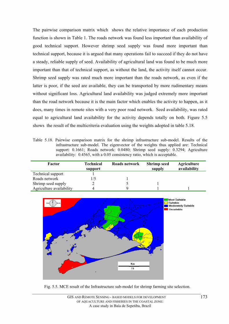
The pairwise comparison matrix which shows the relative importance of each production

function is shown in Table 1. The roads network was found less important than availability of

good technical support. However shrimp seed supply was found more important than

technical support, because it is argued that many operations fail to succeed if they do not have

a steady, reliable supply of seed. Availability of agricultural land was found to be much more

important than that of technical support, as without the land, the activity itself cannot occur.

Shrimp seed supply was rated much more important than the roads network, as even if the

latter is poor, if the seed are available, they can be transported by more rudimentary means

without significant loss. Agricultural land availability was judged extremely more important

than the road network because it is the main factor which enables the activity to happen, as it

does, many times in remote sites with a very poor road network. Seed availability, was rated

equal to agricultural land availability for the activity depends totally on both. Figure 5.5

shows the result of the multicriteria evaluation using the weights adopted in table 5.18.

Table 5.18. Pairwise comparison matrix for the shrimp infrastructure sub-model. Results of the infrastructure sub-model. The eigenvector of the weights thus applied are: Technical support: 0.1661; Roads network: 0.0480; Shrimp seed supply: 0.3294; Agriculture availability: 0.4565, with a 0.05 consistency ratio, which is acceptable.

Factor Technical support

Roads network Shrimp seed supply

Agriculture availability

Technical support 1 Roads network 1/5 1 Shrimp seed supply 2 5 1 Agriculture availability 4 9 1 1

Fig. 5.5. MCE result of the Infrastructure sub-model for shrimp farming site selection.



173

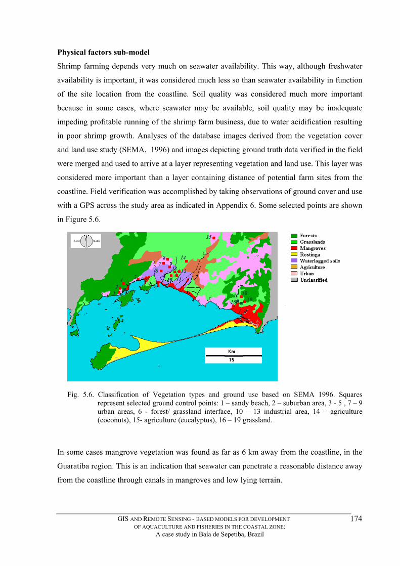
Physical factors sub-model

Shrimp farming depends very much on seawater availability. This way, although freshwater

availability is important, it was considered much less so than seawater availability in function

of the site location from the coastline. Soil quality was considered much more important

because in some cases, where seawater may be available, soil quality may be inadequate

impeding profitable running of the shrimp farm business, due to water acidification resulting

in poor shrimp growth. Analyses of the database images derived from the vegetation cover

and land use study (SEMA, 1996) and images depicting ground truth data verified in the field

were merged and used to arrive at a layer representing vegetation and land use. This layer was

considered more important than a layer containing distance of potential farm sites from the

coastline. Field verification was accomplished by taking observations of ground cover and use

with a GPS across the study area as indicated in Appendix 6. Some selected points are shown

in Figure 5.6.

Fig. 5.6. Classification of Vegetation types and ground use based on SEMA 1996. Squares represent selected ground control points: 1 – sandy beach, 2 – suburban area, 3 - 5 , 7 – 9 urban areas, 6 - forest/ grassland interface, 10 – 13 industrial area, 14 – agriculture (coconuts), 15- agriculture (eucalyptus), 16 – 19 grassland.

In some cases mangrove vegetation was found as far as 6 km away from the coastline, in the

Guaratiba region. This is an indication that seawater can penetrate a reasonable distance away

from the coastline through canals in mangroves and low lying terrain.



174

Soil quality was considered to be much more important than freshwater sources, because,

sandy soils and cambissols present in the study area, would make for very poor ponds because

of high seepage rates adding to costs in the business. Replenishing ponds with available

freshwater sources would not solve the problem. Due to the indications that natural vegetation

gives us as to the quality of the environment, this vegetation and ground cover layer was

considered much more important than closeness to a freshwater source. However vegetation

and land use was considered slightly less important than soil quality, mostly because soil

quality changes less significantly than vegetation cover and land use. The pairwise

comparison matrix which shows the relative importance of each production function is shown

in Table 5.19. Figure 5.7 shows the result of multicriteria evaluation using the weights

adopted in table 5.19.

Table 5.19 Pairwise comparison matrix for the shrimp Physical Factors sub-model.. Results of the Physical Factors sub-model. The eigenvector of the weights thus applied are: Marine Coastline: 0.1275; Freshwater Sources: 0.0569; Soil Quality: 0.5590; Vegetation and Land Use: 0.2566 with a 0.04 consistency ratio, which is acceptable.

Marine Coastline

Factor Freshwater Sources

Soil Quality Vegetation and Land Use

Marine Coastline 1 Freshwater Sources 1/3

4 3 1

1 Soil Quality 8 1 Vegetation and Land Use 4 1/3

Fig. 5.7. MCE result of the Physical Factors sub-model for shrimp farming site selection.



175

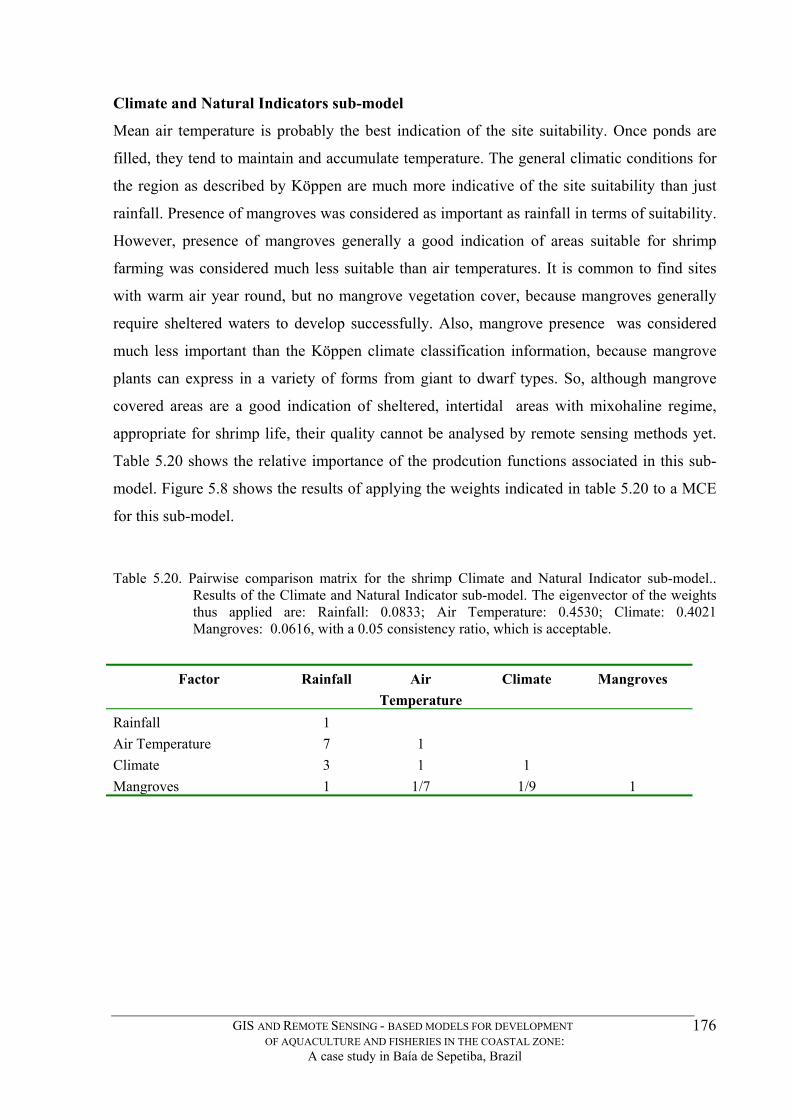
Climate and Natural Indicators sub-model

Mean air temperature is probably the best indication of the site suitability. Once ponds are

filled, they tend to maintain and accumulate temperature. The general climatic conditions for

the region as described by Köppen are much more indicative of the site suitability than just

rainfall. Presence of mangroves was considered as important as rainfall in terms of suitability.

However, presence of mangroves generally a good indication of areas suitable for shrimp

farming was considered much less suitable than air temperatures. It is common to find sites

with warm air year round, but no mangrove vegetation cover, because mangroves generally

require sheltered waters to develop successfully. Also, mangrove presence was considered

much less important than the Köppen climate classification information, because mangrove

plants can express in a variety of forms from giant to dwarf types. So, although mangrove

covered areas are a good indication of sheltered, intertidal areas with mixohaline regime,

appropriate for shrimp life, their quality cannot be analysed by remote sensing methods yet.

Table 5.20 shows the relative importance of the prodcution functions associated in this sub-

model. Figure 5.8 shows the results of applying the weights indicated in table 5.20 to a MCE

for this sub-model.

Table 5.20. Pairwise comparison matrix for the shrimp Climate and Natural Indicator sub-model.. Results of the Climate and Natural Indicator sub-model. The eigenvector of the weights thus applied are: Rainfall: 0.0833; Air Temperature: 0.4530; Climate: 0.4021 Mangroves: 0.0616, with a 0.05 consistency ratio, which is acceptable.

Factor Rainfall Air Temperature

Climate Mangroves

7 1

Climate 3 1 1 Mangroves 1 1/7 1

Rainfall 1 Air Temperature

1/9



176

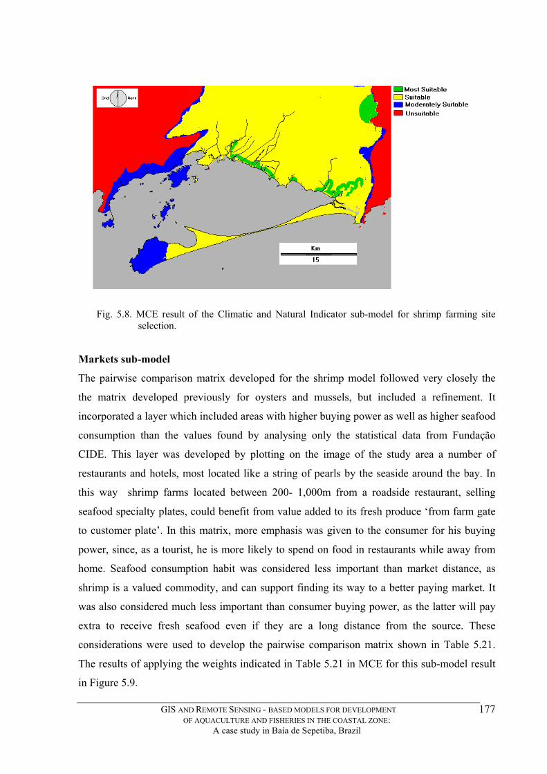
Fig. 5.8. MCE result of the Climatic and Natural Indicator sub-model for shrimp farming site

selection. Markets sub-model

The pairwise comparison matrix developed for the shrimp model followed very closely the

the matrix developed previously for oysters and mussels, but included a refinement. It

incorporated a layer which included areas with higher buying power as well as higher seafood

consumption than the values found by analysing only the statistical data from Fundação

CIDE. This layer was developed by plotting on the image of the study area a number of

restaurants and hotels, most located like a string of pearls by the seaside around the bay. In

this way shrimp farms located between 200- 1,000m from a roadside restaurant, selling

seafood specialty plates, could benefit from value added to its fresh produce ‘from farm gate

to customer plate’. In this matrix, more emphasis was given to the consumer for his buying

power, since, as a tourist, he is more likely to spend on food in restaurants while away from

home. Seafood consumption habit was considered less important than market distance, as

shrimp is a valued commodity, and can support finding its way to a better paying market. It

was also considered much less important than consumer buying power, as the latter will pay

extra to receive fresh seafood even if they are a long distance from the source. These

considerations were used to develop the pairwise comparison matrix shown in Table 5.21.

The results of applying the weights indicated in Table 5.21 in MCE for this sub-model result

in Figure 5.9.



177

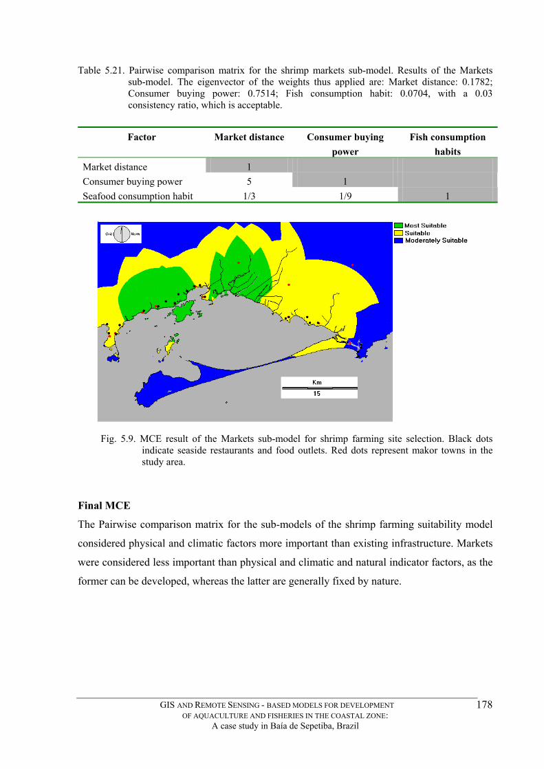
Table 5.21. Pairwise comparison matrix for the shrimp markets sub-model. Results of the Markets sub-model. The eigenvector of the weights thus applied are: Market distance: 0.1782; Consumer buying power: 0.7514; Fish consumption habit: 0.0704, with a 0.03 consistency ratio, which is acceptable.

Factor Market distance Consumer buying power

Fish consumption habits

Market distance 1 Consumer buying power 5 1 Seafood consumption habit 1/3 1/9 1

Fig. 5.9. MCE result of the Markets sub-model for shrimp farming site selection. Black dots indicate seaside restaurants and food outlets. Red dots represent makor towns in the study area.

Final MCE

The Pairwise comparison matrix for the sub-models of the shrimp farming suitability model

considered physical and climatic factors more important than existing infrastructure. Markets

were considered less important than physical and climatic and natural indicator factors, as the

former can be developed, whereas the latter are generally fixed by nature.



178

Table 5.22. Pairwise comparison matrix for the Shrimp model. Results of Multi-Criteria Evaluation for the shrimp model. The eigenvector of the weights thus applied are: Infrastructure: 0.1250; Physical Factors: 0.3750 Climate and Natural Indicators 0.3750 and Markets 0.1250., with a 0.00 consistency ratio which is acceptable.

Factor MCE- Infrastructure


MCE – Climate &

Natural Indicators

MCE- Markets

MCE- Infrastructure 1 MCE- Physical Factors 3 1 MCE – Climate 3 1 1 MCE- Markets 1 1/3 1/3 1

Fig. 5.10. Shrimp model site suitability according to multi-criteria evaluation. 5.2 - Results

5.2.1 - Mussel production potential

All the constraints and production factors for the mussel farming potential model were

processed in a final MCE. This result was further processed with FILTER to remove small

isolated groups and subsequently OVERLAYed with a DISTANCE generated buffer image

as described in Table 5.23. The purpose of this last overlay was to substantially narrow down

the potential areas within an even tighter spatial limit. The final result (Fig. 5.11) shows

three regions, or island groups with continuous areas of significant production potential:

Group 1 includes Ilha de Itacuruçá, closest to the continent. Group 2, embraces Ilha de

Jaguanum, located midway between the continent and I. da Marambaia, and Group 3, Ilha

Guaíba on the western end of the bay.



179

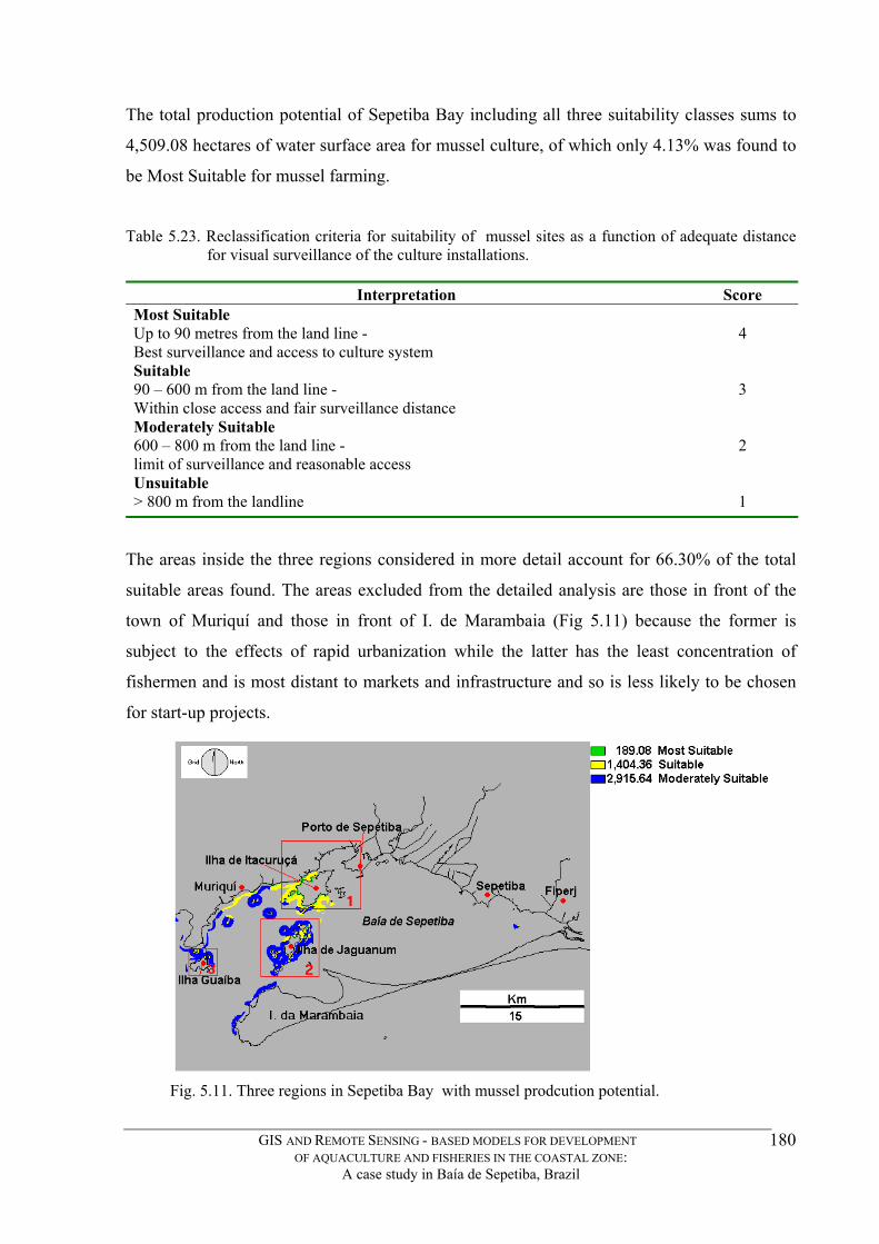
The total production potential of Sepetiba Bay including all three suitability classes sums to

4,509.08 hectares of water surface area for mussel culture, of which only 4.13% was found to

be Most Suitable for mussel farming.

Table 5.23. Reclassification criteria for suitability of mussel sites as a function of adequate distance for visual surveillance of the culture installations.


Most Suitable Up to 90 metres from the land line - Best surveillance and access to culture system

4

Suitable 90 – 600 m from the land line - Within close access and fair surveillance distance

3

Moderately Suitable 600 – 800 m from the land line - limit of surveillance and reasonable access

2

Unsuitable > 800 m from the landline

1

The areas inside the three regions considered in more detail account for 66.30% of the total

suitable areas found. The areas excluded from the detailed analysis are those in front of the

town of Muriquí and those in front of I. de Marambaia (Fig 5.11) because the former is

subject to the effects of rapid urbanization while the latter has the least concentration of

fishermen and is most distant to markets and infrastructure and so is less likely to be chosen

for start-up projects.

Fig. 5.11. Three regions in Sepetiba Bay with mussel prodcution potential.



180

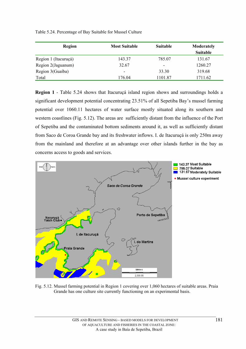
Table 5.24. Percentage of Bay Suitable for Mussel Culture

Region Most Suitable Suitable Moderately Suitable

Region 1 (Itacuruçá) 143.37 785.07 131.67 Region 2(Jaguanum) 32.67 - Region 3(Guaíba) - Total

1260.27 33.30 319.68

176.04 1101.87 1711.62

Region 1 - Table 5.24 shows that Itacuruçá island region shows and surroundings holds a

significant development potential concentrating 23.51% of all Sepetiba Bay’s mussel farming

potential over 1060.11 hectares of water surface mostly situated along its southern and

western coastlines (Fig. 5.12). The areas are sufficiently distant from the influence of the Port

of Sepetiba and the contaminated bottom sediments around it, as well as sufficiently distant

from Saco de Coroa Grande bay and its freshwater inflows. I. de Itacuruçá is only 250m away

from the mainland and therefore at an advantage over other islands further in the bay as

concerns access to goods and services.

Fig. 5.12. Mussel farming potential in Region 1 covering over 1,060 hectares of suitable areas. Praia

Grande has one culture site currently functioning on an experimental basis.



181

Recently (February, 2002) one of the sites predicted in this model (Praia Grande), was elected

by Universidade Castelo Branco as their site for implementing an experimental mussel

growing module.

No results are yet available, but the site was carefully chosen by a mollusc farming expert

with international experience. The adjacent mainland town of Itacuruçá certainly has enough

market potential for farmed mussel placement as it has a busy Yatch Club, is the main tourist

port for the ‘Costa Verde’ as the region is known, and includes several seaside restaurants. It

is also located very close to the main road network leading to larger markets in Rio and other

large towns.

Region 2 - Table 5.24 also shows that the Jaguanum island with its several peripheral smaller

islands has good mussel farm development as illustrated in Figure 5.13. A total of 1,578

hectares of suitable sites for mussel culture are found. This region accounts for 35% of all the

suitable areas for mussel culture found in Sepetiba Bay. It's potential success is enhanced by

the fact that it has a well established resident artisanal fishing community, a few small hotels

and is a “must” stop for schooners departing Itacuruçá port with tourists on 'Costa Verde'

tours for lunch and sunbathing.

Two potential sites in this region may generate area usage conflict. Nearby Ilha Bonita which

is mostly a resort island, and the southern side of Ilha Furtada which is a 'hot spot' for sport

fishing. Other good areas identified included as Suitable include Vigia Grande and Bernardo

islands, which are clearly good mussel growing areas as they have natural mussel banks

which were identified during field verification trips.



182

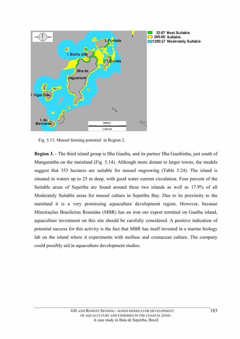
Fig. 5.13. Mussel farming potential in Region 2.

Region 3. - The third island group is Ilha Guaíba, and its partner Ilha Guaibinha, just south of

Mangaratiba on the mainland (Fig. 5.14). Although more distant to larger towns, the models

suggest that 353 hectares are suitable for mussel ongrowing (Table 5.24). The island is

situated in waters up to 25 m deep, with good water current circulation. Four percent of the

Suitable areas of Sepetiba are found around these two islands as well as 17.9% of all

Moderately Suitable areas for mussel culture in Sepetiba Bay. Due to its proximity to the

mainland it is a very promissing aquaculture development region. However, because

Mineirações Brasileiras Reunidas (MBR) has an iron ore export terminal on Guaíba island,

aquaculture investment on this site should be carefully considered. A positive indication of

potential success for this activity is the fact that MBR has itself invested in a marine biology

lab on the island where it experiments with mollusc and crustacean culture. The company

could possibly aid in aquaculture development studies.



183

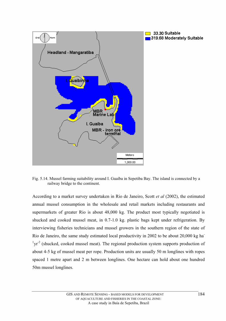
Fig. 5.14. Mussel farming suitability around I. Guaíba in Sepetiba Bay. The island is connected by a railway bridge to the continent.

According to a market survey undertaken in Rio de Janeiro, Scott et al (2002), the estimated

annual mussel consumption in the wholesale and retail markets including restaurants and

supermarkets of greater Rio is about 48,000 kg. The product most typically negotiated is

shucked and cooked mussel meat, in 0.7-1.0 kg. plastic bags kept under refrigeration. By

interviewing fisheries technicians and mussel growers in the southern region of the state of

Rio de Janeiro, the same study estimated local productivity in 2002 to be about 20,000 kg ha-

1yr-2 (shucked, cooked mussel meat). The regional production system supports production of

about 4-5 kg of mussel meat per rope. Production units are usually 50 m longlines with ropes

spaced 1 metre apart and 2 m between longlines. One hectare can hold about one hundred

50m mussel longlines.



184

This research identified 189 hectares of potential mussel cultivation areas classified as Most

Suitable in the three regions considered. in Sepetiba Bay. Based on the production figures

available for the region, a development of only 1.27 % (2.4 ha) of those areas considered as

best (Most Suitable) would suffice to satisfy the current demand for mussel meat in Rio de

Janeiro.

The metropolitan area markets could significantly increase current level of mussel demand by

promoting farmed-raised mussel production as a value-added product, i.e. with source and

quality guaranteed by appropriate health certification authority. As shown by the survey

carried out by Scott et al (2002), much of the mussel meat currently sold in the market is

harvested artisanally from sites along Guanabara Bay where it is cooked, shucked and bagged

by the seashore and sold in street markets and restaurants without any sanitary inspection or

health certification. It is reasonable to conclude that current demand can probably expand

considerably with a aquaculture quality product such as mussels farmed in Sepetiba.

Table 5.25. Summary of development needs and mussel farming potential for Sepebita bay.

Estimated mussel meat consumption/yr (Rio, metropolitan area ) 48,000 kg/yr

Estimated productivity of mussel (meat) 20,000 kg/ha/yr

Area of identified production sites classified as Most Suitable (hectares) 189.08ha

Production area needed do satisfy current demand (hectares) 2.4 ha

Percentage of total available Most Suitable areas necessary to satisfy Rio metropolitan mussel demand.

1.27%

* based on figures obtained from Ilha Grande mussel producers.

5.2.2 - Oyster culture potential

As shown in Fig. 5.15 the results of the oyster aquaculture potential model indicate three

distinct regions in the bay with good oyster farming potential. Region 1 is characterised by its

closeness to the mangroves in Guaratiba. Region 2 is the coastal zone between Itacuruçá and

Mangaratiba, and Region 3 is more isolated, on Marambaia Island.



185

Fig. 5.15. Three regions with significant potential for mangrove oyster cultivation.

Fig. 5.16 Oyster potential farming areas in the Guaratiba region. Mangroves indicated in green hatch Region 1. Figure 5.16 shows a close up on Region 1 where over 100 hectares of area

classified as Most Suitable areas for oyster culture exist. The main reasons for this are a)

environmental suitability and proximity to mangroves which are natural sites for oyster

growth, b) closeness to technical support base (FIPERJ lab) which is capable of producing

oyster seed, c) proximity to markets, general infrastructure, fishing communities, and d)

adequate distance from potential culture sites for sufficient surveillance, as re-classified and

indicated in Table 5.26.

Table 5.26. Reclassification criteria for suitability of oyster farming sites.

Interpretation Score Most Suitable Up to 300 metres from the coastline - Best surveillance and access to culture system

4

Suitable 300 - 460 m from the coastline - Within close access and fair surveillance distance

3

Moderately Suitable 460 - 570 m from the coastline - limit of surveillance and reasonable access

2 Unsuitable > 570 m from the coastline

1



186

Fig. 5.16. Region 1. Oyster potential farming areas, in the Guaratiba region surrounded by mangroves ( green hatch ). Region 2. This area is mostly contained along the coastal interstate highway BR-101 (Rio-

Santos) between the towns of Itacuruçá and Mangaratiba (Fig. 5.17). Several areas classified

as Most Suitable lie within close proximity of Itacuruçá, Muriquí and Praia Grande, coastal

towns with significant weekend tourist traffic. One experimental oyster culture operation in

fact exists on the island of Itacuruçá, very close to areas classified as most suitable.

Fig. 5.17. Region 2. Oyster potential farming areas, in the Itacuruçá - Mangaratiba region.



187

Region 3. In the Ilha de Marambaia zone, areas which are Suitable and Moderately Suitable

for oyster culture development cover 247 ha (Fig. 5.18). Although Ilha de Marambaia has

suitable areas it has only one small fishing community. Also in the same region, Ilha de

Jaguanum, although having a larger fishing settlement, and having natural oyster populations

growing on its rocky coastline, is somewhat constrained mostly because of the depth

constraint layer. The 0-3m depth area is very narrow. Potentially a system other than bottom

resting oyster racks could be employed in this area. In terms of its distance to markets on the

continent, to seed sources as well as physical factors including salinity, Ilha da Marambaia is

probably the site where oyster culture development would be first started. Because of its

position, Marambaia has a range potential zone. Figure 5.18 shows a range of Chlorophyll a

content as a backdrop in the predicted oyster production potential area. This observation may

be used in a subsequent opportunity to predict different growth rates.

Fig. 5.18. Region 2. Oyster potential farming areas, in the Marambaia region.



188

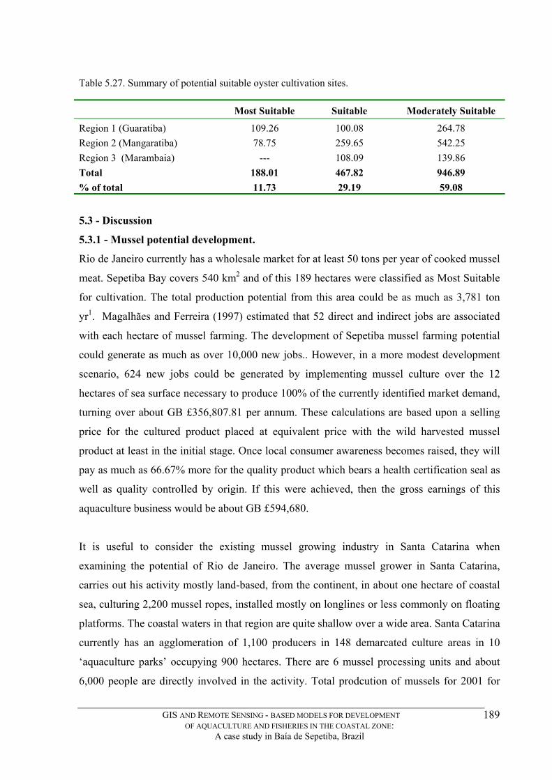
Table 5.27. Summary of potential suitable oyster cultivation sites. Moderately Suitable Most Suitable Suitable

Region 1 (Guaratiba) 109.26 100.08 264.78 Region 2 (Mangaratiba) 78.75 259.65 542.25 Region 3 (Marambaia) --- 108.09 139.86 Total 188.01 467.82 946.89 % of total 11.73 29.19 59.08

5.3 - Discussion

5.3.1 - Mussel potential development.

Rio de Janeiro currently has a wholesale market for at least 50 tons per year of cooked mussel

meat. Sepetiba Bay covers 540 km2 and of this 189 hectares were classified as Most Suitable

for cultivation. The total production potential from this area could be as much as 3,781 ton

yr1. Magalhães and Ferreira (1997) estimated that 52 direct and indirect jobs are associated

with each hectare of mussel farming. The development of Sepetiba mussel farming potential

could generate as much as over 10,000 new jobs.. However, in a more modest development

scenario, 624 new jobs could be generated by implementing mussel culture over the 12

hectares of sea surface necessary to produce 100% of the currently identified market demand,

turning over about GB £356,807.81 per annum. These calculations are based upon a selling

price for the cultured product placed at equivalent price with the wild harvested mussel

product at least in the initial stage. Once local consumer awareness becomes raised, they will

pay as much as 66.67% more for the quality product which bears a health certification seal as

well as quality controlled by origin. If this were achieved, then the gross earnings of this

aquaculture business would be about GB £594,680.

It is useful to consider the existing mussel growing industry in Santa Catarina when

examining the potential of Rio de Janeiro. The average mussel grower in Santa Catarina,

carries out his activity mostly land-based, from the continent, in about one hectare of coastal

sea, culturing 2,200 mussel ropes, installed mostly on longlines or less commonly on floating

platforms. The coastal waters in that region are quite shallow over a wide area. Santa Catarina

currently has an agglomeration of 1,100 producers in 148 demarcated culture areas in 10

‘aquaculture parks’ occupying 900 hectares. There are 6 mussel processing units and about

6,000 people are directly involved in the activity. Total prodcution of mussels for 2001 for



189

Santa Catarina was 11.364.85t in the year 2000, with a slight decrease for 2001 with 10,

667.10t. The shellfish growers in that state have a strong fisheries extension service

(EPAGRI) to support them, and a strong tourist business base.

In contrast, mussel growing in Rio de Janeiro has developed in a scattered fashion as rings

around islands such as Ilha Grande, separated from the continent by deeper waters (>7m).

Growers use exclusively the longline system where 2 - 12 longlines are spaced 2m apart, and

manage at most 600 mussel ropes.

The infrastructure of the sites where the current mussel growers are based (Ilha Grande), is

very poor, most not have electricity and must travel by boat to the continent for supplies and

services. According to Proença (2001) the region concentrates 89% of Rio de Janeiro state

mussel growers, which are estimated to be about 50, while another 30 sites are in the process

of development. Local statistics on fisheries is very poor, and there are only five extension

officers to cover the needs of the whole state of Rio de Janeiro.

In this study, three regions were identified by the model developed in the GIS as having good

potential for mussel culture development. Of these, Region 1, Itacuruçá island probably bears

most resemblance to Santa Catarina mussel farming reality because of its proximity to the

coast, extent of shallow areas, influence of tourist activity, extension service availability, and

proximity to urban markets. It would seem reasonable to promote development preferentially

in this region as it is closest to the continent’s infrastructure, and has also recently been

supplied with electricity which can facilitate some aquaculture related operations. Of the three

regions discussed in detail, it has the largest area (143.37 ha) of Most Suitable sites.

The fishing population of Jaguanum island could benefit highly from mussel farming

development (region 2). Begossi and Figueiredo (1995) estimated that there are 100 families

distributed in nine settlements in Jaguanum island. There, fishermen have lost income as a

result of conflicts with trawlers, having practically abandoned the use of their traditional

drifting longlines and set gillnets. Because the island has frequent transportation to the

mainland and has an intense tourist traffic especially as a lunch stop, locally produced

aquaculture products have an excellent local market outlet as well as a chance to reach

continent markets.



190

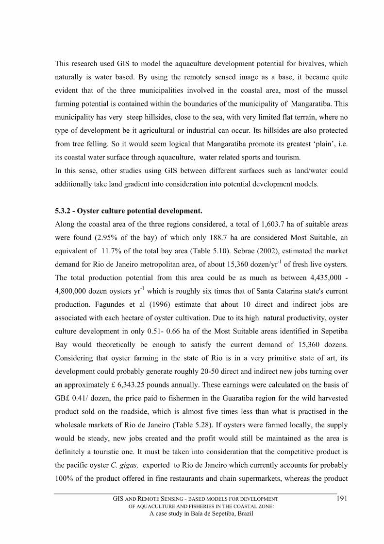
This research used GIS to model the aquaculture development potential for bivalves, which

naturally is water based. By using the remotely sensed image as a base, it became quite

evident that of the three municipalities involved in the coastal area, most of the mussel

farming potential is contained within the boundaries of the municipality of Mangaratiba. This

municipality has very steep hillsides, close to the sea, with very limited flat terrain, where no

type of development be it agricultural or industrial can occur. Its hillsides are also protected

from tree felling. So it would seem logical that Mangaratiba promote its greatest ‘plain’, i.e.

its coastal water surface through aquaculture, water related sports and tourism.

In this sense, other studies using GIS between different surfaces such as land/water could

additionally take land gradient into consideration into potential development models.

5.3.2 - Oyster culture potential development.

Along the coastal area of the three regions considered, a total of 1,603.7 ha of suitable areas

were found (2.95% of the bay) of which only 188.7 ha are considered Most Suitable, an

equivalent of 11.7% of the total bay area (Table 5.10). Sebrae (2002), estimated the market

demand for Rio de Janeiro metropolitan area, of about 15,360 dozen/yr

The total production potential from this area could be as much as between 4,435,000 -

4,800,000 dozen oysters yr es that of Santa Catarina state's current

production. Fagundes et al (1996) estimate that about 10 direct and indirect jobs are

associated with each hectare of oyster cultivation. Due to its high natural productivity, oyster

culture development in only 0.51- 0.66 ha of the Most Suitable areas identified in Sepetiba

Bay would theoretically be enough to satisfy the current demand of 15,360 dozens.

Considering that oyster farming in the state of Rio is in a very primitive state of art, its

development could probably generate roughly 20-50 direct and indirect new jobs turning over

an approximately £ 6,343.25 pounds annually. These earnings were calculated on the basis of

GB£ 0.41/ dozen, the price paid to fishermen in the Guaratiba region for the wild harvested

product sold on the roadside, which is almost five times less than what is practised in the

wholesale markets of Rio de Janeiro (Table 5.28). If oysters were farmed locally, the supply

would be steady, new jobs created and the profit would still be maintained as the area is

definitely a touristic one. It must be taken into consideration that the competitive product is

the pacific oyster C. gigas, exported to Rio de Janeiro which currently accounts for probably

100% of the product offered in fine restaurants and chain supermarkets, whereas the product

-1 of fresh live oysters.

-1 which is roughly six tim



191

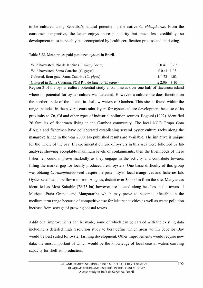
to be cultured using Sepetiba’s natural potential is the native C. rhizophorae. From the

consumer perspective, the latter enjoys more popularity but much less credibility, so

development must inevitably be accompanied by health certification process and marketing.

Table 5.28. Mean prices paid per dozen oysters in Brazil. Wild harvested, Rio de Janeiro (C. rhizophorae) £ 0.41 – 0.62 Wild harvested, Santa Catarina (C. gigas) £ 0.41- 1.03 Cultured, farm-gate, Santa Catarina (C. gigas) £ 0.72 - 1.03 Cultured in Santa Catarina, FOB Rio de Janeiro (C. gigas) £ 2.06 – 3.10

Region 2 of the oyster culture potential study encompasses over one half of Itacuruçá island

where no potential for oyster culture was detected. However, a culture site does function on

the northern side of the island, in shallow waters of Gamboa. This site is found within the

range included in the several constraint layers for oyster culture development because of its

proximity to Zn, Cd and other types of industrial pollution sources. Begossi (1992) identified

26 families of fishermen living in the Gamboa community. The local NGO Grupo Gota

d’Água and fishermen have collaborated establishing several oyster culture racks along the

mangrove fringe in the year 2000. No published results are available. The initiative is unique

for the whole of the bay. If experimental culture of oysters in this area were followed by lab

analyses showing acceptable maximum levels of contaminants, then the livelihoods of these

fishermen could improve markedly as they engage in the activity and contribute towards

filling the market gap for locally produced fresh oysters. One basic difficulty of this group

was obtaing C. rhizophorae seed despite the proximity to local mangroves and fisheries lab.

Oyster seed had to be flown in from Alagoas, distant over 3,000 km from the site. Many areas

identified as Most Suitable (78.75 ha) however are located along beaches in the towns of

Muriqui, Praia Grande and Mangaratiba which may prove to become unfeasible in the

medium term range because of competitive use for leisure activities as well as water pollution

increase from sewage of growing coastal towns.

Additional improvements can be made, some of which can be carried with the existing data

including a detailed high resolution study to best define which areas within Sepetiba Bay

would be best suited for oyster farming development. Other improvements would require new

data, the most important of which would be the knowledge of local coastal waters carrying

capacity for shellfish production.



192

5.3.3 - Shrimp culture potential development

The results of multi-criteria evaluation for the shrimp farming model predicted the outcome

illustrated in Figure 5.19. In the study area, two principal potential regions emerge, one

slightly separated from the other by the Santa Cruz-Campo Grande urban complex. In the

final analyses, consideration was given only to those areas classified as Most Suitable and

Suitable. Table 5.29 summarises the findings of the shrimp model.

Fig. 5.19. Regions in Sepetiba identified with significant shrimp culture potential.

Suitable

Table 5.29. Potential suitable shrimp cultivation sites. Most Suitable Moderately Suitable

Sepetiba study area 1,507 9,260 15,453 1315 5336 -

Guaratiba area 170 3640 Itaguaí area

- Region 1. - This study revealed two regions showing good potential for shrimp culture: The

larger potential is in Itaguaí, with 1,315 ha evaluated as Most Suitable. Figure 5.20 shows a

close up of this region in the area south of the interstate BR–101 which connects Rio to São

Paulo via the coast. The results of the MCE modelling indicate 255 hectares of area classified

as Most Suitable to the west of the Canal de São Francisco and another 1,061 ha to the east of

the canal. During the ground truthing part of this research both areas were visited. The first

area (a) (Fig. 5.20) possesses all the qualities for a good shrimp farming development, but is

in fact very close the industrial zone, which raises some concern as to the potential hazard



193

these activities may pose to a potential shrimp farm in operation. This area is probably already

precluded from agricultural development as it is zoned preferential for industrial activities.

The second area (b) adjacent (Fig 5.20), is ecologically very similar to the first, however

definitely zoned as agricultural land. A visit done in January 2003 revealed that part of the

area encompassing 900 ha, adjacent to the canal with a seafront is currently semi-abandoned

farmland, being claimed for settlement by members of the MST (Movimento dos Sem Terra)

from the federal government. Although the land could probably be used for shrimp farming,

there are questions such as for how long the water quality in the area will remain adequate for

the activity, taking into consideration the steady growth rate of Itaguaí and Santa Cruz and the

poor history of sewage treatment in the state of Rio. On the positive side, The location of

these areas in region 1, could hardly be better in terms of access to roads, proximity to

conducive ecosystems for shrimp growth, sources of fresh and seawater, local and export

markets among other production factors analysed in this model.

An interesting finding about these two regions is the percentage of the area covered by each

suitability class. While in the Itaguaí region the area classified as Most Suitable covers 19.8%

of the classes Most Suitable and Suitable, totalling and area of 6,651 ha, in Guaratiba this

percentage falls to 4.5% of a total area of 3,810 ha. This shows that region 1 has a larger Most

Suitable area, more ‘safely embedded’ in a larger Suitable area, and can possibly indicate

higher stability of the shrimp farming conditions regime, hence being considered more

propitious for development.



194

Fig. 5.20 Suitable areas for shrimp farming in the Itaguaí region of Sepetiba Region 2. – Figure 5.21 shows the second region identified by the model, Guaratiba, which in

fact is the birthplace of shrimp farming in Brazil carried experimentally by British American

Tobacco Co, (Cia. Souza Cruz) in the early seventies. The first shrimp ponds were built just to

the east of Pedra de Guaratiba a fishing village and the mangroves of Guaratiba. The region

nowadays is considerably protected from industrial development, the scenery dominated by

farmland, mangrove canals and salt barrens and tend towards tourism development. To date,

the FIPERJ fisheries lab is active, and could be used to bolster the region’s economic

performance with a sustainable use of the environment such as shrimp aquaculture. Producing

aquaculture research, seed and disseminating expertise is its mission statement, so this is a

significant advantage of any potential site close to the station. Nonetheless, a close-up GIS-

assisted investigation would be needed in order to verify in-depth actual land availability and

other conditions. This could be done with the use of aerial photos on a larger scale than was

attempted in this research.

Fig. 5.21 Suitable areas for shrimp farming in the Guaratiba region of Sepetiba.



195

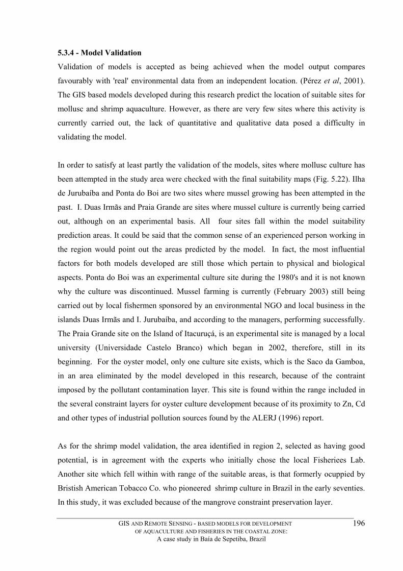
5.3.4 - Model Validation

Validation of models is accepted as being achieved when the model output compares

favourably with 'real' environmental data from an independent location. (Pérez et al, 2001).

The GIS based models developed during this research predict the location of suitable sites for

mollusc and shrimp aquaculture. However, as there are very few sites where this activity is

currently carried out, the lack of quantitative and qualitative data posed a difficulty in

validating the model.

In order to satisfy at least partly the validation of the models, sites where mollusc culture has

been attempted in the study area were checked with the final suitability maps (Fig. 5.22). Ilha

de Jurubaíba and Ponta do Boi are two sites where mussel growing has been attempted in the

past. I. Duas Irmãs and Praia Grande are sites where mussel culture is currently being carried

out, although on an experimental basis. All four sites fall within the model suitability

prediction areas. It could be said that the common sense of an experienced person working in

the region would point out the areas predicted by the model. In fact, the most influential

factors for both models developed are still those which pertain to physical and biological

aspects. Ponta do Boi was an experimental culture site during the 1980's and it is not known

why the culture was discontinued. Mussel farming is currently (February 2003) still being

carried out by local fishermen sponsored by an environmental NGO and local business in the

islands Duas Irmãs and I. Jurubaíba, and according to the managers, performing successfully.

The Praia Grande site on the Island of Itacuruçá, is an experimental site is managed by a local

university (Universidade Castelo Branco) which began in 2002, therefore, still in its

beginning. For the oyster model, only one culture site exists, which is the Saco da Gamboa,

in an area eliminated by the model developed in this research, because of the contraint

imposed by the pollutant contamination layer. This site is found within the range included in

the several constraint layers for oyster culture development because of its proximity to Zn, Cd

and other types of industrial pollution sources found by the ALERJ (1996) report.

As for the shrimp model validation, the area identified in region 2, selected as having good

potential, is in agreement with the experts who initially chose the local Fisheriees Lab.

Another site which fell within with range of the suitable areas, is that formerly ocuppied by

Bristish American Tobacco Co. who pioneered shrimp culture in Brazil in the early seventies.

In this study, it was excluded because of the mangrove constraint preservation layer.



196

5.3.5 - Shrimp farming potential development

Fig. 5.22. Location of several actual mollusc culture sites within the sites predicted by the models.

Accordng to Scott et al 2002, the estimated annual market consumption of shrimp for the Rio

de Janeiro both wholesale and retail is estimated to be 528 tons per year. As shown in Table

5.30, if the region were to develop shrimp farming in order to meet current detected shrimp

demand, it would only to develop 234.7 ha of farmland area. The actual shrimp pond surface

needed is 176 ha. In practice, a 25% margin of land is left available within a shrimp

development project for allocation to construction of pond dikes, service buildings and

maneuvering areas. This area (234.7 ha) is equivalent to only 15.8% of the Most Suitable

areas found in both region 1 and region 2. Table 5.30. Summary of potential development implications in study area.

Most Suitable areas (ha) detected in Study area, (Region 1 & 2) 1,485 Land surface area allocated for pond construction, buildings and maneuvering areas (%)

25

Estimated shrimp consumption of Rio de Janeiro tons/yr 528 Estimated productivity (tons/ ha / year ) 3 Area (ha) to be developed to meet detected demand 234.7



197

In economical terms, it is important to note that Rio de Janeiro is currently a major importer

of fresh shrimp, most of it originating from aquaculture activities carried out in the

northeastern states of Brazil, mainly Rio Grande do Norte, Ceará and Bahia. The market

standard specimen is a 12 g white shrimp of the species Litopenaeus vannamei. Prices paid

by the wholesaler at the farm gate are currently about R$ 7/kg or about £1.30/kg at the current

exchange rate (April, 2003). By checking with experienced consultants in the shrimp farming

business, it was found that the construction cost per hectare of built shrimp pond is estimated

to be between 10,000 to US$ 15,000. Table 5.31 summarises the investment needed to build

enough pond area in order to meet the Rio de Janeiro state demand for shrimp as well as the

potential gross earnings from such an aquaculture industry if installed in the Sepetiba area.

Table 5.31 Summary of study area potential for shrimp farming.

Shrimp production target Rio state demand) (t/yr) 528 0.012 1.30

Investment needed GB£/ha 9,166.67 1,613.333.33 684,844.44

3,341

Shrimp average size Kg Average farm gate price GB£/ kg

Investment needed to meet demand GB£ Gross earnings by meeting state demand GB£ Total potential production of the study area (t/yr)

Since the detected production potential of the study area is about 6.3 times greater than the

current demand in Rio de Janeiro, developing all the areas identified as Most Suitable for

shrimp aquaculture (1,485 ha) can go further than just meet demands from local markets but

also become a respectable sector of agribusiness with potential to satisfy demands of

neighbouring states such as São Paulo and Minas Gerais or alternatively foreign markets.

Among the benefits of developing this shrimp farming potential, is the creation of 2 jobs per

hectare of shrimp pond, and the transformation of the decadent agricultural production

scenario of the region into a more dynamic activity. Production can be easily trucked to

processing plants and wholesale markets in Rio at a much lower cost than that of production

sites found in northeastern Brazil.



198

CHAPTER 6.

GENERAL DISCUSSION

The purpose of this study was to investigate the use of GIS supported by Remote Sensing, to

predict promising locations for coastal aquaculture development. If natural indicators of

biological productivity and other aquaculture production functions could be assembled into a

GIS, what would be the production potential and economic consequences of this development

in terms of job creation and natural resource exploitation ?

Two species of filter feeding molluscs were chosen for this investigation in an attempt to

answer these questions:

1. the marine brown mussel Perna perna found in tropical and subtropical

environments in the Atlantic; and

2. the estuarine Crassostrea rhizophorae a mangrove oyster found commonly from

the Carribean to the warmer latitudes of southern Brazil.

3. the exotic marine shrimp Litopenaeus vannamei the most cultured shrimp

throughout all latitudes in Brazil

Commercial filter-feeding molluscs were chosen because they are sessile organisms,

dependent on the general quality of the aquatic environment in which they live, and support

verification of the prediction models developed in this research. They also have a well

established market value allowing for economic analyses of the potential assessed. The exotic

marine shrimp was chosen because it is now the most important commercial shrimp species

which has a wide tolerance of environmental ranges and is a commodity in high demand.

The region of Sepetiba Bay, Rio de Janeiro was chosen for this investigation in an attempt to

answer these questions. Generally, coastal oceanographic data is very scarce, and Rio de

Janeiro is no exception. An underdeveloped local aquaculture industry needs orientation on

site suitability and potential economic benefit derived from it.



199

The main approach of this work was to study the interaction of environmental, physical,

infrastructural and market parameters developed as independent layers in a GIS environment

integrated in a model which would simulate the best conditions for siting a bivalve mollusc

cultivation installation satisfying a set of aquaculture development criteria.

Area extent for mussel and oyster cultivation was determined using the base raster Landsat

image and the outcome layers of the production function sub-models integrated in a final

multi-criteria evaluation (MCE). The potential of aquaculture development for the region of

Sepetiba was thus determined for Perna perna and Crassostrea rhizophorae using the

biological data available. On the landsaide of Sepetiba bay, aquaculture development potential

was determined in a similar way using a diferent model for Litopenaeus vannamei. Also

estimates of potential returns from aquaculture exploitation of these three species was

attempted, taking into consideration the current market consumption estimate for metropolitan

Rio de Janeiro.

The first step was to try to understand how the species considered are related naturally to their

growing environment. A set of thematic layers including water surface salinity, dissolved

oxygen and temperature were setup in the GIS, using a remotely sensed image (Landsat 5) as

a backdrop. The backdrop image in raster format served as a base for further integrated

analyses.

For the analyses of the site suitability for aquaculture development of three species, sub-

models were developed taking into consideration different production functions. This was

because water quality parameters, infrastructural support, physical factors associated with the

production structures, and market aspects vary spatially.

The first opportunity to work in Sepetiba with mussel culture experiments over a wide range

was in 1996, where experimental cultivation ropes were placed in a series of positions across

the bay hoping to follow their development in time and use these as controls for the models

developed during the research. Unfortunately, these controls were removed by the local

population, but the exercise served to collect site specific information useful to verify proxy

data developed and maps used as layers in the GIS.



200

The main objective of using GIS in the project was to test its capacity as a tool to find new

development sites.

Field work, based on several map sources helped in obtaining a clearer picture of the spatial

variability of environmental parameters in this dynamic coastal area. The opportunity to work

aboard the R/V Úrsula in 1998 collecting samples from the study area was particularly

important and served to feed the GIS database for Sepetiba. The results suggest that there is

significant bivalve mollusc and penaeid shrimp aquaculture potential that could be developed

in the region even though it is considered by many as very inappropriate because of the

perceived pollution from the hydrographic basin attached to this coastal protected area. In this

context, GIS is very useful as it can be very objective giving results based on a series of

criteria (MCE) carefully selected and weighed by a wide range of professionals on the subject

matter, culminating in a clear evaluation, rather than ‘expert opinion’ which many times is

biased or unfamiliar with different conditions present over wide geographical areas resulting

in unrealistic ratings for a specific site.

From the analysis of the GIS prediction model it was clear that a majority of the bay´s waters

are in fact inappropriate for mussel or oyster farming because of the pollution constraint, but

also because of other constraints not relative to pollution or important from the human

consumption aspect of the aquaculture production, such as conflicting activities in navigation,

fisheries and military use.

It was also possible to develop a significant wave height prediction submodel in the GIS,

which gave the physical factors sub-model (shelter) the extra credibility needed for

integration into the general model.

In an attempt to interpret the waters’ suitability as natural productivity (an indication of

mollusc bivalve food availability), another technique was developed and experimented in this

research which was the use of a Chlorophyll a determination algorythm to develop a thematic

layer for integration into the general model, using this ‘instantaneous’ data available and

historical data in the form of Chlorophyll a cartograms published by FEEMA. This type of

integration into a mollusc suitability model could highly benefit from images available from

the SeaWifs satelite, specialised in ocean colour interpretation.



201

Conclusions and directions for further research

1. MCE in the GIS proved to be an important tool for weighing impressions of

professionals from different fields of expertise, all with different angles of perception

about the various aquaculture production functions. The ‘expert panel’ assembled in

this research added an ecletic component into the GIS which resulted in a narrowing

down of potential sites to a minimum. Consensus even between experts in the same

field was low, so that weights developed for production functions varied considerably.

Interviews with professionals for developing weights to be used in MCE should be

done very carefully.

2. A considerable area of the bay was classified as Most Suitable for the cultivation of

Perna perna and Crassostrea rhizophorae in Sepetiba Bay. However, the amount of

heavy metals retained in the tissues of cultivated organisms for the period of culture

(about 8 - 12 months) under the prevailing conditions is unknown. Possibly, there

could be a build-up which is still at allowable levels for human consumption. This

assessment should be attempted and compared with the levels in wild stocks currently

harvested. Area classification for health safety would be thus achieved and give

consumer confidence necessary and as a result industry growth.

3. The sites identified as Most Suitable for both mollusc and shrimp cultivation in many

cases match with sites where experimental, recent or not, cultivation has been

attempted. Success rate at these sites should be followed up together with a study of

the intuitive processes which led the entrepreneurs to choose these sites and see how

they fit in the AHP weighting process.

4. Perna perna and Crassostrea rhizophorae are two species which are characterised by

living in quite distinct environmental regimes. This on one hand facilitated the spatial

analyses carried out in this research. Further GIS aquaculture modelling in this type of

coastal environment could benefit from incorporating a third species such as

Anomalocardia brasiliana a venerid clam, which thrives in an intermediate habitat

between the mangroves and the marine rocky outcrops. While both P.perna and C.

rhizophorae feed on plankton, A. brasiliana depends mostly on microphytobenthos for



202

its nutrition. However due to the restrictions of time and resources the incorporation of

this third species in the modelling exercises was not attempted. It could prove an

interesting new study opportunity, especially if supported by SeaWifs imagery.

5. Although information about bottom sediment quality and water colour were available,

they were not integrated in the mollusc suitability model. However, bottom sediment

particle size could be an important information inasmuch as it can contribute to a layer

which describes the water velocity in the bay.

The work presented in this thesis provides a significant contribution to the use of GIS in

aquaculture site selection in the coastal environment. It has shown that better coverage of the

data is necessary to assess fully this potential. It is essential to have control sites with actual

mollusc cultivation in order to evaluate actual growth under the prevailing conditions and

ultimately, to relate this to the development of carrying capacity assessment of the region so

as to best manage and support development of aquaculture industry.



203

Literature Cited

Acuna, C.A. (1977) Crecimiento y indice de engorda del mejillon Perna perna (L.) cultivado en el Golfo de Cariaco, Venezuela. Report 200, pp. 1-9.

AGI. (99) Association for Geographic Information (AGI). http://www.agi.org.uk/

Aguilar-Manjarez, J. and Nath, S.S. (1998) A strategic reassessment of fish farming potential in Africa., CIFA - Technical Paper Rome: FAO. vol. 32, 170 p.

Aguilar-Manjarrez, J. (1996) Development and evaluation of GIS-based models for planning and management of coastal aquaculture: A case study in Sinaloa, Mexico. PhD Thesis, University of Stirling. Stirling, Scotland. 373 p.

Aguilar Manjarrez, J. and Ross, L.G. (1993) Aquaculture development and GIS. Mapping-Awareness-and-GIS-in-Europe. vol. 7 (no. 4), pp. 49-52.

ALERJ (1996) Contaminação ambiental da Baía de Sepetiba pela Companhia Mercantil e Industrial INGA. Comissão de Meio Ambiente da Assembléia Legislativa do Estado do Rio de Janeiro. Rio de Janeiro. 25 p.

Ali, C.Q., Ross, L.G. and Beveridge, M.C.M. (1991) Microcomputer spreadsheets for the implementation of geographic information systems in aquaculture: A case study on carp in Pakistan. AQUACULTURE. vol. 92 (no. 2-3), pp. 199-205.

Anonymous (1995) Santa Catarina: A padroeira das ostras e mexilhões.Panorama da Aqüicultura. vol. 5 (no. 30), pp. 12-21.

Ariz, J., Delgado de Molina, A., Santana, J.C., Arbelo, M., Hernandez and P.Herrera, F. (unpublished) Relación entre las capturas de patudo Thunnus obesus (Lowe, 1839), la temperatura superficial y diversos fenómenos mesoescalares, mediante el uso de teledetección en el área de las Islas Canárias durante 1994. In press

Baban, S.M.J. (1997) Environmental monitoring of estuaries: estimating and mapping various environmental indicators in Breydon Water Estuary, U.K., using Landsat TM imagery. ESTUAR.-COAST.-SHELF-SCI. vol. 44 (no. 5), pp. 589-598.

Bagheri, S. and Dios, R.A. (1990) Chlorophyll-a estimation in New Jersey's coastal waters using Thematic Mapper data. INT.-J.-REMOTE-SENS. vol. 11 (no. 2), pp. 289-299.

Barg, U. (1992) Guidelines for the promotion of environmental management of coastal aquaculture development. FAO - fisheries technical paper Rome: FAO. vol. 328, 122 p.

Barroso, G & Bonetti Filho. (2002) Planning of shelfish farming in a tropical estuary: a spatial analysis approach..In: Second International Symposium on GIS/Spatial Analyses in Fishery and Aquatic Sciences. 3-6 September, 2002 University of Sussex, Brighton, United Kingdom. pp. 64 .



204

Begossi, A. (1992) The Use of Optimal Foraging Theory in the Understanding of Fishing Strategies: A Case from Sepetiba Bay (Rio de Janeiro State, Brazil).Human Ecology vol. 20 (no. 4), pp. 463-475.

Begossi, A. (1995)Fishing spots and sea tenure: incipient forms of local management in Atlantic forest coastal communities. Human-Ecology. vol. 23. (3): pp. 387-406.

Begossi, A. and de Figueiredo, J.L. (1995) Ethnoichthology of Southern Coastal Fishermen: Cases from Búzios Island and Sepetiba Bay (Brazil).Bulletin of Marine Science vol. 56 (no. 2), pp. 710-717.

Beveridge, M. C. (1996) Cage Aquaculture. England: Fishing News Books; 352 p.

Bompais, X. (1991) Les filières pour l'elevage des moules., France. 249 p.

Bonetti Filho, J., Beltrame, E. $ Bonetti, C. (2002) Integration of hydrological index and Gis for shrimp culture in subtropical Brazilian coast., In: Second International Symposium on GIS/Spatial Analyses in Fishery and Aquatic Sciences. Abstracts. Fishery/Aquatic GIS Research Group. 3-6 September, 2002 University of Sussex, Brighton, United Kingdom. pp. 63 ..

Braga, C.Z.F., Setzer, A.W. and de Lacerda, L.D. (1993) Water quality assessment with simultaneous Landsat-5 TM data at Guanabara Bay, Rio de Janeiro, Brazil. REMOTE-SENS.-ENVIRON. vol. 45 (no. 1), pp. 95-106.

Burrough, P.A. and McDonnell, R.A. (1998) Principles of Geographical Information Systems., First edn. Oxford, UK: Oxford University Press. 333 p.

Caddy, J.F. and Griffiths, R.C. (1995) Living marine resources and their sustainable development., FAO - fisheries technical paper. Rome: FAO. vol. 353, 167 p.

Cansado-Marrero, S. (1998) Assessment of mollusc culture potential in Baía de Sepetiba, Brazil. A GIS-Based model. University of Stirling. Stirling, Scotland 71 p.

Carvalho, C.E.V., de Lacerda, L.D. and Gomes, M.P. (1991) Heavy metal contamination of the marine biota along the Rio de Janeiro coast, SE-Brazil. Water, Air, and Soil Pollution vol. 57-58, pp. 645-653.

Carvalho, C.E.V.d.L.L.D.a.G.M.P. (1993) Metais pesados na biota bêntica da Baía de Sepetiba e Angra dos Reis, RJ.Acta Limnologica Brasiliensia. vol. 6, pp. 222-229.

Casabellas, M.A.C. (1991) Depuración de Moluscos. Galícia, Spain: Consillería de Pesca. 58p.

CDRJ (1999) Porto de Sepetiba. http://www.transportes.gov.br/denys/pbea/pbsepe.htm.

Chacon Torres, A., Ross, L.G., Beveridge, M.C.M. and Watson, A.I. (1992) The application of SPOT multispectral imagery for the assessment of water quality in Lake Patzcuaro, Mexico. INT.-J.-REMOTE-SENS. vol. 13 (no. 4), pp. 587-603.



205

CIDE - Centro de Informações e Dados do Rio de Janeiro. (2000) Anuário Estatístico do Rio de Janeiro 199 - 2000. Rio de Janeiro: Secretaria de Planejamento do Rio de Janeiro. CD-ROM.

Clark, C.D. (1993) Satellite remote sensing of marine pollution. International Journal of Remote Sensing vol. 14 (no. 16), pp. 2985-3004.

Clark, J.R. (1992) Integrated Management of Coastal Zones., FAO - fisheries technical paper Rome: FAO. vol. 327, 167 p.

CNES-IFREMER (1987) The preselection of sites favourable for tropical shrimp farming. Rome, Italy: FAO. FAO - Fisheries Technical paper vol. 318.

CONAMA (1986) NT-202. R-10 Critérios e padrões para lançamento de efluentes líquidos. 5p.

Costa, M. F. P, Galvão, S. M. G., and Novo, E. M. L. N. (1998) Quantificação espacial de clorofila-a na água do mar utilizando dados do sensor TM/Landsat-5: região costeira de Ubatuba, SP. IX Simpósio Brasileiro de Sensoriamento Remoto, Santos, SP. 12 p.

de Lacerda, L.D., de Carvalho, C.E.V. and Gomes, M.P. (1989) Nota sobre a distribuição de Mn, Zn, e Cu em sirís da Baía de Sepetiba. Rev. Bras. de Biol. vol. 49 (no. 3), pp. 847-849.

de Lacerda, L.D. and de Rezende, C.E. (1986) Metals in the Seagrass Halodule wrightii Aschers during one growing season. Revta brasil. Bot vol. 9, pp. 87-90.

de Lacerda, L.D.d., Lima, N.R.W., Pfeiffer, W.C. and Fiszman, M. (1983) Size and metal concentration in the mangrove mussel Mytella guyanensis (Mollusca: Bivalvia) from Baía de Sepetiba, Brazil. Rev. Biol. Trop. vol. 31 (no. 2), pp. 333-335.

de Rezende, C.E. and de Lacerda, L.D. (1986) Metais Pesados em Mexilhões (Perna perna L.) no litoral do Estado do Rio de Janeiro. Rev. Bras. Biol. vol. 46 (no. 1), pp. 239-247.

DeMers, M.N. (1997) Fundamentals of Geographic Information Systems. U.S.: John Wiley & Sons. 486 p.

Dib, A.K. (1992) O transporte de sedimentos em suspensão e a concentração de metais pesados em sedimentos de fundo nos rios da Baixada de Sepetiba. Universidade Federal do Rio de Janeiro. 107 p.

Dudka, M. (1997) Precision Agriculture Initiative - Slide Show. http://rs320h.ersc.wisc.edu/ERSC/Projects/VIP/Precag/slides.html.

Eastman, R.J. (1997) Idrisi for Windows: Tutorial exercises. Eastman, R.J., (Ed.) MA, USA: 76 p.

Eastman, R.J. (1993) IDRISI - Technical Reference Manual. MA- USA: 213 p.



206

Eastman, R.J. (1997) IDRISI (USA) Manual. Worcester, MA: Clark University Graduate School of Geography. 213 p.

Fragoso, M.d.R. (1995) Estimativa do padrão de circulação da Baía de Sepetiba - RJ através de modelagem numérica. Universidade do Estado do Rio de Janeiro. Rio de Janeiro 37p.

Ekstrand, S. (1992) Landsat TM based quantification of chlorophyll-a during algae blooms in coastal waters. INT.-J.-REMOTE-SENS. vol. 13 (no. 10), pp. 1913-1926.

Fagundes, L., Henriques, M.B., Ostini, S. and Gelli, V.C. (1997) Custos e benefícios da mitilicultura em espinhel no sistema empresarial e familiar. Infornmações Econômicas. vol. 27 (no. 2), pp. 33-47.

Fagundes, L., Pereira, M., Henriques, M.B. and Eguchi, J.N. (1996) Aspectos Econômicos e produtivos na criação de ostra na região de Cananéia, Estado de São Paulo. Informações Econômicas. vol. 4, pp. 39-52.

FAO-Unesco (1971) Soil Map of the World. In Environmental Sciences - Bill Jamieson. Paris, France: UNESCO. vol. IV, 193 p.

FEEMA - Fundação Estadual de Engenharia do Meio Ambiente. (1997) Mapeamento dos Sedimentos da Baía de Sepetiba - Contaminação por Metais Pesados. Rio de Janeiro. 37 p.

FEEMA - Fundação Estadual de Engenharia do Meio Ambiente. (1993) A outra baía de problemas que o Rio não conhece: Baía de Sepetiba. Revista Feema ano II, no. 9 pp. 27-34.

FEEMA - Fundação Estadual de Engenharia do Meio Ambiente. (99) Projeto de Gerenciamento Costeiro do Estado do Rio de Janeiro. http://www.feema.rj.gov.br/fr-prog.htm

FEEMA - Fundação Estadual de Engenharia do Meio Ambiente. (1996) Termo de Referência 590. Rio de Janeiro. 19 p.

Ferguson, R.L. and Korfmacher, K. (1997) Remote sensing and GIS analysis of seagrass meadows in North Carolina, USA. Aquat.-Bot. vol. 58 (no. 3-4), pp. 241-258.

FIDERJ - Fundação Instituto de Desenvolvimento Econômico e Social do Rio de Janeiro. (1978) Indicadores Climatológicos do Estado do Rio de Janeiro. Rio de Janeiro. 156 p.

Flores-Nava, A. (1990) Water resources and freshwater aquaculture development of Yucatán, Mexico. University of Stirling. Stirling, Scotland. 388 p.

Folk, R. L. and Ward, W. C. (1957) Brazos River Bar: A Study in the Significance of Grain Size Parameters. Journal of Sed. Petrol. vol. 27:pp. 3-27.

Forster, B.C., Sha, X. and Xu, B. (1993) Remote sensing of sea water quality parameters using Landsat-TM. INT.-J.-REMOTE-SENS. vol. 14 (no. 15), pp. 2759-2771.



207

Fuchs, J., Martin, J.L.M. and Populus, J. (1998) Assessment of topical shrimp aquaculture impact on the environment in tropical aquaculture countries, using hydrobiology, ecology and remote sensing as helping tools for diagnosis. DRV/RA/RST/98-05, Paris, France. IFREMER. 262 p.

Garrison, T. (1999) Oceanography, An Invitation to Marine Science., Belmont, CA: Wadsworth . Trevor's book, 294. 552 p.

Geitner, Kerstin (2002) Use of GIS for Placement of Mariculture. In: Second International Symposium on GIS/Spatial Analyses in Fishery and Aquatic Sciences. 3-6 September, 2002 University of Sussex, Brighton, United Kingdom. pp. 92 .

GESAMP (1996) The contributions of science to integrated coastal zone management., Reports and studies. vol. 61 Rome, Italy: FAO. http://www.environment.gov.au/marine/manuals_reports/gesamp/gesamp_2.html

Goes, H.d.A. (1942) A Baixada de Sepetiba. MVOP - Departamento Nacional de Obras de Saneamento. 6 p.

Green, E.P., Mumby, P.J., Edwards, A.J. and Clark, C.D. (1996) A review of remote sensing for the assessment and management of tropical coastal resources.COAST.-MANAGE. vol. 24 (no. 1), pp. 1-40.

Grenier, M., Dubois, J-M. M., Lavoie, A., and Lambert, É. (1989) Télédétection de sites à potentiel aquicole dans la baie des chaleurs au Québec: résultats préliminaires. XII Symposium Canadien de Télédétection IGARSS, Vancouver, Canada. 4 p.

Gutierrez-Garcia, A. (1995) Development of a GIS-based socio-economic model for aquaculture development. University of Stirling. Stirling, Scotland. 84 p.

Haamer, J. (1996) Improving water quality in a eutrophied fjord system with mussel farming. AMBIO. vol. 5, pp. 356-362.

Habbane, M., El-SabhM.I. and Dubois, J.M. (1997) Potentiel aquacole regional par teledetection passive et SIG. International Journal of Remote Sensing. pp. 3439-3457.

Heral, M. (1991) Carrying capacity of shellfish ecosystems: Review of methods. THE-ECOLOGY-AND-MANAGEMENT-ASPECTS-OF-EXTENSIVE-MARICULTURE.-A-SYMPOSIUM-HELD-IN-NANTES,- 20-23-JUNE-1989. Lockwood,-S.J.-ed. vol. 192, pp. 48-62.

Hickman, R. W. (1992) The Mussel Mytilus: Ecology, Physiology, Genetics and Culture. Mussel Cultivation. London: Elsevier; vol. 25, pp. 465-510.

Ibrekk, H.O., Kryvi, H. and Elvestad, S. (1993) Nationwide assessment of the suitability of the Norwegian coastal zone and rivers for aquaculture (LENKA). COASTAL-MANAGE. vol. 21 (no. 1), pp. 53-73.

Idrisi Project. (2002) Idrisi Project - Homepage. http://www.clarklabs.org/IdrisiSoftware.asp?cat=2 2002.



208

Iversen, E.S. (1972) Cultivos Marinos - peces, moluscos y crustáceos., Zaragosa, Spain: Editorial Acribia. 312 p.

Jablonski, S., Du Mont, A.S. and Oliveira, J.S.d. (1997) O Mercado de Pescados no Rio de Janeiro. Montevideo, Uruguay. INFOPESCA. 79 p.

Jarayabhand, S. (1997) Management of coastal aquaculture in Thailand. University of Melbourne. Melbourne, Australia. 240 p.

Johannessen, J.A., Johannessen, O.M. and Haugan, P.M. (1988) Remote sensing and model simulation studies of the Norwegian Coastal current during the algal bloom in May 1988. Technical Report, Bergen, Norway. 16 p.

Junior, C. L. da S., Kampel, M., Araujo, C. E. S. de, Neto, O. O. de B., and Prieto, J. M. N. (1998) Imagens termais de satélite aplicadas à pesca de atuns e afins - Projeto SATPEIXE. IX Simpósio Brasileiro de Sensoriamento Remoto., 12 p.

Kapetsky, J.M. (1989) A geographical information system for aquaculture development in Johor State. FI:TCP/MAL/6754, Rome, Italy. FAO. 67 p.

Kapetsky, J.M. (1987) Satellite remote sensing to locate and inventory small water bodies for fisheries management and aquaculture development in Zimbabwe. Rome, Italy: FAO. CIFA Ocassional Paper, vol. 14 , 11 p.

Kapetsky, J.M. (1994) A strategic assessment of warm-water fish farming potential in Africa., CIFA Technical Paper FAO. vol. 27, 77 p.

Kapetsky, J.M., Hill, J.M. and Worthy, L.D. (1988) A geographical information system for catfish farming development. AQUACULTURE, vol. 68 (no. 4), pp. 311-320.

Kapetsky, J.M., Hill, J.M., Worthy, L.D. and Evans, D.L. (1990) Assessing potential for aquaculture development with a geographic information system. J.-WORLD-AQUACULT.-SOC. vol. 21 (no. 4), pp. 241-249.

Kapetsky, J.M., McGregor, L. and Nanne, H.E. (1987) A geographical information system and satellite remote sensing to plan for aquaculture development: A FAO-UNEP/GRID cooperative study in Costa Rica. FAO-FISH.-TECH.-PAP. vol. 287, 51 p.

Kapetsky, J.M. and Nath, S.S. (1997) A strategic assessment of the potential for freshwater fish farming in Latin America., FAO Copescal Technical Paper vol. 10 Rome, Italy.: FAO. 128 p.

Kapetsky, J.M., Wijkstrom, U.N., MacPherson, N., Vincke, M.M.J., Ataman, E. and Caponera, F. (1990) Ghana. Technical Assistance and Investment Framework for Aquaculture in Ghana. Field Technical Report 5. Where are the best Opportunities for Fish Farming in Ghana ? The Ghana Geographical Information System as a Decision-Making tool for fish Farming Development. Rome-Italy - FAO.

Karki, J. (1992) A Geographical Information System for hatchery developments in Nepal. University of Stirling. Stirling, Scotland. 47 p.



209

Kautsky, N., Berg, H., Folke, C., Larsson, J. and Troell, M. (1997) Ecological footprint for assessment of resource use and development limitations in shrimp and tilapia aquaculture. AQUACULT.-RES. vol. 28 (no. 10), pp. 753-766.

Krieger, Y. and Mulsow, S. (1990) GIS application in marine benthic resource management. GIS for the 1990s. - Proc. national conference, Ottawa, (CISM)., Ottawa, Canada. pp. 671-683.

Laing, I. and Spencer, B.E. (1997) Bivalve cultivation: criteria for selecting a site. Lowestoft, UK. CEFAS - Centre for Environment, Fisheries and Aquaculture Science. 41 p.

Lamego, A.R. (1964) O Homem e a Restinga., Rio de Janeiro, Brazil: Editora Lidador. 307 p.

Landau, M. (1992) Introduction to Aquaculture., first edn. New York, USA: John Wiley and Sons, Inc. 440 p.

Legault, J.A. (1992) Using a Geographic Information System to evaluate the effects of shellfish closure zones on shellfish leases, aquaculture and habitat availability. Using a Geographic Information System to evaluate the effects of shellfish closure zones on shellfish leases, aquaculture and habitat availability. 1882E, CAN.-TECH.-REP.-FISH.-AQUAT.-SCI. 14 p.

Lemos, M.B.N., Nascimento, I.A., de Araujo, M.M.S., Pereira, S.A., Bahia, I. and Smith, D.H. (1994) The combined effects of salinity, temperature, antibiotic and aeration on larval growth and survival of the mangrove oyster, Crassostrea rhizophorae. J. SHELLFISH RES. vol. 13 (no. 1), pp. 187-192.

Lima, N.R.W., de Lacerda, L.D.P.W.C. and Fiszman, M. (1986) Temporal and Spatial Variability in Zn,Cr,Cd and Fe Concentrations in Oyster Tissues (Crassostrea brasiliana Lamarck, 1819) From Sepetiba Bay, Brazil.Environmental Technology Letters. vol. 7, pp. 453-460.

Lo, C.P. (1991) Applied Remote Sensing., 2nd edn. New York, USA: Longman Scientific and Technical. 393 p.

Machado, M. C., Quiroga, A. I. P., and Tenório, M. B. (1998) Qualidade da água e biomassa fitoplanctônica de três ecosistemas marinhos com diferentes graus de eutrofização: Baía de Sepetiba e Litoral de Ipanema (Rio de Janeiro). Anais do IV Simpósio de Ecosisstemas Brasileiros, 2-7 abril 1998, Águas de Lindoya, SP, Brasil. vol. II, pp. 251-258 p.

Magalhães, A.R.M. and Ferreira, J.F. (1997) Mexilhões - Biologia e Cultivo. Universidade Federal de Santa Catarina. Florianópolis, Santa Catarina. 59 p.

Marques, H.L.d.A., Pereira, R.T.L. and Correa, B.C. (1991) Growth of mussels Perna perna [Linnaeus, 1758] in natural populations from Ubatuba shore, São Paulo State, Brazil. BOL. INST. PESCA SAO PAULO vol. 18, pp. 61-72.

Marques, H. L. de A; Pereira, R. T. L, and Correa, B. C. (1998) Seasonal variation in growth and yield of the brown mussel Perna perna (L.) cultured in Ubatuba, Brazil. Aquaculture 98, vol. 169 no. 3-4, p. 263-273.



210

Matsuura, Y. (1986) Contribution to the study of the oceanographic structure off the southeastern coast between Cabo Frio (RJ) and Cabo de Santa Marta Grande (SC). CIENC. CULT. SÃO PAULO. vol. 38 (no. 8), pp. 1439-1450.

Meaden, G.J. (1994) Background notes and prospects for a Libyan marine fisheries geographical information system. LIBFISH TECH. BRIEF. NOTES TRIPOLI LIBYA FAO: no. 3, 55 p.

Meaden, G.J. (1987) Where should trout farms be in Britain. Fish Farmer. March-April, pp. 33-35.

Meaden, G.J. and Do Chi, T. (1996) Geographical information systems. Applications to marine fisheries. Rome, Italy: FAO. FAO - Fisheries Technical Paper. vol. 356 , 335p.

Meaden, G. J. and Kemp, Z. (1997) Hancock, D.A., (Ed.) Monitoring fisheries effort and catch using a geographical information system and a global positioning system. World fisheries congress. Developing and sustaining world fisheries resources: The state of science and management, Brisbane, Australia Colinwood, Australia: CSIRO. 797 p.

Ministério do Meio Ambiente (1999) PROGRAMA NACIONAL DE GERENCIAMENTO COSTEIRO (GERCO). http://www.mma.gov.br/port/SMA/gerco/gerco.html.

Moreira, P. de C. da S. (1985) Manual de Maricultura. Rio de Janeiro, Brasil; 257 p.

Moura, J. A., Dias-Brito, D., and Bronnimann, P. (1982) Modelo Ambiental de Laguna Costeira Clástica-Baía de Sepetiba, RJ. IV Simpósio do Quaternário no Brasil. pp. 135-152p.

Nath, S.S., Bolte, J.P., Ross, L.G. and Aguilar-Manjarrez, J. (2000) Applications of Geographical Information Systems (GIS) for Spatial Decision Support in Aquaculture...Aquacultural Engeneering. vol. 23, pp. 233-278. .

Naylor, R.L., Goldburg, J., Mooney, H., Beveridge, M., Clay, J., Folke, C., Kautsky, N., Lubchenco, J., Primavera, J. and Williams, M. (1998) Nature's subsidies to shrimp and salmon farming.Science. vol. 282, pp. 883-884.

Oliveira, L.P.H. (1971) Prospecção hidrobiológica da Baía de Sepetiba.Memórias do Instituto Oswaldo Cruz. vol. 69 (no. 1), pp. 1-29.

Page, H.M. and Hubbard, D.M. (1987) Temporal and spatial patterns of growth in mussels Mytilus edulis on an offshore platform: Relationships to water temperature and food availability. .J.-EXP.-MAR.-BIOL.-ECOL. vol. 111 (no. 2), pp. 159-179.

Pattiaratchi, C., Lavery, P., Wyllie, A. and Hick, P. (1994) Estimates of water quality in coastal waters using multi-date Landsat Thematic Mapper data. INT.-J.-REMOTE-SENS. vol. 15 (no. 8), pp. 1571-1584.

Pauly, D., Gayanilo, F. and Jr. Silvestre, G. (1997) A low-level gepgraphic information system for coastal zone management, with applications to Brunei Darussalam: Part I: The concept and its design elements. NAGA vol. 20 (no. 2), pp. 41-45.



211

Paw, J. N., Diamante, D. A. D., Robles, N. A., Chua, T.-E., Quitos, L. N., and Cargamento, A. G. A. (1992) Site selection for brackishwater aquaculture development and mangrove reforestation in Lingayen Gulf, Philippines using geographic information system. Canadian Conference on GIS '92., Ottawa, Canada. pp. 821-832

Pereira, O.M., Akaboshi, S. and Soares, F.d.C. (1988) Cultivo experimental de Crassostrea brasiliana (LAMARCK, 1819) no canal de Bertioga, São Paulo, Brasil (23 54 30S 45 13 42 W).B. Inst. Pesca. vol. 15 (no. 1), pp. 55-65.

Pereira, O.M., Galvão, M.S.N. and Tanji, S. (1991) Época e método de seleção de sementes de ostra Crassostrea brasiliana (LAMARCK, 1819) no complexo estuarino - lagunar de Cananéia, Estado de São Paulo (25 S 048 W).B. Inst. Pesca, São Paulo, vol. 18 (único), pp. 41-49.

Perez-Martinez, O. 2002. GIS-based models for optimisation of marine cage aquaculture in Tenerife, Canary Islands. Ph.D thesis. University of Stirling. 2002.

Pérez, O. M., Telfer, T.C., Beveridge, M. C. M. anda Ross, L. G. (2002) Geograpical Information Systems (GIS) as a simple tool to aid modelling of particulate waste distribution at marine fish cage sites. Estuarine, Coastal and Shelf Science. vol 54, pp. 761-768.

Pérez, O. M., Telfer, T.C., Beveridge, M. C. M. anda Ross, L. G. (2002) Pptimización de la cuicultura marina de jaulas flotantes en Tenerife, Islas Canarias, mediante el uso de modelos basados en Sistemas de Información Geográfica (SIG) Revista AquaTIC, no 17.

Perez-Sanchez, E. 2002. Socio-economic assessment of small-scale aquaculture stakeholders in Tabasco, Mexico. Ph.D thesis. University of Stirling. 2002.

Rosman, P.C.C. (1998) Modelagem Computacional de Circulação Hidrodinâmica e Transporte de Contaminantes na Baía de Sepetiba, RJ. Rio de Janeiro, Brazil.

Pfeiffer W.C., de Lacerda, L.D., Fiszman, M., Rejane, N. and Lima, W. (1985) Metais Pesados no Pescado da Baía de Sepetiba, Estado do Rio de Janeiro RJ.Ciência e Cultura vol. 37 (no. 2), pp. 297-302.

Ponçano, W.L. (1976) Sedimentação Atual na Baía de Sepetiba, Estado do Rio de Janeiro. USP-Universidade de São Paulo. 42 p.

POND Biosystems Analysis Group - 1999. http://biosys.bre.orst.edu/pond/pond.htm.

Proença, C.E.M.d., Avelar, J.C. and Neto, F.M.d.O. (2001) Plataforma do Agronegócio da Malacocultura., 76 p.

Ramos, A.G., Santiago, J., Sangra, P. and Canton, M. (1996) An application of satellite-derived sea surface temperature data to the skipjack (Katsuwonus pelamis Linnaeus, 1758) and albacore tuna (Thunnus alalunga Bonaterre, 1788) fisheries in the north-east Atlantic. International-Journal-of-Remote-Sensing. vol. 17 (no. 4), pp. 749-759.

Rios, E.C. (1985) Seahells of Brazil., Rio Grande, RS: Museu Oceanográfico. 328 p.



212

Fundação COPPETEC - COPPE/UFRJ. 71 p.

Ross, L.G., Mendoza, E.Q.M. and Beveridge, M.C.M. (1993) The application of geographical information systems to site selection for coastal aquaculture: An example based on salmonid cage culture. AQUACULTURE. vol. 112 (no. 2-3), pp. 165-178.

Saaty, T.L. (1977) A scaling method for priorities in hioerarchical structures. Journal of Mathematics Physiology, vol 15, pp.234-281.

Saaty, T.L. (1995) Decision making for leaders: the Analytic Hierarchy Process for decision decision in a complex world., Pittsburgh, PA: RWS Publications.

Salam, A. Md. 2000. GIS modelling of coastal aquaculture development in Khulna district, Sunderbans, Bangladesh. Ph.D thesis. University of Stirling. 2000. p400.

Sathyendranath S. and Morel A. (1983) Light emerging from the sea-interpretation and its uses in remote sensing. In: Cracknell, A.P., (Ed.) Remote Sensing Applications in Marine Science and Technology. , Dordrecht; Boston: Lancaster. pp. 323-57.

Schurink, E.C.v. and Griffiths, C.L. (1992) Physiological energetics of four South African mussel species in relation to body size, ration and temperature. COMP.-BIOCHEM.-PHYSIOL. vol. 101A (no. 4), pp. 779-789.

Scott, P.C., Vianna, L.F. and Mathias, M.A.d.C. (2002) Diagnóstico da Cadeia Aqüícola para o Desenvolvimento da Atividade no Estado do Rio de Janeiro.Panorama da Aqüicultura. vol. 12 (no. 71), pp. 15-25.

SeaWiFS Project (1999) http://seawifs.gsfc.nasa.gov/SEAWIFS.html 99.

SEBRAE/ES - Serviço de Apoio às Micro e Pequenas Empresas do Espírito Santo. (1996) Programa Aquicultura - Relatório Final. Vitória-ES, Brazil. SEBRAE. 123 p.

SEBRAE/RJ - Serviço de Apoio às Micro e Pequenas Empresas no Estado do Rio de Janeiro Scott, P.C., Vianna, L.F. and Mathias, M.A.d.C., (Eds.) (2002) Diagnóstico da Cadeia Aqüícola para o Desenvolvimento da Atividade no Estado do Rio de Janeiro. Rio de Janeiro-RJ, Brazil. SEBRAE/RJ. 226 p.

SEMA - Secretaria de Estado de Meio Ambiente do Rio de Janeiro. CARTOGEO, NCE and UFRJ , (Eds.) (1996) Diagnóstico Ambiental da Bacia Hidrográfica da Baía de Sepetiba Projeto I. Projeto I., Rio de Janeiro, Brazil. 86 p.

Shahid, M.A. (1994) Application of remote sensing and GIS in shrimp farming areas of Bangladesh. SHORT-TERM-TRAINING-PROGRAMME-ON-GIS-FOR-FISHERIES,-14-18-NOVEMBER-1993 Ali,-A.;Mazid,-M.A.;Sinha,- V.R.P.-comp. 1994 pp. 102-109.

Shahid, M.A., Pramanik, M.A.H., Jabbar, M.A. and Ali, S. (1992) Remote sensing application to study the coastal shrimp farming area in Bangladesh. Geocarto-International. 1992. vol. 7 (no. 2), pp 5-13.

Shahid, M.A., Sayed, A., Tugril Hossain, T.I.M., Rahman, H., Sarker, M.H. and Ahmed, A.N.



213

(1997) Remote sensing and GIS for suitable shrimp farming area selection in Bangladesh.Journal of Remote Sensing and Environment. vol. 1, pp. 27-41.

Shumway, S.E. (1992) Mussels and Public Health. In: Anonymous The Mussel Mytilus: Ecology, Physiology, Genetics and Culture., London: Elsevier Developments in Aquaculture and Fisheries Science. Elizabeth Gosling pp. 511-542.

Signorini, S.R. (1980a) A Study of the Circulation in the Bay of Ilha Grande and Bay of Sepetiba* Part I - A Survey of the Circulation Based on Experimental Field Data.Bolm. Inst. Oceanogr., S.Paulo vol. 29 (no. 1), pp. 41-55.

Smith, G.F., Jordan, S.J. and Greenhawk, K.N. (1994) An oyster management information system: Integrating biological, physical, and geographical dimensions. J.-SHELLFISH-RES. vol. 13 (no. 1), 284 p.

Snedaker, S.C. and Getter, C.D. (1985) Coastal Management Publication. Coastal resources management guidelines. NPS/AID, Columbia, S. Carolina - USA. Research Planning Institute. 67 p.

Soletchnik, P., Le Moine, O., Faury, N., Razet, D., Geairon, P. and Goulletquer, P. (1999) Mortalité de l'huitre Crassostrea gigas dans le bassin de Marennes-Oléron: étude de la variabilité spatiale de son environnement et de sa biologie par un système d' informations geographiques (SIG).Aquat.Living Resour. vol. 12 (no. 2), pp. 131-143.

SUCOZOMA (1999) Sustainable Coastal Zone Management - SUCOZOMA - Revised Programme Plan 1999. 34 p. Sudarshana, R., Bhan, S.K., Siddiqui, M.S., Vohra, T.P.S., Prasad, P.N., Bhat, U.G. and Neelakantan, B. (1993) Experiments in site selection for coastal aquaculture using Indian remote sensing satellite: IRS-1A. INT.-J.-REMOTE-SENS. vol. 14 (no. 12), pp. 2275-2284.

Suguio, K. (1973) Introdução à Sedimentologia. Suguio, K. Introdução à Sedimentologia. São Paulo, Brasil: Edgard, Blücher;319 p.

Tait, R.V. (1981) Elements of Marine Ecology., London, UK.: Butterworths & Co. Publishers. 356 p.

Tassan, S. and Ribera d' Alcala, M. (1993) Water quality monitoring by thematic mapper in coastal environments. A performance analysis of local biooptical algorithms and atmospheric correction procedures. REMOTE-SENS.-ENVIRON. vol. 42 (no. 2), pp. 177-191.

Tomalin, B.J. (1995) Growth and mortality rates of brown mussels Perna perna (Linnaeus) in KwaZulu-Natal: A comparison between sites and methods using non-parametric length-based analysis. S.-AFR.-J.-MAR.-SCI.-S.-AFR.-TYDSKR.-SEEWET. vol. 16, pp. 241-254.

Tomas, J.E. and Cataldo de Castro, A.R. (1982) Atividades pioneiras de maricultura no Estado do Rio de Janeiro. Rio de Janeiro. Circular Técnica no. 5, 35 p.



214

UNITAR-United Nations Institute for Training and Research. (1995) Applications in coastal zone research and management., Explorations in Geographic Information Systems Technology vol. 3 Geneva, Switzerland.: UNITAR. vol. III, 141 P.

US Army Corps of Engineers (1984) Shore Protection Manual. Fourth edn, 1222 p. Washington, D.C: U.S. Government Printinting Office.

Vélez, A. and Epifanio, C.E. (1981) Effects of temperature and ration on gametogenesis and growth in the tropical mussel Perna perna (L)..Aquaculture vol. 22, pp. 21-26.

Wackernagel, M. and Rees, W. (1999) Our Ecological Footprint. http://www.ire.ubc.ca/ecoresearch/ecoftpr.html

Wakamatsu, T. (1973) A ostra de Cananeia e seu cultivo. São Paulo, Brazil. SUDELPA. 141 p.

Walne, P.R. (1979) Culture of Bivalve Molluscs., second edn. Farnham, Surrey - England: Fishing News Books Ltd. 189 p.



215

Appendix Appendix 1. List of co-ordinate pairs used to georeference Landsat satellite image based on admiralty chart 1622 produced by DHN. Sites Co-ordinates on

Landsat ‘Wind’ image

Co-

ordinates on

DHN chart

1622 Latitude degrees

min decimalminutes

Latitude degrees min decimal minutes

Converted to decimal degrees

for use in IDRISI

Converted to decimal degrees

for use in IDRISI

x y x y x yCais da Nuclep 696 898.9 -22.904 43 50 0.8 22 54 0.24 -43.8467 Campo Grande 1 1433.4 1061.9 43 37 0.58 22 53 0.5 -43.6263 -22.8917 Campo Grande 2 1468.9 1064.9 43 22 53 36 0.99 0.55 -43.6165 -22.8925 Campo Grande 3 1478.4 982.8 43 22 54 -22.9152 37 0 0.91 -43.6167 Canal de Sto Agostinho + linha de trem

1001.4 23 -23.8933 1005.7 43 44 0.6 53 0.6 -43.7433

Canal do Guandu 1 G1 981.4 840.6 43 55 -22.9317 45 0.95 22 0.9 -43.7658 Canal do Guandu 2 G2 1161.2 969.9 43 54 -23.905 42 0.6 23 0.3 -43.71 Canal do Ita 1 1063.6 803.9 43 22 56 44 0.78 0.73 -43.7463 -22.9455 Canal do Ita 2 1094.6 844.6 43 44 0.12 22 56 0.18 -43.7353 -22.9363 Canal do Ita 3 1213.2 961.9 43 41 0.7 22 54 0.5 -43.695 -22.9083 Coroa Grande, cais 631.3 879.5 43 52 0 22 54 0.4 -43.8667 -22.9067 From Lage M. to Afonso n 683.7 324.5 43 52 0.62 23 3 0.45 -43.877 -23.0575 From Lage M. to Afonso s 729 274.6 43 51 0.95 23 4 0.4 -43.8658 -23.0733 From Lage M. to Boca do Guandu 889.8 322.5 43 49 0.01 23 4 0.03 -43.8168 -23.0672 From Lage M. to Boca do Guandu 894.3 349.9 43 48 0.88 23 3 0.6 -43.8147 -23.06 From Lage M. to Boca do Ita 917.6 331.4 43 55 0 23 3 0.5 -43.9167 -23.0583 From Lage M. to Bonitinha 739.4 277 43 51 0.78 23 4 0.38 -43.863 -23.073

680.1 347.7 43 52 0.6 23 3 0.05 -43.8767 -23.0508



216

From Lage M. to Bonitinha

167

From Lage M. to Bonitinha 652.1 381.7 43 53 0.03 23 2 0.43 -43.8838 -23.0405 From Lage M. to Bonitinha 633.4 404.1 43 53 0.29 23 2 0.03 -43.8882 -23.0338 From Lage M. to Ilha Pescaria 917.5 330.9 43 47 0.6 23 3 0.8 -43.7933 -23.0633 From Lage M. to Ilha Pescaria 923.4 350.2 43 47 0.5 23 3 0.7 -43.7917 -23.0617 From Lage M. to Martins (E) 812.4 297.7 43 50 0.45 23 4 0.2 -43.8408 -23.07 From Lage M. to Martins (E) 812.5 297.2 43 50 0.58 23 3 0.19 -43.843 -23.0532 From Lage M. to Patio de Estocagem

852 310 43 49 0.73 23 49 0.73 -43.8288 -23.8288

From Lage M. to Patio de Estocagem

851.2 350.8 43 49 0.64 23 3 0.45 -43.8273 -23.0575

From Lage M. to Piracao 1353.9 445.4 43 40 0.8 23 3 0.25 -43.68 -23.0542 From Lage M. to Piracao 1522.5 550.06 43 37 0.55 23 2 0.99 -43.6258 -23.0498 From Lage M. to Porto Sepetiba (elbow)

832.7 4 303.4 43 50 0.08 23 0.19 -43.8347 -23.0698

From Lage M. to Porto Sepetiba (elbow)

825.9 353.9 43 50 0.8 23 3 0.35 -43.8467 -23.0558

From Lage M. to Pta Ferreiro 1170.7 399 43 43 0.99 23 3 0.5 -43.7332 -23.0583 From Lage M. to Pta Ferreiro 1181 407.9 43 43 0.79 23 3 0.4 -43.7298 -23.0567 From Lage M. to Pta Mangona N 513 297.9 43 55 0.6 23 3 0.4 -43.9267 -23.0567 From Lage M. to Pta Mangona S 627 243 43 53 0.8 23 4 0.65 -43.8967 -23.0775 From Lage M. to Pta. Grossa (Ita) 763.5 284 43 51 0.32 23 4 0.31 -43.8553 -23.0718 From Lage M. to Pta. Grossa (Ita) 700.4 382.4 43 52 0.2 23 2 0.55 -43.87 -23.0425 From Lage M. to Sai n 664.6 283.9 43 53 0.1 23 4 0.05 -43.885 -23.0675 From Lage M. to Sai s 691.7 263.1 43 52 0.65 23 4 0.49 -43.8775 -23.0748 From Lage M. to W Pta do Boi 789.6 291.5 43 50 0.85 23 4 0.03 -43.8475 -23.0671 From Lage M. to W Pta do Boi 758.3 366 43 51 0.2 23 2 0.99 -43.8533 -23.0498 From Pta Varejo Guandu 522.6 299 43 55 0.45 23 3 0.45 -43.9242 -23.0575 From Pta Varejo Guandu 614.1 408 43 53 0.55 23 1 0.95 -43.8925 -23.0325 From Pta Varejo to Bonitinha 56 3 -43.945 474.6 311.4 43 0.7 23 0.01 -23.0502 From Pta Varejo to Ilha Pescaria 584.1 288 43 54 0.44 3 23 0.8 -43.9073 -23.0633 From Pta Varejo to Ilha Pescaria 677 357 43 52 0.61 23 2 0.92 -43.8768 -23.0487 From Pta Varejo to Ilha Pescaria 709.4 381.2 43 51 0.99 23 2 0.62 -43.8665 -23.0437



217

168

From Pta Varejo to Ilha Pta Ipiranga

613 274 23 -23.0683 43 53 0.92 4 0.1 -43.8987


682.9 315 3 43 52 0.68 23 0.6 -43.878 -23.06


766.2 0.04 23 -43.8507 364 43 51 3 0.04 -23.0507

From Pta Varejo to Ita 550.6 23 0.5 300.3 43 55 0 3 -43.9167 -23.0583 From Pta Varejo to Ita 639 387.2 43 53 0.22 23 0.34 2 -43.887 -23.039

651.9 399.6 43 52 0.95 23 2 0.18 -43.8825 -23.0363 From Pta Varejo to Martins 795.7 358.2 43 56 0.3 23 3 0.13 -43.9383 -23.0522 Guaratiba (Ponta da Praia Funda) 1787 430.77 43 33 0.1 23 4 0.52 -43.5517 -23.0753 Hangar 01 da Aeronautica 1159.1 883.66 43 42 22 0.86 55 0.69 -43.7143 -22.9282Hangar 02 1138.3 843.7 43 43 0.35 22 56 0.3 -43.7225 -22.9383 Hangar 03 22 0.34 1129.9 775.8 43 43 0.6 57 -43.7267 -22.9557 Ilha Baleia (E) 35 1647.8 535 43 0.35 23 2 0.51 -43.5892 -23.0418 Ilha Bonita (N) 537.4 555.4 43 54 0.5 22 59 0.34 -43.9083 -22.989 Ilha Bonitinha (S) 528.35 527.47 43 54 0.75 22 59 0.8 -43.9125 -22.9967 Ilha da Bala, Centro 417 483.6 43 56 0.8 23 0 0.2 -43.9467 -23.0033 Ilha da Carapuca (N) 444.07 572.81 43 56 0.1 22 58 0.74 -43.935

574.32 795.65 43 53 0.22 22 55 0.4 -43.887 -22.9233 Ilha da Guaiba, Ponta (N) 117.3 463.7 44 2 0.4 22 0.75 59 -44.04 -22.9958 Ilha da Guaiba, Ponta (S) 83.021 405.15 44 2 0.84 23 0 0.6 -44.0473 -23.01 Ilha da Jurubaiba (W) 375.59 641.74 43 57 0.09 22 57 0.58 -43.9515 -22.9597 Ilha da Pescaria (S) 1168.1 722.88 43 43 0.131 22 58 0.35 -43.7189 -22.9725 Ilha da Sapioeira 609.26 813.51 43 52 0.55 22 55 0.42 -43.8758 -22.9237 Ilha da Vigia Grande (S) 57 23 -43.9525 43 0.15 0 0.55 -23.0092 Ilha da Vigia Pq (S) 393.05 481.59 -23.003 43 57 0.2 23 0 0.18 -43.9533 Ilha das 2 irmas (E) 333.3 696.6 43 57 0.78 22 56 0.55 -43.963 -22.9425 Ilha de Guaraquecaba (N) 1381 657.75 43 39 0.6 22 59 0.9 -43.66 -22.9983 Ilha de Jaguanum (W) 462.4 518.7 43 55 0.9 22 59 0.78 -43.9317 -22.9963 Ilha do Bernardo (S) 409.8 400.07 43 57 0.15 23 1 0.54 -43.9525 -23.0257

43 55 0.4 0.91 -43.9233

From Pta Varejo to Ita

-22.979 Ilha da Gamboa N

Ilha do Bicho Peq (N) 485.2 574.6 22 58



218

-22.9818

169

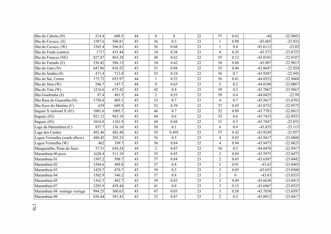
Ilha do Cabrito (N) 214.4 608.5 44 22 0.62 -44 0 0 57 -22.9603 Ilha do Cavaco, (S) 1587.6 560.81 -43.605 43 36 0.3 23 1 0.98 -23.033 Ilha do Cavaco, (W) 566.81 -43.6113 1565.4 43 36 0.68 23 1 0.8 -23.03 Ilha do Frade (centro) 1717 431.44 43 34 -43.573 -23.0725 0.38 23 4 0.35 Ilha do Frances (NE) 827.87 865.28 43 48 0.62 22 55 0.12 -43.8103 -22.9187

536.42 586.15 43 54 0.42 22 58 0.88 -43.907 -22.9813 Ilha do Gato (N) 647.86 816.52 43 51 0.88 22 55 0.44 -22.924 -43.8647 Ilha do Jardim (S) 471.4 713.4 55 43 0.24 22 56 0.7 -43.9207 -22.945 Ilha do Sai, Center 175.72 655.97 44 1 0.52 22 56 0.81 -44.0253 -22.9468 Ilha do Sino (W) 246.7 147.7 44 0 0.65 23 5 0.2 -44.0108 -23.0867 Ilha do Tatu (W) 1216.6 675.42 43 42 0.4 23 59 0.2 -43.7067 -23.9867 Ilha Guaibinha (S) 87.4 481.5 44 2 0.55 22 59 0.4 -44.0425 -22.99 Ilha Rasa de Guaratiba (N) 1756.6 405.1 43 33 0.7 23 4 0.7 -43.5617 -23.0783 Ilha Soco do Martins (C) 639 689.9 43 52 0.39 22 57 0.45 -43.8732 -22.9575 Itaguai X railroad X (01) 1001.6 1005.7 43 46 0.7 22 52 0.89 -43.7783 -22.8815 Itaguai, (02) 921.12 0.6 963.18 43 44 22 53 0.6 -43.7433 -22.8933Itaguai, (03) 1016.8 1101.9 43 44 0.68 22 51 0.3 -43.7447 -22.855 Lage da Marambaia (C) 857.7 136.18 43 50 0.1 23 6 0.9 -43.835 -23.115 Lage dos Cardos 492.46 482.48 55 0.495 23 57 0.42 -43.9249 -23.957 Lagoa Vermelha (south elbow) 480.45 205.23 43 56 0.5 23 4 0.85 -43.9417 -23.0808 Lagoa Vermelha (W) 462 199.7 43 56 0.84 22 4 0.94 -43.9473 -22.0823 Mangaratiba, Praia do Saco 37.51 656.24 44 2 0.87 22 56 0.5 -44.0478 -22.9417 Marambaia 00 poco 1620.4 511.19 43 35 0.85 22 2 0.84 -43.5975 -22.0473 Marambaia 01 1507.2 508.7 43 37 0.84 23 2 0.65 -43.6307 -23.0442 Marambaia 02 23 1504.6 488.8 43 37 0.8 2 0.91 -43.63 -23.0485Marambaia 03 1429.7 470.7 43 39 0.3 23 3 0.05 -43.655 -23.0508Marambaia 04 1502.9 546.2 43 37 0.8 23 2 0 -43.63 -23.0333Marambaia 05 1362.3 482.7 43 39 0.83 23 2 0.49 -43.6638 -23.0415 Marambaia 07 1285.9 439.44 43 41 0.8 23 3 0.15 -43.6967 -23.0525Marambaia 08 restinga verruga 994.25 0.03 360.63 43 47 23 3 0.58 -43.7838 -23.0597 Marambaia 09 656.44 381.43 43 52 0.87 23 2 0.5 -43.8812 -23.0417

Ilha do Furtado (E)

43



219

170

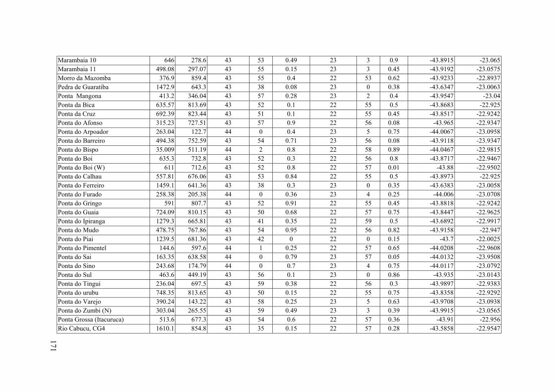
Marambaia 10 646 -43.8915 278.6 43 53 0.49 23 3 0.9 -23.065 Marambaia 11 498.08 297.07 43 55 0.15 23 3 0.45 -43.9192 -23.0575 Morro da Mazomba 376.9 859.4 43 55 0.4 22 53 0.62 -43.9233 -22.8937 Pedra de Guaratiba 1472.9 643.3 43 38 0.08 23 0 0.38 -43.6347 -23.0063 Ponta Mangona 413.2 346.04 43 57 0.28 23 2 0.4 -43.9547 -23.04 Ponta da Bica 635.57 813.69 43 52 0.1 22 55 0.5 -43.8683 -22.925 Ponta da Cruz 692.39 823.44 43 51 0.1 22 55 0.45 -43.8517 -22.9242 Ponta do Afonso 315.23 727.51 43 57 0.9 22 56 0.08 -43.965 -22.9347 Ponta do Arpoador 263.04 122.7 44 0 0.4 23 5 0.75 -44.0067 -23.0958 Ponta do Barreiro 494.38 752.59 43 54 0.71 23 56 0.08 -43.9118 -23.9347 Ponta do Bispo 35.009 511.19 44 2 0.8 22 58 0.89 -44.0467 -22.9815 Ponta do Boi 635.3 732.8 43 52 0.3 22 56 0.8 -43.8717 -22.9467 Ponta do Boi (W) 611 712.6 43 52 0.8 22 57 0.01 -43.88 -22.9502 Ponta do Calhau 557.81 676.06 43 53 0.84 22 55 0.5 -43.8973 -22.925 Ponta do Ferreiro 1459.1 641.36 43 38 0.3 23 0 0.35 -43.6383 -23.0058 Ponta do Furado 258.38 205.38 44 0 0.36 23 4 0.25 -44.006 -23.0708 Ponta do Gringo 591 807.7 43 52 0.91 22 55 0.45 -43.8818 -22.9242 Ponta do Guaia 724.09 810.15 43 50 0.68 22 57 0.75 -43.8447 -22.9625 Ponta do Ipiranga 1279.3 665.81 43 41 0.35 22 59 0.5 -43.6892 -22.9917 Ponta do Mudo 478.75 767.86 43 54 0.95 22 56 0.82 -43.9158 -22.947 Ponta do Piai 1239.5 681.36 43 42 0 22 0 0.15 -43.7 -22.0025 Ponta do Pimentel 144.6 597.6 44 1 0.25 22 57 0.65 -44.0208 -22.9608 Ponta do Sai 163.35 638.58 44 0 0.79 23 57 0.05 -44.0132 -23.9508 Ponta do Sino 243.68 174.79 44 0 0.7 23 4 0.75 -44.0117 -23.0792 Ponta do Sul 463.6 449.19 43 56 0.1 23 0 0.86 -43.935 -23.0143 Ponta do Tingui 236.04 697.5 43 59 0.38 22 56 0.3 -43.9897 -22.9383 Ponta do urubu 748.35 813.65 43 50 0.15 22 55 0.75 -43.8358 -22.9292 Ponta do Varejo 390.24 143.22 43 58 0.25 23 5 0.63 -43.9708 -23.0938 Ponta do Zumbi (N) 303.04 265.55 43 59 0.49 23 3 0.39 -43.9915 -23.0565 Ponta Grossa (Itacuruca) 513.6 677.3 43 54 0.6 22 57 0.36 -43.91 -22.956 Rio Cabucu, CG4 1610.1 854.8 43 35 0.15 22 57 0.28 -43.5858 -22.9547



220

171

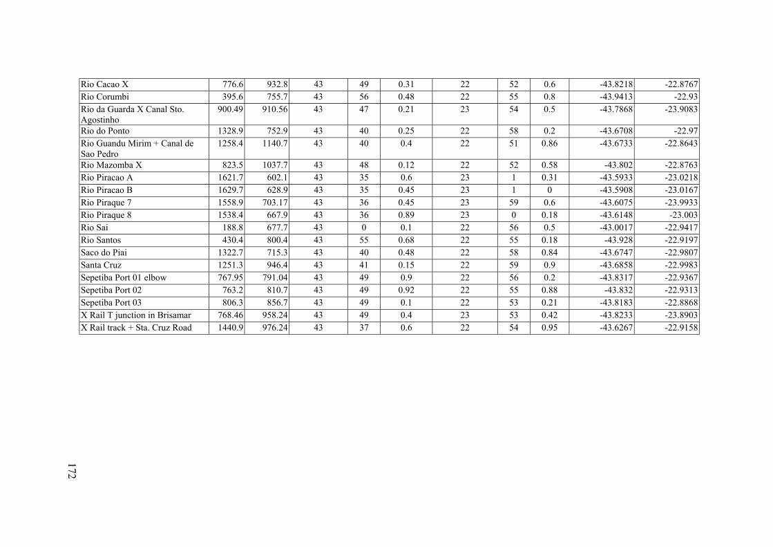
Rio Cacao X 776.6 932.8 0.6 43 49 0.31 22 52 -43.8218 -22.8767 Rio Corumbi 395.6 755.7 43 56 0.48 22 55 0.8 -43.9413 -22.93 Rio da Guarda X Canal Sto. Agostinho

900.49 910.56 43 47 0.21 23 54 0.5 -43.7868 -23.9083

Rio do Ponto 1328.9 752.9 0.25 0.2 43 40 22 58 -43.6708 -22.97 Rio Guandu Mirim + Canal de Sao Pedro

1258.4 0.86 1140.7 43 40 0.4 22 51 -43.6733 -22.8643

Rio Mazomba X 823.5 1037.7 43 48 0.12 22 52 0.58 -43.802 -22.8763 Rio Piracao A 1621.7 602.1 43 35 0.6 23 1 0.31 -43.5933 -23.0218 Rio Piracao B 1629.7 628.9 43 35 0.45 23 1 0 -43.5908 -23.0167 Rio Piraque 7 1558.9 703.17 43 36 0.45 23 59 0.6 -43.6075 -23.9933 Rio Piraque 8 1538.4 667.9 43 36 0.89 23 0 0.18 -43.6148 -23.003 Rio Sai 188.8 677.7 43 0 0.1 22 56 0.5 -43.0017 -22.9417 Rio Santos 430.4 800.4 43 55 0.68 22 55 0.18 -43.928 -22.9197 Saco do Piai 1322.7 715.3 43 40 0.48 22 58 0.84 -43.6747 -22.9807 Santa Cruz 1251.3 946.4 43 41 0.15 22 59 0.9 -43.6858 -22.9983 Sepetiba Port 01 elbow 767.95 791.04 43 49 0.9 22 56 0.2 -43.8317 -22.9367 Sepetiba Port 02 763.2 810.7 43 49 0.92 22 55 0.88 -43.832 -22.9313 Sepetiba Port 03 806.3 856.7 43 49 0.1 22 53 0.21 -43.8183 -22.8868 X Rail T junction in Brisamar 768.46 958.24 43 49 0.4 23 53 0.42 -43.8233 -23.8903 X Rail track + Sta. Cruz Road 1440.9 976.24 43 37 0.6 22 54 0.95 -43.6267 -22.9158



221

172

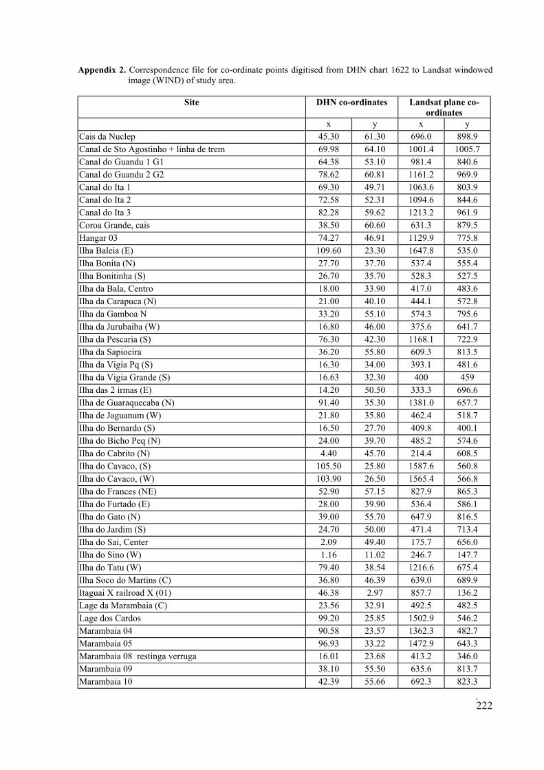
Appendix 2. Correspondence file for co-ordinate points digitised from DHN chart 1622 to Landsat windowed image (WIND) of study area.

GIS AND REMOTE SENSING - BASED MODELS FOR DEVELOPMENT 222

DHN co-ordinates Site Landsat plane co-ordinates

x y x y 45.30 61.30 696.0 898.9

Canal de Sto Agostinho + linha de trem 69.98 64.10 1001.4 1005.7 64.38 53.10 981.4

Canal do Guandu 2 G2 78.62 60.81 1161.2 969.9 69.30 49.71 1063.6

Canal do Ita 2 72.58 52.31 1094.6 844.6 Canal do Ita 3 82.28 59.62 1213.2 961.9 Coroa Grande, cais 38.50 60.60 631.3 879.5 Hangar 03 74.27 46.91 1129.9 775.8 Ilha Baleia (E) 109.60 23.30 1647.8 535.0 Ilha Bonita (N) 27.70 37.70 537.4 555.4 Ilha Bonitinha (S) 26.70 35.70 528.3 527.5 Ilha da Bala, Centro 18.00 33.90 417.0 483.6 Ilha da Carapuca (N) 21.00 40.10 444.1 572.8 Ilha da Gamboa N 33.20 55.10 574.3 795.6 Ilha da Jurubaiba (W) 16.80 46.00 375.6 641.7 Ilha da Pescaria (S) 76.30 42.30 1168.1 722.9 Ilha da Sapioeira 36.20 55.80 609.3 813.5 Ilha da Vigia Pq (S) 16.30 34.00 393.1 481.6 Ilha da Vigia Grande (S) 16.63 32.30 400 459 Ilha das 2 irmas (E) 14.20 50.50 333.3 696.6 Ilha de Guaraquecaba (N) 91.40 35.30 1381.0 657.7 Ilha de Jaguanum (W) 21.80 35.80 462.4 518.7 Ilha do Bernardo (S) 16.50 27.70 409.8 400.1 Ilha do Bicho Peq (N) 24.00 574.6 39.70 485.2 Ilha do Cabrito (N) 4.40 45.70 214.4 608.5 Ilha do Cavaco, (S) 105.50 560.8 25.80 1587.6 Ilha do Cavaco, (W) 103.90 26.50 1565.4 566.8

52.90 57.15 827.9 865.3 Ilha do Furtado (E) 28.00 39.90 536.4 586.1 Ilha do Gato (N) 39.00 55.70 647.9 816.5 Ilha do Jardim (S) 24.70 50.00 471.4 713.4 Ilha do Sai, Center 2.09 49.40 175.7 656.0 Ilha do Sino (W) 1.16 11.02 246.7 147.7 Ilha do Tatu (W) 79.40 38.54 1216.6 675.4 Ilha Soco do Martins (C) 36.80 46.39 639.0 689.9

46.38 2.97 857.7 Lage da Marambaia (C) 23.56 32.91 492.5 482.5 Lage dos Cardos 99.20 25.85 1502.9 546.2 Marambaia 04 90.58

96.93 33.22 1472.9 Marambaia 08 restinga verruga 16.01 23.68 413.2 346.0

38.10 55.50 635.6 Marambaia 10 42.39 55.66 692.3 823.3

Cais da Nuclep

Canal do Guandu 1 G1 840.6

Canal do Ita 1 803.9

Ilha do Frances (NE)

Itaguai X railroad X (01) 136.2

23.57 1362.3 482.7 Marambaia 05 643.3

Marambaia 09 813.7
OF AQUACULTURE AND FISHERIES IN THE COASTAL ZONE:

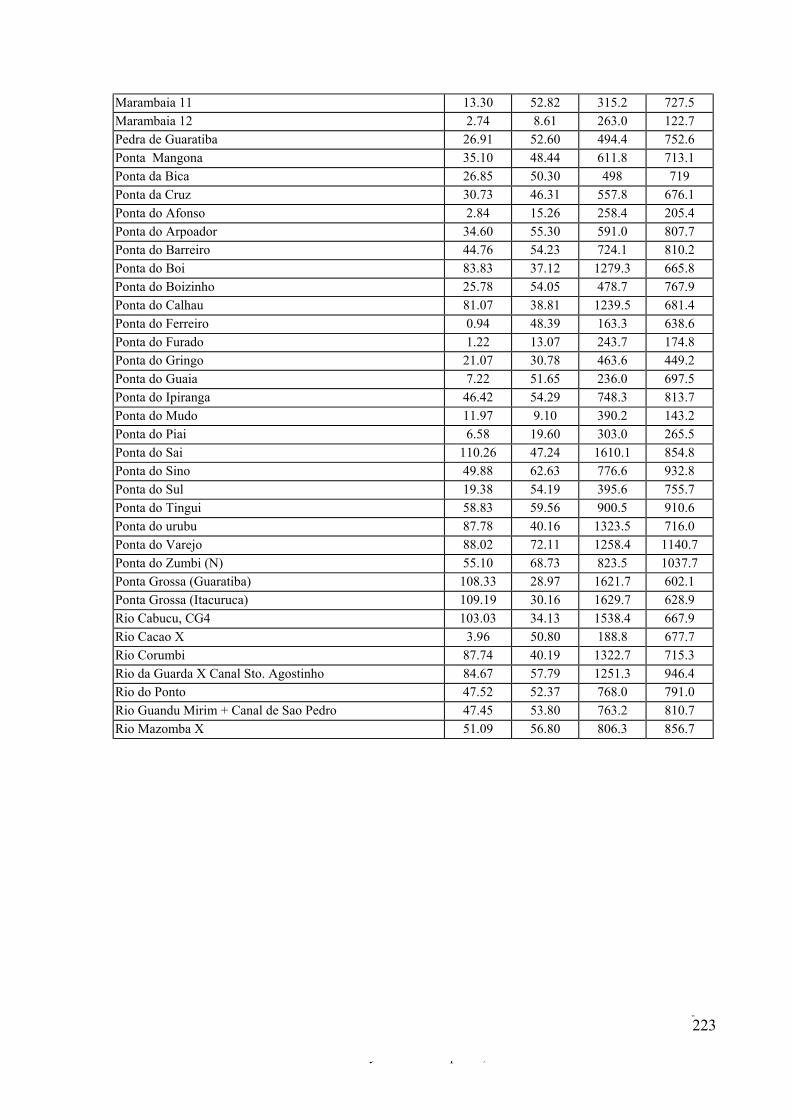
Marambaia 11 727.5 13.30 52.82 315.2 Marambaia 12 2.74 8.61 263.0 122.7

26.91 52.60 494.4 Ponta Mangona 35.10 48.44 611.8 713.1

26.85 50.30 498 Ponta da Cruz 30.73 46.31 557.8 676.1 Ponta do Afonso 2.84 205.4 15.26 258.4 Ponta do Arpoador 34.60 55.30 591.0 807.7

Ponta do Boi 83.83 37.12 1279.3 665.8

Ponta do Calhau 81.07 38.81 1239.5 681.4 Ponta do Ferreiro 0.94 48.39 163.3 638.6

13.07 243.7 Ponta do Gringo 21.07 30.78 463.6 449.2 Ponta do Guaia 7.22 51.65 236.0 697.5 Ponta do Ipiranga 46.42 54.29 748.3 813.7 Ponta do Mudo 11.97 9.10 390.2 143.2 Ponta do Piai 6.58 19.60 303.0 265.5 Ponta do Sai 110.26 47.24 1610.1 854.8

49.88 62.63 776.6 932.8 Ponta do Sul 19.38 54.19 395.6 755.7 Ponta do Tingui 58.83 59.56 900.5 910.6 Ponta do urubu 87.78 40.16 1323.5 716.0 Ponta do Varejo 88.02 72.11 1258.4 1140.7 Ponta do Zumbi (N) 55.10 68.73 823.5 1037.7

108.33 28.97 1621.7 602.1 Ponta Grossa (Itacuruca) 109.19 30.16 1629.7 628.9 Rio Cabucu, CG4 103.03 34.13 1538.4 667.9 Rio Cacao X 3.96 50.80 188.8 677.7 Rio Corumbi 87.74 40.19 1322.7 715.3 Rio da Guarda X Canal Sto. Agostinho 84.67 57.79 1251.3 946.4 Rio do Ponto 47.52 52.37 768.0 791.0 Rio Guandu Mirim + Canal de Sao Pedro 47.45 53.80 763.2 810.7 Rio Mazomba X

Pedra de Guaratiba 752.6

Ponta da Bica 719

Ponta do Barreiro 44.76 54.23 724.1 810.2

Ponta do Boizinho 25.78 54.05 478.7 767.9

Ponta do Furado 1.22 174.8

Ponta do Sino

Ponta Grossa (Guaratiba)

51.09 56.80 806.3 856.7



223

Appendix 3. Drogue tracks, monitored in Sepetiba Bay in 1996.

Date Time Drogue nº: Waypoint Sal ‰ Temp °C Latitude Longitude Depth (m) - 12:20 1 - 31 29 22°56'867 43°52'350 4.3 - 2 - - - - - - - 3 -

- 8:05

4

- 05.03.96

8:19 - 22°59'280 43°55'230

05.03.96 8:28 - - - 22°59'088 43°55'042

05.03.96 8:30 - - - 4 -

05.03.96 - - - - 22°58'968 43°55'290

05.03.96 9:00 - - - 4 - 22°58'957 43°54'968

----------- -

- -

-

05.03.96 - -

- 05.03.96

-

43°53'693

- - - - - - 4 - - - - - -

05.03.96 8:04 1 - - 22°59'255 43°55'95 - 05.03.96 2 - - - 22°59'242 43°55'110 - 05.03.96 8:07 3 - - - 22°59'183 43°55'073 - 05.03.96 8:09 - - - 22°59'138 43°55'063 - 05.03.96 8:13 1 - - - 22°59'265 43°55'177 - 05.03.96 8:13 1 - - 22°59'265 43°55'177 -

8:14 2 - - - 22°59'240 43°55'203 - 05.03.96 8:16 3 - - - 22°59'220 43°55'110 - 05.03.96 4 - - - 22°59'163 43°55'055 05.03.96 8:23 1 - - - -

1 - 22°59'088 43°55'075 - 05.03.96 8:29 2 - - -

3 - 22°59'002 43°54'998 05.03.96 8:31 - - ----------- --------- -

9:03 1 - 22°59'013 43°55'293 05.03.96 9:02 2 - - -

3 - 22°58'972 43°55'145 05.03.96 8:55 - - - 05.03.96 9:10 1 - - - ------------ 05.03.96 9:11 2 - - - 22°58'962 43°55'305 - 05.03.96 9:15 3 - - - 22°59'008 43°55'172 05.03.96 12:37 1 A - 22°56'863 43°52'420 - 05.03.96 12:39 2 B - - 22°56'895 43°52'393 - 05.03.96 12:40 3 C - - 22°56'933 43°52'375 - 05.03.96 12:41 4 D - 22°56'943 43°52'365 - 05.03.96 12:43 1 E - - 22°56'775 43°52'338 -

12:44 2 F - - 22°56'827 43°52'298 05.03.96 12:45 3 G - - 22°56'855 43°52'255 05.03.96 12:46 4 H - 22°56'890 43°52'262 -

14:46 1 - 31 26 22°58'575 43°53'808 18.0 05.03.96 14:47 2 - - - 22°58'542 43°53'812 - 05.03.96 14:48 3 - - - 22°58'502 43°53'815 - 05.03.96 14:49 4 - - - 22°58'470 43°53'812 - 05.03.96 14:52 1 - - 22°58'595 43°53'687 - 05.03.96 14:53 2 - - - 22°58'548 43°53'692 - 05.03.96 14:54 3 - - - 22°58'492 - 05.03.96 14:55 4 - - - 22°58'452 43°53'697 -



224

Date Time Drogue nº: Waypoint Sal ‰ Temp°C Latitude Longitude Depth (m) 16:25 1 - 31 26 22°59'385 43°54'602 4.6

05.03.96 16:27 2 - - - 22°59'638 43°54'638 - 05.03.96 16:29 3 - -

-

4

22°59'638 - -

05.03.96 4 -

- 18:19

- 43°54'968 2

- -

10:42 - --------- 10:42 - - - 22°59'795 -

3 - 22°59'795 - 4 43°55'093

28 06.03.96 -

- 43°56'267'' 14:14 23°00'781'' 14:18 1 23°00'489'' 43°56'207''

06.03.96 2 - 14:21 - - - 14:26 - 43°56'191''

1 23°00'239'' 43°56'726''

23°00'240'' 15:21 - -

-

15:29 - - 23°00'266'' 43°56'831'' - 06.03.96 -

- 22°59'280 43°54'660 - 05.03.96 16:30 4 - - - 22°59'207 43°54'745 - 05.03.96 16:35 1 - - - 22°59'398 43°54'588 05.03.96 16:38 2 - - - 22°59'288 43°54'628 - 05.03.96 16:40 3 - - - 22°59'268 43°54'657 - 05.03.96 16:42 - - - 22°59'220 43°54'952 - 05.03.96 17:59 1 - - - 22°59'385 43°54'602 - 05.03.96 18:00 2 - - - 43°54'638 - 05.03.96 18:02 3 - - 22°59'280 43°54'660

18:04 - - 22°59'207 43°54'745 - 05.03.96 18:10 1 - - - 22°59'398 43°54'588 - 05.03.96 18:13 2 - - - 22°59'288 43°54'628 - 05.03.96 18:14 3 - - 22°59'268 43°54'657 - 05.03.96 4 - - - 22°59'220 43°54'952 - 06.03.96 10:07 1 - - 22°58'957 - 06.03.96 10:09 - - - 22°59'682 43°54'897 - 06.03.96 10:10 3 - - 22°59'737 43°54'882 - 06.03.96 10:12 4 - - 22°59'813 43°54'813 - 06.03.96 1 - - ----------- - 06.03.96 2 43°54'808 06.03.96 10:51 - - 43°54'808

------- - - - 22°59'770 - 06.03.96 14:07 1 - 33 23°00'580" 43°56'145'' 14.6

14:09 2 - - 23°00'628" 43°56'200'' - 06.03.96 14:11 3 - - 23°00'679'' - 06.03.96 4 - - - 43°56'319'' - 06.03.96 - - - -

14:19 - - 23°00'503'' 43°56'209'' - 06.03.96 3 - 23°00'591'' 43°56'290'' 06.03.96 4 - - 23°00'612'' - 06.03.96 15:08 - 31 27 43°56'627'' - 06.03.96 15:12 2 - - - 23°00'257'' - 06.03.96 15:14 3 - - - 43°56'836'' - 06.03.96 4 - 23°00'094'' 43°56'738'' - 06.03.96 15:25 1 - - 23°00'305'' 43°56'664'' - 06.03.96 15:26 2 - - - 23°00'297'' 43°56'715'' - 06.03.96 3 -

15:31 4 - - 23°00'114'' 43°56'647''

05.03.96



225

Date Time Drogue nº: Waypoint Sal ‰ Temp°C Latitude Depth (m) Longitude 06.03.96 16:33 1 - - 31 23°01'231'' 43°56'822'' - 06.03.96 16:35 2

16:37 - - - 43°56'945'' -

06.03.96 16:45 - 23°01'276'' - - 23°01'229'' 43°56'994'' -

16:41 - - 43°57'326''

16:47 - 16:49 - 23°01'131'' 43°57'233'' - 10:24 1 25 22°57'334'' 43°51'784'' 10:26 - 22°57'455'' 43°51'820'' 10:27 10:28 -

-

- - 43°52'014'' -

3 - - 43°52'023'' - 2 - - 43°52'045''

07.03.96 - 4 - - 43°51'928''

07.03.96 10:51 1 25 - - 10:52 22°57'143'' 43°51'925''

- 22°57'106'' 10:54 11:07 1 - 22°57'234'' 43°51'971'' -

07.03.96 11:09 2 - - - 22°57'221'' 43°51'913''

- 22°56'814''

- 4

07.03.96 - 22°56'836''

- - 07.03.96 22°56'774''

- - - 23°01'155'' 43°56'854'' - 06.03.96 3 - - 23°01'070'' 43°56'889'' - 06.03.96 16:39 4 - 23°00'959''

1 - - 43°56'952'' - 06.03.96 16:43 2 - 06.03.96 3 - - 23°01'112'' 43°57'001'' 06.03.96 16:52 4 - - - 23°01'970'' - 06.03.96 2 - - - 23°01'232'' 43°57'055'' 06.03.96 3 - - 07.03.96 - 29 16.8 07.03.96 2 - - - 07.03.96 3 - - - 22°57'519'' 43°51'845'' - 07.03.96 4 - - 22°57'566'' 43°51'878'' - 07.03.96 10:33 1 - - 22°57'332'' 43°51'884'' - 07.03.96 10:35 2 - - - 22°57'422'' 43°51'926'' - 07.03.96 10:37 3 - - - 22°57'497'' 43°51'967'' 07.03.96 10:40 4 - - 22°57'564'' 07.03.96 10:42 - 22°57'485'' 07.03.96 10:46 - 22°57'394'' -

10:48 1 - - 22°57'326'' 43°51'986'' - 07.03.96 ------ - 22°57'524'' -

- 22°57'175'' 43°51'977'' 07.03.96 2 - - - - 07.03.96 10:53 3 - - 43°51'855'' - 07.03.96 4 - - - 22°57'082'' 43°51'786'' - 07.03.96 - -

- 07.03.96 11:11 3 - - - 22°57'164'' 43°51'829'' - 07.03.96 11:13 4 - - - 22°57'081'' 43°51'716'' - 07.03.96 11:31 1 - - - 22°56'859'' 43°51'835'' 07.03.96 11:29 2 - - - 43°51'888'' - 07.03.96 11:33 3 - - 22°56'779'' 43°51'941'' - 07.03.96 11:35 - - - 22°56'741'' 43°52'016'' -

11:40 1 - - - 22°56'905'' 43°51'849'' 07.03.96 11:42 2 - - - 43°51'871'' - 07.03.96 11:43 3 - - 22°56'787'' 43°51'865''

11:45 4 - - - 43°51'984'' - 07.03.96 11:46 2 - - - 22°56'800'' 43°51'058'' - 07.03.96 11:47 1 - - - 22°56'848'' 43°52'213'' - 07.03.96 11:48 4 - - - 22°56'873'' 43°52'271'' -



226

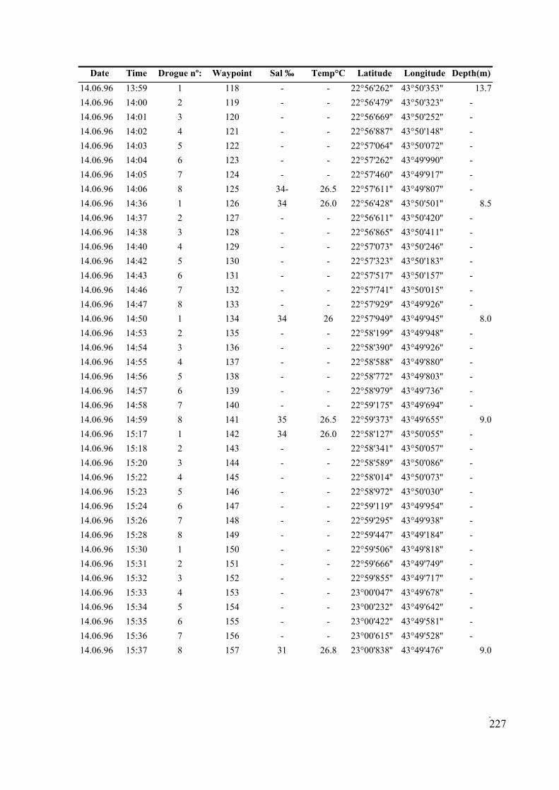
Date Time Drogue nº: Waypoint Sal ‰ Temp°C Latitude Longitude Depth(m) 14.06.96 13:59 1 118 - - 22°56'262'' 43°50'353'' 13.7 14.06.96 14:00 2 119 - - 22°56'479'' 43°50'323'' - 14.06.96 14:01 43°50'252'' 14.06.96

124 34-

5 43°50'183'' 14.06.96 14:43 6

7 14.06.96 - 14.06.96

14.06.96 -

14.06.96 22°59'373''

14.06.96

14.06.96 43°50'073''

-

7

3 120 - - 22°56'669'' - 14:02 4 121 - - 22°56'887'' 43°50'148'' -

14.06.96 14:03 5 122 - - 22°57'064'' 43°50'072'' - 14.06.96 14:04 6 123 - - 22°57'262'' 43°49'990'' - 14.06.96 14:05 7 - - 22°57'460'' 43°49'917'' - 14.06.96 14:06 8 125 26.5 22°57'611'' 43°49'807'' - 14.06.96 14:36 1 126 34 26.0 22°56'428'' 43°50'501'' 8.5 14.06.96 14:37 2 127 - - 22°56'611'' 43°50'420'' - 14.06.96 14:38 3 128 - - 22°56'865'' 43°50'411'' - 14.06.96 14:40 4 129 - - 22°57'073'' 43°50'246'' - 14.06.96 14:42 130 - - 22°57'323'' -

131 - - 22°57'517'' 43°50'157'' - 14.06.96 14:46 132 - - 22°57'741'' 43°50'015'' -

14:47 8 133 - 22°57'929'' 43°49'926'' - 14:50 1 134 34 26 22°57'949'' 43°49'945'' 8.0

14.06.96 14:53 2 135 - - 22°58'199'' 43°49'948'' - 14:54 3 136 - - 22°58'390'' 43°49'926''

14.06.96 14:55 4 137 - - 22°58'588'' 43°49'880'' - 14.06.96 14:56 5 138 - - 22°58'772'' 43°49'803'' - 14.06.96 14:57 6 139 - - 22°58'979'' 43°49'736'' -

14:58 7 140 - - 22°59'175'' 43°49'694'' - 14.06.96 14:59 8 141 35 26.5 43°49'655'' 9.0

15:17 1 142 34 26.0 22°58'127'' 43°50'055'' - 14.06.96 15:18 2 143 - - 22°58'341'' 43°50'057'' -

15:20 3 144 - - 22°58'589'' 43°50'086'' - 14.06.96 15:22 4 145 - - 22°58'014'' - 14.06.96 15:23 5 146 - 22°58'972'' 43°50'030'' - 14.06.96 15:24 6 147 - - 22°59'119'' 43°49'954'' - 14.06.96 15:26 148 - - 22°59'295'' 43°49'938'' - 14.06.96 15:28 8 149 - - 22°59'447'' 43°49'184'' - 14.06.96 15:30 1 150 - - 22°59'506'' 43°49'818'' - 14.06.96 15:31 2 151 - - 22°59'666'' 43°49'749'' - 14.06.96 15:32 3 152 - - 22°59'855'' 43°49'717'' - 14.06.96 15:33 4 153 - - 23°00'047'' 43°49'678'' - 14.06.96 15:34 5 154 - - 23°00'232'' 43°49'642'' - 14.06.96 15:35 6 155 - - 23°00'422'' 43°49'581'' - 14.06.96 15:36 7 156 - - 23°00'615'' 43°49'528'' - 14.06.96 15:37 8 157 31 26.8 23°00'838'' 43°49'476'' 9.0



227

Date Time Drogue nº: Waypoint Sal ‰ Temp°C Latitude Longitude Depth (m) 14.06.96 15:55 1 158 22°59'528'' 43°50'097'' 14.06.96 15:56 2 159 22°59'694'' 43°49'978'' 14.06.96 15:58 3 160 22°59'953'' 43°49'990'' 14.06.96 15:59 4 161 23°00'127'' 43°49'883''

16:02

8 43°53'952''

14.06.96 2 22°57'634'' 3

14:49 43°54'064'' 14.06.96 5

14:55

22°58'302''

7 26

26 3

16:27 5 22°55'985''

14.06.96 31

14.06.96 16:00 5 162 23°00'353'' 43°49'889'' 14.06.96 16:01 6 163 23°00'507'' 43°49'791'' 14.06.96 7 164 23°00'689'' 43°49'741'' 14.06.96 16:03 165 23°00'944'' 43°49'723'' 14.06.96 14:45 1 1 22°57'539''

14:47 2 43°53'998'' 14.06.96 14:48 3 22°57'727'' 43°54'029'' 14.06.96 4 4 22°57'832''

14:50 5 22°57'951'' 43°54'103'' 14.06.96 14:54 6 6 22°58'017'' 43°54'163'' 14.06.96 7 7 22°58'151'' 43°54'197'' 14.06.96 14:56 8 8 43°54'268'' 14.06.96 15:13 1 9 22°57'551'' 43°54'002'' 14.06.96 15:14 2 10 22°57'539'' 43°54'249'' 14.06.96 15:15 3 11 22°57'581'' 43°54'317'' 14.06.96 15:16 4 12 22°57'595'' 43°54'374'' 14.06.96 15:18 5 13 22°57'674'' 43°54'442'' 14.06.96 15:19 6 14 22°57'775'' 43°54'493'' 14.06.96 15:20 7 15 22°57'872'' 43°54'479'' 14.06.96 15:21 8 16 22°57'979'' 43°54'587'' 14.06.96 15:44 1 17 16 29 22°55'599'' 43°48'844'' 14.06.96 15:45 2 18 22°55'707'' 43°48'878'' 14.06.96 15:46 3 19 22°55'799'' 43°48'897'' 14.06.96 15:47 4 20 7 28 22°55'899'' 43°48'905'' 14.06.96 15:48 5 21 22°56'017'' 43°48'923'' 14.06.96 15:49 6 22 22°56'105'' 43°48'953'' 14.06.96 15:50 23 22°56'224'' 43°48'985'' 14.06.96 15:51 8 24 28 22°56'360'' 43°49'024'' 14.06.96 16:14 1 25 22°55'345'' 43°49'098'' 14.06.96 16:23 2 22°55'541'' 43°49'341'' 14.06.96 16:24 27 22°55'660'' 43°49'489'' 14.06.96 16:26 4 28 22°55'846'' 43°49'581'' 14.06.96 29 43°49'617''

16:29 6 30 22°56'112'' 43°49'667'' 14.06.96 16:31 7 22°56'263'' 43°49'681'' 14.06.96 16:31 8 32 22°56'405'' 43°49'718'' 14.06.96 16:57 1 34 22°56'271'' 43°47'791''



228

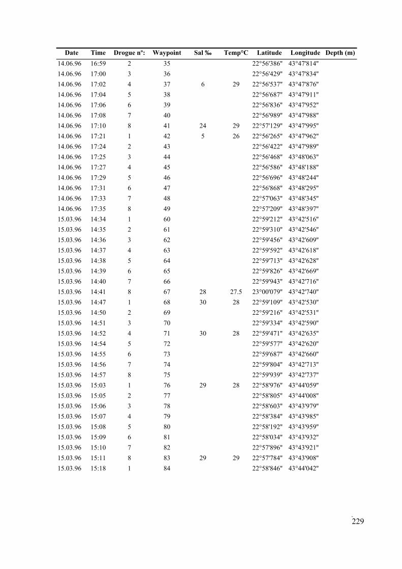
Date Time Drogue nº: Waypoint Sal ‰ Temp°C Latitude Longitude Depth (m) 14.06.96 16:59 2 35 22°56'386'' 43°47'814'' 14.06.96 17:00

37

40 17:10 29

42 43°47'962'' 14.06.96 17:24

14.06.96 22°57'063''

14.06.96 1 22°59'212''

15.03.96 3 22°59'456''

15.03.96 5 22°59'713''

15.03.96 14:39 7

14:41 28 27.5 1 68 22°59'109'' 43°42'530''

3 70 43°42'590'' 4 71 22°59'471''

6 73

15.03.96 43°42'713''

15:03 1

15.03.96 43°43'985''

3 36 22°56'429'' 43°47'834'' 14.06.96 17:02 4 6 29 22°56'537'' 43°47'876'' 14.06.96 17:04 5 38 22°56'687'' 43°47'911'' 14.06.96 17:06 6 39 22°56'836'' 43°47'952'' 14.06.96 17:08 7 22°56'989'' 43°47'988'' 14.06.96 8 41 24 22°57'129'' 43°47'995'' 14.06.96 17:21 1 5 26 22°56'265''

2 43 22°56'422'' 43°47'989'' 14.06.96 17:25 3 44 22°56'468'' 43°48'063'' 14.06.96 17:27 4 45 22°56'586'' 43°48'188'' 14.06.96 17:29 5 46 22°56'696'' 43°48'244''

17:31 6 47 22°56'868'' 43°48'295'' 14.06.96 17:33 7 48 43°48'345''

17:35 8 49 22°57'209'' 43°48'397'' 15.03.96 14:34 60 43°42'516''

14:35 2 61 22°59'310'' 43°42'546'' 15.03.96 14:36 62 43°42'609''

14:37 4 63 22°59'592'' 43°42'618'' 15.03.96 14:38 64 43°42'628''

6 65 22°59'826'' 43°42'669'' 15.03.96 14:40 66 22°59'943'' 43°42'716'' 15.03.96 8 67 23°00'079'' 43°42'740'' 15.03.96 14:47 30 28 15.03.96 14:50 2 69 22°59'216'' 43°42'531'' 15.03.96 14:51 22°59'334'' 15.03.96 14:52 30 28 43°42'635'' 15.03.96 14:54 5 72 22°59'577'' 43°42'620'' 15.03.96 14:55 22°59'687'' 43°42'660''

14:56 7 74 22°59'804'' 15.03.96 14:57 8 75 22°59'939'' 43°42'737'' 15.03.96 76 29 28 22°58'976'' 43°44'059'' 15.03.96 15:05 2 77 22°58'805'' 43°44'008'' 15.03.96 15:06 3 78 22°58'603'' 43°43'979''

15:07 4 79 22°58'384'' 15.03.96 15:08 5 80 22°58'192'' 43°43'959'' 15.03.96 15:09 6 81 22°58'034'' 43°43'932'' 15.03.96 15:10 7 82 22°57'896'' 43°43'921'' 15.03.96 15:11 8 83 29 29 22°57'784'' 43°43'908'' 15.03.96 15:18 1 84 22°58'846'' 43°44'042''



229

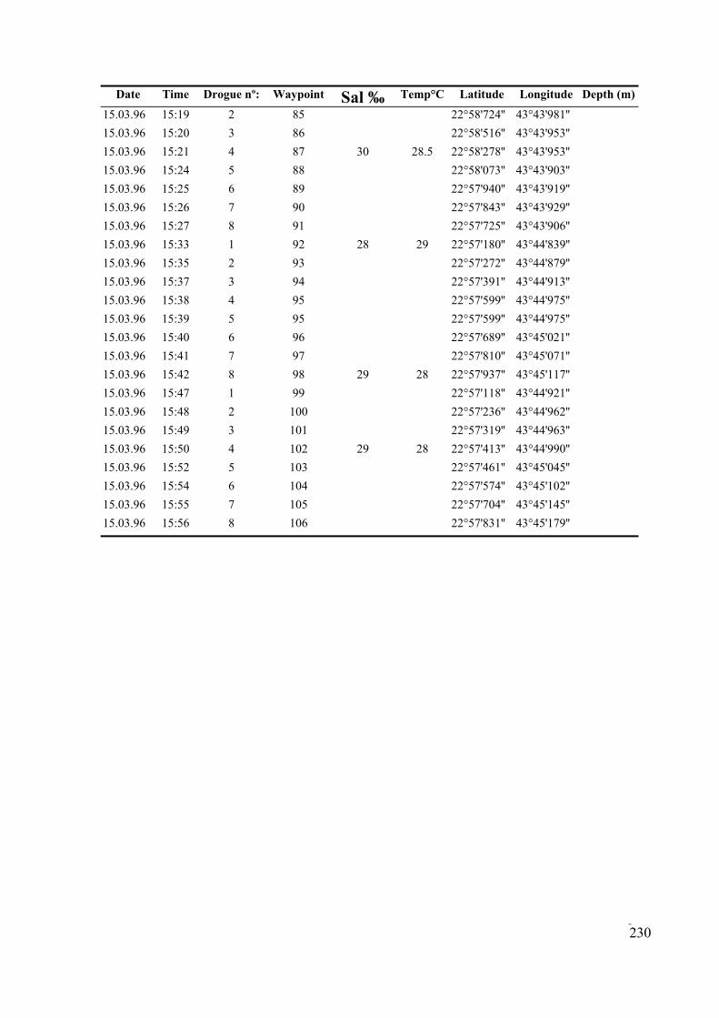
Date Longitude Time Drogue nº: Waypoint Sal ‰ Temp°C Latitude Depth (m)

15.03.96 15:19 2 85 22°58'724'' 43°43'981'' 15.03.96 15:20 3 86 22°58'516'' 43°43'953''

22°57'940''

43°43'906'' 28

22°57'599'' 96

15:41 7 22°57'810'' 15.03.96

15:47 1 22°57'118'' 15.03.96 100 43°44'962''

15.03.96 102 29

15:52 5 22°57'461'' 15.03.96 104 43°45'102''

15:55 7 15:56 106

15.03.96 15:21 4 87 30 28.5 22°58'278'' 43°43'953'' 15.03.96 15:24 5 88 22°58'073'' 43°43'903'' 15.03.96 15:25 6 89 43°43'919'' 15.03.96 15:26 7 90 22°57'843'' 43°43'929'' 15.03.96 15:27 8 91 22°57'725'' 15.03.96 15:33 1 92 29 22°57'180'' 43°44'839'' 15.03.96 15:35 2 93 22°57'272'' 43°44'879'' 15.03.96 15:37 3 94 22°57'391'' 43°44'913'' 15.03.96 15:38 4 95 22°57'599'' 43°44'975'' 15.03.96 15:39 5 95 43°44'975'' 15.03.96 15:40 6 22°57'689'' 43°45'021'' 15.03.96 97 43°45'071''

15:42 8 98 29 28 22°57'937'' 43°45'117'' 15.03.96 99 43°44'921''

15:48 2 22°57'236'' 15.03.96 15:49 3 101 22°57'319'' 43°44'963''

15:50 4 28 22°57'413'' 43°44'990'' 15.03.96 103 43°45'045''

15:54 6 22°57'574'' 15.03.96 105 22°57'704'' 43°45'145'' 15.03.96 8 22°57'831'' 43°45'179''



230

Appendix 4 Surface salinity, temperature and depth values at different sites in Sepetiba bay.

Date

Time latitude longitude surface salinity

S ‰

Surface Temperature

°C

Depth

m 15.1.97 - 22.55.307 43.52.839 30 27 6.7 15.1.97 - 22.54.653 43.51.086 28 29 2.1 15.1.97 - 22.54.577 43.50.895 29 28 1.2 15.1.97 - 22.55.616 43.51.083 31 26.5 4.3 15.1.97 - 22.55.076 43.50.639 22 27 4.9 15.1.97 - 22.56.157 43.49.906 10 29 9.4 15.1.97 11:03 22.55.436 43.48.938 14 29.5 1.2 15.1.97 - 22.55.261 43.48.727 20 29.5 0.6 15.1.97 - 15.1.97 29

15.1.97

15.1.97

15.1.97

15.1.97

15.1.97

15.1.97

15.1.97

15.1.97 15.1.97 31 6.4 15.1.97 - 22.55.680

22.56.044 43.48.628 11 30 4.3 - 22.56.125 43.48.081 2 1.5

15.1.97 11:34 22.56.878 43.56.878 5 31 0.0 15.1.97 - 22.57.651 43.48.529 3 29.5 6.4

- 22.57.651 43.48.529 26 29 6.4 15.1.97 - 22.59.493 43.50.034 28 29 7.9 15.1.97 - 23.01.318 43.50.292 30 29 8.8

- 23.02.959 43.51.046 29 29 0.3 15.1.97 13:09 23.01.324 43.53.350 31 28.5 4.6 15.1.97 - 23.01.759 43.54.089 31 30 1.2

- 23.02.448 43.53.993 31 28 2.4 15.1.97 - 23.00.792 43.55.551 35 25 7.6 15.1.97 - 23.00.201 43.55.084 33 27 10.4

13:54 23.01.341 43.57.256 34 27 7.3 15.1.97 - 23.00.279 43.57.322 33 27 9.1 15.1.97 14:40 23.00.097 43.56.474 35 25 7.9

- 22.59.283 43.55.723 35 24 20.4 15.1.97 - 22.59.250 43.54.901 31 28 9.8 15.1.97 - 22.59.745 43.54.630 33 26.5 14.0

- 22.59.060 43.54.209 30 29 10.1 15.1.97 - 22.58.632 43.54.766 34 25 24.4 15.1.97 - 22.58.297 43.55.188 33 26 21.9

15:15 22.57.831 43.54.466 34 27 25.9 15.1.97 - 22.58.058 43.53.339 30 29 15.8 15.1.97 - 22.57.477 43.52.690 30 28 20.1

- 22.56.624 43.51.721 31 28 18.3 - 22.55.753 43.52.019 27.5

43.51.641 30 26.5 5.5 15.1.97 15:37 22.55.650 43.51.383 31 27 5.5 15.1.97 - 22.55.846 43.50.642 29 28 5.2



231

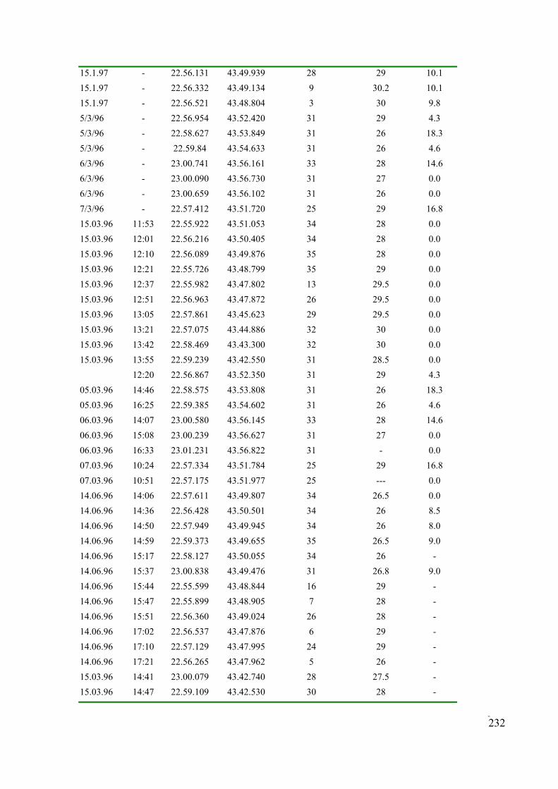
15.1.97 - 22.56.131 43.49.939 28 29 10.1 15.1.97 - 22.56.332 43.49.134 9 30.2 10.1 15.1.97 - 22.56.521 43.48.804 3 30 9.8 5/3/96 - 22.56.954 43.52.420 31

31

- - 31 0.0 - 43.51.720 29 16.8

15.03.96 22.55.922 0.0 12:01 22.56.216 34

15.03.96 28 29

22.55.982 0.0 43.47.872 43.45.623

32 13:42 22.58.469 0.0

22.59.239 31 0.0 43.52.350 29

05.03.96 14:46 31 16:25 26

23.00.580 14.6

16:33 22.57.334

10:51 43.51.977 34

43.49.945 26 14:59 22.59.373 43.49.655 35 26.5 9.0 15:17

15:44 16 14.06.96 43.48.905

22.56.360 43.47.876 29

17:21 43.47.962 5 26 - 14:41 28

43.42.530 28 -

29 4.3 5/3/96 - 22.58.627 43.53.849 26 18.3 5/3/96 - 22.59.84 43.54.633 31 26 4.6 6/3/96 - 23.00.741 43.56.161 33 28 14.6 6/3/96 23.00.090 43.56.730 31 27 0.0 6/3/96 23.00.659 43.56.102 26 7/3/96 22.57.412 25

11:53 43.51.053 34 28 15.03.96 43.50.405 28 0.0

12:10 22.56.089 43.49.876 35 0.0 15.03.96 12:21 22.55.726 43.48.799 35 0.0 15.03.96 12:37 43.47.802 13 29.5 15.03.96 12:51 22.56.963 26 29.5 0.0 15.03.96 13:05 22.57.861 29 29.5 0.0 15.03.96 13:21 22.57.075 43.44.886 30 0.0 15.03.96 43.43.300 32 30 15.03.96 13:55 43.42.550 28.5

12:20 22.56.867 31 4.3 22.58.575 43.53.808 26 18.3

05.03.96 22.59.385 43.54.602 31 4.6 06.03.96 14:07 43.56.145 33 28 06.03.96 15:08 23.00.239 43.56.627 31 27 0.0 06.03.96 23.01.231 43.56.822 31 - 0.0 07.03.96 10:24 43.51.784 25 29 16.8 07.03.96 22.57.175 25 --- 0.0 14.06.96 14:06 22.57.611 43.49.807 26.5 0.0 14.06.96 14:36 22.56.428 43.50.501 34 26 8.5 14.06.96 14:50 22.57.949 34 8.0 14.06.96 14.06.96 22.58.127 43.50.055 34 26 - 14.06.96 15:37 23.00.838 43.49.476

29

17:02 43.47.995



232

31 26.8 9.0 14.06.96 22.55.599 43.48.844 -

15:47 22.55.899 7 28 - 14.06.96 15:51 43.49.024 26 28 - 14.06.96 22.56.537 6 - 14.06.96 17:10 22.57.129 24 29 - 14.06.96 22.56.265 15.03.96 23.00.079 43.42.740 27.5 - 15.03.96 14:47 22.59.109 30

15.03.96 14:52 43.42.635 - 22.59.471 30 28 15.03.96 15:03 29 28 - 15.03.96 15:11 22.57.784 29 - 15.03.96 15:21 22.58.278 43.43.953 30 28.5 15.03.96 22.57.180 43.44.839 29

22.57.937 28 22.57.413 29 -

30.01.97 15.2 33 - 30.01.97 16.1 23.01.700 43.37.399 35 29 - 30.01.97 23.01.611 43.37.682 34 - 30.01.97 23.01.225 43.37.585 34 29.5 30.01.97 17.2 23.01.577 34 29 - 30.01.97 17.2 23.01.151 43.37.637 34 - 31.01.97 10.2 22.59.825 43.55.209 14 31 31.01.97 10.4 23.00.329 10 33 -

22.58.976 43.43.908

- 15:33 28 -

15.03.96 15:42 43.45.117 29 - 15.03.96 15:50 43.44.990 28

23.01.639 43.37.013

16.5 25.5 -

- 43.54.591

43.44.059 29

30

16.5 43.37.798

29.5



233

Appendix 5. Heavy metal content of sediments in Sepetiba Bay. Capes/BC samples were analysed at Institute of Aquaculture, Stirling University. All other samples were analysed by CPRM - Rio de Janeiro.

Date Waypoint Co-ordinates METAL CONTENT IN SEDIMENTS (PPM) Field Trip ID Sample number

latitude longitude Cu Pb Zn Ag Co Ni Cr Cd Fe Mo VCapes/BC 30.0 .98 - 32 29 894 - 8 22°56'21'' 43°47'58'' S1 - - 87 11 - -Capes/BCCapes/BC

43°48'00'' S2 44 87 - - - - -

Capes/BC - S4 100 -

- S9 18

97 1 2 81 1 24

8 40

22 12

30.08.98 - 22°57'54'' 32 578 107

- - - 22 - 413135

- 30.08.98 30.08.98

- 22°57'47''22°58'34''

43°48'58''43°50'00''

S3 83 1.015

- 5 2788 - - 102 9 - 328 - -

30.08.98 - NA NA S5 77 1.3 460 280

- - 53 5 - 408 - -- NA NA S6 0 2.1 - - 65 4 - 465 -

Capes/BC

30.08.98 22°58'48'' 43°46'24'' 18 1.1 1450 - -

-

- 406 - -A 30.01.97 43.41.919 1 4 4 110 N(0.2) 1 8 0.4 42 N(2) 8A 30.01.97 43 10 18 160 N(0.2) 7 9 34 14

Mn450 -

-

Capes/BCCapes/BC

- 30.08.98 -

- 20223.01.90923.01.128

0.843.36.980 2.65 800 N(2) 32

A 30.01.97 73 23.01.484 43.38.008 3 16 24 660 N(0.2) 8 12 52 5.6 3.2 700 N(2) 36A 30.01.97 44 23.01.700 43.37.399 4 14 420 N(0.2) 8 12 50 3.4 2.9 480 L(2) 32A 30.01.97 128 23.01.854 43.54.927 5 3 6 152

345 N(0.2) 2 2

0 10 1.4 0.74 285 N(2) 8

A 30.01.97 23.01.931 43.39.366 6 9 16 N(0.2) 6 38 1.2 2.8 335 L(2) 28A 30.01.97 104 23.02.557 43.43.047 7 8 14 550 N(0.2) 5 8 30 6.4 1.9 215 N(2) 20

A 30.01.97 131 22.57.302 43.54.877 9 7 12 325 N(0.2) 5 7 30 12 2.05 300 N(2)A 30.01.97 113 23.00.329 43.54.591 10 3 4 154

N(0.2) 2 3 14 2.4 0.84 112 L(2) 12

A 30.01.97 130 23.00.048 43.57.005 11 3 6 94500

N(0.2) 1 2 10 0.61.8

0.45 78 N(2)L(2)

816 A 30.01.97 106 22.59.825 43.55.209 14 8 14 N(0.2)

N(0.2)5 8 32 2.4 200

B 13.02.96 JVAJVA

22.54.800 43.50.600 - 23 16 210 410

2 N(1)

6 0.2 1.72 126 N(2)B 13.02.96 22.54.600 43.52.700 - 13 18 N(0.2)

N(0.2) 8 9 38 1.4 2.75 240 L(2) 40

B 13.02.96 JVA 22.55.800 43.55.100 - 9 10 82 8 10 44 0.2 2.45 260 L(2)C 05.03.96 * 22.56.954 43.52.420 1 13 22 720 N(0.2) 6 11

2 55 2.8 3.65 250 N(2) 36

C 05.03.96 * 22.58.627 43.53.849 2 3 10 205 116

N(0.2) 2 16 14

0.4 1.02 100 N(2) 12C 05.03.96 * 22.59.384 43.54.633 3 3 8 N(0.2) 1 1 0.6

1.2 0.82 82 N(2) 8

C 06.03.96 * 23.00.741 43.56.161 4 4 10 148 N(0.2) 3 3 1

1.24 138 N(2) 16 CC

06.03.96 * 23.00.090 43.56.730 5 2 4 80 N(0.2) 2 9 0.6 0.4 42 N(2) 8 06.03.96 * 23.00.659 43.56.102 6 5 8 200 N(0.2) 1 1 14 0.8 0.72 300 N(2)

24



234

185

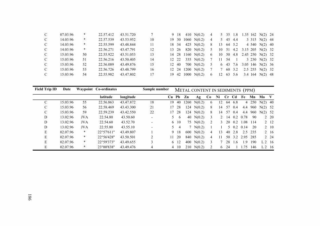
C

07.03.96 * 22.57.412 43.51.720 7 9 18 410 N(0.2) 4 5 35 1.8 1.35

162 N(2) 24C 14.03.96 * 22.57.539 43.53.952 10 19 30 1060 N(0.2) 4 5 45 4.4 3 315 N(2) 44C 14.03.96 * 22.55.599 43.48.844 11 18 34 425 N(0.2) 8 13 64 5.2 4 540 N(2) 40 C 14.03.96 * 22.56.271 43.47.791 12 13 26 820 N(0.2) 5 10 51 4.2 3.15 205 N(2) 32C 15.03.96 50 22.55.922 43.51.053 13 14 28 1160 N(0.2) 6 10 50 4.8 2.45

250 N(2) 32

C 15.03.96 5152

22.56.216 43.50.405 14 12 22 335 N(0.2) 7 11

54 1 3 230 N(2) 32C 15.03.96 22.56.089 43.49.876 15 12 40 700 N(0.2) 5 6 43 7.6

3.05

3.2 146 N(2) 36

C 15.03.96 53 22.56.726 43.48.799 16 12 24 1200 N(0.2) 7 7 60 2.5 255

N(2) 32C 15.03.96 54 22.55.982 43.47.802 17 19 42 1000 N(0.2) 6 12 63 5.6 3.4 164 N(2) 48

Field Trip ID Date Waypoint Co-ordinates Sample number METAL CONTENT IN SEDIMENTS (PPM)

longitude Cu Pb Zn Ag Co Ni Cd Fe Mo VC 5 18 0 2 40 15.03.96 5 22.56.863 43.47.872 19 40 126 N(0.2) 6 1 64 6.8 4 250 N(2)C 15.03.96 56 22.58.469 43.43.300 21 17

17 28 124 N(0.2)

N(0.2) 8 14 57

57 0.4 4.4 960

960 N(2) 52

C 15.03.96 59 22.59.239 43.42.550

22 28 124 40

8 14

0.4 4.4 N(2)

52 D

13.02.96 JVA 22.54.80 43.50.60 - 5 6 N(0.2) 3 2 14 0.2 0.78 90 2 20D 13.02.96 JVA 22.54.60 43.52.70 - 6 10 75

N(0.2) 2 3 20 0.2 1.08 114 2 12

D 13.02.96 JVA 22.55.80 43.55.10 - 5 4 7 N(0.2) 1 1 5 0.2 0.14 20 2 10E 02.07.96 * 22°57'611'' 43.49.807 1 9 18 600 N(0.2) 4 13 40 2.8 2.5 235 2 16E 02.07.96 * 22°56'428'' 43.50.501 2 11 20 840 N(0.2) 4 11 50 3.2 2.95 285 2 24E 02.07.96 * 22°59'373'' 43.49.655 3 6 12 400 N(0.2) 3 7 28 1.6 1.9 190 L 2 16 E 02.07.96 * 23°00'838'' 43.49.476 4 4 10 210 N(0.2) 2 6 24 1 1.75 146 L 2 16

latitude Cr Mn



235

186

Appendix 6. List of sites visited in the Sepetiba bay catchment area and notes as to type of land cover for ground truthing part of GIS study.

Date Position Site ID Description

longitude latitude

10.01.97 43.54.438 22.55.658 Itacuruçá 1 Sandy beach, in Itacuruçá, front of Universidade Federal do Rio de Janeiro lab. Buildings with concrete/asbestos roofing. Urban area, red tiled roofs, cobblestone road 10 m wide and sandy beach just after. Reflective.

10.01.97 43.54.430 22.55.572 Itacuruçá 2 Tile roofs, concrete, road. Some vegetation between houses.

10.01.97 43.54.405 22.55.326 Itacuruçá 3 Outskirts of Itacurucá, housing less dense, and smaller houses.

10.01.97 43.54.156 22.55.198 Itacuruçá 4 Local plants include marsh types such as Typhas, taboas, Vassouras, lírio do brejo and Cyperaceae, 20m alt., Soil sample number 1 taken. Area adjacent to the sea, probably was cleared and leveled.

10.01.97 43.54.174 22.54.973 Itacuruçá 5 Grassland composed of Capim grodura, capim colonião, Panicum spp, pasto limpo. Grass replanted hillsides for protection againts rainfall erosion, Poor growth, just above main coastal road BR101 between Rio and Santos.

10.01.97 43.53.478 22.54.291 Itacuruçá 6 Recently severely denuded area during 1996 torrential rains. Exposed rocky area. about 40 m altitude, very close to BR101. Same place where all the Macumba offerings are placed to the waterfall deity of afro-brazilian religion.

10.01.97 43.53.461 22.54.240 Itacuruçá 7 Same site as above, 50m altitude. Pyrite, sand and gravel large boulders of gneiss = 60% rock and = 5% water coverage. About 100 m or more of exposed rock in the middle of Atlantic rainforest.

10.01.97 43.51.871 22.54.123 Coroa Grande

8 Downtown Coroa Grande in front of railway line and station. Point represents coverage which includes cobblestone road, rail tracks at about 50% and grass, trees and houses = 50%.

43.49.406 22.53.478 Railroad rossing on tarmac road to Ilha da Madeira, at junction where police station is located. Wide strip of tarmac & railroad. Roadside are several heactares of cleared land with poorly developed grassland cover, with many patches of exposed reddish soil. Waterlogged soils from road side to the mangrove fringe.

10.01.97 43.49.477 Same general area as above, on Ilha da Madeira proper. Flat vegetation cleared areas, with exposed rusty coloured soils and poorly developed grassland just on the inside of the Port of Sepetiba entrance gates.

22.54.179 10

10.01.97 9



236

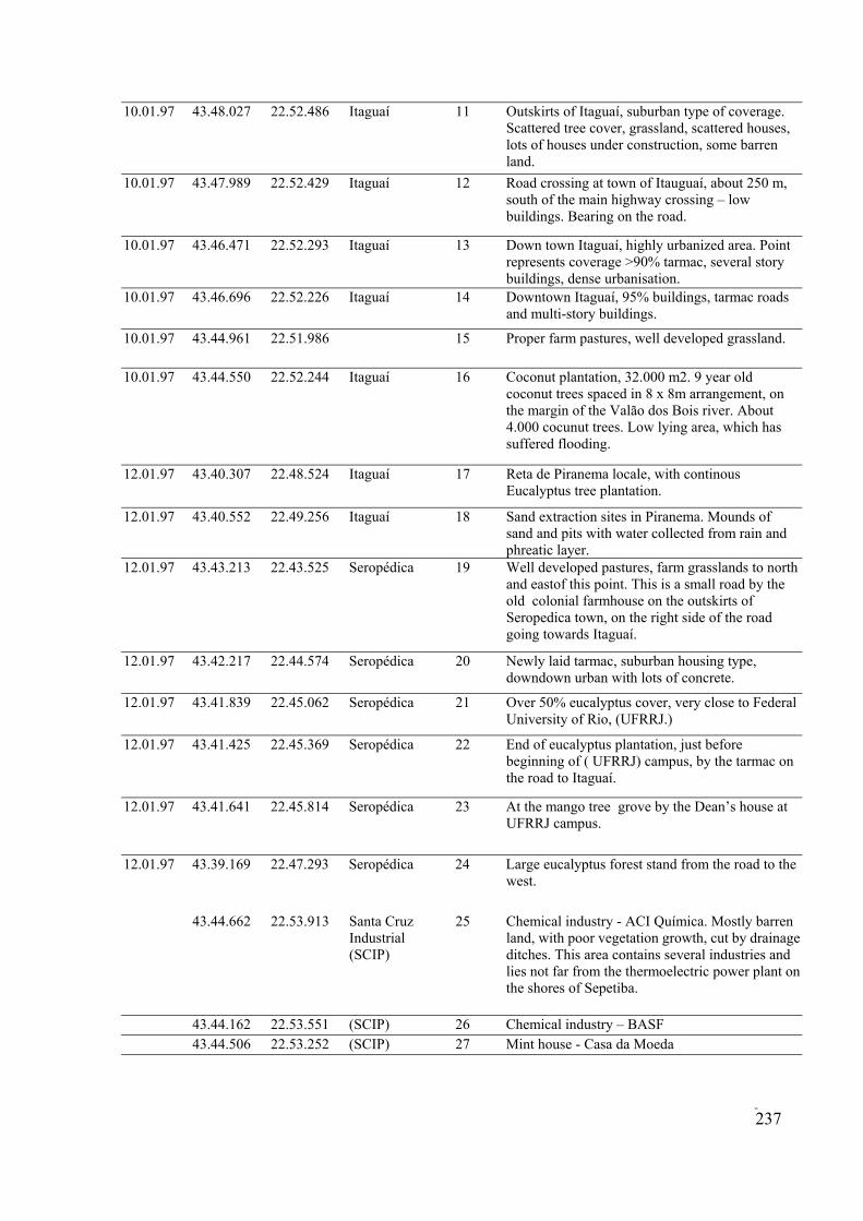
10.01.97 43.48.027 22.52.486 Itaguaí 11 Outskirts of Itaguaí, suburban type of coverage. Scattered tree cover, grassland, scattered houses, lots of houses under construction, some barren land.

43.47.989 22.52.429 Itaguaí 12 Road crossing at town of Itauguaí, about 250 m, south of the main highway crossing – low buildings. Bearing on the road.

10.01.97 43.46.471 22.52.293 Itaguaí 13 Down town Itaguaí, highly urbanized area. Point represents coverage >90% tarmac, several story buildings, dense urbanisation.

10.01.97 43.46.696 22.52.226 Itaguaí 14 Downtown Itaguaí, 95% buildings, tarmac roads and multi-story buildings.

43.44.961 22.51.986 15 Proper farm pastures, well developed grassland.

10.01.97 43.44.550 22.52.244 Itaguaí 16 Coconut plantation, 32.000 m2. 9 year old coconut trees spaced in 8 x 8m arrangement, on the margin of the Valão dos Bois river. About 4.000 cocunut trees. Low lying area, which has suffered flooding.

12.01.97 43.40.307 22.48.524 Itaguaí 17 Reta de Piranema locale, with continous Eucalyptus tree plantation.

12.01.97 43.40.552 22.49.256 Itaguaí 18 Sand extraction sites in Piranema. Mounds of sand and pits with water collected from rain and phreatic layer.

12.01.97 43.43.213 22.43.525 Seropédica 19 Well developed pastures, farm grasslands to north and eastof this point. This is a small road by the old colonial farmhouse on the outskirts of Seropedica town, on the right side of the road going towards Itaguaí.

12.01.97 43.42.217 22.44.574 Seropédica 20 Newly laid tarmac, suburban housing type, downdown urban with lots of concrete.

12.01.97 43.41.839 22.45.062 Seropédica 21 Over 50% eucalyptus cover, very close to Federal University of Rio, (UFRRJ.)

12.01.97 43.41.425 22.45.369 Seropédica 22 End of eucalyptus plantation, just before beginning of ( UFRRJ) campus, by the tarmac on the road to Itaguaí.

12.01.97 43.41.641 22.45.814 Seropédica 23 At the mango tree grove by the Dean’s house at UFRRJ campus.

12.01.97 43.39.169 22.47.293 Seropédica 24 Large eucalyptus forest stand from the road to the west.

43.44.662

22.53.551

22.53.913 Santa Cruz Industrial (SCIP)

25 Chemical industry - ACI Química. Mostly barren land, with poor vegetation growth, cut by drainage ditches. This area contains several industries and lies not far from the thermoelectric power plant on the shores of Sepetiba.

43.44.162 (SCIP) 26 Chemical industry – BASF 43.44.506 22.53.252 (SCIP) 27 Mint house - Casa da Moeda

10.01.97

10.01.97



237

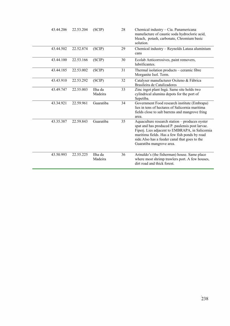
28

43.44.502 29

43.44.206 22.53.204 (SCIP) Chemical industry – Cia. Panamericana manufacture of caustic soda hydrocloric acid, bleach, potash, carbonate, Chromium basic solution.

22.52.874 (SCIP) Chemical industry – Reynolds Latasa aluminium cans

43.44.100 22.53.166 (SCIP) 30 Ecolab Anticorrosives, paint removers, lubrificantes.

43.44.185 22.53.002 (SCIP) 31 Thermal isolation products – ceramic fibre Morganite Isol. Term.

43.43.910 22.53.292 (SCIP) 32 Catalyser manufacturer Oxiteno & Fábrica Brasileira de Catalizadores

43.49.747 22.55.003 Ilha da Madeira

33 Zinc ingot plant Ingá. Same site holds two cylindrical alumina depots for the port of Sepetiba.

43.34.921 22.59.961 Guaratiba 34 Government Food research institute (Embrapa) lies in tens of hectares of Salicornia maritima fields close to salt barrens and mangrove fring area.

43.35.387 22.59.843 Guaratiba 35 Aquaculture research station – produces oyster spat and has produced P. paulensis post larvae. Fiperj. Lies adjacent to EMBRAPA, in Salicornia maritima fields. Has a few fish ponds by road side.Also has a feeder canal that goes to the Guaratiba mangrove area.

43.50.993 22.55.225 Ilha da Madeira

36 Arinaldo’s (the fisherman) house. Same place where most shrimp trawlers port. A few houses, dirt road and thick forest.



238

Appendix 7. Fish species commonly found in Sepetiba Bay (Andreatta, 1997).

Family Species Ariidae Genidens genidens; Bagre marinus; Sciadeichthys luniscutis; Arius spixii Atherinidae Xenomelaniris brasiliensis Belonidae Strongylura timucu; Strongylura marina Bothidae

Trachinotus falcatus; Trachinotus goodei; Trachinotus carolinus; Oligoplites saurus; Oligoplites saliens; Uraspis secunda; Selene setapinnis; Chloroscombrus chrysurus; Caranx crysas; Pseudocaranx dentex; Selene vomer; Selene spixii; Hemicaranx amblyrhynchus

Cynoglossidae Dasyatis guttata; Dasyatis centroura; Gymnura altavela

Ephippididae Diapterus rhombeus; Diapterus richii; Gerres aprion; Gerres lefroyi; Gerres gula; Gerres melanopterus;

Mugilidae Lycodontis ocelatus

Rajidae Psammobatis sp.; Raja castelnaui; Raja agassizi

Soleidae

Syngnathidae

Synodontidae Synodus foctens

Trichimidae

Citharichthys spilopterus; Citharichthys arenaceus; Etropus crossotus; Etropus intermedius; Syacium micrurum; Syacium papillossum

Carangidae

Centropomidae Centropomus parallelus; Centropomus undecimalis Clupeidae Pellona harroweri; Harengula clupeola

Synphurus plagusia; Symphurus tesselatus Dasyatidae Diodontidae Chilomycterus spinosus; Chilomycterus schoepfi Engraulididae Anchoa tricolor; Anchoa januaria; Anchoa spinifera; Anchoa cubana; Anchoviella

lepidentostole; Cetengraulis edentulus; Engraulis anchoita Chaetodipterus faber

Gerreidae

Gobiidae Gobionellus oceanicus; Gobionellus beleosoma; Gobionellus stigmaticus; Microgobius meeki; Awaous tajasica; Bathigobius soporator

Haemulidae Conodon nobilis; Haemulon steidachneri; Pomadasys corvinaeformis Mugil liza; Mugil curema; Mugil sp.

Muraenidae Narcinidae Narcine brasiliensis Pomatomidae Pomatomus saltator

Rhinobatidae Rhinobatos horkeli Sciaenidae Isopisthus parvipinnis; Cynoscion leiarchus; Paralonchurus brasiliensis; Larimus

breviceps; Menticirrhus americanus; Macrodon oncilidon; Pogonias cromis; Stellifer rastrifer; Stellifer brasiliensis; Stellifer stellifer; Ctenosciaena gracilicirrhus; Micropogonias furnieri; Cynoscion striatus; Cynoscion virescens; Umbrina coroides; Cynoscion microlepidotus

Serranidae Diplectrum radiale; Dules auriga; Diplectrum radiale Achirus lineatus; Achirus fasciatus; Trinectes maculatus paulistanus

Squalidae Squalus cubensis Stromateidae Peprilus paru

Syngnathus dunckeri; Syngnathus pelagicus; Syngnathus rousseau; Hippocampus reidi; Oostethus lineatus

Tetraodontidae Sphoeroides testudineus; Sphoeroides spengleri; Sphoeroides nephelus; Sphoeroides adpersus; Lagocephalus laevigatus

Triglidae Prionotus punctatus Trichurus lepturus



239

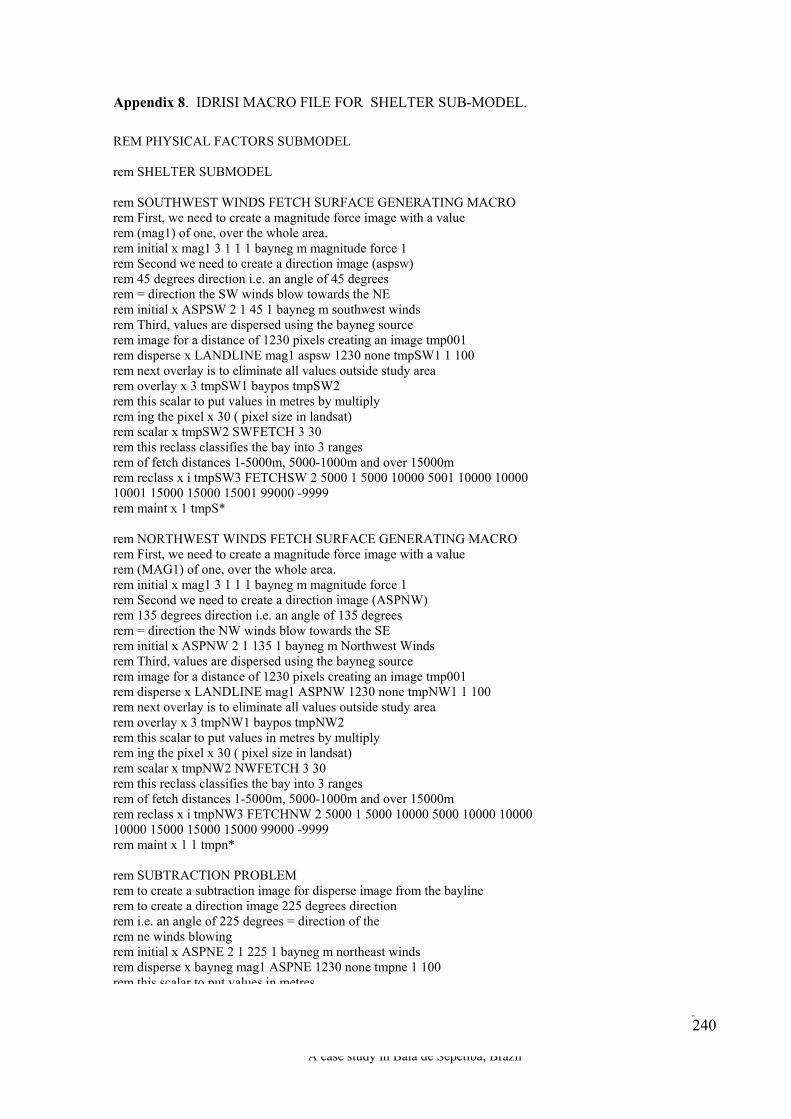
Appendix 8. IDRISI MACRO FILE FOR SHELTER SUB-MODEL.

REM PHYSICAL FACTORS SUBMODEL rem SHELTER SUBMODEL rem SOUTHWEST WINDS FETCH SURFACE GENERATING MACRO rem First, we need to create a magnitude force image with a value rem (mag1) of one, over the whole area. rem initial x mag1 3 1 1 1 bayneg m magnitude force 1 rem Second we need to create a direction image (aspsw) rem 45 degrees direction i.e. an angle of 45 degrees rem = direction the SW winds blow towards the NE rem initial x ASPSW 2 1 45 1 bayneg m southwest winds rem Third, values are dispersed using the bayneg source rem image for a distance of 1230 pixels creating an image tmp001 rem disperse x LANDLINE mag1 aspsw 1230 none tmpSW1 1 100 rem next overlay is to eliminate all values outside study area rem overlay x 3 tmpSW1 baypos tmpSW2 rem this scalar to put values in metres by multiply rem ing the pixel x 30 ( pixel size in landsat) rem scalar x tmpSW2 SWFETCH 3 30 rem this reclass classifies the bay into 3 ranges rem of fetch distances 1-5000m, 5000-1000m and over 15000m rem reclass x i tmpSW3 FETCHSW 2 5000 1 5000 10000 5001 10000 10000 10001 15000 15000 15001 99000 -9999 rem maint x 1 tmpS* rem NORTHWEST WINDS FETCH SURFACE GENERATING MACRO rem First, we need to create a magnitude force image with a value rem (MAG1) of one, over the whole area. rem initial x mag1 3 1 1 1 bayneg m magnitude force 1 rem Second we need to create a direction image (ASPNW) rem 135 degrees direction i.e. an angle of 135 degrees rem = direction the NW winds blow towards the SE rem initial x ASPNW 2 1 135 1 bayneg m Northwest Winds rem Third, values are dispersed using the bayneg source rem image for a distance of 1230 pixels creating an image tmp001 rem disperse x LANDLINE mag1 ASPNW 1230 none tmpNW1 1 100 rem next overlay is to eliminate all values outside study area rem overlay x 3 tmpNW1 baypos tmpNW2 rem this scalar to put values in metres by multiply rem ing the pixel x 30 ( pixel size in landsat) rem scalar x tmpNW2 NWFETCH 3 30 rem this reclass classifies the bay into 3 ranges rem of fetch distances 1-5000m, 5000-1000m and over 15000m rem reclass x i tmpNW3 FETCHNW 2 5000 1 5000 10000 5000 10000 10000 10000 15000 15000 15000 99000 -9999 rem maint x 1 1 tmpn* rem SUBTRACTION PROBLEM rem to create a subtraction image for disperse image from the bayline rem to create a direction image 225 degrees direction rem i.e. an angle of 225 degrees = direction of the rem ne winds blowing rem initial x ASPNE 2 1 225 1 bayneg m northeast winds rem disperse x bayneg mag1 ASPNE 1230 none tmpne 1 100 rem this scalar to put values in metres



240

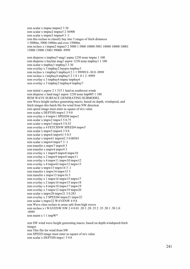
rem scalar x tmpne tmpne2 3 30 rem scalar x tmpne2 tmpne3 2 36900 rem scalar x tmpne3 tmpne4 3 -1 rem this reclass to classify bay into 3 ranges of fetch distances 1-5000m, 5000-1000m and over 15000m rem reclass x i tmpne2 tmpne3 2 5000 1 5000 10000 5001 10000 10000 10001 15000 15000 15001 99000 -9999 rem disperse x tmpbay5 mag1 aspne 1230 none tmpne 1 100 rem disperse x bayline mag1 aspsw 1230 none tmpbay1 1 100 rem scalar x tmpbay1 tmpbay2 3 30 rem overlay x 3 tmpbay2 baypos tmpbay3 rem reclass x i tmpbay3 tmpbay4 2 1 1 99999 0 -30 0 -9999 rem reclass x i tmpbay4 tmpbay5 2 1 0 1 0 1 2 -9999 rem overlay x 3 tmpbay4 tmpne tmpbay6 rem overlay x 3 tmpbay2 tmpbay4 tmpbay7 rem initial x aspsw 2 1 315 1 land m southwest winds rem disperse x land mag1 aspsw 1230 none tmp005 1 100 REM WAVE SURFACE GENERATING SUBMODEL rem Wave height surface generating macro, based on depth, windspeed, and fetch images this batch file for wind from NW direction rem speed image must enter as square of m/s value rem scalar x DEPTHS tmpw1 3 9.8 rem overlay x 4 tmpw1 SPEED4 tmpw2 rem scalar x tmpw2 tmpw3 5 0.75 rem scalar x tmpw3 tmpw4 3 0.53 rem overlay x 4 FETCHNW SPEED4 tmpw5 rem scalar x tmpw5 tmpw6 3 9.8 rem scalar x tmpw6 tmpw61 5 0.5 rem scalar x tmpw61 tmpw62 3 0.00565 rem scalar x tmpw4 tmpw7 3 -1 rem transfor x tmpw7 tmpw8 3 rem transfor x tmpw4 tmpw9 3 rem overlay x 1 tmpw9 tmpw8 tmpw10 rem overlay x 2 tmpw9 tmpw8 tmpw11 rem overlay x 4 tmpw11 tmpw10 tmpw12 rem overlay x 4 tmpw62 tmpw12 tmpw13 rem scalar x tmpw13 tmpw14 3 -1 rem transfor x tmpw14 tmpw15 3 rem transfor x tmpw13 tmpw16 3 rem overlay x 1 tmpw16 tmpw15 tmpw17 rem overlay x 2 tmpw16 tmpw15 tmpw18 rem overlay x 4 tmpw18 tmpw17 tmpw19 rem overlay x 3 tmpw12 tmpw19 tmpw20 rem scalar x tmpw20 tmpw21 3 0.283 rem overlay x 3 SPEED4 tmpw21 tmpw22 rem scalar x tmpw22 WAVENW 4 9.8 rem Wave class reclass to areas safe from high waves rem reclass x i WAVENW NW 2 4 0.01 .20 3 .20 .35 2 .35 .50 1 .50 1.0 -9999 rem maint x 1 1 tmpW* rem SW wind wave height generating macro, based on depth-windspeed-fetch images rem This file for wind from SW rem SPEED image must enter as square of m/s value rem scalar x DEPTHS tmpx1 3 9.8



241

rem overlay x 4 tmpx1 speed3 tmpx2 rem scalar x tmpx2 tmpx3 5 0.75 rem scalar x tmpx3 tmpx4 3 0.53 rem overlay x 4 FETCHSW speed3 tmpx5 rem scalar x tmpx5 tmpx6 3 9.8 rem scalar x tmpx6 tmpx61 5 0.5 rem scalar x tmpx61 tmpx62 3 0.00565 rem scalar x tmpx4 tmpx7 3 -1 rem transfor x tmpx7 tmpx8 3 rem transfor x tmpx4 tmpx9 3 rem overlay x 1 tmpx9 tmpx8 tmpx10 rem overlay x 2 tmpx9 tmpx8 tmpx11 rem overlay x 4 tmpx11 tmpx10 tmpx12 rem overlay x 4 tmpx62 tmpx12 tmpx13 rem Scalar x tmpx13 tmpx14 3 -1 rem transfor x tmpx14 tmpx15 3 rem transfor x tmpx13 tmpx16 3 rem overlay x 1 tmpx16 tmpx15 tmpx17 rem overlay x 2 tmpx16 tmpx15 tmpx18 rem overlay x 4 tmpx18 tmpx17 tmpx19 rem overlay x 3 tmpx12 tmpx19 tmpx20 rem scalar x tmpx20 tmpx21 3 0.283 rem overlay x 3 SPEED3 tmpx21 tmpx22 rem scalar x tmpx22 WAVESW 4 9.8 rem Wave class reclass to areas safe from high waves rem rem reclass WAVESW SW (4) 0.01 .20 (3) .20 .35 (2) .35 .50 (1) .50 1.0 -9999 rem reclass x i WAVESW SW 2 4 0.01 .20 3 .20 .35 2 .35 .50 1 .50 1.0 -9999 rem maint x 1 1 tmpX* REM SUBMODEL PROTECTED FROM WAVES from NW and SW quarters = WAVEOK rem overlay x 8 SW NW WAVEOK rem reclass x i waveok wavedis 2 1 4 6 2 3 4 3 2 3 4 1 2 -9999 rem map and bmp file = wavedis



242

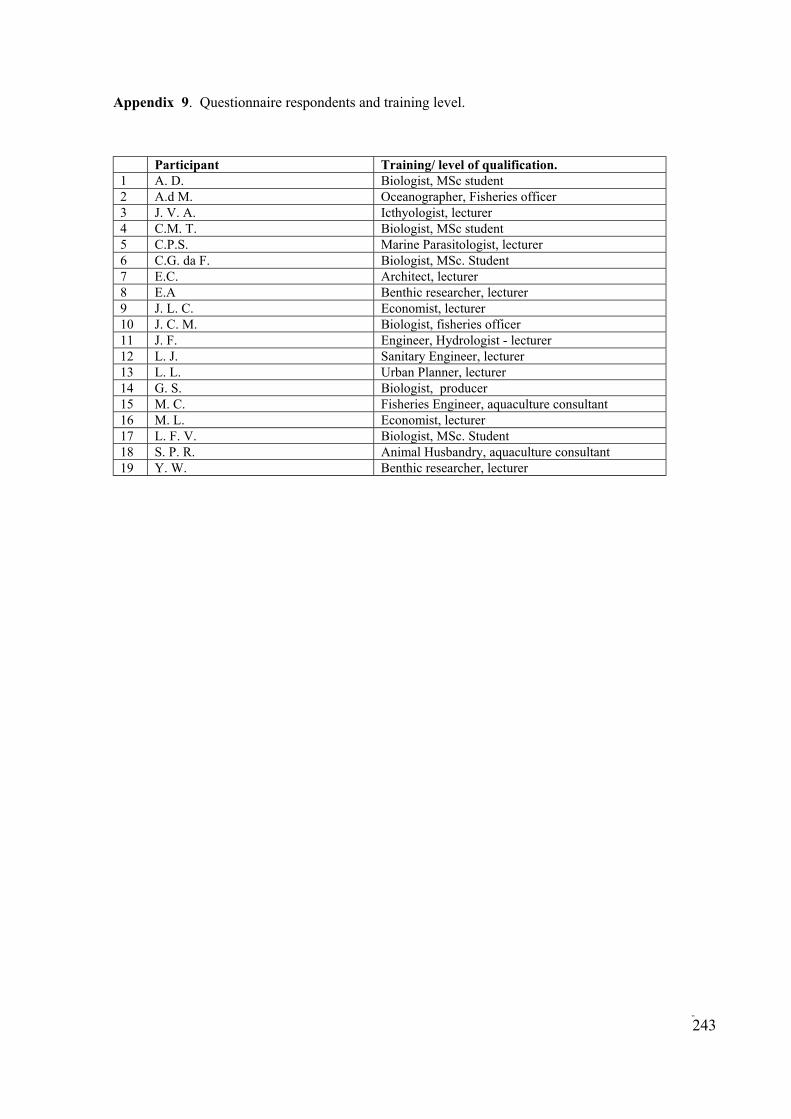
Appendix 9. Questionnaire respondents and training level.

Participant Training/ level of qualification. 1 A. D. Biologist, MSc student 2 A.d M. Oceanographer, Fisheries officer

J. V. A. Icthyologist, lecturer 4 C.M. T. Biologist, MSc student

C.P.S. Marine Parasitologist, lecturer 6 C.G. da F. Biologist, MSc. Student 7 E.C. Architect, lecturer 8 E.A Benthic researcher, lecturer 9 J. L. C. Economist, lecturer 10 J. C. M. Biologist, fisheries officer 11 J. F. Engineer, Hydrologist - lecturer

Sanitary Engineer, lecturer 13 L. L. Urban Planner, lecturer

G. S. Biologist, producer 15 M. C. Fisheries Engineer, aquaculture consultant 16 M. L. Economist, lecturer 17 L. F. V. Biologist, MSc. Student 18 S. P. R. Animal Husbandry, aquaculture consultant 19 Y. W. Benthic researcher, lecturer

3

5

12 L. J.

14



243

Appendix 10. Constrainsts and production factors identified by respondents in questionnaire.

Identified factor Reclassification Hits.

agriculture density Constraint 1 Area available Constraint 1 conflicts, other uses of area Constraint 4 conflicts, traditional fishermen Constraint 1 conservation areas Constraint 1 credit lines Constraint 1 hydrographic basin Constraint 1 Industrial density Constraint 1 Legislation Constraint 4 marine mammal routes Constraint 1 Navigation Constraint 1 Pollution, general Constraint 7 pollution, heavy metals Constraint 3 pollution, industrial Constraint 3 pollution, pesticides Constraint 1 pollution, sewage Constraint 4 sediment quality Constraint 3 Communications Infra 1 Depuration facilities Infra 1 distance, to roads Infra 4

Infra 3 electric power Infra 2 extension/technical support Infra 4 Fishermen organization Infra 1 Infra-structure, general Infra 2 labour availability Infra 3 labour, trained Infra 4

Infra 1 security (theft) Infra 1 seed availability Infra 5 species selection & know-how Infra 4 tradition, fishermen, aquaculture Infra 2 Transportation Infra 1 distance, from land Market 4

Market 7 market, fish consumption Market 1 market, general Market 1 market, Income per capita Market 1 market, product acceptance Market 4 Market, product price Market 2 Population density Market 1

Not applicable 4 macroalgae presence Not applicable 1

2 1 2

Climate Physical 4 coastline contour Physical 1

2 4 3 1

distance, to suppliers

research, insufficient

distance, to consumers

investment costs

Parasites Not applicable Political will power Not applicable Species, competitors Not applicable



244

Predators Physical Production, "natural" capacity Physical Rainfall Physical Relief Physical

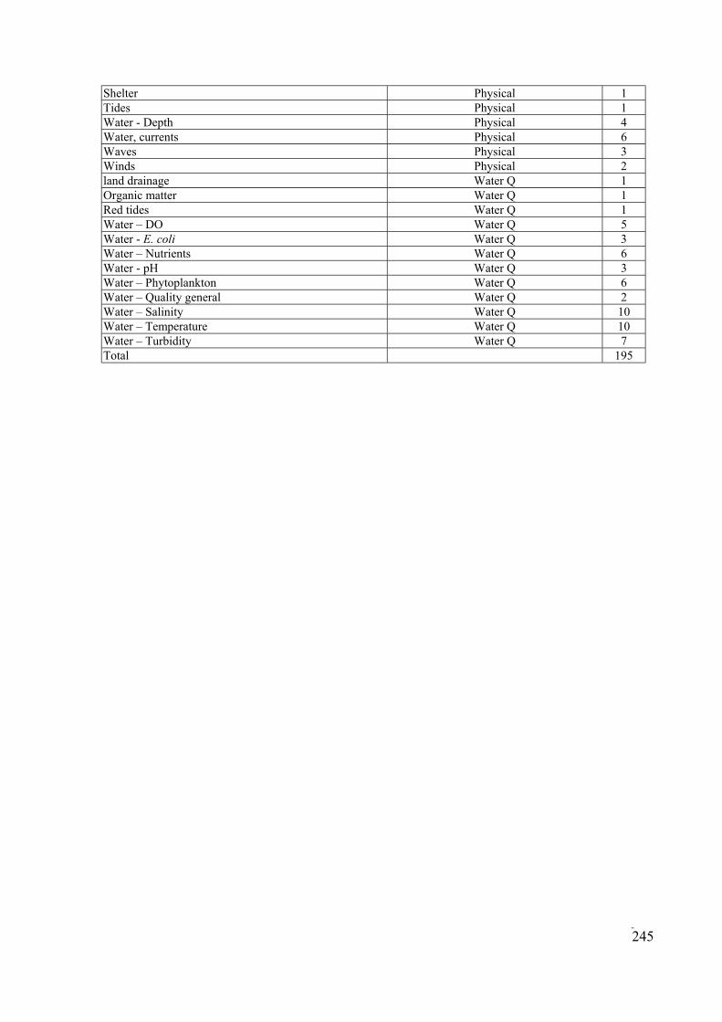
Shelter Physical 1 Tides Physical 1

Physical 4 6 3

Winds Physical 2 1 1 1 5 3 6

Water - pH Water Q 3 Water – Phytoplankton Water Q

Water Q 2 Water – Salinity Water Q 10 Water – Temperature Water Q 10 Water – Turbidity Water Q 7 Total 195

Water - Depth Water, currents Physical Waves Physical

land drainage Water Q Organic matter Water Q Red tides Water Q Water – DO Water Q Water - E. coli Water Q Water – Nutrients Water Q

6 Water – Quality general



245

gis - brazil_ thesis

Documents