Giordano Mion Spatial externalities and empirical analysis: the case of Italy Article (Accepted version) (Refereed)

Original citation: Mion, Giordano (2004) Spatial externalities and empirical analysis: the case of Italy. Journal of urban economics, 56 (1). pp. 97-118. ISSN 0094-1190 DOI: 10.1016/j.jue.2004.03.004 © 2004 Elsevier This version available at: http://eprints.lse.ac.uk/42663/ Available in LSE Research Online: May 2012 LSE has developed LSE Research Online so that users may access research output of the School. Copyright © and Moral Rights for the papers on this site are retained by the individual authors and/or other copyright owners. Users may download and/or print one copy of any article(s) in LSE Research Online to facilitate their private study or for non-commercial research. You may not engage in further distribution of the material or use it for any profit-making activities or any commercial gain. You may freely distribute the URL (http://eprints.lse.ac.uk) of the LSE Research Online website. This document is the author’s final manuscript accepted version of the journal article, incorporating any revisions agreed during the peer review process. Some differences between this version and the published version may remain. You are advised to consult the publisher’s version if you wish to cite from it.

Spatial Externalities and Empirical Analysis: The Case of Italy∗

Giordano Mion†

January 2004

Abstract

This paper aims at assessing the role of market linkages in shaping the spatial distribution of

earnings. Using a space-time panel data on Italian provinces, I structurally estimate a NEG model in

order to both test the coherence of theory with data, as well as to give a measure of the extent of spatial

externalities. Particular attention has been paid to those endogeneity issues that arise when dealing

with both structural models and spatial data. Results suggest that final demand linkages influence the

location of economic activities and that their spread over space is, contrary to previous findings, not

negligible.

Keywords: Economic Geography, Spatial Externalities, Market Potential.

JEL Codes: F12, R12, R32.

∗I thank Salvador Barrios, Luisito Bertinelli, Miren Lafourcade, Andrea Lamorgese, Thierry Magnac, Thierry Mayer,Dominique Peeters, Susana Peralta, Antonio Teixeira, Jaçques Thisse and LASERE seminar participants at CORE forhelpful comments and suggestions. I am also grateful to Claire Dujardin, Ornella Montalbano, and Renato Santelia forproviding me with local data on distances and economic indicators.

†Giordano Mion: CORE (Université Catholique de Louvain-la-Neuve, Belgium), and Dipartimento di Scienze Economiche(University of Bari, Italy). Address: CORE-UCL, Voie du Roman Pays 34, 1348 LLN, Belgium. Email: mion@core.ucl.ac.be.

1

1 Introduction

Economic activities are certainly not equally distributed across space. However, despite some interesting

early contributions made by Hirschman, Perroux or Myrdal, this issue remained largely unaddressed by

mainstream economic theory for a long while. As argued by Krugman [26], this is probably because

economists lacked a model embracing both increasing returns and imperfect competition in a general

equilibrium framework.

The relatively recent new economic geography literature (NEG) has finally provided a collection of

general equilibrium models explicitly dealing with space, and able to account for many salient features of

the economic landscape.1 As Krugman [26] pointed out, there is a strong connection between the NEG

and some older fields in economics. To a large extent, what has been done is in fact rediscovering concepts

and ideas that did not receive much attention by mainstream economic theory because of their lack of

a rigorous formal counterpart. Within this group of overlooked contributions, and of particular interest

for this paper, is the literature on market potential starting with Harris [19]. This strand of literature

argues that a location’s attractiveness for firms depends on its access to markets. The quality of this

access is often measured by an index of market potential, which is a weighted sum of the purchasing power

of all other locations, with weights inversely related to distance. Although this approach has proved to

be empirically quite powerful, it totally lacked any microeconomic foundation. At that time, there were

in fact no rigorous explanations of why a correlation between market access and firms’ location should

exists. However, Fujita, Krugman and Venables [15] show that market potential functions can be obtained

from spatial general-equilibrium models, thus providing the theoretical background for the use of such an

approach.

The main objective of this paper is thus to estimate a market potential function, derived from a NEG

model, using data for Italian provinces. The particular framework used is a multi-location extension of

Helpman [22] two-location model, originally introduced and estimated by Hanson [17] for the US counties,

in order to:

1. Obtain estimates of structural parameters to infer the consistency of Helpman’s model with reality.

2. Evaluate the theory-based market potential function in the light of the empirical literature on market

potential, in order to investigate the specific contribution of the model in understanding firms’

location.

3. Give an idea of the extent of spatial externalities by measuring how far in space a shock in one

location affect the others.

I depart from the the existing literature, and in particular from Hanson [17], in several ways. First,

a rigorous estimation technique, derived from Spatial Econometrics and Dynamic Panel Data, have been

implemented in order to tackle some unaddressed endogeneity issues that naturally arise when dealing with

1See Fujita and Thisse [14], Ottaviano and Puga [28], and Fujita, Krugman and Venables [15] for a review of the literature.

2

structural spatial models. Second, I introduce a new measure of equilibrium local wages that is needed in

order to account for those structural differences, like labor mobility, that make international comparisons

of agglomeration forces problematic. Finally, I make use of several distance decay functions in order to

investigate the sensitivity of my results to the particular assumption made about transportation technology.

Interestingly, in my preferred specification, the results indicate that the spatial scope of agglomeration

externalities is larger than what emerges from former studies.

This paper contributes to the growing empirical literature on the location of economic activities. There

are, however, different approaches in this research field, each relying on a different agglomeration mech-

anism.2 Agents may in fact be drawn to regions with pleasant weather or other exogenous amenities.3

However, both human capital accumulation stories4 and localized spillovers, like Marshall or Jacobs ex-

ternalities, may also contribute to geographic concentration.5 By contrast, here I stress increasing returns

and market interactions, as opposed to factor endowments (exogenous amenities) and technological exter-

nalities (human capital and technological spillovers), taking the NEG framework as the theoretical basis

for my investigations. Other examples of this market-linkages approach can be found in Combes and

Lafourcade [8], Head and Mayer [21], and Teixeira [37].

The rest of the paper is organized as follows. In Section 2 I give some insight on the mechanics of

Helpman [22] model, and I present the structural equation that I will estimate. Section 3 deals with data

issues, while in Section 4 I discuss econometric concerns. Detailed estimation results are presented in

Section 5. Finally, in Section 6 I draw some conclusions and suggest directions for further research.

2 NEG and Market Potential

The NEG literature offers the possibility to treat agglomeration in a flexible and rigorous way by means

of increasing returns (IRS), imperfect competition, and product differentiation. In this Section, I am

particularly concerned with Helpman’s [22] model, which will be the theoretical ground on which I will

construct the econometric analysis.6

Helpman’s [22] model is actually a two-good, two-factor, two-region model that closely resembles the

well-known core-periphery model by Krugman [25]. In both cases, there is an IRS manufacturing sector,

producing a differentiated product under monopolistic competition, where the only input is an inter-

regionally mobile workforce. Workers/consumers migrate from one region to another according to differ-

ences in real wages, while firms look for high profitable locations. However, while in Krugman [25] the

other good is homogenous, freely tradable and produced under constant returns to scale (CRS) by a sector

specific immobile labor force (farmers), in Helpman [22] it is instead a non tradable good (like housing

services) that is produced with an exogenously distributed sector specific capital under CRS. As for the

2See Hanson [18] for a survey of the empirical literature on agglomeration economies.3 See for example Rosen [33], and Roback [32].4 See Lucas [27], and Black and Henderson [6].5As for the impact of localized externalities on productivity and growth see Henderson, Kuncoro, and Turner [24], and

Ciccone and Hall [7].6 For a detailed exposition of the model, see Helpman [22] and Hanson [17].

3

distribution of capital ownership, in Helpman [22] this is supposed to be public, i.e. each individual mobile

worker/consumer owns an equal share of the total capital/housing stock H. Equilibrium real wages are

equalized across regions unless some areas become empty. Contrary to Krugman [25], this is, however, a

very unlikely outcome because it implies that in abandoned regions the price of housing is zero. Therefore,

locations where manufacturing activities agglomerate are characterized by high housing prices, and this

act as a dispersion force against the tendency for firms to concentrate close to big markets (the so-called

market access effect).

Depending on the level of transportation costs (f), elasticity of substitution among varieties (σ) and

the share of traded goods in consumers’ expenditure (µ), manufacturing activities will be dispersed or

agglomerated. In the second case firms will be disproportionately distributed with respect to a region size.

In particular, indicating with (Hi) the stock of housing of region i, those locations with an above (below)

average endowment will have a more (less) than proportional share of manufacturing in equilibrium. Both

a higher share of tradable goods (µ) or a lower elasticity (σ) induce more agglomeration. In the case

of µ, this is due to the fact that concentration of firms and consumers in the same place allow to avoid

transportation costs thus increasing real consumption. The greater is the share of these goods in the

consumption of migrating workers, the stronger is this centripetal force. The role of σ is instead to

counterbalance the usual centrifugal force that works against concentration: price competition. A lower

elasticity of substitution σ makes in fact varieties more differentiated, relaxing local competition among

sellers.

There are basically two reason for which I prefer to use Helpman instead of Krugman model for my

empirical investigation of Italian provinces. First of all, Helpman’s model seems to be more suitable to

describe the kind of forces at work at low-level spatial scale, where congestion costs and the price of land

are key localization factors for both firms and consumers. In particular, the fact that in Krugman [25]

equilibrium nominal wages are lower in regions where agglomeration takes place is particularly disturbing.

Moreover, from an empirical point of view, Helpman [22] is also preferable because of the less extreme nature

of its equilibria. Although the production of manufactured tradables is certainly highly agglomerated in

space, the full concentration in very few places, that is quite a standard outcome in Krugman [25], is far

too extreme.

In order to give a useful interpretation of the kind of investigations I want to deal with, as well as to

link them to previous studies, one has to come back to Harris’s [19] market-potential concept. Actually,

Harris’s [19] market-potential relates the potential demand for goods and services produced in a location

i = 1, 2, ..,Φ to that location’s proximity to consumer’s markets, or:

MPi =ΦXk=1

Ykg(dik) (1)

where MPi is the market potential of location i, Yk is an index of purchasing capacity of location k

(usually income), dikis the distance between two generic locations i and k and g() is a decreasing function.

The higher is the market potential index of a location, the higher is its attraction power on production

activities.

4

In Helpman’s model, a good measure of the attractiveness of location i is given by the equilibrium

nominal wages wi. Although firms makes no profits in equilibrium (no matter where they are located),

the wage they can afford expresses their capacity to create value once located in a particular region. In

fact, if centripetal forces take over, those locations that attract more firms and consumers will also have

higher equilibrium nominal wages, thus leading to a positive correlation between agents’ concentration and

wi. Following Hanson [17], one can combine some equilibrium equations and apply logarithms to simplify

things in order to get the following expression for ln(wi):

ln(wi) = κ3 + σ−1 ln

"ΦXk=1

Y1−σ(1−µ)

µ

k H(1−µ)(σ−1)

µ

k w(σ−1)µ

k f (di,k)(σ−1)

#(2)

where κ3 is a function of behavioral parameters (µ, σ), and f() is, for the moment, a generic decreasing

function of distance that I will parametrize explicitly afterwards.

Equation (2) really looks like a market-potential function. It tells us that as long as agglomeration

forces are active (σ(1− µ) < 1), the nominal wage in location i (and thus local firms’ profitability) is an

increasing function of the weighted purchasing power coming from surrounding locations (Yk), with weights

inversely related to distances dik trough the transport technology function f(.) (this is the market access

component). Crucially, (2) tells us more than the simple market potential equation (1). The distribution

of economic activities should in fact depend upon prices, because an increase in other locations’ housing

stock (Hk) or wages(wk), causes wi to increase in the long-run in order to compensate workers for lower

housing prices and higher earnings they can enjoy elsewhere. Although quite powerful from an empirical

point of view, relations like (1) were not obtained from a theoretical model and, compared to (2), did not

control for wages and prices of others locations.

3 From Theory to Econometrics: Data Issues

One of the most common problems in using micro-founded economic models for empirical purposes is

the choice of good proxies. Estimation requires actual data, and in some circumstances the choice of the

statistic that is best suited to approximate a theoretical variable becomes a difficult task. As for the case

of equation (2), the variables H, Y , and d do not raise particular interpretation problems. H is meant

to represent those goods and factors that are immobile for consumption or production. Expenditure on

housing services actually constitutes a large part of these costs. A good proxy is thus given by the total

size of houses available (for both for family and commercial use) in a region measured in square meters.

The variable Y should instead represent the demand for goods, and a reasonable solution is to take total

household disposable income as a measure of province’s purchasing power. Finally, d is the distance

between two generic locations. The unavailability of more sophisticated measures of distance has led us to

use a physical metric. In particular I adopt the crow flight distance between the centers of each province

(as obtain by polygonal approximation) using GIS software.

However, when one thinks about w some complication arise. One natural solution, followed by Hanson

5

[17], is to consider it as just labor income, thus using county statistics on average earnings of wage and

salary workers. Although this solution may be to some extent acceptable for the US, it seems difficult to

argue the same for Europe and in particular for Italy. First, it is a wide spread opinion that in Europe

conditions of local supply and demand play little role in the determination of wages7, thus making them

unsuited to express re-location incentives. In some countries, and this is the case for Italy, wages are in

fact set at the national level for many production sectors. Second, the relatively scarce mobility of people

prevents the price system to clear labor markets excess-supply.8 Agglomeration externalities are thus likely

to magnify regional imbalances in both income and unemployment rates rather than shifting massively

production activities.

In line with these considerations, US economic activities are more spatially concentrated than in Eu-

rope. The 27 EU regions with highest manufacturing employment density account for nearly one half of

manufacturing employment in the Union and for 17% of the Union’s total surface and 45% of its pop-

ulation. The 14 US States with highest manufacturing employment density also account for nearly one

half of the countries manufacturing employment, but with much smaller shares of its total surface (13%)

and population (21%). By contrast, in Europe agglomeration is more a matter of income disparities and

unemployment. 25% of EU citizens live in so-called Objective 1 regions. These are regions whose Gross

Domestic Product per capita is below 75% of the Unions average. By contrast only two US states (Missis-

sippi and West Virginia) have a Gross State Product per capita below 75% of the country’s average, and

together they account for less than 2% of the US population. Moreover, regional employment imbalances

are a special feature of European economic space. The case of Italy is best known, with Campania having

a 1996 unemployment rate 4.4 times as high as Valle d’Aosta. However, as shown by Overman and Puga

[30], large regional differences exist in all European countries.

These considerations suggest the existence of similar forces shaping the distribution of economic activ-

ities in an asymmetric way. The point is that the structural differences between US and EU cause these

forces to have a more visible impact on different economic indicators. At this stage, it is probably better

to come back to Helpman [22] to look for some guiding insights. In that framework, w is the zero-profit

earnings of the only production factor for tradables (labor), and it turns out to be a measure of the at-

tractiveness of a location for firms. As long as mobility is limited, the transfer of firms in some locations

would produce unemployment in the abandoned ones while pushing the factor market to full employment

in the former. However, the fact that basic wages are more or less fixed does not prevent firms to give

workers, if they have the means, other form of remunerations in order to attract them. Therefore, one can

think to use total labor expenditure per employee as a measure of the shadow wage. However, labor is not

the only production factor in real world. In Helpman [22] it stands for the aggregate of mobile factors,

as opposed to the immobile ones (H), and so mobile capital remunerations should also be included in the

construction of a good proxy. Furthermore, profits need also to be accounted for as they are, in principle,

precisely those indicators leading firms to relocate. In this light, it thus seems problematic to associate w

7 See Bentolila and Dolado [4], and Bentolila and Jimeno [5] for an empirical assessment.8Eichengreen [11] estimates that the elasticity of interregional migration with respect to the ratio of local wages to the

national average is 25 times higher in the US than in Britain. The difference with respect to Italy is even larger.

6

to wages only, and this criticism apply to the US case too.

The solution I will adopt tries to address these issues. First, in order to be consistent with Helpman’s

model, remuneration of immobile capital should not enter in the computation of w. The reason is that

w should measure the incentive for mobile factors (labor in Helpman [22]) to move towards agglomerated

areas. Expenditure in housing services actually represent a large part of those remuneration. Therefore,

using statistics on rented house numbers and prices from the Italian National Institute of Statistics (IS-

TAT), I have constructed a measure of housing spending per province and, after subtracting it from GDP,

I have divided by active population (to control for different unemployment rates) to get my w.9 The

variable obtained is meant to capture the average remuneration of all mobile factors, as well as profits,

and it is only indirectly related to local wages. In Section 5, I will provide further (empirical) evidence to

justify my measure of w for the Italian economy.

Table 1 contains summary statistics on w, H, and Y , as well as on provinces’ surface and their popu-

lation. All nominal variables are in 1996 prices and the unit is one million liras. Total housing area H is

measured in square meters, while population is in thousands of people and provinces area is expressed in

square kilometers. Data are time-averaged and refer to the interval 1991-1998. Statistics on rented-house

numbers and prices come from ISTAT. Data on GDP, population, employees, housing stock, and house-

holds’ disposable income come from SINIT database (Sistema Informativo per gli Investimenti Territoriali).

The latter data-set has been collected from the “Dipartimento Politiche di Sviluppo e Coesione - Ministero

dell’Economia e Finanze”. Finally, distances have been obtained with GIS software and are expressed in

kilometers.

4 Econometric Specification

4.1 Main Concerns

As mentioned in the Introduction, the main goal of this paper is to estimated a structural model and in

particular equation (2). However, the data-set I have is a panel covering two dimensions: space and time.

Therefore, the actual formulation I use is:

ln(wi,t) = κ3 + σ−1 ln

"ΦXk=1

Y1−σ(1−µ)

µ

k,t H(1−µ)(σ−1)

µ

k,t w(σ−1)µ

k,t f (di,k)(σ−1)

#+ εi,t (3)

where indexes i and t corresponds, respectively, to space and time, while εi,t is a random term that, for

the moment, is just assumed to be serially uncorrelated in the time dimension, that is Cov(εi,t, εi,s) =

0, ∀ t 6= s. Later on, I will explicitly test this assumption.

The first choice to make is the geographical reference unit. On one hand, this should not be too

large in order to account for the nature of externalities that the model wants to capture. Helpman [22]

9Actually, I subtract people looking for their first job from active population before computing w. The number of thoselooking for their first occupation is in fact closely related to factors (like social habitudes), that are both external to themodel and vary a lot across Italy, thus introducing a potential source of bias.

7

is in fact best suited to describe agglomeration forces at low/medium scale spatial level. The tension

between easy access to cheap commodities and high costs of non-tradable services like housing is certainly

a good metaphor for metropolitan areas, but the more one departs from this example the more other forces

are likely to be at work. On the other hand, a too high geographical detail could also misrepresent the

tensions at work, as well as to requiring an intractable amount of information. To give an example, if one

decides to work on the approximately 8, 100 Italian municipalities, he will need a matrix of distances with

8, 100 ∗ (8, 100 + 1)/2 = 32, 809, 050 free elements to evaluate. My choice is thus a compromise betweenthese two different needs, and consists in taking the 103 Italian provinces as reference units.

Turning to specification issues, I should argue why I choose (2) in order to get the estimates of structural

parameters. In principle, this objective would be better achieved using simultaneous equations techniques

directly on Helpman [22] equilibrium equations. However, apart from implementation difficulties, it is

the unavailability of reliable statistics for manufacturing goods at any interesting geographical level that

makes this solution unapplicable. Data on prices can in fact be found at the regional level for Italy. This is

probably too much an aggregate unit for my purposes because of the lower inter-regional labor mobility, as

well as the limited number of cross-section observations (just 20). Equation (2) is instead a reduced-form,

in an algebraic sense, of the model that does not contain these two variables, and for which it is thus

possible to find adequate local data.

Another important aspect concerns missing variables like local amenities (nice weather, ports, road

hubs, etc.) and localized externalities (especially human capital ones), that possibly influence the distri-

bution of earnings, but are not included in the analysis. As long as these variables are correlated with

regressors, and they are indeed likely to be, standard econometric techniques would fail. Anyway, when

one thinks about both amenities and externalities it is clear that, if these factors change over time, their

variation is very slow. The quality of the work force, as well as the presence of infrastructure and the

network of knowledge exchange is thus reasonably constant (for a given location) in a short interval of

time. I can thus try to overcome this problem with an appropriate choice of the estimation interval, (that

should not be too long) in order to treat them as correlated fixed effects µi. The random term would thus

become εi,t = µi + ui,t and, applying a time-difference on (3), the term 4εi,t = εi,t − εi,t−1 would then

simplify to the time-varying component difference only: 4ui,t = ui,t − ui,t−1.10

To actually implement estimations, one needs to define define distance weights f (di,k) in equation (3).

These weights should measure the degree of economic interaction among locations. Actually, Hanson [17]

uses the exponential form f (di,k) = exp−τdik , where τ ∈ [0,∞) is an (inverse) measure of transportationcosts to be estimated, and di,k is distance between i and k. However, such a specification gives rise to some

odd results. For example, according to Hanson’s [17] estimates, travelling two km appears to multiply the

price of a good by 50. This quite unrealistic result comes from the fact that an inverse exponential goes

to zero very fast (faster than any polynomial function). Therefore, as a robustness check, I will try an

alternative specification that is more rooted in trade theory analysis: the power function f (di,k) = θ dψi,k.

10 It is worth noting that localized externalities need a model where production is disaggregated by sector in order to becaptured. In fact, Marshall and Jacobs’s externalities are usually measure by indexes of (respectively) industrial specializationand diversification. Therefore, it seems problematic to include them in my aggregate model.

8

Helpman [22] is essentially a trade model, so that a good proxy for economic interaction is given by trade

flows. In this respect, the power function has been extensively used in both gravity equation and home

bias literature11 . Comparing results obtained with these two measures, and in particular the associated

goodness of fit, will help us to shed some light on the spatial scope of agglomeration externalities.12 As a

further check on the pervasiveness of final-demand linkages, I will also perform some unstructured linear

estimations using many distance-band matrices in the same spirit as Rosenthal and Strange [35] and

Henderson [23].

A final issue is related to endogeneity. First, the presence on the right hand side of a weighted sum

over space of the same variable appearing as independent (wi,t), is a source of bias. According to spatial

econometrics, this sum can be seen as a spatially-lagged endogenous variable and it is well known that,

in this case, the least squares method does not work regardless of error properties13. Furthermore, in

my structural model, wi,t is determined simultaneously with income Yi,t. The circularity between factor

earnings and income is certainly not debatable in economic theory, and in my framework implies that

the explanatory variable Yi,t is correlated with disturbances ui,t. Finally, even if the amount of fixed

factors Hi,t is supposed to be exogenous in Helpman model, it is not difficult to imagine that, for example,

pressures on the housing market do not simply lead to price movements, but also encourage construction

of new buildings.

The solution proposed by Hanson [17] to account for endogeneity is to use aggregated spatial variables

as regressors on the right hand side of equation (3), and then apply non-linear least squares (NLLS).

Following his reasoning, ui,t should in fact reflect temporary shocks that influence local business cycles.

The finer the geographical unit I use for locations, the smaller is the impact of such shocks on geographically

aggregated variables. Furthermore, if these shocks are really local, their spread to other regions should be

negligible. Now, if this is true, then there should not be any significant correlation between the shock ui,t

of a small county i and (for example) the state-level values of w, Y , and H. Actually, Hanson [17] uses

data on w for the 3075 US counties as dependent variables and, for each county i, he uses data on w, Y , H

and distances at the state level as independent variables on the right hand side of (3). Formally speaking,

the two indexes i and k do not correspond anymore to the same location set, with index i = 1, 2...,Φ

corresponding to US counties, and k = 1, 2, ...,Φ∗ corresponding to US states.14

A few considerations are in order. Hanson’s idea sounds like instrumentation. He actually employs

state level values on the right-hand side precisely because he needs something that is uncorrelated with

the disturbances, but still linked with the (real) explanatory variables at county level. Indeed, these are

the features of good instrumental variables. Therefore, as an alternative estimation methodology, one can

11See Disdiez and Head [10].12 In order to make spatial econometrics techniques directly applicable I will estimate θ, while using for ψ values coming

from the literature. The distance weight f¡di,k

¢in (3) is raised to the power σ − 1, and so I am actually interested in

ψ (σ − 1). Following Disdiez and Head [10], a reasonable estimate for ψ (σ − 1) is −1, so that the distance decay I will useis: f

¡di,k

¢σ−1= θd−1i,k . Furthermore, as standard in spatial econometrics, I will give a zero weight to observations referring

to the same location, i.e. f (di,i)σ−1 = 0.

13 See Anselin [1].14 In equation (3) for instance he has, for a given year t, a sum of Φ∗ = 49 terms (the number of US continental states plus

the district of Columbia) on the right hand side, for each of the Φ = 3075 equations to fit.

9

think of keeping county level variables on the right hand side, and use geographically aggregated data

directly as instruments for the estimation. Clearly, as long as Hanson’s strategy works, the other should

work as well. Furthermore, a non-linear instrumental variable approach (NLIV) would be conceptually

preferable because it allows to maintain a homogeneous space unit on both sides of (3). In the spatial

econometrics literature, it is in fact well known that the level of aggregation matters a lot.15 However,

there is another aspect in favor of instrumental variables: efficiency. By aggregating explanatory variables,

Hanson loses a lot of information, ending with a sum of just 49 terms instead of 3075. By contrast, all the

information contained in county data would be preserved with instrumental variables as one can keep a

fine geographical level also on the right-hand side. I will pay further attention to these two consideration

in the Section devoted to estimation.

There is, anyway, something unclear in the crucial identifying assumption on which the two above

described procedures rely. Technically speaking, they amount to assume that time-varying residuals ui,t

are uncorrelated among themselves as well as with spatially aggregate values of w, Y , and H. The first

assumption is quite clear, and can be tested using spatial econometrics tools like the Moran correlation

test16 . The second is, by contrast, quite obscure and needs to be better clarified. For the shock of

county i to be uncorrelated with the state-level values of w (which are nothing else that averages of the

corresponding Φ county values wi), one needs Cov(ui,t, wk,t) = 0 ∀ i 6= k. In other words, the local shock

does not spread over other locations, resulting in a negligible degree of “spatial interaction”. The fact that

error terms are not spatially correlated limits the degree of spatial interaction in the sense that uk,t has,

for example, no impact on wi,t through ui,t because the latter is uncorrelated with uk,t. However, uk,t does

have an impact on wi,t through wk,t because the latter figures as an explanatory variable in (3), and wk,t

is itself a function of uk,t. Therefore, as long as estimates obtained with NLLS or NLIV are significant,

the correlation between uk,t and wi,t through wk,t could not be negligible and aggregate variables cannot

be used as instruments. Put differently, as long as the theoretical model has something interesting to say

about local factor earnings, consumers’ expenditure, and non-tradable goods, then the aggregation trick

does not work.

In the next Subsection I introduce an alternative estimation strategy, that can potentially be used for

many spatial structural models applications, in order to properly address endogeneity.

4.2 Escaping the Endogeneity Trap

A possible way-out from this endogeneity trap that, at the same time, would allow us to preserve the

same space dimension for all variables, could be to better exploit the information coming from the time

dimension, using dynamic panel data à la Arellano and Bond [3]. This basically consists of estimating the

model in first differences (in order to get rid of fixed effects), while using past levels of endogenous variables

15 In order to explore the extent of this possible inhomogeneous data bias, I will perform a comparative estimation usingthe two techniques: a non-linear least squares Hanson type, and a non-linear instrumental variables one.16 See Anselin [1], and Anselin and Kelejian [2].

10

(starting from t− 2) as instruments. However, for this procedure to work correctly, time-dynamics shouldalso be accounted for.

NEG models are designed mainly to reply to theoretical rather than empirical purposes. Compared to

applied macro-economic models, they are in fact represented by systems of equilibrium equations in which

almost all variables are endogenous, making the identification task problematic to solve for a given time

t (i.e. using only the cross-section dimension). This is precisely the reason for which a panel approach

is preferable. Now, since endogeneity comes from the simultaneous nature of these models linking, in

equilibrium, the Φ economies, one can think of using the weak-exogeneity assumption and applying the

appropriate GMM estimator directly to (3). However, such an approach rests on the hypothesis that the

simultaneity problem is fully contemporaneous, ruling out any dynamic behavior.17 In the real world, it is

unlikely that data do not exhibit a time dynamics so that the impact of a shock ui,t is entirely exhausted at

t without spreading over time. For example, frictions in the factors market, like the presence of unobserved

sunk costs for migration or unions’ power, would cause variables to adjust in a sluggish way toward their

equilibrium level, thus justifying the time persistency of a shock. This is why I prefer to resort to dynamic

panel data techniques à la Arellano and Bond [3].

In particular, in order to account for the time dynamics, a time-lagged value of ln(wi,t), as well as a

complete set of time dummies, will be added to regressors in the estimation of (3). As long as tests on

residuals will not detect a significant time correlation, one can be confident that this solution successfully

controls for the time dynamics.18 Then, following Arellano and Bond’s [3] idea, I can apply a first difference

and use past levels of endogenous variables, starting from t−2, as instruments for the estimation. Although,contrary to the usual panel framework, observations are not independent in the cross-section dimension

(and this is a peculiarity of spatial data), convergence is achieved, as showed by Anselin and Kelejian [2],

as Φ goes to infinity if error terms are spatially uncorrelated.

Formally speaking, the set of identifying restrictions on which my procedure relies is:

1. Cov(ui,t, uk,t) = 0∀ i 6= k

2. Cov(ui,t, ui,s) = 0∀ t 6= s

3. E[ui,t|xi,s] = 0∀ t > s

where i, k = 1, 2...,Φ and s, t = 1, 2..., T . The first set of restrictions requires absence of spatial correlation,

and can be investigated by means of a Moran test. The second calls for absence of residual time-dynamics.

The Arellano and Bond [3] GMM estimator is in fact incompatible with disturbances having an AR

17Unreported GMM estimations (based on the weak-exogeneity assumption) on a linearized version of equation (3), supportthe introduction in the model of some dynamic component. In particular, the Sargan test on over-identifying restrictionrejects the validity of instruments and, crucially, the tests on residuals detect a significant time correlation thus suggestingthe presence of a misspecified time-dynamics.18A slightly more general formulation would consist in using an error autoregressive process: ui,t = δui,t−1 + vi,t. I

choose the other one mainly for computational reasons. They both amount to put some time-dynamics in the data, withthe difference being that the in the second the lags of the original regressors should also be introduced in the estimationwith their own (restricted) parameters. These restrictions require the implementation of a non-linear recursive procedure.Furthermore, specification tests did not detect any unaccounted source of endogeneity, suggesting that my choice is a goodcompromise between computational issues and the need to control for time-dynamics.

11

structure: the dynamics need to be captured into the model, as I am trying to do by adding a time-lagged

value of ln(wi,t), as well as a complete set of time dummies, to (3). Tests on the residuals’ time correlation

will then allow investigation of the validity of such an assumption. Finally, the third type of condition

expresses weak exogeneity and, together with the others, makes past values of endogenous variables good

instruments. It is important to stress that, contrary to Hanson’s procedure, the validity of instruments

can be directly assessed here by means of a Sargan test on over-identifying restrictions. Furthermore, my

strategy allows us to keep the same geographical dimension for dependent, explanatory, and instrumental

variables, thus avoiding a possible inhomogeneous data bias.

However, non-linearity of equation (3) is a computational challenge. It certainly complicates the im-

plementation of simple panel techniques but, more importantly, could cause estimations to be extremely

unstable. As known in applied econometrics, the combination of non-linearity, endogeneity, and instru-

mentation is a dangerous mix that causes criterion functions to have many local minima. The solution I

adopt is then to estimate a linearized version of equation (3). This approach is not new for NEG applied

models, and has been pioneered by Combes and Lafourcade [8] with promising results. In an unpublished

Appendix, available from the author upon request, I formally derive the following linear counterpart of (3)

which is given by:

ln(wi,t) = a+ΦXk=1

[(B1Yk,t +B2Hk,t +B3wk,t) d−1i,k )] + εi,t (4)

where B1 = θ 1−σ(1−µ)σµ , B2 = θ (1−µ)(σ−1)σµ , B3 = θσ−1σµ , and for example Yk,t = ln(Yk,t)Yk,tPΦk=1 Yk,t

.

Equation (4) is now linear in the 3 parameters (B1, B2, B3) and, after adding time dummies and a

time-lag of ln(wi,t) to control for time-dynamics, one gets the final regression equation:

ln(wt) = i dumt + ln(wt−1)A+WYtB1 +WHtB2 +WwtB3 + εt (5)

where bold variables are column vectors containing observations for the Φ locations at time t,W is a ΦxΦ

spatial weighting matrix with generic elementWi,k = d−1i,k , i is a vector of ones, and dumt is a time-dummy.

Equation (5) will be the one I will use for my dynamic panel investigations. With estimates of B1, B2,

and B3 in my hands, I can then trace back the implied values of µ, σ, and θ and, using the Delta method,

make inferences on the latter.

To account for possible structural differences between continental Italy and the two islands of Sicily and

Sardinia, I compute estimates using continental provinces only. Further details about spatial aggregation

and instruments are given in the Appendix.

12

5 Estimations

5.1 Regressions and Instrumentation

In this Section,I will first use data on the 103 Italian provinces to estimate equation (3) using both

Hanson non-linear least squares (NLLS) procedure, and a non-linear instrumental variables (NLIV) one.

The two methods consist of cross-sections and rest on the same statistical assumptions, with the second

being preferable because it does not mix observations referring to different geographical units. These first

regressions will allow us to compare directly results with Hanson [17], as well as to shed some light on

the bias coming from space-inhomogeneous observations. The two points in time I consider to make time-

difference are 1991 and 1998. For the NLIV estimation I have then used, for each province, the change

(over the time interval 1991-1998) in the logarithm of the variables w, Y , and H of the corresponding 11

NUTS (Nomenclature of Territorial Units for Statistics) level 1 regions as instruments. For NLLS, I have

instead used directly the values of w, Y , and H, corresponding to the eleven zones, as regressors before

taking first differences and applying least squares.19

Subsequently, I will go through my preferred specification, the panel estimation of (5), using Arellano

and Bond [3] estimator. At the cost of linearization, this method should allow us to address properly

the endogeneity issue.20 Crucially, a test on the validity of instruments can be actually performed in this

framework. The database used in this case will consist of yearly data from the entire period 1991-1998.

Panel estimates are two-stage GMM and have been obtained with DPD 98 for Gauss. The model is es-

timated in first differences, using past levels of ln(wi,t), Wiwt, WiYt, and WiHt (where Wi refers the

generic row i of matrixW) as instruments starting from t − 2. Table 2 contains their (total) contempo-raneous serial correlation matrix. Coherently with the requirement of good instruments, Table 2 shows

that they are quite uncorrelated among themselves, while coefficients of the regressions of instruments on

explanatory variables are always significant with R2 ranging from 0.22 to 0.51.

5.2 Discussion of Results

Tables 3 and 4 show respectively NLIV and NLLS estimates of the non-linear market potential function

(3). In order to facilitate the comparison with Hanson [17], in these estimations I have used the inverse

exponential as a distance decay. The first column of each table refers to results on all provinces while the

second to data on continental provinces only. However, in all specifications, the two set of estimations do

not differ significantly, so that I will refer directly to estimates on all provinces. First of all, one can notice

that estimates from table 4, which are obtained with the same methodology proposed by Hanson [17], look

19Further details about spatial aggregation and instruments are given in the Appendix.20Linearization could in principle lead to an estimation bias. However, my results suggest that this bias is reasonably

small. As both NLLS and NLIV estimations turn out to be quite unstable (because of the many local minima of the criterionfunction), I try to get some help from the linearized specification of the model. Starting from equation (4), I have basicallyfollowed the two procedures behind non-linear estimations in order get simple linear criterion functions from which I gotthe correspondingly uniquely identified coefficients. I have then used these coefficients as starting values in the non-linearprocedures, obtaining more reliable estimates (the corresponding value of the criterion functions seems to be the globalminima) that are very close to the initial linear ones (within a range of ±15%).

13

very similar to his findings. Although precaution is needed, because the limited data set dimension causes

standard errors to be quite high, this suggest that the different proxy of w I use for Italy is a good choice.

I am in fact able, replicating his technique, to get something that is perfectly consistent with the results

Hanson got using local wages for US.

However, a closer comparison of Tables 3 and 4, reveals immediately two important things. Although

both procedures rest on the same statistical hypothesis, NLIV estimates are more precise and, with par-

ticular reference to σ, quite different from NLLS ones. As argued in the above Section, precision is a

consequence of the more efficient way in which NLIV treats the information. Moreover, the fact that

Hanson’s procedure actually mixes county with state data in the same regression equations could lead to

an aggregation bias. Coherently with my NLLS results, in Hanson [17] values of σ lies between 6 and 11.

By contrast, NLIV here indicates something around 2, suggesting that the magnitude of the aggregation

bias is important. In both cases the the Moran statistic does not detect a significant spatial correlation

in residuals21. However, as argued in the previous Section, this does not suffice to rule out endogeneity

problems. It is in fact the significance of the estimates themself that suggests that the aggregation trick

does not work. As for the scope of spatial externalities, unreported estimations obtained using the poly-

nomial function as distance function indicate that, while estimates of structural parameters are almost

unchanged, the goodness of fit increases significantly. The generalized R2 passes in fact from 0.34 (0.23)

to 0.43 (0.35) in the NLIV (NLLS) specification for all provinces, suggesting that the underlying degree of

spatial interaction is better captured by the slower declining power function.

Table 5, which is the most important for us, shows my panel results obtained using the power function.

One could first note that the implied values of σ, µ, and θ are all very precisely estimated, with values lying

in the corresponding interval predicted by theory. As for µ, its estimate is in fact between 0 and 1 and in

line with more reasonable values of the expenditure on traded goods than Hanson’s estimates. Actually, in

Helpman’s stylized model, product M is probably best seen as the aggregate of traded goods, as opposed

to the non-traded ones (H), like housing and non-traded services. In Italy, the share of expenditure on

housing is around 0.2 (for US it is almost the same), implying that estimated µ cannot be smaller than

0.8. However in Hanson [17], as well as in my NLLS and NLIV estimates, µ is always too high with values

around 0.9 or even bigger.

For the elasticity of substitution, I got estimates between 3 and 4 that are significantly different from

Hanson’s findings. Although recent empirical studies indicate, using sectoral data, values of the elasticity

of substitution between 4 and 922, I do not believe that these values are coherent with my underlying

framework. Helpman [22] is in fact a very aggregated vision of the economy with just two sectors: traded

goods (M), and non traded ones (H). Consequently, the aggregate M contains goods that are actually

very different from consumers’ point of view (like cars and shoes), and one cannot certainly expect to find

high values for their elasticity of substitution.

21The null hypothesis of the test is the absence of spatial autocorrelation. The test statistic can be corrected, as I actually dohere, to account for both endogeneity in regressors and instrumentation, and is asymptotically distributed as a standardizednormal. See Anselin [1], and Anselin and Kelejian [2] for further details.22 See Feenstra [12], and Head and Ries [20].

14

As earlier mentioned, a crucial difference between the theory-based market potential (2) and the Harris

type (1), is that the second does not control for wages and prices at other locations. In Helpman [22], an

increase in other locations’ housing stocks (Hk) or wages(wk), cause wi to increase in the long-run in order

to compensate workers for lower housing prices and higher earnings they can enjoy elsewhere. Estimations

suggest that both variables actually play a significant role, as explicitly measured by the significance of B2

and B3, in understanding the forces at work in a spatial economy.

Turning to endogeneity and correlation issues, one can notice that all specification tests support my

panel estimation. The Sargan test on over-identifying restrictions does not in fact reject the validity of

instruments. Furthermore, the two tests on time autocorrelation behave in the correct way. If the ui,t

are not correlated over time, then one should detect a significant (negative) first order correlations in

differenced residuals 4ui,t, and an absence of “pure” second order correlation23. As one can see, this is

actually what I found. This suggests that the inclusion of the dynamic term ln(wt−1) in the equation,

which turns out to be strongly significant, has probably allowed us to properly “capture” the time-dynamics

(that one needs to control for) in the model. Finally, to exclude the presence of residual spatial correlation

an adequate test is needed. Anyway, as far as I know, there is still no test procedure that exploits both the

time and cross-section information, that at the same time accounts for endogeneity and instrumentation.

However, one can certainly test year by year, and this is what I have actually done in Table 6 where

the Moran statistic has been calculated for those years in which a sufficient number of instruments were

available. As one can see, I did not find evidence of a significant spatial correlation. Finally, as in the case

of NLLS and NLIV, changing the decay matrix does not alter estimates dramatically but the R2 of the

specification with the inverse exponential decay is lower (0.36 for all provinces).

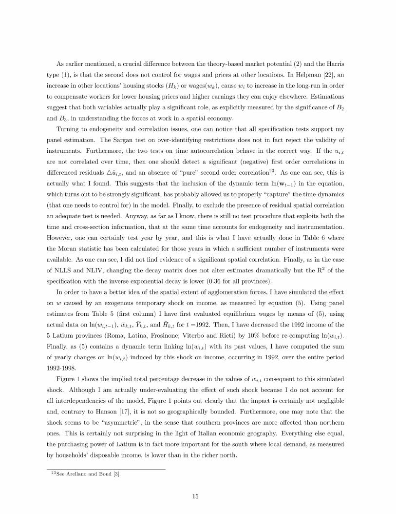
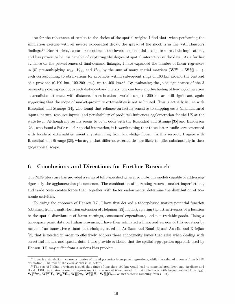
In order to have a better idea of the spatial extent of agglomeration forces, I have simulated the effect

on w caused by an exogenous temporary shock on income, as measured by equation (5). Using panel

estimates from Table 5 (first column) I have first evaluated equilibrium wages by means of (5), using

actual data on ln(wi,t−1), wk,t, Yk,t, and Hk,t for t =1992. Then, I have decreased the 1992 income of the

5 Latium provinces (Roma, Latina, Frosinone, Viterbo and Rieti) by 10% before re-computing ln(wi,t).

Finally, as (5) contains a dynamic term linking ln(wi,t) with its past values, I have computed the sum

of yearly changes on ln(wi,t) induced by this shock on income, occurring in 1992, over the entire period

1992-1998.

Figure 1 shows the implied total percentage decrease in the values of wi,t consequent to this simulated

shock. Although I am actually under-evaluating the effect of such shock because I do not account for

all interdependencies of the model, Figure 1 points out clearly that the impact is certainly not negligible

and, contrary to Hanson [17], it is not so geographically bounded. Furthermore, one may note that the

shock seems to be “asymmetric”, in the sense that southern provinces are more affected than northern

ones. This is certainly not surprising in the light of Italian economic geography. Everything else equal,

the purchasing power of Latium is in fact more important for the south where local demand, as measured

by households’ disposable income, is lower than in the richer north.

23 See Arellano and Bond [3].

15

As for the robustness of results to the choice of the spatial weights I find that, when performing the

simulation exercise with an inverse exponential decay, the spread of the shock is in line with Hanson’s

findings.24 Nevertheless, as earlier mentioned, the inverse exponential has quite unrealistic implications,

and has proven to be less capable of capturing the degree of spatial interaction in the data. As a further

evidence on the pervasiveness of final-demand linkages, I have expanded the number of linear regressors

in (5) pre-multiplying wk,t, Yk,t, and Hk,t by the sum of many spatial matrices (W1000 +W200

100 + ..),

each corresponding to observations for provinces within subsequent rings of 100 km around the centroid

of a province (0-100 km, 100-200 km.), up to 400 km.25 By evaluating the joint significance of the 3

parameters corresponding to each distance-band matrix, one can have another feeling of how agglomeration

externalities attenuate with distance. In estimations, variables up to 200 km are still significant, again

suggesting that the scope of market-proximity externalities is not so limited. This is actually in line with

Rosenthal and Strange [34], who found that reliance on factors sensitive to shipping costs (manufactured

inputs, natural resource inputs, and perishability of products) influences agglomeration for the US at the

state level. Although my results seems to be at odds with the Rosenthal and Strange [35] and Henderson

[23], who found a little role for spatial interaction, it is worth noting that these latter studies are concerned

with localized externalities essentially stemming from knowledge flows. In this respect, I agree with

Rosenthal and Strange [36], who argue that different externalities are likely to differ substantially in their

geographical scope.

6 Conclusions and Directions for Further Research

The NEG literature has provided a series of fully-specified general equilibrium models capable of addressing

rigorously the agglomeration phenomenon. The combination of increasing returns, market imperfections,

and trade costs creates forces that, together with factor endowments, determine the distribution of eco-

nomic activities.

Following the approach of Hanson [17], I have first derived a theory-based market potential function

(obtained from a multi-location extension of Helpman [22] model), relating the attractiveness of a location

to the spatial distribution of factor earnings, consumers’ expenditure, and non-tradable goods. Using a

time-space panel data on Italian provinces, I have then estimated a linearized version of this equation by

means of an innovative estimation technique, based on Arellano and Bond [3] and Anselin and Kelejian

[2], that is needed in order to effectively address those endogeneity issues that arise when dealing with

structural models and spatial data. I also provide evidence that the spatial aggregation approach used by

Hanson [17] may suffer from a serious bias problem.

24 In such a simulation, we use estimates of σ and µ coming from panel regressions, while the value of τ comes from NLIVestimation. The rest of the exercise works as before.25The size of Italian provinces is such that rings of less than 100 km would lead to some isolated locations. Arellano and

Bond (1991) estimator is used in regression, i.e. the model is estimated in first differences with lagged values of ln(wi,t),W100

0 wt,W1000 Yt,W100

0 Ht,W200100wt,W200

100Yt,W200100Ht,... as instruments (starting from t− 2).

16

My results are consistent with the hypothesis that final-demand linkages actually influence the distri-

bution of earnings. Furthermore, my simulations suggest that, contrary to Hanson [17], the scope of such

spatial externalities is not so limited. This latter result is mainly due to the different choice of the spatial

decay matrix. Nevertheless, I provide evidence in favor of the power function specification. As a further

check, I also perform some unstructured linear estimations using many distance-bands matrices in the

same spirit as Rosenthal and Strange [35] and Henderson [23]. Variables up to 200 km are found to be still

significant, further suggesting that attenuation of market-proximity externalities is less rapid compared to

other agglomeration forces.

There are several possible directions for further research. One natural extension of my framework would

be to obtain estimates using European data. As shown by Overman and Puga [30], national borders are

in fact less and less important in Europe, while regions are becoming the best unit of analysis. A second

issue is related to the simplifying assumptions that lead Helpman [22] to be cumbersome for empirical

interpretation. The fact that σ is at the same time a measure of different things in these kind of models

is annoying. A promising alternative approach is the one proposed by Ottaviano, Tabuchi, and Thisse

[29]. Using a more elaborated demand structure and transportation technology, this model allows in fact

a clear separation (by means of different parameters) of elasticity of demand, elasticity of substitution and

increasing returns, as well as firms’ pricing policies. Finally, a deeper understanding of the functional form

that is more suited to describe the degree of spatial interaction among data is needed. In this respect, the

pioneering work of Pinkse, Slade and Brett [31] that tries to endogenize the spatial correlation matrix by

means of polynomial approximation may turn out to be a useful tool.

References

[1] L. Anselin, Spatial Econometrics: Methods and Models, Kluwer Academic Publishers, Boston 1988.

[2] L. Anselin, H. H. Kelejian, Testing for spatial error autocorrelation in the presence of endogenousregressors,.International Regional Science Review 20 (1997) 153-182.

[3] M. Arellano, S. R. Bond, Some tests of Specification for panel data: Monte Carlo evidence and anapplication to employment equations, Review of Economic Studies 58 (1991) 277-297.

[4] S. Bentolila, J. J. Dolado, Labour Flexibility and Wages: Lessons from Spain Economic Policy 18(1994) 55-99.

[5] S. Bentolila, J. F. Jimeno, Regional Unemployment Persistence (Spain, 1976-1994), Labour Economics5 (1998) 25-51.

[6] D. Black, V. Henderson, A Theory of Urban Growth, Journal of Political Economy 107 (1999) 252-284.

[7] A. Ciccone, R. Hall, Productivity and the Density of Economic Activity, American Economic Review86 (1996) 54-70.

[8] P. P. Combes, M. Lafourcade, Transport Costs Decline and Regional Inequalities: Evidence fromFrance, CEPR Discussion Papers 2894 (2001).

[9] D. R. Davis, D. E. Weinstein, Market access, economic geography and comparative advantage: anempirical test, Journal of International Economics 59 (2003) 1-23.

17

[10] A. C. Disdiez, K. Head, Exaggerated Reports on the Death of Distance: Lessons from a Meta-Analysis,Mimeo, University of Paris I.

[11] B. Eichengreen, Labor markets and European monetary unification, in P. R. Masson, M. Taylor (Eds.),Policy issues in the operation of currency unions, Cambridge University Press, Cambridge, 1993, pp.130—162.

[12] R. C. Feenstra, New Product Varieties and the Measurement of International Prices, American Eco-nomic Review 84 (1994) 157-177.

[13] M. Fujita, P. Krugman, When in the Economy Monocentric? von Thunen and Chamberlin Unified,Regional Science and Urban Economics 25 (1995) 505-528.

[14] M. Fujita, J. F. Thisse, Economics of agglomeration, Journal of the japanese and internationaleconomies 10 (1996), 339-378.

[15] M. Fujita, P. Krugman, A. J. Venables, The spatial economy. Cities, regions and international trade,MIT Press, Cambridge 1999.

[16] M. Fujita, J. F. Thisse, Economics of Agglomeration, Cambridge University Press, Cambdridge 2002.

[17] G. H. Hanson, Market potential, increasing returns, and geographic concentration, NBER WorkingPaper 6429 (1998).

[18] G. H. Hanson, Scale Economies and the Geographic Concentration of Industry, Journal of EconomicGeography 1 (2001) 255-276.

[19] C. D. Harris, The Market as a Factor in the Localization of Industry in the United States, Annals ofthe Association of American Geographers 44 (1954) 315-348.

[20] K. Head, J. Ries, Increasing Returns Versus National Product Differentiation as an Explanation forthe Pattern of US-Canada Trade, American Economic Review.91 (2001) 858-876.

[21] K. Head, T. Mayer, Market Potential and the Location of Japanese Investment in the EuropeanUnion, CEPR Discussion paper 3455 (2002).

[22] E. Helpman, The Size of Regions, in D. Pines, E. Sadka, I. Zilcha (Eds.), Topics in Public Economics,Cambridge University Press, Cambridge 1998, pp. 33-54.

[23] J. V. Henderson, Marshall’s Scale Economies, Journal of Urban Economics 53 (2003) 1-28.

[24] J. V. Henderson, A. Kuncoro, M. Turner, Industrial Development and Cities, Journal of PoliticalEconomy 103 (1995) 1067-1081.

[25] P. Krugman, Increasing returns and economic geography, Journal of political economy 99 (1991)483-499.

[26] P. Krugman, Development, geography, and economic theory, MIT Press, Cambridge 1995.

[27] R. E. Lucas, On the mechanics of economic development, Journal of monetary economics 22 (1988)3-22.

[28] G. I. P. Ottaviano, D. Puga, Agglomeration in the global economy: A survey of the New EconomicGeography, The World Economy 21 (1998) 707-731.

[29] G. I. P. Ottaviano, T. Tabuchi, J. F. Thisse, Agglomeraion and Trade Revisited, International Eco-nomic Review 43 (2002) 409-436.

[30] H. G. Overman, D. Puga, Unemployment clusters across European regions and countries, EconomicPolicy 34 (2002) 115-147.

18

[31] J. Pinkse, M. E. Slade, C. Brett, Spatial Price Competition: A Semiparametric Approach, Economet-rica 70 (2002) 1111-1155.

[32] J. Roback, Wages, Rents, and the Quality of Life, Journal of Political Economy 90 (1982) 1257-1278.

[33] S. Rosen, Wage-Based Indexes of the Urban Quality of Life, in P. Mieszkowski, M. Straszheim (Eds.),Current Issues in Urban Economics, Johns Hopkins University Press, Baltimore 1979, 74-104.

[34] S. Rosenthal, W. Strange, The Determinants of Agglomeration, Journal of Urban Economics 50 (2001)191-229.

[35] S. Rosenthal, W. Strange, Geography, Industrial Organization, and Agglomeration, Review of Eco-nomics and Statistics 85 (2003) 377-393.

[36] S. Rosenthal, W. Strange, Evidence on the nature and sources of agglomeration economies, in V.Henderson, J. F. Thisse (Eds.), Handbook of Regional and Urban Economics, Vol. 4, North Holland,Amsterdam, 2004, forthcoming.

[37] A. C. F. Teixeira, Transport Policies in the Light of the New Economic Geography: The PortugueseExperience, Mimeo, CORE.

Appendix: Details of Estimations

To construct instruments for NLIV and regressors for NLLS, I have adopted the following procedure. I

first divide Italy into 11 zones using NUTS-1 regions. After having transformed (3) with a time difference,

for NLIV estimation I have then used, for each province, the change (over the time interval 1991-1998) in

the logarithm of the variables w, Y , and H of the corresponding zone (reconstructed aggregating provinces

data) as instruments. I thus have a set of exactly 3 instruments for the 3 parameters to estimate in (3),

and so there is no need of an optimal weighting matrix. For NLLS, I have instead used directly levels of w,

Y , and H, corresponding to the eleven zones, as regressors before making first difference and applying least

squares. In both cases, I have also neutralized,as in Hanson [17], the specific contribution of each province

in the formation of the corresponding zone aggregate variable. As a remedy for spatial heterogeneity, I have

used White heteroscedasticity-consistent standard errors. For the Moran test, I used the pseudo-regressors

as explanatory variables. Finally, all estimations have been performed with Gauss for Windows 3.2.38.

Panel estimates are two-step GMM ones and have been obtained with DPD 98 for Gauss. The model

is estimated in first differences, using past levels of all explanatory variables, from t − 2 and later, asinstruments. The reason why I treat all variables as endogenous is that, in unreported estimations, I

actually found evidence that also the housing stock process suffers from simultaneity. Estimations includes

time-dummies, while standard errors and tests are all heteroscedasticity consistent.

19

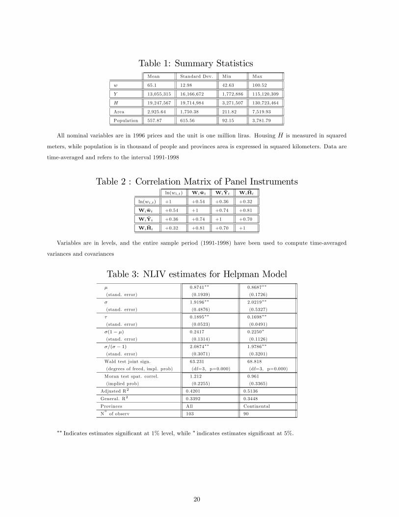
Table 1: Summary StatisticsMean Standard Dev. Min Max

w 65.1 12.98 42.63 100.52

Y 13,055,315 16,166,672 1,772,886 115,120,309

H 19,247,567 19,714,984 3,271,507 130,723,464

Area 2,925.64 1,750.38 211.82 7,519.93

Population 557.87 615.56 92.15 3,781.79

All nominal variables are in 1996 prices and the unit is one million liras. Housing H is measured in squared

meters, while population is in thousand of people and provinces area is expressed in squared kilometers. Data are

time-averaged and refers to the interval 1991-1998

Table 2 : Correlation Matrix of Panel Instrumentsln(wi,t) Wiwt WiYt WiHt

ln(wi,t) +1 +0.54 +0.36 +0.32

Wiwt +0.54 +1 +0.74 +0.81

WiYt +0.36 +0.74 +1 +0.70

WiHt +0.32 +0.81 +0.70 +1

Variables are in levels, and the entire sample period (1991-1998) have been used to compute time-averaged

variances and covariances

Table 3: NLIV estimates for Helpman Modelµ

(stand. error)

0.8741∗∗

(0.1939)

0.8687∗∗

(0.1726)

σ

(stand. error)

1.9196∗∗

(0.4876)

2.0219∗∗

(0.5327)

τ

(stand. error)

0.1895∗∗

(0.0523)

0.1698∗∗

(0.0491)

σ(1− µ)

(stand. error)

0.2417

(0.1314)

0.2250∗

(0.1126)

σ/(σ − 1)(stand. error)

2.0874∗∗

(0.3071)

1.9786∗∗

(0.3201)

Wald test joint sign.

(degrees of freed, impl. prob)

63.231

(df=3, p=0.000)

68.818

(df=3, p=0.000)

Moran test spat. correl.

(implied prob)

1.212

(0.2255)

0.961

(0.3365)

Adjusted R2 0.4201 0.5136

General. R2 0.3392 0.3448

Provinces All Continental

N◦of observ 103 90

∗∗ Indicates estimates significant at 1% level, while ∗ indicates estimates significant at 5%.

20

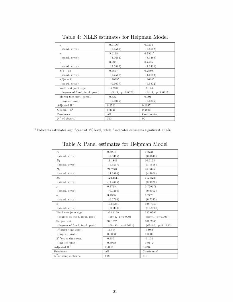
Table 4: NLLS estimates for Helpman Modelµ

(stand. error)

0.9106∗

(0.4561)

0.9394

(0.5652)

σ

(stand. error)

5.9128

(3.9692)

6.7531∗

(3.3469)

τ

(stand. error)

0.9351

(2.0882)

0.7495

(1.1421)

σ(1− µ)

(stand. error)

0.5877

(1.7527)

0.2880

(1.0182)

σ/(σ − 1)(stand. error)

1.2035∗

(0.6077)

1.2664∗

(0.5872)

Wald test joint sign.

(degrees of freed, impl. prob)

14.228

(df=3, p=0.0026)

15.124

(df=3, p=0.0017)

Moran test spat. correl.

(implied prob)

0.522

(0.6016)

0.991

(0.3216)

Adjusted R2 0.2521 0.1987

General. R2 0.2346 0.2893

Provinces All Continental

N◦of observ. 103 90

∗∗ Indicates estimates significant at 1% level, while ∗ indicates estimates significant at 5%.

Table 5: Panel estimates for Helpman ModelA

(stand. error)

0.3004

(0.0355)

0.2731

(0.0348)

B1

(stand. error)

11.1843

(1.5507)

10.9123

(1.7516)

B2

(stand. error)

27.7367

(4.2910)

28.3625

(4.5608)

B3

(stand. error)

122.4511

( 9.2635)

117.8225

(8.9225)

µ

(stand. error)

0.7735

(0.0316)

0.759278

(0.0302)

σ

(stand. error)

3.4335

(0.6796)

3.2778

(0.7345)

θ

(stand. error)

133.6351

(10.3401)

128.7353

(10.8708)

Wald test joint sign.

(degrees of freed, impl. prob)

333.1169

(df=4, p=0.000)

322.6295

(df=4, p=0.000)

Sargan test

(degrees of freed, impl. prob)

94.1325

(df=80, p=0.3621)

101.2946

(df=80, p=0.1953)

1storder time corr.

(implied prob)

-3.643

0.0003

-3.982

0.0000

2ndorder time corr.

(implied prob)

0.389

0.6972

-0.104

0.9172

Adjusted R2 0.4711 0.4568

Provinces All Continental

N◦of sample observ. 618 540

21

Table 6: Moran Test for panel estimations1993-1994 1994-1995 1995-1996 1996-1997 1997-1998

Moran test spat. correl. all provinces

(implied prob)

+0.2014

(0.8404)

+0.1301

(0.8965)

-0.7910

(0.4289)

-0.6370

(0.5241)

-0.4814

(0.6302)

Moran test spat. correl. cont. provinces

(implied prob)

+0.4114

(0.6808)

-0.5632

(0.5733)

-0.3120

(0.7550)

+0.1425

(0.8867)

-0.7123

(0.4763)

Test statistics have been computed with residuals of the model estimated in first differences.

% Change in w -0.07% to 0%

-0.1% to -0.07%

-0.2% to -0.1%

-0.5% to -0.2%

-1% to --0.5%

Figure 1: Simulated w changes from income shock to Latium

22