gimic documentation

gimic DocumentationRelease 0.0

GIMIC developers

Dec 03, 2021

Contents

1 Introduction 1

2 Installation 32.1 Parallelization . . . . . . . . . . . . . . . . . . . . . . . . . . . . . . . . . . . . . . . . . . . . . . 42.2 Installation on Stallo supercomputer . . . . . . . . . . . . . . . . . . . . . . . . . . . . . . . . . . . 42.3 Using BLAS1 and BLAS2 routines . . . . . . . . . . . . . . . . . . . . . . . . . . . . . . . . . . . 42.4 Installation on a Mac . . . . . . . . . . . . . . . . . . . . . . . . . . . . . . . . . . . . . . . . . . . 4

3 Testing 73.1 Adding new tests . . . . . . . . . . . . . . . . . . . . . . . . . . . . . . . . . . . . . . . . . . . . . 7

4 Important formulas 94.1 GIMIC key equation . . . . . . . . . . . . . . . . . . . . . . . . . . . . . . . . . . . . . . . . . . . 94.2 Anisotropy of the induced current (ACID) . . . . . . . . . . . . . . . . . . . . . . . . . . . . . . . . 9

5 Development 11

6 Usage 136.1 Interfaces to GIMIC . . . . . . . . . . . . . . . . . . . . . . . . . . . . . . . . . . . . . . . . . . . 13

7 The GIMIC input file 197.1 Keywords . . . . . . . . . . . . . . . . . . . . . . . . . . . . . . . . . . . . . . . . . . . . . . . . . 197.2 Grid section . . . . . . . . . . . . . . . . . . . . . . . . . . . . . . . . . . . . . . . . . . . . . . . 207.3 Advanced section . . . . . . . . . . . . . . . . . . . . . . . . . . . . . . . . . . . . . . . . . . . . . 217.4 Section: Essential . . . . . . . . . . . . . . . . . . . . . . . . . . . . . . . . . . . . . . . . . . . . 217.5 Current-density calculations . . . . . . . . . . . . . . . . . . . . . . . . . . . . . . . . . . . . . . . 227.6 Integration of the current strength . . . . . . . . . . . . . . . . . . . . . . . . . . . . . . . . . . . . 22

8 Grids 238.1 Basic grids . . . . . . . . . . . . . . . . . . . . . . . . . . . . . . . . . . . . . . . . . . . . . . . . 238.2 Bond grids . . . . . . . . . . . . . . . . . . . . . . . . . . . . . . . . . . . . . . . . . . . . . . . . 24

9 Description of generated files 27

10 Interactive bash scripts 2910.1 Introduction . . . . . . . . . . . . . . . . . . . . . . . . . . . . . . . . . . . . . . . . . . . . . . . 2910.2 Setup . . . . . . . . . . . . . . . . . . . . . . . . . . . . . . . . . . . . . . . . . . . . . . . . . . . 2910.3 Quick summary . . . . . . . . . . . . . . . . . . . . . . . . . . . . . . . . . . . . . . . . . . . . . 30

i

10.4 Detailed desctiption . . . . . . . . . . . . . . . . . . . . . . . . . . . . . . . . . . . . . . . . . . . 3010.5 Some tips and advice . . . . . . . . . . . . . . . . . . . . . . . . . . . . . . . . . . . . . . . . . . . 33

11 Vector plots 35

12 Streamlines 37

13 (Signed) modulus density plots 39

14 ACID plots 41

15 Interpretation of the results of GIMIC calculations 4315.1 3D integration . . . . . . . . . . . . . . . . . . . . . . . . . . . . . . . . . . . . . . . . . . . . . . 4315.2 Integration planes . . . . . . . . . . . . . . . . . . . . . . . . . . . . . . . . . . . . . . . . . . . . 45

ii

CHAPTER 1

Introduction

This is the GIMIC program for calculating magnetically induced currents in molecules. For this program produceany kind of useful information, you need to provide it with an AO density matrix and three (effective) magneticallyperturbed AO density matrices in the proper format. Currently only recent versions of ACES2 (CFOUR), Turbomole,QChem, LSDalton, FERMION++, Gaussian can produce these matrices. Dalton is in the works.If you would like toadd your favourite program to the list please use the source, Luke.

• For instructions how to compile and install this program refer to the INSTALL file in the top level directory.

• There is an annotated example input in the examples/ directory.

• For information on command line flags available run: ’gimic -help’

The following features have been implemented in the program

• Current densities in 2D or 3D

• The (signed) modulus of the current

• The divergence of the current (this is useful for checking gauge invariance vs. gauge independence). Note, thismodule does not work at the moment.

• Vector representation of the current in 2D or 3D

• Integration of the current flow through defined cut-planes in molecules

• Open-shells and spin currents

• Parallel execution through MPI (optional). Note, this works only if you check out the “stable” branch.

Utility programs to extract the AO density and perturbed densities from ACES2, Turbomole, QChem, LSDALTONand FERMION++ calculations are included in the GIMIC source distribution, see tools directory. Turbomole 5.10 andnewer also has the GIMIC interface built in.

1

gimic Documentation, Release 0.0

2 Chapter 1. Introduction

CHAPTER 2

Installation

Before compiling GIMIC you need to make sure that you have installed ideally all of the packages collected in therequirements.txt file. You need minimum the ones listed below.

* cython

* numpy

* runtest == 2.3.2

A convenient way to install the packages listed in requirements.txt is to install the Anaconda2 (https://www.anaconda.com/distribution/) Python distribution first. Then you can simply install all the packages listed in the filerequirements.txt by using:

$ conda install name-of-package

GIMIC requires CMake to configure and build. CMake is invoked via a front-end script called setup:

$ ./setup$ cd build$ make$ make install

To see all available options, run:

$ ./setup --help

Branch “master”:: GIMIC requires CMake to configure and build.:

$ mkdir build$ cd build$ cmake ../$ make$ make install

Test the installation with:

3

https://www.anaconda.com/distribution/

https://www.anaconda.com/distribution/


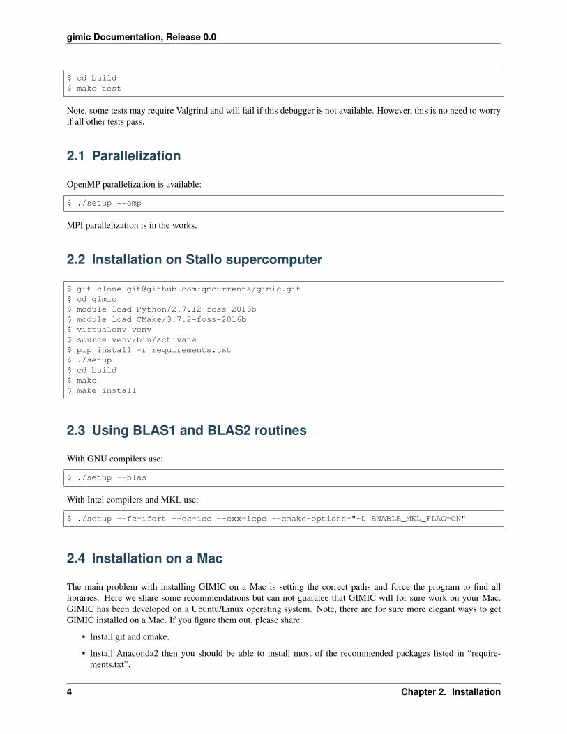
$ cd build$ make test

Note, some tests may require Valgrind and will fail if this debugger is not available. However, this is no need to worryif all other tests pass.

2.1 Parallelization

OpenMP parallelization is available:

$ ./setup --omp

MPI parallelization is in the works.

2.2 Installation on Stallo supercomputer

$ git clone [email protected]:qmcurrents/gimic.git$ cd gimic$ module load Python/2.7.12-foss-2016b$ module load CMake/3.7.2-foss-2016b$ virtualenv venv$ source venv/bin/activate$ pip install -r requirements.txt$ ./setup$ cd build$ make$ make install

2.3 Using BLAS1 and BLAS2 routines

With GNU compilers use:

$ ./setup --blas

With Intel compilers and MKL use:

$ ./setup --fc=ifort --cc=icc --cxx=icpc --cmake-options="-D ENABLE_MKL_FLAG=ON"

2.4 Installation on a Mac

The main problem with installing GIMIC on a Mac is setting the correct paths and force the program to find alllibraries. Here we share some recommendations but can not guaratee that GIMIC will for sure work on your Mac.GIMIC has been developed on a Ubuntu/Linux operating system. Note, there are for sure more elegant ways to getGIMIC installed on a Mac. If you figure them out, please share.

• Install git and cmake.

• Install Anaconda2 then you should be able to install most of the recommended packages listed in “require-ments.txt”.

4 Chapter 2. Installation


• For installing the C++ (gcc) and Fortran (gfortran) compilers you can use Xcode, Brew or MacPorts. You justneed to make sure that GIMIC is able to find them. A way to solve this is editing the “.bashrc” file.

• Check if you have the following paths in your “.bashrc”. If not add them.

– export PATH=/Users/your_username:/Users/your_username/anaconda/bin:$PATH

– PATH=”/Applications/CMake.app/Contents/bin”:”$PATH”

– export PATH=/Users/your_username/gimic/build/bin:$PATH

– export PATH=”/usr/local/bin:/usr/bin:/bin:/usr/sbin:/sbin”

2.4. Installation on a Mac 5


6 Chapter 2. Installation

CHAPTER 3

Testing

The testing procedure of the code is simplified using the runtest library written by Radovan Bast.

Make sure that you have it installed for the appropriate Python or virtual environment:

$ pip install git+https://github.com/bast/runtest.git@master

When compilation has completed, call make test from the build directory.

3.1 Adding new tests

Adding new tests can be done in the test directory. The provided tests can serve as example. The definition ofwhat are tested variables is done in the test executable. Remember to add the name of your new test in the test/CMakeLists.txt file. In case of doubts, read the documentation of runtest.

7

https://runtest.readthedocs.io


8 Chapter 3. Testing

CHAPTER 4

Important formulas

4.1 GIMIC key equation

The GIMIC working equation for the evaluation of the current density susceptibility tensor

$$ {\cal J}^{B_{\tau}}_{\gamma}(\mathbf{r}) = \sum_{\mu\nu} {D_{\mu\nu}}\frac{\partial\chi^*_\mu(\mathbf{r})}{\partial B_{\tau}} \frac{\partial h}{\partial m^K_{\gamma}}\chi_\nu(\mathbf{r}) + \sum_{\mu\nu} {D_{\mu\nu}} \chi^*_\mu(\mathbf{r}) \frac{\partialh}{\partial m^K_{\gamma}} \frac{\partial \chi_{\nu}(\mathbf{r})}{\partial B_{\tau}} + $$ $$\sum_{\mu\nu} \frac{\partial D_{\mu\nu} }{\partial B_{\tau}}\chi^*_{\mu}(\mathbf{r}) \frac{\partialh}{\partial m^K_{\gamma}}\chi_\nu(\mathbf{r}) -\epsilon_{\gamma\tau\delta} \big [ \sum_{\mu\nu}D_{\mu\nu}\chi^*_{\mu}(\mathbf{r}) \frac{\partial^2 h}{\partial m^K_{\gamma} \partial B_{\delta}}\chi_{\nu}(\mathbf{r})\big ] $$

See also:

1. J. Jusélius, D. Sundholm, J. Gauss, J. Chem. Phys., 121, 3952 (2004)

2. S. Taubert, D. Sundholm, J. Jus{‘e}lius, J. Chem. Phys., 134, 054132 (2011)

4.2 Anisotropy of the induced current (ACID)

The formula for the ACID method

$$ \Delta {\cal J}{^2}(\mathbf{r}) = \frac{1}{3} \big [ \big({\cal J}_x^x(\mathbf{r}) -{\cal J}_y^y(\mathbf{r})\big)^{2} + \big({\cal J}_y^y(\mathbf{r}) - {\cal J}_z^z(\mathbf{r})\big )^{2} + \big({\cal J}_z^z(\mathbf{r}) -{\cal J}_x^x(\mathbf{r})\big)^{2}\big] + $$ $$ \frac{1}{2} \big [ \big ( {\cal J}_x^y(\mathbf{r}) + {\calJ}_y^x(\mathbf{r})\big )^{2} + \big ( {\cal J}_x^z(\mathbf{r}) + {\cal J}_z^x(\mathbf{r}) \big )^{2} + \big ( {\calJ}_y^z(\mathbf{r}) + {\cal J}_z^y(\mathbf{r}) \big )^{2} \big ] $$

See also:

1. R. Herges and D. Geuenich, J. Phys. Chem. A, 105, 3214 (2001)

2. H. Fliegl, J. Jusélius and D. Sundholm, J. Phys. Chem. A, 120, 5658, (2016)

9


10 Chapter 4. Important formulas

CHAPTER 5

Development

The GIMIC code is based on Fortran and Python. Python is employed to parse the input files and call the Fortranexecutable (gimic.bin in the installation directory).

Remember to add tests using runtest for any new introduced features, as described in the Testing section of thedocumentation.

Adding new keywords to the GIMIC input file is done in the src/gimic.in file. The variable type is defined in thebeginning of the file. The keyword can be made compulsory or optional.

11


12 Chapter 5. Development

CHAPTER 6

Usage

Three files are needed in order to run GIMIC:

1. The XDENS file containing the effective one-particle density, and the magnetically perturbed densities in AObasis;

2. The MOL file with information on molecular geometry and basis sets;

3. The GIMIC input file. The default name is gimic.inp, however, any other file name is acceptable.

The XDENS and MOL files are obtained externally using other quantum chemistry programs which support an interfaceto gimic. Details are presented below.

Before doing the actual calculation with GIMIC, it might be a good idea to check if the grid is correctly defined. Thedryrun flag produces the grid.xyz file which can be examined in any molecular viewer.

$ gimic --dryrun

The calculation with GIMIC is started by:

$ gimic [gimic.inp] > gimic.out

The square brackets mean that it is not necessary to give the name of the input file if it is called gimic.inp since itis recognised by default.

6.1 Interfaces to GIMIC

The following sections explains how to obtain the XDENS and the MOL files.

6.1.1 Running TURBOMOLE

As of TURBOMOLE 5.10, the GIMIC interface is part of the official distribution. To produce the necessary files to runGIMIC, you first need to optimize the wavefunction/density of the molecule, before running the mpshift programwhich produces the perturbed density matrices. Before you run mpshift, you need to edit the control file and

13


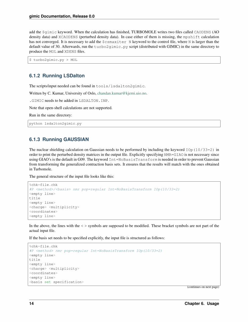
add the $gimic keyword. When the calculation has finished, TURBOMOLE writes two files called CAODENS (AOdensity data) and XCAODENS (perturbed density data). In case either of them is missing, the mpshift calculationhas not converged. It is necessary to add the $csmaxiter N keyword to the control file, where N is larger than thedefault value of 30. Afterwards, run the turbo2gimic.py script (distributed with GIMIC) in the same directory toproduce the MOL and XDENS files.

$ turbo2gimic.py > MOL

6.1.2 Running LSDalton

The scripts/input needed can be found in tools/lsdalton2gimic.

Written by C. Kumar, University of Oslo, [email protected].

.GIMIC needs to be added in LSDALTON.INP.

Note that open-shell calculations are not supported.

Run in the same directory:

python lsdalton2gimic.py

6.1.3 Running GAUSSIAN

The nuclear shielding calculation on Gaussian needs to be performed by including the keyword IOp(10/33=2) inorder to print the perturbed density matrices in the output file. Explicitly specifying NMR=GIAO is not necessary sinceusing GIAO’s is the default in G09. The keyword Int=NoBasisTransform is needed in order to prevent Gaussianfrom transforming the generalized contraction basis sets. It ensures that the results will match with the ones obtainedin Turbomole.

The general structure of the input file looks like this:

%chk=file.chk#P <method>/<basis> nmr pop=regular Int=NoBasisTransform IOp(10/33=2)<empty line>title<empty line><charge> <multiplicity><coordinates><empty line>

In the above, the lines with the < > symbols are supposed to be modified. These bracket symbols are not part of theactual input file.

If the basis set needs to be specified explicitly, the input file is structured as follows:

%chk=file.chk#P <method> nmr pop=regular Int=NoBasisTransform IOp(10/33=2)<empty line>title<empty line><charge> <multiplicity><coordinates><empty line><basis set specification>

(continues on next page)

14 Chapter 6. Usage

mailto:[email protected]


(continued from previous page)

<****><empty line>

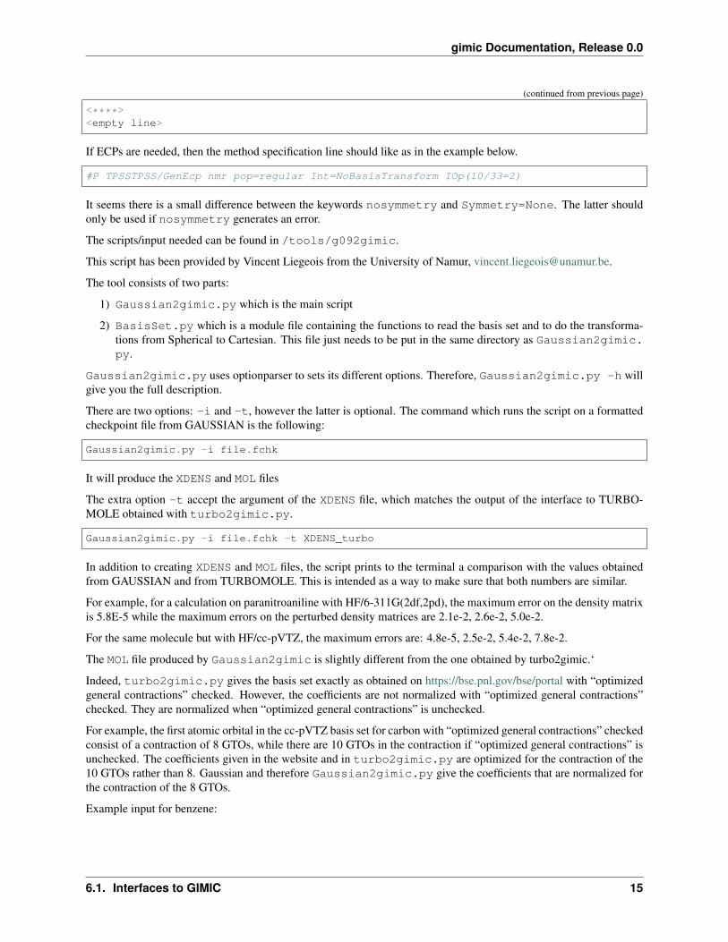
If ECPs are needed, then the method specification line should like as in the example below.

#P TPSSTPSS/GenEcp nmr pop=regular Int=NoBasisTransform IOp(10/33=2)

It seems there is a small difference between the keywords nosymmetry and Symmetry=None. The latter shouldonly be used if nosymmetry generates an error.

The scripts/input needed can be found in /tools/g092gimic.

This script has been provided by Vincent Liegeois from the University of Namur, [email protected].

The tool consists of two parts:

1) Gaussian2gimic.py which is the main script

2) BasisSet.py which is a module file containing the functions to read the basis set and to do the transforma-tions from Spherical to Cartesian. This file just needs to be put in the same directory as Gaussian2gimic.py.

Gaussian2gimic.py uses optionparser to sets its different options. Therefore, Gaussian2gimic.py -h willgive you the full description.

There are two options: -i and -t, however the latter is optional. The command which runs the script on a formattedcheckpoint file from GAUSSIAN is the following:

Gaussian2gimic.py -i file.fchk

It will produce the XDENS and MOL files

The extra option -t accept the argument of the XDENS file, which matches the output of the interface to TURBO-MOLE obtained with turbo2gimic.py.

Gaussian2gimic.py -i file.fchk -t XDENS_turbo

In addition to creating XDENS and MOL files, the script prints to the terminal a comparison with the values obtainedfrom GAUSSIAN and from TURBOMOLE. This is intended as a way to make sure that both numbers are similar.

For example, for a calculation on paranitroaniline with HF/6-311G(2df,2pd), the maximum error on the density matrixis 5.8E-5 while the maximum errors on the perturbed density matrices are 2.1e-2, 2.6e-2, 5.0e-2.

For the same molecule but with HF/cc-pVTZ, the maximum errors are: 4.8e-5, 2.5e-2, 5.4e-2, 7.8e-2.

The MOL file produced by Gaussian2gimic is slightly different from the one obtained by turbo2gimic.‘

Indeed, turbo2gimic.py gives the basis set exactly as obtained on https://bse.pnl.gov/bse/portal with “optimizedgeneral contractions” checked. However, the coefficients are not normalized with “optimized general contractions”checked. They are normalized when “optimized general contractions” is unchecked.

For example, the first atomic orbital in the cc-pVTZ basis set for carbon with “optimized general contractions” checkedconsist of a contraction of 8 GTOs, while there are 10 GTOs in the contraction if “optimized general contractions” isunchecked. The coefficients given in the website and in turbo2gimic.py are optimized for the contraction of the10 GTOs rather than 8. Gaussian and therefore Gaussian2gimic.py give the coefficients that are normalized forthe contraction of the 8 GTOs.

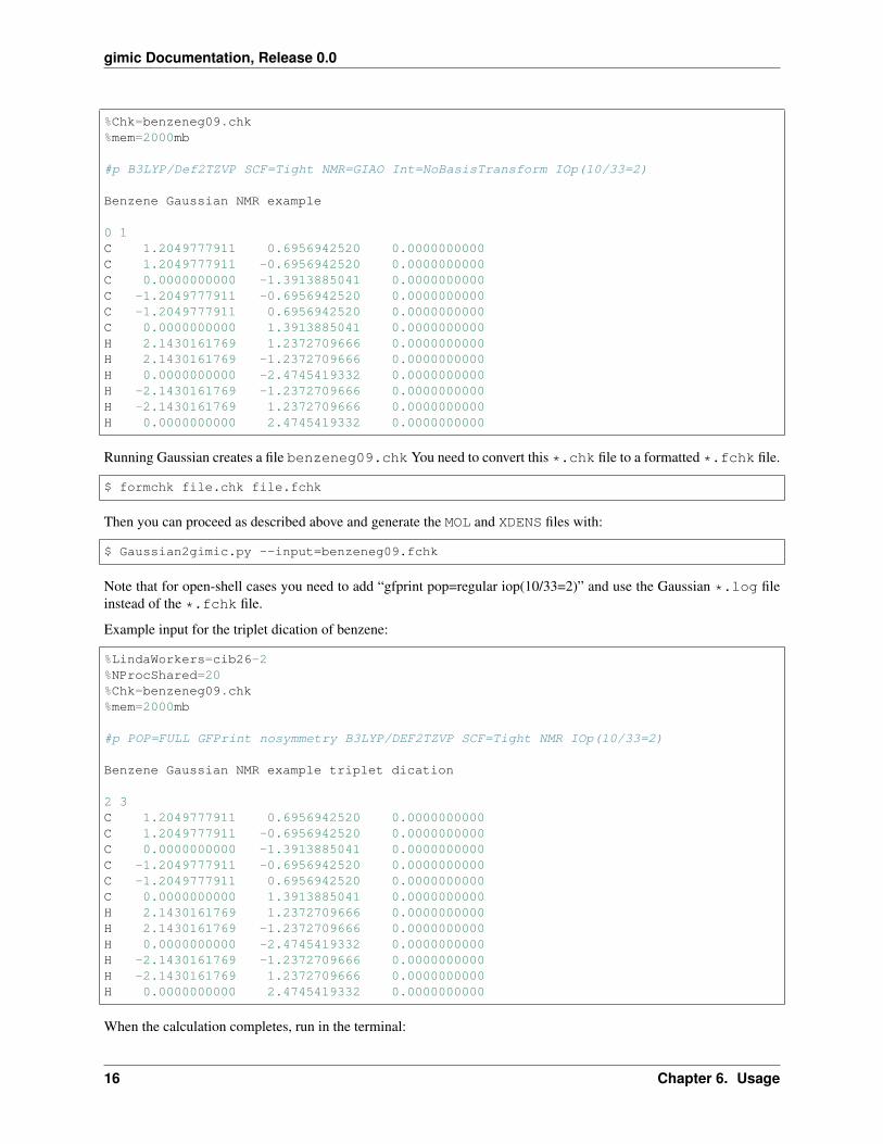
Example input for benzene:

6.1. Interfaces to GIMIC 15


https://bse.pnl.gov/bse/portal


%Chk=benzeneg09.chk%mem=2000mb

#p B3LYP/Def2TZVP SCF=Tight NMR=GIAO Int=NoBasisTransform IOp(10/33=2)

Benzene Gaussian NMR example

0 1C 1.2049777911 0.6956942520 0.0000000000C 1.2049777911 -0.6956942520 0.0000000000C 0.0000000000 -1.3913885041 0.0000000000C -1.2049777911 -0.6956942520 0.0000000000C -1.2049777911 0.6956942520 0.0000000000C 0.0000000000 1.3913885041 0.0000000000H 2.1430161769 1.2372709666 0.0000000000H 2.1430161769 -1.2372709666 0.0000000000H 0.0000000000 -2.4745419332 0.0000000000H -2.1430161769 -1.2372709666 0.0000000000H -2.1430161769 1.2372709666 0.0000000000H 0.0000000000 2.4745419332 0.0000000000

Running Gaussian creates a file benzeneg09.chk You need to convert this *.chk file to a formatted *.fchk file.

$ formchk file.chk file.fchk

Then you can proceed as described above and generate the MOL and XDENS files with:

$ Gaussian2gimic.py --input=benzeneg09.fchk

Note that for open-shell cases you need to add “gfprint pop=regular iop(10/33=2)” and use the Gaussian *.log fileinstead of the *.fchk file.

Example input for the triplet dication of benzene:

%LindaWorkers=cib26-2%NProcShared=20%Chk=benzeneg09.chk%mem=2000mb

#p POP=FULL GFPrint nosymmetry B3LYP/DEF2TZVP SCF=Tight NMR IOp(10/33=2)

Benzene Gaussian NMR example triplet dication

2 3C 1.2049777911 0.6956942520 0.0000000000C 1.2049777911 -0.6956942520 0.0000000000C 0.0000000000 -1.3913885041 0.0000000000C -1.2049777911 -0.6956942520 0.0000000000C -1.2049777911 0.6956942520 0.0000000000C 0.0000000000 1.3913885041 0.0000000000H 2.1430161769 1.2372709666 0.0000000000H 2.1430161769 -1.2372709666 0.0000000000H 0.0000000000 -2.4745419332 0.0000000000H -2.1430161769 -1.2372709666 0.0000000000H -2.1430161769 1.2372709666 0.0000000000H 0.0000000000 2.4745419332 0.0000000000

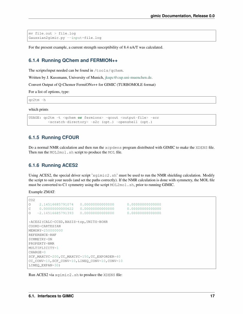
When the calculation completes, run in the terminal:

16 Chapter 6. Usage


mv file.out > file.logGaussian2gimic.py --input=file.log

For the present example, a current strength susceptibility of 8.4 nA/T was calculated.

6.1.4 Running QChem and FERMION++

The scripts/input needed can be found in /tools/qchem.

Written by J. Kussmann, University of Munich, [email protected].

Convert Output of Q-Chemor FermiONs++ for GIMIC (TURBOMOLE format)

For a list of options, type:

qc2tm -h

which prints

USAGE: qc2tm -t <qchem or fermions> -qcout <output-file> -scr<scratch-directory> -s2c (opt.) -openshell (opt.)

6.1.5 Running CFOUR

Do a normal NMR calculation and then run the xcpdens program distributed with GIMIC to make the XDENS file.Then run the MOL2mol.sh script to produce the MOL file.

6.1.6 Running ACES2

Using ACES2, the special driver script ’xgimic2.sh’ must be used to run the NMR shielding calculation. Modifythe script to suit your needs (and set the paths correctly). If the NMR calculation is done with symmetry, the MOL filemust be converted to C1 symmetry using the script MOL2mol.sh, prior to running GIMIC.

Example ZMAT:

CO2O 2.14516685791074 0.00000000000000 0.00000000000000C 0.00000000000622 0.00000000000000 0.00000000000000O -2.14516685791393 0.00000000000000 0.00000000000000

*ACES2(CALC=CCSD,BASIS=tzp,UNITS=BOHRCOORD=CARTESIANMEMORY=250000000REFERENCE=RHFSYMMETRY=ONPROPERTY=NMRMULTIPLICITY=1CHARGE=0SCF_MAXCYC=200,CC_MAXCYC=150,CC_EXPORDER=40CC_CONV=10,SCF_CONV=10,LINEQ_CONV=10,CONV=10LINEQ_EXPAN=30)

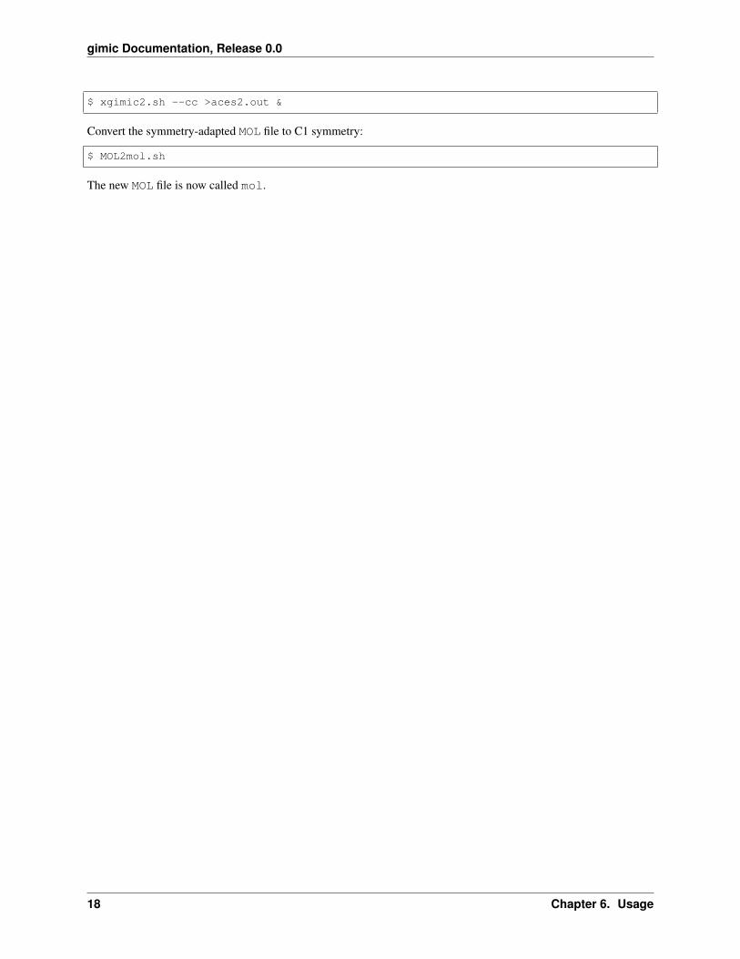
Run ACES2 via xgimic2.sh to produce the XDENS file:

6.1. Interfaces to GIMIC 17



$ xgimic2.sh --cc >aces2.out &

Convert the symmetry-adapted MOL file to C1 symmetry:

$ MOL2mol.sh

The new MOL file is now called mol.

18 Chapter 6. Usage

CHAPTER 7

The GIMIC input file

The GIMIC input file is parsed by the getkw python parser, which defines a grammar system based on sectionsand keywords in a recursive manner. The input is in principle line oriented, but lines may be continued using a pipesymbol | at the end of a line. Furthermore, blanks and tabs are insignificant, with the exception of strings. Lines maybe commented until end-of-line with a hash sign (#).

Sections are delimited by curly brackets section{...}, and may have a keyword argument enclosed in parenthesessection(argument){...}.

Keywords come in two different types; simple keywords consisting of integers, reals or strings (enclosed in doublequote marks "string"), and array keywords. Array keywords are enclosed in square brackets and the elements –integers, reals or strings – are delimited by a comma, e.g. keyword = [0,1,2].

7.1 Keywords

The top level section defines a few global parameters:

calc=cdens,integral This keyword determines what is to be calculated, and in what order. The possible options are:’cdens’ – calculate current densities, ’integral’ – integrate the current flow through a cut-plane. Each of theseoptions have their own respective sections to specify options and grids.

title Useless keyword, but since every program with a bit of self respect has a title, GIMIC also has one. . .

basis=MOL Name of the MOL file (eg. MOL or mol or whatever). A relative path can also be given.

density=XDENS Name of the density file (eg. XDENS). A relative path can also be given.

debug=1 Set debug level. The higher the number, the more useless output one gets.

openshell=false Open-shell calculation

magnet=[Bx,By,Bz] Define the direction of the external magnetic field by its vector components

magnet_axis=z Specify the magnetic field along a defined axis. Valid options are: i,j,k or x,y,z or X. “i,j,k” are thedirections of the basis vectors defining the integration plane. “x,y,z” are the absolute fixed laboratory axis. Notethat magnet\_axis=X is used to specify the magnetic field along the direction which is orthogonal to themolecular plane, but parallel to the integration plane.

19


7.2 Grid section

7.2.1 Grid types

The currently implemented grids are

even The grid points are spaced uniformly

base Uniformly distributed grid points in 2D or 3D. Used in current-density calculations

bond Defining an integration plane passing through a particular chemical bond. Used for the integration of the currentstrength.

Custom grids can also be employed.

7.2.2 Definition

A grid can be defined in the following manner:

Grid(type) { . . .

}

7.2.3 Bond grid

The keywords specific to the bond type grid employed in the integration of the strength of the current density are:

bond=[a,b] Define the integration plane to cross the bond betweens atoms a and b. The indices are chosen accordingto the MOL file (coord file from Turbomole calculations). Alternatively, two Cartesian coordinates can beemployed via the keywords coord1 and coord2.

coord1 = [x1,y1,z1] and

coord2 = [x2,y2,z2] Specify a pair of Cartesian coordinates instead of atomic indices. The integration plane will crossthe line between the two points. Alternatively, use atomic indices using the keyword bond=[a,b].

fixpoint=c Specify an atomic index to use as the third point defining the integration plane. Alternatively, specify anarbitrary point using the keyword fixcoord.

fixcoord=[x, y, z] Specify an arbitrary point in 3D as the third point defining the integration plane. Alternatively,specify an atomic index using the keyword fixpoint.

distance=r Define the distance between the two atoms or two Cartesian coordinates between which the integrationplane will cross.

height=[-a, b] Specify the distance a between the bottom vertex of the integration plane and the bond using thenumber -a. Specify the distance b between the top vertex of the integration plane and the bond using the numberb.

width=[-a,b] Specify the lengths a and b on both sides of the chemical bond.

type=gauss Use Gauss distribution of grid points for the Gauss quadrature

gauss_order=9 The order of the Gauss quadrature

20 Chapter 7. The GIMIC input file


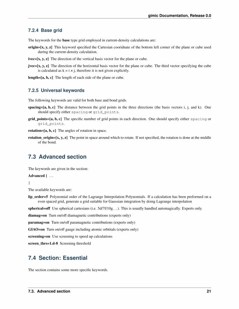
7.2.4 Base grid

The keywords for the base type grid employed in current-density calculations are:

origin=[x, y, z] This keyword specified the Cartesian cooridnate of the bottom left corner of the plane or cube usedduring the current-density calculation.

ivec=[x, y, z] The direction of the vertical basis vector for the plane or cube.

jvec=[x, y, z] The direction of the horizontal basis vector for the plane or cube. The third vector specifying the cubeis calculated as k = i × j, therefore it is not given explicitly.

length=[a, b, c] The length of each side of the plane or cube.

7.2.5 Universal keywords

The following keywords are valid for both base and bond grids.

spacing=[a, b, c] The distance between the grid points in the three directions (the basis vectors i, j, and k). Oneshould specify either spacing or grid_points.

grid_points=[a, b, c] The specific number of grid points in each direction. One should specify either spacing orgrid_points.

rotation=[a, b, c] The angles of rotation in space.

rotation_origin=[x, y, z] The point in space around which to rotate. If not specified, the rotation is done at the middleof the bond.

7.3 Advanced section

The keywords are given in the section:

Advanced { . . .

}

The available keywords are:

lip_order=5 Polynomial order of the Lagrange Interpolation Polynomials. If a calculation has been preformed on aeven spaced grid, generate a grid suitable for Gaussian integration by doing Lagrange interpolation

spherical=off Use spherical cartesians (i.e. 5d/7f/10g. . . ). This is usually handled automagically. Experts only.

diamag=on Turn on/off diamagnetic contributions (experts only)

paramag=on Turn on/off paramagnetic contributions (experts only)

GIAO=on Turn on/off gauge including atomic orbtitals (experts only)

screening=on Use screening to speed up calculations

screen_thrs=1.d-8 Screening threshold

7.4 Section: Essential

The section contains some more specific keywords.

7.3. Advanced section 21


7.4.1 ACID calculations

ACID calculations can be defined by setting the calculation type to calc=cdens and the grid to type base:Grid(base) {...}

acid=on Turn on/off ACID calculation. It can only be done in current-density calculations with the calc=cdenskeyword and the respective grid.

7.4.2 Modulus of the current density

Calculate the mod(J) integral, this is useful to verify that the actual integration grid is sensible in “tricky” molecules.

jmod=off Unless necessary, it should be turned off to save computational time.

7.5 Current-density calculations

Current density calculations are specified using the keyword calc = cdens.

ACID calculations can be performed in the current-density cal

acid=on Turn on/off ACID calculation

The produced files can be visualised in ParaView:

• acid.vti: contains information about ACID function as VTK file compatible with ParaView

• jvec.vti: contains information about the current density vector function as VTK file compatible with Par-aView

• jmod.vti: contains the signed modulus of the current density vector function and can be visualized via twoisosurfaces in ParaView

Calculate the mod(J) integral, this is useful to verify that the actual integration grid is sensible in “tricky” molecules.

7.6 Integration of the current strength

The calculation type has to be set to calc=integral and the grid to type bond. Grid(bond) {...}

22 Chapter 7. The GIMIC input file

CHAPTER 8

Grids

There are three possible grid topologies in gimic: ‘std (or base)’ which is 3-dimensional (although the extend in onedirection may be zero), ‘bond’ which is 2-dimensional, and ‘file’ which is an arbitrary set of points read from a file.‘std’ grids are especially useful for visualisations of an entire current vector field. ‘bond’ grid are used to integrate thecurrent that flows through the grid.

For an ‘std’ or ‘bond’ grid one can specify the spacing (type) of points in each dimension. The choices are ‘even’ foran equidistant grid, ‘gauss’ for a Gauss grid and ‘lobatto’ for a Gauss-Lobatto grid. The recommended choices are‘even’ for ‘std’ and ‘gauss’ for ‘bond’. When a quadrature grid is specified the order of the quadrature must also bespecified with the ’gauss_order’ keyword. The number of grid points in each direction is specified either explicitlyusing either of the array keywords ’grid_points’ or ’spacing’. If the chosen grid is not a simple even spaced grid, theactual number of grid points will be adjusted upwards to fit the requirements of the chosen quadrature.

The shape of the grid can also be modified by the ’radius’ key, which specifies a cutoff radius. This can be useful forintegration. Sometimes it’s practical to be able to specify a grid relative to a well know starting point. The ’rotation’keyword specifies Euler angles for rotation according to the x->y->z convention. Note that the magnetic field is notrotated, unless it is specified with ’magnet_axis=i,j or k’.

GIMIC automatically outputs a number of .xyz files containing dummy points to show how the grids defined actuallyare laid out in space.

8.1 Basic grids

The ’std’ grid is defined by giving an ’origin’ and two orthogonal basis vectors ’ivec’ and ’jvec’ which define a plane.The third axis is determined from =×�⃗�.𝑇ℎ𝑒𝑎𝑟𝑟𝑎𝑦′𝑙𝑒𝑛𝑔𝑡ℎ𝑠′𝑠𝑝𝑒𝑐𝑖𝑓𝑖𝑒𝑠𝑡ℎ𝑒𝑔𝑟𝑖𝑑𝑑𝑖𝑚𝑒𝑛𝑠𝑖𝑜𝑛𝑠𝑖𝑛𝑒𝑎𝑐ℎ𝑑𝑖𝑟𝑒𝑐𝑡𝑖𝑜𝑛.

8.1.1 grid(std)

type=evenorigin=-8.0, -8.0, 0.0

Origin of grid


23



ivec=1.0, 0.0, 0.0Basis vector i

jvec=0.0, 1.0, 0.0Basis vector j ( k = i x j )

lengths=16.0, 16.0, 0.0Lenthts of (i,j,k)

spacing=0.5, 0.5, 0.5Spacing of points on grid (i,j,k)

grid\_points=50, 50, 0Number of gridpoints on grid (i,j,k)

rotation=0.0, 0.0, 0.0Rotation of (i,j,k) -> (i’,j’,k’) in degrees. Given as Euler anglesin the x->y->z convention.

8.2 Bond grids

The ’bond’ type grids define a plane through a bond, or any other defined vector. The plane is orthogonal to the vectordefining the bond. The bond can be specified either by giving two atom indices, ’bond=[1,2]’, or by specifying a pairof coordinates, ’coord1’ and ’coord2’. The position of the grid between two atoms is determined by the ’distance’key, which specifies the distance from atom 1 towards atom 2. For analysing dia- and paramagnetic contributions, thepositive direction of the bond is taken to be from atom 1 towards atom 2. Since one vector is not enough to uniquelydefining the coordinate system (rotations around the bond are arbitrary), a fixpoint must be specified using either the’fixpoint’ atom index or the ’fixcoord’ keyword. This triple of coordinates is also used to fix the direction of themagnetic field when the ’magnet_axis=T’ is used.

The shape and size of the bond grid is specified by the keywords ‘width’ and ‘height’. Each of the four components isrelative to a point on the line connecting the two reference atoms/coordinates. Typically (but not necessarily) the firstcomponent of both ranges is negative and the second component is positive.

width=[-1.5, 5.0]height=[-5.0, 5.0]

8.2.1 grid(bond):

type=gauss|lobatto Use uneven distribution of grid points for quadrature

bond=1,2 Atom indices for bond specification

fixpoint=5 Atom index to use for fixing the magnetic field and grid orientation

coord1=0.0, 0.0, 3.14 Coordinate of atom 1

coord2=0.0, 0.0, -3.14 Coordinate of atom 2

fixcoord=0.0, 0.0, 0.0 Fixation coordinate

distance=1.5 Place grid ’distance’ between atoms 1 and atom 2

gauss_order=9 Order for Gauss quadrature

24 Chapter 8. Grids


spacing=0.5, 0.5, 0.5 Spacing of points on grid (i,j,k) (approximate)

grid_points=50, 50, 0 Number of grid points on grid (i,j,k) (approximate)

height=-4.0, 4.0 Grid size relative to grid center

width=-1.0, 6.0 Grid size relative to grid center

radius=3.0 Create a round grid by cutting off at radius

rotation=0.0, 0.0, 0.0 Rotation of (i,j,k) -> (i’,j’,k’) in degrees. Given as Euler angles in the x->y->z convention.

8.2. Bond grids 25


26 Chapter 8. Grids

CHAPTER 9

Description of generated files

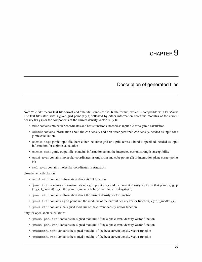
Note “file.txt” means text file format and “file.vti” stands for VTK file format, which is compatible with ParaView.The text files start with a given grid point (x,y,z) followed by either information about the modulus of the currentdensity f(x,y,z) or the components of the current density vector Jx,Jy,Jz.

• MOL: contains molecular coordinates and basis functions, needed as input file for a gimic calculation

• XDENS: contains information about the AO density and first order perturbed AO density, needed as input for agimic calculation

• gimic.inp: gimic input file, here either the cubic grid or a grid across a bond is specified, needed as inputinformation for a gimic calculation

• gimic.out: gimic output file, contains information about the integrated current strength susceptibility

• grid.xyz: contains molecular coordinates in Ångstrøm and cube points (8) or integration plane corner points(4)

• mol.xyz: contains molecular coordinates in Ångstrøm

closed-shell calculation:

• acid.vti: contains information about ACID function

• jvec.txt: contains information about a grid point x,y,z and the current density vector in that point jx, jy, jz(x,y,z, f_current(x,y,z), the point is given in bohr (it used to be in Ångstrøm)

• jvec.vti: contains information about the current density vector function

• jmod.txt: contains a grid point and the modulus of the current density vector function, x,y,z, f_mod(x,y,z)

• jmod.vti: contains the signed modulus of the current density vector function

only for open-shell calculations:

• jmodalpha.txt: contains the signed modulus of the alpha current density vector function

• jmodalpha.vti: contains the signed modulus of the alpha current density vector function

• jmodbeta.txt: contains the signed modulus of the beta current density vector function

• jmodbeta.vti: contains the signed modulus of the beta current density vector function

27


• jmodspindens.txt: contains the signed modulus of the difference (alpha - beta) current density vectorfunction

• jmodspindens.vti: contains the signed modulus of the difference (alpha - beta) current density vectorfunction

• jvecalpha.txt: contains information about the alpha current density vector function

• jvecalpha.vti: contains information about the alpha current density vector function

• jvecbeta.txt: contains information about the beta current density vector function

• jvecbeta.vti: contains information about the beta current density vector function

• jvecspindens.txt: contains information about the difference (alpha - beta) current density vector function

• jvecspindens.vti: contains information about the difference (alpha - beta) current density vector function

28 Chapter 9. Description of generated files

CHAPTER 10

Interactive bash scripts

10.1 Introduction

GIMIC calculations can be started interactively using bash scripts. They are useful for adjusting the integrationplane of choice, for starting current profile analysis, and submission of parallel tasks on a cluster with the SLURMschedulilng system (i.e. one where you submit jobs using sbatch. There is a local version for the current profileanalysis, which can run on a laptop, for example. Note that at the moment they are working with the coord file fromTURBOMOLE. It will not be hard to make the input universal by using an XYZ file instead, so if you need it, let usknow. The current density analyses employing GIMIC are most easily done if the magnetic field, pointing along the Zaxis, is perpendicular to the molecular plane of a planar molecule. The orientation of the magnetic field can, of course,be modified accordingly.

NOTE: The script assumes that the MOL and XDENS files exist. They can prepared using turbo2gimic.py orGaussian2gimic.py once the nuclear shielding calculation has finished. Also the coordinates need to be preparedin XYZ format, too. This can be done with the Turbomole script for conversion of the coord file to XYZ format.

t2x coord > coord.xyz

10.2 Setup

In the jobscripts directory there is a script called setup.sh. It takes care of preparing the scripts for the specificmachine.

NOTE: When preparing the scripts for a cluster, first it is necessary to modify the jobscript-header file beforerunning setup.sh. You likely need to adjust the name of the partition, number of tasks per node according to thespecific cluster, as well as load the necessary modules in order to start GIMIC. Do not add time limit, job task name,or number of cores as parameters because the GIMIC script will ask for that before submitting the calculation.

Remember, that the setup script hardcodes the paths to the directories, so if you want to use the scripts on anothercomputer, you need to execute ./setup there. Setup needs to be done only once - after you git pull, so as toinstall the newly implemented features and bug fixes. The prepared scripts can then be called from the calculation

29


directory. should be called. The workflow can be made easier by add the export $GIMIC_HOME=/your/own/path, which is printed after setup. There are some bash aliases and functions in the file useful-aliases, whichyou may want to add to your ./bashrc.

The scripts are still under development but the ones that are recommended for use at the moment arecurrent-profile-cluster.sh, current-profile-local.sh, and gimic-run.sh. The others arestill in development phase, so if you are curious, you can try but functionality might be unclear or limited.

VMD is a highly-recommended tools for visualisation of molecules, in particular, the integration planes.

10.3 Quick summary

1. Choose an integration plane

2. If not obvious where to start integrating from, you can test its beginning and end points using the gimic-run.sh script and visualise the grid.xyz file. Adjust the gimic.inp file manually if necessary.

3. Run the current profile for the integration plane (current-profile-local.sh if running on your laptop,or current-profile-cluster.sh if submitting as batch job on a cluster).

4. Inspect the profile plot, check the sign of the currents, reverse the signs if necessary.

5. Make a better-quality plot using the plot-current-profile.sh script.

10.4 Detailed desctiption

In the jobscripts directory you can find several bash scripts. They should be called as:

EXAMPLE:

$ $GIMIC_HOME/jobscripts/current-profile-cluster.sh

# OR if using the suggested aliases:

$ gcurrent

The input for the scripts is based on selecting two atoms between which the integration plane lies. By default theintegration plane is perpendicular to the bond between them. When you start the script, it asks for indices of theselected atoms according to the coord file. The atomic indices should be given in counter-clockwise manner. Wehave a sign problem, so for now we have to live with the fact that sometimes the diatropic current and the paratropiccurrent can have the wrong sign but the magnitude is obtained correctly. Meaning that it is not necessary to restartthe calculation if the signs are inverted. It can be post-processed. In planar molecules the choice of the two atoms isstraight-forward but in non-planar ones, you need to choose the two atoms to be with very similar Z coordinates whenplacing the magnetic field in the Z direction. It is a known issue, which will hopefully be resolved in the future.

TIP: Check the indices of the atoms from the xyz file, for example with xmakemol.

NOTE: Atom indices start from 0 in VMD, whereas in GIMIC and xmakemol, they start from 1.

A directory with a name include the atomic indices of the bond is created, for example current_profile_39.119. This means that several current profiles can be analysed at the same time, each written to a directory of its own.If a directory with the same calculation already exists, it will ask for confirmation to overwrite it.

Next, you need to define the dimensions of the integration plane. It crosses the bond at the midpoint between the twoattoms by default, however if needed, one can shift it to be closer to the one or the other atom. Usually we are interestedin starting the integration from the centre of a ring to infinity, or maybe from the centre of the ring to another. Twoparameters take care of that: the start value and the out value. These parameters can be defined either by manually

30 Chapter 10. Interactive bash scripts


entering a distance in atomic units, or using the atomic indices as defined in the coord file. By default, the scriptoffers integration to infinity, which for practical purposes means 10 bohr. When entering these atomic indices, pleasetype them on the same row and then press enter, for example,

1 2 3 4 5 [ENTER]

TIP: The integration can be defined to start or end at the centre of any number of atoms, including single atoms.

The script will calculate the distance between the bond and the geometric centre of the selected atoms. It is rec-ommended to add extra 0.5 bohr because the origin of the vortex lies in the geometrical centre of the ring only forsymmetric molecules. Adding the additional distance from the bond allows the origin of the vortex to be distinguishedeasily on the current profile. Note that the start value can be negative, meaning that integration occurs on the otherside of the midpoint of the bond. The height of the integration plane is usually defined to be 10 bohr above and belowthe molecular plane (the keywords for that are up and down).

The current profile analysis is based on making thin slices of the defined integration plane, and executing a separateGIMIC calculation for each slice. The default width of the slice is 0.02 bohr but it can be modified if necessary forsome reason. The number of grid points for the Gaussian quadrature used for the numerical integration is definedusing the spacing keywords for X, Y and Z directions. The default values have been tested and are recommended.

The magnetic field direction needs to be specified either as manually entered Cartesian coordinates, where the default isthe Z direction (0; 0; -1), or using the program maximise-projection by Lukas Wirz. The program will be added to theGIMIC repository when it is finalized. More manipulation of the integration plane is done using the fixed coordinateand the rotation of the plane. The fixed coordinate is the third coordinate, which defines the integration plane. Its exactusage can be found in the source code at src/fgimic/grid.f90. The script calculates an estimate, however, it isnot always satisfactory. Alternatively, three Cartesian coordinates for the fixed point can be entered. This parameter isamong the most difficult concepts in GIMIC, so one needs to get a feeling for it.

After these parameters are specified, a summary will be printed again, and their values will also be written to the filecurrent_profile_#.#/calculation.dat. A dry run is performed to check if there are enough grid pointsfor the Gaussian quadrature. If there are at least 27x9x1, then the result will be reliable. If that part succeeds, theinput files for each of the slices of the integration plane are created. After that the script asks if a visualisation ofthe integration plane should be done. Selecting this option calls calculations of the grid at the first and last slices andwrites a grid.check.xyz file. The current profile script can be put to background using CTRL+Z and the grid fileopened, for example, in VMD. A useful representation of the plane can be done using the procedure below, which hasto be placed in the ~/.vmdrc file. It actually draws the integration planes for all the opened molecule in VMD.

proc intplanes {} {

set loadedMolecules [molinfo list]

foreach molid $loadedMolecules {

mol showrep $molid 0 offmol modselect 0 $molid "all not element X Be"set xel [atomselect $molid "element X"]set coords [$xel get index]

for {set i 0} {$i < 4} {incr i} {lassign $coords i1 i2 i3 i4}

set c1 [atomselect $molid "index $i1"]set c2 [atomselect $molid "index $i2"]set c3 [atomselect $molid "index $i3"]set c4 [atomselect $molid "index $i4"]


10.4. Detailed desctiption 31



lassign [$c1 get {x y z}] pos1lassign [$c2 get {x y z}] pos2lassign [$c3 get {x y z}] pos3lassign [$c4 get {x y z}] pos4

draw color redset LINEWIDTH 6draw line $pos1 $pos2 width $LINEWIDTHdraw line $pos3 $pos4 width $LINEWIDTHdraw line $pos1 $pos3 width $LINEWIDTHdraw line $pos2 $pos4 width $LINEWIDTH

set posHalf1 [ vecscale 0.5 [ vecadd $pos1 $pos2 ] ]set posHalf2 [ vecscale 0.5 [ vecadd $pos3 $pos4 ] ]

set LINEWIDTH 3draw line $posHalf1 $posHalf2 width $LINEWIDTH}

mol representation CPK 0.600000 0.300000 50.000000 50.000000mol color Elementmol material Opaquemol addrep $molidmol modselect 1 $molid "all not element X Be"

}

The magnetic field vector can be drawn using the following VMD procedure:

proc arrow {start ending scaling} {set end [ vecscale $scaling $ending]set middle [vecadd $start [vecscale 0.8 [vecsub $end $start]]]draw cylinder $start $middle radius [ expr 0.08*$scaling]draw cone $middle $end radius [ expr 0.15*$scaling ]

}

After closing VMD, the current profile script should be brought back using fg and pressing enter again. On a clusterit will ask how many of the slices should be calculated in parallel, and what is the batch job limit. With that done, thesbatch command will be executed and one needs to wait for it to finish. When the job finishes, in the current profiledirectory there will be the current_profile.dat file. It lists four columns: the first one is the distance along theintegration plane, and the next are net current, diatropic contribution and paratropic contribution respectively. Thesedata are plotted as EPS files in the current profile directory.

NOTE: One should make sure that the net current far from the molecule is diatropic (positive by convention). If not,the sign should be reversed using is wrong. The following alias can be used:

alias revcurrent="mv current_profile.dat current_profile.dat.1 && awk '{printf \"%.→˓6f\t%.6f\t%.6f\t%.6f\n\", \$1, -\$2, -\$4, -\$3}' current_profile.dat.1 > current_→˓profile.dat"

The current strength of different peaks on the current profile can be obtained using the function below. It takes twonumbers as arguments - distance along the integration plane. It sums the values of the current in the slices betweenthese distances and returns the net, diatropic and paratropic currents. The distances can be obtained from the outputin the file profile-points.out. In the first column of the three sections there is distance along the integrationplane, at which the diatropic, paratropic or net current vanish. One can estimate from the current profile plot whichpoints are interesting and then take their actual values from the file. The data about the points can also be obtained bycalling the script crit_pts.sh from the directory of the current profile.



Every Nth Point. Change the stride according to your preference. The length of the arrows is adjusted from the Scalinggroup, the Scaling Factor value.

The 3D visual inspection help identifying which current vortices are interesting and where the integration plane wouldcross as few other vortices as possible.


CHAPTER 11

Vector plots

The information needed for vector plots is in the file “jvec.{vti,vtu}” and can be visualised using ParaView (https://www.paraview.org/).

For the visualisation of the current vector field we use two different file formats. ‘vti’/ImageData for grids that consistof orthogonal basis vectors in two or three dimensions and evenly spaced grid points, and ‘vtu’/UnstructuredGridfor arbitrary sets of points. vti/vtu files consist of nodes (grid points) and cells. In vti files the node positions aredefined by a range and spacing in each dimension and the (cuboid) cells are defined implicitly. In vtu files, the gridpoint coordinates are given explicitly and each cell is defined by a cell type (10 for tetrahedral) and the indices of thedefining nodes. For each node we write down a vector (the induced current) while the cells are not assigned a valuefor typical visualisations (ie, the value can be set to 0.0). However, cells need to be defined—paraview interpolates thevalues given at grid points within each cell.

In case of vti files, all required information is given by the grid and no further input is required.

In case of vtu files we require an external program to create a tetrahedral mesh. One choice for such a program isTetGen (http://wias-berlin.de/software/index.jsp?id=TetGen&lang=1). The workflow is:

1. obtain a grid of your choice. The file format should be: no header entries, each line contains xyz of a grid point.That is, the number of lines equals the number of grid points. A grid can for example be obtained from the numgridlibrary (but those grids will typically be more expensive than necessary for visualisation purposes), or by writing ashort script to generate a custom grid for a class of molecules. A universally useful grid can be generated with theprovided script ‘unstructured_grid_gen.py’.

2. run ‘grd2node.sh <grid file>’ to obtain ‘grid.node’ which can be read by tetgen.

3. run ‘tetgen grid.node’ to obtain ‘grid.1.ele’. This file contains one quadruple of indices for each tetrahedral cell.

4. run your gimic job to obtain ‘jvec.vtu’. The generated ‘grid.1.ele’ is read automatically.

(What we cannot do yet: it might for some systems be useful to visualise properties not in a volume but on a surface,as for example the surface of a fullerene. This can also be done using vtu-files, but one needs to write a new outputroutine. For that it will be required to find the cell type of a triangle, and find the ‘tetgen’ command for 2D Delaunaytriangulations. ETA: one day.)

Check also the section on the interpretation of GIMIC results and the Youtube examples.

35

https://www.paraview.org/


http://wias-berlin.de/software/index.jsp?id=TetGen&lang=1


36 Chapter 11. Vector plots

CHAPTER 12

Streamlines

Follow the instructions under /examples/benzene/ParaView-README

File needed: “jvec.vti” Note, you need to generate your own molecule file, eg. in cml format, which is readable inParaView. You can use for example Avogadro (https://avogadro.cc/) and read in mol.xyz and export it to mol.cml.Then you need to convert the mol.cml file to bohr.

Note that animations are also possible using ParaView.

37

https://avogadro.cc/


38 Chapter 12. Streamlines

CHAPTER 13

(Signed) modulus density plots

This is possible with ParaView using the file “jmod.vti”.

39


40 Chapter 13. (Signed) modulus density plots

CHAPTER 14

ACID plots

This is possible with ParaView using the file “acid.vti”.

41


42 Chapter 14. ACID plots

CHAPTER 15

Interpretation of the results of GIMIC calculations

For the thorough interpretation of the induced current densities in a molecule it is recommended to do both visual andquantitative investigation. It is recommended to get a feeling of the molecule by running 3D calculations first. Afterthat, one can choose suitable locations for the integration planes that will quantify the observed vortices.

It is important to keep that when placing an integration plane, we can only determine whether the current flow tothe left or to the right at each grid point. This is caused by the fact that tropicity is a non-local property - i.e. oneneeds to follow streamlines obtained with path integration in order to determine whether the current flow is clockwise(diatropic) or counterclockwise (paratropic) with respect to the magnetic field vector. When integrating through awhole benzene molecule, there are two symmetric pairs of positive and negative contributions exactly because thecurrent flow on one side of the vortex origin is going to the left with respect to the integration plane and in then as itreturns, it looks as if it is flowing to the right. One needs topology analysis, which is not part of our code. We tacklethe issue by applying some intuition. We know that inside every molecular ring there should be paratropic current,which we call negative simply out of convention. Then we know that around every molecule (aromatic, non-aromatic,or antiaromatic) there is a diatropic current, which we call positive.

We have a Youtube channel showing some of the basics: https://www.youtube.com/channel/UC_5dN4qhYTOtr-itnsjoE0w/videos.

15.1 3D integration

A current density calculation can be performed using the cdens set of keywords in the input file. It is possible to usethe interactive script called 3D-run.sh to define a box around the molecule and specify the distance between thegrid points. We recommend to use Paraview to visualise the results (https://www.paraview.org/). Our recommendedsetup for Paraview can be seen in this video (https://www.youtube.com/watch?v=NngG1g3Bb7Q&t=5s).

The jvec.vti files is what concerns us the most. Also, it is necessary to convert the molecular coordinates to CMLformat and bohr units. This is easily done using the bash function molecule given in the description of the sectionon the interactive scripts.

It is possible to do streamline plots using the StreamTracer tool. Slices on a plane can be done using the Surface LIC(line integral convolution) plug-in to show the direction of the current flow.

43

https://www.youtube.com/channel/UC_5dN4qhYTOtr-itnsjoE0w/videos

https://www.youtube.com/channel/UC_5dN4qhYTOtr-itnsjoE0w/videos


https://www.youtube.com/watch?v=NngG1g3Bb7Q&t=5s


15.1.1 Streamline (spaghetti) plots

spaghetti.jpg

In this video (https://www.youtube.com/watch?v=Pjy_0jucmGQ&t=28s) we present in short how to create the stream-line “spaghetti” plots using Paraview. A pre-requisite is to have performed a current density calculations and that thejvec.vti and mol-bohr.cml files exist. The latter is not directly written by GIMIC but in the documentation we havesuggested a bash function which creates it.

After the two files are loaded on the blank board we see the molecule and a rectangular object which shows theboundaries of the defined integration grid for the calculation. Then we apply the Stream Tracer tool. What is does isto define some points in space and calculates their trajectory as if they were particles moving in the vector field. Itsimply does path integration along the direction defined by the vector field at each point. By default it uses a line (HighResolution Line Source) as a seed type. It has to be changed to Point Source from the drop-down menu. The next step isto change the radius of the sphere. Usually a small sphere works better to distinguish different current loops. The lengthof the field line can be defined to match the size of the molecule. An important parameter is the Integration Direction.Forward or backward directions can be used to visually determine the tropicity of the current flow. One needs to checkthe magnetic field direction defined in the calculation and then look at the molecule along that axis. For examplewhen the field points to the negative Z direction, then one needs to rotate the molecule, so that the view is towardsthe negative Z axis. Setting forward integration direction produces the correct tropicity direction according to theconvention. It is accepted that diatropic current flow clockwise, while paratropic currents - counterclockwise. In anymolecule on the outside, far from the nuclei, there is diatropic flow with strength determined by the magnetic response.Also, in the vicinity of the atomic nuclei there also are diatropic currents flowing clockwise. Inside molecular ringsthere is a paratropic counterclockwise current pathway, irrespective of whether the ring is aromatic or antiaromatic.

It appears that our job is already finished here, however we have not considered yet the current strength. Many of thecurves turn out to be very weak and negligible. The lines can be made thicker by applying the Tube filter and a suitablecolour scheme can be set with a suitable range of values. We typically use the Blackbody radiation scheme with range[1e-6; 0.1], however based on the particular investigated molecule the range may need to be adjusted. With that doneone can freely explore the streamlines in the molecule. It is sometimes useful to make a very small sphere but withmany points. When the result looks good the view can be saved as PNG, for example. It is recommended to exporthigh-resolution images with high quality compression in case of JPG format.

15.1.2 Line integral convolution on a surface

(coming)

44 Chapter 15. Interpretation of the results of GIMIC calculations

https://www.youtube.com/watch?v=Pjy_0jucmGQ&t=28s


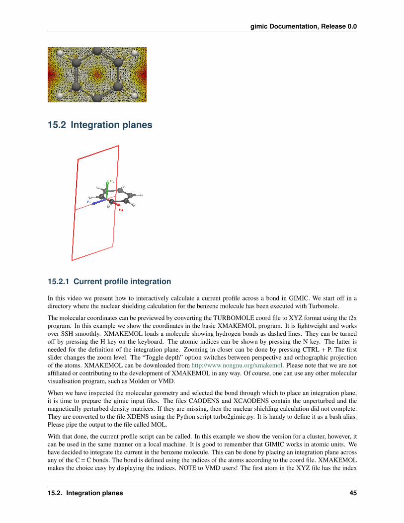
15.2 Integration planes

15.2.1 Current profile integration

In this video we present how to interactively calculate a current profile across a bond in GIMIC. We start off in adirectory where the nuclear shielding calculation for the benzene molecule has been executed with Turbomole.

The molecular coordinates can be previewed by converting the TURBOMOLE coord file to XYZ format using the t2xprogram. In this example we show the coordinates in the basic XMAKEMOL program. It is lightweight and worksover SSH smoothly. XMAKEMOL loads a molecule showing hydrogen bonds as dashed lines. They can be turnedoff by pressing the H key on the keyboard. The atomic indices can be shown by pressing the N key. The latter isneeded for the definition of the integration plane. Zooming in closer can be done by pressing CTRL + P. The firstslider changes the zoom level. The “Toggle depth” option switches between perspective and orthographic projectionof the atoms. XMAKEMOL can be downloaded from http://www.nongnu.org/xmakemol. Please note that we are notaffiliated or contributing to the development of XMAKEMOL in any way. Of course, one can use any other molecularvisualisation program, such as Molden or VMD.

When we have inspected the molecular geometry and selected the bond through which to place an integration plane,it is time to prepare the gimic input files. The files CAODENS and XCAODENS contain the unperturbed and themagnetically perturbed density matrices. If they are missing, then the nuclear shielding calculation did not complete.They are converted to the file XDENS using the Python script turbo2gimic.py. It is handy to define it as a bash alias.Please pipe the output to the file called MOL.

With that done, the current profile script can be called. In this example we show the version for a cluster, however, itcan be used in the same manner on a local machine. It is good to remember that GIMIC works in atomic units. Wehave decided to integrate the current in the benzene molecule. This can be done by placing an integration plane acrossany of the C = C bonds. The bond is defined using the indices of the atoms according to the coord file. XMAKEMOLmakes the choice easy by displaying the indices. NOTE to VMD users! The first atom in the XYZ file has the index

15.2. Integration planes 45

http://www.nongnu.org/xmakemol


one. VMD lists the indices starting from 0, so the given index needs to be increase by one. In this example we choseto integrate across the bond between atoms 4 and 5. According to our convention the atoms are entered in clockwiseorder, i.e. 4 – 5 instead of 5 – 4 in this case. The scripts asks for a possible suffix for the directory name. This canbe generally omitted, however sometimes it might be necessary to run calculations across the same bond but alongdifferent integration planes. In practice this means that if the suffix “modified” is entered, then the created calculationdirectory is current_profile_4.5_modified.

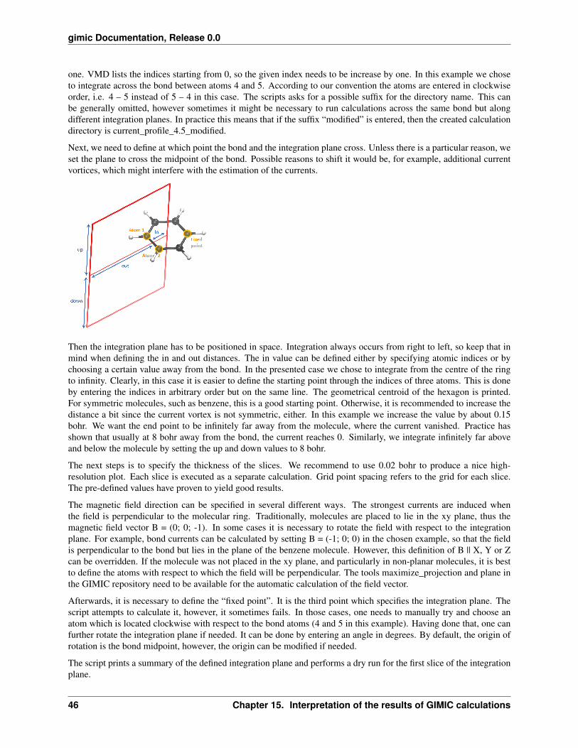
Next, we need to define at which point the bond and the integration plane cross. Unless there is a particular reason, weset the plane to cross the midpoint of the bond. Possible reasons to shift it would be, for example, additional currentvortices, which might interfere with the estimation of the currents.

Then the integration plane has to be positioned in space. Integration always occurs from right to left, so keep that inmind when defining the in and out distances. The in value can be defined either by specifying atomic indices or bychoosing a certain value away from the bond. In the presented case we chose to integrate from the centre of the ringto infinity. Clearly, in this case it is easier to define the starting point through the indices of three atoms. This is doneby entering the indices in arbitrary order but on the same line. The geometrical centroid of the hexagon is printed.For symmetric molecules, such as benzene, this is a good starting point. Otherwise, it is recommended to increase thedistance a bit since the current vortex is not symmetric, either. In this example we increase the value by about 0.15bohr. We want the end point to be infinitely far away from the molecule, where the current vanished. Practice hasshown that usually at 8 bohr away from the bond, the current reaches 0. Similarly, we integrate infinitely far aboveand below the molecule by setting the up and down values to 8 bohr.

The next steps is to specify the thickness of the slices. We recommend to use 0.02 bohr to produce a nice high-resolution plot. Each slice is executed as a separate calculation. Grid point spacing refers to the grid for each slice.The pre-defined values have proven to yield good results.

The magnetic field direction can be specified in several different ways. The strongest currents are induced whenthe field is perpendicular to the molecular ring. Traditionally, molecules are placed to lie in the xy plane, thus themagnetic field vector B = (0; 0; -1). In some cases it is necessary to rotate the field with respect to the integrationplane. For example, bond currents can be calculated by setting B = (-1; 0; 0) in the chosen example, so that the fieldis perpendicular to the bond but lies in the plane of the benzene molecule. However, this definition of B || X, Y or Zcan be overridden. If the molecule was not placed in the xy plane, and particularly in non-planar molecules, it is bestto define the atoms with respect to which the field will be perpendicular. The tools maximize_projection and plane inthe GIMIC repository need to be available for the automatic calculation of the field vector.

Afterwards, it is necessary to define the “fixed point”. It is the third point which specifies the integration plane. Thescript attempts to calculate it, however, it sometimes fails. In those cases, one needs to manually try and choose anatom which is located clockwise with respect to the bond atoms (4 and 5 in this example). Having done that, one canfurther rotate the integration plane if needed. It can be done by entering an angle in degrees. By default, the origin ofrotation is the bond midpoint, however, the origin can be modified if needed.

The script prints a summary of the defined integration plane and performs a dry run for the first slice of the integrationplane.

46 Chapter 15. Interpretation of the results of GIMIC calculations


(to be continued, and the video has to be finished)

15.2. Integration planes 47

gimic documentation

Documents