Gibbs posterior inference on the minimum clinicallyimportant difference

Nicholas Syring and Ryan MartinDepartment of Statistics

North Carolina State University(nasyring, rgmarti3)@ncsu.edu

June 28, 2017

Abstract

It is known that a statistically significant treatment may not be clinically sig-nificant. A quantity that can be used to assess clinical significance is called theminimum clinically important difference (MCID), and inference on the MCID isan important and challenging problem. Modeling for the purpose of inference onthe MCID is non-trivial, and concerns about bias from a misspecified parametricmodel or inefficiency from a nonparametric model motivate an alternative approachto balance robustness and efficiency. In particular, a recently proposed representa-tion of the MCID as the minimizer of a suitable risk function makes it possible toconstruct a Gibbs posterior distribution for the MCID without specifying a model.We establish the posterior convergence rate and show, numerically, that an ap-propriately scaled version of this Gibbs posterior yields interval estimates for theMCID which are both valid and efficient even for relatively small sample sizes.

Keywords and phrases: Clinical significance; loss function; M-estimation; model-free inference; posterior convergence rate.

1 Introduction

In clinical trials, often the main objective is assessing the efficacy of a treatment. However,experts have observed that statistical significance alone does not necessarily imply efficacy(Jacobson and Truax 1991). For instance, a study with high power can detect statisticallysignificant differences, but these may not translate to practical differences noticeable bythe patients. As a result, a cutoff value different than a statistical critical value is desiredthat can separate patients with and without clinically significant responses. This cutoffis called the minimum clinically important difference, or MCID for short (Jaescheke et al.1989). Accurate inference on the MCID is crucial for clinicians and health policy-makersto make educated judgments about the effectiveness of certain treatments. Indeed, theU. S. Food and Drug Administration held a special workshop in 2012 on methodologicaldevelopments towards improved inference on the MCID.1

1https://federalregister.gov/a/2012-27147

1

arX

iv:1

501.

0184

0v4

[st

at.M

E]

26

Jun

2017

The basic setup is that, in addition to a scalar diagnostic measure for each patient,which would be used to assess the statistical significance of a treatment, one also hasaccess to a “patient-reported outcome,” a binary indicator of whether or not the patientfelt that the treatment was beneficial. Then, roughly, the MCID is defined as the cutoffvalue such that, if the diagnostic measure exceeds this cutoff, then the patient is likely toobserve a benefit from the treatment. A more precise description of the problem setupis given in Section 2. The challenge in making inference on the MCID is in modelingthe joint distribution for the diagnostic measure and patient-reported outcome. Givena model, standard likelihood-based methods—Bayesian or non-Bayesian—could be used,but specifying a sound model is difficult because the MCID is a rather complicatedfunctional thereof. To avoid the potential bias caused by a misspecified parametric modeland the inefficiencies that result from an overly-complex nonparametric model, a model-free approach is an attractive alternative. Recently, Hedayat et al. (2015) propose aM-estimation framework for estimating the MCID, that does not require a model, butthe distribution theory needed to provide valid tests or confidence intervals for the MCIDbased on their approach is apparently out of reach.

In this paper, we show that a Gibbs posterior can provide inference on the MCID with-out requiring a likelihood, thus avoiding the modeling step and the risk of misspecificationwhile providing easy access to credible intervals, and that our new method compares fa-vorably to the existing M-estimation method in terms of both large-sample theory andfinite-sample performance. Construction of the Gibbs posterior takes advantage, first, ofthe representation in Hedayat et al. (2015) of the MCID as the minimizer of an expectedloss and, second, of the recent efforts in Bissiri et al. (2016) to describe a Bayesian-likeanalysis with a loss function in place of a likelihood. Our Gibbs posterior distributionis easy to compute and, with a suitable scaling, is shown to provide valid and efficientcredible intervals for the MCID.

Our focus in this paper is the MCID application, but some general comments aboutGibbs posteriors are worth mentioning. First, our problem is related to that of modelmisspecification, and it is known (e.g., Bunke and Milhaud 1998; De Blasi and Walker2013; Kleijn and van der Vaart 2006; Lee and MacEachern 2011; Ramamoorthi et al.2015; Walker 2013) that, asymptotically, the posterior distribution behaves reasonablyunder misspecification provided that it is Gibbs-like in the sense that the negative log-likelihood used resembles a suitable loss function; a nice example of this type is Sriramet al. (2013). Second, although misspecification is usually viewed as a bad thing, theremight be reasons to “misspecify on purpose.” For example, one may not wish to spendthe resources needed to flesh out a full model, including priors, and to compute the fullposterior when, ultimately, it will be marginalized to the parameter of interest. The Gibbsposterior described here has the advantage of being defined directly on the parameter ofinterest, simplifying both prior specifications and posterior computations.

The remainder of the paper is organized as follows. In Section 2 we introduce ournotation for the MCID problem and formulate its definition as a minimizer of an expectedloss. This leads naturally to the M-estimator proposed in Hedayat et al. (2015) and weimprove on their asymptotic convergence rate result in two ways: first, we improve therate and, second, we clarify the sense in which the rate depends on the local propertiesof the function defined in (3). In Section 3, after a motivating illustration, we defineour Gibbs posterior distribution for the MCID, and we go on to show that it, and the

2

corresponding posterior mean, converge at the same rate as the M-estimator of Hedayatet al. (2015). Simulation results are presented in Section 4, and the take away message isthat our Gibbs posterior, or a suitably scaled version thereof, provides quality inference onMCID, in terms of estimation accuracy and interval coverage and length. Some concludingremarks are given in Section 5, and technical details are given in the Appendix.

2 Minimum clinically important difference

2.1 Notation and definitions

In clinical trials for drugs or medical devices, it is standard to judge the effectiveness ofthe treatment based on statistical significance. However, it is possible that the treatmenteffect may be significantly different from zero in a statistical context, but the effect size isso small that the patients do not experience an improvement. To avoid the costs associ-ated with bringing to market a treatment that is not clinically effective, it is advantageousto bring the patients’ assessment of the treatment effect into the analysis. While the needfor a measure of clinical significance is well-documented (e.g., Kaul and Diamond 2010),it seems there is no universal definition of MCID and, consequently, there is no standardmethodology to make inference on it. Recent efforts in this direction were made by Shiuand Gatsonis (2008) and Turner et al. (2010). Hedayat et al. (2015) provide a mathe-matically convenient formulation, described next, in which the MCID is expressed as aminimizer of a suitable loss function.

Let Y ∈ {−1, 1} denote the patient reported outcome with “Y = 1” meaning thatthe treatment was effective and “Y = −1” meaning that the treatment was not effective.Let X be a continuous diagnostic measure taken on each patient. Let P denote the jointdistribution of (X, Y ), and p the marginal density of X with respect to Lebesgue measure.Given θ ∈ R, define the function `θ by

`θ(x, y) = 12{1− y sign(x− θ)}, (x, y) ∈ R× {−1, 1}, (1)

where sign(0) = 1, and write R(θ) = P`θ for the risk function, the expectation of `θ withrespect to the joint distribution P . Then the MCID, denoted by θ?, is defined as

θ? = arg minθR(θ). (2)

That is, the MCID is the minimizer of the risk function R, and depends on the distributionP in a rather complicated way. The intuition behind this definition is the alternativeexpression for R(θ):

R(θ) = P{Y 6= sign(X − θ)},i.e., θ? minimizes, over θ, the probability that sign(X − θ) disagrees with Y . In otherwords, sign(X − θ?) is the best predictor of Y in terms of minimum misclassificationprobability. Another representation of the MCID, as demonstrated by Hedayat et al.(2015), that will be convenient below is as a solution to the equation η(θ) = 1

2, where

η(x) = P (Y = 1 | X = x) (3)

is the conditional probability function. If η is continuous and strictly increasing, then θ?

will be the unique solution to the equation η(θ) = 12. If η is only upper semi-continuous,

3

then we may define θ? as inf{x : η(x) ≥ 12}, and an argument similar to that in Lemma 1

of Hedayat et al. (2015) shows that this θ? solves the optimization problem (2).

2.2 M-estimator and its large-sample properties

Hedayat et al. (2015) propose to estimate the MCID by minimizing an empirical risk.Let Pn = n−1

∑ni=1 δ(Xi,Yi) be the empirical measure, based on the observations {(Xi, Yi) :

i = 1, . . . , n}, where δ(x,y) is the point-mass measure at (x, y). Then the empirical risk isRn(θ) = Pn`θ, and an M-estimator of MCID is obtained by minimizing Rn(θ), i.e.,

θn = arg minθRn(θ). (4)

Computation of the estimator is straightforward since it takes only finitely many valuesdepending on the order statistics for the X-sample. Therefore, a simple grid search isguaranteed to quickly identify the minimizer θn.

A shortcoming of this approach is that, due to the discontinuity of the loss function, anasymptotic normality result for the M-estimator does not seem possible; see Section 2.3.Therefore, valid confidence intervals for the MCID based on the M-estimator are notcurrently available. This provides motivation for a Bayesian approach, where credibleintervals, etc, can be easily obtained, but some non-standard ideas are needed to dealwith the fact that θ is defined by a loss function, not a likelihood; see Section 3. Bootstrapmethods are available (see Section 4) but there is a general concern about their validitybecause the rate is not the usual n−1/2.

Consistency and convergence rates for the M-estimator θn have been studied by He-dayat et al. (2015). The rates rely on the local behavior of the function η and of themarginal distribution of X around θ?. In Theorem 1, we clarify and substantially im-prove upon the rate result given in Hedayat et al. (2015). Our assumptions here are moreefficient than theirs, and we discuss these differences below.

Assumption 1. The marginal density p of X is continuous and bounded away from 0 and∞ on an interval containing θ?.

Assumption 2. The function η in (3) is non-decreasing, upper semi-continuous, and sat-isfies η(θ) > η(θ?) for all θ > θ?. Furthermore, there exists constants c > 0, and γ ≥ 0such that

min |η(θ? ± ε)− η(θ?)| > cεγ, for all small ε > 0, (5)

where “min” is with respect to the two choices in “±.”

We interpret γ as an“ease of identification” index, where smaller γ means that the ηfunction is, in a certain sense, changing more rapidly near θ?, making the MCID easierto identify. In particular, if η has a jump discontinuity at θ?, then γ = 0, and thiscorresponds to the easiest case; if η is differentiable at θ?, then γ = 1, the most difficultcase; and if η is continuous but not differentiable at θ?, then γ ∈ (0, 1), an intermediatecase. For a quick example of the latter case, intermediate ease of identification, fixα, β ∈ (0, 1), α ≥ β, and define η(x), x ∈ [−1, 1] as

η(x) =

{12(1− |x|α), if x ∈ [−1, 0),

12(1 + xβ), if x ∈ [0, 1].

.

4

Clearly, the MCID is θ? = 0, η is continuous but not differentiable there, and (5) holdswith γ = α. Although this “ease of identification” index is non-standard, it appearsto be the key determinant of the convergence rate. Indeed, the convergence rate of theM-estimator in Theorem 1 below improves as γ decreases to 0, explaining why we callγ = 0 and γ = 1 the “easiest” and the “most difficult” cases, respectively.

Theorem 1. Under Assumptions 1–2, the M-estimator θn in (4) satisfies θn − θ? =OP (n−r) as n→∞, where r = (1 + 2γ)−1, and γ is defined in (5).

Proof. See Appendix A.2.

Our assumptions are different than those in the M-estimator convergence rate theoremof Hedayat et al. (2015), so some comments are in order. In particular, they impose aHolder continuity condition on η, as well as a “low noise assumption,” in Equation (4)in their paper, which upper-bounds the P -probability assigned to events of the form{|η(X) − 1

2| ≤ ξ}. This implicitly requires that η not be too flat near θ?, just like our

condition (5), and together with their Holder condition, they derive a locally uniformlower bound on the risk difference R(θ)−R(θ?), similar to the one we derive in Lemma 2in the Appendix. However, our approach and more-direct assumptions appear to be moreefficient, because we get a better lower bound on R(θ)−R(θ?) and, consequently, a betterconvergence rate. Indeed, in the case where η is differentiable at θ?, we obtain a raten−1/3 whereas Hedayat et al. (2015) obtains n−1/5 (up to logarithmic terms). Similarly,for that example above with powers α ≥ β, we obtain a rate n−r, with r = (1 + 2α)−1

whereas Hedayat et al. (2015) obtains n−r′, with r′ = {2(1 + 2α)− β/α}−1. So, besides

showing how the rate depends critically on the “ease of identification” index γ, theseexamples also highlight the significant improvements in our rates.

2.3 On smoothed versions of the problem

It was mentioned above that Rn(θ) not being smooth causes some problems in termsof limit distribution theory, etc. It would, therefore, be tempting to replace that non-smooth loss function by something smooth, and hope that the approximation error isnegligible. One idea would be to introduce a nice parametric model for this problem. Forexample, consider a binary regression model, where η(x) = F (β0 + β1x) and F is somespecified distribution function, such as logistic or normal. Then the MCID correspondsto the median lethal dose (e.g., Agresti 2002; Kelly 2001). Such a model is smooth soasymptotic normality holds. However, unless the true P has the specified form, there willbe non-zero bias that cannot be overcome, even asymptotically; see Section 3.1. Sincethe bias is unknown, sampling distribution concentration around the wrong point cannotbe corrected, so is of little practical value.

A slightly less extreme smoothing of the problem is to make a minor adjustment to theoriginal loss function `θ. As in Hedayat et al. (2015), introduce a smoothing parameterτ > 0 and consider

`τθ(x, y) = min{

1,[1− τ−1 y sign(x− θ)

]+},

where u+ = max(u, 0) denotes the positive part. Write Rτ (θ) = P`τθ . Based on argumentsin Hedayat et al. (2015), it can be shown that Rτ (θ) converges uniformly to R(θ) as

5

τ → 0, so, for small τ , the minimizer of Rτ would be close to θ?. For fixed τ , one candefine Rτ

n(θ) = Pn`τθ just as before and consider an M-estimator θτn = arg minθ Rτn(θ).

An asymptotic normality result for θτn is available, but the proper centering is not at θ?

and the asymptotic variance is inversely proportional to τ . So, one could take τ = τnvanishing with n in an effort to remove the bias, but a price must be paid in terms of thevariance. Again, having an asymptotic normality result with either an unknown non-zerobias or a very large variance is of little practical value.

Based on these remarks, apparently there is no hope in trying to smooth out theproblem to make it a standard one with the usual asymptotic distribution theory. So, inorder to construct useful interval estimates, etc, one needs some different ideas.

3 A Gibbs posterior for MCID

3.1 Motivation

As discussed above, estimation of the MCID can be achieved without specifying a model,but the distribution theory needed to develop valid interval estimates is lacking. ABayesian approach automatically provides uncertainty quantification, but it requires amodel for the joint distribution P . To motivate our model-free Gibbs posterior develop-ment that follows, we demonstrate the apparent sensitivity of some “standard” Bayesianposterior distributions—parametric and nonparametric—to the underlying P . To beclear, we do not claim that Bayesian methods, in general, are inappropriate for thisMCID problem, only that the posterior can be particularly sensitive to the choice ofmodel for P so a less-sensitive approach, if one were available, would be attractive.

Suppose we begin our analysis with a model for P given by a joint density/massfunction fβ(x, y), depending on some parameter β, possibly infinite-dimensional, whichwould typically be different from θ. Given a prior for β, a posterior distribution for βcan be readily obtained via Bayes theorem, which can be marginalized to get a posteriordistribution for θ. In particular, logistic regression is a sort of black-box approach to studythe relationship between a binary response and a quantitative predictor, so consider aBernoulli model for Y , given X = x, where the success probability is F (β0 + β1x), whereF is the standard logistic distribution function. In this case, the MCID is just the medianlethal dose, i.e., θ = −β0/β1. The choice of the logit link function F is quite rigid, but amore flexible nonparametric approach is available (Choudhuri et al. 2007).

There are pros and cons to both of the approaches just described. Assuming that thelogistic regression model is well-specified, inference on the MCID ought to be efficient.However, if the model is misspecified in some way, then there could be non-negligible biasthat cannot be overcome, even asymptotically. The model that treats the link functionnonparametrically is more flexible and, therefore, less prone to bias, but at the cost ofan increased computational burden and lower efficiency, i.e., posterior for the MCID ismore diffuse. Old-fashioned modeling would be a middle-ground between the extremes ofa black-box logistic regression and an overly complex nonparametric regression, but thiscertainly requires some investment and, unfortunately, is not foolproof. Our proposedGibbs approach is an alternative middle-ground, one that avoids misspecification bias,computational and statistical inefficiency, and modeling investment.

6

For clarity, we give an illustration of the points just raised. In particular, we compareour Gibbs posterior defined in Section 3.2 to both a standard Bayesian logistic regressionand a nonparametric binary regression (Choudhuri et al. 2007). For the Bayesian logisticregression we consider the vague priors for (β0, β1) given in Polson et al. (2013), but ourresults do not appear to be sensitive to this choice. Let us suppose that the true modelgenerating data (X, Y ) has a distribution function F for X and, given X = x, Y isBernoulli ±1 with success probability F (x). We will consider two different forms of F ,both two-component normal mixtures:

X ∼ 0.7N(−1, 1) + 0.3N(1, 1) and X ∼ 0.7N(−1, 1) + 0.3N(3, 1).

The true MCID may be calculated by solving (3); it is equal to the median of the Xdistribution, specifically θ? = −0.514 in the first example and θ? = −0.434 in the secondexample. Of course, the logistic regression model is misspecified, but the nonparametricmodel should not be affected by this. But how will they perform in the two examples?

Plots of the marginal posterior density for θ are shown in Figure 1 for a simulated dataset of size n = 500 obtained from each of the three methods—Gibbs, logistic regression,and nonparametric—one for each marginal distribution forX. In Panel (a) we see that theposterior distributions for all three models put their mass near the true MCID. However,in Panel (b) we see that the posterior distribution for the Bayesian logistic regression isclearly biased away from the true MCID. The nonparametric Bayesian posterior is veryspread out, making it less informative for inference on the MCID. Our Gibbs approach,however, is right on the mark in both cases, suggesting that it is neither sensitive to modelmisspecification nor does it suffer from the inefficiency of the nonparametric approach.

3.2 Posterior construction

In contrast with a likelihood-based approach, a Gibbs model does not require specificationof the probability model P . A Gibbs model consists of a risk function connecting dataand parameter, here (1), and a prior for the parameter. Bissiri et al. (2016) consider aGibbs model that boils down to treating the scaled empirical risk function nRn(θ) like anegative log-likelihood and constructing the posterior distribution as usual. That is, ourGibbs posterior distribution for θ is given by

Πn(A) =

∫Ae−nRn(θ) Π(dθ)∫

R e−nRn(θ) Π(dθ)

, A ⊂ R, (6)

where Rn(θ) = Pn`θ is the empirical risk defined above, and Π is the prior distributionfor θ. Note that the use of the actual loss function defining the MCID means that wehave not introduced any bias. Moreover, we are only required to do prior specificationand posterior computations directly on the θ-space, i.e., there are no additional nuisanceparameters that need priors but will ultimately be marginalized away.

Since the empirical risk function Rn(θ) is bounded away from zero and infinity, thetails of the posterior match those of the prior. However, data cannot support a value ofθ outside the range of the X observations so, in practice, we will implicitly restrict theposterior to that range. This adjustment is not necessary for our theoretical analysis.

7

−1.0 −0.8 −0.6 −0.4 −0.2 0.0

02

46

8

MCID

Den

sity

GibbsNonpar.Logistic

(a) X ∼ 0.7N(−1, 1) + 0.3N(1, 1)

−1.0 −0.5 0.0 0.5 1.0

02

46

8

MCID

Den

sity

GibbsNonpar.Logistic

(b) X ∼ 0.7N(−1, 1) + 0.3N(3, 1)

Figure 1: Plots of (kernel estimates of) the posterior density for MCID. “Nonpar.” cor-responds to the nonparametric binary regression model; “Logistic” corresponds to theposterior based on the genuine Bayes logistic model; “Gibbs” is the proposed likelihood-free Bayesian posterior; true MCID θ? marked with a dotted vertical line.

3.3 Posterior convergence rates

The Gibbs posterior convergence rate describes, roughly, the size of the neighborhoodaround θ? that it assigns nearly all its mass as n → ∞. An important consequenceof a posterior convergence rate result is that typical posterior summaries also have niceconvergence rate properties; see Corollary 1.

It turns out that the posterior convergence rate result holds under virtually the sameconditions as Theorem 1 for the M-estimator. The only additional condition neededconcerns the prior, and it is very mild.

Assumption 3. The prior distribution Π for θ has a density π which is continuous andbounded away from zero in a neighborhood of θ?.

Theorem 2. Under Assumptions 1–3, the Gibbs posterior distribution Πn in (6) satisfiesΠn(An) = oP (1) as n → ∞, where An = {θ : |θ − θ?| > ann

−r}, r = (1 + 2γ)−1 for γ in(5), and an is any diverging sequence.

Proof. See Appendix A.3.

Corollary 1. Under the conditions of Theorem 2, if the prior mean for θ exists, thenthe posterior mean θn satisfies θn − θ? = OP (n−r) as n→∞.

Proof. See Appendix A.3.

8

3.4 On scaling the loss function

A subtle point is that the loss function `θ has an arbitrary scale. That is, the problemof inference on the risk minimizer is unchanged if we replace `θ with ω`θ for any ω > 0.While this has no effect on the M-estimator, it does have an effect on our Gibbs posterior.Based on our experience, the posterior distribution actually tends to be quite narrow,so the posterior concentration rates seem to be driven primarily by the “center” of theposterior and, to a lesser extent, by the “spread.” As Bissiri et al. (2016) explain, it isimportant to scale the loss in some way. In Lemma 1 below, we show that the Gibbsposterior may be scaled by a vanishing sequence without sacrificing the convergence ratein Theorem 2. Our numerical results in Section 4 show that taking the scale to bevanishing accomplishes the goal of calibrating the credible intervals without affecting theaccuracy of the posterior mean estimator.

Lemma 1. Under Assumptions 1–3, with r = (1 + 2γ)−1 and γ defined in (5), theconclusion of Theorem 2 holds if the loss function `θ is scaled by a sequence ωn thatvanishes strictly more slowly than n−γr.

Proof. Similar to the proof of Theorem 2 in Appendix A.3.

In our experience, with continuous η, we found that a scale value of approximatelyωn = cn−1/4, for c ∈ (1, 2), worked well in terms of credible interval calibration. To avoidmaking an ad hoc choice of constant, we employ the algorithm in Syring and Martin(2016a). Our scaling algorithm is applied to each simulated data set, producing a dif-ferent, data-dependent value of the scale parameter each time. Briefly, ωn is determinedby solving the equation that sets the Gibbs posterior credible interval coverage proba-bility equal to the desired confidence level. The algorithm utilizes standard techniquesincluding stochastic approximation, MCMC, and bootstrapping. In our simulations, thealgorithm succeeds in producing approximately calibrated credible intervals. In the nu-merical examples that follow, the ωn selected by the algorithm is, on average, roughly1.5n−1/4, which is consistent with the result in Lemma 1.

4 Numerical examples

We consider four examples to illustrate the performance of our Gibbs posterior for theMCID. Each example has a different marginal distribution for X:

Example 1. X ∼ 0.7N(−1, 1) + 0.3N(1, 1);

Example 2. X ∼ N(1, 1);

Example 3. X ∼ Unif(−2, 4).

Example 4. X ∼ Gamma(2, 0.5).

These examples cover a variety of distributions: bimodal, normal, flat, and skewed. Ineach example, we take n independent samples from the respective marginal distributions,and then, given Xi = xi, take Yi as a ±1 Bernoulli with probability F (xi), i = 1, . . . , n,where F is the distribution function of X and Ber(p) denotes a Bernoulli distributionwith success probability p. In our case, the relevant summaries are the bias and standard

9

deviation of the estimators, and the coverage probability and length of the 90% intervalestimates. We considered three sample sizes, namely, n = 250, 500, 1000, and the resultsin Tables 1–2 are based on 1000 Monte Carlo samples. We compare the performanceof our Gibbs posterior, using the scaling algorithm in Syring and Martin (2016a) and aflat prior for θ, to a baseline method, namely, the M-estimator and the correspondingpercentile bootstrap confidence intervals.

Table 1 shows the empirical bias and standard deviation for both the M-estimatorand the Gibbs posterior mean while Table 2 shows the empirical coverage probabilityand length for the 90% interval estimates based on bootstrapping the M-estimator andon the Gibbs posterior sample. Here we see that the additional flexibility of being able tochoose the scaling parameter/sequence provides approximately calibrated posterior cred-ible intervals for each n. Overall, the performance of our Gibbs posterior is comparable tothe M-estimator+bootstrap, the take-away message being that a Bayesian-like approachneed not sacrifice desirable frequentist properties. Two comments are in order. First,if reliable prior information is available, which is possible in medical applications wherestudies are replicated, then this can be readily incorporated into our analysis, naturallyproviding some improvements. For example, if an accurate, informative N(−0.5, 1) prior isused in Example 1 for n = 250, the bias is reduced to 0.01 and the credible interval lengthis reduced to 0.83 with 0.90 coverage, an improvement over bootstrap confidence inter-vals. Second, the desirable frequentist properties are not automatic for other Bayesianapproaches; for instance, the Bayesian logistic regression model described in Section 3.1has mean square error equal to 0.07 and 0.20 in Examples 3 and 4, respectively, withn = 250, compared to 0.015 and 0.011 for the Gibbs posterior mean.

5 Conclusion

In this paper, motivated by a real application in medical statistics, we have explored theuse of a Gibbs posterior distribution for inference. In certain applications, like this MCIDproblem, the statistician may be reluctant to use a likelihood-based model due to fearof misspecification, computational difficulty, or for some other reason. The Gibbs modeloffers an alternative Bayesian-like approach that does not require a probability model,thus avoiding some of these potential challenges, and we think that this advantage maymake Gibbs models widely applicable. As we have demonstrated, the proposed Gibbsposterior is theoretically justified and provides quality point and interval estimates inpractice. So, in a certain sense, our Gibbs posterior provides the best of both worlds:that is, we get a theoretically justifiable posterior distribution without the unnecessarymodeling and computations and without worry of model misspecification.

The technical details in this paper are kept relatively simple due to the fact that θ isa scalar and `θ is bounded, but our methods can be applied more generally. For example,Hedayat et al. (2015) proposed a generalization of the MCID problem in which θ isactually a function of some other covariates, thereby making the MCID “personalized”in a certain sense. We are working on extending both the theory and the computationalmethods presented here to this more general case. A recent paper (Syring and Martin2016b) develops a nonparametric Gibbs posterior for inference on a function and prove asmoothness-adaptive convergence rate theorem. The techniques developed therein may

10

Example Method n = 250 n = 500 n = 10001 M-estimator 0.03 (0.21) 0.01 (0.16) 0.01 (0.12)

Gibbs 0.03 (0.22) 0.01 (0.17) 0.01 (0.13)

2 M-estimator 0.02 (0.16) 0.02 (0.12) 0.01 (0.10)Gibbs 0.00 (0.15) 0.01 (0.12) 0.00 (0.10)

3 M-estimator 0.01 (0.12) 0.01 (0.10) 0.01 (0.08)Gibbs 0.01 (0.12) 0.00 (0.10) 0.00 (0.07)

4 M-estimator 0.01 (0.12) 0.01 (0.09) 0.01 (0.07)Gibbs 0.03 (0.10) 0.02 (0.08) 0.01 (0.06)

Table 1: Absolute empirical bias (and standard deviation) for the M-estimator in Hedayatet al. (2015) and our proposed Gibbs posterior mean.

Example Method n = 250 n = 500 n = 10001 M+Boot 0.91 (0.86) 0.91 (0.69) 0.93 (0.53)

Gibbs 0.89 (0.89) 0.89 (0.69) 0.91 (0.55)

2 M+Boot 0.91 (0.60) 0.91 (0.48) 0.92 (0.38)Gibbs 0.89 (0.61) 0.91 (0.50) 0.90 (0.38)

3 M+Boot 0.90 (0.47) 0.90 (0.38) 0.91 (0.30)Gibbs 0.91 (0.48) 0.90 (0.37) 0.90 (0.30)

4 M+Boot 0.92 (0.39) 0.92 (0.31) 0.92 (0.25)Gibbs 0.91 (0.41) 0.90 (0.31) 0.90 (0.24)

Table 2: Empirical coverage probability (and mean length) of 90% confidence intervalbased on bootstrapping the M-estimator in Hedayat et al. (2015) and the 90% credibleinterval from our proposed Gibbs posterior.

be able to be applied in the personalized MCID problem.

Acknowledgments

The authors are grateful to the Editor, Associate Editor, and referees for their helpfulcomments on a previous version of this manuscript. This work is partially supported bythe U. S. Army Research Offices, Award #W911NF-15-1-0154.

11

A Technical details and proofs

A.1 Preliminary results

Here, for the sake of completeness, we summarize some basic facts about the empiricalrisk function Rn(θ) = Pn`θ and the risk R(θ) = P`θ. Details will be given only for thoseresults not taken directly from Hedayat et al. (2015).

First, we consider properties of the expected loss difference, R(θ)−R(θ?). By definitionof θ?, and Assumption 2 about η, we know the difference is strictly positive except atθ = θ?. To see this, Hedayat et al. (2015) show that

R(θ)−R(θ?) = 2

∫ θ

θ?{η(x)− 1

2}p(x) dx. (7)

Moreover, by continuity of p in Assumption 1 and almost everywhere continuity of ηderived from Assumption 2, we can see that the derivative of R(θ) − R(θ?) could bezero only at θ = θ?, which implies that the function is uniformly bounded away fromzero outside an interval containing θ?. This latter point is important because asymptoticresults of, say, the M-estimator require that the minimizer θ? be “well-separated” (e.g.,van der Vaart 1998, Theorem 5.7). We seek a lower bound on the expected loss differencein (7) for parameter values far from the MCID. That is, we want to calculate

inf|θ−θ?|>δ

R(θ)−R(θ?). (8)

The following result is new and allows us to improve upon the rate given for the M-estimator in Hedayat et al. (2015).

Lemma 2. Under Assumptions 1–2, there exists a constant c > 0 such that (8) is lower-bounded by cδ1+γ for all sufficiently small δ > 0.

Proof. Since η(x) is non-decreasing in x (Assumption 2) the infimum in (8) occurs at theboundary, either at θ? + δ or at θ? − δ. The two cases can be handled similarly, so wegive the argument only for the case that the infimum is attained at θ? + δ. Monotonicityof η implies that η(θ? + δ) > η(θ? + δ/2) > η(θ?). Also, according to Assumption 1, themarginal density p is bounded away from zero on an interval containing θ?, so let b be theinfimum over the interval [θ?− δ, θ?+ δ]. Using the expression in (7), we can lower-boundR(θ? + δ)−R(θ?) as follows:

R(θ? + δ)−R(θ?) =

∫ θ?+δ

θ?{2η(x)− 1}p(x) dx

=(∫ θ?+δ/2

θ?+

∫ θ?+δ

θ?+δ/2

){2η(x)− 1}p(x) dx

> b δ {η(θ? + δ/2)− 12}

≥ b δ {η(θ? + δ/2)− η(θ?)}.

By Assumption 2, in particular, condition (5), we have that the difference in the lastdisplay is bounded below by c1(δ/2)γ. Plugging this in at the end of the above displaygives the advertised lower bound, cδ1+γ, where c = bc1/2

γ.

12

Second, we need some approximation properties of the class of functions

Lδ := {`θ − `θ? : |θ − θ?| < δ}, δ > 0.

Hedayat et al. (2015) shows, using the standard partition in the classical Glivenko–Cantelli theorem (e.g., van der Vaart 1998, Example 19.6), that the L1(P ) ε-bracketingnumber N[ ](ε,L∞, L1(P )) is proportional to ε−1. This is enough to show that the classL∞ is Glivenko–Cantelli, from which a uniform law of large numbers follows. However,better rates can be obtained by using a local bracketing, i.e., of Lδ for finite δ, andAssumptions 1–2. Such considerations allow us to remove the unnecessary logarithmicterm on the rate presented in Theorem 1 of Hedayat et al. (2015).

Lemma 3. N[ ](ε,Lδ, L1(P )) . δ/ε.

Proof. For the standard Glivenko–Cantelli theorem partition, which is used in Hedayatet al. (2015), one needs to partition the interval [0, 1] into k intervals of length less thanε, so k must be greater than 1/ε, but can be taken less than 2/ε. By Assumption 1, wehave that δ . P (|X − θ?| < δ) . δ. For the local bracketing, this means we only needto partition an interval of length proportional to δ into intervals of length less than ε.Therefore, the total number of intervals is . δ/ε, as was to be shown.

From this and the fact that the brackets are pairs of indicator functions, we can get abound on the L2(P ) bracket number, i.e., N[ ](ε,Lδ, L2(P )) . (δ/ε)2; see Example 19.6in van der Vaart (1998). Then the bracketing integral is

J[ ](δ,Lδ, L2(P )) :=

∫ δ

0

{logN[ ](ε,Lδ, L2(P ))}1/2 dε . δ. (9)

Finally, we will need a maximal inequality for the empirical process Gn(`θ− θθ?) for θnear θ?. Hedayat et al. (2015) show that g(θ) = I{|θ−θ?|≤δ} is an envelop function for Lδ,with ‖g‖L2(P ) . δ1/2. Then, given the bound (9) on the bracketing integral, the maximalinequality in Corollary 19.35 of van der Vaart (1998) gives the following.

Lemma 4. P{sup|θ−θ?|<δ |Gn(`θ − `θ?)|} . δ1/2.

A.2 Proofs from Section 2.2

Proof of Theorem 1. Similar to the proof of Theorem 2 in Wong and Shen (1995) and ofTheorem 5.52 in van der Vaart (1998). The M-estimator θn, the global minimizer of Rn,satisfies Rn(θn) ≤ Rn(θ?) + ζn for any ζn. Let K > 0 be as in Lemma 6 in Appendix A.3,and take ζn = Ks1+γn , where sn = ann

−r, r = (1+2γ)−1, and an is any divergent sequence.Then we have that

|θn − θ?| > sn =⇒ sup|θ−θ?|>sn

{Rn(θ?)−Rn(θ)} ≥ −Ks1+γn .

By Lemma 6, the latter event has vanishing P -probability, which implies that P (|θ−θ?| >sn)→ 0. Therefore, θn − θ? = oP (sn) or, since an is arbitrary, θn − θ? = OP (n−r).

13

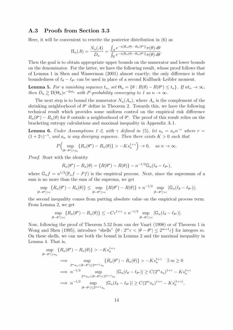
A.3 Proofs from Section 3.3

Here, it will be convenient to rewrite the posterior distribution in (6) as

Πn(A) =Nn(A)

Dn

=

∫Ae−n[Rn(θ)−Rn(θ

?)]π(θ) dθ∫R e−n[Rn(θ)−Rn(θ?)]π(θ) dθ

.

Then the goal is to obtain appropriate upper bounds on the numerator and lower boundson the denominator. For the latter, we have the following result, whose proof follows thatof Lemma 1 in Shen and Wasserman (2001) almost exactly; the only difference is thatboundedness of `θ − `θ? can be used in place of a second Kullback–Leibler moment.

Lemma 5. For a vanishing sequence tn, set Θn = {θ : R(θ)−R(θ?) ≤ tn}. If ntn →∞,then Dn & Π(Θn)e−2ntn with P -probability converging to 1 as n→∞.

The next step is to bound the numerator Nn(An), where An is the complement of theshrinking neighborhood of θ? define in Theorem 2. Towards this, we have the followingtechnical result which provides some uniform control on the empirical risk differenceRn(θ?)−Rn(θ) for θ outside a neighborhood of θ?. The proof of this result relies on thebracketing entropy calculations and maximal inequality in Appendix A.1.

Lemma 6. Under Assumptions 1–2, with γ defined in (5), let sn = ann−r where r =

(1 + 2γ)−1, and an is any diverging sequence. Then there exists K > 0 such that

P(

sup|θ−θ?|>sn

{Rn(θ?)−Rn(θ)} > −Ks1+γn

)→ 0, as n→∞.

Proof. Start with the identity

Rn(θ?)−Rn(θ) = {R(θ?)−R(θ)} − n−1/2Gn(`θ − `θ?),

where Gnf = n1/2(Pnf − Pf) is the empirical process. Next, since the supremum of asum is no more than the sum of the suprema, we get

sup|θ−θ?|>ε

{Rn(θ?)−Rn(θ)} ≤ sup|θ−θ?|>ε

{R(θ?)−R(θ)}+ n−1/2 sup|θ−θ?|>ε

|Gn(`θ − `θ?)|;

the second inequality comes from putting absolute value on the empirical process term.From Lemma 2, we get

sup|θ−θ?|>ε

{Rn(θ?)−Rn(θ)} ≤ −Cε1+γ + n−1/2 sup|θ−θ?|>ε

|Gn(`θ − `θ?)|.

Now, following the proof of Theorem 5.52 from van der Vaart (1998) or of Theorem 1 inWong and Shen (1995), introduce “shells” {θ : 2mε < |θ − θ?| ≤ 2m+1ε} for integers m.On these shells, we can use both the bound in Lemma 2 and the maximal inequality inLemma 4. That is,

sup|θ−θ?|>sn

{Rn(θ?)−Rn(θ)} > −Ks1+γn

=⇒ sup2msn<|θ−θ?|≤2m+1sn

{Rn(θ?)−Rn(θ)} > −Ks1+γn ∃ m ≥ 0

=⇒ n−1/2 sup2msn<|θ−θ?|<2m+1sn

|Gn(`θ − `θ?)| ≥ C(2msn)1+γ −Ks1+γn

=⇒ n−1/2 sup|θ−θ?|≤2m+1sn

|Gn(`θ − `θ?)| ≥ C(2msn)1+γ −Ks(1+γ)n ,

14

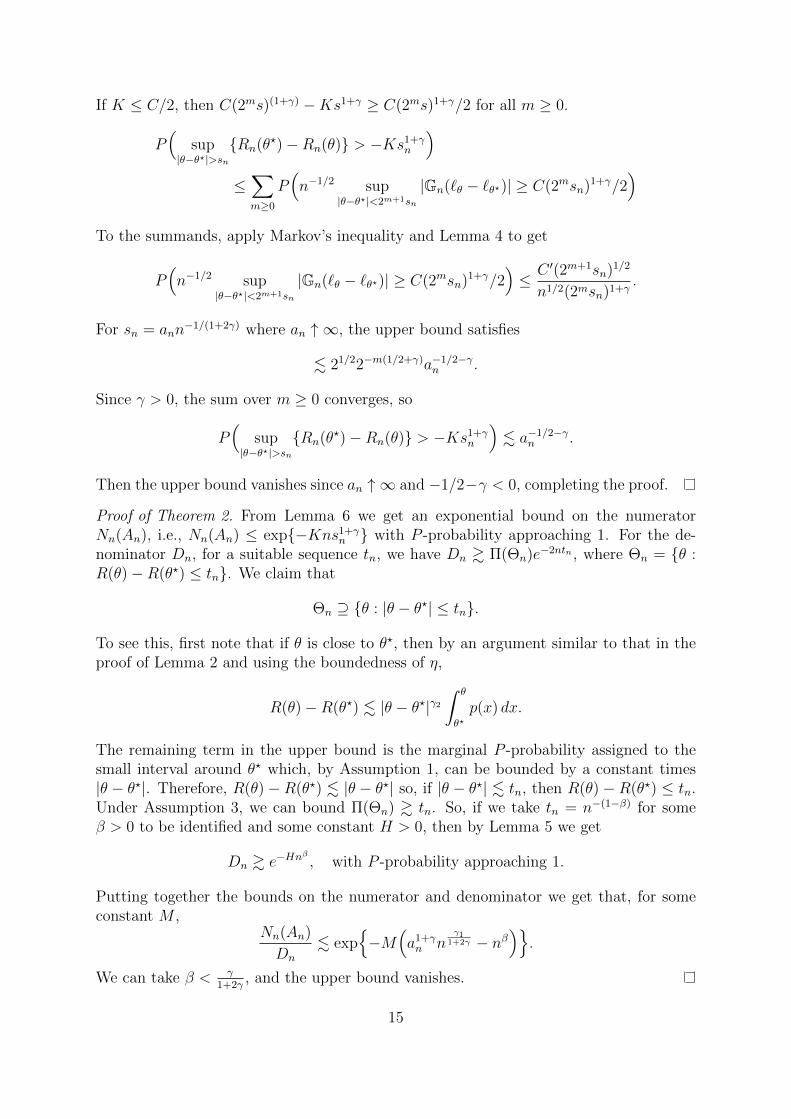
If K ≤ C/2, then C(2ms)(1+γ) −Ks1+γ ≥ C(2ms)1+γ/2 for all m ≥ 0.

P(

sup|θ−θ?|>sn

{Rn(θ?)−Rn(θ)} > −Ks1+γn

)≤∑m≥0

P(n−1/2 sup

|θ−θ?|<2m+1sn

|Gn(`θ − `θ?)| ≥ C(2msn)1+γ/2)

To the summands, apply Markov’s inequality and Lemma 4 to get

P(n−1/2 sup

|θ−θ?|<2m+1sn

|Gn(`θ − `θ?)| ≥ C(2msn)1+γ/2)≤ C ′(2m+1sn)1/2

n1/2(2msn)1+γ.

For sn = ann−1/(1+2γ) where an ↑ ∞, the upper bound satisfies

. 21/22−m(1/2+γ)a−1/2−γn .

Since γ > 0, the sum over m ≥ 0 converges, so

P(

sup|θ−θ?|>sn

{Rn(θ?)−Rn(θ)} > −Ks1+γn

). a−1/2−γn .

Then the upper bound vanishes since an ↑ ∞ and −1/2−γ < 0, completing the proof.

Proof of Theorem 2. From Lemma 6 we get an exponential bound on the numeratorNn(An), i.e., Nn(An) ≤ exp{−Kns1+γn } with P -probability approaching 1. For the de-nominator Dn, for a suitable sequence tn, we have Dn & Π(Θn)e−2ntn , where Θn = {θ :R(θ)−R(θ?) ≤ tn}. We claim that

Θn ⊇ {θ : |θ − θ?| ≤ tn}.

To see this, first note that if θ is close to θ?, then by an argument similar to that in theproof of Lemma 2 and using the boundedness of η,

R(θ)−R(θ?) . |θ − θ?|γ2∫ θ

θ?p(x) dx.

The remaining term in the upper bound is the marginal P -probability assigned to thesmall interval around θ? which, by Assumption 1, can be bounded by a constant times|θ − θ?|. Therefore, R(θ)− R(θ?) . |θ − θ?| so, if |θ − θ?| . tn, then R(θ)− R(θ?) ≤ tn.Under Assumption 3, we can bound Π(Θn) & tn. So, if we take tn = n−(1−β) for someβ > 0 to be identified and some constant H > 0, then by Lemma 5 we get

Dn & e−Hnβ

, with P -probability approaching 1.

Putting together the bounds on the numerator and denominator we get that, for someconstant M ,

Nn(An)

Dn

. exp{−M

(a1+γn n

γ11+2γ − nβ

)}.

We can take β < γ1+2γ

, and the upper bound vanishes.

15

Proof of Corollary 1. Set sn = ann−r for an an arbitrary divergent sequence. Next, define

sn = ann−r(γ), where an is such that an/an → 0, e.g., an = log an. Now partition R as

{θ : |θ − θ?| ≤ sn} ∪ {θ : |θ − θ?| > sn}, and write

|θn − θ?| ≤∫|θ − θ?|Πn(dθ) ≤ sn +

∫|θ−θ?|>sn

|θ − θ?|Πn(dθ), (10)

where the first inequality is by Jensen. From the proof of Theorem 2, the posterior awayfrom θ? is bounded by the prior times some Zn = oP (1), uniformly in θ. That is,∫

|θ−θ?|>sn|θ − θ?|Πn(dθ) ≤ Zn

∫|θ − θ?|Π(dθ).

In fact, we can bound Zn more precisely:

Zn . exp{−M

(a1+γn n

γ1+2γ − nβ

)}, sufficiently small β > 0.

Dividing through (10) by sn we get that s−1n |θn − θ?| is bounded by a constant times

an/an + e−ζn∫|θ − θ?|Π(dθ),

where ζn = Ma1+γn nγ

1+2γ −Mnβ + log an− r log n. The first term in the upper bound goesto zero by the choice of an. The second term goes to zero provided that the prior meanexists and ζn →∞ as n→∞. We assumed the former condition, and the latter can beeasily arranged by choosing β sufficiently small, so θn − θ? = oP (sn).

References

Agresti, A. (2002). Categorical Data Analysis. Wiley-Interscience [John Wiley & Sons],New York, second edition.

Bissiri, P., Holmes, C., and Walker, S. (2016). A general framework for updating beliefdistributions. J. R. Stat. Soc. Ser. B Stat. Methodol., 78(5):1103–1130.

Bunke, O. and Milhaud, X. (1998). Asymptotic behavior of Bayes estimates under pos-sibly incorrect models. Ann. Statist., 26(2):617–644.

Choudhuri, N., Ghosal, S., and Roy, A. (2007). Nonparametric binary regression using aGaussian process prior. Stat. Methodol., 4:227–243.

De Blasi, P. and Walker, S. G. (2013). Bayesian asymptotics with misspecified models.Statist. Sinica, 23:169–187.

Hedayat, S., Wang, J., and Xu, T. (2015). Minimum clinically important difference inmedical studies. Biometrics, 71:33–41.

Jacobson, N. and Truax, P. (1991). Clinical significance: a statistical approach to defininga meaningful change in psychotherapy research. J. Consult. Clin. Psych., 59:12–19.

16

Jaescheke, R., Signer, J., and Guyatt, G. (1989). Measurement of health status: ascer-taining the minimum clinically important difference. Control. Clin. Trials, 10:407–415.

Kaul, S. and Diamond, G. A. (2010). Trial and error: How to avoid commonly encounteredlimitations of published clinical trials. J. Am. Coll. Cardiol., 55(5):415–427.

Kelly, G. E. (2001). The median lethal dose—design and estimation. The Statistician,50(1):41–50.

Kleijn, B. J. K. and van der Vaart, A. W. (2006). Misspecification in infinite-dimensionalBayesian statistics. Ann. Statist., 34(2):837–877.

Lee, J. and MacEachern, S. N. (2011). Consistency of Bayes estimators without theassumption that the model is correct. J. Statist. Plann. Inference, 141(2):748–757.

Polson, N., Scott, J., and Windle, J. (2013). Bayesian inference for logistic models usingPolya-gamma latent variables. J. Amer. Statist. Assoc., 108(504):1339–1349.

Ramamoorthi, R. V., Sriram, K., and Martin, R. (2015). On posterior concentration inmisspecified models. Bayesian Analysis, 10(4):759–789.

Shen, X. and Wasserman, L. (2001). Rates of convergence of posterior distributions. Ann.Statist., 29(3):687–714.

Shiu, S. Y. and Gatsonis, C. (2008). The predictive receiver operating characteristic curvefor the joint assessment of the positive and negative predictive values. Phil. Trans. Roy.Soc. A, 366(1874):2313–2333.

Sriram, K., Ramamoorthi, R. V., and Ghosh, P. (2013). Posterior consistency of Bayesianquantile regression based on the misspecified asymmetric Laplace density. BayesianAnal., 8(2):479–504.

Syring, N. and Martin, R. (2016a). Calibrating posterior credible regions. Unpublishedmanuscript, arXiv:1509.00922.

Syring, N. and Martin, R. (2016b). Robust Gibbs posterior inference on the boundary ofa noisy image. Unpublished manuscript, arXiv:1606.08400.

Turner, D., Schunemann, H. J., Griffith, L. E., Beaton, D. E., Griffiths, A. M., Critch,J. N., and Guyatt, G. H. (2010). The minimal detectable change cannot reliably replacethe minimal important difference. J. Clin. Epidemiol., 63(1):28–36.

van der Vaart, A. W. (1998). Asymptotic Statistics. Cambridge University Press, Cam-bridge.

Walker, S. G. (2013). Bayesian inference with misspecified models. J. Statist. Plann.Inference, 143(10):1621–1633.

Wong, W. H. and Shen, X. (1995). Probability inequalities for likelihood ratios andconvergence rates of sieve MLEs. Ann. Statist., 23(2):339–362.

17