gfssp training course lectures - nasa...– transient flow analysis of propulsion system • gfssp...
TRANSCRIPT

Marshall Space Flight CenterGFSSP Training Course
GFSSP Training Course LecturesLectures
Alok MajumdarAlok MajumdarPropulsion System Department
NASA/Marshall Space Flight Center alok k majumdar@nasa [email protected]
Thermal & Fluids Analysis Workshop NASA/Ames Research Center & San Jose UniversityNASA/Ames Research Center & San Jose University
August 18-22, 2008
GFSSP 5.0 Training CourseSlide - 1
https://ntrs.nasa.gov/search.jsp?R=20090002568 2020-03-16T22:40:36+00:00Z

INTRODUCTION& OVERVIEW
= Boundary Node
= Internal Node
O2
H2 + O2 +N2
= Branch
H2
N2
H2 + O2 +N2
Marshall Space Flight CenterGFSSP Training Course
Marshall Space Flight CenterGFSSP Training Course
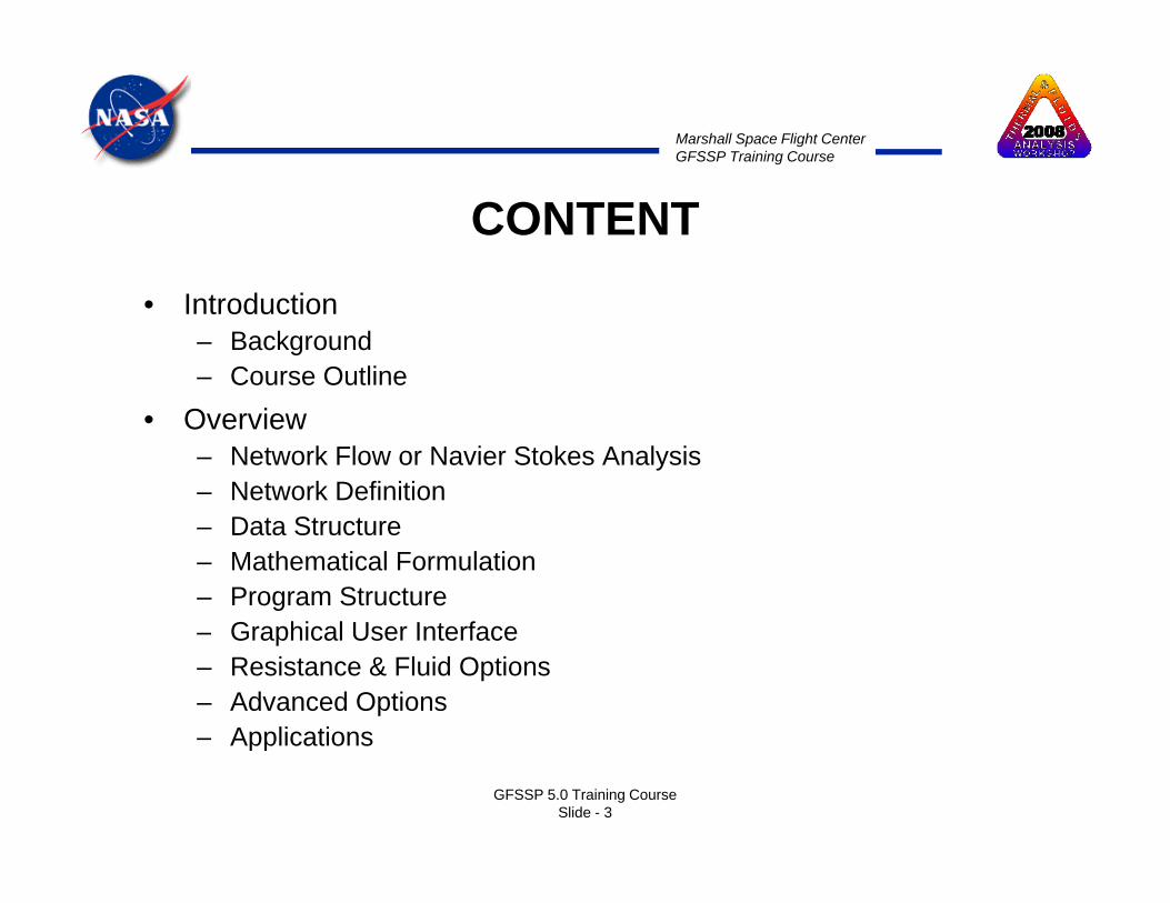
CONTENT• Introduction
– Background– Course Outline
• Overview– Network Flow or Navier Stokes Analysis– Network Definition – Data Structure– Mathematical Formulation – Program Structure
G hi l U I t f– Graphical User Interface– Resistance & Fluid Options– Advanced Options
Applications
GFSSP 5.0 Training CourseSlide - 3
– Applications
Marshall Space Flight CenterGFSSP Training Course
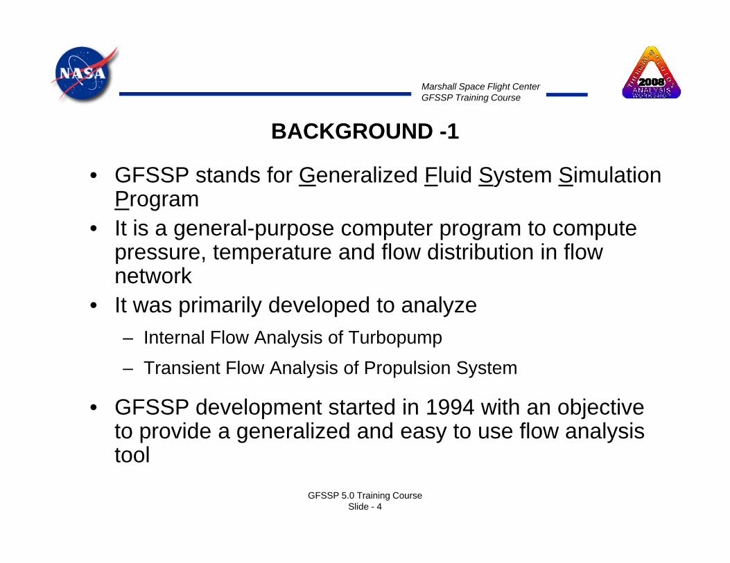
BACKGROUND -1
• GFSSP stands for Generalized Fluid System Simulation• GFSSP stands for Generalized Fluid System Simulation Program
• It is a general-purpose computer program to compute t t d fl di t ib ti i flpressure, temperature and flow distribution in flow
network• It was primarily developed to analyze
– Internal Flow Analysis of Turbopump– Transient Flow Analysis of Propulsion System
• GFSSP development started in 1994 with an objective to provide a generalized and easy to use flow analysis tool
GFSSP 5.0 Training CourseSlide - 4
tool

Marshall Space Flight CenterGFSSP Training Course
BACKGROUND -2
DEVELOPMENT HISTORY
• Version 1.4 (Steady State) was released in 1996V i 2 01 (Th d i T i t) l d• Version 2.01 (Thermodynamic Transient) was released in 1998
• Version 3.0 (User Subroutine) was released in 1999e s o 3 0 (Use Sub ou e) as e eased 999• Graphical User Interface, VTASC was developed in
2000• Selected for NASA Software of the Year Award in 2001• Version 4.0 (Fluid Transient and post-processing
capability) is released in 2003GFSSP 5.0 Training Course
Slide - 5
capability) is released in 2003
Marshall Space Flight CenterGFSSP Training Course
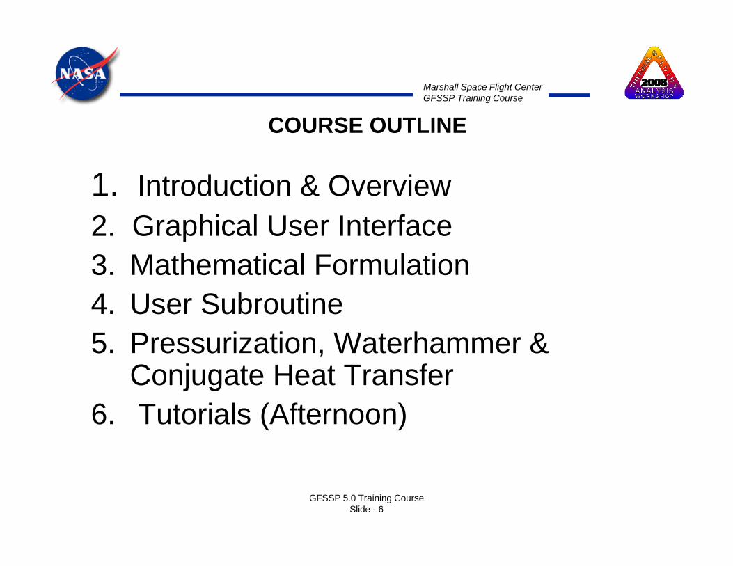
COURSE OUTLINE
1 I t d ti & O i1. Introduction & Overview2. Graphical User Interface3. Mathematical Formulation4. User Subroutine5. Pressurization, Waterhammer &
Conjugate Heat Transferj g6. Tutorials (Afternoon)
GFSSP 5.0 Training CourseSlide - 6

Marshall Space Flight CenterGFSSP Training Course
NETWORK FLOW OR NAVIER STOKES ANALYSIS - 1
Computational Fluid Dynamics (CFD)
Navier Stokes Analysis (NSA)
Network Flow Analysis (NFA)Analysis (NSA) Analysis (NFA)
Fi iFi i Finite FiniteFinite Difference
Finite Element
Finite Volume
Finite Volume
Finite Difference
GFSSP
GFSSP 5.0 Training CourseSlide - 7

Marshall Space Flight CenterGFSSP Training Course
NETWORK FLOW OR NAVIER STOKES ANALYSIS - 2
Navier Stokes Analysis• Suitable for detailed flow
analysis within a component
Network Flow Analysis• Suitable for flow analysis of a
system consisting of severalanalysis within a component• Requires fine grid resolution to
accurately model transport processes
system consisting of several components
• Uses empirical laws of transport process
• Used after after preliminary design
• Used during preliminary design
GFSSP 5.0 Training CourseSlide - 8

Marshall Space Flight CenterGFSSP Training Course
NETWORK DEFINITION – 1GFSSP FLOW CIRCUIT
= Boundary Node
= Internal Node
O2
H2 + O2 +N2 Internal Node
= Branch
GFSSP calculates pressure, temperature,
H2
and concentrations at nodes and calculates flow rates through branches.
H2 + O2 +N2
branches.
GFSSP 5.0 Training CourseSlide - 9
N2
Marshall Space Flight CenterGFSSP Training Course
NETWORK DEFINITIONS - 2
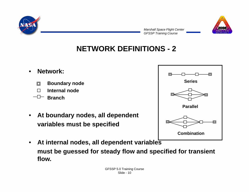
• Network:
Boundary node SeriesBoundary nodeInternal nodeBranch
Parallel
• At boundary nodes, all dependent variables must be specified
C bi ti
• At internal nodes, all dependent variables must be guessed for steady flow and specified for transient fl
Combination
GFSSP 5.0 Training CourseSlide - 10
flow.

Marshall Space Flight CenterGFSSP Training Course
NETWORK DEFINITIONS - 3
UNITS AND SIGN CONVENTIONS• Units External (input/output) Internal (inside GFSSP)
– Length - inches - feetg– Area - inches2 - feet2– Pressure - psia - psf– Temperature - °F - °R– Mass injection - lbm/sec - lbm/sec– Mass injection - lbm/sec - lbm/sec– Heat Source - Btu/s OR Btu/lbm- Btu/s OR Btu/lbm
• Sign Conventiong– Mass input to node = positive– Mass output from node = negative– Heat input to node = positive
Heat o tp t from node negati e
GFSSP 5.0 Training CourseSlide - 11
– Heat output from node = negative
Marshall Space Flight CenterGFSSP Training Course
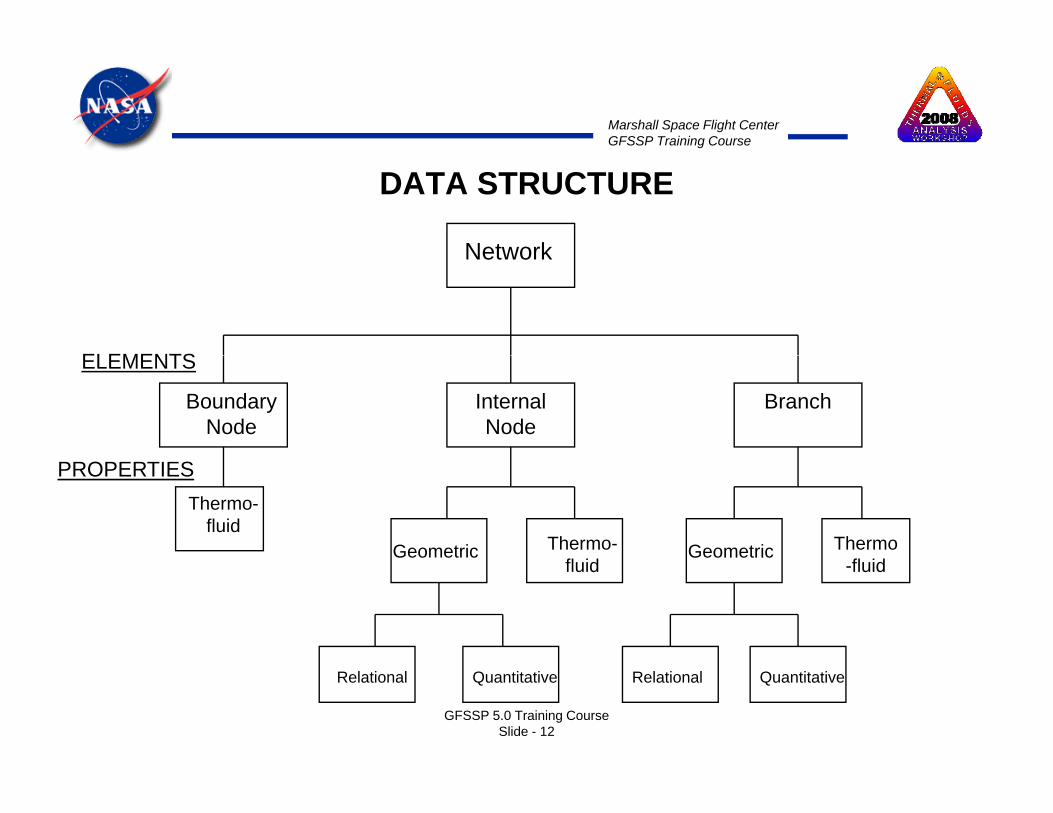
DATA STRUCTURE
NetworkNetwork
ELEMENTS
Boundary Node
Internal Node
Branch
ELEMENTS
Thermo-fluid
Geometric Thermo-fl id
Thermofl id
Geometric
PROPERTIES
fluid -fluid
GFSSP 5.0 Training CourseSlide - 12
Relational RelationalQuantitative Quantitative

Marshall Space Flight CenterGFSSP Training Course
MATHEMATICAL FORMULATION - 1MATHEMATICAL CLOSURE - 1
Principal Variables:
Unknown Variables Available Equations to Solveq
1. Pressure 1. Mass Conservation Equation
2 Flowrate 2 Momentum Conservation Equation2. Flowrate 2. Momentum Conservation Equation
3. Temperature 3. Energy Conservation Equation (First or Second Lawof Thermodynamics)
4. Specie Concentrations 4. Conservation Equations for Mass Fraction of Species
5 Mass 5 Thermodynamic Equation of State
GFSSP 5.0 Training CourseSlide - 13
5. Mass 5. Thermodynamic Equation of State

Marshall Space Flight CenterGFSSP Training Course
MATHEMATICAL FORMULATION - 2
MATHEMATICAL CLOSURE -2
Auxiliary Variables:yThermodynamic Properties & Flow Resistance Factor
Unknown Variables Available Equations to Solve
DensitySpecific Heats Equilibrium Thermodynamic RelationsViscosity [GASP, WASP & GASPAK Property Programs]y [ , p y g ]Thermal ConductivityFlow Resistance Factor Empirical Relations
GFSSP 5.0 Training CourseSlide - 14
Marshall Space Flight CenterGFSSP Training Course
MATHEMATICAL FORMULATION - 3
BOUNDARY CONDITIONS
• Governing equations can generate an infinite numberGoverning equations can generate an infinite number of solutions
A i l ti i bt i d ith i t f• A unique solution is obtained with a given set of boundary conditions
• User provides the boundary conditions
GFSSP 5.0 Training CourseSlide - 15

Marshall Space Flight CenterGFSSP Training Course
MATHEMATICAL FORMULATION - 3A TYPICAL FLOW CIRCUIT
16
Notes:1) Number of Internal Nodes = 72) Number of Branches = 123) Total Number of Equations = 7 x 4 + 12 = 40
Atmosphere14.7 psia
A TYPICAL FLOW CIRCUIT
25
87
47
86
4) Number of Equations Solved by Newton Raphson Method = 7 + 12 = 195) Number of Equations Solved by Successive Substitution Method = 3 x 7 = 21
Helium151 psia 87 86
46
88137
66
50
Atmosphere14.7 psia
151 psia70 o F
XX Branch
Legend
63
129138
67
25
49
58
142
Oxygen
Hydrogen172 psia-174 o F
X
X
Boundary Node
Internal Node
Assumed Branch Flow Direction
GFSSP 5.0 Training CourseSlide - 16
23 23 22606848
Oxygen550 psia-60 o F

Marshall Space Flight CenterGFSSP Training Course
PROGRAM STRUCTURE
Graphical User Interface (VTASC)
Solver & Property Module User Subroutines
(VTASC)
Input Data
New Physics
• Time dependent
process
• Equation Generator
• Equation Solver
• Fluid Property Program
Fileprocess
• non-linear boundary
conditions
• External source term• Creates Flow Circuit
• Runs GFSSP te a sou ce te
• Customized output
• New resistance / fluid
option
Output Data FileRuns GFSSP
• Displays results graphically
GFSSP 5.0 Training CourseSlide - 17
p

Marshall Space Flight CenterGFSSP Training Course
GRAPHICAL USER INTERFACE - 1MODEL BUILDING
GFSSP 5.0 Training CourseSlide - 18
Marshall Space Flight CenterGFSSP Training Course
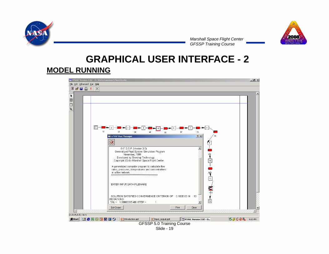
GRAPHICAL USER INTERFACE - 2MODEL RUNNING
GFSSP 5.0 Training CourseSlide - 19

Marshall Space Flight CenterGFSSP Training Course
GRAPHICAL USER INTERFACE - 3MODEL RESULTS
GFSSP 5.0 Training CourseSlide - 20
Marshall Space Flight CenterGFSSP Training Course
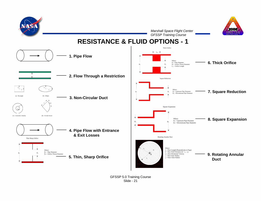
1. Pipe FlowWhere:D = Pipe Diameter
Lor
Thick Orifice
6 Thick Orifice
RESISTANCE & FLUID OPTIONS - 1
2. Flow Through a Restriction
bb
D2D1
D1 = Pipe DiameterD2 = Orifice Throat DiameterLor = Orifice Length
6. Thick Orifice
Square Reduction
b/2a
a
b
ba
(b) - Ellipse(a) - Rectangle
ba
3. Non-Circular Duct
D2D1
Where:D1 = Upstream Pipe DiameterD2 = Downstream Pipe Diameter 7. Square Reduction
Square Expansion
(d) - Circular Sector(c) - Concentric Annulus
4. Pipe Flow with Entrance& Exit Losses
Thin Sharp Orifice
8. Square ExpansionD1 D2
Where:D1 = Upstream Pipe DiameterD2 = Downstream Pipe Diameter
Rotating Annular Duct
D2D1
Where:D1 = Pipe DiameterD2 = Orifice Throat Diameter
Thin Sharp Orifice
5. Thin, Sharp Orifice 9. Rotating AnnularDuctri
ωro Where:
L = Duct Length (Perpendicular to Page)b = Duct Wall Thickness (b = ro - ri)ω = Duct Rotational Velocityri = Duct Inner Radiusro = Duct Outer Radius
GFSSP 5.0 Training CourseSlide - 21

Marshall Space Flight CenterGFSSP Training Course
RESISTANCE & FLUID OPTIONS -2Where:L = Duct Lengthω = Duct Rotational VelocityD = Duct Diameter
Rotating Radial Duct
D
13. Common Fittings10. Rotating Radial Duct
ω
L
Axis ofRotation
ri
rj
Labyrinth Seal
& Valves
14. Pump Characteristicsij
S
11. Labyrinth Sealri
CM
Where:C = ClearanceM = Gap Length (Pitch)ri = Radius (Tooth Tip)N = Number of Teeth
S
15. Pump Poweri
j
S
12. Face Seal
Where:c = Seal Thickness (Clearance)B = Passage Width (B = πD)L = Seal Length D
c
L
Flow
16. Valve with Given CvCv
17. Viscojet
L
c
B
Flow 18. Control Valve
GFSSP 5.0 Training CourseSlide - 22
P

Marshall Space Flight CenterGFSSP Training Course
RESISTANCE & FLUID OPTIONS - 3
Index Fluid Index Fluid
GASP & WASPIndex Fluid Index Fluid
1 HELIUM 7 ARGON
2 METHANE 8 CARBON DIOXIDE
3 NEON 9 FLUORINE3 9
4 NITROGEN 10 HYDROGEN
5 CARBON MONOXIDE 11 WATER
6 OXYGEN 12 RP-1
GFSSP 5.0 Training CourseSlide - 23
Marshall Space Flight CenterGFSSP Training Course
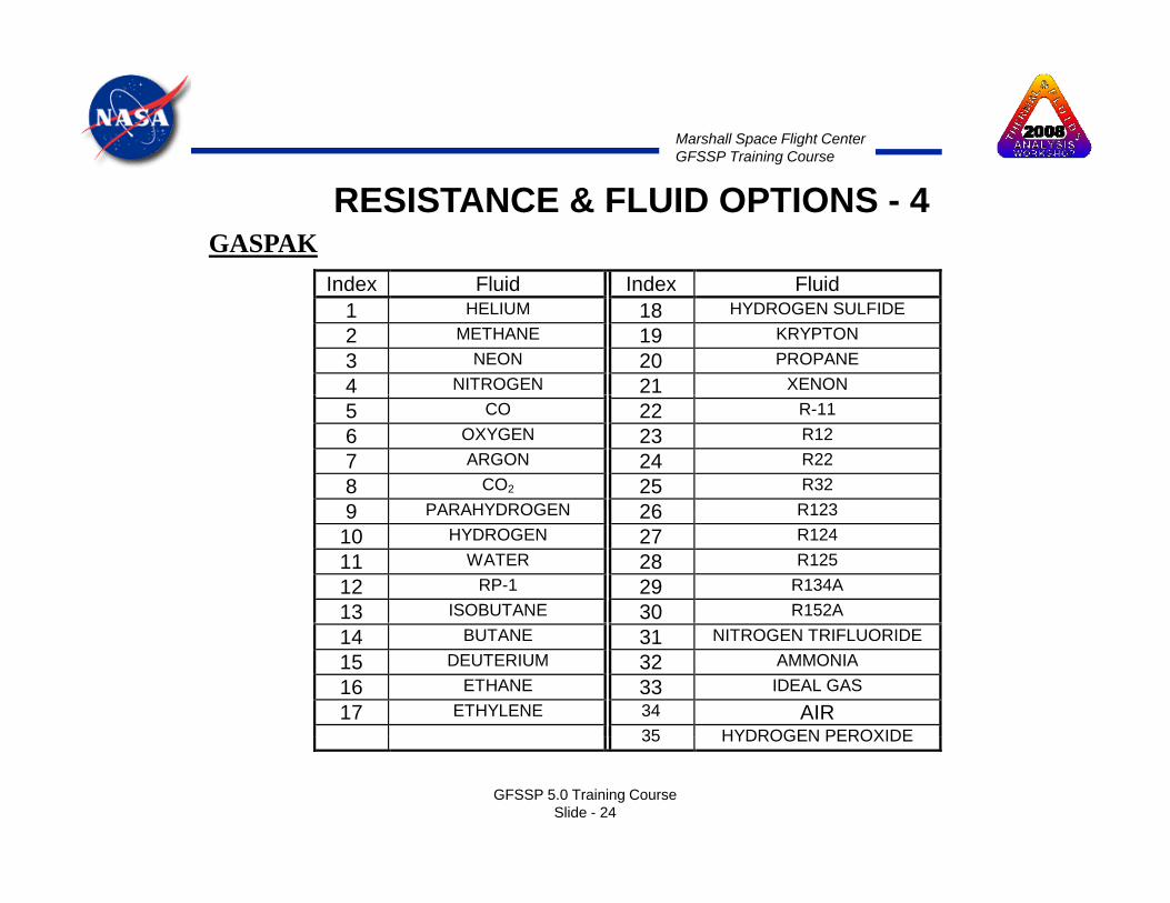
RESISTANCE & FLUID OPTIONS - 4
Index Fluid Index Fluid
GASPAKIndex Fluid Index Fluid
1 HELIUM 18 HYDROGEN SULFIDE 2 METHANE 19 KRYPTON 3 NEON 20 PROPANE 4 NITROGEN 21 XENON 5 CO 22 R-11 6 OXYGEN 23 R12 7 ARGON 24 R22 8 CO2 25 R32 9 PARAHYDROGEN 26 R1239 PARAHYDROGEN 26 R123
10 HYDROGEN 27 R124 11 WATER 28 R125 12 RP-1 29 R134A 13 ISOBUTANE 30 R152A 14 BUTANE 31 NITROGEN TRIFLUORIDE15 DEUTERIUM 32 AMMONIA 16 ETHANE 33 IDEAL GAS 17 ETHYLENE 34 AIR
35 HYDROGEN PEROXIDE
GFSSP 5.0 Training CourseSlide - 24
35 HYDROGEN PEROXIDE

Marshall Space Flight CenterGFSSP Training Course
ADDITIONAL OPTIONS
• Variable Geometry Option• Variable Rotation Optionp• Variable Heat Addition Option• Turbopump Optionp p p• Heat Exchanger• Tank PressurizationTank Pressurization• Control Valve
GFSSP 5.0 Training CourseSlide - 25

Marshall Space Flight CenterGFSSP Training Course
FASTRAC TURBOPUMPAPPLICATIONS - 1
GFSSP 5.0 Training CourseSlide - 26
Marshall Space Flight CenterGFSSP Training Course
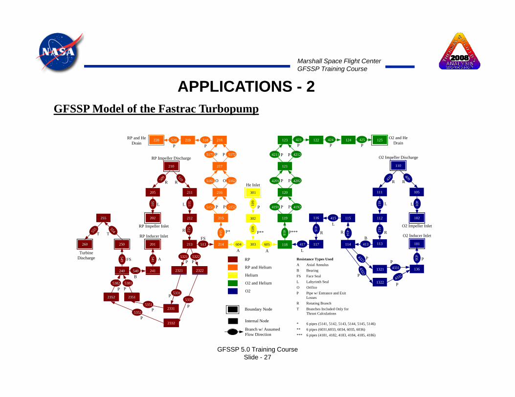
GFSSP Model of the Fastrac Turbopump
APPLICATIONS - 2
210 217
218
5171 5172
518219520220
110121
123
4211 4212
122423 124424 125425
RP Impeller Discharge
RP and HeDrain
O2 and HeDrain
O2 Impeller DischargeP P
P P P
P P
PP
115415116119
301
302
601
411
112215
511
212
216
5151 5152
5161 5162
510509
501
202
211205
409410
111 105
401
102
120
4191 4192
4201 4202
255
He Inlet
P P P
P P R R
L L
L
P P
O OR R
L L
RP
RP and Helium
H li
Resistance Types UsedA Axial AnnulusB Bearing
412
113114
414
416
117417
418
118
603
605303 413604214
514
513213
512
101
1321
4321
4322
201
241
541
540240
549
554555
250260
5382
2321 2322
5321 5322Turbine
Discharge
RP Impeller Inlet
RP Inducer Inlet
O2 Impeller Inlet
O2 Inducer InletP**
A A
P* P*** RRRB
PP
L
L
R
FS
FS P PA
T T
136
436 P
4331
Helium
O2 and Helium
O2
Boundary Node
Internal Node
FS Face SealL Labyrinth SealO OrificeP Pipe w/ Entrance and Exit
LossesR Rotating BranchT Branches Included Only for
Thrust Calculations
* 6 pipes (5141 5142 5143 5144 5145 5146)
1322
2
5382
2352 2351
2331
2332
5382 5381
5331
53515332
5352
P
PP P
B
P
P
P
P
4332
GFSSP 5.0 Training CourseSlide - 27
Branch w/ AssumedFlow Direction
* 6 pipes (5141, 5142, 5143, 5144, 5145, 5146)** 6 pipes (6031,6033, 6034, 6035, 6036)*** 6 pipes (4181, 4182, 4183, 4184, 4185, 4186)
2332

Marshall Space Flight CenterGFSSP Training Course
Turbopump Test to 20000 RPMTurbopump Test to 20000 RPMwith Gas Generatorwith Gas Generator
Turbopump Test to 20000 RPMTurbopump Test to 20000 RPMwith Gas Generatorwith Gas Generator
APPLICATIONS - 3
GFSSP 5.0 Training CourseSlide - 28
Marshall Space Flight CenterGFSSP Training Course
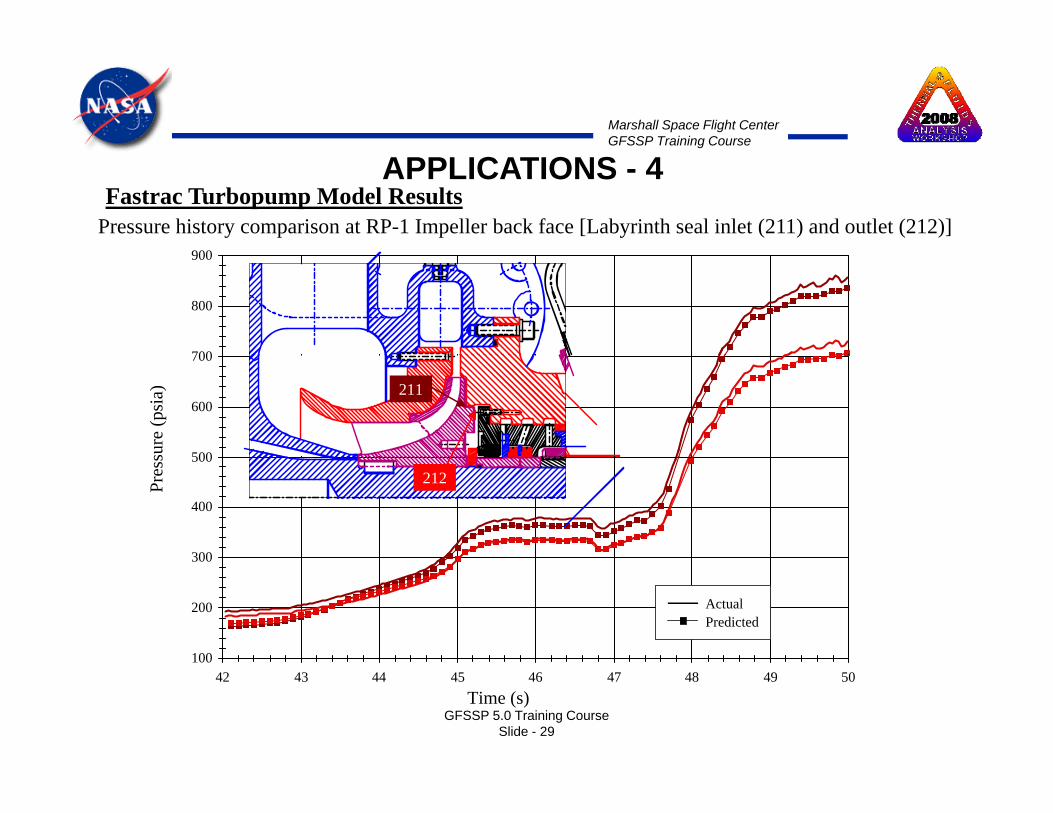
900
Pressure history comparison at RP-1 Impeller back face [Labyrinth seal inlet (211) and outlet (212)]
APPLICATIONS - 4Fastrac Turbopump Model Results
700
800
900
500
600
700
sure
(psi
a) 211
300
400
500
Pres
s
212
100
200
300
ActualPredicted
GFSSP 5.0 Training CourseSlide - 29
42 43 44 45 46 47 48 49 50Time (s)
Marshall Space Flight CenterGFSSP Training Course
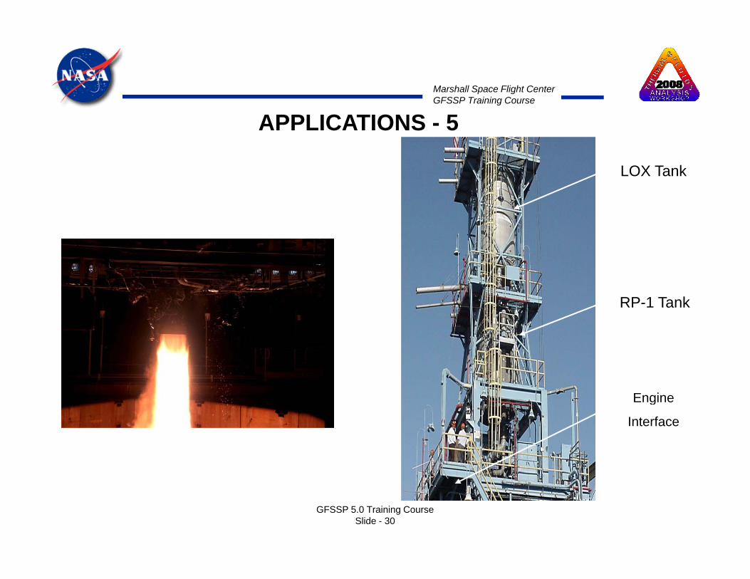
APPLICATIONS - 5
LOX Tank
RP-1 Tank
EngineEngine
Interface
GFSSP 5.0 Training CourseSlide - 30

Marshall Space Flight CenterGFSSP Training Course
APPLICATIONS - 6
1001 2 1002 3 1003 4 1004 5 1005 6 1006 7 1007 8 1008 9 1009 10 1010 11
PipeL=128 in.D=1.3 in.
PipeL=17 in.D=1.3 in.
PipeL=288 in.D=1.3 in.
PipeL=221 in.D=0.53 in.
PipeL 12 iPipe
Tee, Flo Thru K1=200 K2=0.1
Tee Flo Thru
Tee, Flo Thru K1=200 K2=0.1
SV7CL=0.6A=0.63617 in2
SV2
SV3CL=0.6A=0.63617 in2
SV4CL=0.6A=0.2827 in2Facility Interface
P=765 psia T=0-120 F
ReductionD1=1.3 in.D2=0.53 in.
Reduction
1
Tee, Flo Thru
GFSSP Model of PTA Helium Pressurization System
1011
1213 1012 1016 17
1013
14
1017
18
1034
3536 1035
1036
3738 1037 1041 42
1059
6062 611061 1060
1062
63
L=12 in.D=0.53 in.
PipeL=7.5 in.D=0.53 in.
PipeL=14 in.D=0.53 in.
PipePipe
PipeL=19 in.D=1.3 in.
Pipe
Tee, Flo Thru K1=200 K2=0.1
Tee, Elbow K1=500 K2=0.7
Tee, Elbow K1=500 K2=0.7
SV2CL=0.6A=0.63617 in2
SV5CL=0.6A=0.63617 in2
SV12SV13
ReductionD1=1.3 in.D2=0.78 in.
ReductionD1=1.3 in.D2=0.53 in.
, K1=200 K2=0.1
Tee, ElbowK1=500
Tee, ElbowK1=500 1014
15
1015
16
1018
19
1019
20211021 1020
1038
39
1039
40
1042
43
1043
44
1063
64
1064
PipeL=28 in.D=0.78 in.
pL=11 in.D=0.78 in.
PipeL=143 in.D=0.53 in.
Flex TubeL=28 in.D=0.53 in.
PipeL=9 in.D=0.53 in.
PipeL=14 in.D=0.53 in.
i Pipe
SV14CL=0.6A=0.63617 in2
SV15CL=0.6A=0.00001 in2
CL=0.6A=0.2827 in2
CL=0.6A=0.00001 in2
OF12CL=0.6A=0.02895 in2
FM1Engine Interface
65
Tee, Elbow
K1=500 K2=0.7
K1=500 K2=0.7
OF13CL=0.6A=0.00785 in2
OF15 1022
22
1024
24
231023
26 251026 1025
1040
41
1044
45461046 1045
1047
47 481048
PipeL=14 in.D=0.53 in.
PipeL=14 in.D=0.53 in.
PipePi
PipeL=18 in.D=0.78 in.
PipeL=15 in.D=0.78 in.
OF14CL=0.6A=0.10179 in2
FM2CL=0.77371A=0.55351 in2
FM1CL=0.83056A=0.2255 in2
CV9
CV8CL=0.6A=0.4185 in2
P=615 - 815 psia,
K1=500 K2=0.7
Tee, Elbow K1=500 K2=0.7
For stainless steel tubing, it is assumedthat ε=0.0008 in. For steel flex tubing,this roughness is multiplied by four.
ExpansionD1=0.53 in.D2=3.0 in.
Expansion
27 1027
Recovery
OF15CL=0.6A=0.01767 in2
V 285 f 31028
1049
49
1053
51 501051 1050
pL=13 in.D=0.78 in.
PipeL=21 in.D=0.78 in.
CV9CL=0.6A=0.7854 in2
LOX DiffuserC 0 6
RP1 DiffuserCL=0.6A=37.6991 in2
55
3028 1029
53 1054
ExpansionD1=0.78 in.D2=3.0 in.
1033
29
34
311030
54 561055 1056 59
LOX SurfaceC 0 0
RP1 SurfaceCL=0.0A=3987. in2
52 1052
RecoveryCL=0.0A=7.06858 in2
RecoveryCL=0.0A=7.06858 in2
Vull=25 ft3 Vprp=475 ft3
Vull=15 ft3 Vprp=285 ft3
321031 331032
57 1057 58 1058
RP1 Pump
LOX Pump Interface
LOX F dli
RP1 FeedlineCL = dependent on stage of operationA=14.25 in2
• Propellant Tanks
• Control Valves
GFSSP 5.0 Training CourseSlide - 31
CL=0.6A=37.6991 in2
CL=0.0A=4015. in2
RP1 Pump InterfaceLOX Feedline
CL = dependent on stage of operationA=14.25 in2
• Choked Orifices
• Various fittings

Marshall Space Flight CenterGFSSP Training Course
80
Comparison of LOX Ullage Pressure with Test Data
APPLICATIONS - 7
60
70
80
40
50
60
ure
(psi
a)
Engine Cut
20
30
Pres
su
GFSSPTest 31
0
10
GFSSP 5.0 Training CourseSlide - 32
-500 -400 -300 -200 -100 0 100 200
Tim e (sec)
Marshall Space Flight CenterGFSSP Training Course
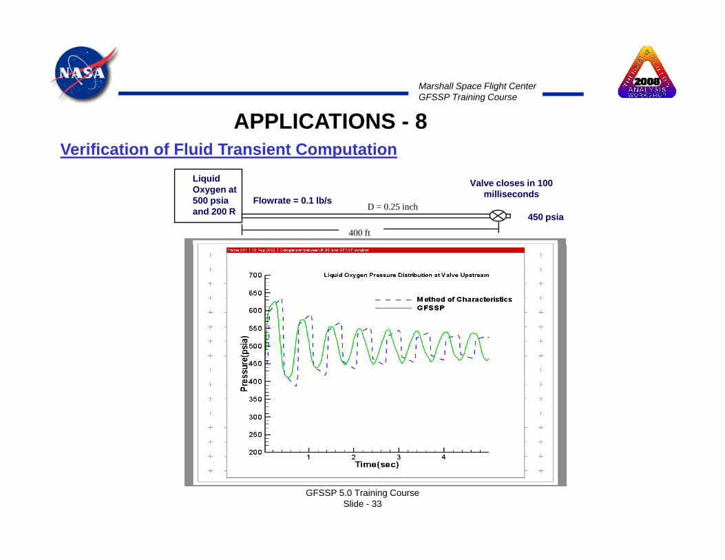
Verification of Fluid Transient ComputationAPPLICATIONS - 8
400 ft
D = 0.25 inch
Liquid Oxygen at 500 psia and 200 R
Flowrate = 0.1 lb/s
Valve closes in 100 milliseconds
450 psia
GFSSP 5.0 Training CourseSlide - 33

Marshall Space Flight CenterGFSSP Training Course
Fluid Transient in Two phase flow
APPLICATIONS - 9
GFSSP 5.0 Training CourseSlide - 34
Marshall Space Flight CenterGFSSP Training Course
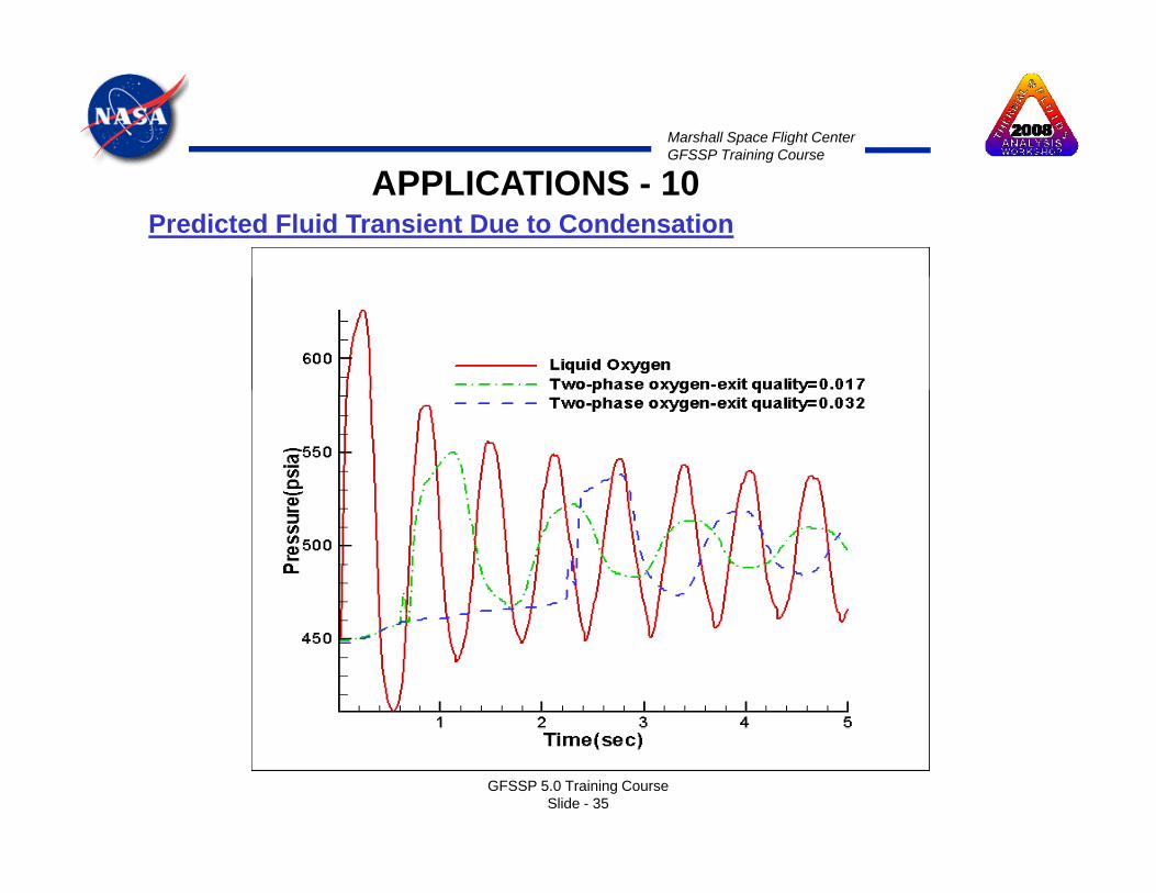
Predicted Fluid Transient Due to CondensationAPPLICATIONS - 10
GFSSP 5.0 Training CourseSlide - 35

Marshall Space Flight CenterGFSSP Training Course
SUMMARY - 1
• GFSSP is a finite volume based Network FlowGFSSP is a finite volume based Network Flow Analyzer
• Flow circuit is resolved into a network consisting of nodes and branchesnodes and branches
• Mass, energy and specie conservation are solved at internal nodes. Momentum conservation is solved at b hbranch
• Generalized data structure allows generation of all types of flow networkyp
• Modular code structure allows to add new capabilities with ease
GFSSP 5.0 Training CourseSlide - 36

Marshall Space Flight CenterGFSSP Training Course
SUMMARY – 2
• Unique mathematical formulation allows effective coupling of th d i d fl id h ithermodynamics and fluid mechanics
• Numerical scheme is robust; adjustment of numerical control parameters is seldom necessaryIntuitive Graphical User Interface makes it easy to build run and• Intuitive Graphical User Interface makes it easy to build, run and evaluate numerical models
• GFSSP has been successfully applied in various applications that includedthat included– Incompressible & Compressible flows– Phase change (Boiling & Condensation)– Fluid Mixture– Thermodynamic transient (Pressurization & Blowdown)– Fluid Transient (Waterhammer)– Conjugate Heat Transfer
GFSSP 5.0 Training CourseSlide - 37

Marshall Space Flight CenterGFSSP Training Course
SUMMARY – 3
• GFSSP is available from NASA/MSFC’s Technology Transfer Office for US Government agencies and contractors
• An Audio-Video Training Course is also il blavailable
• More information about the code and its th d l i il bl tmethodology is available at
http://mi.msfc.nasa.gov/GFSSP/index.shtml
GFSSP 5.0 Training CourseSlide - 38

VTASC – AN INTERACTIVE PREPROCESSOR FOR GFSSP
Marshall Space Flight CenterGFSSP Training Course
Marshall Space Flight CenterGFSSP Training Course
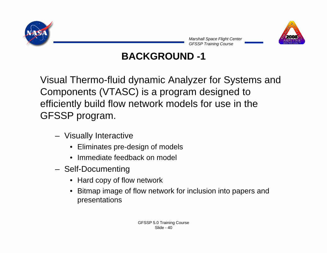
BACKGROUND -1
Visual Thermo fluid dynamic Analyzer for Systems andVisual Thermo-fluid dynamic Analyzer for Systems and Components (VTASC) is a program designed to efficiently build flow network models for use in the GFSSP program.
– Visually Interactive• Eliminates pre-design of models• Immediate feedback on model
– Self-Documenting• Hard copy of flow network• Bitmap image of flow network for inclusion into papers and
presentations
GFSSP 5.0 Training CourseSlide - 40

Marshall Space Flight CenterGFSSP Training Course
BACKGROUND -2
Eliminates errors during model building process– Eliminates errors during model building process• Automatic node and branch numbering• Save and restore models at any point in the model building
processprocess• Robust
– Pushbutton generation of GFSSP input file• Steady and Transient cases• Steady and Transient cases• Advanced features such as Turbopump, Tank Pressurization
and Heat ExchangersRun GFSSP directly from VTASC window– Run GFSSP directly from VTASC window
• GFSSP Run Manager acts as VTASC/GFSSP interface
GFSSP 5.0 Training CourseSlide - 41
Marshall Space Flight CenterGFSSP Training Course
BACKGROUND -3
– Post-processing capability allows quick study of results• Pushbutton access to GFSSP output file• Point and click access to output at each node and branchPoint and click access to output at each node and branch• Built-in plotting capability for transient cases• Capable of plotting through Winplot
– Cross platform operationCross platform operation• Program written in C++• Uses cross platform C++ GUI toolkit
GFSSP 5.0 Training CourseSlide - 42

Marshall Space Flight CenterGFSSP Training Course
CREATING A CHART IN WINPLOT -1
GFSSP 5.0 Training CourseSlide - 43
•After completing a model run, select Winplot from the VTASC Run Menu
Marshall Space Flight CenterGFSSP Training Course
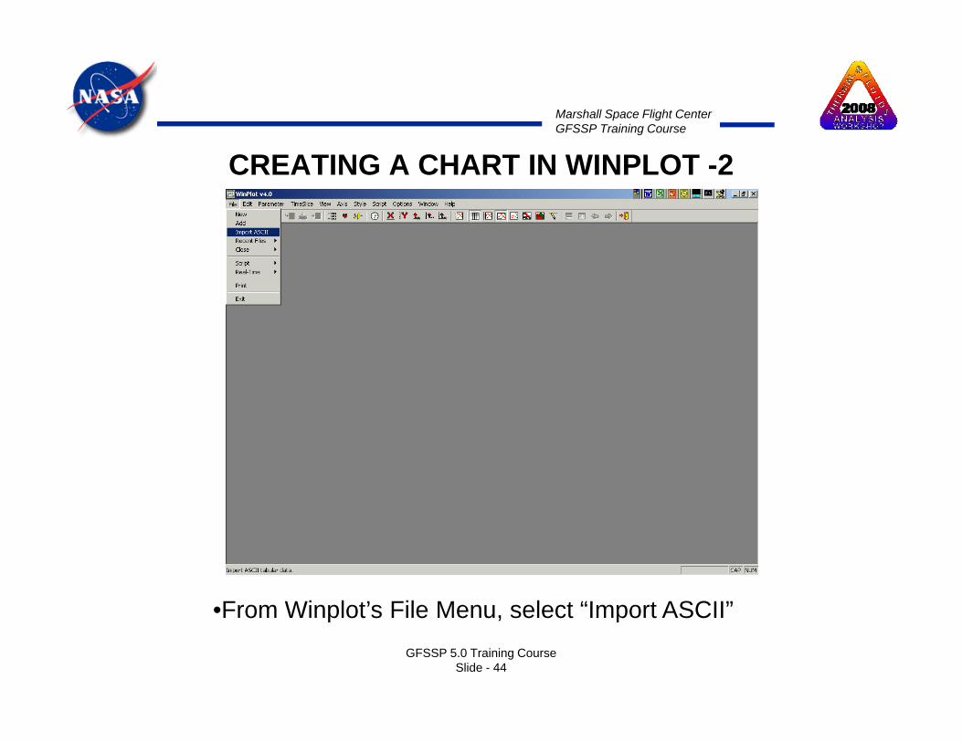
CREATING A CHART IN WINPLOT -2
From Winplot’s File Men select “Import ASCII”GFSSP 5.0 Training Course
Slide - 44
•From Winplot’s File Menu, select “Import ASCII”

Marshall Space Flight CenterGFSSP Training Course
CREATING A CHART IN WINPLOT -3
•Use the Browse window to select the files you wish to import•The default GFSSP Winplot files are “winpltb.csv” & “winpltn.csv”•Selecting a file opens the Importing window. Click Import.
GFSSP 5.0 Training CourseSlide - 45
g p p g p
Marshall Space Flight CenterGFSSP Training Course
CREATING A CHART IN WINPLOT -4
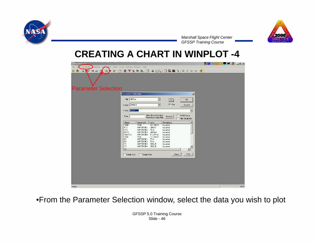
Parameter Selection
From the Parameter Selection indo select the data o ish to plotGFSSP 5.0 Training Course
Slide - 46
•From the Parameter Selection window, select the data you wish to plot
Marshall Space Flight CenterGFSSP Training Course
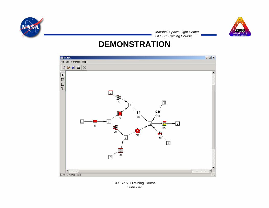
DEMONSTRATION
GFSSP 5.0 Training CourseSlide - 47

Marshall Space Flight CenterGFSSP Training Course
VTASC DEMONSTRATION PROBLEMS -1
Receiving Reservoir
150 ft Pipe
Flow150 ft
Supply ReservoirL = 1500 ftD = 6 in.ε/D = 0.005
Pipe
θ θ(WRT Gravity Vector) = 95.74°
PumpGateValve
WaterGravity Vector
GFSSP 5.0 Training CourseSlide - 48
Valve
Marshall Space Flight CenterGFSSP Training Course
VTASC DEMONSTRATION PROBLEMS -2
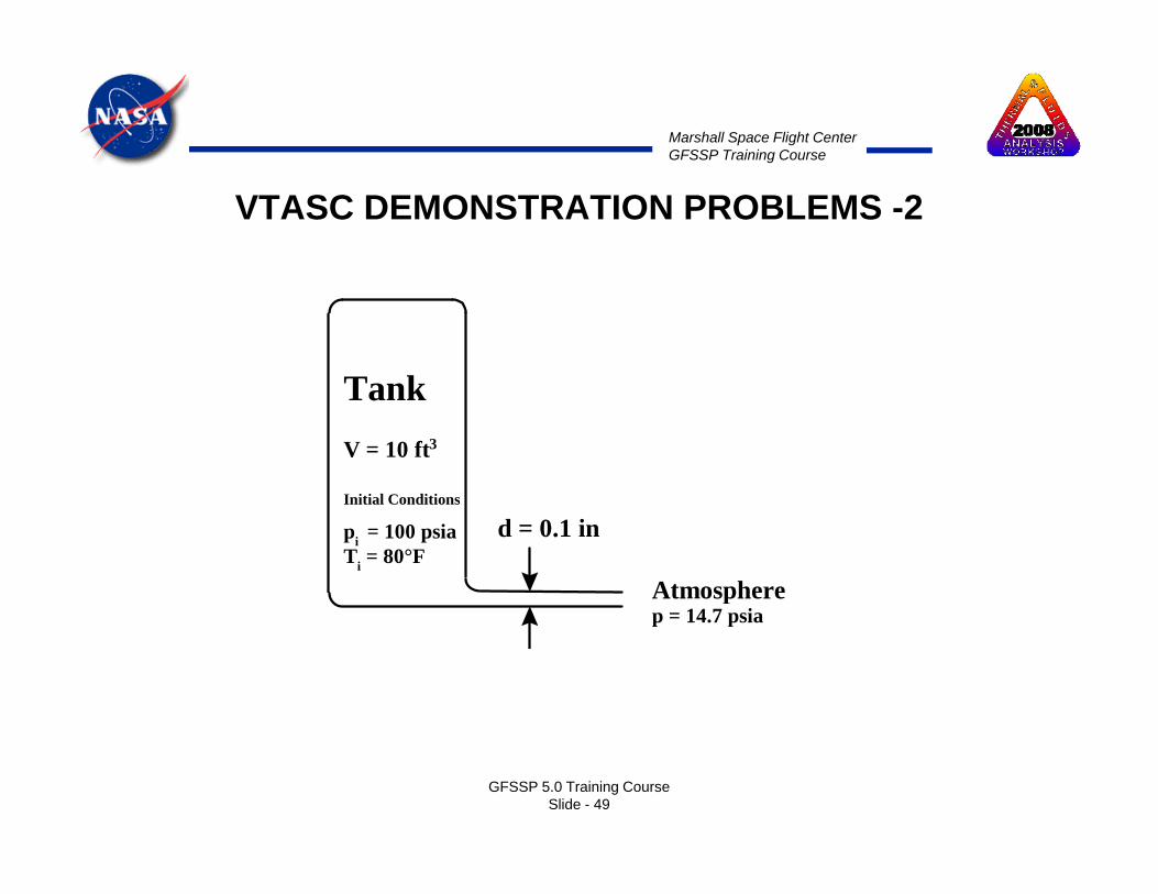
TankTankV = 10 ft3
Initial ConditionsInitial Conditions
pi = 100 psiaTi = 80°F
d = 0.1 in
Atmospherep = 14 7 psiap = 14.7 psia
GFSSP 5.0 Training CourseSlide - 49

Marshall Space Flight CenterGFSSP Training Course
VTASC DEMONSTRATION PROBLEMS -3
GFSSP 5.0 Training CourseSlide - 50

Marshall Space Flight CenterGFSSP Training Course
SUMMARY
• VTASC is a flow network model builder for use with GFSSPFl t k b d i d d difi d• Flow networks can be designed and modified interactively using a “Point and Click” paradigm
• Generates GFSSP Version 4.0 compatible input filesGenerates GFSSP Version 4.0 compatible input files
GFSSP 5.0 Training CourseSlide - 51
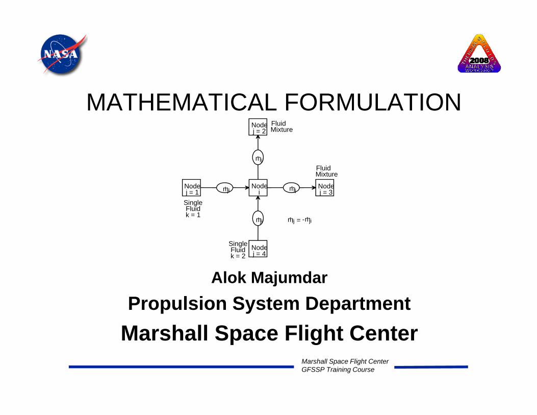
MATHEMATICAL FORMULATIONNodej 2
Fluid Mixturej = 2
mij.
Fluid Mixture
Mixture
Nodej = 1 mji
. Nodej = 3mij
.
mji. mji
.mij. = -
SingleFluidk = 1
Nodei
Alok Majumdar
Nodej = 4
SingleFluidk = 2
jPropulsion System Department
Marshall Space Flight CenterMarshall Space Flight CenterGFSSP Training Course
Marshall Space Flight Center
Marshall Space Flight CenterGFSSP Training Course
Content
• Mathematical Closure• Governing EquationsGoverning Equations• Solution Procedure
GFSSP 5.0 Training CourseSlide - 53
Marshall Space Flight CenterGFSSP Training Course
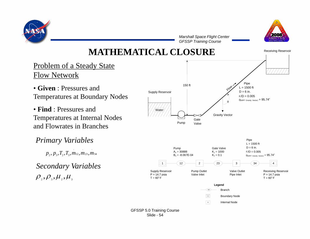
Receiving ReservoirMATHEMATICAL CLOSUREProblem of a Steady State Flow Network
Flow150 ft
Supply ReservoirL = 1500 ftD = 6 in.ε/D = 0.005
Pipe
θ θ(WRT Gravity Vector) = 95.74°
Flow Network
• Given : Pressures and Temperatures at Boundary Nodes
PumpGateValve
WaterGravity Vector
• Find : Pressures and Temperatures at Internal Nodes and Flowrates in Branches
1 212 23 3 34
PumpAo = 30888Bo = -8.067E-04
Gate ValveK1 = 1000K2 = 0.1
L = 1500 ftD = 6 in.ε/D = 0.005
Pipe
θ(WRT Gravity Vector) = 95.74°
4
Primary Variables34
.
23
.
12
.
3232 ,,,,,, mmmTTpp
S d V i blSupply ReservoirP = 14.7 psiaT = 60° F
Pump OutletValve Inlet
Valve OutletPipe Inlet
Receiving ReservoirP = 14.7 psiaT = 60° F
XX Branch
Legend
Secondary Variables3232
,,, μμρρ
GFSSP 5.0 Training CourseSlide - 54
X
X
Boundary Node
Internal Node
Marshall Space Flight CenterGFSSP Training Course
MATHEMATICAL CLOSUREProblem of an Unsteady Flow Network Primary Variables
• Given : Pressures and Temperatures at Boundary Nodes and Initial Values at Internal Nodes Secondary Variables
( ) ( ) ( ) ( )ττττ•
mmp T , , , 111
• Find : Pressures and Temperatures at Internal Nodes and Flowrates in Branches with Time.
( ) ( )τμτρ11
,
Tank3V = 10 ft3
Initial Conditions
pi = 100 psiaTi = 80°F
d = 0.1 in
1 212
Atmospherep = 14.7 psia
GFSSP 5.0 Training CourseSlide - 55

Marshall Space Flight CenterGFSSP Training Course
MATHEMATICAL CLOSURE
Principal Variables:Principal Variables:Unknown Variable Available Equations to Solve
1 Pressure 1 Mass Conservation Equation1. Pressure 1. Mass Conservation Equation
2. Flowrate 2. Momentum Conservation Equation
3 Temperature 3 Energy Conservation Equation3. Temperature 3. Energy Conservation Equation
4. Specie Concentrations 4. Conservation Equations for Mass Fraction of Species(Mixture)( )
5. Mass (Unsteady) 5. Thermodynamic Equation of State
GFSSP 5.0 Training CourseSlide - 56
Marshall Space Flight CenterGFSSP Training Course
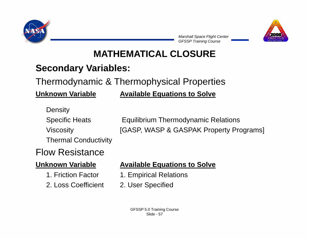
MATHEMATICAL CLOSURESecondary Variables:Thermodynamic & Thermophysical PropertiesUnknown Variable Available Equations to Solve
DensitySpecific Heats Equilibrium Thermodynamic RelationsViscosity [GASP, WASP & GASPAK Property Programs]Thermal Conductivity
Flow ResistanceUnknown Variable Available Equations to SolveUnknown Variable Available Equations to Solve
1. Friction Factor 1. Empirical Relations2. Loss Coefficient 2. User Specified
GFSSP 5.0 Training CourseSlide - 57

Marshall Space Flight CenterGFSSP Training Course
GOVERNING EQUATIONS
• Mass Conservation• Momentum Conservation• Energy Conservation• Fluid Species Conservation
E ti f St t• Equation of State• Mixture Property
GFSSP 5.0 Training CourseSlide - 58
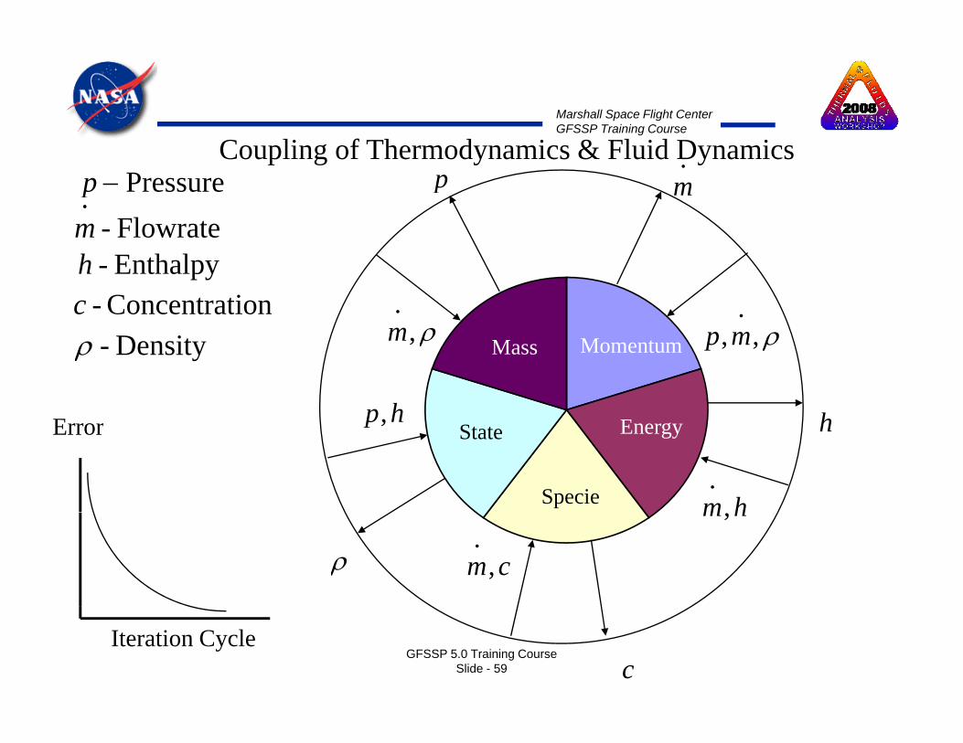
Marshall Space Flight CenterGFSSP Training Course
p.m Pressure−p
Flowrate-.m
Coupling of Thermodynamics & Fluid Dynamics
..
Flowrate- m Enthalpy- h
ionConcentrat - cMass Momentum ρ,,mpρ,m
hp hE
Density- ρ
Energy
Specie
Statehp,
hm.
hError
ρ
hm,
cm,.
GFSSP 5.0 Training CourseSlide - 59 c
Iteration Cycle
Marshall Space Flight CenterGFSSP Training Course
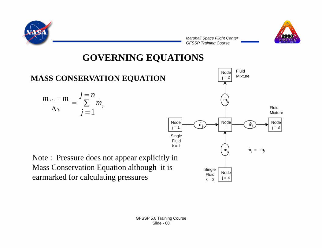
MASS CONSERVATION EQUATIONNodej = 2
Fluid Mixture
GOVERNING EQUATIONS
MASS CONSERVATION EQUATION j = 2
mij.
Fluid
Mixture
∑=
=Δ
−Δ+nj
mmmij
.
ττττ
Nodej = 1
mji. Node
j = 3mij.
SingleFl id
Fluid Mixture
Nodei
=Δ j 1τ
mji.
mji.
mij.
= -
Fluidk = 1
Single
Note : Pressure does not appear explicitly in Mass Conservation Equation although it is
Nodej = 4
gFluidk = 2
q gearmarked for calculating pressures
GFSSP 5.0 Training CourseSlide - 60

Marshall Space Flight CenterGFSSP Training Course
MOMENTUM CONSERVATION EQUATION jNode
GOVERNING EQUATIONS
.mij
Branch• Represents Newton’s Second Law of MotionMass X Acceleration = Forces
• Unsteady • Press re
i g
θ
Node
• Unsteady
• Longitudinal Inertia
• Transverse Inertia
• Pressure
• Gravity
• Friction
• Centrifugal
• Shear Stress
ω ri rjAxis of Rotation• Moving Boundary
• Normal Stress
• External Force
GFSSP 5.0 Training CourseSlide - 61
• External Force
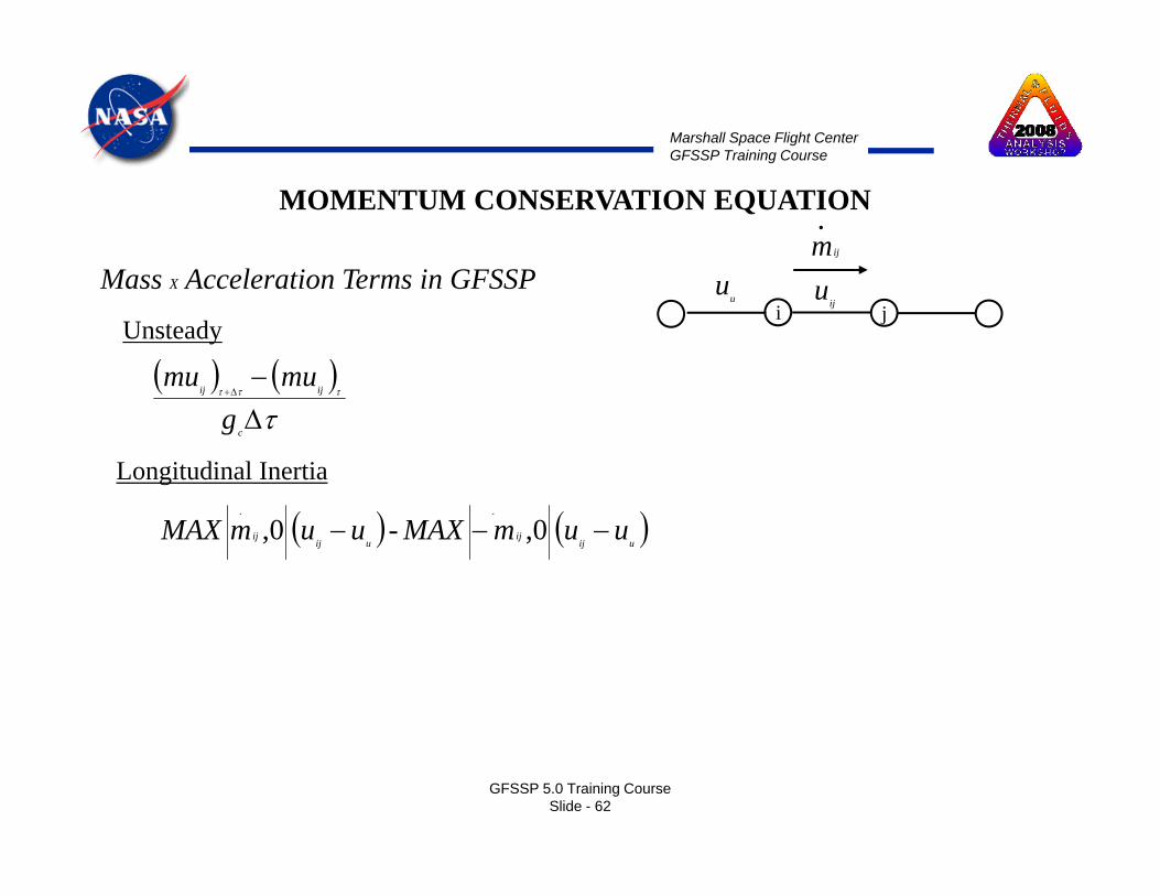
Marshall Space Flight CenterGFSSP Training Course
MOMENTUM CONSERVATION EQUATION
Mass Acceleration Terms in GFSSPijm
•
( ) ( )τττ
−Δ+ ijij
mumu
Mass X Acceleration Terms in GFSSP
Unsteadyi jij
uuu
( ) ( )τ
τττ
ΔΔ+
c
ijij
g
Longitudinal Inertia
( ) ( )uij
ijuij
ij uumMAXuumMAX −−− 0,- 0,..
GFSSP 5.0 Training CourseSlide - 62

Marshall Space Flight CenterGFSSP Training Course
MOMENTUM CONSERVATION EQUATION
Force Terms in GFSSP jNode
Pressure
G it
.mij
Branch
( )ijji App −
Gravity
i g
θ
Node
cg
gVCosθρ
Friction
C t if l
ijijij
fAmmK
••
−
Centrifugal ω ri rjAxis of Rotation
c
rot
gAK ωρ 22
GFSSP 5.0 Training CourseSlide - 63
Marshall Space Flight CenterGFSSP Training Course
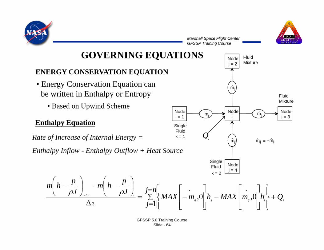
ENERGY CONSERVATION EQUATION
Nodej = 2
Fluid Mixture
GOVERNING EQUATIONS
mij.
Fluid Mixture
• Energy Conservation Equation can be written in Enthalpy or Entropy
• Based on Upwind SchemeNodej = 1 mji
. Nodej = 3
mij.
mji. mji
.mij.
= -
SingleFluidk = 1
Nodei
iQ
Enthalpy Equation
Rate of Increase of Internal Energy =
p
k 2
Nodej = 4
mji mjimij = -
SingleFluid
f f gy
Enthalpy Inflow - Enthalpy Outflow + Heat Source
k = 2j
Qnj
jhmMAXhmMAXJ
phmJphm
iiijjij+
=
= ⎪⎭
⎪⎬⎫
⎪⎩
⎪⎨⎧
⎥⎥⎦
⎤
⎢⎢⎣
⎡−
⎥⎥⎦
⎤
⎢⎢⎣
⎡−=
Δ
⎟⎠
⎞⎜⎝
⎛ −−⎟⎠
⎞⎜⎝
⎛ −∑Δ+
10,
.0,
.
τρρ
τττ
GFSSP 5.0 Training CourseSlide - 64
j= ⎪⎭⎪⎩ ⎥⎦⎢⎣⎥⎦⎢⎣Δ 1τ

Marshall Space Flight CenterGFSSP Training Course
ENERGY CONSERVATION EQUATION
Nodej = 2
Fluid Mixture
GOVERNING EQUATIONS
mij.
Fluid Mixture
Entropy Equation
Rate of Increase of Entropy =Nodej = 1 mji
. Nodej = 3
mij.
mji. mji
.mij.
= -
SingleFluidk = 1
Nodei
Rate of Increase of Entropy
Entropy Inflow - Entropy Outflow +
Entropy Generation + Entropy Source TQ /
k 2
Nodej = 4
mji mjimij = -
SingleFluid
iiTQ /
k = 2j
( ) ( ) [ ] [ ] [ ]
1 ,
.0,
10,0, ∑
=
=+
⎭⎬⎫
⎩⎨⎧ −
∑=
=+
⎭⎬⎫
⎩⎨⎧ −−=
Δ−Δ+ nj
j iT
iQ
genijSm
mMAXnj
j ismMAX
jsmMAX
msms
ij
ij
ijij&
&&&
ττττ
GFSSP 5.0 Training CourseSlide - 65
Marshall Space Flight CenterGFSSP Training Course
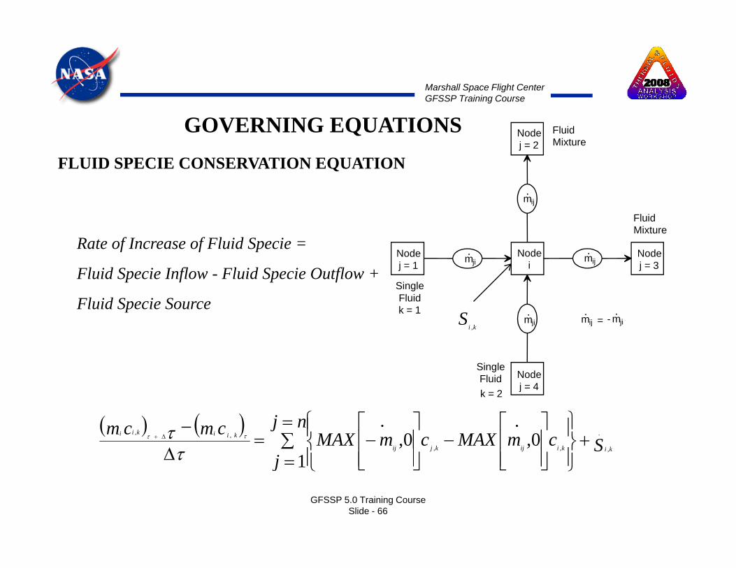
FLUID SPECIE CONSERVATION EQUATION
Nodej = 2
Fluid Mixture
GOVERNING EQUATIONS
mij.
Fluid Mixture
Rate of Increase of Fluid Specie =Nodej = 1 mji
. Nodej = 3
mij.
mji. mji
.mij.
= -
SingleFluidk = 1
Nodei
Rate of Increase of Fluid Specie
Fluid Specie Inflow - Fluid Specie Outflow +
Fluid Specie SourceS
k 2
Nodej = 4
mji mjimij = -
SingleFluid
kiS
,
k = 2j
( ) ( ) .
,,,
,,
10,
.0,
.S
nj
jcmMAXcmMAXcmcm
kikiijkjij
kiikii +∑=
= ⎪⎭
⎪⎬⎫
⎪⎩
⎪⎨⎧
⎥⎥⎦
⎤
⎢⎢⎣
⎡−
⎥⎥⎦
⎤
⎢⎢⎣
⎡−=
Δ−
Δ+
ττ ττ
GFSSP 5.0 Training CourseSlide - 66
1j = ⎪⎭⎪⎩ ⎥⎦⎢⎣⎥⎦⎢⎣

Marshall Space Flight CenterGFSSP Training Course
GOVERNING EQUATIONSEQUATION OF STATEQ
For unsteady flow, resident mass in a control volume is calculated
from the equation of state for a real fluidfrom the equation of state for a real fluid
RTpVm=RTz
Z is the compressibility factor determined from
higher order equation of state
GFSSP 5.0 Training CourseSlide - 67

Marshall Space Flight CenterGFSSP Training Course
EQUATION OF STATE
GOVERNING EQUATIONS
• GFSSP uses two separate Thermodynamic Property Packages
GASP/WASP and GASPAK
• GASP/WASP uses modified Benedict, Webb & Rubin (BWR)
Equation of Stateq
• GASPAK uses “standard reference” equation from
• National Institute of Standards and Technology (NIST)
• International Union of Pure & Applied Chemistry (IUPAC)
• National Standard Reference Data Service of the USSR
GFSSP 5.0 Training CourseSlide - 68

Marshall Space Flight CenterGFSSP Training Course
GOVERNING EQUATIONS
Mixture Property RelationMixture Property Relation
Density
• Calculated from Equation of State of Mixture with Compressibility Factor• Calculated from Equation of State of Mixture with Compressibility Factor
TRzi
piii
i=ρ ∑
=
==
nk
k kkiRxR
1Tzi ii
• Compressibility Factor of Mixture is Mole average of Individual Components
∑=
=nk
kz
kxz pi
kz =∑=
=k
kkiz
1 T kRkkkz
ρ=
GFSSP 5.0 Training CourseSlide - 69
Marshall Space Flight CenterGFSSP Training Course
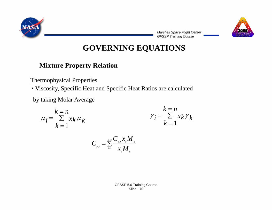
GOVERNING EQUATIONS
Mixture Property RelationMixture Property Relation
Thermophysical Properties• Viscosity, Specific Heat and Specific Heat Ratios are calculated
by taking Molar Average
∑=
=nk
kxki μμ ∑=
=nk
kxki γγ∑=
=k
kxki1
μμ
∑=
=nk
kkkpMxC
C ,
∑=k
kki1
γγ
∑=k
kk
ip MxC
1,
GFSSP 5.0 Training CourseSlide - 70
Marshall Space Flight CenterGFSSP Training Course
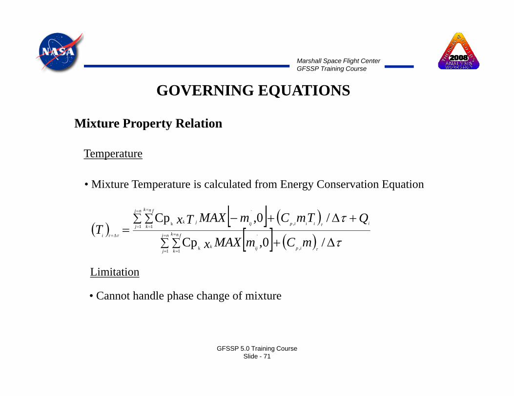
GOVERNING EQUATIONS
Mixture Property RelationMixture Property Relation
Temperature
• Mixture Temperature is calculated from Energy Conservation Equation
( )[ ] ( )∑ ∑
= =
+Δ+− iiiip
nj n fk
ijjk QTmCmMAXTx.
k/0,Cp τ
( )[ ] ( )
[ ] ( )∑ ∑
∑ ∑=
=
=
=
= =
Δ+
Δ+=
nj
j
n fk
k ipijk
iiiipj k ijjk
i
mCmMAXx
QTxT
1 1 ,
.
k
,1 1 k
/0,Cp
,p
ττ
τ
ττ
LimitationLimitation
• Cannot handle phase change of mixture
GFSSP 5.0 Training CourseSlide - 71
Marshall Space Flight CenterGFSSP Training Course
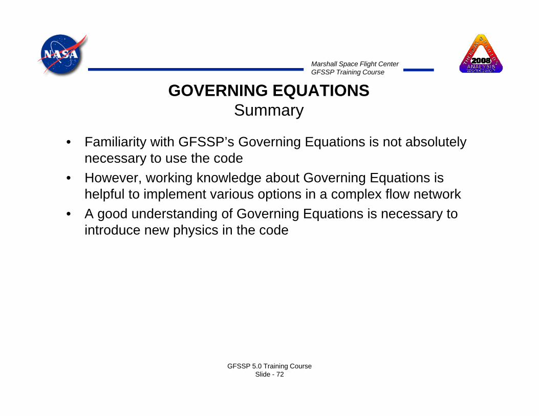
GOVERNING EQUATIONSSummary
• Familiarity with GFSSP’s Governing Equations is not absolutely necessary to use the code
• However, working knowledge about Governing Equations isHowever, working knowledge about Governing Equations is helpful to implement various options in a complex flow network
• A good understanding of Governing Equations is necessary to introduce new physics in the codeintroduce new physics in the code
GFSSP 5.0 Training CourseSlide - 72

Marshall Space Flight CenterGFSSP Training Course
SOLUTION PROCEDURE
• Successive Substitution• Newton-Raphson• Simultaneous Adjustment with Successive
Substitution (SASS)• Convergence• Convergence
GFSSP 5.0 Training CourseSlide - 73

Marshall Space Flight CenterGFSSP Training Course
SOLUTION PROCEDURE
• Non linear Algebraic Equations are solved by– Successive Substitution
Newton Raphson– Newton-Raphson
• GFSSP uses a Hybrid Method– SASS ( Simultaneous Adjustment with Successive ( j
Substitution)– This method is a combination of Successive Substitution and
Newton-Raphsonp
GFSSP 5.0 Training CourseSlide - 74
Marshall Space Flight CenterGFSSP Training Course
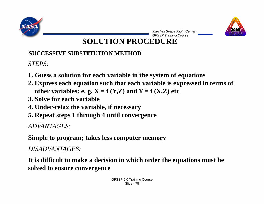
SUCCESSIVE SUBSTITUTION METHOD
STEPS:
SOLUTION PROCEDURE
STEPS:
1. Guess a solution for each variable in the system of equations2. Express each equation such that each variable is expressed in terms of
th i bl X f (Y Z) d Y f (X Z) tother variables: e. g. X = f (Y,Z) and Y = f (X,Z) etc3. Solve for each variable4. Under-relax the variable, if necessary5 Repeat steps 1 through 4 until convergence5. Repeat steps 1 through 4 until convergence
ADVANTAGES:
Simple to program; takes less computer memoryp p g ; p y
DISADVANTAGES:
It is difficult to make a decision in which order the equations must be l d t
GFSSP 5.0 Training CourseSlide - 75
solved to ensure convergence
Marshall Space Flight CenterGFSSP Training Course
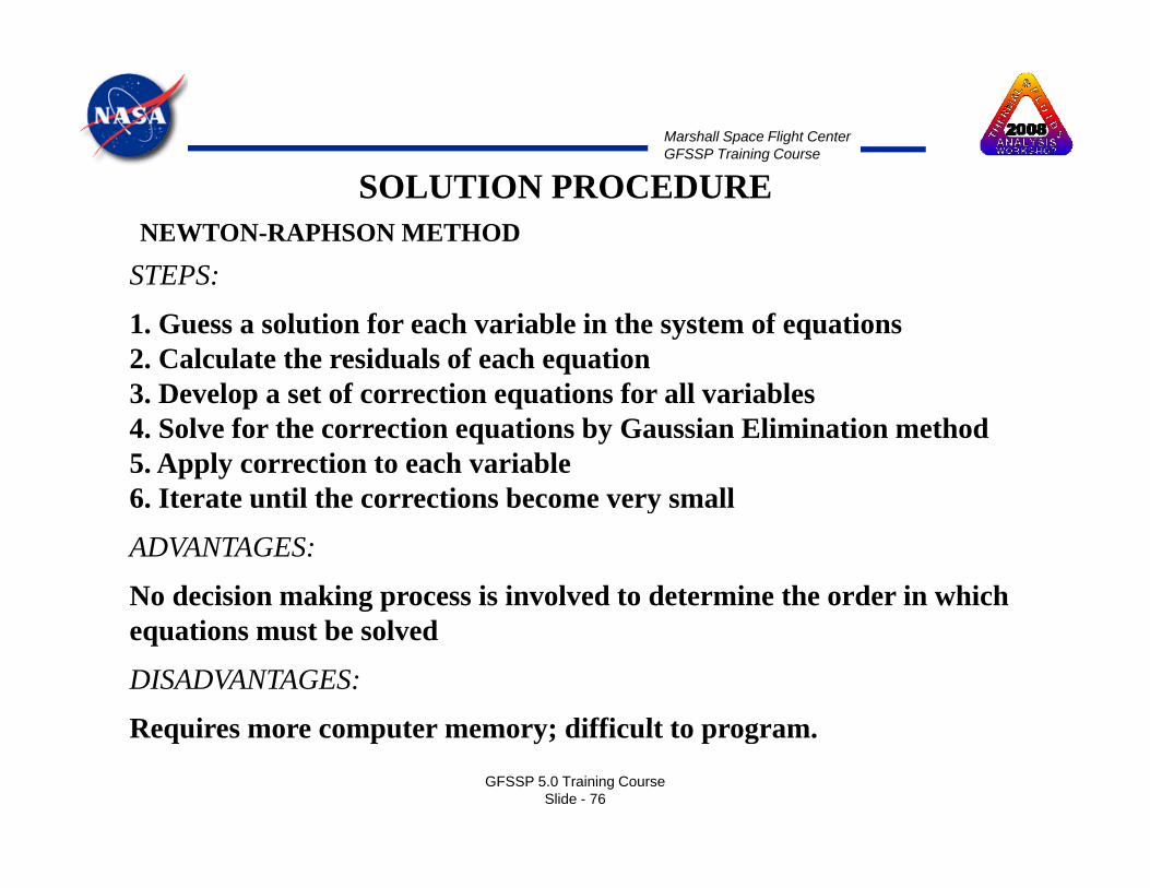
NEWTON-RAPHSON METHOD
STEPS:
SOLUTION PROCEDURE
STEPS:
1. Guess a solution for each variable in the system of equations2. Calculate the residuals of each equation3 D l t f ti ti f ll i bl3. Develop a set of correction equations for all variables4. Solve for the correction equations by Gaussian Elimination method5. Apply correction to each variable6 Iterate until the corrections become very small6. Iterate until the corrections become very small
ADVANTAGES:
No decision making process is involved to determine the order in which equations must be solved
DISADVANTAGES:
Req ires more comp ter memor ; diffic lt to program
GFSSP 5.0 Training CourseSlide - 76
Requires more computer memory; difficult to program.

Marshall Space Flight CenterGFSSP Training Course
SASS (Simultaneous Adjustment with Successive Substitution) SchemeSOLUTION PROCEDURE
• SASS is a combination of successive substitution and Newton-Raphsonmethod
• Mass conservation and flowrate equations are solved by Newton-Raphsonth dmethod
• Energy Conservation and concentration equations are solved bysuccessive substitution method
• Underlying principle for making such division:• Underlying principle for making such division:• Equations which have strong influences to other equations are solved
by the Newton-Raphson method• Equations which have less influence to other are solved by theq y
successive substitution method• This practice reduces code overhead while maintains superior
convergence characteristics
GFSSP 5.0 Training CourseSlide - 77
Marshall Space Flight CenterGFSSP Training Course
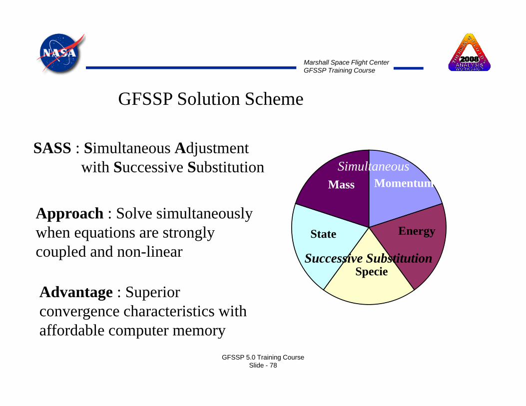
GFSSP Solution Scheme
SimultaneousSASS : Simultaneous Adjustment
with Successive SubstitutionMass Momentum
EApproach : Solve simultaneously
h ti t l Energy
Specie
State
Successive Substitution
when equations are strongly coupled and non-linear
Advantage : Superior convergence characteristics with affordable computer memory
GFSSP 5.0 Training CourseSlide - 78
affordable computer memory
Marshall Space Flight CenterGFSSP Training Course
CONVERGENCE
• Numerical solution can only be trusted when fully convergedGFSSP’ it i i b d• GFSSP’s convergence criterion is based on difference in variable values between successive iterations. Normalized Residual Error is also monitored
• GFSSP’s solution scheme has two options to control the iteration processthe iteration process– Simultaneous (SIMUL = TRUE)– Non-Simultaneous (SIMUL = FALSE)
GFSSP 5.0 Training CourseSlide - 79
Marshall Space Flight CenterGFSSP Training Course
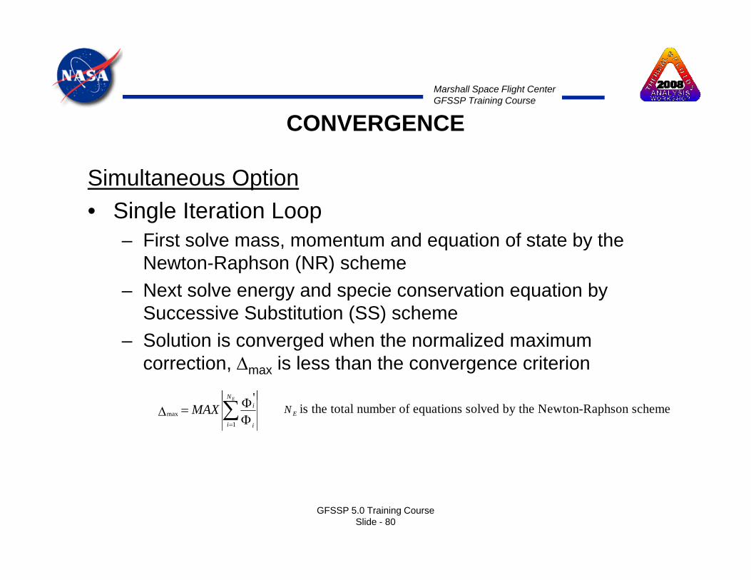
CONVERGENCE
Simultaneous OptionSimultaneous Option• Single Iteration Loop
– First solve mass, momentum and equation of state by the Newton-Raphson (NR) scheme
– Next solve energy and specie conservation equation by Successive Substitution (SS) scheme
– Solution is converged when the normalized maximum correction, Δmax is less than the convergence criterion
ΦEN '∑
= ΦΦ=Δ
E
i i
iMAX1
max EN is the total number of equations solved by the Newton-Raphson scheme
GFSSP 5.0 Training CourseSlide - 80
Marshall Space Flight CenterGFSSP Training Course
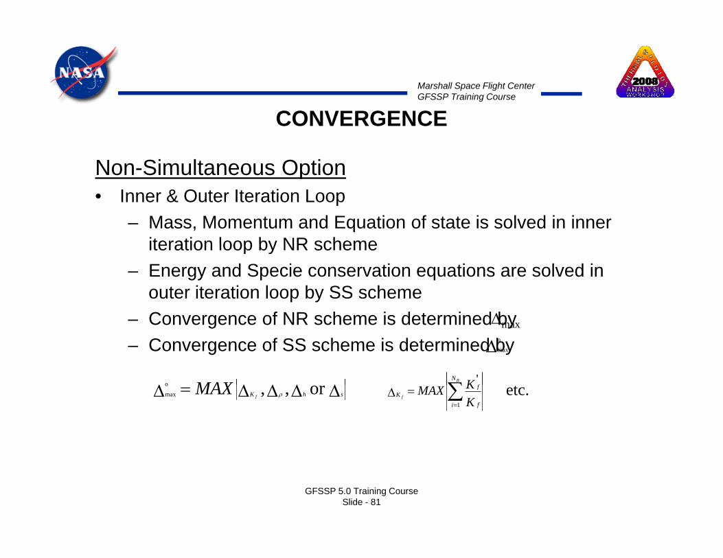
CONVERGENCE
Non-Simultaneous OptionNon Simultaneous Option• Inner & Outer Iteration Loop
– Mass, Momentum and Equation of state is solved in inner iteration loop by NR schemeiteration loop by NR scheme
– Energy and Specie conservation equations are solved in outer iteration loop by SS schemeC f NR h i d t i d bΔ– Convergence of NR scheme is determined by
– Convergence of SS scheme is determined by Δmax
Δomax
ΔΔΔΔΔ MAXo ∑BN
fK 'ΔΔΔΔ=Δ shK f
MAX or ,,omax ρ ∑
=
=Δ f
i f
fK
KKMAX
1
etc.
GFSSP 5.0 Training CourseSlide - 81

Marshall Space Flight CenterGFSSP Training Course
100
Convergence Characteristics For Simultaneous Option
Reduction of RSDMAX and DIFMAX with Iteration in
1
10Iterations
Example of Converging-Diverging Nozzle
0.1
10 5 10 15 20 25 30 35 40
0.001
0.01
RSDMAX
0.0001
DIFMAX
GFSSP 5.0 Training CourseSlide - 82
0.00001

Marshall Space Flight CenterGFSSP Training Course
100
Comparison of Convergence Characteristics between Simultaneous and Non-Simultaneous Option in Converging-Diverging Nozzle
1
10
0 20 40 60 80 100 120 140 160 180
RSDMAX Iterations
Simultaneous
0.01
0.1
0 00001
0.0001
0.001 Non-Simultaneous
0.0000001
0.000001
0.00001
GFSSP 5.0 Training CourseSlide - 83
0.00000001

Marshall Space Flight CenterGFSSP Training Course
SOLUTION PROCEDURESummary
• Simultaneous option is more efficient than Non-Simultaneous option
• Non-Simultaneous option is recommended when SimultaneousNon Simultaneous option is recommended when Simultaneous option experiences numerical instability
• Under-relaxation and good initial guess also help to overcome convergence problemconvergence problem
• A lack of realism in problem specification can lead to convergence problem
• Lack of realism includes:• Lack of realism includes:– Unrealistic geometry and/or boundary conditions– Attempt to calculate properties beyond operating range
GFSSP 5.0 Training CourseSlide - 84

USER SUBROUTINESUSER SUBROUTINESMAIN
C t l
FILENUMDefines input and output files numbers within the code
Solver Module/function User Subroutine/function
Controls programTSTEP
Allows user to overwrite the input deck defined time step
READINReads input data file
USRSETAllows user to redefine input file to custom format
INITProvides initial value
USRINTAll t it i iti l l dand steady state
boundary conditions
Allows user to overwrite initial values and steady state boundary conditions
BOUNDProvides time-dependant
boundary conditionsfrom history file
BNDUSERAllows user to define time-dependant boundary conditions
EQNS SORCEM
Alok Majumdar
EQNSGenerates mass &
momentum conservation equations along with
equation of resident mass
SORCEMAllows user to provide an external mass source
SORCEFAllows user to provide an external momentum source
jPropulsion System DepartmentMarshall Space Flight Center
Marshall Space Flight CenterGFSSP Training Course

Marshall Space Flight CenterGFSSP Training Course
CONTENT
• Motivation and Benefit
• How they work
GFSSP 5.0 Training CourseSlide - 86

Marshall Space Flight CenterGFSSP Training Course
MOTIVATION AND BENEFIT
• Motivation: To allow users to access GFSSP solver module to developGFSSP solver module to develop additional modeling capability
• Benefit: GFSSP users can work independently without Developer’s active involvementinvolvement
GFSSP 5.0 Training CourseSlide - 87

Marshall Space Flight CenterGFSSP Training Course
How do they work?- A series of subroutines are called from various locations of
solver module
The subroutines do not have any code but includes the- The subroutines do not have any code but includes the common block
- The users can write FORTRAN code to develop any new physical model in any particular node or branch
What users need to do?– Users need to compile a new file containing all user routines
and link that with GFSSP to create a new executable
GFSSP 5.0 Training CourseSlide - 88
Marshall Space Flight CenterGFSSP Training Course
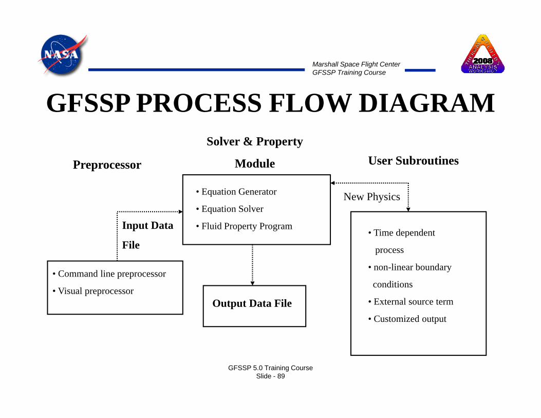
GFSSP PROCESS FLOW DIAGRAM
Preprocessor
Solver & Property
Module User Subroutines
Input Data
New Physics
• Time dependent
• Equation Generator
• Equation Solver
• Fluid Property Program
• Command line preprocessor
Vi l
FileTime dependent
process
• non-linear boundary
conditions• Visual preprocessor
• External source term
• Customized outputOutput Data File
GFSSP 5.0 Training CourseSlide - 89
Marshall Space Flight CenterGFSSP Training Course
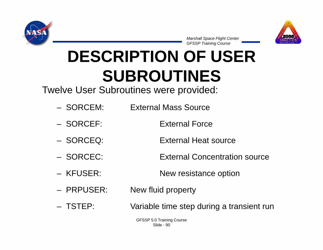
DESCRIPTION OF USER SUBROUTINESSUBROUTINES
Twelve User Subroutines were provided:
– SORCEM: External Mass SourceSORCEM: External Mass Source
– SORCEF: External Force
– SORCEQ: External Heat source– SORCEQ: External Heat source
– SORCEC: External Concentration source
KFUSER: New resistance option– KFUSER: New resistance option
– PRPUSER: New fluid property
TSTEP V i bl ti t d i t i tGFSSP 5.0 Training Course
Slide - 90
– TSTEP: Variable time step during a transient run

Marshall Space Flight CenterGFSSP Training Course
DESCRIPTION OF USER SUBROUTINESSUBROUTINES
– BNDUSER: Variable boundary condition during transient run (Alternative to history file)
– USRINT: Provide initial values and steady state boundary conditions
PRNUSER: Additional print out or creation of– PRNUSER: Additional print out or creation of additional file for post processing
– FILNUM: Assign file numbers; users can define new file numbers
– USRSET: User can supply all the necessary information by writing their own
GFSSP 5.0 Training CourseSlide - 91
information by writing their own code

Marshall Space Flight CenterGFSSP Training Course
MAINFILENUM
Defines input and output files numbers within the code
Solver Module/function User Subroutine/function
MAINControls program
TSTEPAllows user to overwrite the input deck defined time step
READIN USRSETReads input data file Allows user to redefine input file to custom format
INITProvides initial value
and steady stateboundary conditions
USRINTAllows user to overwrite initial values and
steady state boundary conditionsboundary conditions
BOUNDProvides time-dependant
boundary conditionsfrom history file
BNDUSERAllows user to define time-dependant boundary conditions
EQNSGenerates mass &
momentum conservation equations along with
equation of resident mass
SORCEMAllows user to provide an external mass source
SORCEF
GFSSP 5.0 Training CourseSlide - 92
equation of resident mass SORCEFAllows user to provide an external momentum source

Marshall Space Flight CenterGFSSP Training Course
Solver Module/function User Subroutine/function
ENTHALPY/ENTROPY SORCEQENTROPY
Generates and solves theenergy conservation
equation
QAllows user to provide an external heat source
MASSC SORCECGenerates and solves thespecie conservation
equation
SORCECAllows user to provide an external specie source
RESISTC l l t th fl
KFUSERCalculates the flow
resistance coefficient Allows user to define new resistance options
DENSITYCalculates the
PRPUSERAllows user to define new fluid properties
fluid properties
PRINTGenerates the Output files
PRNUSERAllows user to provide any additional output file(s)
GFSSP 5.0 Training CourseSlide - 93

Marshall Space Flight CenterGFSSP Training Course
GFSSP INDEXING SYSTEM• Node and Branch Variables are stored in one-
dimensional arrayN d i bl i l d• Node variables include:– Name– Pressure, Temperature, Concentration, Thermodynamic p y
properties
• Branch variables include:Name– Name
– Flowrate, Velocity, Resistance coefficients, Reynolds number
Th b ti d il bl t U fGFSSP 5.0 Training Course
Slide - 94
• Three subroutines are made available to Users for finding location and indices for a given node or branch
Marshall Space Flight CenterGFSSP Training Course
NODE & BRANCH INDEX• User defined node names are stored in NODE-array.
• NODE-array includes both internal and boundary y ynodes.
• Total number of elements in NODE-array is NNODES
• The internal nodes are stored in INODE-array.
• There are NINT elements in INODE array• There are NINT elements in INODE-array.
• Branch names are stored in IBRANCH-array
GFSSP 5.0 Training CourseSlide - 95
• There are NBR elements in IBRANCH-array
Marshall Space Flight CenterGFSSP Training Course
SUMMARY• User Subroutines can be used to add new capabilities that are
not available to Users through Logical Options
• New capabilities may include:• New capabilities may include:
– Introducing new type of resistance– Incorporating heat or mass transfer in any given node– Variable time step for a transient problem– Customized output
• Checklist for User SubroutinesChecklist for User Subroutines
– Identify subroutines that require modifications– Select GFSSP variables that require to be modified
Make use of GFSSP provided User variables in your coding
GFSSP 5.0 Training CourseSlide - 96
– Make use of GFSSP provided User variables in your coding
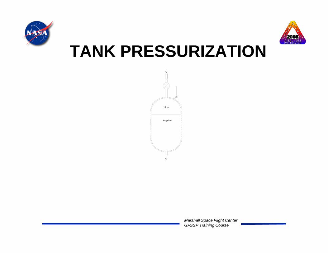
TANK PRESSURIZATIONTANK PRESSURIZATION
Ullage
P
Propellant
Marshall Space Flight CenterGFSSP Training Course

Marshall Space Flight CenterGFSSP Training Course
TANK PRESSURIZATIONPressurant
• Predict the ullage conditions considering Ullage.
WALLTTULLAGE
heat and mass transfer between the propellant and the tank wall
gQPROP
WALLQ.
QCOND
.
mPROP
. V
• Predict the propellant conditions leaving the t k
Propellant
TPROP
tank
GFSSP 5.0 Training CourseSlide - 98 Propellant to Engine

Marshall Space Flight CenterGFSSP Training Course
TANK PRESSURIZATIONADDITIONAL PHYSICAL PROCESSES
• Change in ullage and propellant volume.
• Change in gravitational head in the tank
Pressurant
WALLTT• Change in gravitational head in the tank.
• Heat transfer from pressurant to propellant.
• Heat transfer from pressurant to the tank
UllageQPROP
WALLQ..
WALL
QCOND
.
TULLAGE
mPROP
. V
• Heat transfer from pressurant to the tankwall.
• Heat conduction between the pressurant
Propellant
TPROP
PROP
exposed tank surface and the propellantexposed tank surface.
• Mass transfer between the pressurant and
GFSSP 5.0 Training CourseSlide - 99
Mass transfer between the pressurant andpropellant. Propellant to Engine

Marshall Space Flight CenterGFSSP Training Course
TANK PRESSURIZATIONCALCULATION STEPS
For each time step calculateUll d P ll t V l
Pressurant
WALLTTULLAGE• Ullage and Propellant Volumes
• Tank Bottom Pressure
UllageQPROP
WALLQ..
QCOND
.
ULLAGE
mPROP
. V
• Heat Transfer between pressurant and propellant and pressurant and wall
• Wall Temperature
Propellant
TPROP
• Wall Temperature
• Mass Transfer from propellant to ullage
GFSSP 5.0 Training CourseSlide - 100
Propellant to Engine

Marshall Space Flight CenterGFSSP Training Course
TANK PRESSURIZATION ADDITIONAL INPUT DATA FOR PRESSURIZATION
PRESS Logical Variable to Activate the OptionNTANK Number of Tanks in the CircuitNODUL Ullage Node
Pressurant
WALLTTULLAGENODUL Ullage Node
NODULB Pseudo Boundary Node at interfaceNODPRP Propellant NodeIBRPRP Branch number connecting NODULB & NODPRP
UllageQPROP
WALLQ..
QCOND
.
TULLAGE
mPROP
. V
TNKAR Tank Surface Area in Ullage at Start, in2
TNKTH Tank Thickness, inTNKRHO Tank Density, lbm/ft3
TNKCP Tank Specific Heat, Btu/lbm - R
Propellant
TPROP
TNKCP Tank Specific Heat, Btu/lbm RTNKCON Tank Thermal Conductivity, Btu/ft-sec-RARHC Propellant Surface Area, in2
FCTHC Multiplying Factor in Heat Transfer CoefficientTNKTM I iti l T k T t F
GFSSP 5.0 Training CourseSlide - 101
TNKTM Initial Tank Temperature, o FPropellant to Engine
Marshall Space Flight CenterGFSSP Training Course
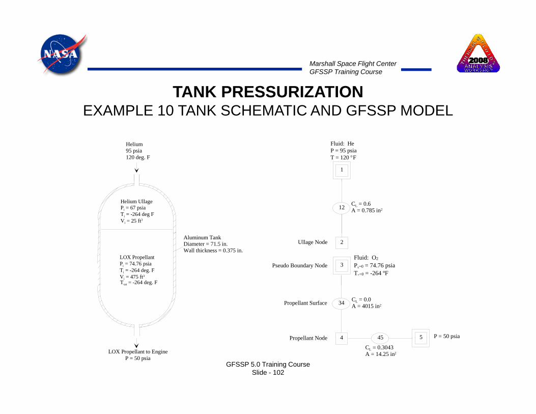
TANK PRESSURIZATIONEXAMPLE 10 TANK SCHEMATIC AND GFSSP MODEL
1
Fluid: HeP = 95 psiaT = 120 °F
Helium95 psia120 deg. F
12 CL = 0.6A = 0.785 in2
Helium UllagePi = 67 psiaTi = -264 deg FVi = 25 ft3
2
3Pseudo Boundary Node
Ullage Node
Fluid: O2
Pτ=0 = 74.76 psiaTτ=0 = -264 ºF
LOX PropellantPi = 74.76 psiaTi = -264 deg. FVi = 475 ft3
Aluminum TankDiameter = 71.5 in.Wall thickness = 0.375 in.
Tsat = -264 deg. F
4 45 5
34
P = 50 psiaPropellant Node
CL = 0.0A = 4015 in2Propellant Surface
GFSSP 5.0 Training CourseSlide - 102
4 45 5 P 50 psia
CL = 0.3043A = 14.25 in2
Propellant Node
LOX Propellant to Engine P = 50 psia

Marshall Space Flight CenterGFSSP Training Course
TANK PRESSURIZATIONEXAMPLE 10 PRESSURIZATION INPUT
NODE PRES (PSI) TEMP(DEGF) MASS SOURC HEAT SOURC THRST AREA VOLUME CONCENTRATION2 0.6700E+02 -0.2640E+03 0.0000E+00 0.0000E+00 0.0000E+00 0.4320E+05 1.0000 0.00004 0.7476E+02 -0.2640E+03 0.0000E+00 0.0000E+00 0.0000E+00 0.8208E+06 0.0000 1.0000
ex10h1.dat 10h3 d tex10h3.dat
ex10h5.dat ...
NUMBER OF TANKS IN THE CIRCUITNUMBER OF TANKS IN THE CIRCUIT1
NODUL NODULB NODPRP IBRPRP TNKAR TNKTH TNKRHOTNKCP TNKCON ARHC FCTHC TNKTM2 3 4 34 6431.91 0.375 170.00 0.20 0.0362 4015.00 1.00 -264.00
NODE DATA FILE FNODE.DAT Tank Input Units BRANCH DATA FILE
FBRANCH.DAT VOLUME, in3
TNKAR, in2
TNKTH, inTNKRHO, lbm/ft3
TNKCP, Btu/lbm-RTNKCON Btu/ft s R
GFSSP 5.0 Training CourseSlide - 103
TNKCON, Btu/ft-s-RARHC, in2
TNKTM, deg. F
Marshall Space Flight CenterGFSSP Training Course
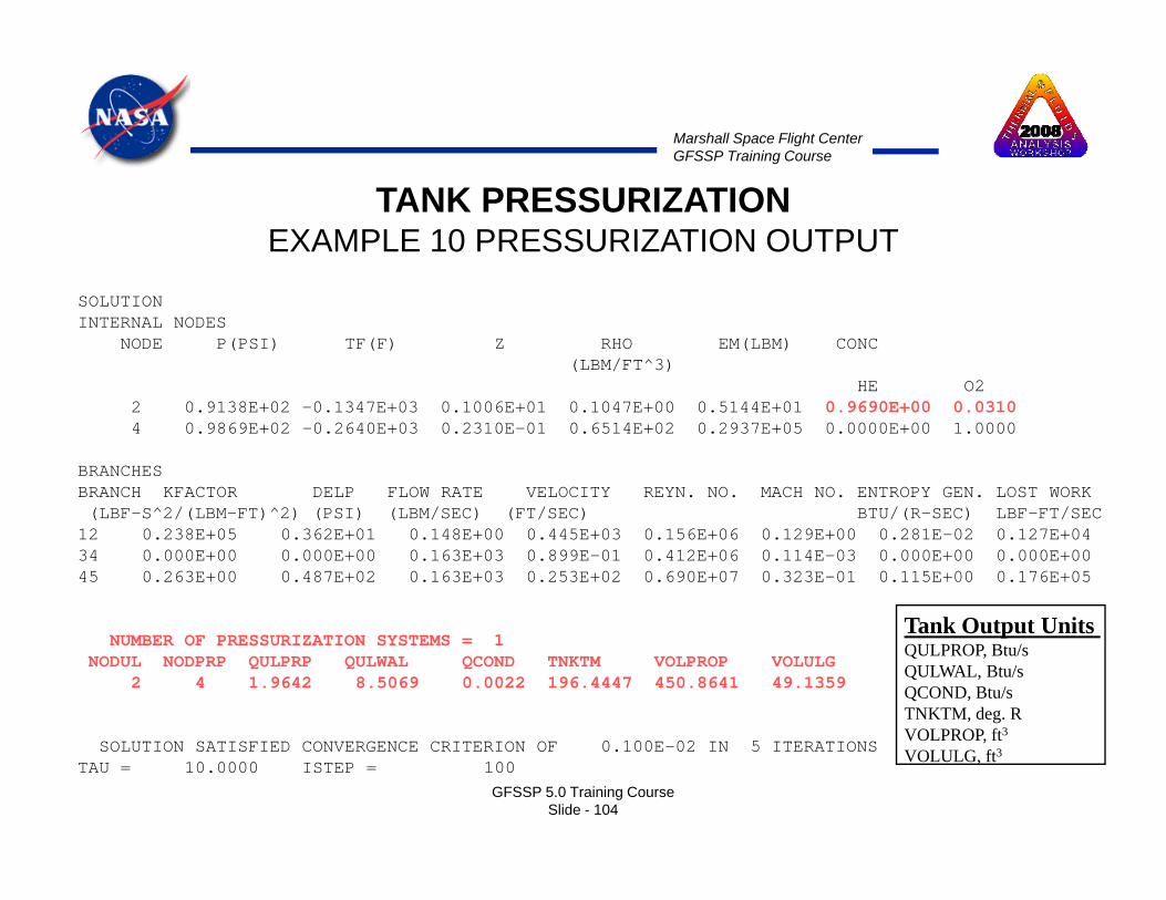
TANK PRESSURIZATIONEXAMPLE 10 PRESSURIZATION OUTPUT
SOLUTIONINTERNAL NODES
NODE P(PSI) TF(F) Z RHO EM(LBM) CONC(LBM/FT^3)
HE O2 2 0.9138E+02 -0.1347E+03 0.1006E+01 0.1047E+00 0.5144E+01 0.9690E+00 0.03104 0.9869E+02 -0.2640E+03 0.2310E-01 0.6514E+02 0.2937E+05 0.0000E+00 1.0000
BRANCHESBRANCH KFACTOR DELP FLOW RATE VELOCITY REYN. NO. MACH NO. ENTROPY GEN. LOST WORK
/ / / / /(LBF-S^2/(LBM-FT)^2) (PSI) (LBM/SEC) (FT/SEC) BTU/(R-SEC) LBF-FT/SEC12 0.238E+05 0.362E+01 0.148E+00 0.445E+03 0.156E+06 0.129E+00 0.281E-02 0.127E+0434 0.000E+00 0.000E+00 0.163E+03 0.899E-01 0.412E+06 0.114E-03 0.000E+00 0.000E+0045 0.263E+00 0.487E+02 0.163E+03 0.253E+02 0.690E+07 0.323E-01 0.115E+00 0.176E+05
T k O t t U itNUMBER OF PRESSURIZATION SYSTEMS = 1
NODUL NODPRP QULPRP QULWAL QCOND TNKTM VOLPROP VOLULG 2 4 1.9642 8.5069 0.0022 196.4447 450.8641 49.1359
Tank Output Units QULPROP, Btu/sQULWAL, Btu/sQCOND, Btu/sTNKTM, deg. RVOLPROP ft3
GFSSP 5.0 Training CourseSlide - 104
SOLUTION SATISFIED CONVERGENCE CRITERION OF 0.100E-02 IN 5 ITERATIONSTAU = 10.0000 ISTEP = 100
VOLPROP, ft3
VOLULG, ft3
Marshall Space Flight CenterGFSSP Training Course
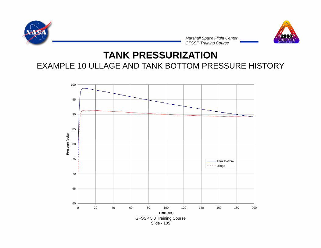
TANK PRESSURIZATIONEXAMPLE 10 ULLAGE AND TANK BOTTOM PRESSURE HISTORY
95
100
85
90
psia
)
75
80
Pres
sure
(p
Tank BottomUllage
60
65
70
GFSSP 5.0 Training CourseSlide - 105
600 20 40 60 80 100 120 140 160 180 200
Time (sec)

Marshall Space Flight CenterGFSSP Training Course
TANK PRESSURIZATIONEXAMPLE 10 ULLAGE AND TANK WALL TEMPERATURE HISTORY
-50
0
-100
50
eg F
)
-200
-150
Tem
pera
ture
(d UllageTank Wall
-250
GFSSP 5.0 Training CourseSlide - 106
-3000 20 40 60 80 100 120 140 160 180 200
Time (sec)

Marshall Space Flight CenterGFSSP Training Course
TANK PRESSURIZATIONEXAMPLE 10 HELIUM FLOW RATE HISTORY
0 35
0.4
0.45
0.25
0.3
0.35
Rat
e (lb
m/s
)
0.15
0.2
Mas
s Fl
ow R
0
0.05
0.1
GFSSP 5.0 Training CourseSlide - 107
0 20 40 60 80 100 120 140 160 180 200
Time (sec)

FLUID TRANSIENTFLUID TRANSIENT
Marshall Space Flight CenterGFSSP Training Course

Marshall Space Flight CenterGFSSP Training Course
CONTENT
• Classification of Unsteady Flow• Causes of TransientCauses of Transient• Valve Closing
C i ith M th d f Ch t i ti– Comparison with Method of Characteristics• Valve Opening• Conclusions
GFSSP 5.0 Training CourseSlide - 109

Marshall Space Flight CenterGFSSP Training Course
CLASSIFICATION OF UNSTEADY FLOW
• Quasi-steady flow is a type of unsteady flow when flow changes from one steady-state situation to another steady state situationanother steady-state situation– Time dependant terms in conservation equation is not
activated– Solution is time dependant because boundary condition is
time dependant
• Unsteady flow formulation has time dependant terms yin all conservation equations– Time dependant term is a function of density, volume and
variables at previous time step
GFSSP 5.0 Training CourseSlide - 110
variables at previous time step

Marshall Space Flight CenterGFSSP Training Course
CAUSES OF TRANSIENT
• Changes in valve settings, accidental or planned• Starting or stopping of pumps
Changes in power demand of turbines• Changes in power demand of turbines• Action of reciprocating pumps• Changing elevation of reservoirg g• Waves in reservoir• Vibration of impellers or guide vanes in pumps or
turbinesturbines• Unstable pump characteristics• Condensation
GFSSP 5.0 Training CourseSlide - 111

Marshall Space Flight CenterGFSSP Training Course
PROBLEM DESCRIPTIONRapid valve closing
D= 0 25 inch
LO2 Propellant
Tank
500 psia, -260 ° F
400 ft
D = 0.25 inch Flowrate = 0.0963 lbm/s
Time (sec) Area (in2)
0 00 0 0491
Objectives of Analysis:
Valve Closure History
0.00 0.0491
0.02 0.0164
0.04 0.0055
0.06 0.0018
• Maximum Pressure
• Frequency of Oscillation
GFSSP 5.0 Training CourseSlide - 112
0.08 0.0006
0.10 0.00

Marshall Space Flight CenterGFSSP Training Course
LO2 Propellant TankGFSSP Model
500 psia, -260 ° F
• Run a steady state model with 450 psia ambient condition
Valve
• Run unsteady model with steady state solution as initial value
• Valve closing sequence is coded in BNDUSER
Ambient
GFSSP 5.0 Training CourseSlide - 113

Marshall Space Flight CenterGFSSP Training Course
Ptank = 500 psia Ttank = -260 ° F (Oxygen) = 70 ° F (Water) = -414 ° F (Hydrogen)
Description of Test cases
Case No.
Fluid Number of Branches
Time Step (sec)
Sound Speed (ft/sec)
Flowrate (lb/sec)
pmax (psia)
Period of Oscillation
(sec) 1 LO2 10 0.01 2462 0.0963 626 0.65 2 LO2 20 0.005 2462 0.0963 632 0.65 3 LO2 5 0 02 2462 0 0966 620 0 653 LO2 5 0.02 2462 0.0966 620 0.654 H2O 10 0.005 4874 0.071 704 0.33 5 LH2 10 0.02 3577 0.0278 545 0.43 6 LO2 & GHe
(0.1%) 10 0.01 1290** 0.0963 580 1.24
7 LO2 & GHe (0.5%)
10 0.01 769** 0.0963 520 2.08
*8* LO2 (2 Phase)xexit = 0.017
10 0.01 ----- 0.0963 550 1.17
9* LO2 (2 Phase) xexit = 0.032
10 0.01 ------ 0.0963 538 1.22
10 LO2 0.01 2462 0.0963 611 0.65
* Pressure oscillations are due to condensationPressure oscillations are due to condensation** Estimated from period of oscillation [a=4L/λ]
• Time step for each test case is so chosen that Courant number is less thanunity
GFSSP 5.0 Training CourseSlide - 114
• Courant Number = Length of Branch/(Sound Speed X Time Step)

Marshall Space Flight CenterGFSSP Training Course
COMPARISON BETWEEN GFSSP &
Max. Pressure rise above
Period of Oscillation
Fluid
Flowrate (lb/s)
Velocity (ft/s)
Friction Factor
Sound Speed
COMPARISON BETWEEN GFSSP & MOC SOLUTION FOR THREE FLUIDS
supply pressure(psi)
(sec)(Used in MOC
solution)
(ft/s)
MOC GFSSP MOC GFSSP Water 0.071 3.34 0.0347 4892 214 204 0.33 0.33
Oxygen 0.0963 4.35 0.0196 2455 136 126 0.65 0.65
Hydrogen 0.0278 19.01 0.0157
3725
61
45 0.43
0.43
GFSSP 5.0 Training CourseSlide - 115

Marshall Space Flight CenterGFSSP Training Course
COMPARISON BETWEEN GFSSP & MOC SOLUTION
GFSSP 5.0 Training CourseSlide - 116

Marshall Space Flight CenterGFSSP Training Course
PROBLEM DESCRIPTIONRapid Valve Opening
D = 0 625 in
LH2 Propellant
TankInitial Pressure – 12.05 psia
200 ft
D = 0.625 inTank
112 psia, -425 ° FInitial Temperature – 60 ° F
Time (sec) Area (in2)
0.00 0.0Objectives of Analysis:0.01 0.0088
0.02 0.1767
0.03 0.2651
0.04 0.3534
• Maximum Pressure
• Time to reach steady-state
GFSSP 5.0 Training CourseSlide - 117
0.05 0.4418

Marshall Space Flight CenterGFSSP Training Course
GFSSP ModelLH2 Propellant Tank
112 psia, -425 ° F
Valve
Orifice
GFSSP 5.0 Training CourseSlide - 118

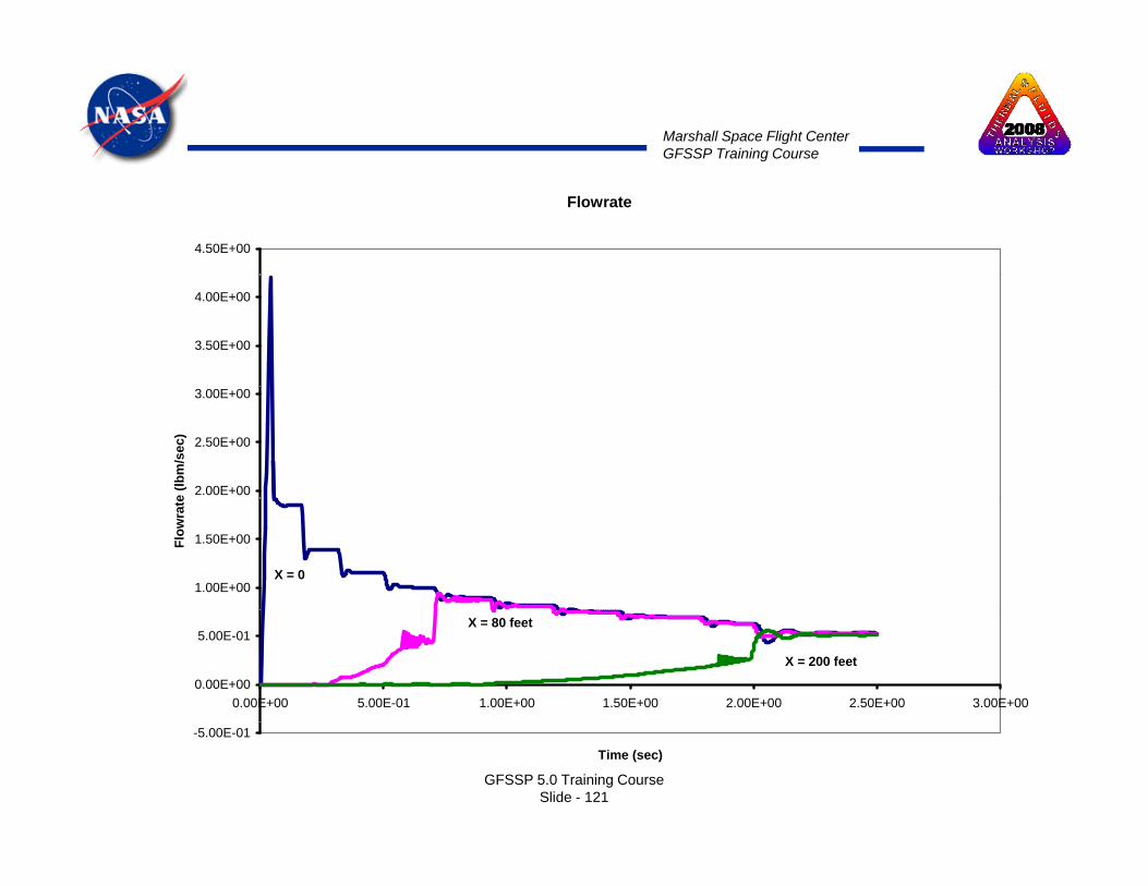
Marshall Space Flight CenterGFSSP Training Course
Pressure
3.00E+02
2.50E+02
1.50E+02
2.00E+02
P (p
sia)
1.00E+02
P
X = 0
X = 80 feet
0.00E+00
5.00E+01X = 200 feet
GFSSP 5.0 Training CourseSlide - 119
0.00E+00 5.00E-01 1.00E+00 1.50E+00 2.00E+00 2.50E+00 3.00E+00
Time (sec)

Marshall Space Flight CenterGFSSP Training Course
Temperature
6.00E+02
4.00E+02
5.00E+02
3.00E+02
T (R
)
1.00E+02
2.00E+02
X = 0 X = 80 feet X = 200 feet
0.00E+000.00E+00 5.00E-01 1.00E+00 1.50E+00 2.00E+00 2.50E+00 3.00E+00
X = 0 X = 80 feet X = 200 feet
GFSSP 5.0 Training CourseSlide - 120
-1.00E+02
Time (sec)
Marshall Space Flight CenterGFSSP Training Course
Flowrate
4.50E+00
3.50E+00
4.00E+00
2.00E+00
2.50E+00
3.00E+00
e (lb
m/s
ec)
1.00E+00
1.50E+00Flow
rate
X = 0
0.00E+00
5.00E-01
0.00E+00 5.00E-01 1.00E+00 1.50E+00 2.00E+00 2.50E+00 3.00E+00
X = 80 feet
X = 200 feet
GFSSP 5.0 Training CourseSlide - 121
-5.00E-01
Time (sec)

Marshall Space Flight CenterGFSSP Training Course
Quality
1.00E+00
7.00E-01
8.00E-01
9.00E-01
5.00E-01
6.00E-01
Qua
lity
3.00E-01
4.00E-01
0.00E+00
1.00E-01
2.00E-01
X = 0 X = 80 feet X = 200 feet
GFSSP 5.0 Training CourseSlide - 122
0.00E+00 5.00E-01 1.00E+00 1.50E+00 2.00E+00 2.50E+00 3.00E+00
Time (sec)
Marshall Space Flight CenterGFSSP Training Course
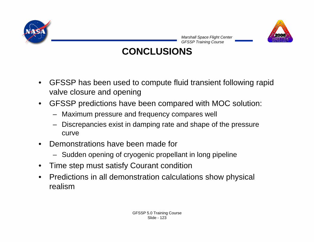
CONCLUSIONS
• GFSSP has been used to compute fluid transient following rapid valve closure and opening
• GFSSP predictions have been compared with MOC solution:GFSSP predictions have been compared with MOC solution:– Maximum pressure and frequency compares well– Discrepancies exist in damping rate and shape of the pressure
curve• Demonstrations have been made for
– Sudden opening of cryogenic propellant in long pipeline• Time step must satisfy Courant conditionTime step must satisfy Courant condition• Predictions in all demonstration calculations show physical
realism
GFSSP 5.0 Training CourseSlide - 123
C j H T fConjugate Heat Transfer
Marshall Space Flight CenterGFSSP Training Course

Marshall Space Flight CenterGFSSP Training Course
Conjugate Heat Transfer
Boundary Node Solid Node
Internal Node
Branches
Ambient Node
Conductor
Solid to Solid
Solid to Fluid
Solid to Ambient
GFSSP 5.0 Training CourseSlide - 125
Marshall Space Flight CenterGFSSP Training Course
Mathematical Closure
Unknown Variables Available Equations to Solve
1 Pressure 1 Mass Conservation Equation1. Pressure 1. Mass Conservation Equation
2. Flowrate 2. Momentum Conservation Equation
3. Fluid Temperature 3. Energy Conservation Equation of Fluid3. Fluid Temperature 3. Energy Conservation Equation of Fluid
4. Solid Temperature 4. Energy Conservation Equation of Solid
5. Specie Concentrations 5. Conservation Equations for Mass Fraction of S iSpecies
6. Mass 6. Thermodynamic Equation of State
GFSSP 5.0 Training CourseSlide - 126
Marshall Space Flight CenterGFSSP Training Course
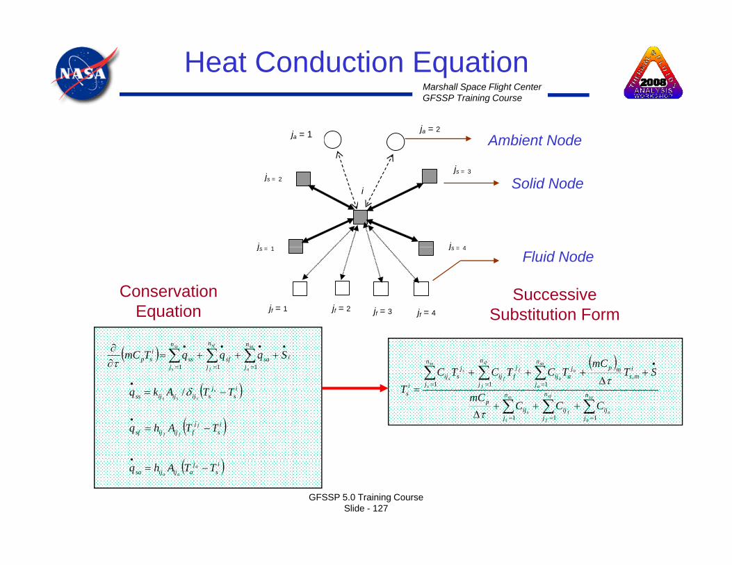
Heat Conduction Equation
jjs = 3
ja = 1 ja = 2 Ambient Node
i
j 1
js = 2
js 4
Solid Node
js = 1 js = 4
jf = 1 jf = 2 jf = 3 jf = 4
Conservation Equation
Successive Substitution Form
Fluid Node
( ) i
n
jsa
n
jsf
n
jss
isp SqqqTmC
sa
a
sf
f
ss
s
•
=
•
=
•
=
•
+++=∂∂ ∑∑∑
111
τ ( )∑ ∑ ∑
= =
•
=
+Δ
+++
=
ss
s
sf
f
sa
a
a
a
f
f
s
s
n
j
n
j
ims
mpn
j
jaij
jfij
jsij
i
STmC
TCTCTCT 1 1
,1 τ
( )ij TTAk•
δ/
q Substitution Form
∑ ∑ ∑= = =
+++Δ
=ss
s
sf
f
sa
a
afs
n
j
n
j
n
jijijij
ps
CCCmC
T
1 1 1τ
( )is
jsijijijss TTAkq s
sss−= δ/
( )is
jfijijsf TTAhq f
ff−=
•
( )•
GFSSP 5.0 Training CourseSlide - 127
( )is
jaijijsa TTAhq a
aa−=
Marshall Space Flight CenterGFSSP Training Course
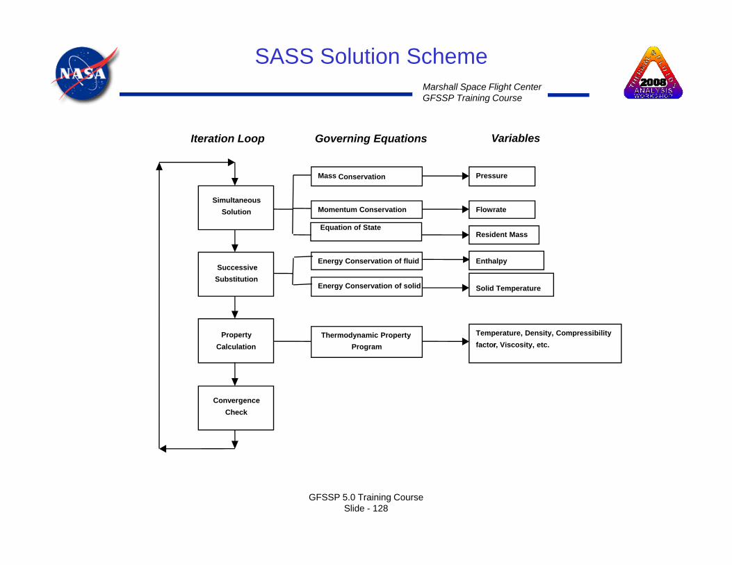
SASS Solution Scheme
Iteration Loop
Mass Conservation
Governing Equations
Pressure
Variables
Simultaneous Solution
Mass Conservation
Momentum Conservation
Equation of State
Pressure
Flowrate
Resident Mass
Successive Substitution
Energy Conservation of fluid
Energy Conservation of solid
Enthalpy
Solid Temperature
Property Calculation
Thermodynamic PropertyProgram
Temperature, Density, Compressibility factorr, Viscosity, etc.
Convergence Check
GFSSP 5.0 Training CourseSlide - 128
Marshall Space Flight CenterGFSSP Training Course
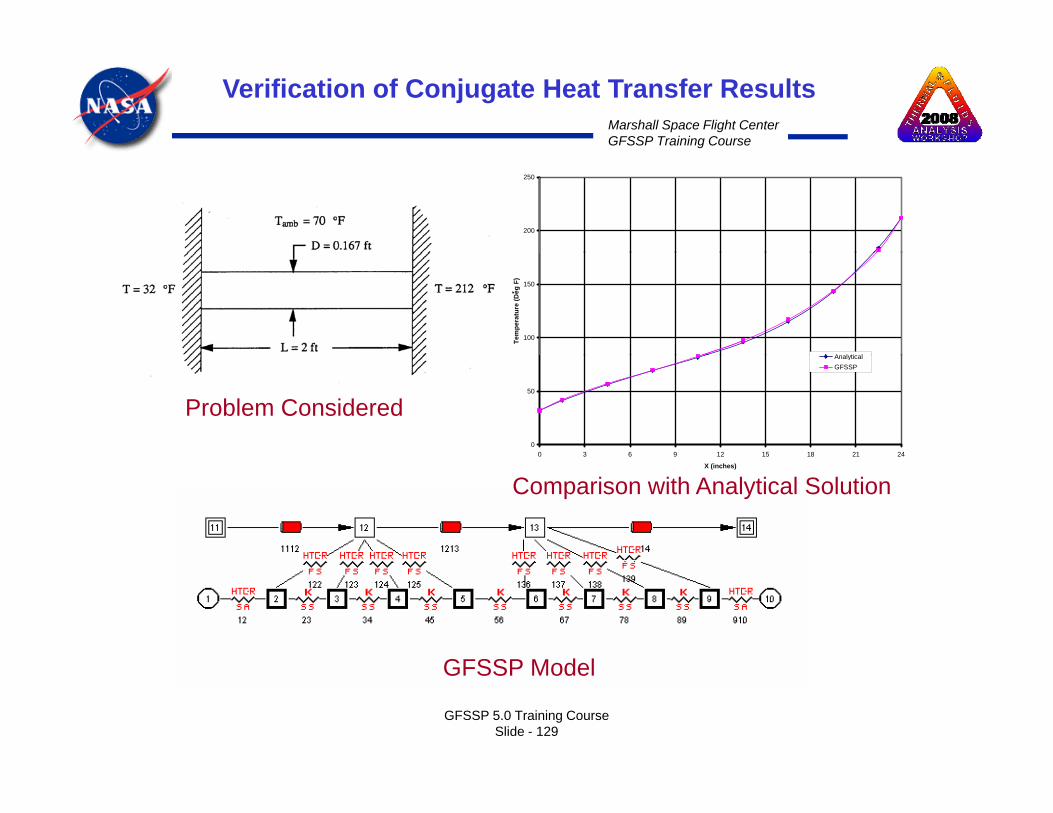
Verification of Conjugate Heat Transfer Results
200
250
100
150
Tem
pera
ture
(Deg
F)
Analytical
0
50
0 3 6 9 12 15 18 21 24
AnalyticalGFSSP
Problem Considered
X (inches)
Comparison with Analytical Solution
GFSSP Model
GFSSP 5.0 Training CourseSlide - 129
GFSSP Model

Marshall Space Flight CenterGFSSP Training Course
NBS Test Set-up of Cryogenic Transfer Line
GFSSP 5.0 Training CourseSlide - 130
Marshall Space Flight CenterGFSSP Training Course
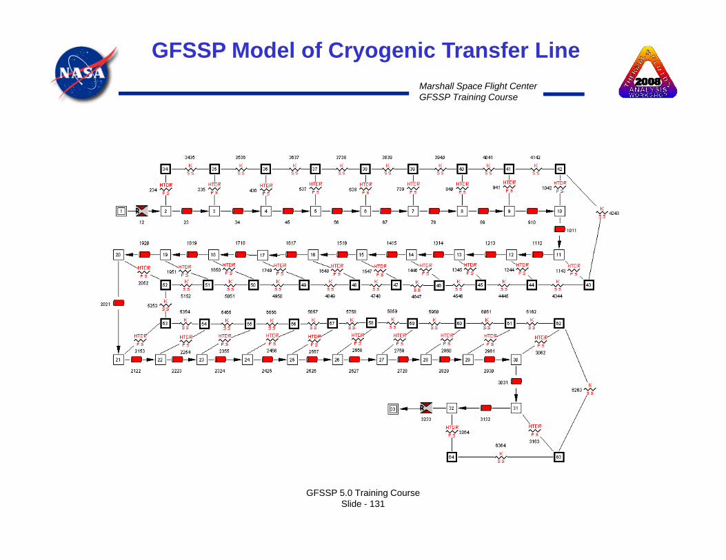
GFSSP Model of Cryogenic Transfer Line
GFSSP 5.0 Training CourseSlide - 131

Marshall Space Flight CenterGFSSP Training Course
Comparison with Test Data
300
350
Station 1 Station 2 Station 3 Station 4
250
K)
10 Node Model30 Node ModelExp Data
150
200
empe
ratu
re (K
100
Te
0
50
0 10 20 30 40 50 60 70 80 90
GFSSP 5.0 Training CourseSlide - 132
0 10 20 30 40 50 60 70 80 90Time (sec)

Marshall Space Flight CenterGFSSP Training Course
Summary
• GFSSP has been extended to model conjugate heat transfer• Fluid Solid Network Elements include:
– Fluid nodes and Flow BranchesS lid N d d A bi t N d– Solid Nodes and Ambient Nodes
– Conductors connecting Fluid-Solid, Solid-Solid and Solid-Ambient Nodes• Heat Conduction Equations are solved simultaneously with Fluid
Conservation Equations for Mass, Momentum, Energy and q gyEquation of State
• The extended code was verified by comparing with analytical solution for simple conduction-convection problem
• The code was applied to model• The code was applied to model• Pressurization of Cryogenic Tank• Freezing and Thawing of Metal• Chilldown of Cryogenic Transfer Line
GFSSP 5.0 Training CourseSlide - 133
• Boil-off from Cryogenic Tank