Getting Started with Storm Drainage Analysis using SWMM5

Robert Pitt, Alex Maestre Civil and Environmental Engineering

University of Alabama. Tuscaloosa, AL This chapter comprises the step-by-step example storm drainage design (PAT Avenue), prepared by Robert Pitt and Alex Maestre, of the Department of Civil Engineering at the University of Alabama. Introduction The US EPA National Risk Management Laboratory and CDM Inc., are rewriting the Storm Water Management Model (SWMM) software. The original version of this software was developed between 1969-1971, with Metcalf and Eddy (M&E) of Palo Alto, CA, the main contractor to develop the different modules in the program. M&E subcontracted some of the modules to Water Resources Engineers of Walnut Creek, CA (WRE) and the University of Florida (UoF). WRE (Now part of Camp Dresser and Mckee, CDM), developed the original RUNOFF, RECEIV and GRAPH models. M&E developed the RUNOFF quality and STORAGe/Treatment routines. UoF developed the TRANSPORT module. In 1973, WRE developed the TRANS model that later in 1977 was modified to EXTRAN (Larry Roesner). Also in 1977, William James developed the minicomputer version known as FASTSWMM and SWESWMM. In 1984, Computational Hydraulics Institute (CHI), the company formed by William James, developed the first user-friendly microcomputer version known as PCSWMM. In 1988, version 4 of SWMM was released by EPA and included some of the enhancements developed by PCSWMM. Since that time, the UoF (Wayne Huber and Jim Heaney), University of Guelph (where William James taught) and Oregon State University (Wayne Huber) have been improving version 4, with the release of version 4.4gu in 1999 (James 2002). SWMM5 was developed for many reasons: the previous versions were developed in DOS-based FORTRAN over more than 30 years with different levels of documentation. The development of the Windows environment and object oriented programming techniques improved programming capabilities and graphical user interfaces. One advantage of the new model is that only a single file is needed, and not multiple modules, for a single simulation. A single file can now be created that contains RUNOFF, TRANSPORT and/or EXTRANS at the same time. SWMM5 uses the same environment that EPANET uses, assigning the values to the objects used during the simulation. Other reasons for the new SWMM version are its ability to eventually develop routines for modeling Best Management Practices (BMP’s) for runoff control, to improve the routing procedures of water quality in the model, and to create the possibility to simulate Real Time Control by manipulating control structures (EPA 2002).

1

STARTING SWMM5 The model can be downloaded by going to the EPA web site: http://www.epa.gov/ednnrmrl/swmm/beta_test.htm Copy the program to your computer and follow the installation instructions. To start the program, go to the shortcut located on your desktop, or select start/programs/SWMM5.

Figure 1

CREATING A NEW PROJECT To start the program, go to the shortcut located on your desktop, or select start/programs/SWMM5. The SWMM 5 environment consist of seven areas: Main Menu, Main Toolbar, Drawing Element Toolbar, Data and Map Browser, SWMM controls, Properties, and the Drawing Area.

2

Figure 2. SWMM5 Environment

“Hello World” Pat Avenue Storm Drainage Design Example This is a very simple example intended to show the user how to access the main components of SWMM5 and to create and run a simple model. After going through this example, it should be much easier to follow more complex examples, or to enter site-specific information for a larger site. Pat Avenue is located in Birmingham, AL. It consists of three subcatchments, three junctions (nodes) and two conduits (pipes) in a residential area. The water collected during a rainstorm is discharged to a main sewer trunk. Figure 3 shows the watershed delineation for Pat Avenue.

Figure 3. PAT Avenue subcatchments, joints and conduits.

3

The description of each subcatchment is shown in Table 1. Table 1. Pat Avenue Subcatchment information: SUBCATCHMENT Area

(Acres) Width

(ft) Slope (ft/ft)

Percentage of imperviousness

n Manning impervious

n Manning pervious

1001 1.067 98.3 0.084 54 0.040 0.410 1011 1.087 74.5 0.093 54 0.040 0.410 1021 1.431 109.0 0.072 54 0.040 0.410

SUBCATCHMENT Horton maximum

infiltration rate (in/hr) Horton minimum

infiltration rate (in/hr) Horton decay coefficient

(1/sec) 1001 1 0.1 0.002 1011 1 0.1 0.002 1021 1 0.1 0.002

The three subcatchments are similar in all the parameters except area, slope and width. The width of the watershed can be calculated as the ratio of the area to the longest flow path in the watershed. This is a critical attribute that affects the watershed time of concentration. The infiltration parameters are the same for all three subcatchments. The junction properties are shown in Table 2: Table2. Pat Avenue Junction Information:

JUNCTION Invert

Elevation (ft)

Maximum Depth (ft)

Initial Depth (ft)

Surcharge Depth (ft)

Ponded Area (ft²)

100 791 10 0 0 0 101 769 10 0 0 0 102 753 10 0 0 0

The invert elevation corresponds to the elevation of the corresponding junction. The maximum depth is the distance from the bottom of the junction to the ground surface. The surcharge depth is the additional water depth above the ground surface used to store water during surcharge conditions. The ponded area is the surface area of the water accumulated during the surcharge. The conduit information is shown in Table 3. Table 3. Pat Avenue Conduit Information: CONDUIT Shape Diameter

(ft) Length

(ft) n Manning Inlet invert height (ft)

1000 Circular 1 300 0.013 0.5 1001 Circular 1 300 0.013 0.5

CONDUIT Outlet invert

height (ft) Initial

flow (cfs) Entry loss coefficient

Exit loss coefficient

Average loss coefficient

1000 0.5 0 0 0 0 1001 0.5 0 0 0 0

There are two circular concrete pipes, each 1 ft in diameter. The length of each pipe is 300 ft. There is no initial flow in the pipe and entrance and exit losses are negligible. There is no flap gate at the end on the pipe.

4

Figure 4. PAT Avenue’s joints and conduits characteristics.

CREATING A NEW PROJECT The first step is to name the project. Click on the data browser tab and select the Title/Notes option. In the properties area, a green plus sign will appear. Click on the green plus to add a title to the project. After assigning the title, you will be able to use the remaining options. The red minus sign will delete the object, and the yellow finger will edit the object. The remaining options will move up, move down or order the elements in the properties box. Return to the data browser and double click on the options category. The edit option will be active in the properties area. In order to display the properties, it is possible to click the edit button, or double click on the desired option. Press the edit button to display the properties of the project. In the general tab, select the desired units. In this case the units are in US. customary system. Select flow units in cubic feet per second (cfs). The infiltration model used is Horton, but the Green Ampt and NRCS Curve Number procedures are also available. The routing model used during this example is the kinematic wave as a continuity equation for lateral flow in an unsteady channel. In the dynamic wave option (important for unsteady flow used evaluating CSOs and SSOs in sanitary sewage systems, for example) all the Saint Venant equations are used. Chow (1988) presents a description of the two models in the distributed flow routing chapter.

801 ft779 ft

300 ft

300 ft

763 ft

10 ft

10 ftD = 1ft n = 0.013

D = 1ft n = 0.013

5

Continuity Equations:

Conservation Form 0=∂∂

+∂∂

tA

xQ

Nonconservation Form 0=∂∂

+∂∂

+∂∂

ty

xVy

xyV

Momentum Equations:

Conservation Form 0)(11 2

=−−∂∂

+⎟⎟⎠

⎞⎜⎜⎝

⎛∂∂

+∂∂

fo SSgxyg

AQ

xAtQ

A

0)( =−− fo SSg Kinematic Wave

0)( =−−∂∂

fo SSgxyg Diffusion Wave Nonconservation

Form 0)( =−−

∂∂

+∂∂

+∂∂

fo SSgxyg

xVV

tV

Dynamic Wave

In this case, no ponding is allowed at the manholes. Uncheck this option in the general tab. Select now the dates tab on the same window. Assume this simulation started on January 1, 2003 at 00:00 and had a 24 hour duration, in Birmingham Alabama. The analysis will end on January 2, 2003. The number of antecedent dry days is zero (it rained immediately before this simulated event). Click on the Time Steps tab. Select the time steps according to the rain file. In this example, the rain file has data every 30 minutes. There is no dry weather precesses simulated, and the default 1 hour time step can be selected. Select a 5-minute routing time step and a 30-minute reporting time step. The dynamic wave and Interface files tabs are not used in this example. Now you will import a time series with the precipitation for a 24-hour type II event, corresponding to Birmingham, AL. In the data browser, select the Time Series option and in the properties area add a new series. In the name field, assign the name “TypeII” without quotes. Now press the load button and select the file TypeII.dat. Click the view button to observe the 24-hour hydrograph. Close the window and click OK to accept the time series. Figure 5 shows the 24-hour type II rain.

6

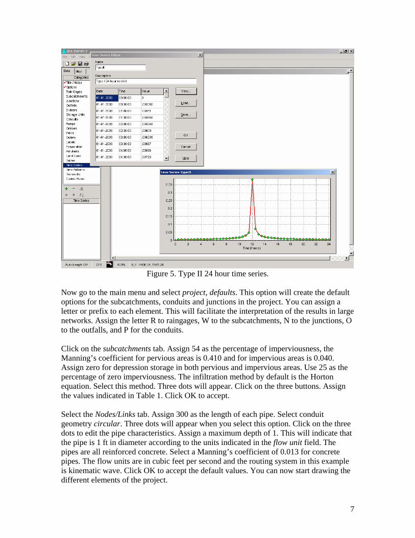
Figure 5. Type II 24 hour time series.

Now go to the main menu and select project, defaults. This option will create the default options for the subcatchments, conduits and junctions in the project. You can assign a letter or prefix to each element. This will facilitate the interpretation of the results in large networks. Assign the letter R to raingages, W to the subcatchments, N to the junctions, O to the outfalls, and P for the conduits. Click on the subcatchments tab. Assign 54 as the percentage of imperviousness, the Manning’s coefficient for pervious areas is 0.410 and for impervious areas is 0.040. Assign zero for depression storage in both pervious and impervious areas. Use 25 as the percentage of zero imperviousness. The infiltration method by default is the Horton equation. Select this method. Three dots will appear. Click on the three buttons. Assign the values indicated in Table 1. Click OK to accept. Select the Nodes/Links tab. Assign 300 as the length of each pipe. Select conduit geometry circular. Three dots will appear when you select this option. Click on the three dots to edit the pipe characteristics. Assign a maximum depth of 1. This will indicate that the pipe is 1 ft in diameter according to the units indicated in the flow unit field. The pipes are all reinforced concrete. Select a Manning’s coefficient of 0.013 for concrete pipes. The flow units are in cubic feet per second and the routing system in this example is kinematic wave. Click OK to accept the default values. You can now start drawing the different elements of the project.

7

The second button in the SWMM elements is the subcatchment element. Click on it to start drawing the first watershed. A pencil will appear in the drawing area. Click the left mouse button and trace the watershed 1001 similar to that presented in Figure 3. Use the right mouse button to close the watershed drawing. Once you finish, you will have a drawing similar to the subcatchment shown in Figure 6.

Figure 6. Subcatchment 1001

In the main toolbar, use the selector, the black arrow to select elements. It is the seventh button from right to left in the main toolbar. Now click on the blinking square inside the watershed. Assign the description and tag fields “W1001”, without the quotes. Complete the area, width and slope information for this watershed. Check that the infiltration information is correct and close the window. Select the junction button located below the subcatchment button. Locate the junction in the far East corner of the subcatchment 1001, outside the subcatchment. Use the selector to display the properties of the junction. Double click on the junction to display the properties. Assign N100 in the description and tag fields. There is no external or dry weather flow in this junction. The invert elevation of this junction is located 10 ft below the ground surface. Use 791 to assign the elevation of the junction and 10 as the maximum depth. Initial depth, surcharge depth and ponded area are zero in this case. Close the window.

8

Double click again in the square located inside the subcatchment. Assign “N1” without quotes to the field outlet. This will indicate that the water produced in this subcatchment will reach the first junction. Close the window. A dotted line will appear between the square and the junction. Now a raingage will be created. Click on the button located above the watershed button. It is similar to a cloud raining. Locate the raingage as shown in Figure 7.

Figure 7. Raingage location.

Use the selector from the main toolbar. Double click on the raingage to display its properties. Assign “Raingage 1” without quotes to the description and tag fields. Click now on the series name. A drop-down menu will appear, select “Type II”. Close the window. Return to the subcatchment and edit the properties. Click on the raingage field. A drop down menu will appear, select R1 as the raingage 1 selected. Close the window. (Have you saved the project recently?) Now you have everything connected and can continue with the second subcatchment. Because this program is object oriented it is recommended that you draw each element separately. Draw the second subcatchment a little displaced to the right without touching the previous watershed or the junction 100. Figure 8 shows the drawing area after drawing the second watershed. Complete the information using the information in

9

Table1. Use the raingage 1 also for this watershed. You can not assign the outlet information at this moment.

Figure 8. Raingage location.

Select the junction button and draw the junction 101. This junction is located at 769 ft and has a maximum depth of 10 ft. Close the window. Return to the subcatchment 1011 and update the outlet information. Assign to the outlet field “N2” without the quotes. To create the conduit between the junctions 100 and 101, select the seventh button in the SWMM elements toolbar. Click on the junction 100 and in the junction 101 to create the pipe. Use the selector. Double click on the conduit to display the properties. You can also click on the little yellow hand located on the properties window. Assign “P1000” without the quotes to the description and tag field. Use Table 3 to complete the information of the conduit. Now create the last watershed using the watershed button and use the information from Table 1 to complete the required data. The last Junction will be modeled as an outfall. Select the fourth element on the SWMM elements toolbar. The outfall element is located below the junction element. Display its properties. Assign “N102” without quotes in the description and tag fields. Assign an invert elevation of 753 ft. There is no tide gate. It is modeled as a free discharge. The last element is the pipe1001, create this element and update the information using Tables 1, 2 and 3. The final sketch of the system is shown in Figure 9.

10

Figure 9. Final Sketch

The rain file used with the raingage is the standard file for one inch precipitation. Assume in this example that the total rainfall during the 24 hours is 6.4 in. You can multiply the original file using the option Time Patterns in the data browser. Select Time Patterns, now add a new pattern in the properties window. Select type, daily. Assign the name “Design” without quotes, and describe it as a design event for 6.4 in. precipitation. The details of the final SWMM5 file can be observed under project/details in the main menu. The following is the final entry file after adding all the data. [TITLE] Pat Avenue - SWMM5 Alex Maestre [OPTIONS] FLOW_UNITS CFS INFILTRATION HORTON FLOW_ROUTING KW START_DATE 01-01-2003 START_TIME 00:00 REPORT_START_DATE 01-01-2003 REPORT_START_TIME 00:00 END_DATE 01-02-2003 END_TIME 00:00 DRY_DAYS 0 WET_STEP 00:15:00 DRY_STEP 01:00:00 ROUTING_STEP 00:05:00 REPORT_STEP 00:15:00 INERTIAL_DAMPING 1

11

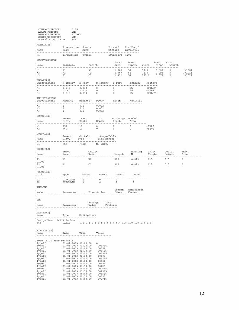
COURANT_FACTOR 0.75 ALLOW_PONDING YES DYNWAVE_METHOD PICARD SLOPE_WEIGHTING YES NORMAL_FLOW_LIMITED YES [RAINGAGES] ; Timeseries/ Source Format/ RecdFreq/ ;Name File Name Station RecdIntvl ;------------------------------------------------------------------- R1 TIMESERIES TypeII INTENSITY 1:00 [SUBCATCHMENTS] ; Total Pcnt. Pcnt. Curb ;Name Raingage Outlet Area Imperv Width Slope Length ;--------------------------------------------------------------------------------------------- W1 R1 N1 1.067 54 98.7 0.084 0 ;W1001 W2 R1 N2 1.087 54 74.5 0.093 0 ;W1011 W3 R1 O1 1.431 54 109.0 0.072 0 ;W1021 [SUBAREAS] ;Subcatchment N-Imperv N-Perv S-Imperv S-Perv pctZERO RouteTo ;------------------------------------------------------------------------------- W1 0.040 0.410 0 0 25 OUTLET W2 0.040 0.410 0 0 25 OUTLET W3 0.040 0.410 0 0 25 OUTLET [INFILTRATION] ;Subcatchment MaxRate MinRate Decay Regen MaxInfil ;--------------------------------------------------------------------- W1 1 0.1 0.002 W2 1 0.1 0.002 W3 1 0.1 0.002 [JUNCTIONS] ; Invert Max. Init. Surcharge Ponded ;Name Elev. Depth Depth Depth Area ;------------------------------------------------------------------------ N1 791 10 0 0 0 ;N100 N2 769 10 0 0 0 ;N101 [OUTFALLS] ; Invert Outfall Stage/Table ;Name Elev. Type Time Series ;---------------------------------------------------- O1 753 FREE NO ;N102 [CONDUITS] ; Inlet Outlet Manning Inlet Outlet Init. ;Name Node Node Length N Height Height Flow ;------------------------------------------------------------------------------------------------------------ P1 N1 N2 300 0.013 0.5 0.5 0 ;P1000 P2 N2 O1 300 0.013 0.5 0.5 0 ;P1001 [XSECTIONS] ;Link Type Geom1 Geom2 Geom3 Geom4 ;------------------------------------------------------------------------- P1 CIRCULAR 1 0 0 0 P2 CIRCULAR 1 0 0 0 [INFLOWS] ; Concen Conversion ;Node Parameter Time Series /Mass Factor ;---------------------------------------------------------------------- [DWF] ; Average Time ;Node Parameter Value Patterns ;----------------------------------------------------- [PATTERNS] ;Name Type Multipliers ;--------------------------------------- ;Design Event P=6.4 inches p64 DAILY 6.4 6.4 6.4 6.4 6.4 6.4 6.4 1.0 1.0 1.0 1.0 1.0 [TIMESERIES] ;Name Date Time Value ;------------------------------------------------- ;Type II 24 hour rainfall TypeII 01-01-2003 00:00:00 0 TypeII 01-01-2003 00:30:00 .005365 TypeII 01-01-2003 01:00:00 .00551 TypeII 01-01-2003 01:30:00 .005655 TypeII 01-01-2003 02:00:00 .005945 TypeII 01-01-2003 02:30:00 .00609 TypeII 01-01-2003 03:00:00 .006235 TypeII 01-01-2003 03:30:00 .00667 TypeII 01-01-2003 04:00:00 .00696 TypeII 01-01-2003 04:30:00 .00725 TypeII 01-01-2003 05:00:00 .007685 TypeII 01-01-2003 05:30:00 .007975 TypeII 01-01-2003 06:00:00 .008555 TypeII 01-01-2003 06:30:00 .00899 TypeII 01-01-2003 07:00:00 .009715

12

TypeII 01-01-2003 07:30:00 .01044 TypeII 01-01-2003 08:00:00 .011455 TypeII 01-01-2003 08:30:00 .01247 TypeII 01-01-2003 09:00:00 .01392 TypeII 01-01-2003 09:30:00 .015805 TypeII 01-01-2003 10:00:00 .01827 TypeII 01-01-2003 10:30:00 .023345 TypeII 01-01-2003 11:00:00 .030885 TypeII 01-01-2003 11:30:00 .048285 TypeII 01-01-2003 12:00:00 .38019 TypeII 01-01-2003 12:30:00 .07192 TypeII 01-01-2003 13:00:00 .037265 TypeII 01-01-2003 13:30:00 .026535 TypeII 01-01-2003 14:00:00 .02088 TypeII 01-01-2003 14:30:00 .01827 TypeII 01-01-2003 15:00:00 .015805 TypeII 01-01-2003 15:30:00 .013775 TypeII 01-01-2003 16:00:00 .01247 TypeII 01-01-2003 16:30:00 .01131 TypeII 01-01-2003 17:00:00 .01044 TypeII 01-01-2003 17:30:00 .00957 TypeII 01-01-2003 18:00:00 .009135 TypeII 01-01-2003 18:30:00 .008555 TypeII 01-01-2003 19:00:00 .007975 TypeII 01-01-2003 19:30:00 .00754 TypeII 01-01-2003 20:00:00 .00725 TypeII 01-01-2003 20:30:00 .00696 TypeII 01-01-2003 21:00:00 .006525 TypeII 01-01-2003 21:30:00 .00638 TypeII 01-01-2003 22:00:00 .005945 TypeII 01-01-2003 22:30:00 .005945 TypeII 01-01-2003 23:00:00 .005655 TypeII 01-01-2003 23:30:00 .00551 TypeII 01-02-2003 00:00:00 .005365

Now you can run the model. In the main toolbar, click the seventh button from the left. The symbol is a green triangle like a play button. If the run was successful, a window will be displayed showing the successful run label. Figure 10 shows a successful run.

Figure 10. Final Sketch

13

It is possible to observe the results under report/status in the main menu. An example of the results is as follows. EPA STORM WATER MANAGEMENT MODEL - VERSION 5.0B (Build 7/28/03) ----------------------------------------------- Pat Avenue - SWMM5 Alex Maestre **************** Analysis Options **************** Flow Units ................ CFS Infiltration Method ....... HORTON Flow Routing Method ....... KW Starting Date ............. JAN-01-2003 00:00:00 Ending Date ............... JAN-02-2003 00:00:00 Wet Time Step ............. 00:15:00 Dry Time Step ............. 01:00:00 Routing Time Step ......... 00:05:00 Report Time Step .......... 00:15:00 ***************** Volume Depth Runoff Continuity acre-feet inches ***************** --------- ------- Total Precipitation ..... 0.148 0.495 Total Losses ............ 0.000 0.000 Total Runoff ............ 0.120 0.401 Initial Storage ......... 0.000 0.000 Final Storage ........... 0.028 0.095 Continuity Error (%) .... -0.165 ************************* Volume Flow Transport Continuity cubic ft ************************* --------- Dry Weather Inflow ...... 0.000e+00 Wet Weather Inflow ...... 5.213e+03 External Inflow ......... 0.000e+00 External Outflow ........ 5.211e+03 Initial Stored Volume ... 6.000e-02 Final Stored Volume ..... 4.433e+00 Continuity Error (%) .... -0.041 ****************** Node Depth Summary ****************** ---------------------------------------------------------------------------------------- Average Maximum Time of Max Average Total Fraction Depth Depth Occurrence Depth Minutes Courant Node Feet Feet days hr:min Change Flooded Critical ---------------------------------------------------------------------------------------- JUNCTION N1 0.53 0.58 0 13:00 0.0023 0 0.00 JUNCTION N2 0.54 0.62 0 13:05 0.0025 0 0.00 OUTFALL O1 0.00 0.00 0 00:00 0.0000 0 0.00 ******************** Conduit Flow Summary ******************** --------------------------------------------------------------------------------------- Maximum Time of Max Maximum Time of Max Maximum Total Flow Occurrence Velocity Occurrence /Design Minutes Conduit CFS days hr:min ft/sec days hr:min Flow Surcharged --------------------------------------------------------------------------------------- P1 1.33e-01 0 13:00 4.34 0 13:00 0.01 0 P2 2.48e-01 0 13:05 4.72 0 13:05 0.03 0 Analysis begun: Fri Oct 31 11:05:28 2003 Analysis ended: Fri Oct 31 11:05:28 2003

OBSERVING THE RESULTS Select the map browser. Select runoff in the subcatchment view menu, depth in the node view menu, and flow in the link menu. In the elapsed time field, there are two arrows. Press the up arrow to observe the change in flow in the watershed and pipes. You can also observe the results in the automatic mode. Go to view in the main menu, select toolbars/animator. The lower button in the animator increases or decreases the

14

speed of the simulation. The left arrow rewinds the simulation and the right button plays it. The results can be observed also in a table. Go to Report/table/by variable in the main menu. Select as object category: links and as variable: flow. On the map, click conduit 1000, now click the plus sign in the table by variable window. Now click on the conduit 1001 and click the plus sign to add it to the table. Click OK and the results will be displayed in a table.

Figure 11. Graphical Results

The third option is to show the results in a profile. In the main menu, select Report/graph/profile. On the map, click junction 100, now return to the window and click the plus sign next in the start node field. Now click node 102on the map. Click the plus sign in the end node field. Click on find the path and click OK to display the profile. You can use the animator option to observe how the profile changes during the simulation. Figure 12 shows a profile for PAT Avenue.

15

Figure 12. Profile

REFERENCES http://www.epa.gov/ednnrmrl/swmm/beta_test.htm US EPA, National Risk Management Research Laboratory, Office of Research and

Development, (2002). SWMM Redevelopment Project Plan. Version 5. Water Supply and Water Resources Division.

James, W., W. Huber, R. Pitt, R. Dickinson, and R. James (2002). Water Systems Models, Hydrology. CHI, Guelph Ontario Canada. 347 pp.

Chow V., (1988). Applied Hydrology. McGraw Hill Book Co. – New York.

16