Clemson UniversityTigerPrints

All Theses Theses

8-2014

GETTING SANDY: CREATING COLLAPSINGSAND EFFECTS FOR AN ODE TO LOVEPisut WisessingClemson University, pwisess@clemson.edu

Follow this and additional works at: https://tigerprints.clemson.edu/all_theses

Part of the Computer Sciences Commons, Film and Media Studies Commons, and the Fine ArtsCommons

This Thesis is brought to you for free and open access by the Theses at TigerPrints. It has been accepted for inclusion in All Theses by an authorizedadministrator of TigerPrints. For more information, please contact kokeefe@clemson.edu.

Recommended CitationWisessing, Pisut, "GETTING SANDY: CREATING COLLAPSING SAND EFFECTS FOR AN ODE TO LOVE" (2014). All Theses.1898.https://tigerprints.clemson.edu/all_theses/1898

GETTING SANDY: CREATING COLLAPSING SAND EFFECTS FOR AN ODE TO LOVE

_________________________________________

A Thesis Presented to

The Graduate School of Clemson University

_________________________________________

In Partial Fulfillment of the Requirements for the Degree

Master of Fine Arts Digital Production Arts

_________________________________________

by Pisut Wisessing

August 2014 _________________________________________

Accepted by:

Dr. Timothy Davis, Committee Chair Dr. Donald House Prof. Tony Penna

ii

ABSTRACT

This thesis presents an artistic approach of creating collapsing sand effects in

Brown Bag Films’ animated short, An Ode To Love, directed by Matthew Darragh. A

combination of rigid body simulation and fluid simulation tools, which are available in

Houdini 3D animation software version 13, was used to successfully complete the task. A

detailed design and implementation process to achieve the effects is documented in this

work.

iii

TABLE OF CONTENTS

Page

TITLE PAGE ................................................................................................................ i

ABSTRACT .................................................................................................................. ii

LIST OF FIGURES ...................................................................................................... v

CHAPTER ONE: INTRODUCTION ............................................................................ 1

CHAPTER TWO: BACKGROUND ............................................................................. 5

2.1 Particle-Based Simulation of Granular Materials .................................................... 5

2.2 Animated Sand as a Fluid ........................................................................................ 6

2.3 Fluid Simulation in Computer Graphics ................................................................. 7

2.4 Rigid-Body Simulation in Computer Graphics ....................................................... 10

2.5 Destruction Pipeline ................................................................................................ 11

CHAPTER THREE: IMPLEMENTATION ................................................................. 15

3.1 Workflow ................................................................................................................. 16

3.2 Fractures Preparation .............................................................................................. 17

3.3 Rigid-Body Simulation ........................................................................................... 22

3.4 Fluid Preparation ..................................................................................................... 26

3.5 Fluid Simulation ..................................................................................................... 28

3.6 Rendering ................................................................................................................. 30

3.7 Extra Sand Particles ................................................................................................ 33

CHAPTER FOUR: RESULTS ...................................................................................... 34

iv

TABLE OF CONTENTS (CONTINUED)

Page

CHAPTER FIVE: DISCUSSION AND FUTURE WORK ......................................... 40

5.1 Easier Controls ........................................................................................................ 40

5.2 Better Performance ................................................................................................. 40

5.3 More Generalized Sand Solver ............................................................................... 41

REFERENCES .............................................................................................................. 43

v

LIST OF FIGURES

Page

Figure 1.1: The short film, An Ode To Love ............................................................... 1

Figure 1.2: Sandman’s collapsing hand ...................................................................... 3

Figure 1.3: Video reference of the collapsing sand effects in An Ode To Love .......... 4

Figure 2.1: Result from Particle-Based Simulation of Granular Materials

by Bell et al. [BYM05] ............................................................................... 6

Figure 2.2: Result from Animating Sand as a Fluid by Zhu et al. [ZB05] .................... 7

Figure 2.3: Comparison of particle and grid representations of a fluid ...................... 9

Figure 2.4: Los Angeles destruction in 2012 created with Bullet Physics Engine ..... 11

Figure 2.5: Voronoi diagram with feature points ....................................................... 12

Figure 2.6: A concave geometry fractured with Voronoi sub division ....................... 13

Figure 2.7: Example of multiple-level constraint networks ....................................... 14

Figure 3.1: Art keys of the collapsing sand effects by Rianti Hidayat ........................ 15

Figure 3.2: Workflow for creating collapsing sand effects ......................................... 16

Figure 3.3: Voronoi fracture node in Houdini ............................................................ 17

Figure 3.4: Uninteresting fractures with straight edges ............................................... 18

Figure 3.5: Reference showing a sand mound falling apart ........................................ 18

Figure 3.6: Sand mound broken into outer piece and inner piece ............................... 19

Figure 3.7: Child pieces grouped together based on proximity to parents ................. 20

Figure 3.8: Houdini network for the fractures preparation stage ............................... 21

Figure 3.9: Rigid-body objects activation control network ........................................ 22

vi

LIST OF FIGURES (CONTINUED)

Page

Figure 3.10: Activation order and simulation result ..................................................... 23

Figure 3.11: Relaxing collision condition inside rigid-body simulation network ........ 25

Figure 3.12: Inactive objects remaining as chunks, and active fluid objects turning

Into particles ............................................................................................. 28

Figure 3.13: Houdini network of fluid preparation stage ............................................. 28

Figure 3.14: Houdini network for FLIP simulation with reseeding unchecked ........... 29

Figure 3.15: Inactive and active fluid objects used as collision volumes in FLIP ....... 30

Figure 3.16: Keeping fracturing and scattering particles consistent and avoiding

pops with a lattice deformer .................................................................... 31

Figure 3.17: Randomizing color and size of the particles ............................................ 32

Figure 3.18: Sand mound with randomized color and size .......................................... 32

Figure 3.19: Extra sand particles added on top ............................................................. 33

Figure 4.1: Result from rigid-body simulation ........................................................... 35

Figure 4.2: Result from fluid simulation .................................................................... 36

Figure 4.3: Combined result from rigid-body simulation and fluid simulation ......... 37

Figure 4.4a: Final image from An Ode To Love ............................................................ 38

Figure 4.4b: Final image from An Ode To Love ............................................................ 39

Figure 5.1: Result from A Material Point Method for Snow Simulation [SSC+13] .. 42

1

CHAPTER ONE

INTRODUCTION

Figure 1.1: The short film, An Ode To Love © Brown Bag Films

A small team of artists at Brown Bag Films, led by Matthew Darragh, recently

produced an animated short, An Ode To Love (Figure 1.1). Since the story is set on

a remote sandy island, numerous shots involved the character interacting closely with

sand. Many technical challenges arose during the production process, with the collapsing

sand mound scene one of the most difficult. Because of limited production time and

computing resources available, as well as specific art direction, a fast and effective

technique was required to handle the sand effects. After examining works related to sand

animation in computer graphics, an artistic approach, referred to as “hacks,” was

developed to complete the collapsing sand effects needed for the film.

2

Creating a natural phenomenon such as sand dynamics requires research and

development for computer graphics due to its complex material properties. Sand can

behave like particles, with each individual grain moving independently in microscale

when observed closely. From a distance, the aggregate of thousands or even millions of

sand particles seem to behave as either a viscous fluid or a shape-shifting deformable

object. It can flow from higher ground to lower ground under the influence of gravity, or

can smoothly deform when stepped upon.

Many attempts have been made to recreate the dynamics of sand in the virtual

world of computer graphics. In academia, Bell et al. used simplified particle- and rigid-

body systems to imitate a small amount of sand movement [BYM05]. The technique was

accurate; however, it could not be scaled adequately for large scenes due to the heavy

computational requirements. Zhu et al., on the other hand, took a different approach,

extending a fluid solver to simulate sand in large-scale environments [ZB05] . The

outcome was impressive with relatively accurate results for large amounts of sand.

In visual effects and computer animation productions, one of the early notable

sand simulations appears in Spider-Man 3, created by a team at Sony Pictures

Imageworks [ABC+07]. They applied the “tricks” of particles and rigid-body simulation

available at the time to create the Sandman, in both human-sized form (Figure 1.2) and a

60-foot-tall version.

3

Figure 1.2: Sandman’s collapsing hand © Columbia Pictures

For the collapsing sand shot in An Ode To Love, a video reference was used that

depicted a sand castle breaking into chunks before turning into small sand particles

(Figure 1.3). No off-the-shelf tool could produce the work according to the director’s

vision right out of the box. Further, the time and resources for research to develop a

generalized standalone sand simulation system was not worth the effort since the

collapsing sand would appear in only one shot. As a result, the inspiration from the

aforementioned works, Zhu’s fluid approach in particular, was utilized in Houdini

software to complete the effects. Ultimately, a mix of rigid-body simulation and fluid

simulation tools were used to achieve the desired look and feel.

4

Figure 1.3: Video reference of the collapsing sand effects in An Ode To Love [San14a]

5

CHAPTER TWO

BACKGROUND

Past notable works in sand animation, such as Particle-Based Simulation of

Granular Materials by Bell et al. [BYM05], and Animating Sand as a Fluid by Zhu et al.

[ZB05], are good starting points for our collapsing sand effects. Next, the basic

understanding of fluid simulation and state-of-the-art Fluid-Implicit-Particle (FLIP)

method will be covered with the goal of modifying existing Houdini FLIP simulation

tools for the desired sand behavior. Finally, the popular Bullet Physics Engine and a

destruction pipeline for visual effects will be briefly introduced. These two techniques are

effective in creating art-direct able destruction sequences.

2.1 Particle-Based Simulation of Granular Materials

Bell et al. approached the sand and general granular material simulation with

discrete representations [BYM05]. Individual sand particles were modeled as small

sphere primitives and simulated with a simplified rigid-body system. Molecular dynamics

was used to handle particle-particle interaction. Particles were allowed to collide and

intersect, while the penetration depth was used to compute interaction forces. Due to the

spherical representations, defining a resting state or exhibiting a simple natural

phenomenon such as a snow pile was difficult. To avoid such problems, the paper

introduced tetrahedron structural forces between particles to increase stability. To interact

6

with rigid-body objects, the paper also converted collision objects into structures of

similar spherical representation by sampling particles on the surfaces of the object.

This particle-based simulation of sand successfully depicted sand behavior

(Figure 2.1) but suffered from scaling issues. The system could only handle particles

numbering in the 100,000s, a volume that would not be suitable for use with large

simulation scenes.

Figure 2.1: Result from Particle-Based Simulation of Granular Materials by Bell et al. [BYM05]

2.2 Animating Sand as a Fluid

Zhu et al. took a continuum approach to the sand simulation problem [ZB05], and

extended an existing fluid simulation model, which will be explained in a later section.

A sand friction solver was added after the advection, force and pressure solvers in the

simulation steps. The system estimated the two cases of sand acting as solid or fluid,

converted them to deformation functions, and decided upon the solution that satisfied the

yield conditions.

7

Figure 2.2: Result from Animating Sand as a Fluid by Zhu et al. [ZB05]

This approach could handle a large-scale simulation with believable results

(Figure 2.2); nevertheless, it could not accurately simulate some scenarios such as a

simple hour glass. On the positive side, the system is fast and robust.

2.3 Fluid Simulation in Computer Graphics

Incompressible Navier-Stokes equations are the partial differential equations

governing most of the fluid simulation models and act as starting points of most fluid

solvers. The equation can be expressed as follow:

𝜕𝑢𝜕𝑡

+ 𝑢 ∙ ∇𝑢 +1𝜌∇𝜌 = 𝑔 + 𝜐∇ ∙ ∇𝑢  

∇ ∙ 𝑢 = 0  

where

𝑢  𝑖𝑠  𝑣𝑒𝑙𝑜𝑐𝑖𝑡𝑦    

𝑡  𝑖𝑠  𝑡𝑖𝑚𝑒  

𝜌  𝑖𝑠  𝑝𝑟𝑒𝑠𝑠𝑢𝑟𝑒  

𝑔  𝑖𝑠  𝑒𝑥𝑡𝑒𝑟𝑛𝑎𝑙  𝑓𝑜𝑟𝑐𝑒  

𝜐  𝑖𝑠  𝑣𝑖𝑠𝑐𝑜𝑠𝑖𝑡𝑦

8

Detailed explanation of Navier-Stokes equations can be found in [BM07]. A

thorough understanding of the mathematics behind the equations is not required for this

work; however, a basic comprehension of the theory that translates into off-the-shelf fluid

solvers is helpful to fine-tune the simulation toward the desired art direction.

Based on Navier-Stokes equations, early attempts at fluid simulation belonged to

one of the two approaches: particle-based or grid-based. Both have advantages and

disadvantages for certain types of fluid phenomena. Hybrid methods combine points and

grids into more generalized fluid solvers such as Particle-In-Cell (PIC) and Fluid

Implicit-Particles (FLIP).

Particle-based Fluid Simulation, or the Lagrangian viewpoint, simulates fluid as

discrete blobs or molecules of the fluid. The physical information of the fluid is stored in

these molecule particles. While the technique is fast and simple, it is not as accurate as

the grid-based technique. This approach represents the particle-like behavior of the fluid,

such as splashes and droplets, efficiently. The well-known Smoothed Particle

Hydrodynamics (SPH) technique [Mon92] is a subclass of this viewpoint.

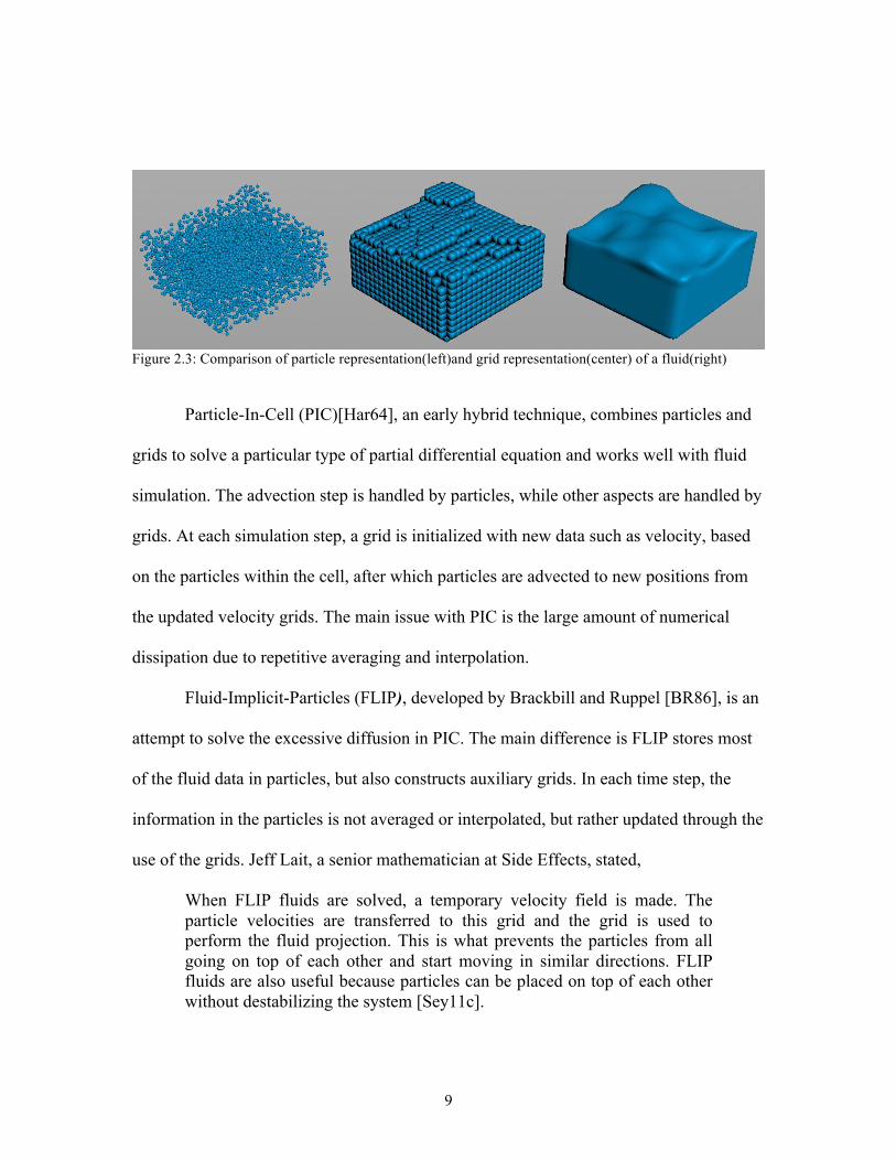
Grid-based Fluid Simulation, or the Eulerian viewpoint, in contrast to the

previous method, stores and tracks the physical information of the fluid in a fixed-point

grid. With this approach, numerical derivatives, such as pressure gradient and viscosity,

are easy to compute, yielding higher accuracy, but often suffer from mass loss. This

approach represents the smooth surface behavior of a fluid in an effective manner. Figure

2.3 shows the comparison of the particle representation and the grid representation of a

fluid.

9

Figure 2.3: Comparison of particle representation(left)and grid representation(center) of a fluid(right)

Particle-In-Cell (PIC)[Har64], an early hybrid technique, combines particles and

grids to solve a particular type of partial differential equation and works well with fluid

simulation. The advection step is handled by particles, while other aspects are handled by

grids. At each simulation step, a grid is initialized with new data such as velocity, based

on the particles within the cell, after which particles are advected to new positions from

the updated velocity grids. The main issue with PIC is the large amount of numerical

dissipation due to repetitive averaging and interpolation.

Fluid-Implicit-Particles (FLIP), developed by Brackbill and Ruppel [BR86], is an

attempt to solve the excessive diffusion in PIC. The main difference is FLIP stores most

of the fluid data in particles, but also constructs auxiliary grids. In each time step, the

information in the particles is not averaged or interpolated, but rather updated through the

use of the grids. Jeff Lait, a senior mathematician at Side Effects, stated,

When FLIP fluids are solved, a temporary velocity field is made. The particle velocities are transferred to this grid and the grid is used to perform the fluid projection. This is what prevents the particles from all going on top of each other and start moving in similar directions. FLIP fluids are also useful because particles can be placed on top of each other without destabilizing the system [Sey11c].

10

The FLIP solver was included in Houdini 11, released in 2010.

2.4 Rigid-Body Simulation in Computer Graphics

Rigid-body simulation techniques, used widely in the game and visual effects

industries, range from proprietary physics engines, such as PhysX by Nvidia [PhX14] and

Havok Physics by Havok [Hav14], to specialized multiphysics simulation libraries, such

as PhysBAM by Stanford [PhB14], to open-source solutions, such as Open Dynamics

[Ope07] Engine and Bullet Physics Engine [Rea14].

Bullet Physics Engine has become the most popular choice for more than half a

decade due to its robust convex hull collision detection, versatile constraint system

allowing easy art direction, and active open-source development community [BZC+11].

It was created by Erwin Coumans in 2006 with open-source Zlib licensing and mainly

used in game engines. The movie 2012, released in 2009, was a milestone for Bullet

Physics Engine in the visual effects community due to its impressive large-scale

destruction sequences created by Digital Domain (Figure 2.4). This movie marked the

first time Bullet Physics Engine had been adopted in such scale and detail in a feature

film. The potential of Bullet Physics Engine did not go unnoticed. Other visual effects

companies jumped onto the bandwagon and destruction sequences created with Bullet

Physics Engine showed up in films such as Inception, Prince of Persia, X-Men: First

Class, Deathly Hallows Parts 1 and 2 and more. Another key advantage of Bullet Physics

Engine is its open-source nature. Visual effects studios can access the low-level source

code, optimizing and integrating it into their existing destruction pipelines.

11

Figure 2.4: Los Angeles destruction in 2012created with Bullet Physics Engine © Columbia Pictures

2.5 Destruction Pipeline

Although the work of this thesis was performed with the Bullet Physics Engine

implementation in Houdini, the following destruction pipeline can generally be applied to

other rigid-body simulation techniques.

The three main stages of a destruction pipeline typically include:

i) Geometry Preparation Artists pre-fracture rigid-body objects. The Voronoi Diagram

shown in Figure 2.5is a popular fracturing technique because of its simple algorithm and

natural appearance in the final result. Featured points are created on the object either by a

random process or artistic control for a desired pattern; the object is then fractured at

locations equidistant from these featured points.

12

Figure 2.5: Voronoi Diagram with random feature points (left), and art-directed feature points(right)

Bullet Physics Engine utilizes convex hull collision detection for fast and robust

simulation. As a result, it does not handle concave objects effectively. Such concave

objects must be decomposed into smaller convex objects and glued together even though

they are used solely for collisions. Voronoi subdivision technique can also be used to

accomplish this goal (Figure 2.6).

13

Figure 2.6: A concave geometry fractured with Voronoi subdivision and grouped together

ii) Constraints and Choreography After being fractured, these small broken pieces are

connected together to define a constraint network. The constraints are usually

automatically generated, but artists can also add creative touches to define how the object

will be broken during the simulation. The destruction can then be animated or

choreographed based on the properties of the constraints. Properties such as strength (if

the object will be broken based on an impulse during the simulation time), and time until

active (control how the crack will progress), can be painted on the object by artists.

Figure 2.7 is an example of multi-level constraint networks used to choreograph

destruction of a house.

14

Figure 2.7: Example of multiple-level constraint networks used to choreograph destruction [BZC+11]

iii) Simulation and Rendering Fractured rigid-body objects and constraints are presented

in the simulation in low resolution for performance, either with point clouds or convex

hull objects depending on the implementation of the system and desired details in the

simulation result. Collision detection is divided into two phases of coarse-and-fast

broadphase and precise-and-slow narrowphase. Some acceleration structures, such axis-

aligned bounding boxes and convex hull bounding, are used in the broadphase. The glued

objects can also be presented with a single bounding object before they are broken apart.

The actual high-polygon-count fractured pieces can be used in narrowphase for better

details [BZC+11]. These low-resolution representations will be swapped with high-

resolution fractured pieces either after the simulation or during render time.

15

CHAPTER THREE

IMPLEMENTATION

The sand simulation work was created in Houdini 3D animation software, version

13.0.401. With the procedural nature of Houdini, countless possibilities exist to complete

a certain task. For the collapsing shot, the art direction prescribed the following sequence,

as depicted in Figure 3.1:

i) Break the sand mound into chunks, with

each chunk falling in succession for a few

beats; then, the rest of the mound will fall as

one piece.

ii) As each chunk falls, it will be broken

further into sand particles.

Although a good deal of trial-and-error

was involved in the development process of

this method, the only workflow presented is

the one that provided the best result and was

approved by the director.

Figure 3.1: Art keys of the collapsing sand by Rianti Hidayat

16

3.1 Workflow

A combination of rigid-body simulation and fluid simulation were used to create

the collapsing sand effects. The overall workflow (Figure 3.2) appears simple and

straightforward, but many small fine-tuning steps were required in each stage to achieve

proper timing and motion of the effects; these steps will be covered in the following

sections.

Figure 3.2: Workflow for creating collapsing effects

)UDFWXUH�3UHS

5LJLG�%RG\�6LP

)OXLG�3UHS

)OXLG�6LP

DFWLYH�5%'�REMHFWV

DFWLYH�IOXLG�REMHFWV

LQDFWLYH�5%'�REMHFWV

LQDFWLYH�IOXLG�REMHFWV

5HQGHUHG�DV�VDQG�FKXQNV

5HQGHUHG�DV�VDQG�SDUWLFOHVIOXLG�SDUWLFOHV

LQDFWLYH�5%'�IOXLG�REMHFWV�XVHG�DV�IOXLG�FROOLVLRQ�6')�YROXPHV

17

3.2 Fractures Preparation

Similar to the preparation required for other destruction scenes in visual effects

production, the original geometry in the scene needed to be pre-fractured for the desired

art-directed collapsing pattern. The Voronoi fracture technique was used to create

fractured geometries to feed into the rigid-body simulation. Feature points were scattered

on the surface of the geometry based on surface area, or scattered inside the geometry

based on volume density.

Figure 3.3: Voronoi fracture node in Houdini

Fracturing was automated by a Voronoi fracture node in Houdini shown in Figure

3.3, which could be used intuitively to determine how the geometry would be broken

apart. The result could be modified further by translating or rotating the feature point

18

group. The fractured pieces, however, often exhibited perfectly straight edges and

uniform sizes which were uninteresting from an artistic standpoint (Figure 3.4).

Figure 3.4: Uninteresting fractures with straight edges

To avoid such issues, the sand mound geometry was first separated into inner and

outer pieces. As observed from multiple videos references, when a sand mound collapses,

chunks of sand are usually peeled off in layers with the outermost chunks falling off first

(Figure 3.5).

19

Figure 3.5: Reference showing the outermost part will usually fall out of the sand mound first [San14b]

To achieve this goal, the inner piece of the sand mound geometry was first

subdivided into large chunks (Figure 3.6). This process was chosen largely due to artistic

decisions, since at the end of the collapse, all the sand would fall out of the shot at the

same time. Grouping these inner fractures into a small number of large pieces facilitated

a simpler and more effective approach.

20

Figure 3.6: Sand mound broken into outer piece (left) and inner piece (right)

For the outer piece of the sand mound geometry, the volume was broken into

small child pieces and large parent pieces in parallel. The child pieces were then grouped

together based on proximity to the parent pieces. The result was grouped chunks with

interesting imperfect edges (Figure 3.7). Later, the outer and inner fractures were

combined and ready to be simulated in the next stage. Figure 3.8 shows the resulting

Houdini network used for the fracture preparation stage.

21

Figure 3.7: Child pieces (bottom left) grouped together based on proximity to parents (top left)

22

Figure 3.8: Houdini network for the fractures preparation stage

23

3.3 Rigid-Body Simulation

Bullet Physics Engine was the preferred rigid-body solver for this work due to its

simplicity, performance and ease of control. The fractures were imported as inactive

rigid-body objects that were activated manually based on art direction. In this shot, the

coconut shell scraped the top of the sand mound; hence, the group of fractured pieces on

the top in contact with the coconut shell should be active first. After activation, the

objects were simulated with gravity and an additional nudging force. The remaining

inactive objects acted as collision objects until they were activated. Figure 3.9 shows the

rigid-body objects activation control network.

Figure 3.9: Rigid-body objects activation control network

24

Activation order was choreographed manually. A representation point encoded

with activation time was created for each parent group. The activation range was mapped

into a canonical space from zero to one and could be modified to tweak the simulation

result. These control points were imported to the simulation to activate the rigid-body

objects in a pre-designed destruction order as shown in Figure 3.10.

25

Figure 3.10: Activation order (left) and simulation result (right)

26

One problem with the Bullet Physics Engine was that collision detection could be

sensitive at times, causing the simulation to become explosive. In general, Bullet Physics

Engine works well with most destruction setups, but for this collapsing sand simulation,

the collision condition needed to be relaxed and revised with velocity modifications as

shown in Figure 3.11. The result from the rigid-body solver was cached, but some

additional preparation was needed before passing it to the fluid simulation.

Figure 3.11: Relaxing the collision condition inside the rigid-body simulation network

27

3.4 Fluid Preparation

Each parent group of the fractures was activated one-by-one, with geometries in

each group falling from the original sand mound geometry at the same time. Geometry

pieces associated with each group stayed together as rigid bodies at the beginning of the

fall, and gradually broke apart into sand particles. The continuity and timing of

converting each rigid-body into particles was crucial to the overall believability of the

effects. To blend the two states of the sand, each broken piece was fractured to even

smaller pieces. Particle activation time (not to be confused with rigid-body activation

time in a previous stage) was encoded into the new pieces. The new fluid activation time

was randomized from the moment the rigid-body was activated to a few frames later.

When a rigid-body object was activated to be converted to fluid particles, points

were scattered inside the geometry and fed into the fluid solver as a fluid particle source.

This newly created source emitted fluid particles to the fluid simulation in only a single

frame, and the original rigid-body object was simultaneously removed from the system to

avoid discontinuity. This workflow created nicely overlapped state transitions with the

illusion of sand chunks being cracked before broken into sand particles (Figure 3.13).

The Houdini network to control this technique is shown in Figure 3.14.

28

Figure 3.12: Inactive fluid object remaining as chunks (A’s), and active fluid objects turning to particles (B’s)

Figure 3.13: Houdini network of fluid preparation stage

3.5 Fluid Simulation

The Fluid Implicit Particle(FLIP) technique has been implemented as the main

fluid solver in Houdini software since version 11. In FLIP, fluid data is carried by

particles with auxiliary grids constructed in each time step to update the particle group

velocity. A few tweaks were applied to the standard FLIP simulation in Houdini to make

the particles behave like sand in this simulation.

29

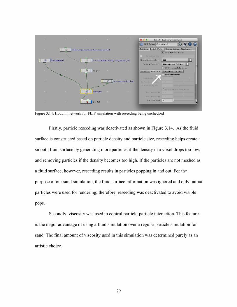
Figure 3.14: Houdini network for FLIP simulation with reseeding being unchecked

Firstly, particle reseeding was deactivated as shown in Figure 3.14. As the fluid

surface is constructed based on particle density and particle size, reseeding helps create a

smooth fluid surface by generating more particles if the density in a voxel drops too low,

and removing particles if the density becomes too high. If the particles are not meshed as

a fluid surface, however, reseeding results in particles popping in and out. For the

purpose of our sand simulation, the fluid surface information was ignored and only output

particles were used for rendering; therefore, reseeding was deactivated to avoid visible

pops.

Secondly, viscosity was used to control particle-particle interaction. This feature

is the major advantage of using a fluid simulation over a regular particle simulation for

sand. The final amount of viscosity used in this simulation was determined purely as an

artistic choice.

30

Figure 3.15: Inactive rigid-body objects and active fluid objects used as collision volumes in FLIP

Lastly, inactive rigid-body objects and active rigid-body objects that were not yet

transformed into fluid particles were brought into the fluid simulation as collision objects

(Figure 3.15). In early development, inactive objects were imported as fluid particles with

high viscosity for convenience and speed, but the result was not acceptable visually. An

effective way to handle collisions in FLIP was to convert rigid-body objects into signed

distance field volumes to be used in the velocity projection step. Converting objects to

volumes was computation-intensive and time-consuming, but collision handling was fast

and accurate.

3.6 Rendering

Rendering was divided into two parts: rendering rigid-body objects as sand

chunks, and rendering fluid particles as moving sand.

31

For sand chunks, dense particles were scattered inside rigid-body objects with

randomized sizes and colors. The scattering algorithm in Houdini worked well with static

objects, but scattered points changed position in each frame the base object moved. These

issues were resolved by first scattering points on a geometry component at rest. Once the

base geometry was moved, a transformation object was extracted by comparing the

moving geometry with the rest geometry, and this resultant transformation object was

applied to the scattered points. The transformation was handled by a lattice deformer

node inside Houdini (Figure 3.16).

Figure 3.16: Keeping fracturing and scattering particles consistent and avoiding pops with a lattice deformer For the moving sand, simulated particles were taken from the fluid simulation

with surface information removed. New size and color attributes were added to the

32

particles in a similar fashion to those on the sand chunks. Particles on sand chunks and

moving sand were then rendered as spheres with motion blur (Figures 3.17 and 3.18).

Figure 3.17: Randomizing color and size of the particles

Figure 3.18: Sand mound with uniform color and size (left) and randomized color and size (right)

33

3.7 Extra Sand Particles Finally, extra sand particles were simulated with a regular particle solver and

added on top of the sand mound when the coconut shell was moved and lifted (Figure

3.19).

Figure 3.19: Extra sand particles to be added on top of the collapsing sand effects

34

CHAPTER FOUR

RESULTS

To exhibit the function of each stage in the collapsing sand effects workflow, the

results from rigid-body and fluid simulations are separated in Figures 4.1 and 4.2. These

two figures can be compared to observe the timing of sand chunks being removed from

the rigid-body simulation and converted to sand particles in the fluid simulation

simultaneously. The two results were eventually seamlessly combined (Figure 4.3) and

rendered together for the final images in Figures 4.4a and 4.4b.

35

Figure 4.1: Result from rigid-body simulation

36

Figure 4.2: Result from fluid simulation

37

Figure 4.3: Combined result from rigid-body simulation and fluid simulation

38

Figure 4.4a: Final image from An Ode To Love (lighting pending)

39

Figure 4.4b: Final image from An Ode To Love (lighting pending)

40

CHAPTER FIVE

DISCUSSION AND FUTURE WORK

Although the collapsing sand effects were successfully accomplished, many

refinements could be made to the workflow. A short-term improvement would be to

simplify the system and package it into a single asset that could be reused for similar

effects in future productions. Other improvements include improving performance and

generalizing the technique.

5.1Easier Controls

The fine-tuning steps in the pipeline, such as destruction choreography, could be

controlled by more intuitive graphical means such as activating the rigid-body and fluid

objects with animated sphere primitives. This feature was originally part of the system

design, but due to lack of testing time, the early development of such visual controls

could not produce adequate results with precise timing, and were eventually replaced

with manual key-framing. With enough development time, the overall controls of the

system could be improved for frequent use by general artists without the need of going

through the underlying mechanics.

5.2 Better Performance

Heavy computation during the fluid simulation phase could be optimized,

mitigating hardware and time constraints. The current simulation required the full

41

capacity of a Hewlett-Packard HP Z620 workstation with dual socket3.30GHz Intel Xeon

E5-2643 processors and 32 GB of memory. Despite caching in various stages of the

pipeline, simulating and rendering the resultant animation still required up to six hours.

Many optimizations, such as automated domain resizing and occlusion culling, could be

implemented to further enhance performance, shortening the turnaround time for

practical everyday productions.

5.3 More Generalized Sand Solver

Ambitious future work for this project would be to research and develop a more

generalized sand solver that could handle various types and scales of sand effects. Many

early approaches to sand animation were specialized for certain types of sand phenomena

and some suffered from scaling. A potential technique that could be extended to handle

general sand effects is the material point method. Stomakhin et al. developed a material

point method to create realistic snow effects for the blockbuster feature animation,

Frozen[SSC+11] (Figure 5.1). Snow and sand have similar dual material properties,

namely both rigid-body and particle-like behaviors. A different extension of the material

point method could yield a robust generalized sand solver for any sand effect in digital

productions.

42

Figure 5.1: Result from A Material Point Method for Snow Simulation by Stomakhin et al. [SSC+11]

43

REFERENCES

[ABC+07] Christoph Ammann, Doug Bloom, Jonathan M. Cohen, John Courte,

Lucio Flores, Sho Hasegawa, Nikos Kalaitzidis, Terrance Tornberg, Laurence Treweek, Bob Winter, and Chris Yang. 2007. The birth of sandman. In ACM SIGGRAPH.

[Aur91] Franz Aurenhammer. 1991. Voronoi diagrams—a survey of a fundamental

geometric data structure. ACM Computing Surveys (CSUR), 23, 3, 345-405.

[BZC+11] Michael Baker, Nafees Bin Zafar, Mark Carlson, Erwin Coumans, Brice

Criswell, Takahiro Harada, and Phil Knight. 2011. Destruction and dynamics for film and game production. ACM SIGGRAPH Course Notes.

[BYM05] Nathan Bell, Yizhou Yu, and Peter J. Mucha. 2005. Particle-based

simulation of granular materials. In Proceedings of the 2005 ACM SIGGRAPH/Eurographics symposium on Computer animation. ACM, 77-86.

[BR86] J. U. Brackbill and H. M. Ruppel. 1986. FLIP: A method for adaptively

zoned, particle-in-cell calculations of fluid flows in two dimensions. Journal of Computational Physics, 65, 2, 314-343.

[BM07] Robert Bridson and Matthias Müller-Fischer. 2007. Fluid simulation:

SIGGRAPH 2007 course notes. ACM SIGGRAPH 2007 courses, 1-81. [Fai09] Ian Failes. 2009. 2012: Disaster Porn. (November 2009). Retrieved July

16, 2014 from http://www.fxguide.com/featured/2012_Disaster_Porn/. [Har64] F. H. Harlow. 1963. The particle-in-cell method for numerical solution of

problems in fluid dynamics. In Experimental arithmetic, high-speed computations and mathematics.

[Hav14] Havok Physics | Havok. Retrieved July 16, 2014 from

http://www.havok.com/products/physics. [Mon92] J. J. Monaghan. 1992. Smoothed particle hydrodynamics. Annual review

of astronomy and astrophysics, 30, 543-574. [Ope07] Open Dynamics Engine. (May 2007). Retrieved July 16, 2014 from

http://www.ode.org/.

44

[PhB14] PhysBAM. Retrieved July 16, 2014 from http://physbam.stanford.edu/. [PhX14] PhysX | GeForce. Retrieved July 16, 2014 from

http://www.geforce.com/hardware/technology/physx. [Rea14] Real-Time Physics Simulation. (May 2014). Retrieved July 16, 2014 from

http://bulletphysics.org. [San14a] SandCastle Collapse at San Francisco. Video. (July 2009). Retrieved July

16, 2014 from https://www.youtube.com/watch?v=Lyh3oiRO1ls. [San14b] Sand Castle Destruction 2011. Video. (July 2011). Retrieved July 16, 2014

from https://www.youtube.com/watch?v=CTzzxSx0U2E. [Sey11a] Mike Seymour. 2011. Art of Destruction (or Art of Blowing Crap Up).

(December 2011). Retrieved July 16, 2014 from http://www.fxguide.com/featured/art-of-destruction-or-art-of-blowing-crap-up/.

[Sey11b] Mike Seymour. 2011. Bullet Open Source Physics Engine. (January

2011). Retrieved July 16, 2014 from https://www.fxguide.com/featured/bullet_open_source_physics_engine/.

[Sey11c] Mike Seymour. 2011. The Science of Fluid Sims. (September 2011).

Retrieved July 16, 2014 from http://www.fxguide.com/featured/the-science-of-fluid-sims/.

[SSC+13] Alexey Stomakhin, Craig Schroeder, Lawrence Chai, Joseph Teran, and

Andrew Selle. 2013. A material point method for snow simulation. ACM Transactions on Graphics (TOG), 32, 4, 102.

[ZB05] Yongning Zhu and Robert Bridson. 2005. Animating sand as a fluid. In

ACM Transactions on Graphics (TOG). ACM, 965-972.