Getting a Hand By Cutting Them Off: How Uncertainty over

Political Corruption Affects Violence∗

Paul Zachary† William Spaniel‡

July 15, 2015

Abstract

What role do politicians have in bargaining with violent non-state actors to determine

the level of violence in their districts? Although some studies address this question in the

context of civil war, it is unclear whether their findings generalize to organizations that

do not want to overthrow the state. Unlike political actors, criminal groups monopolize

markets by using violence to eliminate rival firms from the marketplace. We argue that

increased tenure in political office increases cartels’ knowledge about local political elites’

willingness to accept bribes. With bribes accepted and levels of police enforcement low,

cartels endogenously ratchet up levels of violence. We formalize our claims with a model

and then test its implications with a novel dataset on violent incidents and political tenure

in Mexico. For one additional year of political tenure, the sum of this effect across all

municipalities is an additional 2,300 homicides per year.

∗Previous version of this paper were presented at the Midwest Political Science Association, InternationalStudies Association, and Western Political Science Association conferences as well as seminars at UC Riverside;UCLA; and Rochester. We thank Sergio Ascencio, Regina Bateson, Peter Bils, Kevin Clarke, Jesse Driscoll,Kent Eaton, James Fowler, Matthew Gichohi, Thad Kousser, David Lake, Benjamin Laughlin, Alexander Lee,Ben Lessing, Brad LeVeck, John Patty, Aila Matanock, Will Moore, MaryClare Roche, Phil Roeder, ArturasRozenas, Emily Sellers, Branislav Slantchev, Brad Smith, Barbara Walter, and Michael Weintraub for theirfeedback. We are indebted to Rzan Akel, Andrea de Barros, and Jacob Boeri for excellent research assistance.Zachary acknowledges research support fron the National Science Foundation and the Robert Wood JohnsonFoundation. All errors remain the authors’ own.†PhD Candidate, Department of Political Science, University of California, San Diego, 9500 Gilman Drive,

#0521, La Jolla, CA 92093 (pzachary@ucsd.edu)‡PhD Candidate, Department of Political Science, University of Rochester, Harkness Hall 333, Rochester,

NY 14627 (williamspaniel@gmail.com, http://williamspaniel.com).

1 Introduction

Following a decade of research on civil war onset and duration, the local dynamics of political

violence is an increasingly popular topic for scholars. Beyond coercing states into making

concessions and providing information about both sides’ resolve, violence provides armed

groups with a number of strategic benefits (Pape 2003; Cohen 2014; Weinstein 2007).1 Despite

these incentives, most conflicts exhibit substantial subnational variation in the intensity of

violence. Scholars have hitherto focused on variation in armed group’s military capabilities,

advantageous terrain, or the intensity of local grievances to explain this variation (Cederman,

et al. 2011; Buhaug and Gates 2002).

In this paper, we identify an alternate mechanism: political corruption. An increasing

number of violent conflicts are not direct attempts to overthrow the state. Instead, they

are among criminal organizations for control of criminal extraction.2 In such conflicts, a

substantial portion of violence is not directed at the state but instead at rival cartels. We

show that cartels in these instances use bribery as a strategy to reduce police enforcement to

maintain their local monopoly on crime. To do so, we develop a formal model of the bargaining

process between political elites and cartels over the level of police enforcement in a district.

In our model, a local cartel attempts to reduce that enforcement by offering a bribe to local

political elites. Elites then weigh their desire to minimize violence against bribery’s monetary

benefit. Finally, the local cartel uses violence—endogenously determined—to maintain control

of valuable territory against a rival cartel.

Uncertainty plays a critical role in determining the outcome of the interaction and thus

helps explain subnational variation. When the cartel knows the politician’s level of corruption,

it can choose a precise bribe and ensure that enforcement will be lax. Consequently, levels

of violence rise. In contrast, when the cartel faces great uncertainty about the politician’s

corruptibility, it may offer smaller bribes that risk being rejected by the politician. This time,

we expect levels of violence to be comparatively lower because the politician is more likely to

enforce the laws. Thus, counter to standard models of costly conflict, we expect uncertainty

to decrease levels of violence.

We then argue that regions where local political machines have more recently taken con-

trol will see lower levels of violence. This might seem counterintuitive because experience

seemingly should increase skill and thus decrease violence. Indeed, standard theories of ret-

1More specifically, violence can prevent civil defection and maintain territorial control (Kalyvas 2006), forcecivilians to contribute rents to armed groups (Weinstien 2007; Humphreys and Weinstein 2006), and improveunit cohesion and esprit de corps (Cohen 2014).

2In this paper, we use data from the ongoing Drug War in Mexico. Other examples include gang violence inthe United States as well as Central and South America (Kronick 2014) and drug smuggling in the Caribbeanand West Africa.

1

rospective voting would predict the opposite (Fiorina 1981; Kinder and Kiewiet 1979, 1981),

and Cummins (2009) finds that American governors and their parties suffer at the polls for

high crime rates. The model indicates that the expected negative correlation makes sense

when levels of corruption are low, as in the United States. Leaders simply cannot serve for

long if they are ineffective.

However, the model also shows that a positive correlation can exist when levels of cor-

ruption are generally high. Drawing from recent theoretical and empirical conceptualizations

of uncertainty (Wolford 2007; Rider 2013), we argue that cartels know less about leaders’

preferences earlier in political tenure. Cartels facing greater uncertainty are more likely to

see their offers fail, leading to properly enforced laws and less violence. As tenure progresses,

though, the cartels can better narrow their suppositions about leader preferences. Bribery is

more likely to succeed here, leading to laxly enforced laws and more violence. Thus, although

retrospective voting may hurt a corrupt political party to some degree, our empirical results

suggest that the uncertainty effect predominates.

In sum, our model shows that attempts to understand criminal behavior by treating gov-

erning institutions as mere bystanders misses important bargaining dynamics. By focusing

on political corruption and institutions, we contribute to an expanding literature in the polit-

ical economy of development and political violence. Due to their coding rules, most previous

studies of civil war restrict their analysis to contestation among armed groups over control

of state institutions.3 Paradoxically, this excludes one of the most common and destructive

forms of political violence: conflict between criminal organizations.4 We choose to model

the effect of institutions on violence because actors in these conflicts leave many institutions

intact, which could impact the conflict process. Whether this is the case, and the mechanism

through which these effects might occur, is currently little understood. Further, we focus on

bribery to explore another key difference between criminal and civil wars: nearly unlimited

access to rents. As we demonstrate below, criminal groups likely prefer to bribe politicians

than fight them as a profit-maximizing strategy (Weinstein 2007).

We draw evidence from the drug war in Mexico to test our model’s empirical implications.

Using data from the Office of the President from 2000 to 2011 on all extralegal deaths reported

to Mexican police, we show that political tenure is positively correlated with a district’s murder

rate and this result is robust to a variety of model specifications. The estimated marginal

effect of an additional year of tenure in Congress is associated with one additional death in

3For more on these rules, see Sambanis 2004 and Singer and Small 1982.4Although their internal dynamics are less studied that civil wars, criminal violence currently affects a

number of developing countries throughout the world. Particularly violent examples include the ongoing drugwars in Mexico and Colombia and gang violence in Brazil, Venezuela, and Central America (Rios 2012; Osorio2013; Kronick 2014).

2

every municipality in our dataset. Although every murder is tragic, one additional death might

seem substantively insignificant. Across all 2,371 municipalities in our dataset, each additional

year of tenure increases Mexico’s homicide rate by the the same number. Substantively, this

increase is equivalent to the total number of homicides committed in 2011 in France, Germany,

the United Kingdom, the Netherlands, and Belgium combined (UNODC 2014). This finding

shows that criminal violence is neither apolitical nor is national enforcement policy a sufficient

explanation of this subnational variation (Resa Nestares 2001; Sabet and Rios 2009, 5-12;

Osorio 2013).

Our argument differs from prior work on criminal violence in several key regards. First,

by focusing on subnational variation, we control for changes in enforcement priorities set by

the President and international donors. In the case of Mexico, several scholars use the anti-

cartel rhetoric and refusal to accept bribes among presidents elected since 2000 to explain

the increase in violence (Resa Nestares 2001; Sabet and Rios 2009, 5-12; Osorio 2013). While

this certainly increased violence nationally, the preferences of the president cannot explain

subnational variation in levels of violence. Second, by modeling the strategic interactions

between politicians and cartels, we explore how politicians can create conditions that are

conducive to increases in violence. Accounting for variation in the level of corruption among

political elites, we stand apart from prior research that assumes that law enforcement and

politicians always pursue cartels (Rios 2013, 2014).

That bribery is an effective strategy for violent actors has several implications for our

understanding of conflict processes and economic development. We show that political elites

can determine the level of violence within their district. While the literature on the political

economy of development has long emphasized the role elites have in supporting economic

growth and improving public health, we know relatively little about how rent-seeking behavior

affects normatively bad outcomes (Keefer and Knack 1997; Clague, et al. 1996). As civil war

disincentives economic investment and destroys property rights, local violence is a poverty trap

(Varese 2011; Dell Forthcoming; Acemoglu, et al. 2001; Collier, et al. 2003). Our empirical

results, moreover, suggest that competitive elections do not ameliorate this problem. Instead,

strong domestic anti-corruption agencies must credibly threaten politicians from accepting

bribes and allowing violence. This has important implications not just for Latin America,

but even highly developed states such as the United States that have large criminal gang

problems.

These results also have implications for our understanding of clientelism. Previous work

on this topic typically focuses on the strategies politicians employ to influence elections and

vote choice (Stokes 2005; Gans-Morse, et al. 2014). As elections do not reflect the true will

of the people, clientelism inverts the accountability between politicians and voters. Yet, the

3

American literature on lobbying and campaign donations shows that money is a powerful tool

that influences politicians’ behavior (Bonica 2014; Romer and Snyder 1994). Surprisingly little

research applies this insight into understanding politicians’ incentives in new democracies. We

show here that even if voters use elections to hold politicians accountable for crime, cartels

can still use bribery to influence policy decisions. This shows that clientelist relationships can

occur both between politicians and voters as well as politicians and financial interests.

This paper proceeds as follows. We begin by introducing our formal model of an interaction

between two cartels and a local politician. Second, we test the empirical implications of

the model using a novel dataset of violence and voting patterns. Finally, we conclude with

suggestions for future research.

2 The Model

The game consists of three players: two cartels (denoted 1 and 2) and a local party.5 Cartel

1 has status quo control over the local district (standardized to value 1) and needs to use

violence to keep Cartel 2 from encroaching on its territory. Cartel 2, meanwhile, can use

violence to challenge Cartel 1’s control. The party wishes to keep the level of violence down,

though it is willing to permit violence at the right price.

Play begins with Cartel 1 taking advantage of its regional ties and familiarity to offer a

bribe b ≥ 0 the party to limit the enforcement of anti-violence laws. If the party accepts the

bribe, the party implements a “no enforcement” policy of α = α, where α ∈ (0, 1) reflects

Cartel 1’s comparative advantage at producing violence relative to Cartel 2.6 In exchange,

Cartel 1 pays b to the party.7 To analyze how the outcome varies as a function of the party’s

level of corruption, the party internalizes bc from the bribe payment, where c > 0. Thus,

higher levels of c reflect higher levels of corruption; in turn, increasing c indicates that a

politician increasingly values monetary bribes over sound public policy.

5Although we ultimately care about police enforcement, we focus on party-level bribery because such large-scale corrupt behavior requires political consent, and these party leaders ultimately have control over policepolicies.

6Thus, higher levels of enforcement erode Cartel 1’s territory control of the territory, allowing Cartel 2 toencroach (Osorio 2013). An alternative interpretation is that our game is an approximation of a game in whichthe status quo actor has closer ties to the local political party, which appears generally true across Mexicanmunicipalities. Thus, we focus on bargaining over selective enforcement at the local level rather than generalenforcement of laws that federal troops tend to administer.

7We are therefore analyzing a bargaining game with quid-pro-quo offers. This might seem strange given thatthe very nature of bribery means that such deals are not enforceable through traditional legal mechanisms.However, we could instead think of this game as the reduced form of a longer-horizon exchange. Rather thanpaying the entire bribe up front, the cartel could make a number of smaller payments over time. Given thisrepetition, the party would not have incentive to defect on the deal when doing so would cancel the long-termgains from cooperation (Axelrod 1984). As such, another interpretation for the bribe value b is the total valueof a large string of small bribes.

4

If the party rejects, it selects a level of enforcement α ∈ [α, 1). However, exerting such

effort is costly. To reflect the enforcement cost, the party pays k(α), a function that is

differentiable everywhere on the unit interval and where −k′(α) > 0 and −k′′(α) ≤ 0. This

intuitively implies that effort harms Cartel 1’s ability to commit violence but is costly to the

party.

Both cartels see the level of enforcement and simultaneously choose respective levels of

violence v1 ≥ 0 and v2 ≥ 0. A contest success function uses the violence levels to determine

the distribution of the district at the end of the game.8 Specifically, Cartel 1 takes v1v1+v2

portion and Cartel 2 takes the remainder, or v2v1+v2

.9 Each pays a cost for its effort. We

therefore subtract v2 from Cartel 2’s payoff and αv1 from Cartel 1’s payoff.

Recapping, the timing is as follows:

1. Cartel 1 offers a bribe b to the party

2. The party accepts or rejects the bribe

3. If the party rejects the bribe, it sets a level of enforcement

4. The cartels simultaneously set violence levels v1 and v2

5. Payoffs are realized

Note that we make very few restrictions on the players’ choices. The bribe, level of police

enforcement, and levels of cartel violence are all endogenously selected; only the accept/reject

choice is a binary decision. This helps ensure that the theoretical results we obtain are not a

consequence of restrictive modeling decisions but instead the optimal strategies of the players.

Overall, those payoffs are as follows. If the bribe fails, the party suffers the total amount

of violence minus its effort to reduce violence, or −(v1 + v2)− k(α). If the bribe succeeds, the

party still suffers the total amount of violence but gains the value of the bribe multiplied by

c > 0. Formally, this is −(v1 + v2) + bc. Thus, another way to interpret c is how much the

party weighs self-enrichment to good policy. Cartel 1 receives v1v1+v2

− αv1 minus its bribe (if

accepted), while Cartel 2 earns v2v1+v2

− v2.

8We thus assume that the cartels are already engaged in costly conflict at the start of the interaction. Whilethis allows us to focus on the bargaining dynamics between cartels and politicians, one might imagine that weare studying a reduced-form game.

9One might imagine that enforcement does not hurt Cartel 1’s comparative advantage in violence but ratherdirectly diminishes its ability to win the contest. We have analyzed such a model. The results are there aresimilar but stronger than those we present here.

5

Table 1: Notation of the bribery game

Notation Description

vi Cartel i’s weakly positive level of violenceα Cartel 1’s relative advantage in producing violencek(α) Party’s strictly decreasing cost of enforcement functionc Party’s strictly positive level of corruptionb Cartel 1’s weakly positive bribe to the party

2.1 Assumptions

Our model has five key assumptions, which we support qualitatively in this section. Our

first assumption is that multiple cartels do not always peacefully coexist. Unlike traditional

firms, cartels lack formal dispute resolution mechanisms like the courts. This is because the

possession, sale, and/or distribution of narcotics is illegal under Mexican law. When disputes

arise, or a rival cartel attempt to enter a new market, the existing cartel can only use violence

to defend its market (Miron 1999). Despite the lack of property rights, cooperation might

still be possible given the right incentives. Indeed, cartel leaders sometimes form temporary

alliances and cooperate with one another.10 The need to monopolize smuggling routes into

the United States makes any such cooperation epiphenomenal. In sum, cartels routinely use

violence to compete for territory.

Second, we assume that cartels do not know the ex ante corruptibility of local political

elites. In other words, a politician’s corruptibility is an innate quality that is difficult to suss

out. Politicians, moreover, have incentives to misrepresent their willingness to take bribes to

maximize a cartel’s offer and improve their perception among the public. As an example of

such misrepresentation, Andres Granier was governor of Tabasco until 2012. During his time

in office, Granier was not generally seen as corrupt. This changed in 2013, when a local radio

station leaked recording of a conversation where he claimed to own enormous quantities of

designer clothing (Zabludovsky 2013a). Later arraigned on tax evasion, Granier is alleged

to have diverted $156 million in federal funds from the state budget (Castillo 2013). This

example suggests that corruptibility is a latent personality trait that is not apparent to voters

or cartels.

Third, we assume that police enforcement increases the costs of territorial competition.

10Many of these, however, are relatively short lived. The story of Juarez Cartel leader Vincente CarrilloFuentes is emblematic. Carrillo formed an alliance with the Sinaloa cartel early in the 2000s. When the headof the Sinaloa cartel killed Carrillo’s borther in 2004, the alliance ended (Associated Press 2014; Beittel 2011,10).

6

Consider when police confiscate large portions of a cartel’s profits in raids. Without access

to this cash, a cartel is in a worse position to bribe officials, purchase weapons, and pay its

workers. Alternatively, more enforcement means more arrests, forcing a cartel to train new

recruits and increase hazard pay to meet that demand. Either way, a local cartel would expect

to pay more to maintain its control.

Fourth, we assume that political elites can influence the deployment and enforcement prior-

ities of police and security forces. There are three principle police forces in Mexico: the Policıa

Federal (PF), state, and local police forces. Political elites can influence policing decisions

at all levels of government through encouraging corruption at the Attorney General’s office,

among police chiefs, and even by directly ordering police officers to ignore drug trafficking

(GAO 1996, 9; Sullivan and Elkus 2008). For example, the former governor of Quintana Roo

state, Mario Villanueva Madrid, was sentenced to almost eleven years in American prison

for conspiracy to launder millions of dollars in bribes (Zabludovsky 2013b). According to

prosecutors, “Mr. Villanueva had agreed to let the Juarez cartel. . . transport cocaine from

Colombia through Quintana Roo and on to the United States in exchange for up to $500,000

per shipment. Traffickers were free to unload drug shipments at a state government hangar

of a local airport” (Zabludovsky 2013b). As a clandestine activity, we cannot directly prove

collusion between politicians and cartels. However, the number of arrests of high-ranking

politicians suggests that these are not isolated incidents.

Finally, to obtain any variation empirically, parties must be willing to reject low bribes.

One potential issue here is that cartels can threaten violence against politicians and force them

to accept even minimal amounts or risk death. Although cartels have assassinated numerous

politicians over the course of the drug war, such a strategy appears to be ineffective at reducing

local enforcement. For example, after the Knights Templar (allegedly) assassinated mayor of

Santa Ana Maya Ygnacio Lopez Mendoza, President Felipe Calderon deployed federal troops

to combat cartel activity in the area. So while assassinations may remove troublesome party

officials from power, they may ultimately create a worse problem. Bribery thus appears to be

a cheaper option.

2.2 Complete Information Equilibria

Since this is an extensive form game with complete information, we solve for its subgame

perfect equilibria. SPE require that all strategy choices are sequentially rational, ensuring

that players can only carry out threats that they have incentive to follow through on.

Proposition 1. If the party’s level of corruption is sufficiently high, Cartel 1 and the party

reach an agreement. In the unique SPE for these parameters, violence levels are high. If the

7

party’s level of corruption is sufficiently low, no mutually acceptable bribe exists. In all SPE

for these parameters, violence levels are low.

See the appendix for a complete proof. There are two phases to analyze: bribery and

violence. First, consider the violence subgame with varying levels of enforcement. Standard

with contest success functions, each party produces non-zero violence in equilibrium because.

Moreover, because Cartel 1 has a lower marginal cost for violence on its territory (which α

reflects), Cartel 1 produces more violence than Cartel 2, ensuring that it expects to win more

of the prize at the end. Based on these predicted levels of violence, the party chooses a level

of enforcement that optimizes its tradeoff between reducing the effectiveness of violence and

exerting effort, which we call α∗.

That optimal level of enforcement lingers throughout the game. Critically, enforcement

erodes Cartel 1’s status quo advantage over Cartel 2, giving it incentive to bribe the party and

secure a greater share of the good through the contest. This issue impacts the other phase:

bargaining between Cartel 1 and the party. Anticipating how various levels of enforcement

affect its ability to capture rents, Cartel 1 can calculate its marginal gain for buying the party’s

compliance. Meanwhile, knowing the party’s level of corruption and desire to reduce violence,

Cartel 1 can calculate the party’s minimally acceptable bribe and convert it to a monetary

value. If the value to Cartel 1 is greater than the party’s minimally acceptable bribe—

because the party’s level of corruption is sufficiently high—then a bargaining range exists.

Because Cartel 1 has all the proposal power, it chooses a bribe exactly equal to the minimally

acceptable amount, and negotiations succeed. The party subsequently shirks on enforcement.

If the value to Cartel 1 is less than the party’s minimally acceptable bribe—because the

party’s level of corruption is sufficiently low—then the bargaining range disappears.

Although enforcement is higher when the bribe succeeds, it remains unclear how agreement

affects observed violence. Despite the higher costs of violence, Cartel 1 might overcompensate

for the disadvantage. Alternatively, Cartel 2 might endogenously increase its violence to

exploit Cartel 1’s weakness. The following remark addresses that:

Remark 1. Levels of violence are higher when Cartel 1’s bribe succeeds than when it fails.

The appendix provides a detailed explanation. Regardless, for any given α, the optimal

levels of violence for the respective states are v∗1 = 1(1+α)2

and v∗2 = α(1+α)2

. Recall that, in

equilibrium, the party’s optimal level of enforcement is α∗, which is greater than α. As a

result, Cartel 1’s violence decreases with enforcement but Cartel 2’s increases. However, the

decreasing effect on Cartel 1 dominates the increasing effect on Cartel 2, meaning that overall

violence diminishes when with enforcement.

8

c∗

11+α

11+α∗

Level of Party Corruption

Equ

ilib

riu

mV

iole

nce

Rea

lize

d

Figure 1: Equilibrium levels of realized violence by the level of party corruption. Whencorruption is below the critical threshold c∗, the cartel finds bribery too expensive. Violencesubsequently diminishes. When corruption is high, the bribe succeeds, resulting in higherlevels of violence.

While this complete information game generates baseline results, it makes a strong as-

sumption about the bargaining phase of the game: Cartel 1 knows the party’s exact level of

corruption. It can then select the appropriate offer to the party and reap the entire surplus.

In practice, though, it would be difficult for a cartel to know the exact amount it needs to

offer a party to buy its compliance. After all, although levels of corruption correlate with

many observable factors like platform and reputation, the precise level is an internal attribute

of party officials. Thus, a more plausible setup would make Cartel 1 uncertain about party’s

minimally acceptable bribe. We investigate this scenario below.

2.3 Uncertainty about Corruption

Consider the following modification to the game. Nature now begins by drawing a level of

corruption of the party as one of two types.11 Specifically, the party is more corrupt with

probability p while the party is less corrupt with probability 1 − p. These varying levels of

corruptibility influence the intrinsic value of the bribe to the party. Thus, holding a bribe

level fixed at b, a more corrupt type values that bribe at bc′ whereas a less corrupt type

11Similar results would follow in an interaction where the party’s level of corruption from a continuum oftypes.

9

values it at bc, with c′ > c. In words, less corrupt types find bribes to be less valuable

peso for peso. Because corruptibility is an internal attribute, it is private information to the

party. The cartels therefore only know the prior at the start of the game. This prior may

be strong or weak based on observable factors that correlate with corruptibility, and we will

eventually investigate how the game’s equilibria change as a function of the extent of Cartel

1’s uncertainty.

Since the interaction is now a sequential game with incomplete information, we search for

its perfect Bayesian equilibria (PBE). A PBE is a set of strategies and beliefs such that the

strategies are sequentially rational and players update their beliefs via Bayes’ rule wherever

possible. Although this type of incomplete information game often yields multiple equilibria

depending on off-the-path beliefs that cannot be derived from Bayes’ rule, the outcomes we

present here are unique. This is because the cartels’ uncertainty about the party’s level of

corruption only has payoff-relevant ramifications during the accept/reject phase of the game.

However, the actor facing uncertainty (Cartel 1) makes an offer before the informed actor

(the party) decides how to respond. Consequently, the cartels need not analyze signals before

moving.

We begin with the case in which uncertainty proves irrelevant:

Proposition 2. For c′ sufficiently small, bargaining between Cartel 1 and the party fails with

certainty. Equilibrium levels of violence are low.

The logic follows straight from the complete information analysis; thus, we omit a full

proof. If the most corrupt type is not particularly corrupt, then no bargaining range exists.

In turn, Cartel 1 offers an amount insufficient to reach an agreement. But if Cartel 1 is

unwilling to buy off the more corrupt type, it certainly is unwilling to buy off a less corrupt

type too.

As such, information only matters in cases where corruption is generally high. We therefore

focus the remainder of our analysis on situations in which both types would be willing to

accept the largest bribe Cartel 1 would be willing to offer.12 This is also the most interesting

case substantively. Based on our above qualitative discussion above, local officials and cartels

seem willing to negotiate agreements with one another. Stories and criminal proceedings

of corruption and collusion between cartels and officials are not limited to any particular

geographic region, political party, or socioeconomic background. With bribery so prevalent,

we focus on that particular parameter condition.

12Another case exists in which a bargaining range exists only for the more corrupt type. Here, Cartel 1 cansimply focus on settling with the more corrupt type. However, uncertainty is not relevant here. Under suchconditions, the different types could credibly separate in a cheap talk extension to the game. This is becausethe less corrupt type, even with complete separation, receives the same offer as it would with all informationrevealed.

10

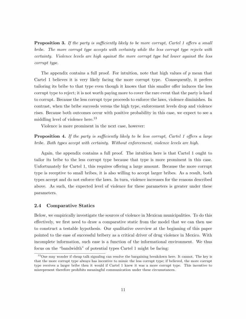
Proposition 3. If the party is sufficiently likely to be more corrupt, Cartel 1 offers a small

bribe. The more corrupt type accepts with certainty while the less corrupt type rejects with

certainty. Violence levels are high against the more corrupt type but lower against the less

corrupt type.

The appendix contains a full proof. For intuition, note that high values of p mean that

Cartel 1 believes it is very likely facing the more corrupt type. Consequently, it prefers

tailoring its bribe to that type even though it knows that this smaller offer induces the less

corrupt type to reject; it is not worth paying more to cover the rare event that the party is hard

to corrupt. Because the less corrupt type proceeds to enforce the laws, violence diminishes. In

contrast, when the bribe succeeds versus the high type, enforcement levels drop and violence

rises. Because both outcomes occur with positive probability in this case, we expect to see a

middling level of violence here.13

Violence is more prominent in the next case, however:

Proposition 4. If the party is sufficiently likely to be less corrupt, Cartel 1 offers a large

bribe. Both types accept with certainty. Without enforcement, violence levels are high.

Again, the appendix contains a full proof. The intuition here is that Cartel 1 ought to

tailor its bribe to the less corrupt type because that type is more prominent in this case.

Unfortunately for Cartel 1, this requires offering a large amount. Because the more corrupt

type is receptive to small bribes, it is also willing to accept larger bribes. As a result, both

types accept and do not enforce the laws. In turn, violence increases for the reasons described

above. As such, the expected level of violence for these parameters is greater under these

parameters.

2.4 Comparative Statics

Below, we empirically investigate the sources of violence in Mexican municipalities. To do this

effectively, we first need to draw a comparative static from the model that we can then use

to construct a testable hypothesis. Our qualitative overview at the beginning of this paper

pointed to the ease of successful bribery as a critical driver of drug violence in Mexico. With

incomplete information, such ease is a function of the informational environment. We thus

focus on the “bandwidth” of potential types Cartel 1 might be facing:

13One may wonder if cheap talk signaling can resolve the bargaining breakdown here. It cannot. The key isthat the more corrupt type always has incentive to mimic the less corrupt type; if believed, the more corrupttype receives a larger bribe then it would if Cartel 1 knew it was a more corrupt type. This incentive tomisrepresent therefore prohibits meaningful communication under these circumstances.

11

Proposition 5. If mutually acceptable bribes exist for both types, violence is weakly increases

as uncertainty about the party (i.e., c′ − c) decreases.

Once more, the appendix contains the full proof. The basic intuition is as follows. Without

uncertainty, per Proposition 1, Cartel 1 can appropriately tailor the bribe and reach a mutually

preferable settlement with the party. In the incomplete information case, the bandwidth of

types (c′ − c, or how different the types are compared to one another) is one measurement

of uncertainty. As that bandwidth diminishes, the potential types the cartel could be facing

become increasingly similar. This helps Cartel 1 find an offer that both would prefer to

bargaining breakdown.

Essentially, Cartel 1 faces a risk-return tradeoff. Broadly, it has two options. First, it can

offer small amount, hope that it is actually facing the more corrupt type, and suffer through

full enforcement against the less corrupt type. Second, it can offer a large amount and induce

both types to accept. This second case is expensive because it requires paying the large bribe

to both types, effectively costing Cartel 1 some fixed amount whenever the party is the more

corrupt type. However, as c′−c goes to 0, the risk premium Cartel 1 pays becomes vanishingly

small. As such, the amount “wasted” on the bribe to the corrupt type becomes increasingly

insignificant. In turn, Cartel 1 prefers offering the amount necessary to induce both types to

accept.14

Although reducing uncertainty leads to an increase in the likelihood of settlement, note

that it leads to an increase in the level of violence. This should be striking to researchers

familiar with bargaining and conflict. Normally such models show that reducing uncertainty

reduces conflict. On a technical level, this remains true here: the level of observed conflict (i.e.,

bargaining breakdown) between Cartel 1 and the party decreases as uncertainty decreases.

However, the purpose of an agreement between the two is to increase the effectiveness of

violence for Cartel 1. As such, decreasing uncertainty has a negative externality on outsiders

(i.e., private citizens) who want a decrease in the level of violence.

Before moving on, it is worth highlighting that this is a comparative static on how bargain-

ing patterns change when information exogenously improves. This is useful because dominant

cartels can shift over time. Nevertheless, one may reasonably wonder whether the same effect

would hold if information endogenously improved through a repeated offers bargaining setup.

Indeed, through a process similar to “convergence” (Slantchev 2003), it does. Since such a

model is substantially more complicated and yields comparable results, we choose to focus on

the one above.14Note that Proposition 5 is a conditional statement. If the bargaining range is empty for one type but not

the other, decreasing uncertainty could push the bribable type across c∗ threshold, which in turn decreasesviolence. Due to the prevalence of corruption, we choose to focus on the case where both levels of corruptionare greater than c∗.

12

3 Empirics

This section introduces our dataset on violent events and political tenure in Mexico. We

discuss our model of the effect of tenure on violence and conclude by presenting our results.

3.1 Hypothesis

Before delving into the data, we must first derive a testable implication from the model.

The formal analysis demonstrates that high-quality information is critical for the parties to

reach an agreement. This presents a major problem for empirical inquiry, however. Perfectly

predicting bargaining failure would require the analyst to know more than the parties in the

interaction. After all, if breakdown were perfectly predictable for the actors involved, the

cartel would simply increase its offer to an acceptable level and eliminate any inefficiency.

Thus, inevitably, bargaining breakdown (and thus variation in violence) is in the error term

(Gartzke 1999).

Fortunately, despite this hurdle, fruitful inquiry is still possible. Rather than assume that

researchers can better understand the information asymmetry than the players involved, we

can instead investigate environments that correlate with uncertainty in general. Recall that

Proposition 5 measures such uncertainty using the “bandwidth” of possible types. Relating

this to observable factors, Wolford (2007) argues that new leadership creates a shock to

informational structures. Opposing actors must throw out their estimates of the old leader’s

resolve and begin the intelligence process anew. However, as a leader’s tenure increases,

those estimates become progressively better and therefore the bandwidth of possible types

decreases. Bargaining is more likely to succeed under these circumstances.

That said, Proposition 2 indicates that information only matters in areas where corrup-

tion is high in general. In places where corruption is normally low—highly function Western

democracies, for example—we would expect tenure to matter little in this regard. In contrast,

we would expect the mechanism to apply to local Mexican political machines and drug cartels.

When a machine first takes local control, cartels will be unfamiliar with the key political elite.

As time progresses, though, observable information about these leaders accumulates. Thus,

although a level of corruption is an innate trait, cartels can update and narrow their expecta-

tions by seeing how these leaders behave over time. Per Proposition 5, this accumulation of

knowledge decreases the probability of bargaining breakdown, which in turn decreases levels

of law enforcement and increases violence. We can thus summarize our hypothesis as follows:

Hypothesis 1. Violence levels are increasing in leader tenure.

Note how our hypothesis differs from previous claims about the interaction between elites

13

and violent organizations. In general, elites and violent groups’ relationship is cast as one of

principals and agents, where violent groups serve politicians’ interests (Collier and Vicente

2012; Hafner-Burton, et al. 2014).15 Our model shows that this is an inappropriate way to

understand this relationship in the case independently wealthy drug cartels. By harnessing

their financial resources, cartels attempt to bribe politicians into serving as their agents.

Another common argument is that beyond passing laws or creating opportunities for criminal

organizations, governments are hapless before violent organizations (Varese 2011; Miron 1999;

Rios 2012). Violence occurs because cartels do not have property rights and use it to settle

disputes. In contrast, we show that local institutions play an important role in determining

levels of violence.

3.2 Data and Model

There have been several attempts to measure the ongoing violence in Mexico released within

the past few years. In this paper, we use the official dataset released by the Office of the

President in 2011. It contains the reported number of murders, by municipality, from 1990

to 2011.16 For reasons discussed above, we drop observations before 2000 because electoral

results were not free and fair (Magaloni 2008).Violence in the pre-2000 period unambiguously

originated from a separate data generating process, with a government vertically integrated

and often willing to actively police inter-cartel agreements (Rios 2015).17 Further, even if dis-

satisfied, voters faced enormous difficulties removing the PRI from power.18 The clear solution

is to focus on the years of competitive democracy. After dropping the other observations, the

resulting dataset has 28,368 municipality-year observations.

From among several potential measures of violence in Mexico, we use the dataset generated

by the Office of the President for several reasons. First, its data acquisition process is the

15Common examples include studies of electoral violence, where politicians hire thugs to harass and intimi-date opposition voters and candidates.

16The Office of the President stopped updating this dataset in 2012 without explanation.17Given this, we identify several reasons to be suspicious as to whether our model captures the dynamics

of bargaining between political elites and cartels during prior elections. First, as local political parties wereunlikely to face defeat, it is possible that local elites only nominated corrupt types, simplifying the bargainingprocedure. Second, given different political parties’ strict geospatial control of various regions, cartels likelynegotiated with national elites rather than regional ones. Finally, earlier PRI administrations agreed to toleratecartels so long as they followed certain rules (Resa Nestares 2003; Guerrero 2009). In sum, bargaining dynamicsbefore 2000 were likely quite different than after.

18This leaves us with a question of how to code tenure at the beginning of the time period. We choose to resetall party tenures to 0 for two reasons. First, from a theoretical standpoint, the lack of party competition andelectoral responsiveness made the bargaining environment substantially different between these time periods.And second, resetting the data acts as a “hardest case” test—because we believe that long periods of tenureassist in the learning process and leads to more violence, this coding rule only makes it more difficult to obtainstatistically and substantively significant results.

14

least likely to be geographically or temporally biased. While newspapers such as Reforma and

Milenio also attempt to record all murders, they have particular regional focuses that might

cause upwards bias in estimates from their home region.19 Second, although the Department

of Justice released some datasets with more detailed information the nature of the crime, they

all have extremely short time series. For example, the time series in a dataset exclusively of

“organized-crime style homicides” lasts only from January to September 2011. As these

datasets do not have data before and after an election, they are inappropriate to test our

argument. Finally, Department of Justice-compiled figures are generally reported at the state

level. While all states maintain their own police force, the Policıa Federal (PF) and municipal

police forces are the most important law enforcement branches of the Mexican state (Bailey

and Dammert 2006). It is more likely that corrupt political elites can influence the PF as well

as their local police forces than state police, which are commanded by the state’s governor

(Bailey and Taylor 2009).

Although the measure is an official count of the number of murders in Mexico, there are

certain caveats that are necessary to keep in mind when using this data to study the behavior

of cartels. First, this dataset only contains murders that were reported to police agencies.

It is still possible that its totals underestimate all cartel-related murders.20 This is because

cartels frequently punish rivals by disposing of their bodies in such a way that they cannot

be located. For example, a cartel head based in Tijuana frequently “[boiled] rivals in barrels

of lye” to dispose of their bodies (Lacey 2010). Given the dissolution of the human remains,

it is unlikely that authorities received reports of the murder of someone disposed of this way.

Second, although it does not state so explicitly, it is possible that the dataset records deaths

in the year they were discovered — not necessarily the year they occurred. While this might

be a concern, it is unlikely that the late discovery of criminal incidents should be correlated

with Congressional party incumbency.

Finally, and perhaps most importantly, our dataset contains all murders and non-negligent

manslaughters reported to the Office of the President. While this includes both cartel and

non-cartel related deaths, our argument does not explain murders unconnected to the drug

trade. Although occasionally it might be possible to use the particulars of a murder to code

whether it is cartel-related, systematics attempts to do so cover very limited time periods or

have specific regional focuses. Even so, drawing on Kalyvas (2006), we argue that this does

19The newspapers generate statistics by compiling police reports, social media accounts, and other sourcesfor information about the style of execution. This is incredibly detailed work, but requires reporters to havelocal contacts throughout the entire country. To cross validate our measure, we check the correlation betweenour figures and those released by Reforma and Milenio. Our measure is highly correlated with both but hasbetter temporal and geographic coverage.

20Indeed, it is easier to imagine a situation wherein police departments overestimate the number of murdersto receive additional funds and materiel.

15

Figure 2: Murder rate by municipality, 2000 - 2005. During this period, this map shows thatviolence was primarily concentrated in the Altiplano around Oaxaca and along the SierraMadre Occidental.

Figure 3: Murder rate by municipality, 2006 - 2011. During this period, this map shows thatviolence spread across Chihuahua, Sinaloa, Sonora, and Tamaulipas. The level of violenceremains high along the Sierra Madre del Sur.

16

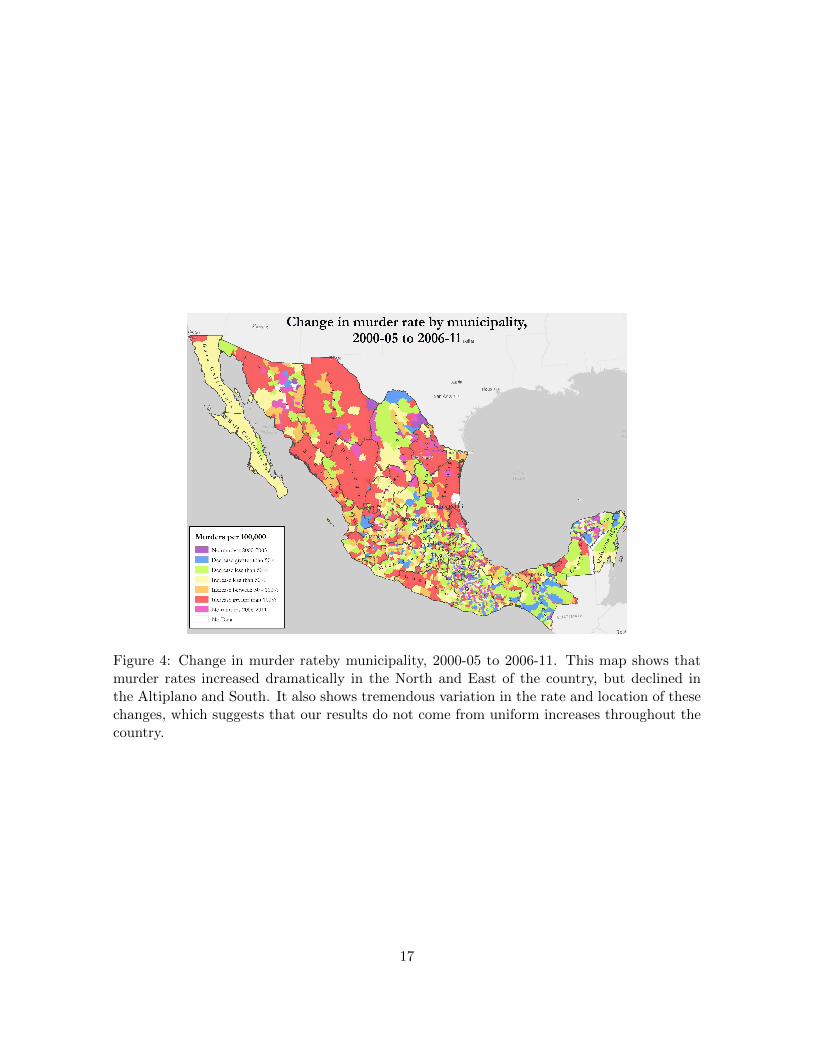
Figure 4: Change in murder rateby municipality, 2000-05 to 2006-11. This map shows thatmurder rates increased dramatically in the North and East of the country, but declined inthe Altiplano and South. It also shows tremendous variation in the rate and location of thesechanges, which suggests that our results do not come from uniform increases throughout thecountry.

17

not impose a serious constraint in our data analysis for three reasons. First, the measurement

error in our dependent variable should make it more difficult for us to find a statistically

significant relationship with our explanatory variable. Second, as non-cartel related violence

is unrelated to politics, the frequency and geographic distribution of such crime should be

relatively randomly distributed. Finally, we use several statistical techniques to control for

the unobserved mixture of cartel- and non-cartel related violence.

We code our key independent variable, Tenure, with data from the Instituto Nacional

Electoral (INE). The INE reports results at the municipal level for both legislative and general

elections.21 As voters elect new legislators every three years, we have electoral results from

the elections in 2000, 2003, 2006, and 2009. We correspondingly assigned Tenure a value of 0

in the year a district elected a political party to Congress.22 It then increases by one every

year a political party remains in office within a particular district. Should the party lose an

election, Tenure resets to 0 in the year of the election.23

Tenure is at the party, rather than individual, level due to a quirk of Mexican law. Until

electoral reforms passed in 2013, the Constitution strictly prohibited reelection in all political

offices.24 As a result, no Congressperson was reelected in the period of our study. Because

politicians cannot build personal clientelist networks and support bases, Mexican political

parties exert substantial influence over their actions. Without independent bases of support,

politicians who go against their local party officials’ wishes encounter substantial difficulty in

pursuing higher office or using their final year in office to seek alternate employment (Magaloni

2008; Mainwaring and Scully 1995; Morgenstern and Nacif 2002). As we contend that cartels

need time to learn whether it is possible to bribe political leaders, they likely work much

more closely with local political party organizations and elites than individual legislators.

Substantively, moreover, there is no variation in tenure at the individual level until 2018. For

these reasons, we code tenure based on the number of years a party — and not a politician

— remains in office.25

21We use data from Federal elections because they are complete, unlike local and state elections. To assesswhether our results hold when focusing on local elections, we reestimate our main models with data gatheredby Dell (Forthcoming) on electoral returns in some states. Those results, presented in the online appendix,suggest that the direction and significance of our measure of tenure does not change when looking at differencelevels of government.

22As is common for studies using leader tenure as a key independent variable, one concern is how to assigntransition years since there is split responsibility during that period. The appendix shows that the results arerobust (and, indeed, slightly stronger) to dropping all transition years from the analysis.

23One concern might be that some parties are more professional and therefore less likely to lose an election.However, the correlation between political party and Tenure (0.33) is not significant.

24Coming into effect in 2018, mayors may now serve two consecutive terms, while legislators may serve forup to 12 years. Once elected, they are forbidden from switching political parties.

25In a few instances, political parties campaign in coalition with a junior party. For example, the Alianzapor el Cambio was an alliance in the 2000 elections between the PAN and Green Ecological Party of Mexico.In the following election, the alliance ended and the PAN competed separately. In such cases, we do not code

18

To test the empirical implications of our formal model, we run a linear ordinary least

squares (OLS) model with municipal fixed effects and cubic restricted time splines (Green,

Kim, and Yoon 2001).26 We use municipal fixed effects to control for unit-specific factors to

reduce unobserved heterogeneity. For example, some municipalities might be more politically

competitive, have their own media market, or be located more closely to international borders.

While these are unit-specific, many such features are unobservable. We therefore include∑nj=1 θj , where θj represents a set of unobserved fixed parameters for each of the n units in

our sample. The short duration of our time series imposes certain restrictions on the number

of additional factors for which we can control. Although scholars continue to debate the

minimum number of observations per parameter necessary to avoid bias, simulations show

that the bare minimum of observations in each group per parameter is around five (Harrell

2002; Vittinghoff and McCulloch 2007). While we cannot completely eliminate the risk of

omitted variable bias and autoregressive disturbance, our results are robust to a variety of

model specifications.27

With this restriction in mind, we estimate the predicted murder level in municipality i in

year t with Equation 1:

Murderit = β0 + β1Tenureit + β2Murder(it−1) + f(γ) +

n∑j=1

θj + εit (1)

To account for the possibility of temporal dependence in our dependent variable and

autoregressive disturbances, we control for temporal effects in two ways. First, we include a

lagged dependent variable (Kiviet and Phillips 1993; Achen 2000). Second, we follow Beck,

Katz, and Tucker (1998) and include restricted cubic time splines with knots at each quartile.

A spline function is a “smoothly joined piecewise polynomial of degree n” (Durrleman and

Simon 1989, 552). Splines control for nonlinear time effects, such as the death of cartel leaders

or new smuggling routes, which affect all municipalities in the panel differently (Dickenson

2014).28 Our dependent variable Murder, is a count of the number of extralegal deaths

these party renamings as a break in incumbency.26The Nickell effect—an artificial reduction in the model’s mean square error—is a potential concern when

including fixed effects with lagged dependent variables (Nickell 1981). To explore whether this effect biases theresults presented below, we include a series of alternate specifications in our online appendix. Our results arerobust to a lagged DV without fixed effects as well as municipal- and year-fixed effects.

27As additional robustness checks, we present several alternate model specifications in the appendix. Acrossall models, including first differencing and standard OLS, Tenure remains significant and positive. It alsoremains significant and positive after controlling for whether the PRI controls a given municipality and electionyears.

28Geospatial clustering is another concern. Clustering could bias our inferences by making coefficients incon-sistent and inflating our model’s R2. To check for the presence of such clustering, we estimate a geographicallyweighted regression and present the results in the appendix. We then check for clustering in our residuals byestimating Moran’s I (Moran 1950). Results from this analysis show that our data is randomly distributed

19

recorded by the Office of the President.

3.3 Results

We report the results of our statistical model in Table 3. In line with our theoretical predic-

tions, it shows that additional years of political tenure are associated with greater violence.

This result, moreover, is robust to municipality fixed effects, cubic restricted time splines,

and a lagged dependent variable.29 While our model might appear sparse, it is worthwhile to

note that including a lagged dependent variable controls for autocorrelation and the dynamics

of the data generating process in t − 1 (Keele and Kelly 2006). Statistical research, more-

over, suggests that lagged dependent variables can suppress the coefficients of the remaining

independent variables; as such, the inclusion of a lagged dependent variable is a highly con-

servative model (Achen 2000; Durbin 1970). Together, this suggests the effect is quite robust

to alternate model specifications and is not the result of autocorrelation.

Table 2: Fixed Effects OLS of Incumbency’s Effect on Violence with Lagged DV

Dependent variable:

Murder

(1) (2)

Tenure 0.39∗∗∗ 0.16∗∗

(0.06) (0.07)

Murder−1 0.84∗∗∗ 0.84∗∗∗

(0.01) (0.01)

Municipal FE Yes YesTime Splines No YesObservations 25,538 25,538

∗p<0.1; ∗∗p<0.05; ∗∗∗p<0.01

Standard errors (clustered on municipality) reported in parentheses.

Estimates for cubic restricted time splines not reported.

To uncover the substantive effect of an additional year of tenure on murder rates, Figure 5

geospatially.29In our online appendix, we also assess whether cartels use violence strategically to influence electoral

returns. We find that the level of violence in the year of an election or the year proceeding an election has noimpact on the probability a party is returned to office, suggesting that our results are not driven by cartels’electoral manipulation.

20

2

4

6

8

10

2 4 6 8Number of Years in Power

Pre

dict

ed In

crea

se in

Mur

der T

otal

Figure 5: Estimated marginal effect for Tenure on the number of murders in a municipality.This figure shows that a one year increase in Tenure leads to an additional homicide.

plots the marginal effects of each additional year of tenure on murder rates. After setting all

other explanatory variables to their median values in Equation 1, the predicted murder rate

across all Mexican municipalities increases from 2.93 (σ = 0.87) when leaders have been in

power for only one year to 12.20 (σ = 1.80) after 11 years of tenure. This suggests that each

additional year of tenure is associated with an additional murder within a given municipality.30

While one additional murder per year might not sound substantively meaningful, it is

important to remember that this effect accrues across all 2,371 municipalities in our study.

As such, we predict that an additional 4,742 people die during the period between elections

that would not otherwise. Across the eleven years in our study, this finding suggests that

approximately 26,000 people have died in Mexico as a result of collusion between politicians

30Reverse causality — where politicians strategically deploy violence to either depress incumbents’ probabilityof reelection or frighten opposition voters away — is a potential concern with interpreting these results. Weexplore this possibility with a variety of methods in the online appendix. To summarize our findings, we findno evidence that violence affects political outcomes.

21

and cartels.

Since many political scientists are not familiar with crime statistics, it might not be clear

how to interpret an additional 2,371 deaths per year in a comparative context. As mentioned

above, according to United Nations Office of Drugs and Crime estimates, 2,371 additional

deaths per year is equivalent to the combined 2011 murder totals of France, Germany, the

United Kingdom, the Netherlands, and Belgium (UNODC 2014). While our estimate might

seem unrealistically high, Mexico is one of the world’s most violent countries. With 27,213

violent deaths reported in 2011, our estimated treatment effect only represents approximately

eight percent of all murders reported to Mexican authorities. This suggests that we can, with

relative confidence, eliminate the possibility that the effects our model has captured may be

due to modeling error.

4 Conclusion

This paper investigated a novel mechanism to explain subnational variation in violence: polit-

ical corruption. Bribery occurs because effective law enforcement hinders cartels from main-

taining territorial control and reduces their profits. Although bribes are costly, cartels want to

buy off politicians to secure their monopoly on the use of violence in their territory. Despite

cartels’ incentives to offer bribes, they are only certain to be successful when they have suffi-

cient information about officials’ corruptibility—while some politicians might be crooks, not

all are. Ultimately, increased information about politicians’ indifference points drives conflict.

To test this argument, we use data from Mexico on political tenure as a proxy for information

and show that uncertainty (as measured by time in office) is statistically and substantively

associated with lower levels of violence.

As a mechanism, political corruption has a substantively large effect on violence. In the

year following an election, we estimate that the increased information available to cartels

increases the number of homicides in Mexico by more than 2,300. This finding highlights

the clear link between politicians’ incentives and local violence. It also shows that political

institutions are important explanatory variables for both traditional civil wars as well as

violence among criminal organizations.

Beyond improving our understanding of the mechanisms that drive political violence,

we focus on the interaction between cartels and political parties because it is not trivial

for Mexican voters. Although recent reforms ended Mexico’s traditional prohibition against

reelection, this issue remains highly contentious. The threat remains that political parties

might return to their PRI-era behavior and wield significant and pernicious control over their

home regions. As our model suggests, this would lead to increased violence throughout Mexico.

22

To encourage further reform in Mexican politics, activists in Baja California launched a new

political party in 2014 aimed at ending the leadership of the two main parties and increasing

political turnover in the state. This strongly suggests that our proposed mechanism is not

far-fetched to Mexican voters.

Our results have important implications for future study of the relationship between po-

litical institutions and conflict. First, scholars commonly assume that ideology determines

a violent group’s choice to fight the state or attempt to co-opt it (McAdam, et al. 2003).

Instead, both our model and empirical results suggest that this decision might instead be

conditional upon the group’s access to rents. Rich groups should find it easier to bribe and

co-opt officials. In contrast, poor groups might not have access to sufficient resources to make

bribery a viable option. Second, electoral laws that favor status quo parties—such as min-

imum vote thresholds and public financial support for parties—might have the unintended

consequence of improving violent groups’ odds at bribing officials. Practically, this implies

that lobbying against such laws might help activist groups improve domestic security.31 Fi-

nally, and perhaps most troublingly, our results show that there is no easy fix to the cartel

problems in Mexico.

Our paper’s implications also raise questions about when strengthening democratic insti-

tutions reduces violence. The civil war literature suggests that making politicians accountable

to voters through competitive elections should decrease rent-seeking behavior and their toler-

ance for violence. This strategy was successful in decreasing cartel violence during Prohibition

in the United States and among Mafia in Italy yet has largely failed in Latin America (Varese

2011). We help explain this variation by demonstrating that elections are only one mech-

anism that explains a state’s monopoly on violence. Future research might investigate the

effect of specific institutions, such as independent anti-corruption investigators. By investi-

gating politicians who accept bribes, such institutions plausibly make it too risky to cooperate

with violent agents. These institutions, rather than elections, might be key to reducing cartel

violence.

Finally, the scope of our project is limited to understanding how cartels and local officials

conspire with each other for mutual benefit at the expense of rival cartels and the municipal-

ity’s citizens. However, this is only one interesting strategic aspect of the Mexican drug wars.

Future research ought to consider how cartels negotiate with each other and how national

intervention in local affairs complicates the larger bargaining and enforcement process.

31Of course, implementing such reforms might require herculean effort—those in power have strong incentivesto maintain and strengthen the systems that put them in office. Moreover, artificially reducing party tenurecould have unintended negative consequences, as experience and professionalization are desirable in other policyareas.

23

5 Appendix: Formal Proofs

5.1 Proof of Proposition 1

We proceed with backward induction. Fix a level of enforcement α. Cartel 1’s objective

function is v1v1+v2

− αv1, with its choice a value for v1. Its first order condition is therefore:

v2(v1 + v2)2

− α = 0 (2)

Meanwhile, Cartel 2’s objective function is 1 − v1v1+v2

− v2, with its choice a value for v2.

Its first order condition is therefore:

v1(v1 + v2)2

− 1 = 0 (3)

Using Equations 2 and 3 as a system of equations, the unique solution pair is v∗1 =1

(1+α)2, v∗2 = α

(1+α)2. Note that when the politician accepts the bribe, α = α and therefore the

solution pair is v∗1 = 1(1+α)2

, v∗2 = α(1+α)2

.32

Now consider the party’s enforcement level, conditional on its rejection of the bribe. The

party’s objective function is−(v1+v2)−k(α), with its choice a value for α. Because v∗1 = 1(1+α)2

and v∗2 = α(1+α)2

, we can rewrite this as − 11+α − k(α). The first portion is strictly concave,

while the second is weakly concave. Therefore, the addition of the two is strictly concave.

This implies that the objective function has a unique solution. Call that solution α∗.

The remaining task is to solve for the bargaining game. We first look at the politician’s

accept or reject decision. Accepting yields −(v∗1 + v∗2) + bc. Substituting for the equilibrium

levels of violence, we have:

− 1

(1 + α)+ bc (4)

Meanwhile, the politician receives −(v∗1 + v∗2)− k(α∗) if it rejects. Again substituting for

the equilibrium levels of violence, we have:

− 1

(1 + α∗)− k(α∗) (5)

Using Equations 4 and 5, the politician is willing to accept any a bribe if:

32Note that the objective functions are undefined for v1 = v2 = 0. Regardless of the rule we use to defineeach objective function’s value in that instance, v1 = v2 = 0 cannot be part of any equilibrium—as is standardfor contest success functions, the marginal value for investing a slight amount overwhelms the cost to do soand is therefore a profitable deviation for at least one player.

24

− 1

(1 + α)+ bc ≥ − 1

(1 + α∗)− k(α∗)

b ≥ b ≡1

1+α −1

1+α∗ − k(α∗)

c(6)

That leaves Cartel 1’s bribe decision. To analyze this, we first need to find 1’s payoffs in

the violence decision subgames with and without enforcement. Without enforcement, recall

that the equilibrium levels of violence are v∗1 = 1(1+α)2

, v∗2 = α(1+α)2

. Plugging these into Cartel

1’s utility function gives:

1

(1 + α)2(7)

In contrast, with enforcement, the equilibrium levels of violence are v∗1 = 1(1+α∗)2 , v

∗2 =

α∗

(1+α∗)2 . Thus, Cartel 1’s utility function for an unsuccessful bribe is:

1

(1 + α∗)2(8)

Combining Equations 7 and 8, Cartel 1’s utility differential between successful and unsuc-

cessful negotiations equals:

b ≡ 1

(1 + α)2− 1

(1 + α∗)2(9)

This is also the maximum bribe Cartel 1 is willing to pay. Using Equations 6 and 9 as the

constraints, a mutually acceptable bargain exists if:

b < b

c > c∗ ≡1

(1+α)2− 1

(1+α∗)2 − k(α∗)

1(1+α)2

− 1(1+α∗)2

So if c > c∗, Cartel 1 offers the politician’s minimally acceptable amount (b), and the

politician accepts. If c < c∗, no bribe is mutually acceptable. Cartel 1 is then free to offer any

bribe less than b, guaranteeing the politician’s rejection. Note that Proposition 2 therefore

applies to all cases where c′ < c∗.

5.2 Proof of Proposition 3 and 4

To begin, let b′ =1

1+α− 1

1+α∗−k(α∗)

c′ and b′′ =1

1+α− 1

1+α∗−k(α∗)

c . These values represent the

minimally acceptable bribe to the more corrupt and the less corrupt types. Note that b′′ > b′,

25

so it costs more to bribe the less corrupt type.

No equilibria exist in which Cartel 1 offers a value not equal to b′′ or b′. To see why,

consider proof by cases. If Cartel 1 offers b > b′′, both types accept. Cartel 1 receives 1(1+α)2

for the remainder of the game. However, Cartel 1 could alternatively offer the midpoint

between that offered bribe and b′′. Because that value is still strictly greater than b′′, both

types still accept. Cartel 1 in turn receives 1(1+α)2

. But note that it receives this same payoff

but pays a strictly smaller bribe. This is a profitable deviation. Therefore, offering b > b′′ is

never optimal.

Next, offering b < b′ is not optimal either. Such an offer induces both types to reject.

Cartel 1’s payoff therefore equals 1(1+α∗)2 . In contrast, consider an offer b ∈ (b′, b′′) instead.

That amount induces the more corrupt type to accept and the less corrupt type to reject. In

turn, Cartel 1’s payoff is equivalent if it is facing the less corrupt type. However, with positive

probability, it is facing the more corrupt type. Because that offer is in the bargaining range

for the more corrupt type, Cartel 1 earns strictly more than in this case than if bargaining

fails. This is a profitable deviation. Therefore, offering b < b′ is not optimal.

Finally, consider b ∈ (b′, b′′). As discussed above, such an offer induces the more corrupt

type to accept and the less corrupt type to reject. Now consider a deviation to the midpoint

between that offer and b′. This amount is still strictly greater than b′ and strictly less than

b′′. Consequently, the more corrupt type still accepts and the less corrupt type still rejects.

Cartel 1’s payoff for the contest portion of the game remains the same. However, it pays a

strictly smaller bribe to the more corrupt type. This is a profitable deviation. Therefore,

offering b ∈ (b′, b′′) is not optimal.

That information means that strategies can only satisfy equilibrium conditions if Cartel 1

offers b′ or b′′. In the first case, note that the weak type is indifferent between accepting and

rejecting; in the second case, the strong type is indifferent. For reasons standard to ultimatum

games like this one, no equilibria exist when one of those types rejects with positive probability

when indifferent. This leaves two possibilities: Cartel 1 offers b′′ and both types accept with

certainty and Cartel 1 offers b′, the more corrupt type accepts with certainty, and the less

corrupt type rejects.

To see which offer prevails under equilibrium conditions, note that offering b′′ yields Cartel

1 a flat payoff of 1(1+α)2

− b′′. Offering b′ leads to a probabilistic outcome: Cartel 1 receives1

(1+α)2− b′ with probability p and 1

(1+α∗)2 with probability 1 − p. As such, making the safe

offer is optimal if:

1

(1 + α)2− b′′ > p

(1

(1 + α)2− b′

)+ (1− p)

(1

(1 + α∗)2

)

26

p < p∗ ≡1

(1+α)2− 1

(1+α∗)2 − b′′

1(1+α)2

− 1(1+α∗)2 − b′

(10)

By analogous argument, Cartel 1 offers b′ if p > p∗.

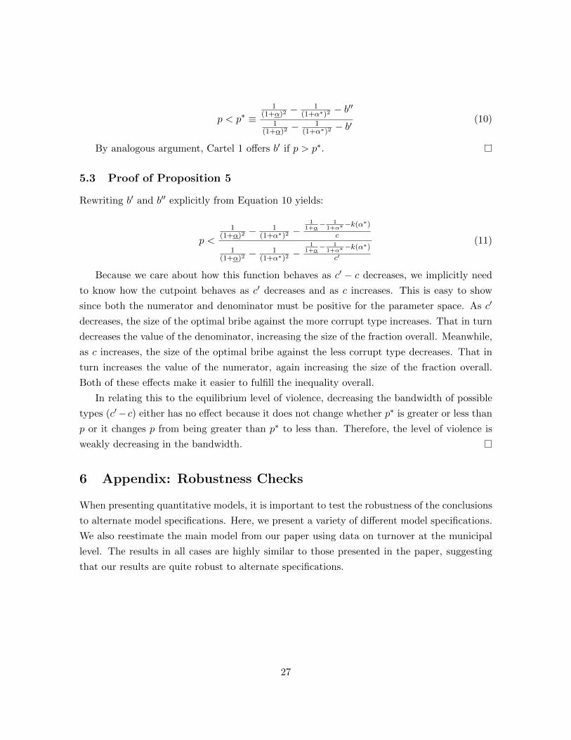
5.3 Proof of Proposition 5

Rewriting b′ and b′′ explicitly from Equation 10 yields:

p <

1(1+α)2

− 1(1+α∗)2 −

11+α− 1

1+α∗−k(α∗)

c

1(1+α)2

− 1(1+α∗)2 −

11+α− 1

1+α∗−k(α∗)c′

(11)

Because we care about how this function behaves as c′ − c decreases, we implicitly need

to know how the cutpoint behaves as c′ decreases and as c increases. This is easy to show

since both the numerator and denominator must be positive for the parameter space. As c′

decreases, the size of the optimal bribe against the more corrupt type increases. That in turn

decreases the value of the denominator, increasing the size of the fraction overall. Meanwhile,

as c increases, the size of the optimal bribe against the less corrupt type decreases. That in

turn increases the value of the numerator, again increasing the size of the fraction overall.

Both of these effects make it easier to fulfill the inequality overall.

In relating this to the equilibrium level of violence, decreasing the bandwidth of possible

types (c′− c) either has no effect because it does not change whether p∗ is greater or less than

p or it changes p from being greater than p∗ to less than. Therefore, the level of violence is

weakly decreasing in the bandwidth.

6 Appendix: Robustness Checks

When presenting quantitative models, it is important to test the robustness of the conclusions

to alternate model specifications. Here, we present a variety of different model specifications.

We also reestimate the main model from our paper using data on turnover at the municipal

level. The results in all cases are highly similar to those presented in the paper, suggesting

that our results are quite robust to alternate specifications.

27

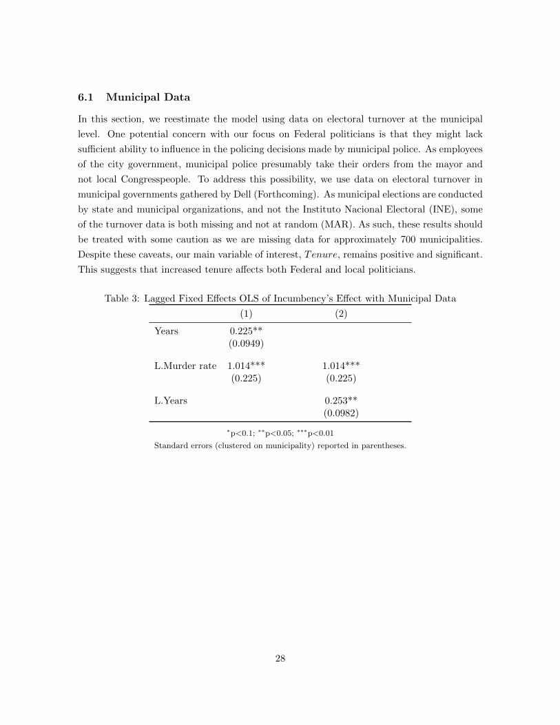
6.1 Municipal Data

In this section, we reestimate the model using data on electoral turnover at the municipal

level. One potential concern with our focus on Federal politicians is that they might lack

sufficient ability to influence in the policing decisions made by municipal police. As employees

of the city government, municipal police presumably take their orders from the mayor and

not local Congresspeople. To address this possibility, we use data on electoral turnover in

municipal governments gathered by Dell (Forthcoming). As municipal elections are conducted

by state and municipal organizations, and not the Instituto Nacional Electoral (INE), some

of the turnover data is both missing and not at random (MAR). As such, these results should

be treated with some caution as we are missing data for approximately 700 municipalities.

Despite these caveats, our main variable of interest, Tenure, remains positive and significant.

This suggests that increased tenure affects both Federal and local politicians.

Table 3: Lagged Fixed Effects OLS of Incumbency’s Effect with Municipal Data

(1) (2)

Years 0.225**(0.0949)

L.Murder rate 1.014*** 1.014***(0.225) (0.225)

L.Years 0.253**(0.0982)

∗p<0.1; ∗∗p<0.05; ∗∗∗p<0.01

Standard errors (clustered on municipality) reported in parentheses.

28

6.2 Reverse Causality

One potential concern with interpreting the above results is reverse causality. Cartels might

strategically use violence ahead of elections to scare the public away from polls; politicians

could target incumbents by increasing violence to make them appear weaker; or politicians

could use violence against opposition voters. This might bias our results by inflating the

relationship between political tenure and murder, yet provide no support for the mechanism

we model in this paper because the violence results from political competition rather than

cartels. To explore whether a municipality’s murder rate affects the probability the incumbent

political party is reelected, we include a variable Reelection that takes a value of 1 in years

when a political party is elected to office (and zero otherwise). If the above concern about

reverse causality were correct, we should observe that violence should be correlated with

reelection (either positively or negatively). Using a panel model probit with time splines, we

find no relationship between murder and the probability of reelection. This strongly suggests

that pre-electoral violence does not drive our results.

Table 4: Probit of Murder’s Effect on Probability of Reelection

Dependent variable:

Reelection(1) (2) (3)

Murder Rate -0.00 -0.00(0.00) (0.000)

L.Murder Rate -0.00(0.00)

Time Splines No Yes Yes∗p<0.1; ∗∗p<0.05; ∗∗∗p<0.01

Standard errors reported in parentheses.

29

6.3 Lagged Independent Variable

One concern with our results is that they might be driven by reverse causality, i.e. a party’s

electoral fate is decided by the current level of violence. This would introduce simultaneity

bias wherein an unobserved variable that explains both levels of violence and electoral success

biases the error term in our results. One common way to address this issue is through

an instrumental variable, where an exogenous variable is used to perform a two-stage OLS.

Unfortunately, we are unable to identify a good instrument that predicts which parties are

reelected and is also satisfies the exclusion restriction that it is uncorrelated with violence. To

address this potential problem, we follow Clemens, et al. (2012, 1) and “avoid poor quality

instrumental variables and instead address potential biases from reverse and simultaneous

causation by the more transparent methods of lagging and differencing.” This is a relatively

common econometric technique to overcome simultaneity bias. We then estimate the predicted

murder level in municipality i in year t with Equation 12:

∆Murderit = ∆β0 + β1∆Tenureit−1 + β2∆Murderit−1 + ∆f(γ) + ∆εit (12)

The results from this model are presented in Table 5:

Table 5: Lagged Fixed Effects OLS of Incumbency’s Effect on Violence with First Differences

Dependent variable:

Murder

(1) (2)

LD.Congress Tenure 0.27*** 0.29***(0.05) (0.05)

LD.Murder Rate 1.48*** 1.48***(0.14) (0.14)

District FE Yes YesTime Splines No YesObservations 25,517 25,517

∗p<0.1; ∗∗p<0.05; ∗∗∗p<0.01

Standard errors (clustered on municipality) reported in parentheses.

Estimates for cubic restricted time splines not reported.

As these results show, the finding presented in the body of the paper likely does not result

from simultaneity bias and is robust to a lagged IV.

30

6.4 Lagged DV with Fixed Effects

The Nickell effect is a concern when including fixed effects in a lagged dependent variable

model. By including fixed effects, one might bias results by artificially deflating the model’s

mean square error (MSE). This is particularly problematic with a small number of time

periods in the data. Beck and Katz (2009) show that the bias produced by the Nickell effect

is less than some of the proposed solutions, such as the Kiviet method. As such, this suggests

that the results presented in the body of the paper are one modeling choice with TCSC data.

It is still possible, however, that our results remain biased by the Nickell effect. To explore

this possibility, we first reestimate our model with a lagged dependent variable without fixed

effects. Second, we reestimate our results with year- and municipal-fixed effects. The results

from these models are presented in Table 6:

Table 6: Lagged DV Without FE and Year FE

Dependent variable:

Murder

(1) (2)

Congress Tenure 0.22*** 0.47**(0.05) (0.23)

L.Murder Rate 0.99*** -(0.05) -

Municipal FE No YesYear FE No Yes

∗p<0.1; ∗∗p<0.05; ∗∗∗p<0.01

Bootstrapped errors reported in parentheses.

Estimates for year fixed effects not reported.

As Table 6 shows, our results remain broadly consistent (and in fact the coefficient on

Congress Tenure becomes larger) without municipal FE. This suggests that the results re-

ported in the main body of the paper are not strongly biased by the Nickell effect. Second, we

show that our choice to model time with splines is not necessary to obtain our results. After

using year fixed effects, our variable of interest continues to have a positive and statistically

significant effect on violence.

31

6.5 First Differences

Our first robustness check is a first differences time series pooled ordinary least squares (OLS)

regression. Unlike standard OLS, a first difference model subtracts the observed values of the

dependent and independent variables in t = 1 from t = 2. In the process of subtracting,

taking the first difference removes all invariant, unit-specific factors, denoted by θ.33 This is

because all of the factors contained within θ do not change between time periods, meaning

they reduce to zero.

We estimate the predicted murder level in municipality i in year t with Equation 13:

∆Murderit = ∆β0 + β1∆Tenureit + ∆f(γ) + ∆εit (13)

The results from this model are presented in Table 7:

Table 7: Fixed Effects OLS of Incumbency’s Effect on Violence with First Differences

Dependent variable:

Murder

(1) (2)

D.Congress Tenure 0.05** 0.05**(0.03) (0.03)

District FE Yes YesTime Splines No YesObservations 25,517 25,517

∗p<0.1; ∗∗p<0.05; ∗∗∗p<0.01

Standard errors (clustered on municipality) reported in parentheses.

Estimates for cubic restricted time splines not reported.

33First differences are not the only estimation technique to control for unobserved heterogeneity. Manyscholars use fixed effects to do so. Although we present results using district fixed effects in the online appendix,we believe fixed effects’ assumption that the error term is serially independent to be harder to justify. Murderrates in t = 0 likely are likely highly predictive of violence in t = 1. As serial correlation incorrectly decreasesthe coefficients’ standard errors, this is a serious specification issue. First differences, in contrast, are morerobust to violations of this assumption (Liker, et al. 1985).

32

6.6 Fixed Effects OLS

In this section, we estimate use the following equation to estimate a fixed effects OLS regres-

sion:

Murderit = β0 + β1Tenureit + f(γ) +n∑j=1

θj + εit (14)

The results, presented in the table below, are also statistically significant and in the right

direction.

Table 8: Fixed Effects OLS of Incumbency’s Effect on Violence

Dependent variable:

Murder

(1) (2) (3)

Tenure 0.84∗∗∗ 0.47∗∗∗ 0.26∗∗

(0.07) (0.11) (0.11)

PRI 4.21∗∗∗

(0.68)

ElectionYear 0.93∗∗

(0.41)

Observations 27,861 27,861 27,861Municipal FE Yes Yes YesTime Splines No Yes Yes

∗p<0.1; ∗∗p<0.05; ∗∗∗p<0.01

Standard errors (clustered on municipality) reported in parentheses.

Estimates for cubic restricted time splines not reported.

33

6.7 Coding of Independent Variable

In the main body of the paper, we code our main independent variable — Tenure— as linearly

increasing year-on-year. One concern with this might be that each additional year a political

party remains in office might not in fact provide substantial additional information to cartels.

Instead, cartels might update only after each election and then adopt similar bargaining

strategies with politicians during their time in office. To address this possibility, we recode

Tenure so that it increases only when a political party secures reelection. This reduces the

scale of our new Tenure∗ variable from 11 to 4 (σ = 0.95, µ =1.83). We then estimate

the effect of an increase in this Tenure variable with a cross sectional Poisson regression.

As before, increases in Tenure are positively and significantly associated with an increased

number of homicides in a given municipality.

Table 9: Recoding Key Independent Variable

Dependent variable:

Murder

(1) (2)

Tenure∗ 0.06∗∗∗ 0.06∗∗∗

(0.01) (0.01)

L.Murder 0.00∗∗∗ 0.00∗∗∗

(0.00) (0.00)

Observations 25,943 24,629Municipal FE No YesTime Splines Yes Yes

∗p<0.1; ∗∗p<0.05; ∗∗∗p<0.01

Standard errors (clustered on municipality) reported in parentheses.

Estimates for cubic restricted time splines not reported.

34

6.8 Count Data

Our dependent variable, the number of homicides a municipality experiences in a year, cannot

take negative values. As such, it is an example of count data. While OLS estimators are

BLUE for count data, they could potentially be inefficient. Correcting for this inefficiency

might affect estimated coefficient direction, significance, or show that the model does not

appropriately fit the data. To address this possibility, we present the results here from a class

of models specifically designed for count data — a cross sectional Poisson regression. These

results, presented in Table ??, show that our main coefficient of interest is not affected by

accounting for count data.

Table 10: Poisson Regression

Dependent variable:

Murder

(1) (2)

Tenure 0.03∗∗∗ 0.03∗∗∗

(0.002) (0.002)

L.Murder 0.00∗∗∗ 0.00∗∗∗

(0.00) (0.00)

Observations 25,538 24.224Municipal FE No YesTime Splines Yes Yes

∗p<0.1; ∗∗p<0.05; ∗∗∗p<0.01

Standard errors (clustered on municipality) reported in parentheses.

Estimates for cubic restricted time splines not reported.

35

6.9 Power Transition Years

Empirical models that use tenure as a key independent variable inevitably face problems

coding transition periods. With elections midway through the election year, it is difficult for

the researcher to know exactly whom to assign the murders to. In the interest of completeness,

the main model included the transition years. However, there are two relevant alternative

coding schemes. The first assigns all the murders to the party in power at the beginning

of the year. Some may find this coding scheme preferable because fresh leaders may not

have held office long enough to sway policy in a meaningful way. Running the main model

specification with the alternative coding scheme generates the following results:

Table 11: Fixed Effects OLS with Lagged DV Subsetting Transition Years

Dependent variable:

Murder

(1) (2)

Tenure 0.17∗∗ 0.17∗∗

(0.07) (0.07)

Murder−1 0.84∗∗∗ 0.84∗∗∗

(0.01) (0.01)

Observations 25,517 25,517

∗p<0.1; ∗∗p<0.05; ∗∗∗p<0.01

Standard errors (clustered on municipality) reported in parentheses.

Estimates for cubic restricted time splines not reported.

As Table 11 shows, our Tenure variable remains positive and significant with this alternate

specification.

The second alternative scheme is the most conservative option available. It removes all

transition years from the data. In other words, if a party does not hold office for the entire

year, we subset it out of the analysis. Note that this is not the same as removing all election

years—for elections where the incumbent party wins, we know who is responsible for the

murders in that year.

As Table 12 illustrates, the model is robust to this specification. Moreover, the effect is

stronger here. While it is important not to overanalyze these differences, we would expect this

to be true given our mechanism. After all, if transition years mix the “correct” assignment of

homicides, the model would systematically underreport the actual effect due to newer leaders

36

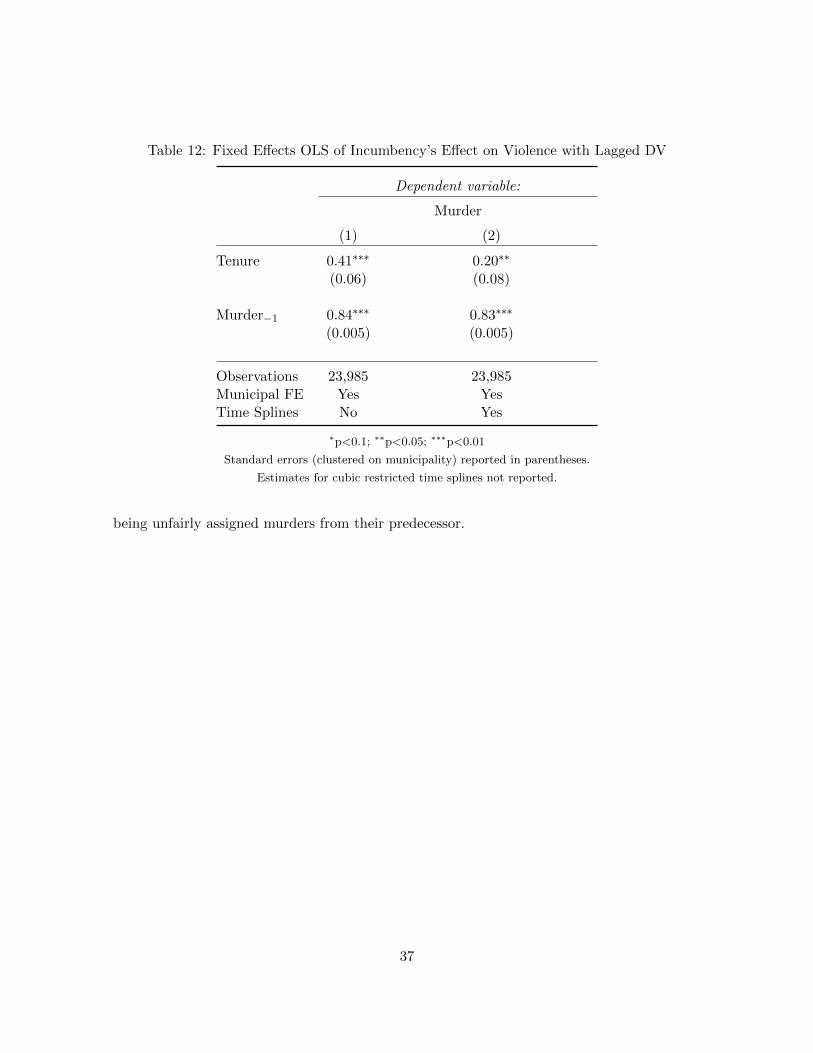
Table 12: Fixed Effects OLS of Incumbency’s Effect on Violence with Lagged DV

Dependent variable:

Murder

(1) (2)

Tenure 0.41∗∗∗ 0.20∗∗

(0.06) (0.08)

Murder−1 0.84∗∗∗ 0.83∗∗∗

(0.005) (0.005)

Observations 23,985 23,985Municipal FE Yes YesTime Splines No Yes

∗p<0.1; ∗∗p<0.05; ∗∗∗p<0.01

Standard errors (clustered on municipality) reported in parentheses.

Estimates for cubic restricted time splines not reported.

being unfairly assigned murders from their predecessor.

37

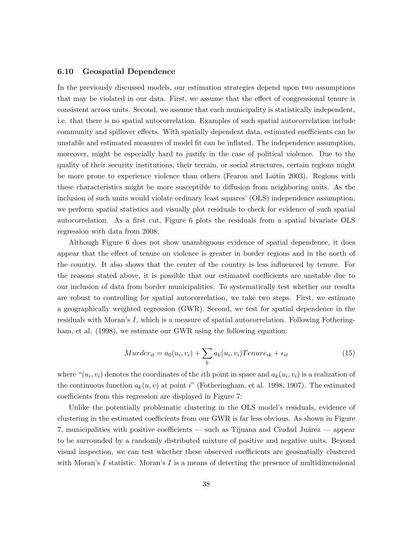
6.10 Geospatial Dependence

In the previously discussed models, our estimation strategies depend upon two assumptions

that may be violated in our data. First, we assume that the effect of congressional tenure is

consistent across units. Second, we assume that each municipality is statistically independent,

i.e. that there is no spatial autocorrelation. Examples of such spatial autocorrelation include

community and spillover effects. With spatially dependent data, estimated coefficients can be

unstable and estimated measures of model fit can be inflated. The independence assumption,

moreover, might be especially hard to justify in the case of political violence. Due to the

quality of their security institutions, their terrain, or social structures, certain regions might

be more prone to experience violence than others (Fearon and Laitin 2003). Regions with

these characteristics might be more susceptible to diffusion from neighboring units. As the

inclusion of such units would violate ordinary least squares’ (OLS) independence assumption,

we perform spatial statistics and visually plot residuals to check for evidence of such spatial

autocorrelation. As a first cut, Figure 6 plots the residuals from a spatial bivariate OLS

regression with data from 2008:

Although Figure 6 does not show unambiguous evidence of spatial dependence, it does

appear that the effect of tenure on violence is greater in border regions and in the north of

the country. It also shows that the center of the country is less influenced by tenure. For

the reasons stated above, it is possible that our estimated coefficients are unstable due to

our inclusion of data from border municipalities. To systematically test whether our results

are robust to controlling for spatial autocorrelation, we take two steps. First, we estimate

a geographically weighted regression (GWR). Second, we test for spatial dependence in the

residuals with Moran’s I, which is a measure of spatial autocorrelation. Following Fothering-

ham, et al. (1998), we estimate our GWR using the following equation:

Murderit = a0(ui, vi) +∑k

ak(ui, vi)Tenureik + εit (15)

where “(ui, vi) denotes the coordinates of the ith point in space and ak(ui, vi) is a realization of

the continuous function ak(u, v) at point i” (Fotheringham, et al. 1998, 1907). The estimated

coefficients from this regression are displayed in Figure 7:

Unlike the potentially problematic clustering in the OLS model’s residuals, evidence of

clustering in the estimated coefficients from our GWR is far less obvious. As shown in Figure

7, municipalities with positive coefficients — such as Tijuana and Ciudad Juarez — appear

to be surrounded by a randomly distributed mixture of positive and negative units. Beyond

visual inspection, we can test whether these observed coefficients are geosnatially clustered

with Moran’s I statistic. Moran’s I is a means of detecting the presence of multidimensional

38

Figure 6: OLS residuals by municipality for 2008. Note that Oaxacan municipalities do notfollow a consistent naming pattern and are excluded from this analysis.

39

Figure 7: Coefficient estimated by GWR for all municipalities in 2008. Note that Oaxacanmunicipalities do not follow a consistent naming pattern and are excluded from this analysis.

40

correlation in geospatial data (Paradis 2014). Moran’s I, as defined by Moran (1950) is:

I =N∑

i=1

∑j=1

wij

∑i=1

∑j=1

wij(Xi − X)(Xj − X)∑i=1

(Xi − X)2(16)

where N is the number of units in the sample; X is our variable of interest (in this case,

Tenure), X is the mean of X; and wij is an index of spatial weights. As the null hypothesis

is no spatial autocorrelation, the expected value of I0 is defined as I0 = −1/n − 1). The

expected value of 10 is known, we can test for a statistically significant difference between

the observed I (I) and I0. When I0 > I, it suggests evidence of positive spatial correlation.

In contrast, when 10 < I, it is evidence of negative spatial correlation. Finally, when I0 is

not statistically distinguishable from I, we cannot reject the null hypothesis that the data is

randomly distributed spatially (Paradis 2014).

In this case, we use Equation 16 to estimate the Moran’s I for our model. Our estimated I

— i.e. I —is 0.002. We then test whether this estimated value is statistically distinguishable

from the expected value of I under the null hypothesis, which is -0.0005. The p-value of the

difference between these two values is 0.20, which means we cannot reject the null hypothesis.

Although this does not definitely prove that there is no spatial dependence, it strongly suggests

that there is no statistical evidence for it that is discernible in our data.

41