Geostatistics without Stationarity Assumptions within GIS

Alexander Brenning∗ K. Gerald van den Boogaart†

Abstract

The present work deals with two challenging problems of applied geostatistics: (i) Station-arity assumptions often do not hold under real-world conditions. (ii) Geostatistical methodshave to be linked with spatial databases in order to be applicable in non-stationary situations.Solutions for both problems are proposed and implemented.

(i) A central assumption in geostatistics is the stationarity of the process. However thespatial variability of many natural phenomena heavily depends on the local geology, which isnon-stationary in most cases. To deal with this, the concept of process stationarity is replaced bya stationarity of the governing influence relating the local semivariogram and the local geology asstored in a Geographical Information System (GIS). A construction method is used, which canmeaningfully incorporate additional spatial information from GIS, e.g. smoothly varying geologyin the investigated area or geological faults interrupting continuity. Least-squares parameterestimation is used for fitting instationary semivariogram models in typical example situations,leading to non-linear optimization problems.

(ii) Geostatistical tools that make use of the local geology need direct access to the data storedin the GIS. A link between the presented geostatistical tools and the GIS software ArcView wasestablished. Thus, spatial data such as soil properties and morphology can be incorporated ingeostatistical analyses.

R code that fits instationary semivariogram models and performs kriging is provided. It isapplied to simulated data.

Resumen

Este trabajo trata dos problemas desafiantes de la geoestadıstica aplicada: (i) Bajo condi-ciones reales, muchas veces no son validas las suposiciones de estacionaridad. (ii) Los metodosgeoestadısticos deben ser vinculados con bases de datos espaciales para ser aplicables en situa-ciones no estacionarias. Se proponen e implementan soluciones para ambos problemas.

(i) En geoestadıstica, una suposicion central es la estacionaridad del proceso. Sin embargo,la variabilidad espacial de muchos procesos depende estrechamente de la geologıa local, la cuales inestacionaria en la mayorıa de los casos. Para tratar esto, el concepto de estacionaridad delproceso es reemplazado por una estacionaridad de una ley de influencia; esta vincula el semi-variograma con la geologıa local tal como esta guardada dentro de un Sistema de InformacionGeografico. Se usa un metodo de construccion que permite incorporar informacion espacial deun SIG, por ejemplo una geologıa que varıa de manera contınua dentro del area de estudio o fal-las geologicas que interrumpen la continuidad. Se aplica una estimacion de mınimos cuadradospara ajustar modelos parametricos de semivariogramas inestacionarios en situaciones ejemplarestıpicas, resultando en problemas de optimizacion no lineales.

(ii) Herramientas geoestadısticas que se apoyan en la geologıa local precisan de un accesodirecto a los datos guardados en el SIG. Se establecio un vınculo entre la herramienta geoes-tadıstica presentada y el SIG ArcView. De esta manera pueden incorporarse a los analisisgeoestadısticos datos espaciales tales como propiedades del suelo y la morfologıa.

Se facilita un codigo de R que ajusta modelos de semivariogramas inestacionarios y realizakrigeado. El codigo es aplicado a datos simulados.

∗Friedrich-Alexander-Universitat Erlangen–Nurnberg, Institut fur Geographie, Kochstr. 4/4, 91054 Erlangen, Ger-many, e-mail ali@proforma.de.†TU Freiberg, Institut fur Geologie, B.-v.-Cotta-Str. 2, 09596 Freiberg, Germany, e-mail boogaart@iname.com.

1

1 Introduction

The amount of spatial information that is available within GIS is increasing rapidly due to the col-lection of thematic data using remote sensing techniques. These data are often useful for modelinglocal (non-geometrical) anisotropies following morphology or tectonic structures, e. g. This devel-opment creates a need for instationary geostatistical methods that meaningfully incorporate thisinformation, enabling us to model complex geologic situations such as tectonic faults interruptingcontinuity or drainage systems inducing nested patterns of anisotropy. These methods must belinked with a GIS.

2 Theoretical Background

We consider a real-valued stochastic processes Z = (Zs)s∈D of second order with parameter setD ⊂ Rd, d ≥ 2.

2.1 A Method of Instationary Covariogram Construction

We study processes with covariograms that are induced by a weight function. We will see that theseinduced covariograms approximate stationary covariograms arbitrarily well. Of particular interestwill be weight functions that incorporate covariables describing local conditions such as anisotropy.Let E be a non-empty measurable Borel set in Rd.

Definition 2.1 A weight function on D×E is an arbitrary function w : D×E → R such that forall s ∈ D

νw(s) :=∫Ew(s, p)2 dp <∞.

A weight function on D × E is called isotropic, if there exists a function wi : R → R such thatw(s, p) = wi(‖p− s‖) for all s ∈ D, p ∈ E.

Theorem 2.2 For an arbitrary weight function w on D×E and all s, t ∈ D there exists the integral

Cw(s, t) :=∫Ew(s, p)w(t, p) dp, (1)

and the function Cw is positive semidefinite. Furthermore, Cw is the covariogram of a second-orderprocess on D; it is called the covariogram induced by w.

Proof: The integral in (1) exists and is finite. Furthermore, if for n ∈ N, we choose arbitraryt1, . . . , tn ∈ and a1, . . . , an ∈ R, then we obtain

n∑i=1

n∑j=1

aiajCw(ti, tj) =n∑i=1

n∑j=1

aiaj

∫Ew(ti, p)w(tj , p) dp

=∫E

n∑i=1

aiw(ti, p)n∑j=1

w(tj , p) dp =∫E

(n∑i=1

aiw(ti, p)

)2

dp ≥ 0.

Hence Cw is positive semidefinite. Cw is also symmetric, so there exists a second-order process onD with covariogram Cw. 2

Remark 2.3 The semivariogram γ corresponding to a covariogram C that is induced by an arbi-trary weight function w is of the form

γ(s, t) = 12C(s, s) + 1

2C(t, t)− C(s, t)

= 12

∫Rd

(w(s, p)2 + w(t, p)2 − 2w(s, p)w(t, p)

)dp

= 12

∫Rd

(w(s, p)− w(t, p))2 dp. (2)

2

Theorem 2.4 (Approximation of stationary covariograms) Every stationary covariogram Con Rd that has a spectral density g = dG/dλ can be approximated arbitrarily well with respect tothe essential supremum ‖ · ‖∞ by an induced covariogram, i. e.: For every ε > 0 there exists atranslation invariant weight function w(s, t) = ws(t− s) that induces a covariogram Cw with

‖C − Cw‖∞ < ε.

Proof: Cf. van den Boogaart (1999).

Remark 2.5 Assuming the existence of a spectral density in Theorem 2.4 implies that neither anugget effect nor a covariogram not vanishing as ‖h‖ → ∞ can be approximated arbitrarily well byweight functions. However a nugget effect can be added a posteriori to an induced covariogram.

For motivation we now present a well-known example of an induced covariogram that is isotropic(cf. Wackernagel (1998)). Later it will be used as a point of departure for modeling anisotropies.

Example 2.6 (Spherical covariograms) For fixed a = 2R > 0 and E = Rd ⊃ D, consider theisotropic weight function

w : D ×Rd → R, w(s, p) = 1[0,R)(‖p− s‖), s ∈ D, p ∈ Rd.

and its normalization scaled by σ > 0,

w(s, p) = σ · w(s, p)/√νw(s) = σ · 1[0,R)(‖p− s‖)/λd(Bd(0, R)).

We study the covariograms induced by w for d = 3, 2, which writes

Cw(s, t) = σ2 · λd(Bd(s,R) ∩Bd(t, R)

)/ λd(0, R).

i) d = 3: We get the spherical covariogram in three dimensions. The usual two-dimensional versionis obtained by taking D′ = D × 0, D ⊂ R2.ii) d = 2: We have to calculate the area of dissection of two discs of radius R in R2. Geometricalconsiderations yield

Cw(h) = σ2

π

(2 arccos (h/a)− h

4a2

√a2 − h2

), if h < a,

0 otherwise. The isotropic covariogram Cw is continuous, but its first derivative has a singularityat h = 2R, unlike the spherical covariogram.

2.2 Modeling Local Anisotropy

Theorem 2.4 showed that the class of covariograms induced by a weight function is sufficiently largeas to be useful instruments for covariogram modeling. The construction method will be used forcreating a class of semivariograms and covariograms that can adapt to local anisotropies that maybe quite irregular, but follow a known pattern.From now on we choose d = 2 and E ⊂ R2.

Definition 2.7 (Elliptical covariograms) Let woτ : R → R, τ ∈ T 6= ∅, be an isotropic weightfunction with support ⊂ B2(0, 1). For r ≥ 0, q ∈ (0, 1] and φ ∈ [0, π) we define

R(r, q, φ) =1r

(cosφ sinφ

−q−1 sinφ q−1 cosφ

)to be a combined contraction and rotation by −φ satisfying

R(r, q, φ)Ell(0; r, q, φ) = B2(0, 1),

3

0

sill a) b)

0 range

0

sill c)

0 range

d)

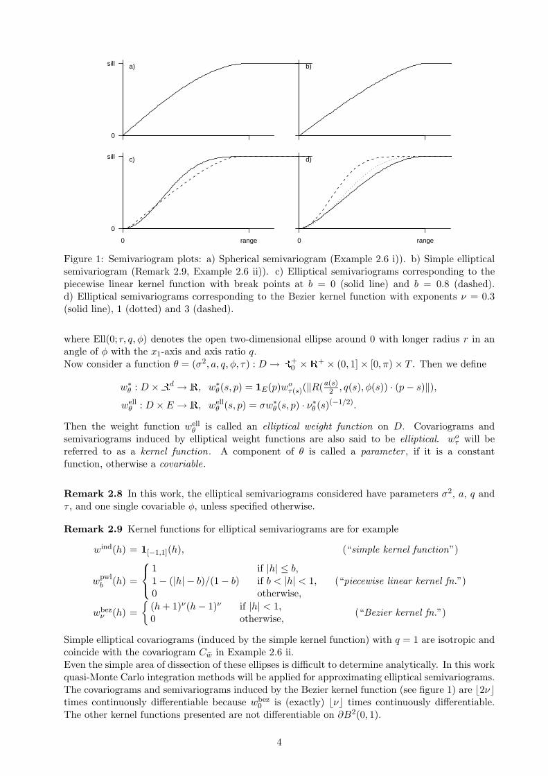
Figure 1: Semivariogram plots: a) Spherical semivariogram (Example 2.6 i)). b) Simple ellipticalsemivariogram (Remark 2.9, Example 2.6 ii)). c) Elliptical semivariograms corresponding to thepiecewise linear kernel function with break points at b = 0 (solid line) and b = 0.8 (dashed).d) Elliptical semivariograms corresponding to the Bezier kernel function with exponents ν = 0.3(solid line), 1 (dotted) and 3 (dashed).

where Ell(0; r, q, φ) denotes the open two-dimensional ellipse around 0 with longer radius r in anangle of φ with the x1-axis and axis ratio q.Now consider a function θ = (σ2, a, q, φ, τ) : D → R

+0 ×R+ × (0, 1]× [0, π)× T . Then we define

w∗θ : D ×Rd → R, w∗θ(s, p) = 1E(p)woτ(s)(‖R(a(s)2 , q(s), φ(s)) · (p− s)‖),

wellθ : D × E → R, well

θ (s, p) = σw∗θ(s, p) · ν∗θ (s)(−1/2).

Then the weight function wellθ is called an elliptical weight function on D. Covariograms and

semivariograms induced by elliptical weight functions are also said to be elliptical. woτ will bereferred to as a kernel function. A component of θ is called a parameter , if it is a constantfunction, otherwise a covariable.

Remark 2.8 In this work, the elliptical semivariograms considered have parameters σ2, a, q andτ , and one single covariable φ, unless specified otherwise.

Remark 2.9 Kernel functions for elliptical semivariograms are for example

wind(h) = 1[−1,1](h), (“simple kernel function”)

wpwlb (h) =

1 if |h| ≤ b,1− (|h| − b)/(1− b) if b < |h| < 1,0 otherwise,

(“piecewise linear kernel fn.”)

wbezν (h) =

(h+ 1)ν(h− 1)ν if |h| < 1,0 otherwise,

(“Bezier kernel fn.”)

Simple elliptical covariograms (induced by the simple kernel function) with q = 1 are isotropic andcoincide with the covariogram Cw in Example 2.6 ii.Even the simple area of dissection of these ellipses is difficult to determine analytically. In this workquasi-Monte Carlo integration methods will be applied for approximating elliptical semivariograms.The covariograms and semivariograms induced by the Bezier kernel function (see figure 1) are b2νctimes continuously differentiable because wbez

0 is (exactly) bνc times continuously differentiable.The other kernel functions presented are not differentiable on ∂B2(0, 1).

4

The following example shows how the class of elliptical semivariograms can be extended, and howparameters and covariables can be chosen in order to represent qualitative knowledge of the geologicprocesses to model.

Example 2.10 (Modeling soil loss by water run-off) Soil erosion by water run-off is a geo-morphological process that basically depends on morphology, vegetation, land use, soil propertiesand precipitation regime. At a small scale, however, the size of the catchment area and the slope’sinclination are the most important factors that influence soil erosion. The soil loss at one pointdepends on the soil loss uphill in the same catchment area, and little correlation with soil loss onthe other side of a ridge or on the opposite side of a valley can be assumed.For a point s ∈ D, let A(s) ⊂ R

2 denote its catchment area. Then a weight function w onD × Rd with suppw(s, ·) = A(s) incorporates our knowledge of the relation between soil erosionand morphology.i) As an example, we define a weight function by (the normalization of)

wθ(s, p) = wellθ (s, p)1A(s)(p), θ = (θ,1A(·)),

where wellθ is an arbitrary elliptical weight function with covariable a : s 7→ 2 supp∈A(s) ‖p− s‖ and

parameters σ2 and τ , the axis ratio q = 1 being constant and hence φ without any effect.The catchment area of a point can be determined by digital terrain modeling, and a large numberof expensive GIS calls to evaluate 1A(s)(p) is necessary to approximate the induced semivariogramby numerical integration.ii) A computationally less demanding method is the following, which approximates wθ quite well insufficiently regular relief. Let R(s) be the shortest distance to the ridge that lies uphill from s, andlet φ(s) ∈ [0, 2π) denote the gradient of topography at s expressed as an angle, and δ(s) ∈ (0, π]an opening angle. Then for an arbitrary elliptical weight function well

θ with q = 1 and covariablesa = 2R and φ, we take (the normalization of)

w′θ(s, p) = well

θ (s, p)1Sec(s;φ(s),δ(s),a(s)/2)(p),

where Sec(s; a(s)/2, φ(s), δ(s)) ⊂ B2(s, a(s)/2) denotes the disc sector with opening angle δ(s) andradius a(s)/2 oriented according to φ(s). The opening angle δ(s) could for example be constant ora function of local curvature at s.

2.3 Modeling Boundaries between Subprocesses

In many geostatistical applications we find the following situation: The parameter set D of theprocess Z of interest decomposes into η disjoint subsets D1, . . . , Dη ⊂ D such that the subprocessesZ1 := Z|D1 , . . . , Zη := Z|Dη have little or no correlation between each other. Instead of studyingeach subprocess separately, one might wish to study the process Z as a whole.Let wo1, . . . , w

oη be weight functions on D×R2. We consider the following situations (i = 1, . . . , η):

“strong boundaries”: w∗i (s, p) := woi (s, p)1Di(s)1Di(p), C∗ =∑

k Cw∗i ,“ordinary boundaries”: wi(s, p) := woi (s, p)1Di(s), C =

∑k Cwk ,

“soft boundaries”: w#(s, p) :=∑

k woi (s, p)1Di(s), C# = Cw# .

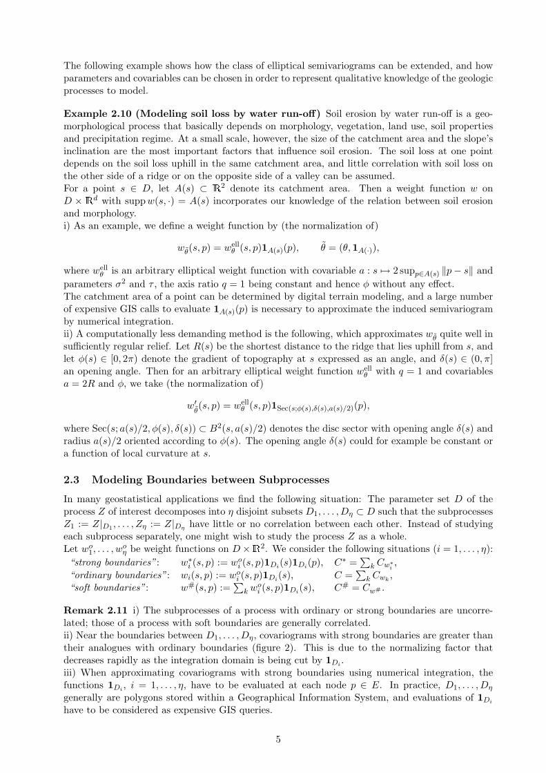
Remark 2.11 i) The subprocesses of a process with ordinary or strong boundaries are uncorre-lated; those of a process with soft boundaries are generally correlated.ii) Near the boundaries between D1, . . . , Dη, covariograms with strong boundaries are greater thantheir analogues with ordinary boundaries (figure 2). This is due to the normalizing factor thatdecreases rapidly as the integration domain is being cut by 1Di .iii) When approximating covariograms with strong boundaries using numerical integration, thefunctions 1Di , i = 1, . . . , η, have to be evaluated at each node p ∈ E. In practice, D1, . . . , Dη

generally are polygons stored within a Geographical Information System, and evaluations of 1Dihave to be considered as expensive GIS queries.

5

0 Di − Dj

0

σ2

Figure 2: Left: Covariograms with ordinary (solid line) and strong boundaries (dashed) near theboundaries. Right: The covariogram from Example 2.12 with soft boundaries.

Example 2.12 (Soft boundaries) Suppose D1 ∪ D2 = D, D1 ∩ D2 = ∅, and let C denote acovariogram with soft boundaries between D1 and D2 induced by a weight function

wpwl(1,a1,1,0)(s, p)1D1(s) + wpwl

(1,a2,1,0)(s, p)1D2(s)

(cf. Definition 2.7, Remark 2.9), where a1 < a2 are different range parameters. This may producea covariogram as shown in figure 2. It will generally not be desirable to introduce a positivecorrelation C(s, t) for s ∈ A1 and ‖t− s‖ > a1, as seen in the figure.

Remark 2.13 (Smooth transitions) The problem encountered in Example 2.12 with soft bound-aries may be avoided by allowing the weight function’s parameter θ ∈ Θ to vary smoothly in space,i. e. modeling it as a covariable.

2.4 Generic Stationarity: towards Stationarizing Instationarity

By construction the (generally non-geometrical) anisotropy of elliptical covariograms can be con-sidered as rather regular because it is determined by the direction φ(s), s ∈ D, of local anisotropy,which is assumed to be known. Therefore we want to introduce a concept that is more generalthan that of stationarity and includes the elliptical case and other situations with “understandable”instationarities.

Remark 2.14 In a more general setting than in the preceding example, we consider processesthat are embedded within a geological environment. The covariogram of such a process should bea function of local geology, we write

C(s, t) = Cg(s, t; g(·)).

We wish to model the function Cg that maps local geology to the proces’ covariogram. Theresulting covariogram is no longer stationary, but depends on local geology. However, some degreeof stationarity remains, since the physical laws reflected in a model for Cg are the same at anyplace. In particular, we assume that we would get the same covariogram in another place, if wehad the same geology there:

C(s+ h, t+ h) = Cg(s, t; Φ(·+ h)).

Example 2.15 Let Z be a process on D = R2 with elliptical covariogram C with parameter θ ∈ Θand direction of local anisotropy φ : R2 → [0, π). Then for all s, t, h ∈ R2 with φ(s) = φ(s+h) andφ(t) = φ(t+ h) it holds

C(s, t) = C(s+ h, t+ h). (3)

That is, it holds “something like” a stationarity property conditional on the direction of localanisotropy φ.

6

However, there will probably exist points s+h′, t+h′ ∈ R2 with φ(s) 6= φ(s+h′) or φ(t) 6= φ(t+h′). Ifwe go beyond the covariogram itself and study the way how its generation depends on the covariableφ, we will find out that for all s, t ∈ R2, we have

∀h ∈ R2 : C(s+ h, t+ h) = Cg(s, t;φ(·+ h)), (4)

where the function Cg : R2 ×R2 × φ(·+ h′) : h′ ∈ R2 → R, is defined by

Cg(s, t;φ(·+ h)) =σ2

ν

∫R2

woθ(‖R(φ(s+ h); θ)(p− s)‖)woθ(‖R(φ(t+ h); θ)(p− t)‖dp (5)

with an appropriate normalizer ν. Thus, C(s+h, t+h) only depends on s, t and the moved geologyrepresented by φ(·+ h).The last two equations suggest that “if we had φ(s) = φ(s+h′) and φ(t) = φ(t+h′), then we wouldget C(s, t) = C(s+ h′, t+ h′)” —a hypothetic version of (3), based on our belief in the validity ofthe law expressed in (4) and (5).The following definition reflects this concept in a precise way.

Definition 2.16 (Generic stationarity) Consider a process Z on D = Rd with covariogram C,semivariogram γ and mean m, and let g : Rd → T be a mapping onto an arbitrary set T . Then wedefine:

i) The process Z is strongly generically stationary with respect to g, if there exists a functionPg such that

∀B ∀h ∈ Rd : P (Z·+h ∈ B) = Pg(B, g(·+ h)).

Or, more precisely,

∀B ∈ A ∀h ∈ Rd : P (Bh) = Pg(B; g(·+ h))

where Bh = ω ∈ Ω : ∃ ω ∈ B : Z·(ω) = Z·+h(ω), (Ω,A, P ∈ P) is a statistical model andPg a mapping g : Rd → T → P.

ii) Γ ∈ C, γ is generically stationary with respect to g, if there exists a function Γg such that

∀ s, t, h ∈ Rd : Γ(s+ h, t+ h) = Γg(s, t; g(·+ h)).

iii) If there exists a function mg such that

∀ s, h ∈ Rd : m(s+ h) = mg(s, g(·+ h)),

then m is generically stationary with respect to g, and Z is first-order generically stationarywith respect to g.

iv) Z is (second-order or weakly) generically stationary, if m and C are, and the process isintrinsically generically stationary, if m and γ are generically stationary.

Pg, Γg and mg are called influence laws of generic stationarity, and g an influence function.

Remark 2.17 Generic stationarity says that the distribution laws of Zs and Zt, s, t ∈ D, are orbecome the same, if local geology around s and t are the same or are “forced” to be the same.That is, generic stationarity assumes that there is something like a law of nature that determinesthe distribution of a random variable given the local geology g. Depending on how we choosethe function g, generic stationarity becomes a triviality or an instrument that describes how adistribution law is determined by the environment.

7

Example 2.18 i) Elliptical semivariograms are stationary with respect to their covariables.ii) If Z is a process with a deterministic trend, Zs = Ys + βTf(s) for all s ∈ D, where (Ys)s∈D is azero-mean stationary process, then Z is generically stationary with respect to g = βTf .

Remark 2.19 Consider a generically stationary process Z with influence function g. g can taketwo “extreme” cases: i) g is constant. Then Z is stationary in the usual sense. ii) g is bijective.Then there is no condition on the distribution of Z. One could say that a constant influencefunction gives no information on local geology, while a bijection contains complete knowledge oflocal geology and hence explains arbitrary spatial variation of the process’ distribution. Betweenthese two extremes, there is a broad variety of meaningful influence laws (see the examples above).

3 Geostatistics and GIS

Our goal is to implement instationary geostatistical methods fully within a general-purpose dataanalysis environment, and to provide direct access to this functionality from an exemplarily chosenGIS. The applicability of the geostatistical routines will however not be restricted to a specific GISsoftware.For the implementation of geostatistical methods, the data analysis language and environment Rwas chosen. R offers a simple and effective programming language that includes conditionals, loopsand user defined functions, and there exists a kind of object-oriented design. A great variety ofstatistical models and methods is also available, among them linear models, clustering and time-series analysis.The R environment is open source. Open-source software is not only cheaper than commercialalternatives; the main advantage of using it is related to the efficiency of problem-solving anddebugging within a community of users. Furthermore, full access to source code makes it possibleto find out details of the implementation that are not documented in the manuals (Bivand 1999).R differs very little from the language S and its derivative S-PLUS.As GIS platform, the commercial software ArcView 3.1 was chosen, because of its wide use in thepublic and private sector. However, a relatively small amount of code has to be generated in orderto create an interface for a different GIS environment.In total, about 100 KB of R code, 30 KB of C code and 30 KB of AVENUE source code wereproduced. The code was developed for R 1.2.2, Microsoft Visual C++ 5.0 and ArcView 3.1 andused within a Microsoft Windows 2000 5.0 / NT 4.0 client–server environment on Pentium II familyprocessors at Freiberg University.Source code and further documentation can be obtained from the authors.

3.1 Approximating Semivariograms with Quasi-Monte Carlo Integration

When we fit a semivariogram model or do kriging, a great number of semivariogram evaluationsis needed, which are generally computed by approximating the integral in (1), if a model of theelliptical class is used. Quasi-Monte Carlo techniques possess good asymptotic properties and areoften preferred to numerical methods, especially in higher-dimensional integration. For details ofquasi-Monte Carlo methods, we refer to Niederreiter (1992), Evans and Swartz (2000) and Presset al. (1992).Consider a covariogram C induced by a weight function w with bounded support. We want to ap-proximate (non-zero values of) C(s, t), s, t ∈ D, E = Rd, i. e. the integral of fs,t(p) = w(s, p)w(t, p)over a suitable interval A ⊃ supp fs,t = suppw(s, ·) ∩ suppw(t, ·). We use the quasi-Monte Carloapproximation

CK(s, t) :=λd(A)K

K∑i=1

fs,t(pi) ≈ C(s, t)

with p1, . . . , pK ∈ A. Using low-discrepancy sequences of nodes, the error of the quasi-Monte Carloapproximation is of the order of (logK)d/K. Such a sequence is the Sobol sequence, which is used

8

in this work in a modified version proposed by Antonov and Saleev. The implementation of thegenerator is taken from Press et al. (1992).We use an algorithm that computes the quasi-Monte Carlo approximation of covariograms inducedby elliptical weight functions. Both algorithms support ordinary and strong boundaries. Thealgorithm uses nodes that are created a priori and recycled in every evaluation of C(si, sj). Thus,the number of oracle calls 1Di(p) can be reduced significantly. Furthermore, all K oracle calls canbe performed at once, e. g. by just one call to a GIS.

3.2 Minimizing the Mean Squared Error

Remark 3.1 (Minimization in R) In R, non-linear minimization can be carried out using aNewton-type algorithm available through the function nlm. In this work, nlm is used for minimiz-ing mean squared error functions. It computes numerical derivatives of the target function andconsequently needs a high number of (expensive) function evaluations. Derivative-free techniquesmay therefore be more efficient.

Observation 3.2 The mean squared error function corresponding to the simple elliptical semi-variogram (Example 2.6, Remark 2.9) usually possesses local minima. This is related to the corre-sponding semivariogram approximation being discontinuous with respect to the range parameter.In contrast, the piecewise linear elliptical kernel function (Remark 2.9) with breaking point pa-rameter b close to 1 is almost identical to the simple one, but it is continuous in its argumentsand hence the corresponding semivariogram approximation is continuous with respect to its rangeparameter. The minimization of mean squared error performed quite well with this semivariogramapproximation using b = 0.95, for example, since small local minima are smoothed out now.

3.3 Implementation of Geostatistical Methods

Because of our emphasis on generically stationary processes, the generated R and C code will becalled MoGeS, which stands for “Modeling Generic Stationarity”.The current implementation deals with the following geostatistical tasks1:Semivariogram modeling: Select from a variety of stationary and instationary models, determinecovariables, assign fixed values to parameters, and add semivariograms. Furthermore, visualizeanisotropic semivariograms along a given path.Semivariogram fitting: Estimate semivariogram parameters by minimizing the mean squarederror function.Kriging: Perform universal and ordinary kriging.Interaction with a GIS: Read and write geostatistical datasets in an interchangeable file format.Simulation of datasets: Create random data to a given semivariogram.

The specific tasks result in a series of routines, most of them being represented as methods of objectclasses.Semivariogram (and covariogram) models are represented as objects of class sv, which is anabstract parent of svfn, svc and csv representing different levels of specification and aggregation.Semivariogram models “know” which parameters they need, if they are stationary etc.Parameters are modeled as an independent object class param in order to allow meta-data suchas semantics or the range of valid parameter values to be handled consistently together with theparameter vector itself.Geostatistical data consists of locations, measurements and covariables stored in a svm.dataobject.

1Furthermore, fitting of semivariograms in the presence of trend was implemented, which is discussed in thepresentation by K. G. van den Boogaart and A. Brenning: Why is Universal Kriging Better than IRFk-Kriging:Estimation of Variograms in the Presence of Trend.

9

Figure 3: Semivariogram fitting within ArcView using the ArcView/MoGeS interface.

Figure 4: R code produced by the ArcView/MoGeS interface in an example situation.

[...] # initialization

###### read geostatistical data

d <- read.svm.data( file="z:/scripts/humid.csv",

xnames="x", ynames="y", znames="Humo", gnames=c("orientation") )

n <- nrow(d$xy)

###### specify a semivariogram model

fpa <- param( c(0.9), # we have one fixed parameter

nm = c("break.elliptical.pwlinear.global"), sem = c("break") )

pa.al <- setnames( c("sill.elliptical.pwlinear.global", # parameter aliases

"range.elliptical.pwlinear.global","q.elliptical.pwlinear.global",

"break.elliptical.pwlinear.global"),

c("sill","range","q","break") )

g.al <- setnames( c("orientation.elliptical.pwlinear.global"), # covariable aliases

c("orientation") )

svc1 <- svc( svfn.elliptical.pwlinear.global, # a ‘svc’ semivariogram object

fix.param=fpa, param.alias=pa.al, g.alias=g.al )

sv <- csv( list( svc1 = svc1 ) ) # this is our composed ‘csv’ semivariogram object

###### fit the semivariogram model:

start <- param( c(5,10000,0.7), # starting ‘param’eter object

nm = c("sill.elliptical.pwlinear.global","range.elliptical.pwlinear.global",

"q.elliptical.pwlinear.global"),

sem = c("sill","range","q") ) # parameter semantics

smp <- NULL

if (needs.smp.data(sv)) # generate a priori nodes for quasi-monte carlo integration

# the ‘Rmax’ argument must be sufficiently large!

smp <- smp.data(d, Rmax=1.7*max(getrange(sv,start))/2, N=5000)

svmfit <- svm(sv,d=d,param=start,smp=smp,trend=FALSE) # fit the model

print(summary(svmfit))

10

a)

c)

b)

A1 A1

A2

Figure 5: The situation of the simulated dataset with local anisotropy: Two independent subpro-cesses on A1 and A2 are considered (left). The curves represent the paths for which semivariogramsare shown in figure 6. The sketch at the right visualizes the directions of local anisotropy.

Nodes are generated a priori for quasi-Monte Carlo integration and stored in a smp.data object.Fitted semivariogram models are represented by a svm object, which contains information onparameter estimates and other results of mean squared error minimization trials. (They are handledin a similar way as fitted linear models in R.)

3.4 Implementation of a GIS Interface

The ArcView/MoGeS interface performs geostatistical modeling in four steps:Export data: Select a set of points and corresponding data from a point theme and its databaseor table (in ArcView terminology) and convert it to a text file format that can be read by MoGeS.Specify a semivariogram model: Select semivariogram models, and link covariables with fieldsin the theme’s database. If desired, assign fixed values to parameters or identify parameters.Fit the semivariogram model: Choose starting parameter values, and perform the fittingthrough a call to the R environment. See figure 3 for a screen shot and figure 4 for an exam-ple of R code generated by the ArcView/MoGeS interface.Perform kriging: Select measurement and prediction locations, export the corresponding dataand perform kriging by calling the R environment.The ArcView/MoGeS interface is a collection of AVENUE scripts that perform these tasks. Itis accessible through commands added to the Theme menu (see figure 3). The scripts of coursedo not cover the complete MoGeS functionality available within R. Nevertheless, the problemsmentioned above can be solved more easily than by hand, since R code is generated and executedautomatically, and a user who is familiar with R will be able to add flexibility by modifying thiscode or doing additional analyses using the whole spectrum of R and MoGeS functions.The AVENUE scripts model parameter vectors, names, aliases and semantics just as MoGeS does,however as seperated lists rather than object classes or names vectors.In its current implementation, the ArcView/MoGeS interface strongly depends on the MoGeSimplementation (i. e. its function identifiers, argument names etc.), which makes it very sensibleto small changes in MoGeS. This could be overcome by using a meta-language for geostatisticalmodeling that makes for example model specifications independent of the actual implementationthat executes it.

4 Application: A Simulated Dataset in Complex Geology

We consider a Gaussian process Z on D = [0, 1]2 made up of two independent subprocesses Z1 on A1

and Z2 on A2 with location-dependent directions of anisotropy φ(s) (see figure 5 for illustration).

11

+

++

+

+++

+

+

+

+

+

++

++++

+

+

+

+

++++

++++++

++

+

+++

+

+

+

+

+++

+++

+++

+

++

+

+

++

+

+

++

++++++++

++

+

+

+

0.00 0.04

0.0

1.9

0.00 0.13

0.0

1.7

a)b)

c)

Figure 6: Left: Empirical semivariogram and the fitted spherical semivariogram with sill 1.90 andrange 0.04.Right: The fitted “true” semivariogram model, evaluated along the three paths shown in Figure 5:a) following the local direction of anisotropy in A1; b) orthogonal to anisotropy in A1; c) followinganisotropy in A2.

We select a constant mean m = 5 and elliptical semivariograms with a piecewise linear kernelfunction and parameters θT1 = (σ2

1, a1, q1, b) = (1, 0.2, 0.6, 0.6) on A1 and θT2 = (0.8, 0.1, 0.4, 0.95)on A2, and on A2, we also add a nugget effect with parameter σ2

nug(2) = 0.4. The directions ofanisotropy on A1 and A2 are defined by polynomials and visualized in figure 5.A geologic setting that hosts such a process could for example be the following: Suppose that Zrepresents some (lithogenic) soil property. On A2, geologically young river sediments with strongfabric orientation down-stream and high local irregularity host the subprocess Z2 with analogousproperties (anisotropy with q2 = 0.4, small range, nugget effect). On A1, things are smoother(a1 = 2a2, no nugget effect), but oblique sediment layers with folding structures originate ananisotropy (q1 = 0.6).A total of n = 259 locations was generated, 170 of which are uniformly distributed over A1, andthe remaining 89 are uniformly distributed over A2. Then realizations of Z at these points weresimulated using a Cholesky decomposition of the covariance matrix.Kriging was performed on a 60 × 60 grid using 10 000 a priori nodes. The computation of all thekriging predictions presented below took about a quarter of an hour in total, and each fitting triala few minutes, depending on the number of iterations needed.For comparison with more sophisticated models, we fitted stationary models with and withoutanisotropy, first of all the spherical semivariogram model using four different starting values. Alltrials succeeded and yielded practically the same estimates, namely a sill of 1.90 and a range of0.039 (mse: 32.08). (See figure 6 for a comparison with the empirical semivariogram.) However,fitting an elliptical semivariogram with a piecewise linear kernel function (with b = 0.7) and fixeddirection of (geometrical) anisotropy did not yield consistent results for various choices of startingvalues and (fixed) orientation parameters.Finally we fitted the “true” semivariogram model. Due to the high number of parameters, fittingtook several steps, fixing some parameters at each step.Comparing fitted and true parameters,

σ21 a1 q1 b1 σ2

2 a2 q2 b2 σ2nug(2)

fitted 1.70 0.13 0.55 (0.70) 2.27 0.12 0.34 (0.70) 0.06true 1.00 0.20 0.60 0.95 0.8 0.10 0.40 0.95 0.40

we observe that the fitted nugget effect almost vanishes, the sill parameters were overestimated,axis ratios were estimated quite well, and the range in the smoother area A1 was underestimated.Overestimation of the sill may be caused by an additional randomness due to integration errorsduring simulation.See figure 6 for some sample plots of the fitted semivariogram along the paths shown in figure 5.

12

x x

x x

Figure 7: Kriging surfaces using the true semivariogram (top left), using the fitted genericallystationary model (top right), using a fitted spherical semivariogram (sill 1.90, range 0.039; bottomright), and using a spherical semivariogram with sill 1.90 and range 0.13 (bottom left).

Note that these plots are representative in the sense that any semivariogram evaluation alonganisotropy direction within A1 will look like graph a), etc. This is due to the generic stationarityproperty of elliptical semivariograms.Our next aim is to compare kriging predictions obtained with different fitted models. We use thefollowing semivariograms:

• the true semivariogram,

• the fitted semivariogram consisting of piecewise linear elliptical semivariograms on A1 andA2 plus a nugget effect on A2,

• the fitted spherical semivariogram with sill 1.90 and range 0.39, and

• a spherical semivariogram with sill 1.90 and the (more reasonable) range 0.13 taken from thefitted semivariogram with local anisotropy.

Kriging results are shown in Figure 7. It can clearly be seen that both predictions based onspherical semivariograms do not reflect the strong anisotropies present in our dataset, whereas thefitted generically stationary model with anisotropies leads to predictions that are very close to thoseobtained with the true semivariogram.

5 Conclusions

The construction method presented in this work has shown to be a useful instrument for incorpo-rating knowledge of local geology as stored in a GIS into semivariogram models. Many situationsof local anisotropy can be modeled using the class of elliptical semivariograms, which was studiedin detail. Using the code developed for the present work, such models were successfully fitted, and

13

in an example situation it could be seen that the corresponding kriging results are also consistentwith our knowledge of local anisotropy of the process, in contrast to isotropic or geometricallyanisotropic semivariograms.The study of the class of elliptical covariogram models motivated the introduction of the concept ofgeneric stationarity. This concept reflects our belief in the existence of natural laws that determinea process’ distribution law depending on local geology. The less knowledge of local geology isnecessary to determine the distribution law, “the more stationary” is the process. Thus, genericstationarity becomes a means for stationarizing instationarity conditional on local geology.First practical results were obtained by modeling the influence of local geology by means of generi-cally stationary semivariograms in some cases of particular interest. However, it remains for futurework to investigate and apply other generically stationary models to geological problems involvingdata from GIS.

References

Bivand, R. S. (1999): Integrating GRASS 5.0 and R: GIS and modern statistics for data analysis. In:Proc. 7th Scandinavian Research Conf. on Geogr. Information Science, pp. 111-127. Aalborg,Denmark.

Cressie, N. A. C. (1993): Statistics for spatial data. Wiley, New York.

Evans, M., and T. Swartz (2000): Approximating integrals via Monte Carlo and deterministicmethods. Oxford Univ. Press, Oxford et al.

Goovaerts, P. (1997): Geostatistics for natural resources evaluation. Oxford University Press, NewYork et al.

Niederreiter, H. (1992): Random number generation and quasi-Monte Carlo methods. CBMS–NSFregional conference series in applied mathematics. SIAM, Philadelphia.

Press, W. H., S. A. Teukolsky, W. T. Vetterling and B. P. Flannery (1992): Numerical recipes inC. 2nd ed., Cambridge Univ. Press, Cambridge et al.

Stein, M. L. (1999): Interpolation of spatial data: some theory for kriging. Springer, New York.

van den Boogaart, K. G. (1999): A new possibility for modelling variograms in complex geology.Proc. of StatGIS Klagenfurt 1999, to appear.

Wackernagel, H. (1998): Multivariate geostatistics: an introduction with applications. Springer,Berlin et al.

14