1

George Mason University Department of Civil, Environmental and Infrastructure Engineering

Dr. Celso Ferreira

Prepared by Lora Baumgartner

Exercise Topic: Getting started with HEC –RAS ____________________________________________________________________________________________________________

Objective: Create a HEC-RAS model of the George Mason University watershed using HEC-RAS.

**Refer to the HEC-RAS User Manual for definitions and context of the steps and tools in this tutorial, found in the Help Menu of the RAS toolbar.*

Tutorial Cross Section Data provided in .TXT appendix.

Versions used for this tutorial: HEC-RAS 4.1.0

2

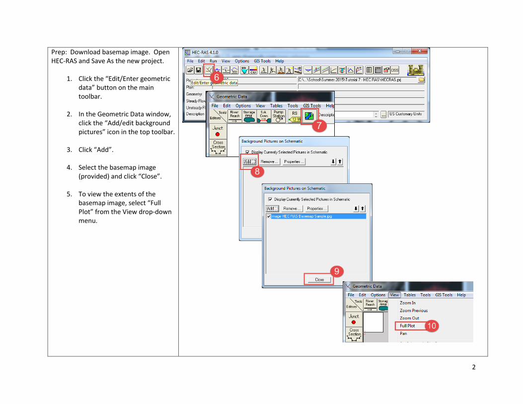
Prep: Download basemap image. Open HEC-RAS and Save As the new project.

1. Click the “Edit/Enter geometric data” button on the main toolbar.

2. In the Geometric Data window, click the “Add/edit background pictures” icon in the top toolbar.

3. Click “Add”.

4. Select the basemap image (provided) and click “Close”.

5. To view the extents of the basemap image, select “Full Plot” from the View drop-down menu.

3

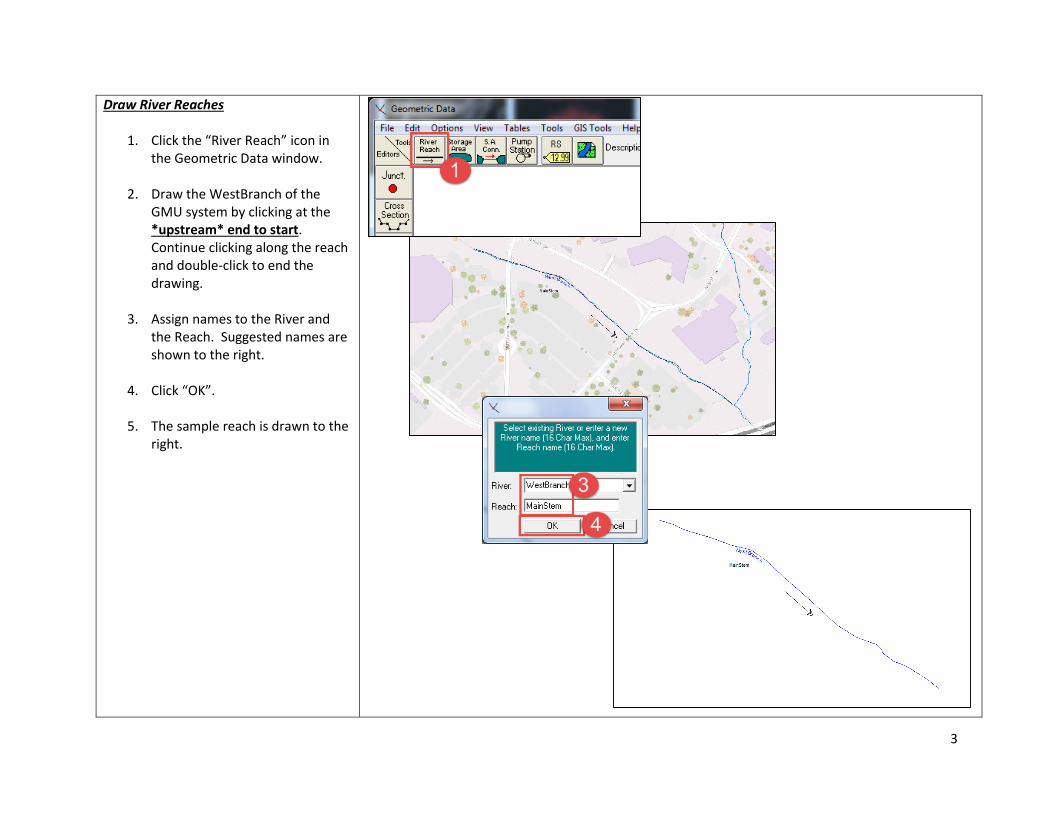
Draw River Reaches

1. Click the “River Reach” icon in the Geometric Data window.

2. Draw the WestBranch of the GMU system by clicking at the *upstream* end to start. Continue clicking along the reach and double-click to end the drawing.

3. Assign names to the River and the Reach. Suggested names are shown to the right.

4. Click “OK”.

5. The sample reach is drawn to the right.

4

6. Repeat the reach drawing for the

EastBranch of the GMU system. *Doubleclick to end the EastBranch on top of the end of the WestBranch.

7. Click “OK”.

8. A junction between the West and

East branches will be automatically created. Name the junction.

9. Click “OK”.

5

Build Cross Sections

1. Click the “Cross Section” icon in the left toolbar.

2. Select the Outlet reach from the River drop-down menu.

3. Select “Add a new Cross Section” from the Options drop-down menu.

*Cross Sections must be drawn from downstream to upstream.

4. Assign the station number as the

name. Start with the downstream cross section of the Outlet.

5. Click “OK”. Save Geometry data (this is separate from saving project at beginning of exercise).

6

6. Note that the river station of the cross section has been assigned.

7. Enter the Cross Section Coordinates. The Station indicates the x-coordinate of a point within the geometry of the cross section. The Elevation to the right of the Station indicates the corresponding y-coordinate.

8. Enter the Manning’s “n” values for the cross section components. Manning’s “n” values are indicated for the left bank, centerline, and right bank of the stream.

9. Enter the bank stations. Bank stations indicate intersection of bank lines with cross section geometry line.

10. Enter the downstream reach lengths. Lengths to next downstream feature. Differing values indicate that the cross section is offset (the stream makes a bend).

7

11. When all information has been

entered in the Cross Section Data fields, click “Apply Data” in the same window. The cross section geometry, based on the Station and Elevation coordinates provided, is drawn.

8

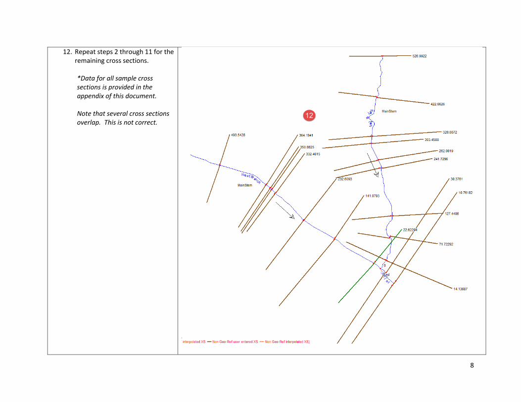
12. Repeat steps 2 through 11 for the remaining cross sections. *Data for all sample cross sections is provided in the appendix of this document.

Note that several cross sections overlap. This is not correct.

9

“Dog-leg” the Intersecting Cross Sections

1. Select “Move Object” from the Edit menu in the Geometric Data window.

2. Drag the overlapping ends of each cross section Choose locations that eliminate overlap while minimizing bend.

10

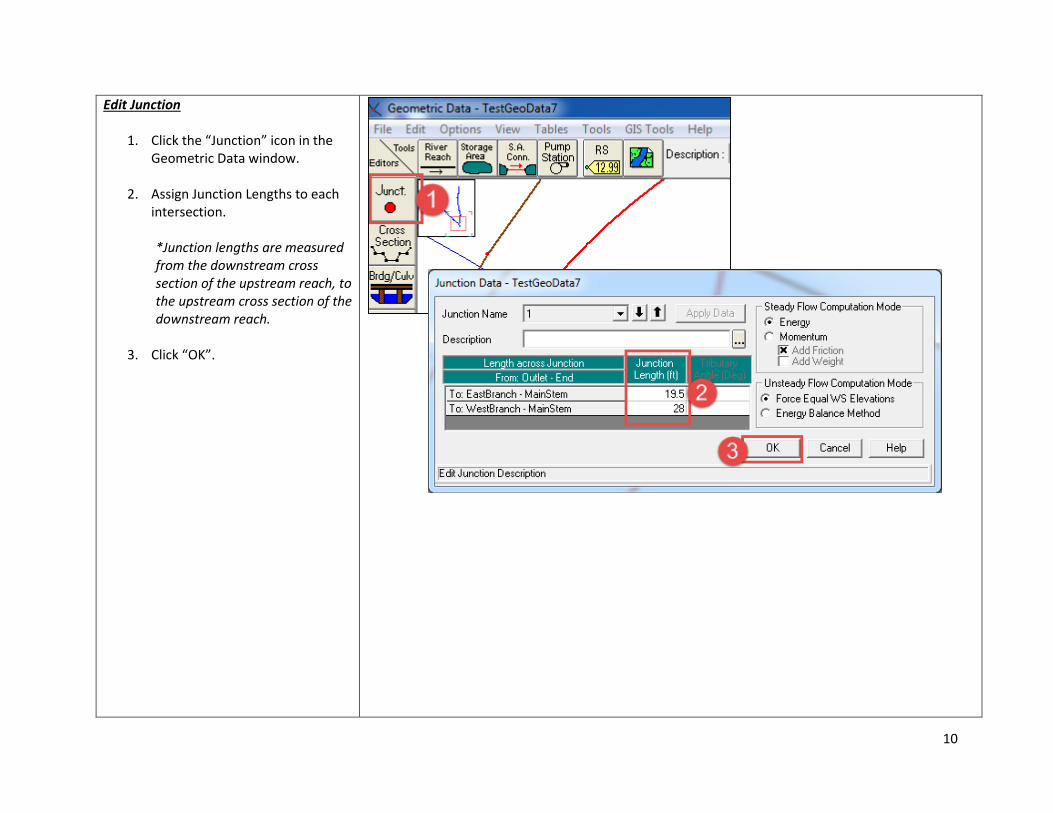
Edit Junction

1. Click the “Junction” icon in the Geometric Data window.

2. Assign Junction Lengths to each intersection.

*Junction lengths are measured from the downstream cross section of the upstream reach, to the upstream cross section of the downstream reach.

3. Click “OK”.

11

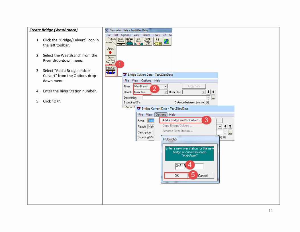
Create Bridge (WestBranch)

1. Click the “Bridge/Culvert” icon in the left toolbar.

2. Select the WestBranch from the River drop-down menu.

3. Select “Add a Bridge and/or Culvert” from the Options drop-down menu.

4. Enter the River Station number.

5. Click “OK”.

12

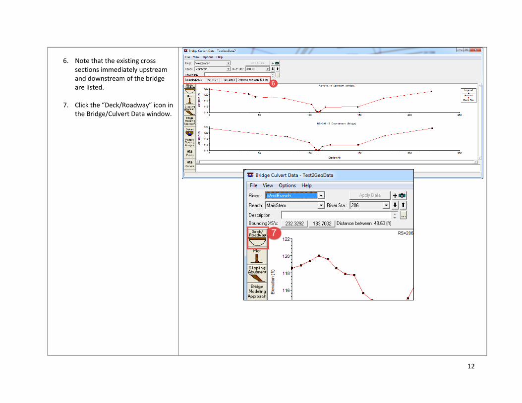
6. Note that the existing cross

sections immediately upstream and downstream of the bridge are listed.

7. Click the “Deck/Roadway” icon in the Bridge/Culvert Data window.

13

8. Enter the distance from the

upstream face of the bridge to the closest upstream cross section.

9. Enter the width of the bridge.

10. Enter the upstream side and downstream side coordinates. “High chord” indicates the y-coordinate of the top of the bridge for the given station. “Low chord” indicates the y-coordinate of the bottom of the bridge for the given coordinate. If value is 0, bridge will be filled in to the ground level.

11. Click “OK”. *The bridge geometry, based on the Station and chord coordinates provided, is drawn.

14

Create Culvert (EastBranch)

1. Still in the Bridge Culvert Data window, select the EastBranch.

2. Select “Add a Bridge and/or Culvert” from the Options drop-down menu.

3. Assign the River Station value and click “OK”.

4. Click on the Culvert icon on the left toolbar.

15

16

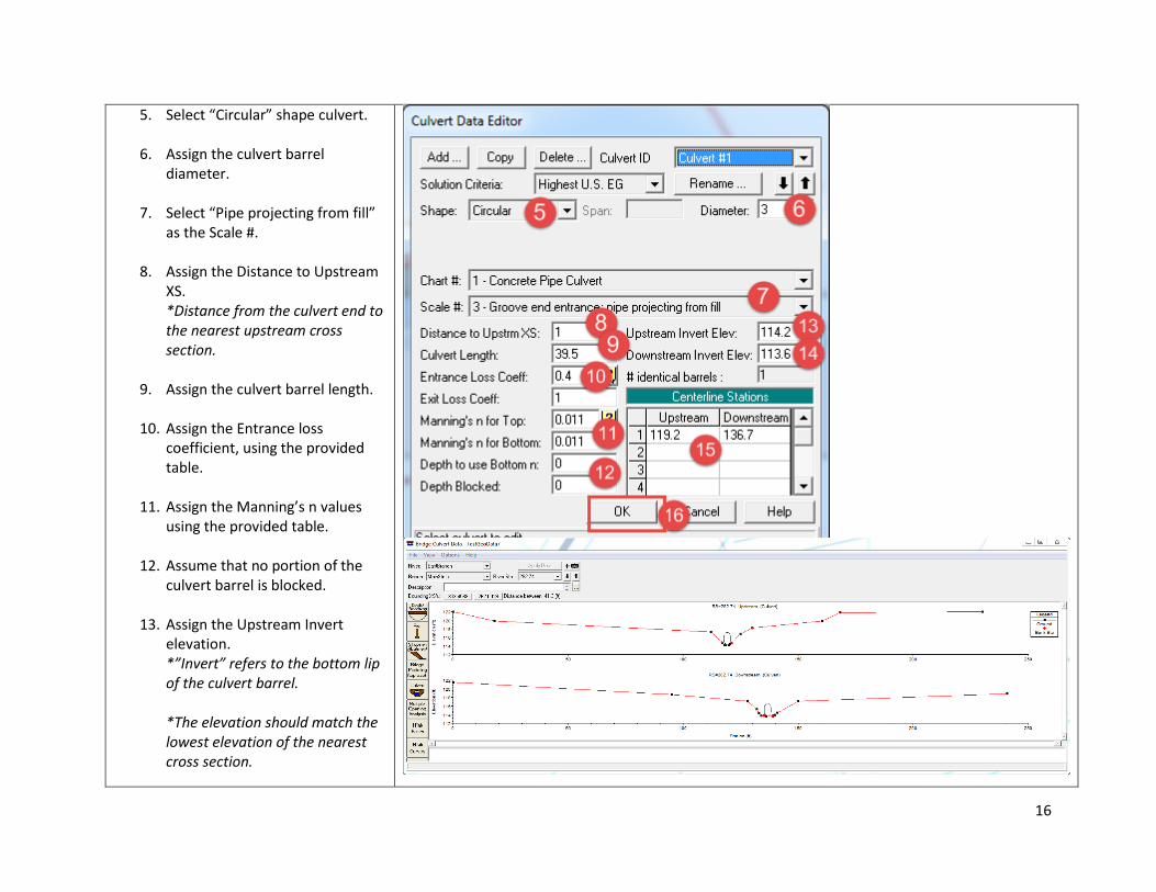
5. Select “Circular” shape culvert.

6. Assign the culvert barrel diameter.

7. Select “Pipe projecting from fill” as the Scale #.

8. Assign the Distance to Upstream XS. *Distance from the culvert end to the nearest upstream cross section.

9. Assign the culvert barrel length.

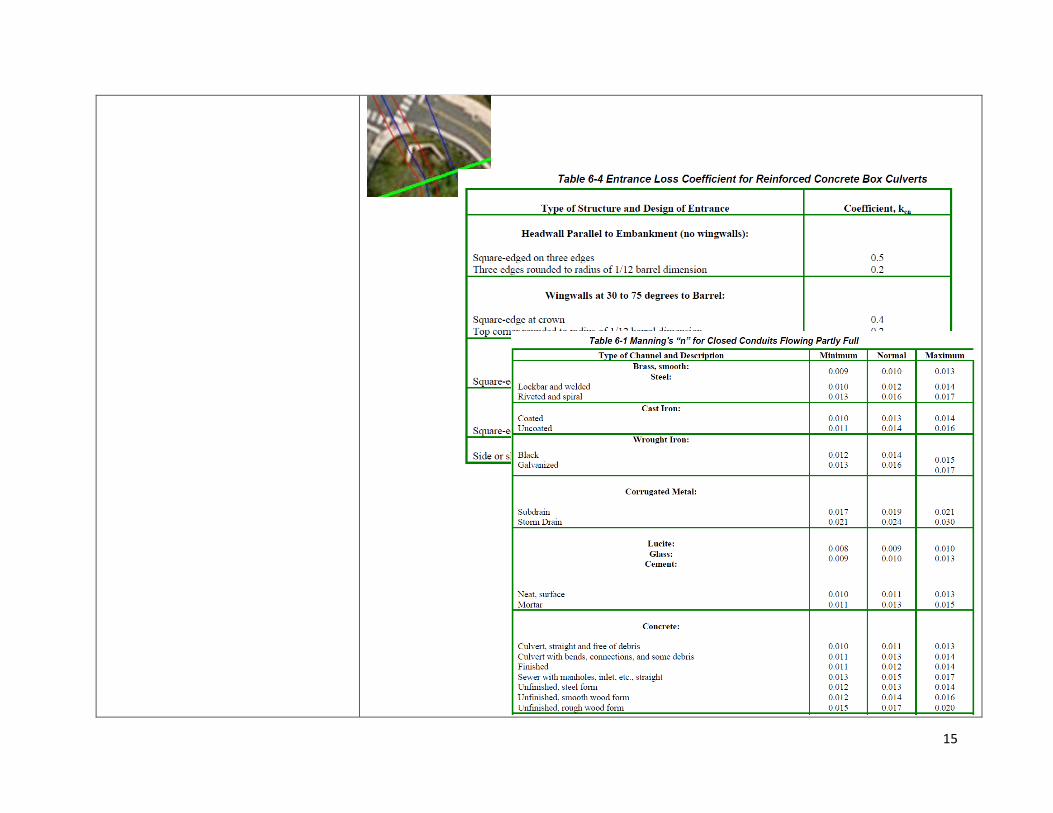
10. Assign the Entrance loss coefficient, using the provided table.

11. Assign the Manning’s n values using the provided table.

12. Assume that no portion of the culvert barrel is blocked.

13. Assign the Upstream Invert elevation. *”Invert” refers to the bottom lip of the culvert barrel. *The elevation should match the lowest elevation of the nearest cross section.

17

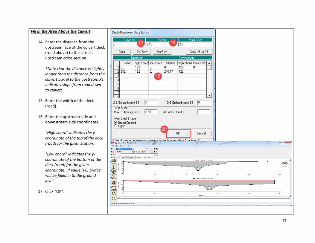
Fill in the Area Above the Culvert

14. Enter the distance from the upstream face of the culvert deck (road above) to the closest upstream cross section. *Note that the distance is slightly longer than the distance from the culvert barrel to the upstream XS. Indicates slope from road down to culvert.

15. Enter the width of the deck (road).

16. Enter the upstream side and downstream side coordinates. “High chord” indicates the y-coordinate of the top of the deck (road) for the given station. “Low chord” indicates the y-coordinate of the bottom of the deck (road) for the given coordinate. If value is 0, bridge will be filled in to the ground level.

17. Click “OK”.

18

*Geometry should look similar to diagram at right at this point.

19

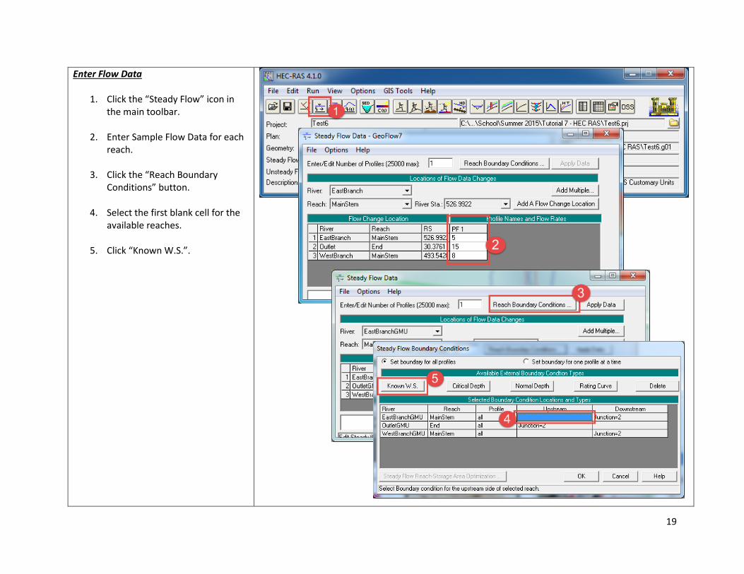
Enter Flow Data

1. Click the “Steady Flow” icon in the main toolbar.

2. Enter Sample Flow Data for each reach.

3. Click the “Reach Boundary Conditions” button.

4. Select the first blank cell for the available reaches.

5. Click “Known W.S.”.

20

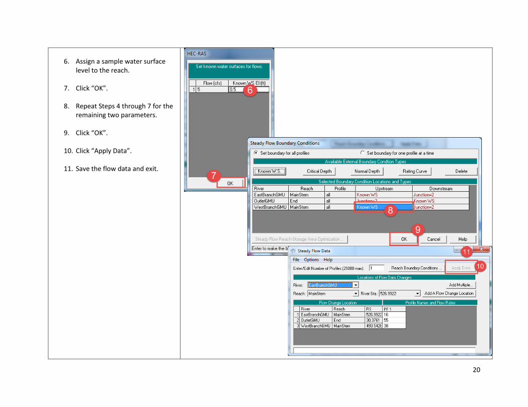
6. Assign a sample water surface

level to the reach.

7. Click “OK”.

8. Repeat Steps 4 through 7 for the remaining two parameters.

9. Click “OK”.

10. Click “Apply Data”.

11. Save the flow data and exit.

21

Simulation Run

1. Click the “Steady Flow Simulation” icon in the main toolbar.

2. Confirm that Subcritical Flow is selected.

3. Click “Compute” to run the simulation.

4. Address any errors; if none, click “Close”.

22

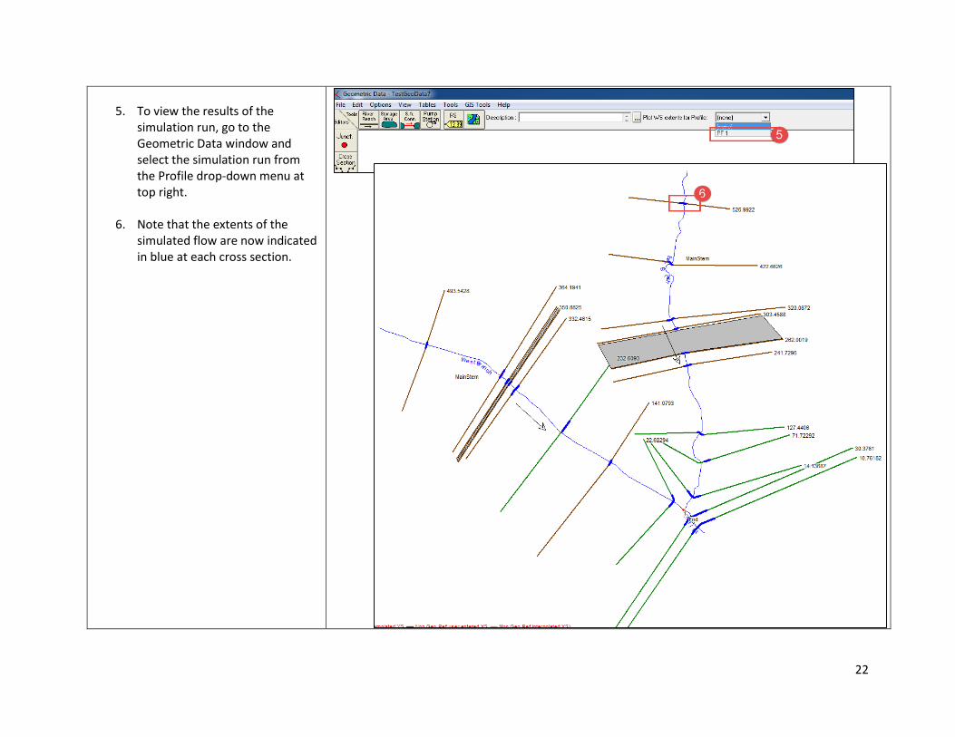
5. To view the results of the

simulation run, go to the Geometric Data window and select the simulation run from the Profile drop-down menu at top right.

6. Note that the extents of the simulated flow are now indicated in blue at each cross section.