geophysical monitoring of leachate recirculation · pdf fileresistivity tomography, ......

GEOPHYSICAL MONITORING OF LEACHATE

RECIRCULATION AT ORCHARD HILLS LANDFILL

PI: Krishna R. Reddy; Co-PIs: Solenne Grellier, Philip Carpenter & Jean Bogner

Final Project Report Submitted To:

Environmental Research and Education Foundation (EREF) Alexandria, VA

Submitted By:

University of Illinois at Chicago Department of Civil and Materials Engineering

2095 Engineering Research Facility 842 West Taylor Street, Chicago, Illinois 60607

May 2009

ii

ACKNOWLEDGEMENTS

This project is a collaborative project between the University of Illinois at Chicago (UIC), Chicago, Illinois; Centre de Recherche pour l’Environnement, l’Energie et le Dechet (CREED), Limay, France; Northern Illinois University (NIU), DeKalb, Illinois; Veolia Environmental Services, Inc., Davis Junction, Illinois; and Landfills+, Inc., Wheaton, Illinois. The financial support provided for this project by the Environmental Research and Education Foundation (EREF) is gratefully acknowledged. This project is a part of comprehensive research program supported by the CREED, National Science Foundation (CMMI Grant #0600441), and Veolia Environmental Services, Inc.

Krishna R. Reddy, Ph.D., P.E.

Principal Investigator University of Illinois at Chicago

iii

EXECUTIVE SUMMARY The main objective of this study was to investigate geophysical techniques that can be useful to monitor bioreactor landfills. Several non-invasive surface geophysics techniques were tested at Orchard Hills landfill located in Davis Junction, Illinois. These techniques included electrical resistivity tomography, electromagnetic surveys, ground penetrating radar, and well logging. Electrical resistivity depends on water content, thus the measured electrical resistivity tomography (ERT) allows determination of spatial distribution of waste moisture (not just isolated locations as with probes). ERT was performed with a Syscal Pro resistivity-meter during several leachate injection periods. From the testing, we observed the leachate distribution along the leachate recirculation lines was not clearly evident, but the leachate distribution around the recirculation line showed a decrease of resistivity around the line. Even though, more comprehensive monitoring are needed, the results of this study showed that ERT method has a great potential to be used as monitoring tool to optimize the leachate recirculation, leading to the best performance of bioreactor landfills. Electromagnetic surveys were performed to monitor the leachate recirculation. EM31 and EM34, both manufactured by Geonics, Ltd. of Mississauga, Ontario, Canada, were used. Frequency-domain EM conductivity measurements were made along the upstream and alongstream lines, as well as some shorter crosslines. The EM31 allowed faster measurements since both transmitting and receiving loops were mounted on one fiberglass tube, and could be operated by one person (one line is acquired in about 20 min), but the investigation depth was less (between 3 and 6 m, according the coil orientation). The EM34, which consisted of two individual loops that required 2 persons to operate, had an investigation depth of 7.5 to 30 m, depending on the configuration and coil spacing (10 or 20 m respectively). One line was acquired in about 40 min. On the Alongstream Line, the HD showed an increase of conductivity compared to the reference after the first 15 m of the line, most likely reflecting the change in slope of the landfill’s surface. The main changes in conductivity occurred just between the first measurement and the reference, as the variations did not change consequently after the first measurement. The variations observed above LRL29 were in the same range as the dispersion. Thus, considering the shallow investigation depth (2.8 m) and the measurement dispersion, it seems that leachate recirculation cannot be seen with the EM31 in the HD orientation. The Ground-penetrating radar (GPR) provides a picture-like display, consisting of radar waveforms plotted as time vs. position (side-by-side) “traces.” The display looks like a geological cross-section, but important differences exist. Some signals on the sections may arise from above-ground reflections. Other distortions may also occur (e.g. diffractions from point reflectors, ringing from multiple reflections, etc.). For this reason apparent reflections are called “events” on the radar sections. Times on GPR sections are usually specified in nanoseconds (ns) – a nanosecond is 1 x 10-9 s. GPR tests conducted over the leachate recirculation cell at Orchard Hills were designed to: (1) determine the penetration depth of GPR signals in highly conductive waste and cover materials, (2) measure the radar wave velocity, and (3) see if the GPR technique could image subsurface targets, such as a leachate recirculation pipe, trench or leachate accumulations within the waste. GPR profiles were made adjacent to, and across two leachate recirculation lines (LRLs) in the eastern part of the cell to meet these objectives. All GPR data

iv

were collected with a Sensors and Software pulseEKKO IV GPR system with antenna frequencies of 25, 50 and 100 MHz. Surveys included common-midpoint (CMP) lines to assess velocity, south-to-north traverses across LRL29 approximately 10 m west of the LRL29 inlet (east end), where the LRL was approximately 5 m below the GPR line, as well as traverses across LRL29 further upslope where LRL29 was 10 m deep, and, finally, a single south-to-north profile across LRL28, located 22 m west of the inlet for LRL28. The location of the CMP surveys was about 10-20 m south of LRL29, to avoid encountering anomalous ground conditions associated with the LRLs. The GPR signal was recorded at 0.2 m separation intervals to a total separation of 5.2 m. The CMP record exhibited a ground-wave velocity of about 0.086 m/ns. This value seemed reasonable for clayey materials comprising the cover and underlying refuse/clay mixtures. This velocity was used to convert reflection times to depth on the GPR sections. The optimum antenna configuration was a 50 MHz bistatic antenna since the 100 MHz antenna had too shallow a penetration depth, whereas the 25 MHz antenna had extremely low resolution and produced noisy sections. The 25 MHz antennas were also cumbersome, which may have contributed to the noise problems, since in some cases the antennas were not well coupled with the ground due to bowing, obstruction by vegetation, etc. In some cases the GPR signal may have penetrated to as much as 10 m. GPR profiles under low volume leachate recirculation indicated leachate collection pipes and surrounding areas of increased moisture. The geophysical well logs appear to be strongly influenced by well construction, including bentonite seals and gravel packs surrounding the gas extraction wells. Little to no useful information was obtained. Advanced processing of these logs may reveal additional information. For example, two logs may be subtracted, or divided, to eliminate the effect of the gravel. Electrical conductivity logs appeared to measure conductivity values similar to those recorded on the surface.

v

TABLE OF CONTENTS

SECTION Page ACKNOWLEDGEMENTS ii EXECUTIVE SUMMARY iii SECTION I INTRODUCTION 1. INTRODUCTION………………………………………………………………… 2. BIOREACTOR LANDFILL RESEARCH PROGRAM AT UIC……………….… 3. SPECIFIC PURPOSE OF EREF PROJECT………………………………………. 4. REPORT ORGANIZATION……………………………………………………… CITED REFERENCES…………………………………………………………………

I-1 I-3 I-3 I-4 I-4

SECTION II ELECTRICAL RESISTIVITY TOMOGRAPHY IMAGING OF LEACHATE RECIRCULATION 1. INTRODUCTION…………………………………………………..…………… 2. METHODOLOGY……………………………………………………….……… 3. PROJECT SITE………………………………………………………………….. 4. FIELD RESULTS……………………………………………………………….. 5. CONCLUSIONS………………………………………………………………… CITED REFERENCES……………………………………………………………..

II-1 II-2 II-4 II-5 II-7 II-9

SECTION III CORRELATION BETWEEN ELECTRICAL RESISTIVITY AND MOISTURE CONTENT OF MSW 1. INTRODUCTION………………………………………………………………... 2. FIELD TESTING…………………………………………………………………

2.1. Electrical Resistivity Tomography…………………………………………… 2.2. Waste Sampling and Testing………………………………………………….

3. RESULTS AND ANALYSIS…………………………………………………….. 3.1. Correlation between Resistivity and Wet Gravimetric Moisture Content……… 3.2. Influence of Leachate Recirculation on Evolution of Wet Moisture Content…..

4. CONCLUSIONS………………………………………………………………….. CITED REFERENCES

III-1 III-1 III-1 III-3 III-4 III-5 III-9 III-12 III-12

SECTION IV NON-ERT GEOPHYSICAL METHODS FOR BIOREACTOR LANDFILL PERFORMANCE ASSESSMENT 1. ELECTROMAGNETIC CONDUCTIVITY SURVEYS…………………… 1.1 Objectives and Summary……………………………………………. 1.2 Site Description……………………………………………………… 1.3 EM Instruments and Methods.............................................................. 1.4 Leachate Injection Experiments and EM Conductivity Response....... 1.4.1 EM31 Survey Results............................................................ 1.4.2 EM34 Results….................................................................... 1.5 Long-term Conductivity Changes........................................................ 1.5.1 EM31 Surveys....................................................................... 1.5.2 EM34 Surveys…...................................................................

IV – 1 IV – 1 IV – 1 IV – 3 IV – 5 IV – 5 IV – 10 IV – 21 IV – 21 IV – 23

vi

1.6 EM Method Conclusions...................................................................... 2. GROUND-PENETRATING RADAR (GPR) EXPERIMENTS…………. 2.1 Objectives and Scope........................................................................... 2.2 Ground- Penetrating Radar: How Does It Work?................................ 2.2.1 General Theory……………………………………………. 2.2.2 Penetration Depth, Resolution and Reflection Character…. 2.3 Instrumentation……………………………………………………… 2.4 GPR Surveys Over the Orchard Hills Bioreactor Cell………………. 2.4.1 Location of Surveys………………………………………... 2.4.2 Timing of Surveys and Leachate Injection............................ 2.4.3 Determining GPR wave Velocity Using CMP Surveys…… 2.4.4 GPR Profiles Across the Leachate Recirculation Lines…… 2.5 GPR Conclusions…………………………………………………….. 3. GEOPHYSICAL WELL LOGGING………………………………………. 3.1 Natural Gamma Logging Principles…………………………………. 3.2 Electromagnetic (EM) Conductivity Logging Principles……………. 3.3 Instrumentation………………………………………………………. 3.4. Data Collection and Processing…………………………………… 3.5 Natural Gamma Log Interpretation………………………………… 3.6 Electromagnetic (EM) Conductivity Log Interpretation…………… 3.7 Logging Conclusions……………………………… ………………. 4. CONCLUSIONS………………………………………............................. CITED REFERENCES……………………………………………………….

IV – 26 IV – 27 IV – 27 IV – 28 IV – 28 IV – 29 IV – 30 IV – 31 IV – 31 IV – 31 IV – 31 IV – 32 IV – 43 IV – 44 IV – 44 IV – 45 IV – 46 IV – 46 IV – 47 IV – 50 IV – 53 IV – 53 IV – 54

I-1

SECTION I INTRODUCTION

1. INTRODUCTION There are more than three thousand landfills in the United States accepting approximately 125 million tons of waste per year, or about 55% of the municipal solid waste (MSW) generated. The majority of these landfills were designed to minimize leachate via containment liners, leachate collection systems, and low permeability covers. Currently, “bioreactor” landfills are being designed on the premise that leachate recirculation, water addition, and other operating strategies provide an enhanced environment for faster anaerobic degradation of MS, shorter duration of post-closure management, and more rapid land reuse. A bioreactor landfill accelerates anaerobic microbial processes to transform and stabilize biodegradable organic carbon waste fractions within a short time (5 to 10 years), compared to a much longer timeframe (typically 30 to 100 years) for conventional ("dry tomb" or “Subtitle D”) landfills. Bioreactor landfills are gaining popularity in the United States and worldwide, and they have been demonstrated at more than a dozen landfill sites (e.g. Yazdani et al., 2000; Reinhart et al., 2002; Waste Management, 2002). The most critical aspect of a bioreactor landfill is leachate or moisture addition and management. The amount of leachate within the waste influences chemical, biological, physical processes, and, in turn, economic efficiency of the landfill. For example, if properly implemented and managed, the increased moisture content will enhance chemical and biological transformations of both organic and inorganic constituents within the landfill airspace. Leachate recirculation will increase the rate at which waste decomposes, which will also enhance landfill gas (LFG) generation rates. One of the greatest challenges to effective leachate recirculation is the difficulty of distributing moisture evenly throughout the landfill. The efficiency of leachate distribution varies with the method of application. Different methods used at bioreactors include spray irrigation, infiltration ponds, subsurface trenches or wells, drainage blankets, and direct application to the working face (Reddy and Bogner, 2003; Khire and Haydar, 2005). These methods differ in leachate recirculation capacity, volume reduction, and compatibility with active and closed phases of landfill operation. The stiffness of the waste will also change during leachate recirculation and the effects of such changes should be taken into account in the analysis and design of bioreactor landfill slopes. Studies involving field testing to determine geotechnical properties of waste in bioreactor landfills are also limited, although MSW and landfill leachate have been the target of numerous geophysical surveys over the past 30 years. Most MSW leachate is electrically conductive, so electrical geophysical methods may be used to map leachate levels within landfills and identify leachate seeping from landfills (e.g. Klefstad et al., 1975; Urish, 1983; Carpenter et al., 1990). Extensive compilations and reviews of these earlier studies may be found in Boulding (1993) and Reynolds (1997). More recently two- and three-dimensional resistivity imaging has been applied to map waste cells and leachate accumulations within landfills, and to identify leachate seepage along fractures and other conduits beneath landfills (e.g. Reynolds and Taylor, 1996; Fenning and Williams, 1997; Ogilvy et al., 2002; Carpenter et al., 2004). Other geophysical techniques have also been utilized. Combined resistivity and induced polarization (IP) profiles provide

I-2

better resolution of landfilled waste than does resistivity alone (Aristodemou and Thomas-Betts, 2000; Carlson and Zonge, 2004). Frequency-domain EM measurements may be combined with resistivity soundings to define leachate or sludge accumulations within landfills, as demonstrated by Jansen et al. (1992) and Black and Carpenter (1998) for two landfills in northern Illinois. Lanz et al. (1998) combined electrical resistivity, EM and magnetic measurements over a landfill in Switzerland to distinguish household wastes from industrial wastes, as well as to map the contours of buried waste pits. Seismic reflection and refraction methods have rarely been utilized in landfill investigations due to high absorption of seismic wave energy and velocity inversions within the waste. However, surface waves propagating through cover materials and the upper waste may provide important information on shear-wave velocity, seismic attenuation, and the shear modulus for the waste (Haker et al., 1997). Bleuer (2001) briefly describes natural gamma logs made through a MSW landfill. Household and yard waste generally produced a low gamma response, whereas the daily and monthly cover layers produced a high response, probably due to the presence of clay within the cover. The alternating high and low count rates produced a distinct signature that could be used to identify the top and base of the buried waste. Studies relating geophysical measurements to waste degradation and measurements over bioreactor landfills are rare. Meju (2000) relates bulk resistivity of MSW in the U.K. to zones of leaching, mineral dissolution, mineral precipitation, waste decomposition and gas generation. Grellier et al. (2003; 2004) mapped temporal resistivity changes within two bioreactor landfills in France following leachate injection. Zones of decreased resistivity appeared near the leachate injection points at both landfills. At one of the bioreactors, zones of increased resistivity also appeared after injection and were attributed to biogas generation or movement of biogas in the waste. The operation of MSW landfills as bioreactors has been initiated at several locations in the United States and other countries (Reddy and Bogner, 2003). Unfortunately, the monitoring programs implemented at these landfill sites are very limited and they are inadequate to define leachate distribution and changing geotechnical properties of waste, both spatially and temporally, during bioreactor operations. Comprehensive monitoring programs are required to demonstrate that the waste is biodegraded more rapidly, and how the dynamics of leachate distribution control the extent and rate of waste degradation. The dynamic moisture/leachate distribution will also influence the hydraulic and mechanical properties of the waste, both spatially and temporally. In particular, the in situ stability, as affected by the changing waste properties during decomposition, requires quantification; then the design and engineering analysis of bioreactors can adequately account for transient changes in waste properties. Specifically, the following research questions should be addressed:

• What is the evolution of moisture contents in bioreactors from initial waste inputs to achievable end points (maximum fraction of original biodegradable carbon degraded)?

• At a field scale, how do the physical and engineering properties of waste in bioreactors change over time?

• What are the consequences of bioreactor operation on the stability and integrity of liner, slopes, and cover systems?

• How can field monitoring be implemented to better assess in situ stability? • How can we develop field-based predictive models for the dynamic water balance and

geotechnical stability of bioreactor landfills?

I-3

2. BIOREACTOR LANDFILL RESEARCH PROGRAM AT UIC The most critical aspect of bioreactor landfills is the dynamic water balance. Increased moisture levels increase waste biodegradation and gas generation rates, and also influence the engineering properties of waste. To date, the dynamic water balance in bioreactor landfills has not been quantified. The temporal and spatial changes in geotechnical properties of waste, as biodegradation occurs, are also unknown. Knowledge of these factors will provide an engineering basis for better design of bioreactor landfills. Because of the transient and spatial variation in waste properties, the applicability of simple analysis methods, such as limit equilibrium slope stability analysis commonly used for conventional landfills, is questionable. Moisture distribution, settlement, and slope stability are all interrelated and such coupled responses should be considered in the rational analysis and design of bioreactor landfills. Furthermore, since moisture plays a key role in the biodegradation process, it is necessary to establish engineering parameters for design of leachate recirculation systems. In order to address these technical issues, a comprehensive research program has been developed at the University of Illinois at Chicago (UIC), with the ultimate goal of developing a rational design basis for bioreactor landfills based on extensive field monitoring and field validated coupled fluid flow-mechanical modeling. The specific objectives of the comprehensive research program are:

• To determine the spatial and temporal distribution of leachate in bioreactor landfills. • To quantify the physical and engineering properties of waste during anaerobic

decomposition. • To evaluate the interrelated effects of dynamic water balance and geotechnical stability

through coupled fluid flow-mechanical modeling. • To develop practical guidelines for the design, construction and monitoring of bioreactor

landfills, including innovative geophysical monitoring methods. The research program provides an unique opportunity for detailed instrumentation and monitoring of bioreactor landfills that will provide invaluable data on the leachate distribution, waste properties, and geotechnical stability. The research program is being undertaken with the collaboration of Centre de Recherche pour l’Environnement, l’Energie et le Dechet (CReeD) in France, Veolia Environmental Services (VES) (formerly ONYX), Landfills+, Inc., and the U.S. National Science Foundation. 3. SPECIFIC PURPOSE OF EREF PROJECT To complement the on-going field monitoring and mathematical modeling research efforts, this EREF project investigated various geophysical monitoring methods for monitoring of leachate distribution and changes in waste characteristics at Orchard Hills landfill, Davis Junction, Illinois. The various geophysical methods investigated include geophysical surveys and down-hole geophysical logging. The geophysical measurements that are shown promising in term of monitoring and assessment of the recirculation system could be applied to monitor bioreactor landfills in the U.S. and worldwide.

I-4

4. REPORT ORGANIZATION Sections II and III provide the results of electrical resistivity tomography (ERT), and section IV summarizes the results of other geophysical testing that included EM, GPR and well logging. CITED REFERENCES Reddy, K.R., and Bogner, J.E (2003). “Bioreactor Landfill Engineering for Accelerated

Stabilization of Municipal Solid Waste,” Invited Theme Paper on Solid Waste Disposal, International e-Conference on Modern Trends in Foundation Engineering: Geotechnical Challenges and Solutions, Indian Institute of Technology, Madras, India, 22p.

Reinhart, D., Townsend, T., and McCreanor, P. (2002). “Florida Bioreactor Demonstration Project Update”, Proc., SWANA (Solid Waste Association of North America) 7th Annual Landfill Symposium, Louisville,KY, published by SWANA, Silver Spring, MD.

Waste Management Inc. (2002), “The Bioreactor Landfill: The next Generation of Landfill Management”.

Yazdani, R., Augenstein, D., and Pacey, J. (2000). “U.S.EPA Project XL: Yolo County’s Accelerated Anaerobic and Aerobic Composting (Full Scale Controlled Landfill Bioreactor) Project,” Proceedings of the 14th GRI Conference, Las Vegas, Nevada, pp.77-105.

Aristodemou, E., and Thomas-Betts, A. (2000). “DC resistivity and induced polarization investigations at a waste disposal site and its environments,” Journal of Applied Geophysics, 44, 275-302.

Black, C.J., and Carpenter, P.J. (1998). “Internal structure of the 800 Area Landfill, Argonne National Laboratory, from integrated geophysical measurements,” in Proceedings of the Symposium on the Application of Geophysics to Engineering and Environmental Problems, Environmental and Engineering Geophysical Society, Wheat Ridge, CO, 819-828.

Bleuer, N.K. (2001). “Slow-logging subtle sequences,” Indiana Geological Survey Draft Report (file: text13.p65), Bloomington, IN, 36 p.

Boulding, J.R. (1993). Use of Airborne, Surface, and Borehole Geophysical Techniques at Contaminated Sites: A Reference Guide. U.S. Environmental Protection Agency, EPA/625/R-92/007 (U.S. Govt. Printing Office 750-002/80238).

Carlson, N.R., and Zonge, K.L. (2004). “Advances in IP data acquisition with applications to shallow engineering and environmental problems,” in Chen, C. and Xia, J. (Eds.), Progress in Environmental and Engineering Geophysics n(Proceedings of the 2004 International Conference on Engineering and Environmental Geophysics, Wuhan, China), Science Press USA, Inc., 297-300.

Carpenter, P.J., Kaufmann, R.S., and Price, B. (1990). “Use of resistivity soundings to determine landfill structure,” Ground Water, 28, 569-575.

Carpenter, P.J., Ding, A., Cheng, L., Liu, P., and Chu, F. (2004). “Integrating geological and hydrogeological datasets to map landfill leachate seepage: examples from the USA and China,” in Chen, C. and Xia, J. (Eds.), Progress in Environmental and Engineering Geophysics (Proceedings of the 2004 International Conference on Engineering and Environmental Geophysics, Wuhan, China), Science Press USA, Inc., 458-464.

I-5

Fenning, P.J., and Williams, B.S. (1997). Multicomponent geophysical surveys over completed landfill sites, in Mcann,D.M., Eddleston, M., Fenning, P.J. and Reeves, G.M. (editors), Modern Geophysics in Engineering Geology, Geol. Soc. Eng. Geol. Spec. Publ. No. 12, London, 125-138.

Grellier, S., Duquennoi, Guerin, R., Munoz, M.L. and Ramon, M.C. (2003). “Leachate recirculation – a study of two techniques by geophysical surveys,” in Proceedings Sardinia 2003, Ninth International Waste Management and Landfill Symposium, CISA, Environmental Sanitary Engineering Centre, Italy.

Grellier, S., Guerin, R., Aran, C., Robain, H., and Bellier, G. (2004). “Geophysics applied to a bioreactor during leachate recirculation and to leachate samples,” in Proceedings of the Symposium on the Application of Geophysics to Engineering and Environmental Problems, Environmental and Engineering Geophysical Society, Wheat Ridge, CO.

Haker, C.D., Rix, G.J., and Lai, C.G. (1997). “Dynamic properties of municipal solid waste landfills from surface wave tests,” in Bell, R.S. (editor), Proceedings of the Symposium on the Application of Geophysics to Engineering and Environmental Problems, Environmental and Engineering Geophysical Society, Wheat Ridge, CO, 301-310

Jansen, J., Haddad, B., Fassbender, W. and Jurcek, P. (1992). “Frequency domain electromagnetic induction sounding surveys for landfill site characterization studies,” Ground Water Monitoring Review, 12, 103-109.

Khire, M., and Haydar, M. (2005), "Leachate Recirulation Using Geocomposite Drainage Layer in Engineering MSW Landfills," ASCE GeoFrontiers 2005, Austin, TX.

Klefstad, G., Sendlein, L.V.A., and Palmquist, R.C. (1975). “Limitations of the electrical resistivity method in landfill investigations,” Ground Water, 13, 418-427.

Lanz, E., Boerner, D.E., Maurer, H., and Green, A. (1998). “Landfill delineation and characterization using electrical, electromagnetic and magnetic methods,” Journal of Environmental and Engineering Geophysics, 3, 185-196.

Loke, M.H. (1998). RES2DINV, ver. 3.3: Rapid 2D resistivity and IP inversion using the least-squares method, Penang, Malaysia, 66 p. (Compiled code and user’s manual).

Meju, M.A. (2000). “Geoelectrical investigation of old/abandoned, covered landfill sites in urban areas: model development with a genetic diagnosis approach,” Journal of Applied Geophysics, 44, 115-150.

Maplewood Landfill and King George County Landfills, Virginia, http://www.epa.gov/projectxl/virginialandfills/index.htm

Ogilvy, R., Meldrum, P., Chambers, J., and Williams, G. (2002). “The use of 3D electrical resistivity tomography to characterize waste and leachate distribution within a closed landfill, Thriplow, UK,” Journal of Environmental and Engineering Geophysics, 7, 11-18.

Reynolds, J.M. (1997). An Introduction to Applied and Environmental Geophysics. J. Wiley and Sons, Chichester, 796p.

Reynolds, J.M., and Taylor, D.I. (1996). “Use of geophysical surveys during the planning, construction and remediation of landfills,” in Bentley, S.P., Ed., Engineering Geology of Waste Disposal, Geol. Soc. Engin. Geol. Sp. Publ. 11, London, 93-98.

Urish, D.W. (1983). “The practical application of surface electrical resistivity to detection of ground-water pollution,” Groundwater, 21, 144-152.

II-1

SECTION II ELECTRICAL RESISTIVITY TOMOGRAPHY IMAGING OF

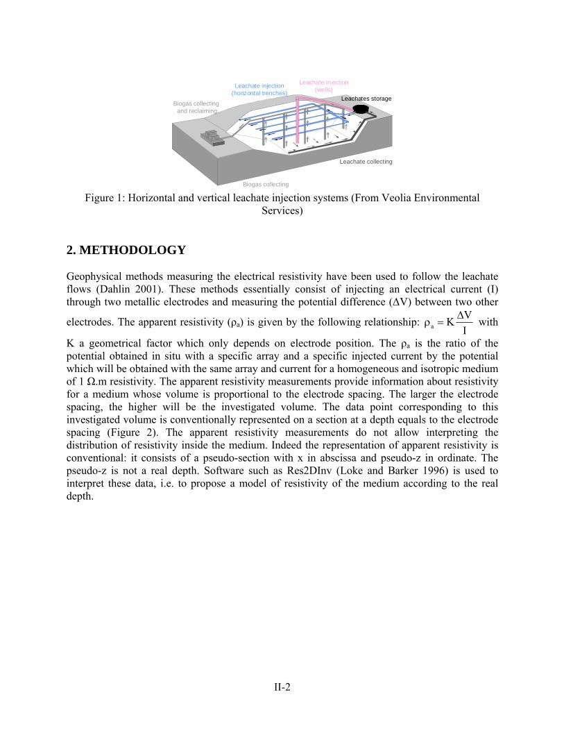
LEACHATE RECIRCULATION 1. INTRODUCTION Recently, the operation of municipal solid waste landfills as bioreactor landfills has gained significant attention of the environmental professionals. The bioreactor landfill concept essentially involves accelerating the waste biodegradation and stabilization process through controlled additions of liquid, often through leachate recirculation, using for example vertical injection wells or horizontal trenches (Figure 1). The increase of moisture content enhances the growth of bacteria responsible of the solid waste decomposition (Warith 2002). The bioreactor landfill allows accelerating the waste biodegradation and decreases the waste stabilization time which limits environmental risks. The biogas production is enhanced during landfill operation, thus it may be easier to use it for energy production. One of the main parameter to ensure acceleration of biodegradation of waste is the waste moisture content. Controlling the quantity and the distribution of leachate injected into the waste mass is essential to optimize the bioreactor landfill performance. Several methods have been developed and implemented to measure the waste moisture content (Imhoff et al. 2007). The most common methods, waste sampling or probe measurements, are intrusive methods and provide data for localized waste. Although the direct method of waste sampling and testing provides accurate waste moisture content, it is difficult and expensive to sample the waste, especially when the landfill is capped. In addition, a large number of waste samples are necessary for accurate determination of moisture distribution because of the waste heterogeneity. The moisture measuring probes such as time domain reflectometry (TDR) probes are commonly used to provide waste moisture. The difficulty with using such probes is the poor contact between probes and waste and also high cost associated with the need for installing several probes to determine spatial distribution of waste moisture. The non-invasive geophysical methods which measure the electrical resistivity, specifically electrical resistivity tomography (ERT), could overcome these problems. Among others, electrical resistivity depends on water content, thus the measured electrical resistivity values allow determination of spatial distribution of waste moisture (not just isolated locations as with probes). Recently, the ERT method has been proved to be efficient to monitor moisture distribution during leachate recirculation in bioreactor landfills in France (Moreau et al. 2003; Rosqvist et al. 2003; Guerin et al. 2004). Nevertheless, no general relationship between electrical resistivity and moisture content is available for MSW. But Grellier (2005) showed that ERT is a suitable method to monitor the leachate recirculation in MSW, and it can provide an estimation of the variations of the moisture content during leachate recirculation events. To date, the ERT method has not been used to monitor moisture distribution in bioreactor landfills in the United States. Because of its proven success in France and distinct advantages over the common methods (sampling or probes), the ERT method has been used to monitor moisture distribution and evaluate the efficiency of leachate recirculation system at Orchard Hills landfill located in Davis Junction, Illinois, USA. This section presents the results of this study.

II-2

Leachate injection

(horizontal trenches)

Biogas collecting

Leachates storageBiogas collecting

and reclaiming

Leachate collecting

Leachate injection(wells)

Figure 1: Horizontal and vertical leachate injection systems (From Veolia Environmental

Services) 2. METHODOLOGY Geophysical methods measuring the electrical resistivity have been used to follow the leachate flows (Dahlin 2001). These methods essentially consist of injecting an electrical current (I) through two metallic electrodes and measuring the potential difference (ΔV) between two other

electrodes. The apparent resistivity (ρa) is given by the following relationship: aVKIΔ

ρ = with

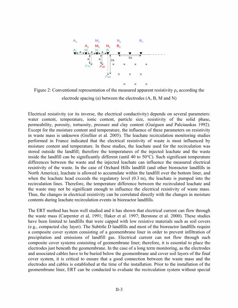
K a geometrical factor which only depends on electrode position. The ρa is the ratio of the potential obtained in situ with a specific array and a specific injected current by the potential which will be obtained with the same array and current for a homogeneous and isotropic medium of 1 Ω.m resistivity. The apparent resistivity measurements provide information about resistivity for a medium whose volume is proportional to the electrode spacing. The larger the electrode spacing, the higher will be the investigated volume. The data point corresponding to this investigated volume is conventionally represented on a section at a depth equals to the electrode spacing (Figure 2). The apparent resistivity measurements do not allow interpreting the distribution of resistivity inside the medium. Indeed the representation of apparent resistivity is conventional: it consists of a pseudo-section with x in abscissa and pseudo-z in ordinate. The pseudo-z is not a real depth. Software such as Res2DInv (Loke and Barker 1996) is used to interpret these data, i.e. to propose a model of resistivity of the medium according to the real depth.

II-3

aA1 B1M1 N1a a

ρa1

a

A3

A2 B2M2 N2

M3 N3 B3

a 2a2a

ρa2

ρa3

Figure 2: Conventional representation of the measured apparent resistivity ρa according the

electrode spacing (a) between the electrodes (A, B, M and N)

Electrical resistivity (or its inverse, the electrical conductivity) depends on several parameters: water content, temperature, ionic content, particle size, resistivity of the solid phase, permeability, porosity, tortuosity, pressure and clay content (Guéguen and Palciauskas 1992). Except for the moisture content and temperature, the influence of these parameters on resistivity in waste mass is unknown (Grellier et al. 2005). The leachate recirculation monitoring studies performed in France indicated that the electrical resistivity of waste is most influenced by moisture content and temperature. In these studies, the leachate used for the recirculation was stored outside the landfill; therefore the temperatures of the injected leachate and the waste inside the landfill can be significantly different (until 40 to 50°C). Such significant temperature differences between the waste and the injected leachate can influence the measured electrical resistivity of the waste. In the case of Orchard Hills landfill (and other bioreactor landfills in North America), leachate is allowed to accumulate within the landfill over the bottom liner, and when the leachate head exceeds the regulatory level (0.3 m), the leachate is pumped into the recirculation lines. Therefore, the temperature difference between the recirculated leachate and the waste may not be significant enough to influence the electrical resistivity of waste mass. Thus, the changes in electrical resistivity can be correlated directly with the changes in moisture contents during leachate recirculation events in bioreactor landfills. The ERT method has been well studied and it has shown that electrical current can flow through the waste mass (Carpenter et al, 1991; Haker et al. 1997; Berstone et al. 2000). These studies have been limited to landfills that were capped with low resistive materials such as soil covers (e.g., compacted clay layer). The Subtitle D landfills and most of the bioreactor landfills require a composite cover system consisting of a geomembrane liner in order to prevent infiltration of precipitation and emissions of landfill gas. Electrical current can not flow through such composite cover systems consisting of geomembrane liner; therefore, it is essential to place the electrodes just beneath the geomembrane. In the case of a long term monitoring, as the electrodes and associated cables have to be buried below the geomembrane and cover soil layers of the final cover system, it is critical to ensure that a good connection between the waste mass and the electrodes and cables is established at the time of the installation. Prior to the installation of the geomembrane liner, ERT can be conducted to evaluate the recirculation system without special

II-4

requirements, and the same equipment can be used on several sites, minimizing the cost of the instrumentation. The ERT method can be implemented with different number of electrodes per line. The use of 48 electrodes per line can result in 684 x 2 measurements for an electrical imaging acquired with the pole-dipole array. Such large number of measurements requires about 2 hours and 15 minutes with a classic resistivity-meter. With such large time requirement, it is not possible to capture the snapshot of moisture distribution at any specified time during leachate recirculation. Therefore, it is important to quickly acquire the data in order not to obtain a biased resistivity distribution. A new generation resistivity-meter, the Syscal Pro designed for high productivity survey by IRIS Instruments, has been used for this study. To reduce time for data acquisition, further optimizations of sequences are required. The above methodology has been validated during monitoring of French bioreactors (Grellier 2005) and is adopted for this study. In order to evaluate the efficiency of the recirculation system, reference electrical resistivity measurements are acquired before the beginning of the recirculation. Then, approximately every 30 minutes, resistivity measurements are made and compared to the reference measurement. The relative differences between measured and reference resistivity values are plotted in order to detect even small resistivity changes linked to the recirculation. As the variations are usually less than 10%, the representation of resistivity does not show clearly the influence of the recirculation. 3. PROJECT SITE The present study is conducted at Orchard Hills Landfill located in Davis Junction, Illinois, USA. The landfill is a large mounded landfill with filling both above- and below-grade. Waste input is approximately 3200 tonnes/day with 70% MSW, 16% C&D, 11% soils and the remainder special waste. The north cell of this landfill is selected for this study. The cell was filled with waste and the leachate recirculation started in September 2005. Leachate recirculation is performed through 6-inch perforated HDPE pipe in gravel-filled trenches, called Leachate Recirculation Lines (LRLs). Figure 3 shows the geophysical lines with respect to the leachate recirculation lines (LRL28 and LRL29) in the north cell. Three horizontal 2D electrical imaging lines (designated as Upstream line, Downstream line, and Alongstream line) are installed, each line consisting of 48 electrodes at a spacing of 2.5 m. The Upstream and Downstream lines are located perpendicular to the leachate recirculation lines (LRL28 and 29) in order to study the lateral spreading of the leachate. Alongstream line is located along the LRL29 in order to study the spreading of leachate along this recirculation line. As shown in Figure 4 and Figure 5, the north cell selected for this study is sloped, and the leachate recirculation lines are as deep as 10 to 15 m from the surface where the geophysical lines are installed.

II-5

Figure 3: Leachate recirculation lines and geophysical instrumentation at the project site

EW

LRL289 m

19m

downstream line upstream line

15.5m12 m

0 20 40 60 80 100 120 140 160 180

distance (m)

230

240

250

elev

atio

n (m

)

topography of the bottom of the cell

9.15 m

Figure 4: Topography of the cell above the leachate recirculation line LRL28

4. FIELD RESULTS Leachate is injected into all leachate recirculation lines sequentially. Generally, leachate is injected for duration of two weeks in each leachate recirculation line. For the north cell, the leachate recirculation is sequenced among the five leachate recirculation lines (LRL28, LRL29 and three other deeper leachate recirculation lines shown in thin orange dashed lines in Figure 3). This means that leachate is recirculated on the same LRL every 10 weeks. The leachate is stored in the sump at the bottom of the cell and four pumps are automatically activated when the leachate level exceeds regulatory limit of 30 cm above the bottom liner. Flowmeters are installed at each injection locations to measure the quantity of leachate recirculated into the LRLs. Unlike the controlled leachate recirculation events at French bioreactor landfills, the leachate recirculation operations at the Orchard Hills landfill are dependent up on the amount of leachate produced and also on the planned sequential injection into different recirculation lines. Several

II-6

series of geophysical measurements are being made to optimize the flow rate and duration of recirculation in LRL28 and LRL29 in order to detect the recirculation effects on ERTs.

EW7.6 m

13.6mdownstream line

upstream line

11.7m

0 20 40 60 80 100 120 140 160 180 200

distance (m)

220

230

240

250

elev

atio

n (m

)


10.3 m

LRL29

alongstream line

Figure 5: Topography of the cell above the leachate recirculation line LRL29

Initial geophysical measurements are made prior to leachate injection to establish the reference electrical resistivity distribution in the study area. Then, the leachate is injected into the LRL29 at the average flow rate of 3 m3/h. The total quantity of recirculated leachate during the geophysical measurements period is 17.8 m3. Geophysical measurements are made Alongstream and Upstream at different time periods during leachate recirculation. Figure 6 and Figure 7 present the monitoring of resistivity during the leachate recirculation into LRL29 on Alongstream line and Upstream line. The first cross-section in each figure is an interpreted resistivity (ρref) section obtained before the beginning of the leachate injection and used as reference (in black and white). The following cross-sections show the relative variation of interpreted resistivity (in color) calculated with the formula: 100.(ρi-ρref)/ρref, with ρi the interpreted resistivity at the time i. Decreasing resistivity appears in green-blue on the map (negative variations), and increasing appears in orange-red (positive variations). The leachate is injected from the east end of the LRL29. As seen in Figure 6, the resistivity is decreasing compared to the reference, especially near the injection entry of the LRL29 (on the east end of the LRL). Along the last 20 m of the LRL, the resistivity is neither decreasing nor increasing. This implies that the injected leachate does not reach the end of the LRL. The resistivity variations in the bottom or sides of the cross-sections (Figure 6) are difficult to interpret as they may be due to artifacts or side effects. Figure 7 shows resistivity variations perpendicular to the LRL29. A plume of negative resistivity variations is observed around the LRL during the leachate injection. In this case, the resistivity variations are correlated to the leachate injection. Based on these initial results, the zone of influence of the LRL could be estimated at around 30 m. Even if this is the same order of magnitude as the one determined for French bioreactors with a horizontal recirculation system (Grellier et al. 2005; Moreau et al. 2003), these results need to be confirmed. The propagation of the plume around LRL29 is following the slope of the cell. The compaction of the waste during the landfilling is generally in the horizontal direction; therefore preferential pathways are not expected in the direction of the slope. High resistivity variations are observed on the south side of the sections where no recirculation of leachate occurs. Additional geophysical measurements are needed to confirm these results and to determine the causes for the observed results. Additional geophysical measurements are also needed to determine the zone of influence under a higher flow and greater leachate quantity than those used for this study.

II-7

220

230

240

250

12 16 20 27 35 46 60 78 102 134

6-ref

-4

-3

-2

-1

-0

0

1

2

3

4

220

230

240

250

220

230

240

250

0 20 40 60 80 100 120distance (m)

220

230

240

250

elev

atio

n (m

)6-5 - 6-ref

6-6 - 6-ref

6-7 - 6-ref

1h07 during recirculation



E W

ρ (Ω.m)

%

LRL29 Figure 6: Variation of resistivity on alongstream line during leachate recirculation on LRL29.

5. CONCLUSIONS The electrical resistivity tomography methodology developed in France for the monitoring of leachate recirculation has been adopted to monitor leachate recirculation at Orchard Hills landfill located in Davis Junction, Illinois, USA. The leachate recirculation in the north cell of this landfill is monitored through three horizontal 2D electrical imaging lines with each line consisting of 48 electrodes at a spacing of 2.5 m. A new generation resistivity-meter is used to make fast measurements so that the evolution of moisture content and zone of influence can be captured for the selected short-duration leachate recirculation event. The monitoring results helped to assess the moisture distribution along and perpendicular of the leachate recirculation lines. Although the leachate distribution along the leachate recirculation lines is not clearly evident, the leachate distribution around the recirculation line shows a decrease of resistivity around the line. The initial estimation of the influence zone is similar to the ones observed at French bioreactor landfills, but additional measurements are needed to confirm it. Even though, more comprehensive monitoring is needed, the results of this study show that ERT method has a great potential to be used as monitoring tool to optimize the leachate recirculation, leading to the best performance of bioreactor landfills.

II-8

220

230

240

250

12

16

20

27

35

46

60

78

102

1346-ref

220

230

240

250

-13

-10

-7

-4

-1

1

4

7

10

13

220

230

240

250

220

230

240

250

220

230

240

250

6-8 - 6-ref

6-9 - 6-ref

6-10 - 6-ref

6-11 - 6-ref

5min after 10min of recirculation

1h36 after 10min of recircualtion

9min during recirculation

45min during recircualtion

S N

ρ (Ω.m)

%

220

230

240

250 6-12 - 6-ref

2h41 during recircualtion

10 20 30 40 50 60 70 80 90 100 110distance (m)

220

230

240

250

elev

atio

n (m

)

6-13 - 6-ref

4h41 during recircualtion

LRL 28LRL 29

D

Figure 7: Variation of resistivity on upstream line during leachate recirculation on LRL29.

Additional geophysical monitoring is needed under high leachate injection flow rate and greater quantity to delineate the evolution of moisture and zone of influence. In addition to the electrical imaging, a drilling program has been implemented in this study area. Waste samples from different depths have been collected and tested for moisture content. These results are used to validate the accuracy of the electrical imaging results (see section III).

II-9

CITED REFERENCES Bernstone, C., Dahlin, T., Ohlsson, T., and Hogland, W., 2000, “DC-resistivity mapping of

internal landfill structures: two pre-excavation surveys”, Environmental Geology, 39 (3-4), 360-371.

Carpenter, P.J., Calkin, S.F., and Kaufmann, R.S., 1991, “Assessing a fractured landfill cover using electrical resistivity and seismic refraction techniques”, Geophysics, 56, 11, 1896-1904.

Dahlin, T., 2001, “The development of DC resistivity imaging techniques”, Computers & Geosciences, 27 (9), 1019-1029.

Grellier S., 2005, “Suivi hydrologique des centres de stockage de déchet-bioréacteurs par mesures géophysiques”, PhD thesis, Université Pierre et Marie Curie, Paris, 238 p.

Grellier, S., Bouyé, J.M., Guérin, R., Robain, H., and Skhiri, N., 2005, “Electrical Resistivity Tomography (ERT) applied to moisture measurements in bioreactor: principles, in situ measurements and results”, International Workshop “Hydro-Physico-Mechanics of Landfills”, Grenoble (France), 21-22 March.

Guéguen Y., and Palciauskas V., 1992, “Introduction à la physique des roches”, Hermann, éditeurs des sciences et des arts, 299 p.

Guérin, R., Munoz, M.L., Aran, C., Laperrelle, C., Hidra, M., Drouart, E., and Grellier, S, 2004, “Leachate recirculation: moisture content assessment by means of a geophysical technique”. Waste Management, 24 (8), 785-794

Haker, C.D., Rix, G.J., and Lai, C.G., 1997, “Dynamic properties of municipal solid waste landfills from surface wave tests”, Proc SAGEEP’97 (Symposium on the Application of Geophysics to Engineering and Environmental Problems), Environmental and Engineering Geophysical Society, Wheat Ridge (USA), 301-310.

Imhoff, P.T., Reinhart, D.R., Englund, M., Gurin, R., Gawande, N., Han, B., Jonnalagadda, S., Townsend, T., and R. Yazdani, 2007, “Methods for measuring liquid in bioreactor landfills - A critical review”. Waste Management, 27:729-745.

Loke, M.H., and Barker, R.D., 1996, “Rapid least-square inversion of apparent resistivity pseudosections by a quasi-Newton method”, Geophysical Prospecting, 44 (2), 131-152.

Moreau, S., Bouyé, J.M., Barina, G., and Oberti, O., 2003, “Electrical resistivity survey to investigate the influence of leachate recirculation in a MSW landfill”, Proceedings of the 9th International Waste Management and Landfill Symposium, Session C02, CISA publ.

Rosqvist, H., Dahlin, T., Fourie, A., Röhrs, L., Bengtsson, A., and Larsson, M., 2003, “Mapping of leachate plumes at two landfill sites in South Africa using geoelectrical imaging techniques”, Proceedings of the 9th International Waste Management and Landfill Symposium, Session C02, CISA publ.

Warith, M., 2002, “Bioreactor landfills: experimental and field results”, Waste Management, 22 (1), 7-17.

III-1

SECTION III CORRELATION BETWEEN ELECTRICAL RESISTIVITY AND

MOISTURE CONTENT OF MSW

1. INTRODUCTION Electrical resistivity tomography (ERT) has been used to monitor leachate recirculation in bioreactor landfills in France on the basis of decreasing resistivity values in the waste around the recirculation system during leachate recirculation events (Guerin 2004; Moreau 2003). However, direct correlation between the resistivity and the moisture content is not established because of the dependence of the resistivity on several other parameters such as temperature, ionic content, particle size, resistivity of the solid phase, permeability, porosity, tortuosity, pressure, and clay content (Guéguen and Palciauskas 1992). Based on a large-scale laboratory testing program, Grellier et al. (2005) developed relationships between electrical resistivity and temperature and between electrical resistivity and water content of MSW assuming that the waste does not degrade within the short duration of the testing period. As of today, a direct correlation between the in-situ measured electrical resistivity and the moisture content of the waste has not been reported (Imhoff et al. 2007). Such a relationship will be valuable to evaluate the moisture content evolution with ERT during leachate recirculation events in landfills. This section presents the results of a field study aimed to: (1) correlate the electrical resistivity measured by ERT with the waste moisture content, and (2) study the influence of the leachate recirculation on the waste moisture content at different depths and different distances from the leachate recirculation lines based on characterization of waste samples and ERT results. Electrical resistivity tomography is performed at three locations of Orchard Hills landfill to determine the electrical resistivity with depth at these locations. Immediately after the ERT measurements, boreholes are drilled at each location to collect the waste samples at different depths to determine moisture content in the laboratory. The one-to-one comparison of electrical resistivity and moisture content profiles at the locations allowed investigation of direct correlation between the electrical resistivity and the moisture content of waste. This correlation is then applied to estimate the spatial moisture content distribution using the measured electrical resistivity distributions at three locations of the landfill to investigate the influence of leachate recirculation system on the evolution of moisture content of waste. 2. FIELD TESTING 2.1 Electrical Resistivity Tomography As explained in section II, the ERT consists of injecting an electrical current (I) through two metallic electrodes and measuring the potential difference (ΔV) between two other electrodes (Dahlin 2001). The apparent resistivity (ρa) is given by the following relationship:

aVKIΔ

ρ = (Equation 1)

III-2

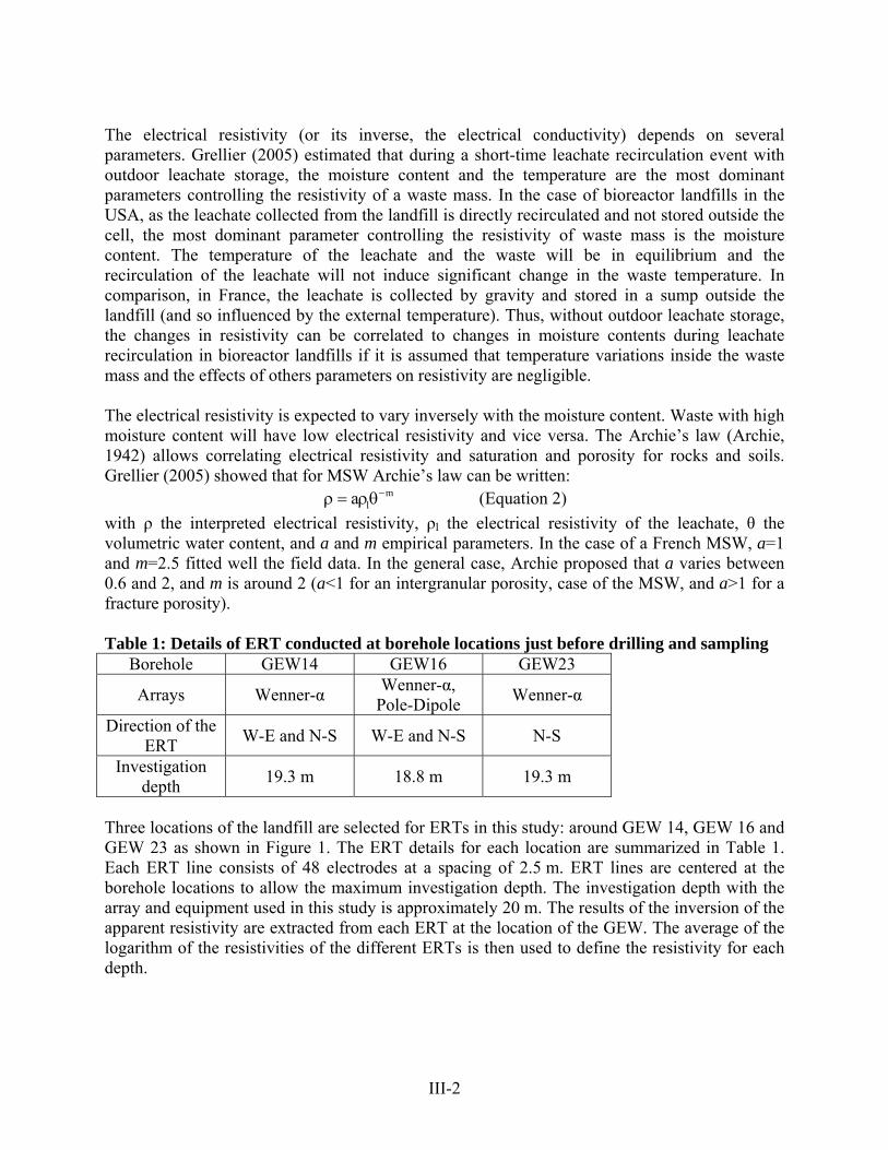
The electrical resistivity (or its inverse, the electrical conductivity) depends on several parameters. Grellier (2005) estimated that during a short-time leachate recirculation event with outdoor leachate storage, the moisture content and the temperature are the most dominant parameters controlling the resistivity of a waste mass. In the case of bioreactor landfills in the USA, as the leachate collected from the landfill is directly recirculated and not stored outside the cell, the most dominant parameter controlling the resistivity of waste mass is the moisture content. The temperature of the leachate and the waste will be in equilibrium and the recirculation of the leachate will not induce significant change in the waste temperature. In comparison, in France, the leachate is collected by gravity and stored in a sump outside the landfill (and so influenced by the external temperature). Thus, without outdoor leachate storage, the changes in resistivity can be correlated to changes in moisture contents during leachate recirculation in bioreactor landfills if it is assumed that temperature variations inside the waste mass and the effects of others parameters on resistivity are negligible. The electrical resistivity is expected to vary inversely with the moisture content. Waste with high moisture content will have low electrical resistivity and vice versa. The Archie’s law (Archie, 1942) allows correlating electrical resistivity and saturation and porosity for rocks and soils. Grellier (2005) showed that for MSW Archie’s law can be written:

mla −ρ = ρθ (Equation 2)

with ρ the interpreted electrical resistivity, ρl the electrical resistivity of the leachate, θ the volumetric water content, and a and m empirical parameters. In the case of a French MSW, a=1 and m=2.5 fitted well the field data. In the general case, Archie proposed that a varies between 0.6 and 2, and m is around 2 (a<1 for an intergranular porosity, case of the MSW, and a>1 for a fracture porosity). Table 1: Details of ERT conducted at borehole locations just before drilling and sampling

Borehole GEW14 GEW16 GEW23

Arrays Wenner-α Wenner-α, Pole-Dipole Wenner-α

Direction of the ERT W-E and N-S W-E and N-S N-S

Investigation depth 19.3 m 18.8 m 19.3 m

Three locations of the landfill are selected for ERTs in this study: around GEW 14, GEW 16 and GEW 23 as shown in Figure 1. The ERT details for each location are summarized in Table 1. Each ERT line consists of 48 electrodes at a spacing of 2.5 m. ERT lines are centered at the borehole locations to allow the maximum investigation depth. The investigation depth with the array and equipment used in this study is approximately 20 m. The results of the inversion of the apparent resistivity are extracted from each ERT at the location of the GEW. The average of the logarithm of the resistivities of the different ERTs is then used to define the resistivity for each depth.

III-3

Figure 1: Map of the studied landfill cell showing three borehole locations and position of ERTs 2.2 Waste Sampling and Testing Immediately following the ERTs, boreholes are drilled at the three locations using bucket auguring method. The drilling is performed in conjunction with the installation of gas extraction wells at these locations. The depth of each borehole and the number of waste samples collected at each location are summarized in Table 2, and the distances between the borehole locations and the closest leachate recirculation lines are also shown in this table. Borehole locations GEW14 and GEW16 are selected within the leachate recirculation areas of the landfill cell to study the influence of leachate recirculation on moisture content of waste. Waste in borehole GEW14 should be affected by the leachate recirculation lines LRL18 and LRL19 (deep lines), and the waste in borehole GEW16 should be affected by LRL29 (shallow line) and LRL26 (deep line). Borehole GEW23 is situated farther away from the recirculation lines; therefore, it will serve as reference location where the waste is not influenced by the leachate recirculation (representing conventional landfill conditions). During the drilling, waste samples, each weighing approximately 30 kg, are collected at every 3 m depth up to the termination of the boreholes. Temperature of the waste samples is measured immediately upon the retrieval to the ground surface. The waste samples are weighed in the field and then sealed in plastic bags. The samples are then transported to the laboratory for moisture content testing. The moisture content of waste samples is determined by drying in ovens at 60°C

III-4

for several days (until there is no change in total mass). Based on the results, the wet gravimetric moisture content (ww) is calculated by:

lw

tw

MwM

= (Equation 3)

with Ml the mass of liquid in the sample, and Mtw the mass of the total wet sample. Usually, the electrical resistivity is related to volumetric moisture content (θ) which is defined by:

l

tw

VV

θ = (Equation 4)

with Vl the volume of liquid and Vtw the volume of the total wet sample. The gravimetric moisture content and volumetric water content are related by the following relationship:

lw

tw

DwD

= θ (Equation 5)

with Dl the density of the liquid which approximately equals to 1,000 kg/m3 and Dtw the bulk (total) density of the wet sample. Table 2: Details of drilling and sampling at three borehole locations

Borehole GEW14 GEW16 GEW23 Depth 31 m 28.8 m 11.2 m

Samples 11 12 5

Distance from the

closest LRL

26.5 m from the LRL189.8 m from the LRL19

7.5 m from the LRL29 11.9 m from the LRL26

68 m from the LRL16 88 m from the LRL17 75 m from the LRL18 51 m from the LRL19 87 m from the LRL23 75 m from the LRL24

3. RESULTS AND ANALYSIS The resistivity values of the waste samples from the boreholes are corrected for temperature based on the waste temperature data recorded every 1.5 m during the drilling using the relationship determined by Grellier et al. (2006). This relationship indicates that the electrical resistivity decreases by about 2% for temperature increase of 1°C. Waste temperatures range from 20 to 38°C, from 3 m depth to the bottom of the boreholes. At 1.5 m from the surface, lower temperatures are measured (from 5 to 14°C). Equation 5 is used to convert the measured gravimetric moisture contents into volumetric moisture content or vice-versa. For this conversion, the density of the waste must be known. Based on the total mass of waste disposed in the landfill cell divided by the total volume of the cell, the average wet density of waste is determined to be 890 kg/m3. In addition, the wet density of waste at different depths is measured during drilling a borehole numbered GEW10 within the landfill cell by measuring the volume of borehole depth zone and the waste mass recovered from it. Based on this, the average density of waste is determined to be 1,500 kg/m3, with values ranging from 1,220 to 2,000 kg/m3. This range of density values and the global average value are used for the conversion of the moisture content of the waste.

III-5

3.1 Correlation between Resistivity and Wet Gravimetric Moisture Content Figure 2 presents the measured electrical resistivity (ρ) and wet gravimetric moisture content (ww) versus depth at each borehole location (GEW). At location GEW14 (Figure 2a), the moisture content increases within the elevation interval of 253 m and 238 m, and then it decreases. In the same elevation range, the resistivity starts to decrease and then it increases. The inverse relationship between electrical resistivity and moisture is evident from these results. At location GEW16 (Figure 2b), moisture content is low close to the surface, then it increases to an elevation of 230 m, and finally shows decreasing trend at the bottom of the borehole. The decrease in resistivity with increase in moisture is also observed at this location. The trend for the moisture content of the waste samples at location GEW23 is less obvious as there are only few data points (Figure 2c). A general trend of slightly increase of the moisture with the depth is observed. This is correlated with the slight decrease of resistivity with depth. The fluctuating moisture content values observed at all three locations are mainly as a result of heterogeneous nature of the waste and the use of a small representative waste sample for laboratory moisture content testing. Therefore, instead of point-to-point correlation, a general correlation between moisture content and resistivity is observed at the three borehole locations as seen in Figure 2(d).

10 20 30 40 50

Wet Moisture Content ww%Electrical Resistivity ρ (Ω.m)

220

230

240

250

260

Elev

atio

n (m

)

measured ww

ρww calculated

from Archie's law

0.1 1 10 100

GEW 14

10 20 30 40 50

Wet Moisture Content ww %Electrical Resistivity ρ (Ω.m)

220

230

240

250

260

Elev

atio

n (m

)

measured ww

ρww calculated from Archie's law

0.1 1 10 100

GEW 16

a) Borehole GEW 14 b) Borehole GEW 16

III-6

10 20 30 40 50

Wet Moisture Content ww %Electrical Resistivity ρ (Ω.m)

224

228

232

236

240El

evat

ion

(m)

measured ww

ρww calculated from Archie's law

0.1 1 10 100

GEW 23

10 20 30 40 50

Wet Moisture Content %Electrical Resistivity (Ω.m)

220

230

240

250

260

Elev

atio

n (m

)

ww GEW14ww GEW16ww GEW23

ρ GEW14ρ GEW16ρ GEW23

0.1 1 10 100

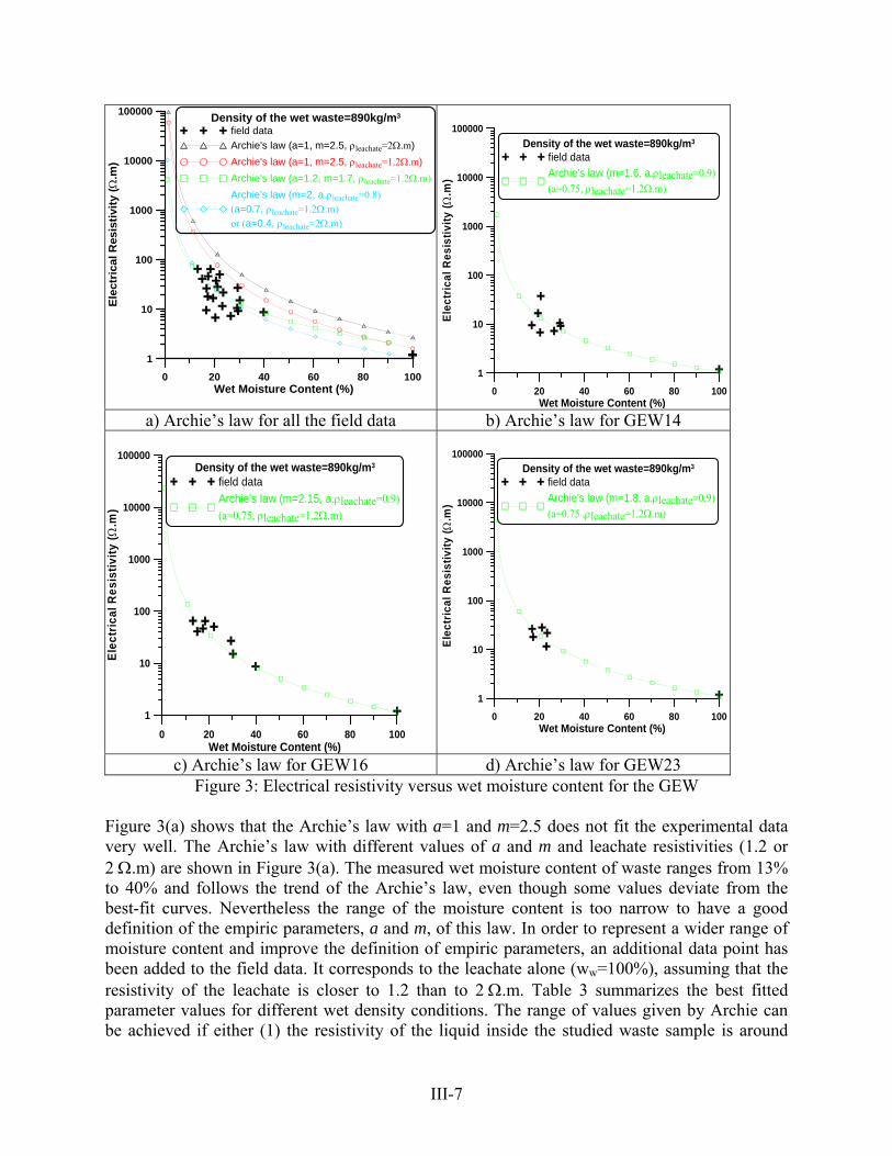
c) Borehole GEW 23 d) Data for Three Borehole Locations Figure 2: Wet gravimetric moisture content ww (%) and electrical resistivity ρ (Ω.m) versus elevation (depth) at three borehole (GEW) locations To correlate electrical resistivity with wet gravimetric moisture content, the volumetric water content in the Archie’s law is converted into wet gravimetric water content using density of waste according to Equation 3. The correlations have been evaluated for different wet densities of waste ranging from 890 kg/m3 to 1,500 kg/m3. Figure 3 represents the electrical resistivity of the waste versus the moisture content of the drilled samples for the three studied borehole locations (GEW) using the average wet waste density of 890 kg/m3. The electrical resistivity and wet gravimetric moisture content data in Figure 3 is fitted with Archie’s law as given in Equation 2. In this equation, ρl is the leachate conductivity. At Orchard Hills landfill, the electrical conductivity of leachate is measured quarterly in four leachate collection points. The average leachate conductivity is around 5,000 mS/cm (or electrical resistivity of 2 Ω.m), between February 2004 and November 2005, but increased to 8,000 mS/cm (or electrical resistivity of 1.2 Ω.m) in February 2006. These two values are selected for the evaluation of correlation between electrical resistivity and moisture content using Archie’s law. The electrical resistivity range of the waste is about 5 to 100 Ω.m. These values are comparable to typical values of clay or wet sand. The maximum resistivities for dry soils and rocks can be in the order of few thousand Ω.m.

III-7

0 20 40 60 80 100Wet Moisture Content (%)

1

10

100

1000

10000

100000El

ectr

ical

Res

istiv

ity (Ω

.m)

Density of the wet waste=890kg/m3

field dataArchie's law (a=1, m=2.5, ρleachate=2Ω.m)Archie's law (a=1, m=2.5, ρleachate=1.2Ω.m)Archie's law (a=1.2, m=1.7, ρleachate=1.2Ω.m)Archie's law (m=2, a.ρleachate=0.8)(a=0.7, ρleachate=1.2Ω.m) or (a=0.4, ρleachate=2Ω.m)


1

10

100

1000

10000

100000

Elec

tric

al R

esis

tivity

(Ω.m

)


field dataArchie's law (m=1.6, a.ρleachate=0.9)(a=0.75, ρleachate=1.2Ω.m)

a) Archie’s law for all the field data b) Archie’s law for GEW14


1

10

100

1000

10000

100000

Elec

tric

al R

esis

tivity

(Ω.m

)


field dataArchie's law (m=2.15, a.ρleachate=0.9)(a=0.75, ρleachate=1.2Ω.m)


1

10

100

1000

10000

100000El

ectr

ical

Res

istiv

ity (Ω

.m)


field dataArchie's law (m=1.8, a.ρleachate=0.9)(a=0.75 ,ρleachate=1.2Ω.m)

c) Archie’s law for GEW16 d) Archie’s law for GEW23 Figure 3: Electrical resistivity versus wet moisture content for the GEW

Figure 3(a) shows that the Archie’s law with a=1 and m=2.5 does not fit the experimental data very well. The Archie’s law with different values of a and m and leachate resistivities (1.2 or 2 Ω.m) are shown in Figure 3(a). The measured wet moisture content of waste ranges from 13% to 40% and follows the trend of the Archie’s law, even though some values deviate from the best-fit curves. Nevertheless the range of the moisture content is too narrow to have a good definition of the empiric parameters, a and m, of this law. In order to represent a wider range of moisture content and improve the definition of empiric parameters, an additional data point has been added to the field data. It corresponds to the leachate alone (ww=100%), assuming that the resistivity of the leachate is closer to 1.2 than to 2 Ω.m. Table 3 summarizes the best fitted parameter values for different wet density conditions. The range of values given by Archie can be achieved if either (1) the resistivity of the liquid inside the studied waste sample is around

III-8

1.2 Ω.m and the density of the waste is around 890 kg/m3 or (2) the resistivity of the liquid inside the studied waste sample is around 2 Ω.m and the density of the waste is around 1,200 kg/m3. Table 3: Best-fit a and m parameters from the Archie’s law based on the field data Field Data Points and Wet Waste Density (D)

ρleachate=1.2 Ω.m ρleachate=2 Ω.m

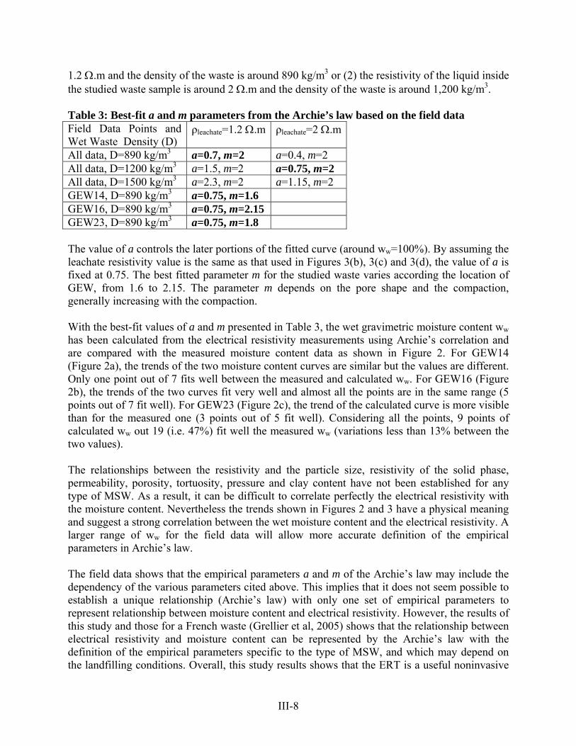
All data, D=890 kg/m3 a=0.7, m=2 a=0.4, m=2 All data, D=1200 kg/m3 a=1.5, m=2 a=0.75, m=2 All data, D=1500 kg/m3 a=2.3, m=2 a=1.15, m=2 GEW14, D=890 kg/m3 a=0.75, m=1.6 GEW16, D=890 kg/m3 a=0.75, m=2.15 GEW23, D=890 kg/m3 a=0.75, m=1.8 The value of a controls the later portions of the fitted curve (around ww=100%). By assuming the leachate resistivity value is the same as that used in Figures 3(b), 3(c) and 3(d), the value of a is fixed at 0.75. The best fitted parameter m for the studied waste varies according the location of GEW, from 1.6 to 2.15. The parameter m depends on the pore shape and the compaction, generally increasing with the compaction. With the best-fit values of a and m presented in Table 3, the wet gravimetric moisture content ww has been calculated from the electrical resistivity measurements using Archie’s correlation and are compared with the measured moisture content data as shown in Figure 2. For GEW14 (Figure 2a), the trends of the two moisture content curves are similar but the values are different. Only one point out of 7 fits well between the measured and calculated ww. For GEW16 (Figure 2b), the trends of the two curves fit very well and almost all the points are in the same range (5 points out of 7 fit well). For GEW23 (Figure 2c), the trend of the calculated curve is more visible than for the measured one (3 points out of 5 fit well). Considering all the points, 9 points of calculated ww out 19 (i.e. 47%) fit well the measured ww (variations less than 13% between the two values). The relationships between the resistivity and the particle size, resistivity of the solid phase, permeability, porosity, tortuosity, pressure and clay content have not been established for any type of MSW. As a result, it can be difficult to correlate perfectly the electrical resistivity with the moisture content. Nevertheless the trends shown in Figures 2 and 3 have a physical meaning and suggest a strong correlation between the wet moisture content and the electrical resistivity. A larger range of ww for the field data will allow more accurate definition of the empirical parameters in Archie’s law. The field data shows that the empirical parameters a and m of the Archie’s law may include the dependency of the various parameters cited above. This implies that it does not seem possible to establish a unique relationship (Archie’s law) with only one set of empirical parameters to represent relationship between moisture content and electrical resistivity. However, the results of this study and those for a French waste (Grellier et al, 2005) shows that the relationship between electrical resistivity and moisture content can be represented by the Archie’s law with the definition of the empirical parameters specific to the type of MSW, and which may depend on the landfilling conditions. Overall, this study results shows that the ERT is a useful noninvasive

III-9

technique to evaluate the moisture content. Similar to all the other invasive and noninvasive non-direct methods, a calibration between the measured properties and the moisture content is needed. For the bioreactor landfills, such a calibration may be required at different degradation states of the waste (due to changes in particle size, porosity, etc.). 3.2 Influence of Leachate Recirculation on Evolution of Wet Moisture Content Figures 4, 5 and 6 present the spatial variation of in-situ measured electrical resistivity and the wet moisture content calculated with the Archie’s law from the electrical resistivity around each borehole location (GEW). The calculation of the wet moisture content with the Archie’s law assumes that the empirical parameters a and m and density of waste are the same along the ERT lines and that the temperature changes are too small to influence the electrical resistivity. The measured (actual) wet moisture contents of the waste samples collected from different depths in boreholes (GEW) are plotted on the moisture content distribution map for comparison purposes, as well as the locations of the closest LRLs. Contrary to the direct wet moisture content measurement, ERT is a global measurement method that does not yield sudden changes in electrical resistivity (hence the moisture content determined using the Archie’s law) within a short distance. Figure 4(a) shows that the measured electrical resistivity at and around borehole location GEW14 generally decreases with depth and then somewhat remains uniform and low up to the depth of investigation (about 20 m). The resistivity is converted into wet moisture content using the Archie’s law as summarized in Figure 4(b), and these results show the inverse relationship between moisture content and resistivity. The moisture content increases with depth and a somewhat higher moisture zone exists between the elevations 250 m and 240 m with moisture content ranging from 20% to 30%. This is consistent with the measured moisture content values for the waste samples (from 20 to 27%). For the top half of the borehole, the actual moisture content values ww is increasing (from 17-19% to 30%). Then in the bottom half of the borehole, ww is decreasing (from 30 to 20%). The average wet moisture content for all the collected samples of GEW14 is 21.7%. The two closest LRLs to GEW14 are deep lines oriented in east-west direction as shown in Figure 4. The presence of the LRL 19 (located at 9.8 m from the GEW14) does not seem to affect the moisture distribution. The LRL18 seems too far (26.5 m) from the borehole location to influence the moisture content of the waste. The observed moisture content variations at shallow depths are attributed to the surface application of leachate during filling operations and potential infiltration of precipitation (this location was not capped during the time of this field investigation). Between the beginning of the recirculation and the drilling of boreholes, 218 and 232 m3 of leachate are recirculated through LRL18 and 19, respectively. This leads to a recirculation rate of 1.1 L and 0.8 L of leachate per ton of waste, respectively, assuming that the average density of the waste of 890 kg/m3, radius of influence of 10 m, and a homogeneous distribution of the leachate all along the lengths of the line. Thus, the leachate injected into LRL19 or 18 may be low and/or the zone of influence of these LRLs is less than 10 m.

III-10

10 20 30 40 50 60 70 80 90 100 110Distance (m)

230

240

250

Ele

vatio

n (m

)

LRL18 LRL19 ρ

5 10 15 20 25 30 35 40 45 50 55 60 65 70 75 80 85 90 95 100 105 110Distance (m)

225

230

235

240

245

250

Elev

atio

n (m

)

19% 17%

27% 20% 30% 29%

21% 23% 21% 20% 14%

wet moisture content

16253342515968778594

791114161921242628

ρ (Ω.m)

%SN

LRL19 LRL18

SN

GEW14

GEW14

(a)

(b)

Figure 4: Electrical resistivity ρ (figure (a)) and wet moisture content (figure (b)) calculated with the Archie’s law from the electrical resistivity around borehole GEW14. The wet moisture contents of the collected waste samples are indicated.

10 20 30 40 50 60 70 80 90 100 110Distance (m)

230

240

250

Elev

atio

n (m

)

LRL29

LRL26ρ

5 10 15 20 25 30 35 40 45 50 55 60 65 70 75 80 85 90 95 100 105 110Distance (m)

225

230

235

240

245

250

Elev

atio

n (m

)

15% 22% 13% 18% 17%

29% 30% 40% 26% 25% 27% 19%


16253342515968778594

791114161921242628

ρ (Ω.m)

%NS

LRL29

LRL26

NS

GEW16

GEW16

(a)

(b)

Figure 5: Electrical resistivity ρ (figure (a)) and wet moisture content (figure (b)) calculated with the Archie’s law from the electrical resistivity around borehole GEW16. The wet moisture contents of the collected waste samples are indicated. Figure 5 shows the variation of the electrical resistivity and interpreted wet moisture content around the borehole location GEW16. The interpreted moisture contents at different depths at the borehole location fit well with the actual measured water content values of the samples collected in the borehole. The average wet moisture content for all the collected samples of GEW16 is

III-11

23.6%. The two closest LRLs to the borehole location are LRL29 and LRL26 as shown in Figure 5. At the depth of the LRL 29 (located at 7.5 m from the GEW16), the wet moisture content is higher (18 and 17.5%) than just above the LRL29 (13%). With increasing depth, the wet moisture content increases (from about 18% at the depth of the LRL29 until 40% 10 m below the LRL29). Therefore, it can be concluded that the leachate recirculation on LRL29 has increased the moisture content of the waste below the LRL by 208% (from 13% to 40%). The wet moisture content of the samples is decreased from 40% to 20% at deeper depths to the bottom of the GEW. It seems that LRL26 may not have significantly affected the moisture content of the waste. The interpreted moisture content distribution is not uniform around the borehole location (Figure 5b). With the shallow LRL29 located on the south side of GEW16, it can be clearly seen that higher wet moisture contents exist in this area than the north side where only the deep LRL26 is present. The last leachate recirculation occurred on LRL29 about 12 days before the drilling of the borehole. The leachate should have had time to drain through the waste. This can explain the higher moisture content at the bottom of the GEW rather than around the LRL29. Overall, these results show that the radius of influence of recirculation is greater than 8 m, but less than 12 m. Between the beginning of the recirculation and the drillings, 531 and 609 m3 of leachate are recirculated through LRL26 and 29, respectively. This leads to a recirculation rate of 79.2 L of leachate per ton of waste respectively with the average density of the waste of 890 kg/m3, radius of influence of 10 m, and a homogeneous distribution of the leachate all along the lengths of the line.

-20 -10 0 10 20 30 40 50 60 70 80 90 100 110 120 130Distance (m)

225

230

235

Elev

atio

n (m

)

LRL16 LRL18LRL19

ρ

-20 -10 0 10 20 30 40 50 60 70 80 90 100 110 120 130Distance (m)

225

230

235

Elev

atio

n (m

) 21%

17% 24% 17%

23%

LRL16 LRL17 LRL19


16253342515968778594

791114161921242628

ρ (Ω.m)

%NS

NS

GEW23

GEW23

LRL23

(a)

(b)

LRL17

Figure 6: Electrical resistivity ρ (figure (a)) and wet moisture content (figure (b)) calculated with the Archie’s law from the electrical resistivity around borehole GEW23. The wet moisture contents of the collected waste samples are indicated. Figure 6 shows measured resistivity and interpreted wet moisture content distribution at and around the borehole location GEW23. The LRLs in the vicinity of the borehole are oriented in the east-west direction. Compared to GEW14 and 16, all the LRL are farther than 50 m from the borehole. The actual moisture contents of the waste samples collected at different depths in the

III-12

borehole are plotted. The average wet moisture content for all the collected samples of GEW23 is 20.4%. The inverse correlation between the electrical resistivity and moisture content is clearly seen for the results. The wet moisture content distribution shows a global increase of moisture content with depth. The results from the three borehole locations show that the moisture content distribution plots obtained by applying the Archie’s law to the measured electrical resistivity using ERT can provide an understanding of the moisture distribution and zone of influence and will help towards optimization of the leachate recirculation operations at bioreactor landfills. 4. CONCLUSIONS Three boreholes are drilled through the waste in Orchard Hills landfill that allowed correlating the electrical resistivity measured before the drilling and the wet gravimetric moisture content measured using waste samples obtained during the drilling. This study shows that the Archie’s law describes well the relationship between electrical resistivity and the wet moisture content. The two empirical parameters of this law have been defined for each borehole and allowed calculating the wet moisture content from the electrical resistivity. The calculated moisture content data fitted reasonably well with the measured data. Therefore, the ERT method seems very promising to assess moisture distribution in waste. The difficulty to apply it routinely is the necessity to calibrate the empirical parameters for each new MSW or each stage of the biodegradation, considering that even in the same landfill cell the parameters can vary. The study of the wet moisture content from collected samples regarding the location of the samples from the LRL shows that the zone of influence of the recirculation system is greater than 8 m but less than 10 m as the two LRLs at 10 and 12 m from the samples do not seem to have an influence on the moisture content of the waste. The average wet moisture content of the GEW16, which is the closest borehole to the LRLs, is 9% and 15% higher than for GEW14 and GEW23, respectively. CITED REFERENCES Archie, G.E. (1942). “The electrical resistivity log as an aid in determining some reservoir

characteristics.” Transactions American Institute of Mining Metallurgical and Petroleum Engineers, 146, 54-67.

Dahlin, T. (2001). “The development of DC resistivity imaging techniques.” Computers & Geosciences, 27 (9), 1019-1029.

Guéguen, Y., and Palciauskas, V. (1992). “Introduction à la physique des roches.” Hermann, éditeurs des sciences et des arts.

Grellier, S. (2005). “Suivi hydrologique des centres de stockage de déchet - bioréacteurs par mesures géophysiques.” Thèse de doctorat, Université Pierre et Marie Curie.

III-13

Grellier, S., Robain, H., Bellier, G., and Skhiri N. (2006). “Influence of temperature on the electrical conductivity of leachate from Municipal Solid Waste.” Journal of Hazardous Materials, in press.

Grellier, S., Bouyé, J.M., Guérin, R., Robain, H., and Skhiri, N. (2005). “Electrical Resistivity Tomography (ERT) applied to moisture measurements in bioreactor: principles, in situ measurements and results.” International Workshop “Hydro-Physico-Mechanics of Landfills”, Grenoble (France), 21-22 March.

Guérin, R., Munoz, M.L., Aran, C., Laperrelle, C., Hidra, M., Drouart, E., and Grellier, S. (2004). “Leachate recirculation: moisture content assessment by means of a geophysical technique.” Waste Management, 24 (8), 785-794

Imhoff, P.T., Reinhart, D.R., Englund, M., Gurin, R., Gawande, N., Han, B., Jonnalagadda, S., Townsend, T., and R. Yazdani, 2007, “Methods for measuring liquid in bioreactor landfills - A critical review”. Waste Management, 27:729-745.

Loke, M.H., and Barker, R.D. (1996). “Rapid least-square inversion of apparent resistivity pseudosections by a quasi-Newton method.” Geophysical Prospecting, 44 (2), 131-152.

Moreau, S., Bouyé, J.M., Barina, G., and Oberti, O. (2003). “Electrical resistivity survey to investigate the influence of leachate recirculation in a MSW landfill.” Proceedings of the 9th International Waste Management and Landfill Symposium, Session C02, CISA publ.

IV-1

SECTION IV NON-ERT GEOPHYSICAL METHODS FOR BIOREACTOR LANDFILL

PERFORMANCE ASSESSMENT 1. ELECTROMAGNETIC CONDUCTIVITY SURVEYS During 2006 and 2007 electromagnetic conductivity (EM) surveys were periodically made along several profiles over the bioreactor cell at the Orchard Hills Landfill. Three of these lines coincided with Electrical Resistivity Tomography (ERT) profiles. Additional high-resolution temporal EM surveys were made across leachate recirculation line 29 (LRL29), to assess the effect of leachate injection on overall conductivity. 1.1 Objectives The objective of the EM surveys was to detect, and, if possible, map leachate migration during and after injection. Two EM instruments were tested: the Geonics EM31 (maximum response depth 6 m) and the EM34 (maximum response depth 30 m). The EM34 takes measurements at the landfill’s surface, and the EM31 is carried about 1 m above the surface. Both the EM31 and EM34 also appear to be able to “see” through the clayey landfill cover and geomembrane liner into the underlying refuse without difficulty. 1.2 Site Description This study was also conducted over the bioreactor cell at the Orchard Hills landfill, Ogle County, Illinois. As explained in Sections II, this cell contains municipal solid waste (MSW) and was designed for leachate recirculation using horizontal LRLs which were installed as waste was emplaced. Figure 1 shows the landfill cell with the LRLs and ERT lines. The leachate is electrically conductive: pre-injection samples have a conductivity of 458 mS/m and recirculated leachate 517 mS/m. Thus, both ERT and EM surveys have the potential to identify leachate accumulations in the subsurface. Figures 2 to 4 show profiles along which ERT and EM data were obtained. EM surveys were made along the Upstream, Downstream and Alongstream ERT lines. Surveys over the Downstream Line were not continued after May, 2006, due to time limitations and the unlikely detection of leachate along this deeper line. The coincident lines allowed comparison between EM conductivity values and resistivity, as discussed in a previous progress report (Grellier et al., 2007). Leachate enters LRL28 and LRL29 along the east side of the line. EM measurements were made during LRL28 recirculation on May, 18, 2006. However, only 0.5 m3 of leachate was available during the 3h of recirculation. The next survey took place 2 weeks later, on June 2, during which 17.8 m3 was injected from LRL29 during 6h of recirculation. The average flow on June 2 was 2.9 m3/h. Results obtained during these, and later, recirculation events along LRLs 29 and 28 are presented here.

IV-2

Figure 1: Map of the bioreactor cell

EW7.6 m

13.6mdownstream line

upstream line

11.7m

0 20 40 60 80 100 120 140 160 180 200

distance (m)

220

230

240

250

elev

atio

n (m

)


10.3 m

LRL29

alongstream line

Figure 2: Section along LRL29

IV-3

EW

LRL289 m

19m

downstream line upstream line

15.5m12 m

0 20 40 60 80 100 120 140 160 180

distance (m)

230

240

250el

evat

ion

(m)


9.15 m

Figure 3: Section along LRL28

0 10 20 30 40 50 60 70 80 90 100 110

Distance (m)

220

230

240

250

Elev

atio

n (m

)

S N

upstream line alongstream line

LRL28LRL29

11.7m15.5m


Figure 4: Section of the Upstream Line

1.3 EM Instruments and Methods Two types of instruments were used to monitor conductivity changes across portions of the bioreactor cell: the Geonics EM31 and EM34 (manufactured by Geonics, Ltd., Mississauga, Ontario, Canada). The EM31 allows very rapid measurements to be made by one observer (one full line is acquired in about 20 min) but the investigation depth is only between 3 and 6 m (according the coil orientation). The EM34 is a dual coil instrument requiring at least two operators. The EM34 has an investigation depth of 7.5 to 30 m, according to the configuration and coil spacing (10 or 20 m respectively). One line is acquired in about 40 min. The EM principle is illustrated in Figure 5. A transmitter coil Tx, energized with an alternating current at a frequency in the 1-100 kHz range, is placed on the earth and a receiver coil Rx is located a short distance (s) away. The time-varying magnetic field arising from the alternating current in the transmitter coil induces very small currents in the earth. These currents generate a secondary magnetic field, Hs, which is sensed, together with the primary field, Hp, by the receiver coil. In general, this secondary magnetic field is a complicated function of the intercoil spacing s, the operating frequency f, and the ground conductivity σ. Under certain constraints, technically defined as “operation at low values of induction number,” the secondary magnetic field is a very

IV-4

simple function of these variables (McNeill, 1980). These constraints are incorporated in the design of the EM31 and EM34, hence the ratio of the secondary to the primary magnetic field is shown to be:

Hs/Hp = iωμοσs2/4, (1)

where: Hs = secondary magnetic field at the receiver coil Hp = primary magnetic field at the receiver coil ω = 2πf f = frequency (Hz) μ0 = permeability of the free space σ = ground conductivity (S/m) s = intercoil spacing (m) i 1= − .

The ratio of the secondary to the primary magnetic field is now linearly proportional to the terrain conductivity, a fact which makes it possible to construct a direct-reading, linear terrain conductivity meter by simply measuring this ratio. Given Hs/Hp, the apparent conductivity σa, indicated by the instrument is defined by rearranging Equation (1) as follows:

sa 2

0 p

H4 ( )s H

σ =ωμ

. (2)

Figure 5: Induced current flow (homogeneous half-space), vertical dipoles (after McNeill, 1980)

Table 1: Exploration depths and precision for the EM configurations used

Horizontal Dipole Vertical Dipole Instrument (Geonics)

Intercoil spacing

(m)

Depth of best

response (m)

Maximum response depth (m)

Precision (%)

Depth of best response (m)

Maximum response depth (m)

Precision (%)

EM31 3.77 0.0 1.9 10 1.9 5.7 2 EM34 10 0.0 7.5 4 5 15 13 EM34 20 0.0 15 4 10 30 13

IV-5

1.4 Leachate Injection Experiments and EM Conductivity Response 1.4.1 EM31 Survey Results As noted above, data may be acquired in two orientations: the horizontal dipole (HD) and vertical dipole (VD). During 2006 measurements were made immediately before, during and immediately after recirculation. EM conductivity values before the beginning of the recirculation constitute the reference. Then one or several measurements were made during and after the recirculation. The variation between the conductivity at time t and the reference is

defined by t

ref

100 ln( )σ×

σ, which is expressed as a %. A positive variation indicates increased

conductivity, whereas a negative variation indicates decreased conductivity. The approximate maximum investigation depth for the VD is 1.5 times the coil spacing. For the HD, it is ¾ times the coil spacing (Table 1). In the figures that follow all lines are displayed in two plots: the first showing the actual conductivity values and the second showing the conductivity variations in %. The dispersion (equal to the standard deviation of the data divided by the average of the data) in conductivity measurements may be assessed by repeating surveys within a short time interval over the same line before leachate injection – these are less than 2% for the VD, and less than 10% for the HD orientations for the EM31. A 3-point moving average filter was used to reduce data noise, without unduly over-smoothing the data. Most of the random noise probably results from internal instrumental instability, coil misalignment and stray electrical currents within the landfill. Alongstream Line Note that in Figures 6 through 28 the east side of the profile (the 0 m coordinate) is the base of the landfill slope, not the start of the profile line. Profile lines also are plotted with east to the left, as opposed to Figure 2 which shows east to the right. Figures 6 and 7 show an increase in apparent conductivity after injection (compared to the reference) west of 80 m. The main conductivity change occurs between the first post-injection measurement and the reference -- the variations do not change significantly after the first post-injection measurement. The variations observed above LRL29 are in the same range as the dispersion and the investigation depth is very shallow in the HD orientation (2.8 m), suggesting that some shift in instrumental calibration or some near-surface effect is responsible for the increase.

IV-6

0 40 80 120 160 200Distance (m)

40

80

120

160

200C

ondu

ctiv

ity (m

S/c

m)

EM 31 AlongstreamHD refHD 11:15HD 12:50HD 15:53

240

280

320E

levation (m)

E W

cell surface

LRL29

Figure 6: EM31 on the Alongstream Line, HD orientation, during recirculation on LRL29, with a

3-point moving average filter applied to the data

Post-injection conductivity variations measured with the EM31 in the VD orientation on the Alongstream Line are insignificant (Figures 8 and 9), re-affirming the hypothesis that the HD variations are not due to leachate. If leachate were causing the HD conductivity changes then we should see a much stronger effect in the VD data. Under optimal conditions the EM31 in a VD orientation can see to a depth of about 6 m (5 m if held at waist level).

σa (mS/m)

IV-7

0 40 80 120 160 200Distance (m)

-10

0

10

20C

ondu

ctiv

ity v

aria

tions

%EM 31 alongstream HD

1h after 10 min of recirculation35 min after the beginning of the recirculation2h40 after the beginning of the recirculation

240

280

320E

levation (m)

E W

cell surface

LRL29

Figure 7: EM31 conductivity variation on the Alongstream Line, HD orientation

0 40 80 120 160 200Distance (m)

40

80

120

160

200

Con

duct

ivity

(mS

/cm

)

EM 31 AlongstreamVD refVD 11:15VD 12:50VD 15:53

240

280

320

Elevation

(m)

E W

cell surface

LRL29

Figure 8: EM31 on Alongstream Line, VD orientation, during recirculation on LRL29, with a 3-

point moving average filter

σa variation (%)

σa (mS/m)

IV-8

0 40 80 120 160 200Distance (m)

-12

-8

-4

0

4

8

Con

duct

ivity

var

iatio

ns %

EM 31 alongstream VD1h after 10 min of recirculation35 min after the beginning of the recirculation2h40 after the beginning of the recirculation

240

280

320

Elevation (m)

E W

cell surface

LRL29

Figure 9: EM31 on the Alongstream Line, VD orientation, during recirculation on LRL29

High-resolution Crossline Surveys EM31 data was also collected across LRL29 during the June 2 injection event. An EM profile crossing LRL29 (referred to here as the “crossline”) was located 5 m from the beginning (east end) of LRL29, above about 4 m of waste and soil. It is above the non-perforated part of the pipe. Thus any leachate that we would see would have to have migrated eastward toward the east slope of the cell. The crossline is perpendicular to LRL29, and data was collected south to north along a single elevation to minimize topographic effects. Figure 10 presents the apparent conductivities at different times, with the volume of leachate recirculated (when available). Figure 11 presents the variations of conductivity. The figures show increases and decreases in conductivity, compared to the reference, along various segments -- but almost all the measurements are in the range of the dispersion. There is no relation between leachate injection volume and conductivity. Moreover, conductivity increases are observed even 20 m from the LRL, suggesting error in the measurements, instrument drift over time, or natural conductivity variations unrelated to leachate recirculation. Also, the maximum investigation depth of the HD is only 2.8 m, which is far shallower than the LRL depth at the location of the crossline.

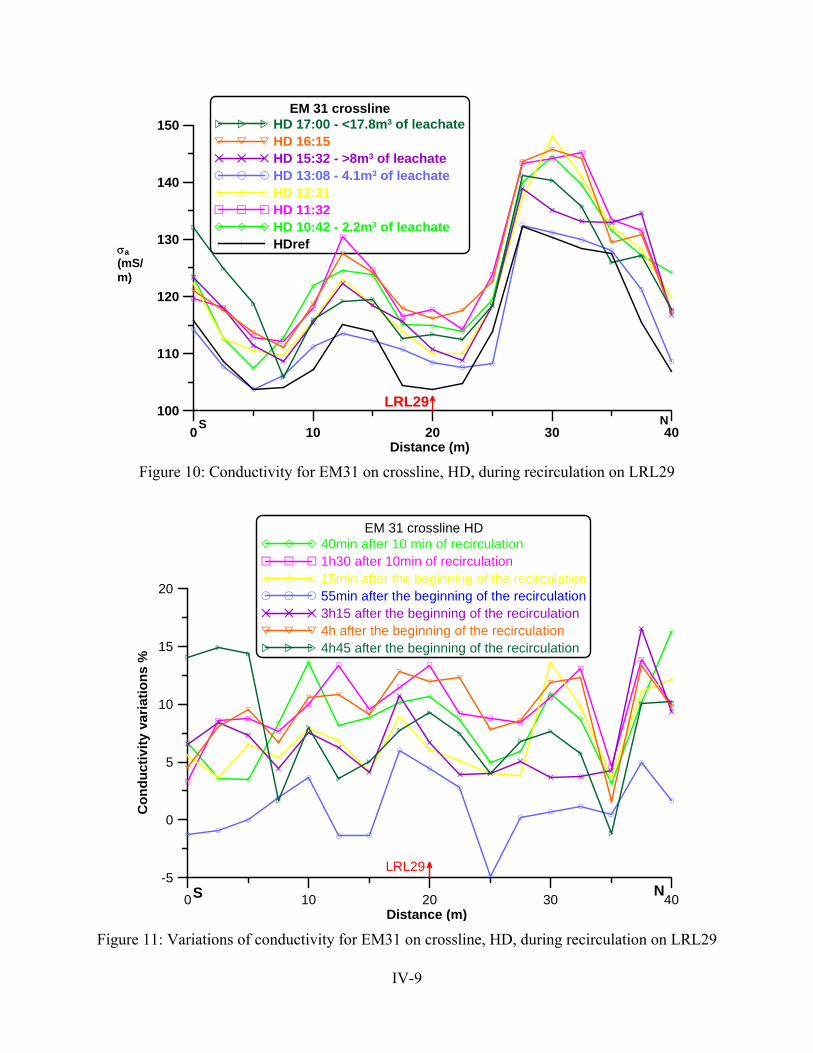
IV-9

0 10 20 30 40Distance (m)

100

110

120

130

140

150C

ondu

ctiv

ity (m

S/cm

)

EM 31 crosslineHD 17:00 - <17.8m3 of leachateHD 16:15HD 15:32 - >8m3 of leachateHD 13:08 - 4.1m3 of leachateHD 12:31HD 11:32HD 10:42 - 2.2m3 of leachateHDref

S NLRL29

Figure 10: Conductivity for EM31 on crossline, HD, during recirculation on LRL29

0 10 20 30 40Distance (m)

-5

0

5

10

15

20

Con

duct

ivity

var

iatio

ns %

EM 31 crossline HD40min after 10 min of recirculation1h30 after 10min of recirculation15min after the beginning of the recirculation55min after the beginning of the recirculation3h15 after the beginning of the recirculation4h after the beginning of the recirculation4h45 after the beginning of the recirculation

S NLRL29

Figure 11: Variations of conductivity for EM31 on crossline, HD, during recirculation on LRL29

σa (mS/m)

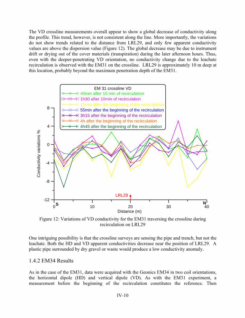
IV-10

The VD crossline measurements overall appear to show a global decrease of conductivity along the profile. This trend, however, is not consistent along the line. More importantly, the variations do not show trends related to the distance from LRL29, and only few apparent conductivity values are above the dispersion value (Figure 12). The global decrease may be due to instrument drift or drying out of the cover materials (transpiration) during the later afternoon hours. Thus, even with the deeper-penetrating VD orientation, no conductivity change due to the leachate recirculation is observed with the EM31 on the crossline. LRL29 is approximately 10 m deep at this location, probably beyond the maximum penetration depth of the EM31.

0 10 20 30 40Distance (m)

-12

-8

-4

0

4

8

Con

duct

ivity

var

iatio

ns %

EM 31 crossline VD40min after 10 min of recirculation1h30 after 10min of recirculation15min after the beginning of the recirculation55min after the beginning of the recirculation3h15 after the beginning of the recirculation4h after the beginning of the recirculation4h45 after the beginning of the recirculation

S N

LRL29

Figure 12: Variations of VD conductivity for the EM31 traversing the crossline during

recirculation on LRL29

One intriguing possibility is that the crossline surveys are sensing the pipe and trench, but not the leachate. Both the HD and VD apparent conductivities decrease near the position of LRL29. A plastic pipe surrounded by dry gravel or waste would produce a low conductivity anomaly. 1.4.2 EM34 Results As in the case of the EM31, data were acquired with the Geonics EM34 in two coil orientations, the horizontal dipole (HD) and vertical dipole (VD). As with the EM31 experiment, a measurement before the beginning of the recirculation constitutes the reference. Then

IV-11

measurements are made during the recirculation. The variations between the conductivity at the

time t, and the reference, is defined by t

ref

100 ln( )σ×

σ, expressed as a percentage. An positive

variation indicates a conductivity increase. Experiments conducted before leachate recirculation suggest that the dispersion for EM34 data collected within a short time interval are about 4% for the HD and 13% for the VD orientation. The somewhat larger dispersion for the VD orientation, in comparison to the EM31, may be due to coil misalignment since coils need to be laid down on the ground in a coplanar configuration. This is difficult to accomplish on a sloping landfill. The EM34 HD with a coil spacing of 10 m has a maximum penetration depth of 7.5 m, and is not supposed to see below the LRL (except at the edges of LRL29), contrary to the VD (maximum investigation depth of 15 m). With a coil spacing of 20 m, both dipoles should see deep enough to map the LRL and any leachate that accumulates adjacent to it. The negative recorded conductivities have been removed from the data and a 3-point moving average is applied to reduce the data noise. Negative conductivities are most likely caused by the presence of buried metal, producing a high induction number in the vicinity of the transmitter and receiver. Field observations suggest scatter in the data is primarily caused by coil misalignment along the sides of the landfill. This is particularly evident in the VD measurements, where coils were at different elevations, non-horizontal, and certainly not coplanar. Thus a 3-point moving average filter was used to reduce these variations, without over-smoothing the data. The 3-point moving average filter is essentially a “low-pass” filter that allows long-wavelength variations but removes short-wavelength variations. Alongstream Line Leachate recirculation along LRL29 appears to have little effect on the HD conductivity measurements (Figures 13 and 14) for data collected along the Alongstream Line. The variations are all in the range of the dispersion (Figure 13, in fact, shows pre- and post-injection values plotting on top of each other). The 20 m dipole spacing records higher apparent conductivity than the 10 m dipole, suggesting an overall increase in conductivity with depth. On the Alongstream Line, the VD orientation with the 10 and 20 m coil spacing (Figures 15, 16 and 17) clearly show a significant increase of conductivity at the beginning of the LRL (east end of perforated interval), in the middle, and at the end. For the 10 m coil spacing (with a maximum investigation depth of 15 m) the increase starts just at the beginning of the perforated interval and extends westward about 20 m.

IV-12

0 40 80 120 160 200Distance (m)

-40

0

40

80

120

160C

ondu

ctiv

ity (m

S/c

m)

EM 34 alongstreamHD ref_10mHD post_10mHD ref_20mHD post_20m

240

260

280

300

320E

levation (m)

E W

cell surface

LRL29

Figure 13: Conductivity measurements with EM34 on the Alongstream Line, HD orientation,

during recirculation on LRL29, smoothed with a 3-point moving average

0 40 80 120 160 200Distance (m)

-20

-10

0

10

20

Con

duct

ivity

var

iatio

ns %

EM 34 alongstreamHD post-ref_10mHD post-ref_20m

240

260

280

300

320

Elevation (m

)

E W

cell surfaceLRL29

Figure 14: Variations of conductivity collected with the EM34 on the Alongstream Line, HD,

during recirculation on LRL29 (June), with a 3-point moving average filter, with the dispersion range between the outer dashed lines (4%)

coil spacing (with a maximum investigation depth of 30 m) the increase also starts near the east end of the perforated interval. A second zone of increased apparent conductivity occurs near the west end of the perforated interval (Figure 16). Post-injection apparent conductivity is actually lower along the middle of the perforated interval in the 10 or 20 m coil spacing measurements.

σa (mS/m)

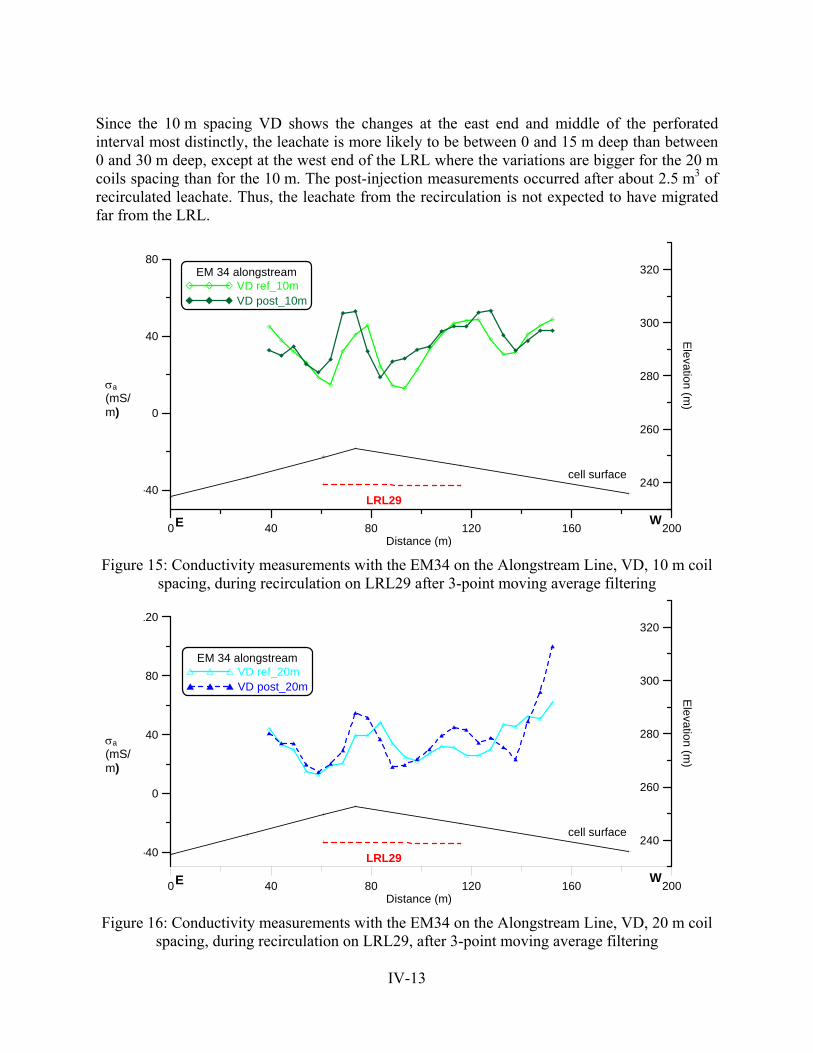
IV-13

Since the 10 m spacing VD shows the changes at the east end and middle of the perforated interval most distinctly, the leachate is more likely to be between 0 and 15 m deep than between 0 and 30 m deep, except at the west end of the LRL where the variations are bigger for the 20 m coils spacing than for the 10 m. The post-injection measurements occurred after about 2.5 m3 of recirculated leachate. Thus, the leachate from the recirculation is not expected to have migrated far from the LRL.

0 40 80 120 160 200Distance (m)

-40

0

40

80

Con

duct

ivity

(mS

/cm

)

EM 34 alongstreamVD ref_10mVD post_10m

240

260

280

300

320

Elevation

(m)

E W

cell surface

LRL29

Figure 15: Conductivity measurements with the EM34 on the Alongstream Line, VD, 10 m coil

spacing, during recirculation on LRL29 after 3-point moving average filtering

0 40 80 120 160 200Distance (m)

-40

0

40

80

120

Con

duct

ivity

(mS

/cm

)

EM 34 alongstreamVD ref_20mVD post_20m

240

260

280

300

320

Elevation

(m)

E W

cell surface

LRL29

Figure 16: Conductivity measurements with the EM34 on the Alongstream Line, VD, 20 m coil

spacing, during recirculation on LRL29, after 3-point moving average filtering

σa (mS/m)

σa (mS/m)

IV-14

0 40 80 120 160 200Distance (m)

EM 34 alongstreamVD post-ref_10mVD post-ref_20m

240

260

280

300

320E

levation (m)

-100

-50

0

50

100C

ondu

ctiv

ity v

aria

tions

%

E W

cell surfaceLRL29

Figure 17: Variations of conductivity with the EM34 on the Alongstream Line, VD, during recirculation on LRL29 (June). A 3-point moving average was applied to the data, with the

dispersion range (13%) indicated by the outer dashed lines

HD conductivity measurements with a coil spacing of 20 m have approximately the same investigation depth as the VD orientation with the coil spacing of 10 m. Nevertheless the observed variations and the range are very different (Figure 18), perhaps reflecting a high degree of anisotropy in the subsurface, since coils in the HD and VD orientations excite currents in the ground differently. The VD 10 and 20 m response near the center of LRL29 also appears inconsistent. Figure 17 shows this dramatic discordance. The VD 10 m shows a conductivity increase of almost 75% whereas the VD 20 m spacing records a conductivity decrease of similar magnitude. The response of the VD 10 and 20 m spacing near the ends of LRL29 are more consistent in indicating increased conductivity, especially on the east (injection) end. Upstream Line Measurements on the Upstream Line have been carried out during the recirculation along LRL28 (May, 17-18) and on LRL29 (June, 1-2). The 10 m EM post-injection measurements occurred after 0.3 and 4 m3 of leachate were injected on May 18 and June 2, respectively, and the 20 m coil spacing experiments after 0.3 and 5.5 m3 were injected on May 18 and June 2, respectively.

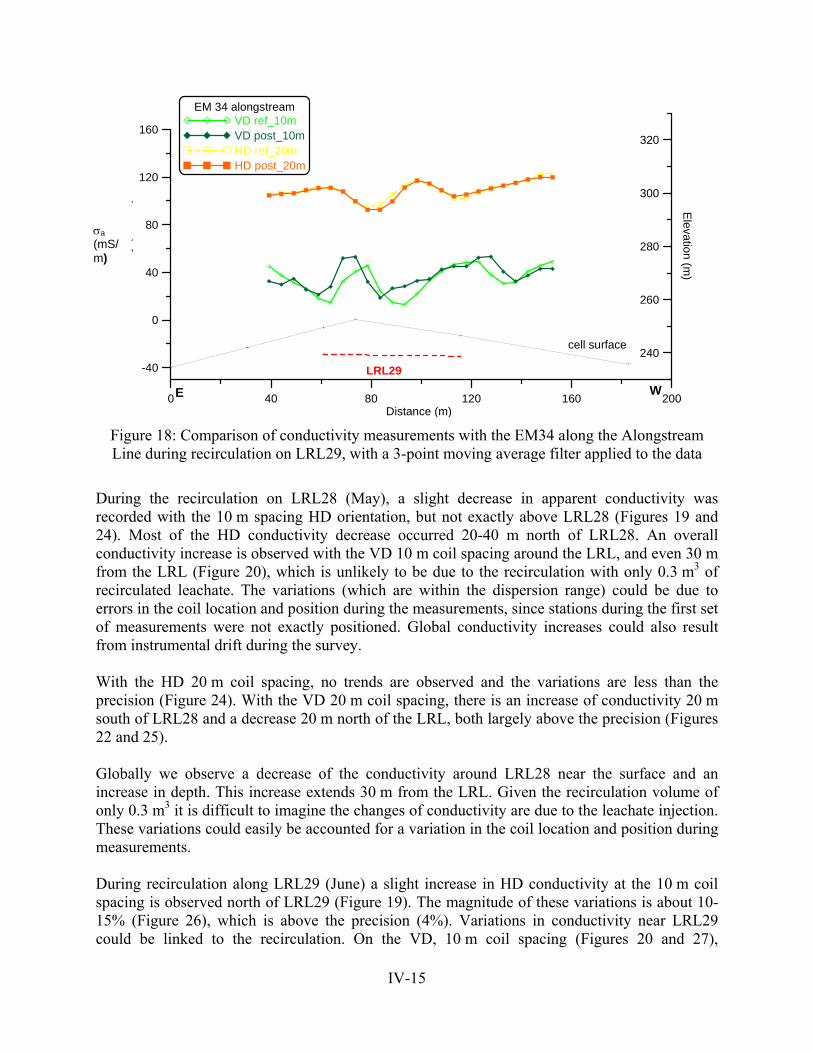
IV-15

0 40 80 120 160 200Distance (m)

-40

0

40

80

120

160C

ondu

ctiv

ity (m

S/c

m)

EM 34 alongstreamVD ref_10mVD post_10mHD ref_20mHD post_20m

240

260

280

300

320Elevation (m

)

E W

cell surface

LRL29

Figure 18: Comparison of conductivity measurements with the EM34 along the Alongstream Line during recirculation on LRL29, with a 3-point moving average filter applied to the data

During the recirculation on LRL28 (May), a slight decrease in apparent conductivity was recorded with the 10 m spacing HD orientation, but not exactly above LRL28 (Figures 19 and 24). Most of the HD conductivity decrease occurred 20-40 m north of LRL28. An overall conductivity increase is observed with the VD 10 m coil spacing around the LRL, and even 30 m from the LRL (Figure 20), which is unlikely to be due to the recirculation with only 0.3 m3 of recirculated leachate. The variations (which are within the dispersion range) could be due to errors in the coil location and position during the measurements, since stations during the first set of measurements were not exactly positioned. Global conductivity increases could also result from instrumental drift during the survey. With the HD 20 m coil spacing, no trends are observed and the variations are less than the precision (Figure 24). With the VD 20 m coil spacing, there is an increase of conductivity 20 m south of LRL28 and a decrease 20 m north of the LRL, both largely above the precision (Figures 22 and 25). Globally we observe a decrease of the conductivity around LRL28 near the surface and an increase in depth. This increase extends 30 m from the LRL. Given the recirculation volume of only 0.3 m3 it is difficult to imagine the changes of conductivity are due to the leachate injection. These variations could easily be accounted for a variation in the coil location and position during measurements. During recirculation along LRL29 (June) a slight increase in HD conductivity at the 10 m coil spacing is observed north of LRL29 (Figure 19). The magnitude of these variations is about 10-15% (Figure 26), which is above the precision (4%). Variations in conductivity near LRL29 could be linked to the recirculation. On the VD, 10 m coil spacing (Figures 20 and 27),

σa (mS/m)

IV-16

conductivity variations are quite high, and occur also above LRL28 and 29. There is a decrease of conductivity above LRL28, an increase north of LRL28 and an increase in conductivity north of LRL29. With the 10 m coil spacing, the slight conductivity increase north of LRL29 could be due to leachate recirculation. If so, this indicates leachate extending almost 20 m north of the LRL in the shallow waste. The HD, 20 m coil spacing, shows an increase of the conductivity on the side of LRL28 and a decrease around LRL29 (Figures 26 and 27). The VD 20 m coil spacing apparent conductivities shows an increase of the conductivity south of LRL28 and a decrease north of LRL29, both largely above the precision. With the 20 m coil spacing, the trend is exactly opposite to that expected if leachate recirculation was being observed: the conductivity decreases around LRL29. These complex results suggest neither the HD nor the VD could be used to map leachate infiltration along the Upstream Line. Too many other factors affect apparent conductivity along this line. Apparent conductivity values also vary between the HD with 20 m coil spacing and the VD with 10 m coil spacing. This is somewhat surprising since both supposed to have an investigation depth of approximately 15 m (Figure 23). If the trend at the beginning of the line is a bit similar (increasing apparent conductivity south of LRL28), the conductivity values are very different between the two dipoles. The influence of the coil location and inclination on the measurements should be investigated in order to try to explain these observed variations.

0 20 40 60 80 100 120Distance (m)

0

50

100

150

200

250

Con

duct

ivity

(mS

/cm

)

EM 34 upstream_HD_10m5/17/06_pre5/18/06_post6/1/06_pre6/2/06_post

240

260

280

300

320

Elevation

(m)

S N

cell surface

LRL29LRL28

Figure 19: Conductivity with EM34 on Upstream, HD, 10 m coil spacing, during recirculation on

LRL28 (May) and LRL29 (June), with a 3-point moving average applied

σa (mS/m)

IV-17

0 40 80 120Distance (m)

-100

0

100

200

Con

duct

ivity

(mS

/cm

)EM 34 upstream_VD_10m

5/17/06_pre5/18/06_post6/1/06_pre6/2/06_post

240

260

280

300

320E

levation (m)

S N

cell surface

LRL29LRL28

Figure 20: Conductivity with the EM34 on the Upstream Line, VD, 10 m coil spacing, during recirculation on LRL28 (May) and LRL29 (June), after a 3-point moving average was applied

0 40 80 120Distance (m)

80

120

160

200

240

Con

duct

ivity

(mS

/cm

)

EM 34 upstream_HD_20m5/18/06_pre5/18/06_post6/1/06_pre6/1/06_post

240

260

280

300

320

Elevation (m

)

S N

cell surface

LRL29LRL28

Figure 21: Conductivity with EM34 on the Upstream Line, HD, 20 m coil spacing, during

recirculation on LRL28 (May) and 29 (June), after 3-point moving averaging

σa (mS/m)

σa (mS/m)

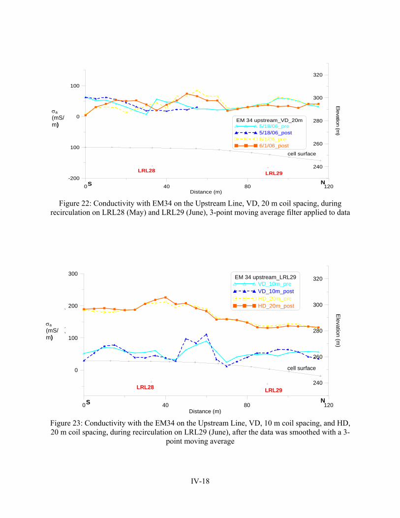
IV-18

0 40 80 120Distance (m)

-200

-100

0

100

Con

duct

ivity

(mS

/cm

)

EM 34 upstream_VD_20m5/18/06_pre5/18/06_post6/1/06_pre6/1/06_post

240

260

280

300

320

Elevation (m

)

S N

cell surface

LRL29LRL28

Figure 22: Conductivity with EM34 on the Upstream Line, VD, 20 m coil spacing, during

recirculation on LRL28 (May) and LRL29 (June), 3-point moving average filter applied to data

0 40 80 120Distance (m)

0

100

200

300

Con

duct

ivity

(mS

/cm

)

EM 34 upstream_LRL29VD_10m_preVD_10m_postHD_20m_preHD_20m_post

240

260

280

300

320

Elevation

(m)

S N

cell surface

LRL29LRL28

Figure 23: Conductivity with the EM34 on the Upstream Line, VD, 10 m coil spacing, and HD, 20 m coil spacing, during recirculation on LRL29 (June), after the data was smoothed with a 3-

point moving average

σa (mS/m)

σa (mS/m)

IV-19

0 40 80 120Distance (m)

-20

-15

-10

-5

0

5C

ondu

ctiv

ity v

aria

tions

%

EM 34 upstreamHD post-ref_10mHD post-ref_20m

240

260

280

300

320E

levation (m)

S N

cell surface

LRL29LRL28

Figure 24: Variations of conductivity with the EM34 on the Upstream Line, HD, during

recirculation on LRL28 (May), 3-point moving average applied, with dispersion range (4%), shown by outer dashed lines

0 40 80 120Distance (m)

-150

-100

-50

0

50

100

150

Con

duct

ivity

var

iatio

ns %

EM 34 upstreamVD post-ref_10mVD post-ref_20m

240

260

280

300

320

Elevation (m

)

S N

cell surface

LRL29LRL28

Figure 25: Variations of conductivity with EM34 on the Upstream Line, VD, during recirculation

on LRL28 (May), 3-point moving average applied, dispersion range 13%

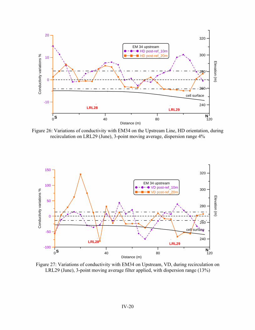
IV-20

0 40 80 120Distance (m)

-10

0

10

20C

ondu

ctiv

ity v

aria

tions

%

EM 34 upstreamHD post-ref_10mHD post-ref_20m

240

260

280

300

320E

levation (m)

S N

cell surface

LRL29LRL28

Figure 26: Variations of conductivity with EM34 on the Upstream Line, HD orientation, during

recirculation on LRL29 (June), 3-point moving average, dispersion range 4%

0 40 80 120Distance (m)

-100

-50

0

50

100

150

Con

duct

ivity

var

iatio

ns %

EM 34 upstreamVD post-ref_10mVD post-ref_20m

240

260

280

300

320

Elevation

(m)

S N

cell surface

LRL29LRL28

Figure 27: Variations of conductivity with EM34 on Upstream, VD, during recirculation on

LRL29 (June), 3-point moving average filter applied, with dispersion range (13%)

IV-21

1.5 Long-term Conductivity Changes 1.5.1 EM31 Surveys On July 31, 2007, EM conductivity surveys were repeated along the Upstream and Alongstream Lines. Both the EM31 and EM34 were used to measure apparent conductivity. EM conductivity was then compared with data collected during 2006, to assess long-term conductivity changes that may relate to degradation of the refuse, diffusion of leachate through the refuse, or changes in cover conditions. Please note that the coordinate system for plotting these profiles (Figures 28-34) differs from the previous profile plots: here the east end of the profile is at the start of the ERT lines, not the base of the landfill slope. Smoothing was not applied to this data and variance was also not analyzed in a quantitative manner. Upstream Line Results of EM31 surveys along the Upstream Line are shown in Figure 28. Locations of LRL28 and 29 are also shown by the open ovals. The overall decreasing conductivity trend, from south to north, occurs in both the May, 2006 and July, 2007 data. Apparent conductivity values recorded in 2007 are considerably lower, however, than values recorded in 2006. VD conductivities decrease from 10-30 mS/m, and HD conductivities decrease 10-90 mS/m along the line. The only anomalous behavior associated with the LRLs is that the HD conductivity for 2007 shows a 40 mS/m decrease centered on LRL28. As the HD for the EM31 is only sensitive to the upper 2.8 m or so, this probably reflects some sort of surficial effect. The 2007 data, on the whole, however, appear much smoother than the 2006 data.

Upstream line -- EM31

0

50

100

150

200

250

0 20 40 60 80 100 120 140

D ist ance ( m)

VD (5/18/06)HD (5/18/06)VD (7/31/07)HD (7/31/07)

S NLR L2 8 LR L2 9

Figure 28: Long-term changes in apparent conductivity on the Upstream Line, as recorded with the EM31. Positions of LRL28 and LRL29 are also shown

σa (mS/m)

IV-22

Alongstream Line Long-term changes in apparent conductivity were also examined with the EM31 on the Alongstream Line. Figure 29 shows the results. Again, the 2007 apparent conductivity values were significantly lower than the 2006 values. The perforated interval of LRL29 is also shown on Figure 29. The perforated interval appears to have no influence on apparent conductivity values, suggesting the EM31 is sensing only very shallow conductivity.

Alongstream EM31

0

50

100

150

200

250

0 20 40 60 80 100 120 140

Distance (m)

App

aren

t con

duct

ivity

(mS/

m)

VD (6/1/06)HD (6/1/06)VD (7/31/07)HD (7/31/07)

E WPerforations

Figure 29: Long-term changes in apparent conductivity as measured with the EM31 on the Alongstream Line High-resolution Crossline Figure 30 shows the Crossline conductivity in 2007, as compared with the 2006 values along the same line. Values obtained in 2007 are much lower than those measured in 2006 (by 20-80 mS/ms) and the 2007 values are smoother (exhibit less variance). There is no apparent influence of LRL29 on the EM31 data.

IV-23

EM31 Crossline

0

20

40

60

80

100

120

140

0 5 10 15 20 25 30 35 40 45

Distance (m)

App

aren

t con

duct

ivity

(mS/

m)

VD (6/1/06)

HD (6/1/06)

VD (7/31/07)

HD (7/31/07)

S NLRL29

Figure 30: Long-term apparent conductivity changes on the Crossline over LRL29, as measured with the EM31 1.5.2 EM34 Surveys Upstream Line Figure 31 shows the 2007 Upstream Line apparent conductivity values, as recorded with an EM34, with a 10 m coil separation. Figure 32 shows 2007 apparent conductivities, as recorded with an EM34 at a 20 m separation. VD conductivity at the 10 m spacing, recorded during 2007, is, on average, is slightly higher or about the same as the apparent conductivity recorded during 2006. However, the 2007 data shows much less variability than the 2006 data. The HD data show both increases and decreases in apparent conductivity between 2006 and 2007. Figure 31. Long term apparent conductivity changes on the Upstream Line, as recorded with the EM34 at a 10 m dipole spacing. Figure 32 shows the Upstream Line profile as recorded with the EM34 at a 20 m spacing. The HD data tracks on top of each other, indicating no change in HD conductivity. The VD conductivity shows an increase in apparent conductivity in the 2007 data, suggesting the deeper refuse is more conductive. The 2007 data is also less variable.

IV-24

Upstream Line EM34 10 m

-100

-50

0

50

100

150

200

250

0 20 40 60 80 100 120 140

D ist ance ( m)

VD (5/17/06)HD (5/17/06)VD (7/31/07)HD (7/31/07)

S NLR L2 8 LR L2 9

Figure 31: Long-term apparent conductivity changes on the Upstream Line, as recorded with the EM34 at a 10 m dipole spacing

Upstream Line EM34 20 m

-100

-50

0

50

100

150

200

250

300

0 20 40 60 80 100 120 140

Distance (m)

App

aran

t con

duct

ivity

(mS/

m)

VD (5/18/06)

HD (5/18/06)

VD (7/31/07)

HD (7/31/07)

LRL28 LRL29S N

Figure 32. Long-term apparent conductivity changes on the Upstream Line, as recorded with the EM34 at a 20 m dipole spacing

σa (mS/m)

IV-25

Alongstream Line Figures 33 and 34 show changes in the Alongstream Line apparent conductivity data as recorded with the EM34 at dipole spacings of 10 m and 20 m, respectively. Higher apparent conductivities are recorded in 2007 in the VD orientation. In the case of the 20 m dipole data, the VD apparent conductivities are 20-90 mS/m higher than those measured in 2006. The horizontal dipole (HD) for 2007 is about 0-25 mS/m higher than those collected in 2006, in some cases. In other cases the HD conductivities are unchanged, or actually lower in 2007. The greater increase in VD conductivity suggests the deeper refuse is more conductive, perhaps as a result of the repeated leachate injections.

Alongstream Line EM34 10 m

-20

0

20

40

60

80

100

120

140

0 20 40 60 80 100 120 140

Distance (m)

App

aran

t con

duct

ivity

(mS/

m)

VD (6/1/06)

HD (6/1/06)

VD (7/31/07)

HD (7/31/07)

Perforations

E W

Figure 33: Long-term apparent conductivity changes on the Alongstream Line, as recorded with the EM34 at a 10 m dipole spacing

IV-26

Alongstream Line - EM34 20 m

-20

0

20

40

60

80

100

120

140

160

0 20 40 60 80 100 120 140

D ist ance ( m)

VD (6/1/06)HD (6/1/06)VD (7/31/07)HD (7/31/07)

E WPerf orat io ns

Figure 34: Long-term apparent conductivity changes on the Alongstream Line, as recorded with the EM34 at 20 m dipole spacing 1.6 EM Method Conclusions Data suggests the EM31 was unable to detect leachate due to its shallow response depth. The EM34 appears to have detected leachate along LRL29 when the EM profile was along and directly over LRL29. Significant increases in apparent conductivity were measured by the EM34 near the east and west ends of the perforated portion of LRL29. This pattern of conductivity increases suggest leachate injection was not homogeneous along the line. EM conductivity profiles perpendicular to the LRLs were of little use in identifying leachate (i.e. the Alongstream and Crosslines). In one case a zone of increased conductivity 10 to 20 m north of LRL29 may indicate possible leachate migration north of the perforated interval. Surveys made during the summer of 2007, approximately one year after final cover emplacement, suggest near-surface conductivity has decreased substantially, whereas conductivity of the deeper refuse has increased. Shallow cover materials may have dried out, leading to lower conductivity, whereas the higher conductivity of the lower refuse over time may indicate infiltration by recirculating leachate or waste biodegradation. Specifically, (1) At the Orchard Hills Landfill conductivity measurements must be made with EM coils separated by at least 10 m to have sufficient depth sensitivity to detect leachate. Shallower instruments, however, (such as the Geonics EM31), although not able to detect leachate, may provide useful data on temporal conductivity variations. For example, daily conductivity variations of as much as 20 mS/m were recorded over portions of the bioreactor cell.

σa (mS/m)

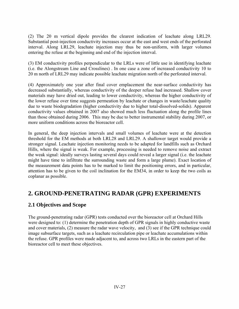
IV-27

(2) The 20 m vertical dipole provides the clearest indication of leachate along LRL29. Substantial post-injection conductivity increases occur at the east and west ends of the perforated interval. Along LRL29, leachate injection may thus be non-uniform, with larger volumes entering the refuse at the beginning and end of the injection interval. (3) EM conductivity profiles perpendicular to the LRLs were of little use in identifying leachate (i.e. the Alongstream Line and Crosslines) . In one case a zone of increased conductivity 10 to 20 m north of LRL29 may indicate possible leachate migration north of the perforated interval. (4) Approximately one year after final cover emplacement the near-surface conductivity has decreased substantially, whereas conductivity of the deeper refuse had increased. Shallow cover materials may have dried out, leading to lower conductivity, whereas the higher conductivity of the lower refuse over time suggests permeation by leachate or changes in waste/leachate quality due to waste biodegradation (higher conductivity due to higher total-dissolved-solids). Apparent conductivity values obtained in 2007 also showed much less fluctuation along the profile lines than those obtained during 2006. This may be due to better instrumental stability during 2007, or more uniform conditions across the bioreactor cell. In general, the deep injection intervals and small volumes of leachate were at the detection threshold for the EM methods at both LRL28 and LRL29. A shallower target would provide a stronger signal. Leachate injection monitoring needs to be adapted for landfills such as Orchard Hills, where the signal is weak. For example, processing is needed to remove noise and extract the weak signal: ideally surveys lasting several days could reveal a larger signal (i.e. the leachate might have time to infiltrate the surrounding waste and form a large plume). Exact location of the measurement data points has to be marked to limit the positioning errors, and in particular, attention has to be given to the coil inclination for the EM34, in order to keep the two coils as coplanar as possible. 2. GROUND-PENETRATING RADAR (GPR) EXPERIMENTS

2.1 Objectives and Scope The ground-penetrating radar (GPR) tests conducted over the bioreactor cell at Orchard Hills were designed to: (1) determine the penetration depth of GPR signals in highly conductive waste and cover materials, (2) measure the radar wave velocity, and (3) see if the GPR technique could image subsurface targets, such as a leachate recirculation pipe or leachate accumulations within the refuse. GPR profiles were made adjacent to, and across two LRLs in the eastern part of the bioreactor cell to meet these objectives.

IV-28

2.2 Ground- Penetrating Radar: How Does It Work?

2.2.1 General Theory GPR is a noninvasive technique for high-resolution geophysical mapping of the shallow subsurface. It is often used to identify the water table, layers and sedimentary structures in soil, the bedrock surface, fractures, faults, buried waste pits, buried pipes, tanks, and voids in the subsurface. GPR output is a picture-like display, consisting of radar waveforms plotted as time vs. position (side-by-side) “traces.” The display looks like a geological cross-section, but important differences exist. Some signals on the sections may arise from above-ground reflections. Other distortions may also occur such as diffractions from point reflectors, ringing from multiple reflections, etc. For this reason apparent reflections are called “events” on the radar sections. Reflection times on GPR sections are usually specified in nanoseconds (ns) – a nanosecond is 1 x 10-9 s. Radar waves originate at a transmitting antenna at the ground surface, bounce off layers or structures with contrasting dielectric permittivity, and are received at the surface by another receiving antenna. Dielectric permittivity is highly dependent on the water content, and in coarse-grained materials, the water table is often associated with a strong radar reflection that cuts across other events. Most data collection is very simple: two antennas are simply marched down the profile line at a fixed spacing (Figures 35 and 36). Data is collected as antennas are stopped at each station for a few seconds to record reflections from radar pulses emitted by the transmitter. Stations are usually separated by a few 10s of cm, to provide dense lateral resolution. The results are plotted as a time or depth section showing the returned (reflected) radar waveforms at the transmitter (Tx) – receiver (Rx) midpoint. These may be colored or shaded to enhance certain features. Usually an initial walkway, or common-midpoint (CMP) survey, is performed to obtain the radar wave velocity. The topmost (earliest) reflections are always the air-wave and ground-wave, which should be ignored in the interpretation.

Figure 35: Bistatic (two-antenna) GPR system showing air, ground and reflected waves. Tx represents the transmitter and Rx the receiver (after Annan and Cosway, 1992)

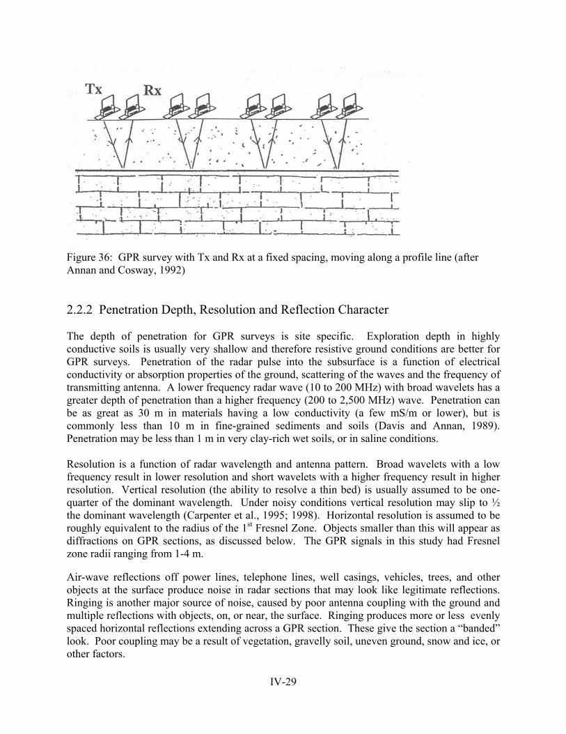
IV-29

Figure 36: GPR survey with Tx and Rx at a fixed spacing, moving along a profile line (after Annan and Cosway, 1992) 2.2.2 Penetration Depth, Resolution and Reflection Character The depth of penetration for GPR surveys is site specific. Exploration depth in highly conductive soils is usually very shallow and therefore resistive ground conditions are better for GPR surveys. Penetration of the radar pulse into the subsurface is a function of electrical conductivity or absorption properties of the ground, scattering of the waves and the frequency of transmitting antenna. A lower frequency radar wave (10 to 200 MHz) with broad wavelets has a greater depth of penetration than a higher frequency (200 to 2,500 MHz) wave. Penetration can be as great as 30 m in materials having a low conductivity (a few mS/m or lower), but is commonly less than 10 m in fine-grained sediments and soils (Davis and Annan, 1989). Penetration may be less than 1 m in very clay-rich wet soils, or in saline conditions. Resolution is a function of radar wavelength and antenna pattern. Broad wavelets with a low frequency result in lower resolution and short wavelets with a higher frequency result in higher resolution. Vertical resolution (the ability to resolve a thin bed) is usually assumed to be one-quarter of the dominant wavelength. Under noisy conditions vertical resolution may slip to ½ the dominant wavelength (Carpenter et al., 1995; 1998). Horizontal resolution is assumed to be roughly equivalent to the radius of the 1st Fresnel Zone. Objects smaller than this will appear as diffractions on GPR sections, as discussed below. The GPR signals in this study had Fresnel zone radii ranging from 1-4 m. Air-wave reflections off power lines, telephone lines, well casings, vehicles, trees, and other objects at the surface produce noise in radar sections that may look like legitimate reflections. Ringing is another major source of noise, caused by poor antenna coupling with the ground and multiple reflections with objects, on, or near, the surface. Ringing produces more or less evenly spaced horizontal reflections extending across a GPR section. These give the section a “banded” look. Poor coupling may be a result of vegetation, gravelly soil, uneven ground, snow and ice, or other factors.

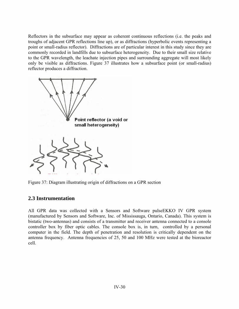
IV-30

Reflectors in the subsurface may appear as coherent continuous reflections (i.e. the peaks and troughs of adjacent GPR reflections line up), or as diffractions (hyperbolic events representing a point or small-radius reflector). Diffractions are of particular interest in this study since they are commonly recorded in landfills due to subsurface heterogeneity. Due to their small size relative to the GPR wavelength, the leachate injection pipes and surrounding aggregate will most likely only be visible as diffractions. Figure 37 illustrates how a subsurface point (or small-radius) reflector produces a diffraction.

Figure 37: Diagram illustrating origin of diffractions on a GPR section

2.3 Instrumentation All GPR data was collected with a Sensors and Software pulseEKKO IV GPR system (manufactured by Sensors and Software, Inc. of Mississauga, Ontario, Canada). This system is bistatic (two-antennas) and consists of a transmitter and receiver antenna connected to a console controller box by fiber optic cables. The console box is, in turn, controlled by a personal computer in the field. The depth of penetration and resolution is critically dependent on the antenna frequency. Antenna frequencies of 25, 50 and 100 MHz were tested at the bioreactor cell.

IV-31

2.4 GPR Surveys Over the Orchard Hills Bioreactor Cell

2.4.1 Location of Surveys Seventeen GPR surveys were made during two days of fieldwork on July 20 and August 1, 2007. These surveys fall into the following four groups: (a) common-midpoint surveys to assess velocity, (b) south-to-north traverses across LRL29, located 10 m west of LRW29 (referred to here as along Profile A), (c) south-to-north traverses across LRL29, located 30 m west of LRW29 (Profile B), and (d) a single south-to-north profile across LRL28, located 22 m west of LRW28 (Profile C). It was hoped that the GPR profiles across LRL28 and LRL29 would image the leachate recirculation line or leachate migrating into the refuse. Figure 38 shows the line locations near LRW29.

Figure 38: GPR surveys over LRL29

2.4.2 Timing of Surveys and Leachate Injection Only 50 and 100 MHz antennas were used along Profile A during the 2007 surveys. Profile lines B and C were collected on August 1, 2007. During the August 1 surveys leachate clearly was being injected (we could hear the leachate moving through LRW29). On July 20 we heard no leachate being injected, although some may have been injected earlier in the day, before we started our surveys. GPR surveys using 25 and 50 MHz antennas were repeated along Profile B before and during leachate injection on July 29, 2008. 2.4.3 Determining GPR wave Velocity Using CMP Surveys As noted above, in most GPR investigations the first surveys are designed to measure radar wave velocity in the earth. This velocity will be slightly less than the speed of light, and the velocity of the radar wave depends on the subsurface materials. Moist clayey materials have lower velocity than dry sandy or gravelly materials. So at the bioreactor cell the first surveys were CMP surveys in which the GPR wave velocity was measured by slowly separating the transmitting and receiving antennas about a common midpoint. The location of the CMP

IV-32

surveys was about 10-20 m south of LRL29, to avoid encountering anomalous soil conditions associated with the LRL. In our case the GPR signal was recorded at 0.2 m separation intervals to a total separation of about 5 m. From these records the air- and ground-waves show different slopes, corresponding to their velocities. Figure 39 shows a CMP record that gave an air-wave velocity of 0.30 m/ns (meters/nanosecond) and a ground-wave velocity of about 0.086 m/ns. The air-wave velocity is constant at all locations and is a good way to check the timing system. The ground-wave velocity is reasonable for clayey cap materials, although the refuse probably exhibits a lower velocity. This velocity was used to convert reflection times to depth on the GPR sections.

Figure 39: GPR common-midpoint velocity survey at Orchard Hills 2.4.4 GPR Profiles Across the Leachate Recirculation Lines (LRLs) South-to-north profiles across LRL29 are labeled Profiles A and B; the sole profile across LRL28 is labeled Profile C. Profile A was 20 m long, oriented north-south, and located 10 m west of LRW29, at the approximate east end of the alongstream electrical resistivity tomography (ERT) line collected by Solenne Grellier. Profiles A and B cross LRL29 near their centers (about the 10 m station). Profile B was made along a north-south line 30 m west of LRW29, and the C profile was made 22 m west of LRW28. Profile C also crosses LRL28 at about position 10 m. Profiles are presented in order of decreasing frequency, which corresponds to increasing depth. Cross-sections compiled from engineering drawings of the bioreactor cell beneath each profile are shown in Figures 40 and 41.

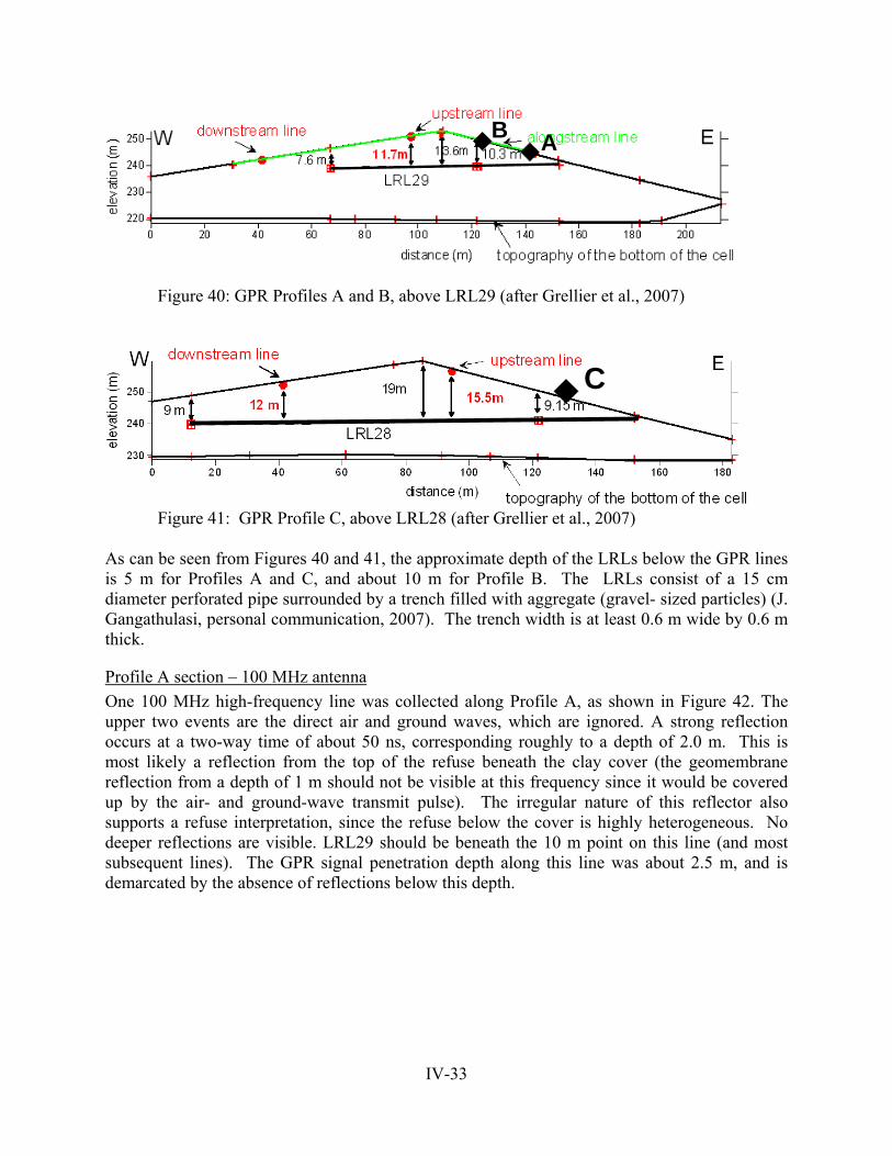
IV-33

AB

Figure 40: GPR Profiles A and B, above LRL29 (after Grellier et al., 2007)

C

Figure 41: GPR Profile C, above LRL28 (after Grellier et al., 2007) As can be seen from Figures 40 and 41, the approximate depth of the LRLs below the GPR lines is 5 m for Profiles A and C, and about 10 m for Profile B. The LRLs consist of a 15 cm diameter perforated pipe surrounded by a trench filled with aggregate (gravel- sized particles) (J. Gangathulasi, personal communication, 2007). The trench width is at least 0.6 m wide by 0.6 m thick.

Profile A section – 100 MHz antenna One 100 MHz high-frequency line was collected along Profile A, as shown in Figure 42. The upper two events are the direct air and ground waves, which are ignored. A strong reflection occurs at a two-way time of about 50 ns, corresponding roughly to a depth of 2.0 m. This is most likely a reflection from the top of the refuse beneath the clay cover (the geomembrane reflection from a depth of 1 m should not be visible at this frequency since it would be covered up by the air- and ground-wave transmit pulse). The irregular nature of this reflector also supports a refuse interpretation, since the refuse below the cover is highly heterogeneous. No deeper reflections are visible. LRL29 should be beneath the 10 m point on this line (and most subsequent lines). The GPR signal penetration depth along this line was about 2.5 m, and is demarcated by the absence of reflections below this depth.

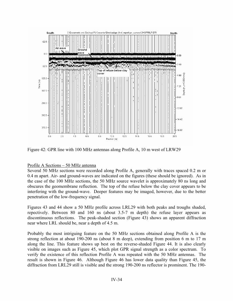
IV-34

Figure 42: GPR line with 100 MHz antennas along Profile A, 10 m west of LRW29 Profile A Sections – 50 MHz antenna Several 50 MHz sections were recorded along Profile A, generally with traces spaced 0.2 m or 0.4 m apart. Air- and ground-waves are indicated on the figures (these should be ignored). As in the case of the 100 MHz sections, the 50 MHz source wavelet is approximately 80 ns long and obscures the geomembrane reflection. The top of the refuse below the clay cover appears to be interfering with the ground-wave. Deeper features may be imaged, however, due to the better penetration of the low-frequency signal. Figures 43 and 44 show a 50 MHz profile across LRL29 with both peaks and troughs shaded, repectively. Between 80 and 160 ns (about 3.5-7 m depth) the refuse layer appears as discontinuous reflections. The peak-shaded section (Figure 43) shows an apparent diffraction near where LRL should be, near a depth of 4.5 m. Probably the most intriguing feature on the 50 MHz sections obtained along Profile A is the strong reflection at about 190-200 ns (about 8 m deep), extending from position 6 m to 17 m along the line. This feature shows up best on the reverse-shaded Figure 44. It is also clearly visible on images such as Figure 45, which plot GPR signal strength as a color spectrum. To verify the existence of this reflection Profile A was repeated with the 50 MHz antennas. The result is shown in Figure 46. Although Figure 46 has lower data quality than Figure 45, the diffraction from LRL29 still is visible and the strong 190-200 ns reflector is prominent. The 190-

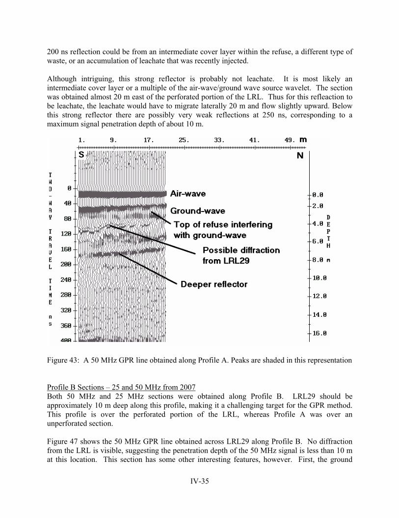
IV-35

200 ns reflection could be from an intermediate cover layer within the refuse, a different type of waste, or an accumulation of leachate that was recently injected. Although intriguing, this strong reflector is probably not leachate. It is most likely an intermediate cover layer or a multiple of the air-wave/ground wave source wavelet. The section was obtained almost 20 m east of the perforated portion of the LRL. Thus for this refleaction to be leachate, the leachate would have to migrate laterally 20 m and flow slightly upward. Below this strong reflector there are possibly very weak reflections at 250 ns, corresponding to a maximum signal penetration depth of about 10 m.

Figure 43: A 50 MHz GPR line obtained along Profile A. Peaks are shaded in this representation Profile B Sections – 25 and 50 MHz from 2007 Both 50 MHz and 25 MHz sections were obtained along Profile B. LRL29 should be approximately 10 m deep along this profile, making it a challenging target for the GPR method. This profile is over the perforated portion of the LRL, whereas Profile A was over an unperforated section. Figure 47 shows the 50 MHz GPR line obtained across LRL29 along Profile B. No diffraction from the LRL is visible, suggesting the penetration depth of the 50 MHz signal is less than 10 m at this location. This section has some other interesting features, however. First, the ground

IV-36

wave is slowed directly above the LRL. This may mean soil is less compacted over the LRL, or more moist. Also, between about 9.5 and 12 m along the line reflections seem to vanish, perhaps as a result of strong absorption of the GPR signal, or from backfilling the trench after emplacement of the LRL.

Figure 44: The same 50 MHz GPR line as shown in Figure 9, with troughs shaded

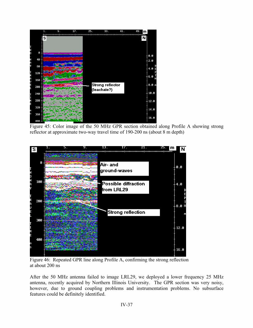
IV-37

Figure 45: Color image of the 50 MHz GPR section obtained along Profile A showing strong reflector at approximate two-way travel time of 190-200 ns (about 8 m depth)

Figure 46: Repeated GPR line along Profile A, confirming the strong reflection at about 200 ns After the 50 MHz antenna failed to image LRL29, we deployed a lower frequency 25 MHz antenna, recently acquired by Northern Illinois University. The GPR section was very noisy, however, due to ground coupling problems and instrumentation problems. No subsurface features could be definitely identified.

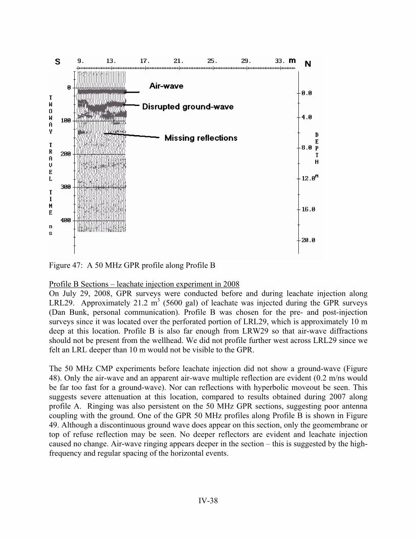
IV-38

Figure 47: A 50 MHz GPR profile along Profile B Profile B Sections – leachate injection experiment in 2008 On July 29, 2008, GPR surveys were conducted before and during leachate injection along LRL29. Approximately 21.2 m3 (5600 gal) of leachate was injected during the GPR surveys (Dan Bunk, personal communication). Profile B was chosen for the pre- and post-injection surveys since it was located over the perforated portion of LRL29, which is approximately 10 m deep at this location. Profile B is also far enough from LRW29 so that air-wave diffractions should not be present from the wellhead. We did not profile further west across LRL29 since we felt an LRL deeper than 10 m would not be visible to the GPR. The 50 MHz CMP experiments before leachate injection did not show a ground-wave (Figure 48). Only the air-wave and an apparent air-wave multiple reflection are evident (0.2 m/ns would be far too fast for a ground-wave). Nor can reflections with hyperbolic moveout be seen. This suggests severe attenuation at this location, compared to results obtained during 2007 along profile A. Ringing was also persistent on the 50 MHz GPR sections, suggesting poor antenna coupling with the ground. One of the GPR 50 MHz profiles along Profile B is shown in Figure 49. Although a discontinuous ground wave does appear on this section, only the geomembrane or top of refuse reflection may be seen. No deeper reflectors are evident and leachate injection caused no change. Air-wave ringing appears deeper in the section – this is suggested by the high-frequency and regular spacing of the horizontal events.

IV-39

Figure 48: GPR CMP survey with 50 MHz antennas, along profile B approximately 10 m south of LRL29 The 25 MHz profiles also showed no change with leachate injection. At least one prominent subsurface feature was identified, however, on the 25 MHz sections: a strong diffraction at lateral position approximately 7.6 m (Figure 50). The diffraction hyperbola was fit with a synthetic hyperbola to estimate GPR wave velocity and depth of the diffracting object at this location (Figure 51). The hyperbola suggests a buried object at about 2.2 m depth, approximately 7.5 m along the GPR line. The velocity at this location is about 0.05 m/ns, significantly lower than the velocity obtained along profile A. This slow velocity, obtained from diffraction hyperbola fitting, also assures us that this diffraction is not from an above-ground source. Figure 50 shows a prominent reflector, or multiple of the air-, ground-wave couplet at about 160-200 ns (depth 3-5 m). We are not certain what this feature is. If real, it could be a temporary cover layer within the refuse. Figure 51 shows that fitting the hyperbola along Profile B (25 MHz) reveals a velocity of 0.05 m/ns. The depth to the top of the hyperbola is at 2.24 m depth.

IV-40

Figure 49: Pre-injection profile across LRL29 with the 50 MHz GPR antennas

Figure 50: GPR section with 25 MHz antennas across profile B. Note the diffraction approximately 7.5 north of the south end of the line

IV-41

Figure 51: Hyperbola fit to data obtained post-subsidence at line 2 Profile C Section – 50 MHz antenna One profile was obtained over LRL28 during the summer of 2007. The depth of LRL28 should be about 5 m at this location. This profile is shown in Figures 52, 53, and 54 using different plotting parameters. LRL28 appears to be visible as a very faint diffraction. No distinct reflections are visible below LRL28. The diffraction associated with LRL28 along Profile C exhibits a faintly visible hyperbolic shape, allowing it to be fit with an idealized diffraction to assess subsurface velocity. Several attempts to “fit” this diffraction reveal a velocity of about 0.05 m/ns. This is considerably lower than that obtained from the CMP survey, which only imaged the cover and possibly upper refuse layer. Thus the GPR wave velocity in the refuse may decrease with depth, perhaps indicating more moisture deeper in the landfill, or more degraded waste. Interestingly, a velocity of 0.05 m/ns also was obtained from a diffraction hyperbola for a shallower diffraction imaged by the 25 MHz antennas along Profile B.

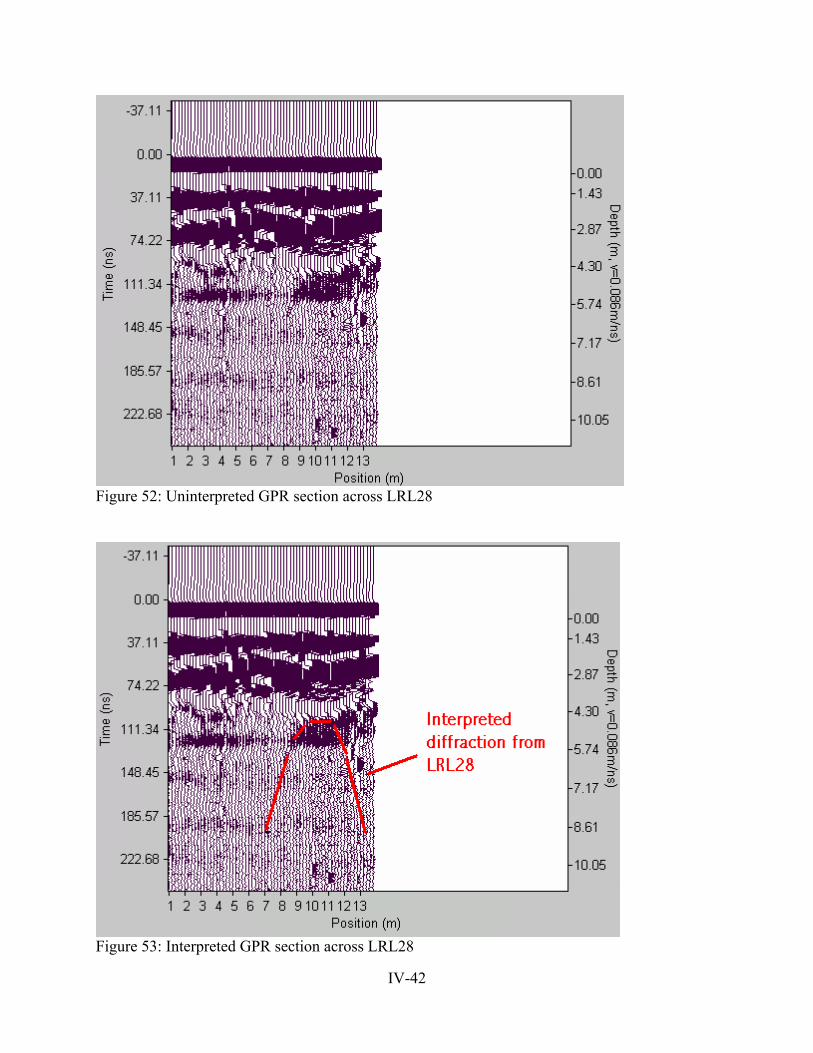
IV-42

Figure 52: Uninterpreted GPR section across LRL28

Figure 53: Interpreted GPR section across LRL28

IV-43

Figure 54: Color display of GPR survey across LRL28 2.5 GPR Conclusions This experiment showed that ground-penetrating radar (GPR) surveys are useful for imaging the interiors of bioreactor landfill cells. We found the optimum antenna frequency to be 50 MHz since the 100 MHz antenna has too shallow a penetration depth, whereas the 25 MHz antenna, while did not achieve better depth penetration, has low resolution, and is cumbersome to use in the field. The average radar wave velocity for the cover and topmost refuse varies from 0.05 to 0.086 m/ns. GPR wave velocity appears to decrease with depth, perhaps reflecting an increase in moisture content. The GPR system is capable of imaging the LRLs at a depth of about 4.5 m. No definite reflections could be identified below this depth. Specifically, GPR profiling showed that: (1) Profiles with 100 MHz antennas only imaged the top of the refuse as a strong reflection that was somewhat irregular. The relatively high frequency 100 MHz signal could not penetrate deeper than about 2.5 m.

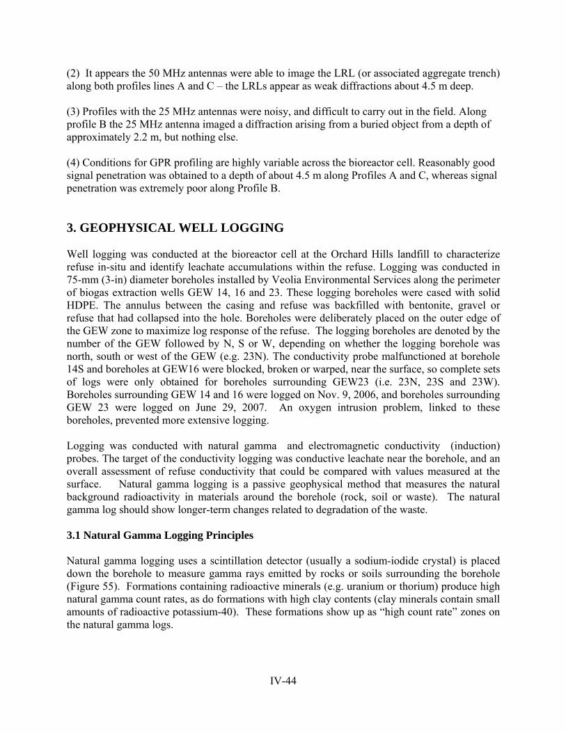
IV-44

(2) It appears the 50 MHz antennas were able to image the LRL (or associated aggregate trench) along both profiles lines A and C – the LRLs appear as weak diffractions about 4.5 m deep. (3) Profiles with the 25 MHz antennas were noisy, and difficult to carry out in the field. Along profile B the 25 MHz antenna imaged a diffraction arising from a buried object from a depth of approximately 2.2 m, but nothing else. (4) Conditions for GPR profiling are highly variable across the bioreactor cell. Reasonably good signal penetration was obtained to a depth of about 4.5 m along Profiles A and C, whereas signal penetration was extremely poor along Profile B. 3. GEOPHYSICAL WELL LOGGING Well logging was conducted at the bioreactor cell at the Orchard Hills landfill to characterize refuse in-situ and identify leachate accumulations within the refuse. Logging was conducted in 75-mm (3-in) diameter boreholes installed by Veolia Environmental Services along the perimeter of biogas extraction wells GEW 14, 16 and 23. These logging boreholes were cased with solid HDPE. The annulus between the casing and refuse was backfilled with bentonite, gravel or refuse that had collapsed into the hole. Boreholes were deliberately placed on the outer edge of the GEW zone to maximize log response of the refuse. The logging boreholes are denoted by the number of the GEW followed by N, S or W, depending on whether the logging borehole was north, south or west of the GEW (e.g. 23N). The conductivity probe malfunctioned at borehole 14S and boreholes at GEW16 were blocked, broken or warped, near the surface, so complete sets of logs were only obtained for boreholes surrounding GEW23 (i.e. 23N, 23S and 23W). Boreholes surrounding GEW 14 and 16 were logged on Nov. 9, 2006, and boreholes surrounding GEW 23 were logged on June 29, 2007. An oxygen intrusion problem, linked to these boreholes, prevented more extensive logging. Logging was conducted with natural gamma and electromagnetic conductivity (induction) probes. The target of the conductivity logging was conductive leachate near the borehole, and an overall assessment of refuse conductivity that could be compared with values measured at the surface. Natural gamma logging is a passive geophysical method that measures the natural background radioactivity in materials around the borehole (rock, soil or waste). The natural gamma log should show longer-term changes related to degradation of the waste. 3.1 Natural Gamma Logging Principles Natural gamma logging uses a scintillation detector (usually a sodium-iodide crystal) is placed down the borehole to measure gamma rays emitted by rocks or soils surrounding the borehole (Figure 55). Formations containing radioactive minerals (e.g. uranium or thorium) produce high natural gamma count rates, as do formations with high clay contents (clay minerals contain small amounts of radioactive potassium-40). These formations show up as “high count rate” zones on the natural gamma logs.

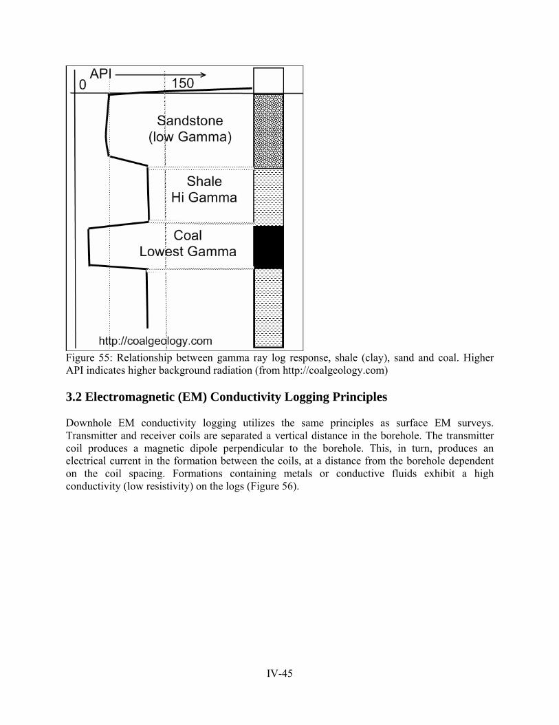
IV-45

Figure 55: Relationship between gamma ray log response, shale (clay), sand and coal. Higher API indicates higher background radiation (from http://coalgeology.com) 3.2 Electromagnetic (EM) Conductivity Logging Principles Downhole EM conductivity logging utilizes the same principles as surface EM surveys. Transmitter and receiver coils are separated a vertical distance in the borehole. The transmitter coil produces a magnetic dipole perpendicular to the borehole. This, in turn, produces an electrical current in the formation between the coils, at a distance from the borehole dependent on the coil spacing. Formations containing metals or conductive fluids exhibit a high conductivity (low resistivity) on the logs (Figure 56).

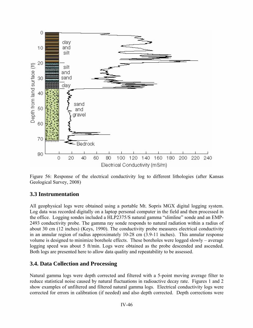
IV-46

Figure 56: Response of the electrical conductivity log to different lithologies (after Kansas Geological Survey, 2008) 3.3 Instrumentation All geophysical logs were obtained using a portable Mt. Sopris MGX digital logging system. Log data was recorded digitally on a laptop personal computer in the field and then processed in the office. Logging sondes included a HLP2375/S natural gamma “slimline” sonde and an EMP-2493 conductivity probe. The gamma ray sonde responds to natural radiation within a radius of about 30 cm (12 inches) (Keys, 1990). The conductivity probe measures electrical conductivity in an annular region of radius approximately 10-28 cm (3.9-11 inches). This annular response volume is designed to minimize borehole effects. These boreholes were logged slowly – average logging speed was about 5 ft/min. Logs were obtained as the probe descended and ascended. Both logs are presented here to allow data quality and repeatability to be assessed. 3.4. Data Collection and Processing Natural gamma logs were depth corrected and filtered with a 5-point moving average filter to reduce statistical noise caused by natural fluctuations in radioactive decay rate. Figures 1 and 2 show examples of unfiltered and filtered natural gamma logs. Electrical conductivity logs were corrected for errors in calibration (if needed) and also depth corrected. Depth corrections were

IV-47

required since well logging started when the cable head was at the ground surface. This was originally recorded as “zero depth” in the raw data. The actual logging depth, however, is the depth of the sensor below ground surface (bgs). The natural gamma sensor is 3.5 ft below the cable head and the EM conductivity sensor is 3.31 ft below the cable head. So all log data values had to be shifted deeper by these amounts. These are also the minimum depths that may be logged. None of the holes were logged to their complete depth. In all cases obstructions and/or bent casing was encountered by the logging tool, typically about 10 ft above the bottom of the holes, or, in the case of GEW16, just below the surface.

Figure 57: Raw natural gamma log Figure 58: Processed log 3.5 Natural Gamma Log Interpretation Processed natural gamma logs are displayed in the figures that follow. On the left is the log obtained with the natural gamma sonde (NGS) descending down the borehole. On the right is the log obtained as the sonde ascends the borehole. “Real” features should appear on both logs. The natural gamma logs are remarkably similar, as shown in Figures 56 through 63. All natural gamma logs recorded at the bioreactor cell exhibit a high count rate in the upper 10-12 ft and a very low count rate below this. My interpretation is that a bentonite seal is filling the annulus between the casing and refuse in the upper 10-12 ft and, below this, the annulus is largely filled with gravel to the bottom of the well. Count rates below 30 cps (counts-per-second) are typical of dolomitic gravel (Bleuer, 2004). Thus, the natural gamma logs appear to be predominantly responding to the gravel and little else. Variations in the count rate may be due to slightly more

14S down processed

0 10 20 30 40 50 60 70 80

010

2030

4050

6070

Depth B

GS (ft)

Natural gamma (cps)

14S down -- raw

data

0 10 20 30 40 50 60 70 80 90

100

010

2030

4050

6070

Depth (ft)

Natural gamma (cps)

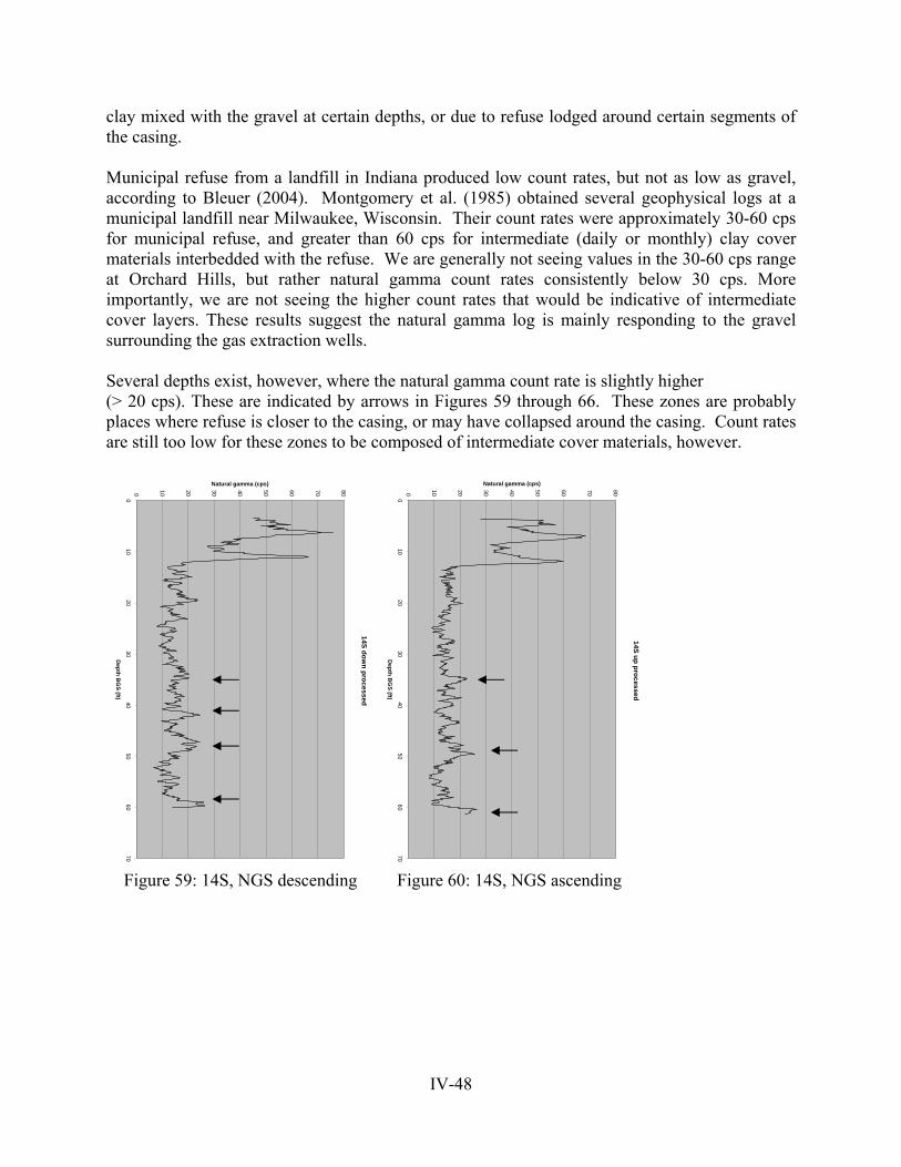
IV-48

clay mixed with the gravel at certain depths, or due to refuse lodged around certain segments of the casing. Municipal refuse from a landfill in Indiana produced low count rates, but not as low as gravel, according to Bleuer (2004). Montgomery et al. (1985) obtained several geophysical logs at a municipal landfill near Milwaukee, Wisconsin. Their count rates were approximately 30-60 cps for municipal refuse, and greater than 60 cps for intermediate (daily or monthly) clay cover materials interbedded with the refuse. We are generally not seeing values in the 30-60 cps range at Orchard Hills, but rather natural gamma count rates consistently below 30 cps. More importantly, we are not seeing the higher count rates that would be indicative of intermediate cover layers. These results suggest the natural gamma log is mainly responding to the gravel surrounding the gas extraction wells. Several depths exist, however, where the natural gamma count rate is slightly higher (> 20 cps). These are indicated by arrows in Figures 59 through 66. These zones are probably places where refuse is closer to the casing, or may have collapsed around the casing. Count rates are still too low for these zones to be composed of intermediate cover materials, however.

Figure 59: 14S, NGS descending Figure 60: 14S, NGS ascending

14S up processed

0 10 20 30 40 50 60 70 80

010

2030

4050

6070

Depth B

GS (ft)

Natural gamma (cps)

14S down processed

0 10 20 30 40 50 60 70 80

010

2030

4050

6070

Depth B

GS (ft)

Natural gamma (cps)

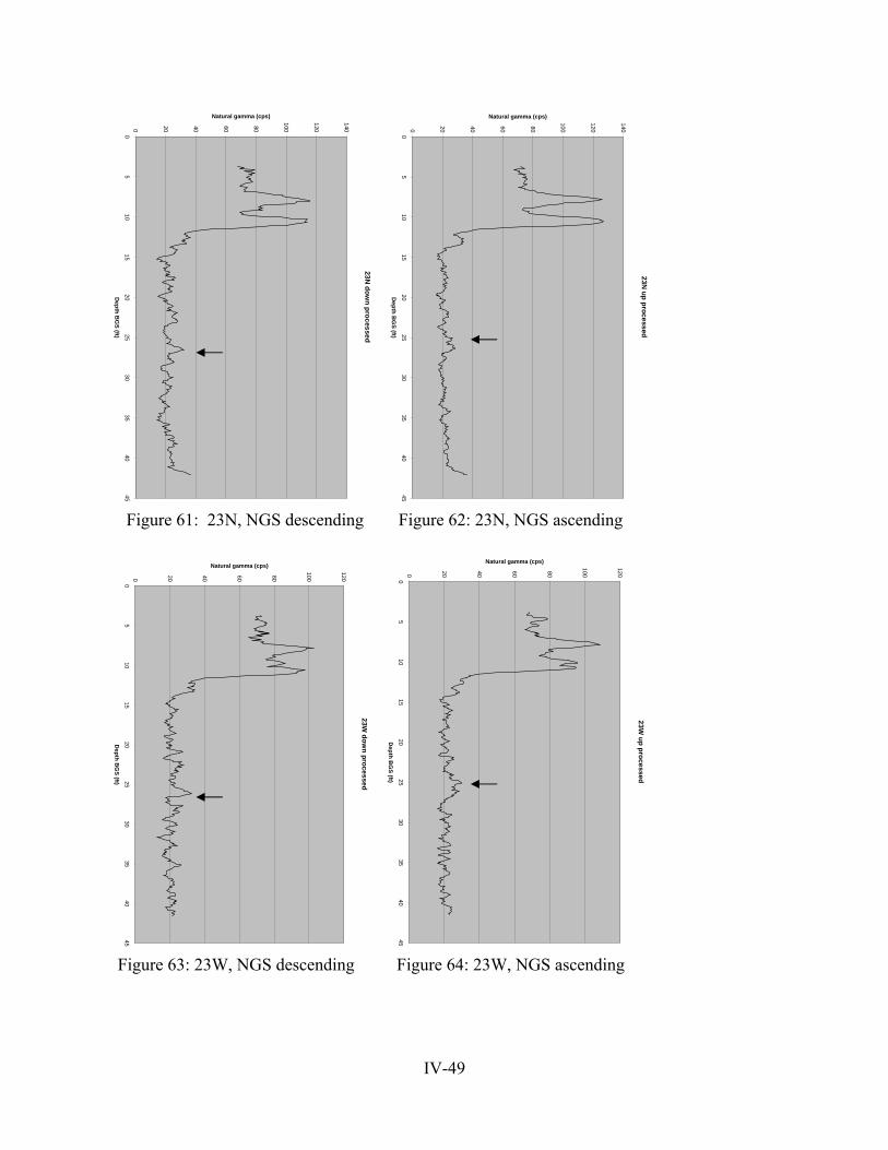
IV-49

Figure 61: 23N, NGS descending Figure 62: 23N, NGS ascending

Figure 63: 23W, NGS descending Figure 64: 23W, NGS ascending

23N up processed

0 20 40 60 80

100

120

140

05

1015

2025

3035

4045

Depth B

GS (ft)

Natural gamma (cps)

23W up processed

0 20 40 60 80

100

120

05

1015

2025

3035

4045

Depth B

GS (ft)

Natural gamma (cps)

23N dow

n processed

0 20 40 60 80

100

120

140

05

1015

2025

3035

4045

Depth B

GS (ft)

Natural gamma (cps)

23W dow

n processed

0 20 40 60 80

100

120

05

1015

2025

3035

4045

Depth B

GS (ft)

Natural gamma (cps)

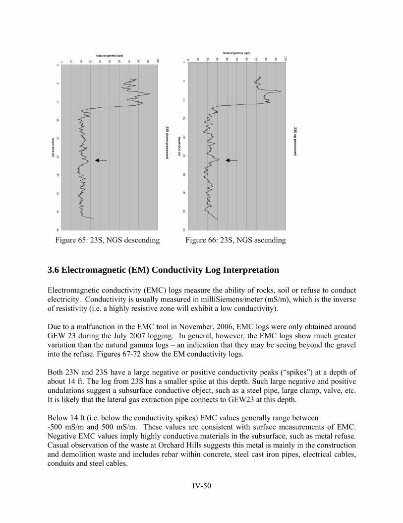
IV-50

Figure 65: 23S, NGS descending Figure 66: 23S, NGS ascending 3.6 Electromagnetic (EM) Conductivity Log Interpretation Electromagnetic conductivity (EMC) logs measure the ability of rocks, soil or refuse to conduct electricity. Conductivity is usually measured in milliSiemens/meter (mS/m), which is the inverse of resistivity (i.e. a highly resistive zone will exhibit a low conductivity). Due to a malfunction in the EMC tool in November, 2006, EMC logs were only obtained around GEW 23 during the July 2007 logging. In general, however, the EMC logs show much greater variation than the natural gamma logs – an indication that they may be seeing beyond the gravel into the refuse. Figures 67-72 show the EM conductivity logs. Both 23N and 23S have a large negative or positive conductivity peaks (“spikes”) at a depth of about 14 ft. The log from 23S has a smaller spike at this depth. Such large negative and positive undulations suggest a subsurface conductive object, such as a steel pipe, large clamp, valve, etc. It is likely that the lateral gas extraction pipe connects to GEW23 at this depth. Below 14 ft (i.e. below the conductivity spikes) EMC values generally range between -500 mS/m and 500 mS/m. These values are consistent with surface measurements of EMC. Negative EMC values imply highly conductive materials in the subsurface, such as metal refuse. Casual observation of the waste at Orchard Hills suggests this metal is mainly in the construction and demolition waste and includes rebar within concrete, steel cast iron pipes, electrical cables, conduits and steel cables.

23S down processed

0 10 20 30 40 50 60 70 80 90

100

05

1015

2025

3035

4045

Depth B

GS (ft)

Natural gamma (cps)

23S up processed

0 10 20 30 40 50 60 70 80 90

100

05

1015

2025

3035

4045

Depth B

GS (ft)

Natural gamma (cps)

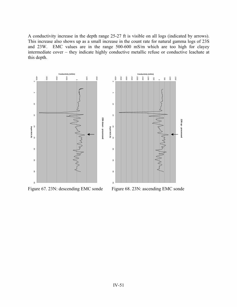
IV-51

A conductivity increase in the depth range 25-27 ft is visible on all logs (indicated by arrows). This increase also shows up as a small increase in the count rate for natural gamma logs of 23S and 23W. EMC values are in the range 500-600 mS/m which are too high for clayey intermediate cover – they indicate highly conductive metallic refuse or conductive leachate at this depth.

Figure 67. 23N: descending EMC sonde Figure 68. 23N: ascending EMC sonde

23N up - processed

-4000

-3500

-3000

-2500

-2000

-1500

-1000

-500 0

500

1000

1500

05

1015

2025

3035

4045

Depth B

GS (ft)

Conductivity (mS/m)

23N dow

n - processed

-4000

-3000

-2000

-1000 0

1000

2000

05

1015

2025

3035

4045

Depth B

GS (ft)

Conductivity (mS/m)

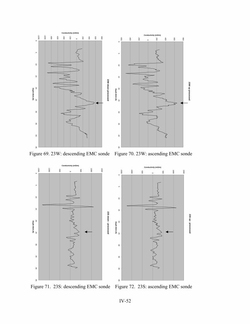
IV-52

Figure 69. 23W: descending EMC sonde Figure 70. 23W: ascending EMC sonde

Figure 71. 23S: descending EMC sonde Figure 72. 23S: ascending EMC sonde

23S up - processed

-1500

-1000

-500 0

500

1000

1500

05

1015

2025

3035

4045

Depth B

GS (ft)

Conductivity (mS/m)

23W dow

n processed

-1200

-1000

-800

-600

-400

-200 0

200

400

600

800

05

1015

2025

3035

4045

Depth B

GS (ft)

Conductivity (mS/m)

23W up processed

-600

-400

-200 0

200

400

600

800

05

1015

2025

3035

4045

Depth B

GS (ft)

Conductivity (mS/m)

23S down - processed

-1500

-1000

-500 0

500

1000

1500

05

1015

2025

3035

4045

Depth B

GS (ft)

Conductivity (mS/m)

IV-53

3.7 Logging Conclusions Natural gamma and electromagnetic conductivity logs were obtained from boreholes surrounding GEW14 and GEW23. The following conclusions may be drawn: (1) Natural gamma logs are mainly sensing the bentonite seal in the upper 12 ft (3.7 m) and gravel backfill below this. At a few depths where count rates are slightly higher (20-30 cps) refuse apparently surrounds or is in close proximity to the boreholes. These higher count rates could also be explained by small amounts of clay mixed in with the gravel. (2) Electromagnetic conductivity logs obtained in boreholes surrounding GEW23 indicate metal hardware, possibly related to a connection at a depth of about 14 ft (4.27 m) bgs. (3) Increased conductivity at 24-26 ft (7.32-7.93 m) bgs suggests conductive refuse or an accumulation of leachate at this depth. Logging before and after leachate injection would clarify which conductive zones were due to leachate (if any) and which were due to buried metallic waste. Neutron logging would be extremely useful in that it could determine the moisture content of the waste. Gamma-gamma density logging would also be extremely useful in showing the densification of waste with depth (and degradation), as well as providing in-situ density values for interpretation of seismic survey data and geotechnical modeling. 4. CONCLUSIONS EM: Surveys with coils spaced 10 and 20 m recorded repeatable conductivity increases associated with leachate injection along LRL29. Non-uniform injection is suggested by the EM conductivity distributions. Coils with spacings less than 10 m did not respond to leachate injection. Lines crossing LRL28 and LRL29 also did not show conductivity changes changes with leachate injection. EM surveys, in the future, could be conducted over LRLs to assess the effectiveness of injection, however, quantitative interpretation of EM data is difficult. Assessing the volume of injection, leachate migration distances, etc. requires modeling of the EM data which is very time-consuming and typically produces non-unique solutions. GPR: The 50 and 25-MHz antennas imaged subsurface features to a maximum depth of 8 m. LRL 28 (and its associated trench) was imaged with a 50 MHz GPR profile. Other prominent subsurface reflectors were imaged, but their origin is unknown. LRL 29, at depth 10 m, was generally beneath the depth of the GPR penetration – thus leachate injection along LRL29 could not be observed. Well logging: The geophysical well logs appear to be strongly influenced by well construction, including bentonite seals and gravel packs surrounding the gas extraction wells. Little to no useful information was obtained. Advanced processing of these logs may reveal additonal information. For example, two logs may be subtracted, or divided, to eliminate the effect of the

IV-54

gravel. Electical conductivity logs appeared to measure conductivity values similar to those recorded on the surface. CITED REFERENCES Annan, A.P. and S.W. Cosway, 1992, Ground penetrating radar design: in Proceedings of the

Symposium on the Application of Geophysics to Engineering and Environmental Problems, Environmental and Engineering Geophysical Society, Wheat Ridge, CO, p. 271-280.

Bleuer, N.K., 2004, Slow-logging subtle sequences the gamma-ray log character of glacigenic and other unconsolidated sedimentary sequences: Indiana Geological Survey Special Report 65, 39 p.

Butcher, A.P. and W.S.A. Tam, 1997, The use of Rayleigh waves to detect the depth of a shallow landfill, from McCann: in Fenning and Reeves (eds.), Modern Geophysics in Engineering Geology, Geol. Soc. Engr. Geol. Special Publication No. 12, p. 97-102.

Carpenter, P.J., Doll, W.E., and R.D. Kaufmann, 1995, Geophysical surveys over karst features near the Oak Ridge Y-12 Plant, Oak Ridge, Tennessee: Oak Ridge Y-12 Plant Report Y/ER-200, Lockeed Martin Energy Systems, Inc.

Carpenter, P.J., Doll, W.E., and R.D. Kaufmann, 1998, Geophysical character of buried sinkholes on the Oak Ridge Reservation, Tennessee: Journal of Environmental and Engineering Geophysics, v. 3, p. 133-145.

Davis, J.J. and A.P. Annan, 1989. Ground penetrating radar for high-resolution mapping of soil and rock stratigraphy: Geophysical Prospecting, v. 37, 531-551.

Dobrin, M.B., 1981 and S.H. Savit, 1988, Introduction to Geophysical Prospecting, 4th Edition, McGraw-Hill, New York.

GeoTom, 2008, GeoTomCG, Three-dimensional seismic-tomography manual, GeoTom, LLC, Apple Valley, MN, 71 p.

Grellier, S., Reddy, K.R., Carpenter, P.J., Bogner J.E., and J. Gangathulasi, 2007, Leachate distribution and geotechnical stability of bioreactor landfills: Progress Report, August, 2005 – January, 2007, University of Illinois at Chicago, Department of Civil and Materials Engineering, Chicago, IL, 272 p.

Haker, C.D., G.J. Rix, and C.G. Lai, 1997, Dynamic properties of municipal solid waste landfills from surface waves: in Proceedings of the Symposium on the Application of Geophysics to Engineering and Environmental Problems, Environmental and Engineering Geophysical Society, Wheat Ridge, CO, 10 p.

Keys, W.S., 1990, Borehole Geophysics Applied to Ground-water Investigations: Techniques of Water-Resources Investigations of the U.S. Geological Survey, Book 2, Chapter E2, U.S. Govt. Printing Office, Denver, CO, 150 p.

Lytle, R.J, K.A. Dines, E.F. Laine, and D.L. Lager., 1978, Electromagnetic Cross-Borehole Survey of a Site Proposed for an Urban Transit Station: UCRL-52484, Lawrence Livermore Laboratory, University of California, 19 p.

McNeill, J.D., 1980, Electromagnetic terrain conductivity measurement at low induction numbers: Geonics, Ltd. Technical Note 6, Geonics Ltd, Mississauga, Ontario, 15 p.

Montgomery, R.J., Wierman, D.A., Taylor, R.W., and H.A. Koch, 1985, Use of downhole geophysical methods in determining the internal structure of a large landfill: in Nielsen,

IV-55

D.M., editor, NWWA Conference on Surface and Borehole Geophysical Methods in Ground Water Investigations, National Water Well Association, Worthington, OH, p. 377-385.

Mt. Sopris Instrument Co., Inc., 2002, 2PIA-1000 Poly Induction Probe: Technical Manual, P/N 70000177B, Mt. Sopris Instruments Co, Golden, CO, 19 p.

Pakiser, L.C. and R.A. Black, 1957, Exploring for Ancient Channels with the Refraction Seismograph: Geophysics, v. 22, no. 1, p. 32-47.

Park, C.B., R.D. Miller, and J. Xia, 1999, Multichannel analysis of surface waves: Geophysics, v. 64, no. 3, p. 800–808.

Park, C.B., R.D. Miller, and H. Miura, 2002, Optimum field parameters of a MASW survey [Exp. Abs.]: Soc. Explor. Geophys.-Japan, Tokyo, May 22-23.

Peterson, J. E., B. N. P. Paulson, and T. V. McEvilly, 1985, Applications of Algebraic Reconstruction Techniques to Crosshole Seismic Data: Geophysics, v. 50, p. 1566-1580.

Redpath, B.B., 1973, Seismic Refraction Exploration for Engineering Site Investigations: Technical Report E-73-4, U.S. Army Waterways Experiment Station, Explosive Excavation Research Laboratory, Livermore, California, 51 p.

RIMROCK Geophysics, 1992, SIPT2 Refraction Processing Software, Version 3.2: Rimrock Geophysics, Boulder, Colorado.

Scott, J.H., 1973, Seismic Refraction Modeling by Computer: Geophysics, 38(2):271–284. Scott, J.H., 1977, SIPT — A Seismic Refraction Inverse Modeling Program for Time-Share

Terminal Computer Systems: U.S. Geol. Survey. Open-File Reports 77-366, 27 p. Tweeton, D.R., M.J. Jackson, and K.S. Roessler, 1992, BOMCRATR – A Curved Ray

Tomographic Computer Program for Geophysical Applications: U.S. Bureau of Mines Report of Investigations 9411, 39 p.

geophysical monitoring of leachate recirculation · pdf fileresistivity tomography, ......

Documents