geophysical journal international - geos.ed.ac.uk d. halliday, a. curtis and k. wapenaar to use...

Geophys. J. Int. (2012) 189, 1015–1024 doi: 10.1111/j.1365-246X.2012.05396.x

GJI

Sei

smol

ogy

Generalized PP + PS = SS from seismic interferometry

David Halliday,1 Andrew Curtis2 and Kees Wapenaar3

1Schlumberger Cambridge Research, High Cross, Madingley Road, Cambridge, CB3 0EL, UK. E-mail: [email protected] of GeoSciences, Grant Institute, The University of Edinburgh, Kings Buildings, West Mains Road, Edinburgh EH9 3JW, UK3Department of Geoscience and Engineering, Delft University of Technology, PO Box 5048, 2600 GA Delft, The Netherlands

Accepted 2012 January 20. Received 2012 January 20; in original form 2011 August 31

S U M M A R YPP + PS = SS refers to a method introduced by Grechka and Tsvankin in 2002 that usesrecordings of PP and PS reflections between sources and receivers to estimate the SS reflectionsbetween those same receivers. Using source–receiver seismic interferometry as a basis, wederive new, dynamically correct expressions relating reflected and converted P- and S-waverecordings to both P- and S-wave sources. We use these expressions to derive a generalizedform of relationship between P and S waves, and show that the PP + PS = SS method ofGrechka and co-workers is a special case of these new relationships. By considering the simpleexample of two elastic half-spaces, we illustrate the differences between the special case ofPP + PS = SS and the generalized approach derived here. By relating the method to seismicinterferometry, it is possible to see further applications of the new relationships in acquisitionand processing of P and S waves, and also in the development of new imaging and inversionschemes.

Key words: Interferometry; Controlled source seismology; Body waves; Theoretical seis-mology.

I N T RO D U C T I O N

The shear wave component of the seismic wavefield is important in determining the shear wave velocities in any medium. For example, in theEarth’s subsurface the combination of P- and S-wave information allows fluid and rock properties to be discriminated. It is also particularlyimportant in the study of anisotropic media where the polarizations of fast and slow split S waves are often used to infer the average alignmentof fracture fields, or of crystalline lattice structures such as in uppermost mantle olivine.

In industrial geophysics, typically converted PS responses (P waves propagating down to a reflector at which the wave reflects andconverts to S energy that propagates back to the surface) are used to infer S-wave velocity structure. However, this is undesirable from severalpoints of view: both P- and S-wave velocity models are required to estimate reflection and conversion points, and Grechka & Tsvankin (2002)discuss the difficulty of velocity analysis for converted S waves due to the asymmetric moveout of the PS response. Ideally, pure PP responses(i.e. P-wave source, P-wave receiver) and pure SS responses (S-wave source, S-wave receiver) would be analysed independently.

Typically, the horizontal components of a three-component geophone are assumed to predominantly contain S waves whereas the verticalcomponent is assumed to contain P waves. There are also various separation techniques that can be used to make more accurate measurementsof the recorded P- and S-wavefields. For example, Curtis & Robertsson (2002) and Robertsson & Curtis (2002) introduce methods to separateP- and S-wave recordings using distributed arrays of three-component geophones. Sources of P-wave energy are also available as standardindustrial equipment. However, it is far more difficult to inject significant S-wave energy into the ground economically.

Grechka & Tsvankin (2002) and Grechka & Dewangan (2003) proposed a potential solution to this problem: by combining PP and PSresponses, pseudo-shear wave data can be generated that has the same kinematics as a pure SS response. Presumably, as the interest in elasticfull waveform imaging and inversion grows, the recovery of shear wave velocity profiles, and the study of anisotropic media will come undergreater scrutiny. Therefore, it is important to consider approaches such as that presented by Grechka & Tsvankin (2002) and Grechka &Dewangan (2003).

We examine the relationship between P- and S-wave energy in a novel way using theory from the field of seismic interferometry.Generally, seismic interferometry refers to the process of generating responses to imagined or virtual approximately impulsive sourcesby cross-correlation (Wapenaar 2003; van Manen et al. 2006; Wapenaar & Fokkema 2006), cross-convolution (e.g. Slob et al. 2007) ordeconvolution (e.g. Vasconcelos & Snieder 2008a,b; Wapenaar et al. 2008, 2011) of wavefields from surrounding energy sources recorded atdifferent receiver locations. Recent work has shown that intersource wavefields can be estimated by cross-correlating recordings of a pair ofsources at a range of azimuths (Hong & Menke 2006; Curtis et al. 2009). Furthermore, Curtis & Halliday (2010) demonstrated that it is possible

C© 2012 The Authors 1015Geophysical Journal International C© 2012 RAS

Geophysical Journal International

1016 D. Halliday, A. Curtis and K. Wapenaar

to use so-called source–receiver interferometry to estimate the wavefield between a source and a receiver, allowing interferometry to be usedto construct wavefields between any combination of source and receiver pairs. Halliday & Curtis (2010) also showed that the source–receiverrelationships establish a direct link between seismic interferometry and seismic imaging. These theorems are generalized forms of existingimaging methods, for example, the methods of Oristaglio (1989) and Vasconcelos et al. (2010). Most generally, interferometry can be thoughtof as a method to synthesize desired wavefields that were not directly recorded. An example of such a wavefield is the SS response describedearlier.

In this paper, we extend the applicability of the new source–receiver relationships by using the results of Curtis & Halliday (2010) tofind interferometric relationships that describe precisely how P- and S-wave responses between sources and receivers are related. Wapenaar& Fokkema (2006) have already shown how P- and S-wave source and receivers can be incorporated within the framework for interferometryprovided by reciprocity theorems of the correlation type, and the derivation in this paper follows a similar path to theirs. As a result, wederive the PP + PS = SS equation of Grechka & Dewangan (2003) from source–receiver interferometry. Although the derivation of Grechka& Dewangan (2003) was in part heuristic and was purely kinematic, here we show that this can also be derived from first principles. Thesource–receiver representations that we consider are derived dynamically, directly from reciprocity and representation theorems (Curtis &Halliday 2010). This approach reveals the key approximations and assumptions inherent in the approach of Grechka & Tsvankin (2002)and Grechka & Dewangan (2003), and provides a theoretical framework to develop future P- and S-wave processing, imaging and inversionalgorithms, potentially using novel combinations of P- and S-wave energy sources and receivers.

At the time of writing, there are already a range of applications that apply the single integral (virtual-source or virtual-receiver) forms ofseismic interferometry using P and S waves. For example, Gaiser & Vasconcelos (2010) apply interferometry to seabed data to recover PP,PS and (potentially) SS responses, Bakulin & Mateeva (2008) apply seismic interferometry to horizontal component borehole geophones tocreate virtual-shear wave check shots, Miyazawa et al. (2008) apply seismic interferometry to ambient noise recorded in a borehole and showthat they can observe shear wave splitting on the resultant virtual-source records, and van der Neut et al. (2011) outline a theoretical frameworkfor the application of multidimensional deconvolution using separated P and S waves. Tonegawa & Nishida (2010) study earthquake recordsand show that virtual-receiver seismic interferometry (Curtis et al. 2009) can be used to recover direct P and S waves propagating betweenpairs of deep earthquakes. While an application of the (double-integral) form of source–receiver interferometry that differentiates P and Swaves has yet to be published, here we will demonstrate that the PP + PS = SS method may be considered as such an application. Moreover,the relationships derived here provide a framework for the development of future applications of source–receiver interferometry using P- andS-wave sources and receivers.

First, we consider the derivation of source–receiver interferometric relationships for P- and S-wave sources and receivers. We illustratethat in the general case, with a source and receiver located within two enclosing boundaries, the recovery of the SS reflection response throughinterferometry alone (i.e. without recording it directly) in a simple example requires only S-wave sources and S-wave receivers. Then, weintroduce the approximations and assumptions required to derive the special case of PP + PS = SS published by Grechka & Dewangan(2003). In this special case, contrary to the general case, no S-wave sources are required. Using the same simple model, we illustrate thekey differences between the PP + PS = SS approach, and this general approach based on the new representations derived here. Finally, wediscuss further applications of the source–receiver integrals for P and S waves.

S O U RC E – R E C E I V E R R E P R E S E N TAT I O N F O R P A N D S WAV E S

We now derive the source–receiver representations for P and S waves by following the approach of Curtis & Halliday (2010, appendix A).In the following, we will also take advantage of the P- and S-wave Green’s functions used by Wapenaar & Haime (1990) and Wapenaar &Fokkema (2006).

Using the elastodynamic representation theorem, Curtis & Halliday (2010, appendix A) show that the response between a real sourceand a real receiver in a lossless inhomogeneous anisotropic medium can be derived using two correlation-type representation theorems.

Gqm(x2, x1) − G∗qm(x2, x1) =

∫S

{G∗

qn(x2, x)n j cnjkl∂k�ml (x1, x) − n j cnjkl∂k G∗ql (x2, x)�mn(x1, x)

}dS, (1)

where

�ml (x1, x) = −∫

S′

{Gn′l (x

′, x)n j ′ cn′ j ′k′l ′∂k′ G∗l ′m(x′, x1) − n j ′ cn′ j ′k′l ′∂k′ Gl ′l (x

′, x)G∗n′m(x′, x1)

}dS′. (2)

Here, Gqm(x2,x1) is the Green’s function in the frequency domain representing the qth component of particle displacement at x2 due to aunidirectional point force in the m-direction at x1, nj is the jth component of the normal vector on the boundary S, ∂k denotes a spatialderivative in the k-direction and cnjkl is the stiffness tensor. Primed and unprimed quantities indicate that these relate to the primed andunprimed boundaries, respectively (Fig. 1a), and Einstein’s summation principle for repeated indices applies throughout.

Eq. (1) describes the recovery of a Green’s function (plus its time reverse due to the complex conjugate on the left-hand side) between asource at x1 and a receiver at x2 in elastic media, using only Green’s functions from x1 to a surrounding boundary S′ of receivers, and Green’sfunctions from a surrounding boundary S (Fig. 1a). The integral in eq. (2) describes a first step where the boundary S′ is used to determinethe Green’s functions (plus the time reverse) between the source at x1 and each source on the boundary S; hence, this first step turns thesource x1 into a virtual receiver. In a second step, the boundary S is used to determine the Green’s function between the receiver at x2 and

C© 2012 The Authors, GJI, 189, 1015–1024

Geophysical Journal International C© 2012 RAS

PP + PS = SS from seismic interferometry 1017

Figure 1. Canonical geometries for source–receiver interferometry for (a) the correlation–correlation, (b) the correlation–convolution, and (c) theconvolution–convolution forms (Curtis & Halliday 2010). Note the different positions of x1 and x2 relative to the boundaries.

the newly generated virtual receiver x1 (in reality, a source). Thus, this interferometric integral uses both surrounding sources and receiversto reconstruct virtual-source to virtual-receiver wavefields. This specific form of the integral is derived by combining two representationtheorems of the correlation type and can be used in the canonical geometry represented in Fig. 1(a) where the source and receiver both liewithin both boundaries. Figs 1(b) and (c) show other configurations that can be derived using (b) both correlation- and convolution-typerepresentation theorems, and (c) two convolution-type representation theorems, respectively (Curtis & Halliday 2010).

To extend eq. (1) to describe the recovery of P and S responses, we recall from Wapenaar & Fokkema (2006) that the P- and S-wavecomponents of the wavefield can be expressed as a sum of partial derivatives of the displacement

Gψ0m(x2, x1) = −ρc2P∂q Gqm(x2, x1), (3)

Gψk m(x2, x1) = ρc2Sεk jq∂ j Gqm(x2, x1), (4)

where cS is the local S-wave velocity at x2, cP is the local P-wave velocity at x2, ρ is the density at x2, ω is the angular frequency, Gψk m(x2, x1)is the Green’s function representing the S wave at x2 polarized in the plane with normal nk, due to a point force in the m-direction at x1 andGψ0m(x2, x1) is the equivalent Green’s function for a P wave at x2. εkjq is the alternating tensor with ε123 = ε312 = ε231 = −ε213 = −ε321 =−ε132 = 1. When we interpret eqs (3) and (4) as P- and S-wave Green’s functions, we assume that the medium is homogeneous and isotropiclocally around the receiver point, x2. In the following, we will use one notation for the Green’s function, GψK m(x2, x1), with K equal to 0, 1,2 or 3. K = 0 denotes P waves (cf. eq. 3) and K = 1, 2 or 3 denotes a shear wave polarized in the plane with normal nK (cf. eq. 4), assumingappropriate P or S velocities are used.

Eqs (3) and (4) are weighted sums of the spatial derivatives of point-force responses (and likewise, by reciprocity, we can find similarexpressions for the particle displacement due to P- and S-wave sources—see Wapenaar & Fokkema (2006)). Hence, eqs (3) and (4) showhow appropriately weighted sums of partial derivatives of eq. (1) represent P- and S-wave source and receiver Green’s functions. Evaluatingthese sums explicitly using eq. (1) results in

GψQψM(x2, x1) − G∗

ψQψM(x2, x1) =

∫S

{G∗

ψQ n(x2, x)n j cnjkl∂k�ψM l (x1, x)− n j cnjkl∂k G∗ψQl (x2, x)�ψM n(x1, x)

}dS, (5)

with

�ψM l (x1, x) = −∫

S′

{Gn′l (x

′, x)n j ′ cn′ j ′k′l ′∂k′ G∗l ′ψM

(x′, x1) − n j ′ cn′ j ′k′l ′∂k′ Gl ′l (x′, x)G∗

n′ψM(x′, x1)

}dS′. (6)

Here, GψQψM(x2, x1) is the Green’s function representing the P- or S-wave component of the wavefield at x2 due to a P- or S-wave source

at x1. Gn′ψM(x′, x1) is the Green’s function representing the n′th component of particle displacement at x′ due to a P- or S-wave source at x1.

On the source component, the uppercase subscript M runs from 0 to 3, with 0 denoting a P-wave source, and 1 to 3 denoting a shear wavesource polarized in the plane with normal nM .

While the left-hand side of eq. (5) now contains only P-to-S, S-to-P, P-to-P or S-to-S Green’s functions, the right-hand side of eq. (5) andalso eq. (6) contain Green’s functions that require particle displacement and unidirectional point forces on the surfaces S′ and S, respectively.We now follow Wapenaar & Fokkema (2006) in changing these to be P- and S-wave receivers or sources. First, we consider the integral ineq. (6): from Wapenaar & Fokkema (2006, equations 72 and 73) we can write

�ψM l (x1, x) = − 2

ρ

∫S′

∂ j ′ Gψ ′K l (x

′, x)G∗ψ ′

K ψM(x′, x1) dS′. (7)

Because we use P- and S-wave quantities on the boundary, we are assuming that the medium at and outside the boundary S′ is homogeneousand isotropic. Applying the same principles to the integral over S such that it consists of only recordings of P- and S-wave sources, we obtain

GψQψM(x2, x1) − G∗

ψQψM(x2, x1) = 4

ρ2

∫S

∫S′

∂ j G∗ψQψK

(x2, x)∂ j ′ Gψ ′K ψK

(x′, x)G∗ψ ′

K ψM(x′, x1)n j ′ n j dS′ dS. (8)

C© 2012 The Authors, GJI, 189, 1015–1024



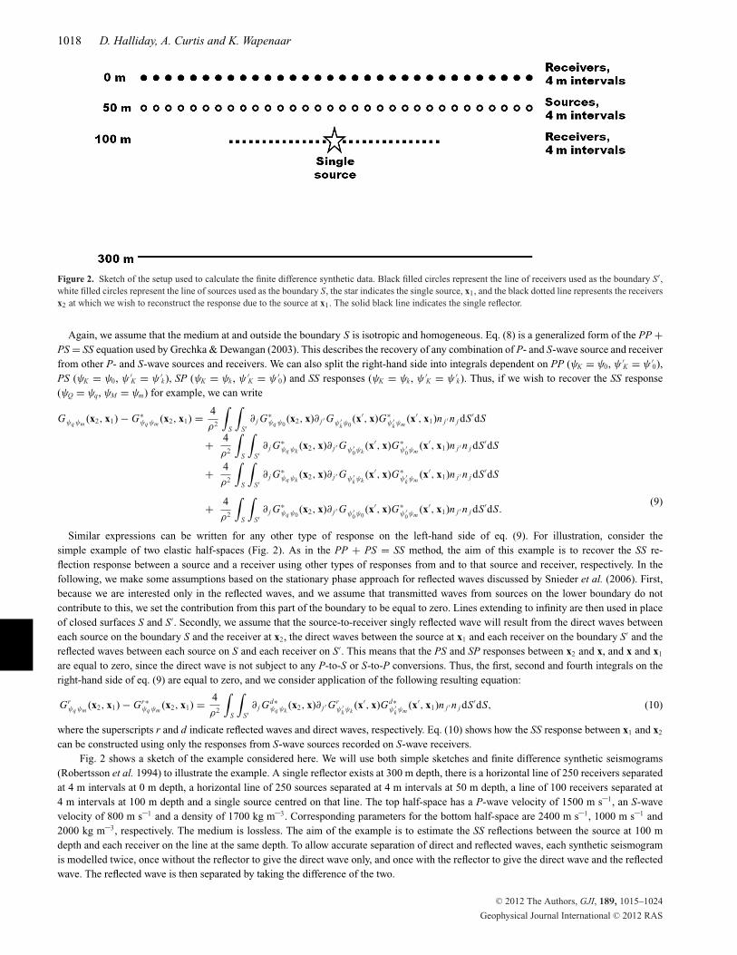
Figure 2. Sketch of the setup used to calculate the finite difference synthetic data. Black filled circles represent the line of receivers used as the boundary S′,white filled circles represent the line of sources used as the boundary S, the star indicates the single source, x1, and the black dotted line represents the receiversx2 at which we wish to reconstruct the response due to the source at x1. The solid black line indicates the single reflector.

Again, we assume that the medium at and outside the boundary S is isotropic and homogeneous. Eq. (8) is a generalized form of the PP +PS = SS equation used by Grechka & Dewangan (2003). This describes the recovery of any combination of P- and S-wave source and receiverfrom other P- and S-wave sources and receivers. We can also split the right-hand side into integrals dependent on PP (ψK = ψ0, ψ ′

K = ψ ′0),

PS (ψK = ψ0, ψ ′K = ψ ′

k), SP (ψK = ψk , ψ ′K = ψ ′

0) and SS responses (ψK = ψk , ψ ′K = ψ ′

k). Thus, if we wish to recover the SS response(ψQ = ψq, ψM = ψm) for example, we can write

Gψq ψm(x2, x1) − G∗

ψq ψm(x2, x1) = 4

ρ2

∫S

∫S′

∂ j G∗ψq ψ0

(x2, x)∂ j ′ Gψ ′kψ0

(x′, x)G∗ψ ′

kψm(x′, x1)n j ′ n j dS′dS

+ 4

ρ2

∫S

∫S′

∂ j G∗ψq ψk

(x2, x)∂ j ′ Gψ ′0ψk

(x′, x)G∗ψ ′

0ψm(x′, x1)n j ′ n j dS′dS

+ 4

ρ2

∫S

∫S′

∂ j G∗ψq ψk

(x2, x)∂ j ′ Gψ ′kψk

(x′, x)G∗ψ ′


+ 4

ρ2

∫S

∫S′

∂ j G∗ψq ψ0

(x2, x)∂ j ′ Gψ ′0ψ0

(x′, x)G∗ψ ′

0ψm(x′, x1)n j ′ n j dS′dS.

(9)

Similar expressions can be written for any other type of response on the left-hand side of eq. (9). For illustration, consider thesimple example of two elastic half-spaces (Fig. 2). As in the PP + PS = SS method, the aim of this example is to recover the SS re-flection response between a source and a receiver using other types of responses from and to that source and receiver, respectively. In thefollowing, we make some assumptions based on the stationary phase approach for reflected waves discussed by Snieder et al. (2006). First,because we are interested only in the reflected waves, and we assume that transmitted waves from sources on the lower boundary do notcontribute to this, we set the contribution from this part of the boundary to be equal to zero. Lines extending to infinity are then used in placeof closed surfaces S and S′. Secondly, we assume that the source-to-receiver singly reflected wave will result from the direct waves betweeneach source on the boundary S and the receiver at x2, the direct waves between the source at x1 and each receiver on the boundary S′ and thereflected waves between each source on S and each receiver on S′. This means that the PS and SP responses between x2 and x, and x and x1

are equal to zero, since the direct wave is not subject to any P-to-S or S-to-P conversions. Thus, the first, second and fourth integrals on theright-hand side of eq. (9) are equal to zero, and we consider application of the following resulting equation:

Grψq ψm

(x2, x1) − Gr∗ψq ψm

(x2, x1) = 4

ρ2

∫S

∫S′

∂ j Gd∗ψq ψk

(x2, x)∂ j ′ Grψ ′

kψk(x′, x)Gd∗

ψ ′kψm

(x′, x1)n j ′ n j dS′dS, (10)

where the superscripts r and d indicate reflected waves and direct waves, respectively. Eq. (10) shows how the SS response between x1 and x2

can be constructed using only the responses from S-wave sources recorded on S-wave receivers.Fig. 2 shows a sketch of the example considered here. We will use both simple sketches and finite difference synthetic seismograms

(Robertsson et al. 1994) to illustrate the example. A single reflector exists at 300 m depth, there is a horizontal line of 250 receivers separatedat 4 m intervals at 0 m depth, a horizontal line of 250 sources separated at 4 m intervals at 50 m depth, a line of 100 receivers separated at4 m intervals at 100 m depth and a single source centred on that line. The top half-space has a P-wave velocity of 1500 m s–1, an S-wavevelocity of 800 m s–1 and a density of 1700 kg m–3. Corresponding parameters for the bottom half-space are 2400 m s–1, 1000 m s–1 and2000 kg m–3, respectively. The medium is lossless. The aim of the example is to estimate the SS reflections between the source at 100 mdepth and each receiver on the line at the same depth. To allow accurate separation of direct and reflected waves, each synthetic seismogramis modelled twice, once without the reflector to give the direct wave only, and once with the reflector to give the direct wave and the reflectedwave. The reflected wave is then separated by taking the difference of the two.

C© 2012 The Authors, GJI, 189, 1015–1024



Figure 3. Sketch example of the kinematics involved in recovering the SS reflection using eq. (10). White circles indicate a line of sources, black circlesindicate a line of receivers, the triangle is a single receiver and the star is a single source. (a) The starting point is the SS reflection between each source onthe boundary S, and each receiver on the boundary S′. (b) The first step is the cross-correlation of the interboundary responses with the direct S wave betweenthe single source and boundary of receivers. The result is the SS reflection between the boundary of sources, and the single source. (c) The second step iscross-correlation of the intersource SS reflections with the direct S wave between the source boundary and the single receiver. This results in the SS reflectionbetween the source and receiver.

Figure 4. (a) SS response between a source on the boundary and the boundary of receivers illustrated in Fig. 3(a). (b) The result of the first cross-correlationstep which gives the SS refection between the source boundary and the single source (Fig. 3b). (c) The result of using source–receiver interferometry to recoverthe SS reflection (Fig. 3c) and (d) the directly modelled SS reflection (accounting for the scale factor introduced in the interferometric estimates).

Fig. 3 shows a number of sketches that illustrate the construction of the unmeasured SS response using eq. (10). Fig. 3(a) shows a sketchof the SS response between a boundary source (white circles), and a boundary receiver (black filled circles). The first pass of interferometry(i.e. solution of the integral over S′ in eq. 10) uses the direct S wave from the boundary of receivers to compute the SS reflection between theboundary of sources and the single source (star). Fig. 3(b) shows this intermediate step, where the part of the ray path between the boundaryof receivers and the single source has been removed (cf. Fig. 3a). The second pass of interferometry (i.e. solution of the integral over S) usesthe direct S wave from the boundary of sources to the single receiver (triangle) to compute the SS reflection between the single receiver andthe source. Fig. 3(c) shows the equivalent sketch, where the part of the ray path between the boundary of sources and the single receiver hasbeen removed, resulting in the reflected wave between the source and the receiver.

Figs 4(a)–(c) show the synthetic data corresponding to the illustrations in Figs 3(a)–(c). These are (a) the SS reflection response betweena single boundary source and each boundary receiver, (b) the intermediate SS reflection response between each boundary source, and thesingle source, (c) the SS reflection response between a source and a line of receivers resulting from eq. (10) and (d) the directly modelled SSreflection response for comparison (right-hand panel). A scale factor is required for the amplitude and phase of panels (c) and (d) to match(the scale factor is due to the source wavelet and implementation of the source function used in the finite difference code). With the application

C© 2012 The Authors, GJI, 189, 1015–1024



of this scale factor it is difficult to see any difference between the directly modelled source gather, and the source gather constructed withsource-receiver interferometry. This validates both the approach used to derive eq. (9), and also the assumptions based on stationary phaseused to reach eq. (10).

Thus, in the configuration sketched in Fig. 1(a) we see that the SS response is constructed without the use of any P-wave component(either at the source or the receiver). This is contrary to the approach of Grechka & Tsvankin (2002) and Grechka & Dewangan (2003) whorequire both a P-wave source and a P-wave receiver. In the next section, we will illustrate the special conditions under which their methodcan be applied.

P P + P S = S S

We now show that the approach of Grechka & Dewangan (2003, eq. 5) to recover SS reflection responses from conventional (P-wave source)seismic data can be considered a special case of eq. (8). Rather than constructing the SS reflection response using only S-wave sources andS-waves receivers, Grechka and Dewangan do not use S-wave sources as an input. We move all the terms dependent on SS responses to theleft-hand side of eq. (9)


ψq ψm(x2, x1) − 4

ρ2

∫S

∫S′

∂ j G∗ψq ψ0

(x2, x)∂ j ′ Gψ ′kψ0

(x′, x)G∗ψ ′


− 4

ρ2

∫S

∫S′

∂ j G∗ψq ψk

(x2, x)∂ j ′ Gψ ′0ψk

(x′, x)G∗ψ ′


− 4

ρ2

∫S

∫S′

∂ j G∗ψq ψk


(x′, x)G∗ψ ′


= 4

ρ2

∫S

∫S′

∂ j G∗ψq ψ0

(x2, x)∂ j ′ Gψ ′0ψ0

(x′, x)G∗ψ ′

0ψm(x′, x1)n j ′ n j dS′dS. (11)

Since Grechka & Dewangan (2003) consider only PP and PS responses, we group all other responses together and define these as

Zψq ψm(x2, x1) = − 4

ρ2

∫S

∫S′

∂ j G∗ψq ψ0

(x2, x)∂ j ′ Gψ ′kψ0

(x′, x)G∗ψ ′


− 4

ρ2

∫S

∫S′

∂ j G∗ψq ψk

(x2, x)∂ j ′ Gψ ′0ψk

(x′, x)G∗ψ ′


− 4

ρ2

∫S

∫S′

∂ j G∗ψq ψk


(x′, x)G∗ψ ′

kψm(x′, x1)n j ′ n j dS′dS,

(12)

where after eq. (11) is rewritten as


ψq ψm(x2, x1) + Zψq ψm

(x2, x1) = 4

ρ2

∫S

∫S′

∂ j G∗ψq ψ0

(x2, x)∂ j ′ Gψ ′0ψ0

(x′, x)G∗ψ ′

0ψm(x′, x1)n j ′ n j dS′dS. (13)

If both boundaries S′ and S are spheres with very large radius such that energy to (from) location x1 (x2) leaves (arrives) at the boundaryapproximately perpendicularly, then the spatial derivatives in eq. (13) can be approximated by, ∂ j n j = − jω/.cK , where, cK = cP for K = 0,and cK = cS for K = 1, 2 or 3. Zψq ψm

(x2, x1) includes terms that require S-wave sources, and in practice this type of seismic source is notusually available. We will therefore neglect the contributions due to this term. Eq. (13) can then be written as


ψq ψm(x2, x1) ≈ 4ω2

cP cP ′ρ2

∫S

∫S′

G∗ψq ψ0

(x2, x)Gψ ′

0ψ0(x′, x)G∗

ψ ′0ψm

(x′, x1) dS′ dS. (14)

Despite the fact that we have neglected the term dependent on S-wave sources, in the following the kinematics of the SS reflection responseare recovered, even when the S-wave sources are not considered. Note also that the final term on the right-hand side (Gψ ′0ψm

(x′, x1)) is thereflected P wave (M = 0) due to an S-wave source (M = m). Since no S-wave sources are used in this approach source–receiver reciprocitymay be used such that this term is obtained from the reflected S wave due to a P-wave source Gψmψ ′0 (x1, x′). This requires that x1 is a receiverand x′ is both a source and a receiver. Hence, the boundary of sources and the boundary of receivers must be collocated, to allow bothGψmψ ′0 (x1, x′) and Gψ ′0ψ0 (x′, x) to be measured. This introduces zero-offset Green’s functions, but we can avoid associated complications byassuming that we are only interested in the reflected and/or scattered part of the wavefield. Using the notation of eq. (10), this gives

Grψq ψm

(x2, x1) − Gr∗ψq ψm

(x2, x1) ≈ 4ω2

cP cP ′ρ2

∫S

∫S′

Gr∗ψq ψ0

(x2, x)Grψ ′

0ψ0(x′, x)Gr∗

ψmψ ′0(x1, x′) dS′ dS. (15)

We now consider the same two half-space example as above. To accommodate the application of eq. (15), we move all sources and receiversonto the same surface. In reaching eq. (15), we assumed that the source and receiver boundaries were collocated, and in the following examplewe illustrate that both x1 and x2 must also be located on this same surface for the relation PP + PS = SS. Thus, rather than having sourcesand receivers distributed across a range of depths as in Fig. 3(a), we now consider all sources and receivers at a depth of 0 m (Fig. 5a).

We again begin with a sketched example. Fig. 5(a) shows the ray path for a reflected PP wave between a source and receiver on the sameboundary. We denote the phase of the downgoing P wave as P1 and the phase of the upgoing P wave as P2 (the phase of this reflection isthen denoted as P1 + P2). In this example, the first step is cross-correlation of the PP wave with a PS reflection (P1 + S2). The result of

C© 2012 The Authors, GJI, 189, 1015–1024



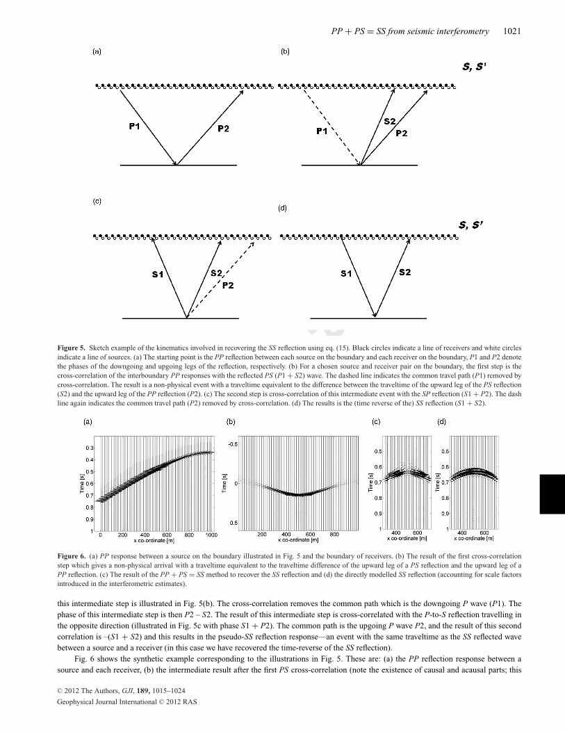
Figure 5. Sketch example of the kinematics involved in recovering the SS reflection using eq. (15). Black circles indicate a line of receivers and white circlesindicate a line of sources. (a) The starting point is the PP reflection between each source on the boundary and each receiver on the boundary, P1 and P2 denotethe phases of the downgoing and upgoing legs of the reflection, respectively. (b) For a chosen source and receiver pair on the boundary, the first step is thecross-correlation of the interboundary PP responses with the reflected PS (P1 + S2) wave. The dashed line indicates the common travel path (P1) removed bycross-correlation. The result is a non-physical event with a traveltime equivalent to the difference between the traveltime of the upward leg of the PS reflection(S2) and the upward leg of the PP reflection (P2). (c) The second step is cross-correlation of this intermediate event with the SP reflection (S1 + P2). The dashline again indicates the common travel path (P2) removed by cross-correlation. (d) The results is the (time reverse of the) SS reflection (S1 + S2).

Figure 6. (a) PP response between a source on the boundary illustrated in Fig. 5 and the boundary of receivers. (b) The result of the first cross-correlationstep which gives a non-physical arrival with a traveltime equivalent to the traveltime difference of the upward leg of a PS reflection and the upward leg of aPP reflection. (c) The result of the PP + PS = SS method to recover the SS reflection and (d) the directly modelled SS reflection (accounting for scale factorsintroduced in the interferometric estimates).

this intermediate step is illustrated in Fig. 5(b). The cross-correlation removes the common path which is the downgoing P wave (P1). Thephase of this intermediate step is then P2 – S2. The result of this intermediate step is cross-correlated with the P-to-S reflection travelling inthe opposite direction (illustrated in Fig. 5c with phase S1 + P2). The common path is the upgoing P wave P2, and the result of this secondcorrelation is –(S1 + S2) and this results in the pseudo-SS reflection response—an event with the same traveltime as the SS reflected wavebetween a source and a receiver (in this case we have recovered the time-reverse of the SS reflection).

Fig. 6 shows the synthetic example corresponding to the illustrations in Fig. 5. These are: (a) the PP reflection response between asource and each receiver, (b) the intermediate result after the first PS cross-correlation (note the existence of causal and acausal parts; this

C© 2012 The Authors, GJI, 189, 1015–1024



intermediate step is non-physical), (c) the pseudo-SS reflection response between a source and a line of receivers and (d) the directly modelledSS reflection response for comparison (right-hand panel). Note that as in Fig. 4(c), the traveltimes are correctly recovered using this method,but there are differences in amplitudes of the estimated response and directly computed response. In this case, these cannot be removed byapplying a single-scale factor, because they are caused by neglecting the (dynamically varying) terms with S-wave sources to reach eq. (14).

Thus, in this second configuration sketched in Fig. 5, the SS reflection response is constructed without the use of any S-wave sourcecomponents. This special case is different to the general case in which S sources are required to construct the SS responses, and it requiresthat both source and receiver boundaries are collocated, and that the particular source and receiver between which the Green’s function is tobe constructed also lie on the same source/receiver boundary.

Note that we have considered the result of two cross-correlations to recover the SS response. This is consistent with eq. (15) whichcontains two complex conjugations. However, Grechka & Dewangan (2003) show that the SS response can be recovered from the result of across-correlation and a convolution. If we take the complex conjugate of both sides of eq. (15), we find

Gr∗ψq ψm

(x2, x1) − Grψq ψm

(x2, x1) ≈ 4ω2

cP cP ′ρ2

∫S

∫S′

Grψq ψ0

(x2, x)Gr∗ψ ′

0ψ0(x′, x)Gr

ψmψ ′0(x1, x′) dS′ dS. (16)

There is only a single complex conjugate on the right-hand side of eq. (16). Thus, we now have an equation equivalent to the approachof Grechka & Dewangan (2003), containing one cross-correlation and one convolution. Let us use the phases defined earlier to illustratethat the correlation–convolution approach yields the time reverse (complex conjugation) of the correlation–correlation approach. Earlier, weconsider the correlation of the PP reflection response (P1 + P2), with the PS reflection response (P1 + S2): P1 + P2 − (P1 − S2) = P2 −S2. This intermediate step is then cross-correlated with the SP reflection response (S1 + P2): P2 – S2 – (S1 + P2) = – (S1 + S2). In thecorrelation–convolution case, the PS reflection response is convolved with the SP reflection response: P1 + S2 + S1 + P2. This intermediatestep is then cross-correlated with the PP reflection response: P1 + S2 + S1 + P2 − (P1 + P2) = S1 + S2. Therefore, we see that thecorrelation–convolution approach used by Grechka & Dewangan (2003) is equivalent to the complex conjugate of the correlation–correlationapproach that we have considered here.

D I S C U S S I O N

Using two different equations derived from the same starting point, we have shown that it is possible to recover the SS reflection response intwo different configurations. In the first case, the SS reflection response was recovered by cross-correlating direct S waves with reflected Swaves. In this normal configuration for source–receiver interferometry, the SS reflection response between a source and a receiver is recovered(with the correct amplitude-versus-offset behaviour) without having a direct recording of that reflection. In the second case, we showed thatthe SS reflection response can be recovered, even if we neglect all the terms requiring a shear wave source. In this second case, reflected Swaves are cross-correlated with reflected P waves. Thus, the SS response can be recovered using recordings of P and S waves due to P-wavesources only, as shown by Grechka & Tsvankin (2002). The synthetic example illustrates that while the kinematics of this response are correct,the dynamics are not. Using geometrical arguments illustrated in Fig. 5, we have shown that for this second approach to be successful allsources and receivers must be located on the same surface.

Thus, the key differences in eq. (15) from eq. (10) are:

(1) Source–receiver reciprocity is applied to one of the inputs, requiring that all sources and receivers must be located on the same surface;(2) The SS reflection response is recovered despite neglecting the S-wave sources required by theory;(3) All direct wave contributions are neglected;(4) All sources and receivers must be located on the same surface.

By neglecting the S-wave sources when applying eq. (15), we introduce amplitude errors in Fig. 6(c). For example, since there are noS-wave sources, the PS responses are used, and the PS response tends towards zero amplitude at zero offset (this was also noted by Grechka& Dewangan 2003).

Using the generalized relationship in eq. (8), we can also derive other relationships between P- and S-wave sources and receivers. Forexample, by following the same steps used to reach eq. (9), but with Q = 0, M = 0 (P-wave source, P-wave receiver), we can write

−4

ρ2

∫S

∫S′

∂ j G∗ψ0ψk


(x′, x)G∗ψ ′

kψ0(x′, x1)n j ′ n j dS′dS = Gψ0ψ0

(x2, x1) − G∗ψ0ψ0

(x2, x1)

+ 4

ρ2

∫S

∫S′

∂ j G∗ψ0ψ0

(x2, x)∂ j ′ Gψ ′0ψ0

(x′, x)G∗ψ ′

0ψ0(x′, x1)n j ′ n j dS′dS

+ 4

ρ2

∫S

∫S′

∂ j G∗ψ0ψk

(x2, x)∂ j ′ Gψ ′0ψk

(x′, x)G∗ψ ′

0ψ0(x′, x1)n j ′ n j dS′dS

+ 4

ρ2

∫S

∫S′

∂ j G∗ψ0ψ0

(x2, x)∂ j ′ Gψ ′kψ0

(x′, x)G∗ψ ′

kψ0(x′, x1)n j ′ n j dS′dS.

(17)

As in eq. (9), all terms dependent on the SS response have been moved to the left-hand side. Note, with Q = 0 and M = 0, only oneterm in the entire equation is dependent on the SS response, and it lies within a surface integral. Eq. (17) could, therefore, be used to

C© 2012 The Authors, GJI, 189, 1015–1024



formulate an inverse problem to find Gψ ′

kψk(x′, x) given all combinations of PP and PS responses; such an approach is equivalent to applying

the multidimensional deconvolution approach to solving interferometric equations (e.g. Wapenaar et al. 2008, 2011; van der Neut et al.2011).

In the Introduction, we discussed various methods based on the standard single integral form of interferometry that use P and S waves(or estimates of those) as inputs, for example, the work of Gaiser & Vasconcelos (2010) on seabed data, Bakulin & Mateeva’s (2008) workon downhole data, Miyazawa et al.’s (2008) work on ambient noise in a downhole setting, the developments of van der Neut et al. (2011) inthe application of multidimensional deconvolution and the application of Tonegawa & Nishida (2010) to deep earthquake recordings. Thus,we envisage that the representations derived here will find similar applications, but rather than being used to derive new responses betweenpairs of receivers (or pairs of sources) the new representations explain how new types of wavefields can be derived between existing sourcesand existing receivers.

Potential applications of the new source–receiver responses are discussed in Curtis & Halliday (2010), for example, in determiningsource-to-receiver surface wave (or ground-roll noise) estimates, replacing bad or faulty channels in a seismic survey, or as a quality controlmeasure for the results of other forms of seismic interferometry. Furthermore, King & Curtis (2012) show that double-integral source–receiverrepresentations can be used to correct non-physical errors present in the Green’s functions estimates from single-integral forms of seismicinterferometry when applied, for example, to towed streamer, or other one-sided survey geometries. Poliannikov (2011) show that similarinterferometric relations can be used to recover underside reflections using surface sources and receivers, and the internal-multiple predictionmethod developed by Weglein and co-workers also uses a similar combination of correlations and convolutions (e.g. Weglein et al. 1997).With multicomponent recordings allowing the separation of P- and S-wave data, our methods extend existing forms of interferometry to beable to be used with separated P- and S-wavefields.

Also note that the representations derived here are closely related to imaging methods, and therefore allow extension of those imagingmethods to P- and S-wave separated wavefields. For example, Halliday & Curtis (2010) show that the imaging method of Oristaglio (1989)is a special case of the acoustic scattering form of source–receiver interferometry, and Vasconcelos et al. (2010) link source–receiverinterferometry to so-called extended images that are used for localized velocity analysis.

Note from Fig. 5(b) that the intermediate step is equivalent to the difference in traveltime between the upgoing P and upgoing S legs ofthe PP and PS reflection responses, respectively. This could be considered as equivalent to a seismological receiver function where transmittedP and S waves are deconvolved to give an event with a traveltime equivalent to that illustrated in Fig. 5(b) (Galetti & Curtis 2012). Therefore,application of the second step in the PP + PS = SS method could be considered to be equivalent to the correlation of a receiver functionwith a PS reflection response (or convolution where the complex conjugate form in eq. 16 is used). This observation could lead to a methodwhere an SS response is recovered from transmitted wavefields, or a combination of transmitted wavefields and surface seismic data. Ikelle& Gangi (2007) also discuss the construction of physical events via a non-physical intermediate step. They refer to this intermediate step asa virtual reflection, and show how it can be used to predict internal multiples.

C O N C LU S I O N S

We have derived generalized source–receiver interferometric integrals for P and S waves, and have shown how these integrals can be used tocalculate the SS reflection response between a source and a receiver using wavefields emitted by that source and recorded on other receivers,and wavefields emitted by other sources and recorded only on that receiver. Thus, this SS reflection response can be calculated without directlyrecording it.

We have shown that the PP + PS = SS method is a special case of these source–receiver integrals, and have identified the key differencesbetween this method and the fully generalized form. These key differences are that the S-wave sources are neglected, source–receiverreciprocity must be applied to one of the inputs of the PP + PS = SS method, and this in turn requires that sources and receivers must becolocated on the same surface. Since this results in singularities where zero offset Green’s functions exist, only the reflected (scattered) partof the wavefield is used.

The generalized form includes all components of any source and receiver type, and allows derivation of other new relationships betweenP- and S-wave source and receivers. For example, we have also shown that the new relationships may be used to formulate an inverse problemto estimate SS responses from PP and PS responses. The new relationships may aid in combining existing P- and S-wave interferometry andimaging methods and source–receiver interferometry and imaging methods to find new applications in acquisition and processing, and inimaging and inversion of P- and S-wave data.

Finally, we noted that the intermediate step of the PP + PS = SS method may be considered as being equivalent to a receiver function,which suggests there may be a possibility of applying a similar technique using transmitted wavefields.

A C K N OW L E D G M E N T S

We would like to thank Jeannot Trampert, Vladimir Grechka and an anonymous reviewer for their comments and suggestions which helpedto improve the manuscript.

C© 2012 The Authors, GJI, 189, 1015–1024



R E F E R E N C E S

Bakulin, A. & Mateeva, A., 2008. Estimating interval shear-wave split-ting from multicomponent virtual shear check shots, Geophysics, 73(5),A39–A43.

Curtis, A. & Halliday, D., 2010. Source-receiver interferometry from uni-fied representation theorems, Phys. Rev. E, 81(4), 046601-1–046601-10.

Curtis, A. & Robertsson, J.O.A., 2002. Volumetric wavefield recording andnear-receiver group velocity estimation for land seismic, Geophysics,67(5), 1602–1611.

Curtis, A., Nicolson, H., Halliday, D., Trampert, J. & Baptie, B., 2009. Virtualseismometers in the subsurface of the Earth from seismic interferometry,Nature Geosci., 2, 700–704, doi:10.1038/NGEO615.

Gaiser, J.E. & Vasconcelos, I., 2010. Elastic interferometry for ocean bottomcable data: theory and examples, Geophys. Prospect., 58(3), 347–360.

Galleti, E. & Curtis, A., 2012. Generalised receiver functions and seismicinterferometry, Tectonophysics, in press.

Grechka, V. & Dewangan, P., 2003. Generation and processing of pseudo-shear-wave data: theory and case study, Geophysics, 68(6), 1807–1816.

Grechka, V. & Tsvankin, I., 2002. PP + PP = SS, Geophysics, 67(6),1961–1971.

Halliday, D. & Curtis, A., 2010. An interferometric theory of source-receiverscattering and imaging, Geophysics, 75(6), SA95–SA103.

Hong, T.-K. & Menke, W., 2006. Tomographic investigation of the wearalong the San Jacinto fault, southern California, Phys. Earth planet.Inter., 155, 236–248.

Ikelle, L.T. & Gangi, A.F., 2007. Negative bending in seismic reflection asso-ciated with time-advanced and time-retarded fields, Geophys. Prospect.,55, 57–69.

King, S. & Curtis, A., 2012. Suppressing nonphysical reflections in Green’sfunction estimates using source-receiver interferometry, Geophysics, 77,Q15–Q25.

van Manen, D.-J., Curtis, A. & Robertsson, J.O.A., 2006. Interferometricmodeling of wave propagation in inhomogeneous elastic media usingtime reversal and reciprocity, Geophysics, 71(4), SI47–SI60.

Miyazawa, M., Snieder, R. & Venkataraman, A., 2008. Application of seis-mic interferometry to extract P and S wave propagation and observationof shear wave splitting from noise data at Cold Lake, Canada, Geophysics,73, D35–D40.

van der Neut, J., Thorbecke, J., Mehta, K., Slob, E. & Wapenaar, K., 2011.Controlled-source interferometric redatuming by cross-correlation and

multi-dimensional deconvolution in elastic media, Geophysics, 76(4),SA63–SA76.

Oristaglio, M.L., 1989. An inverse scattering formula that uses all the data,Inverse Probl., 5, 1097–1105.

Poliannikov, O.V., 2011. Retrieving reflections by source-receiver wavefieldinterferometry, Geophysics, 76(1), SA1–SA8.

Robertsson, J.O.A. & Curtis, A., 2002. Wavefield separation using denselydeployed, three component, single sensor groups in land surface seismicrecordings, Geophysics, 67(5), 1624–1633.

Robertsson, J.O.A., Blanch, J.O. & Symes, W.W., 1994. Viscoelastic finite-difference modeling, Geophysics, 59, 1444–1456.

Slob, E., Draganov, D. & Wapenaar, K., 2007. Interferometric electromag-netic Green’s functions representations using propagation invariants, Geo-phys. J. Int., 169, 60–80.

Snieder, R., Wapenaar, K. & Larner, K., 2006. Spurious multiples in seismicinterferometry of primaries, Geophysics, 71, SI111–SI124.

Tonegawa, T. & Nishida, K., 2010. Inter-source body wave propagationsderived from seismic interferometry, Geophys. J. Int., 183, 861–868,doi:10.1111/j.1365-246X.2010.04753.x.

Vasconcelos, I. & Snieder, R., 2008a. Interferometry by deconvolution, Part1—theory for acoustic waves and numerical examples, Geophysics, 73,S115–S128.

Vasconcelos, I. & Snieder, R., 2008b. Interferometry by deconvolution: Part2—Theory for elastic waves and application to drill-bit seismic imaging,Geophysics, 73, S129–S141.

Vasconcelos, I., Sava, P. & Douma, H., 2010. Nonlinear extended imagesvia image-domain interferometry, Geophysics, 75, 105–115.

Wapenaar, C.P.A. & Haime, G.C., 1990. Elastic extrapolation of seismicP- and S-waves, Geophys. Prospect., 38, 23–60.

Wapenaar, K., 2003. Synthesis of an inhomogeneous medium from its acous-tic transmission response, Geophysics, 68, 1756–1759.

Wapenaar, K. & Fokkema, J., 2006. Green’s function representations forseismic interferometry, Geophysics, 71(4), SI33–SI44.

Wapenaar, K., van der Neut, J. & Ruigrok, E., 2008. Passive seismicinterferometry by multidimensional deconvolution, Geophysics, 73,A51–A56.

Wapenaar, K., van der Neut, J., Ruigrok, E., Draganov, D., Hunziker, J.,Slob, E., Thorbecke, J. & Snieder, R., 2011. Seismic interferometry bycrosscorrelation and by multi-dimensional deconvolution: a systematiccomparison, Geophys. J. Int., 185, 1335–1364.

Weglein, A.B., Gasparotto, F.A., Carvalho, P.M. & Stolt, R.H., 1997. Aninverse-scattering series method for attenuating multiples in seismic re-flection data, Geophysics, 62, 1975–1989.

C© 2012 The Authors, GJI, 189, 1015–1024


geophysical journal international - geos.ed.ac.uk d. halliday, a. curtis and k. wapenaar to use...

Documents