geophysicae annales a one-way nested eddy resolving … one-way nested eddy resolving model of the...

Annales Geophysicae (2003) 21: 205–220c© European Geosciences Union 2003Annales

Geophysicae

A one-way nested eddy resolving model of the Aegean and Levantinebasins: implementation and climatological runs

G. Korres and A. Lascaratos

Department of Applied Physics, University of Athens, Athens, Greece

Received: 7 June 2001 – Revised: 7 November 2001 – Accepted: 21 January 2002

Abstract. The present study deals with the implemen-tation of an eddy resolving model of the Levantine andAegean basins and its one-way nesting with a coarse res-olution (1/8◦ × 1/8◦) global Mediterranean general circula-tion model. The modelling effort is done within the frame-work of the Mediterranean Forecasting System Pilot Projectas an initiative towards real-time forecasting within the east-ern Mediterranean region.

The performed climatological runs of the nested modelhave shown very promising results on the ability of the modelto capture correctly the complex dynamics of the area and atthe same time to demonstrate the skill and robustness of thenesting technique applied.

A second aim of this study is to prepare a comprehensiveclimatological surface boundary conditions data set for theMediterranean Sea. This data set has been developed withinthe framework of the same research project and is suitablefor use in ocean circulation models of the Mediterranean Seaor parts of it. The computation is based on the ECMWF 6-hatmospheric parameters for the period 1979–1993 and a cali-brated set of momentum and heat flux bulk formulae resultedfrom previous studies for the Mediterranean region.

Key words. Oceanography: general (numerical modelling);physical (general circulation; air-sea interactions)

1 Introduction

Within the framework of the Mediterranean ForecastingSystem Pilot Project (hereafter MFSPP), an eddy resolv-ing ocean model of the Aegean and Levantine basins(ALERMO) has been developed. ALERMO, with a hor-izontal resolution of 1/20◦ × 1/20◦, acts as an intermedi-ate between the global Mediterranean general circulationmodel (Roussenov et al., 1995; Pinardi et al., 1997; Pinardiand Masetti, 2000), hereafter OGCM, and the various east-ern Mediterranean high-resolution shelf models developed

Correspondence to:G. Korres ([email protected])

within the same project. Such a modelling effort is ratherchallenging for the oceanography of the eastern Mediter-ranean since it was the first time models with such a highresolution have been implemented within this region. On theother hand, the whole effort prepares the prerequisites forthe operational oceanography of the region, which will bethe near future phase of the project.

In this paper, we present the development of the ALERMOmodel, the nesting technique with the OGCM, along withthe results from the climatological runs of the model. Previ-ous modelling studies in this area address the problem of theLevantine Intermediate Water (LIW) formation process (Las-caratos and Nittis, 1998), using the Princeton primitive equa-tion model (POM) and the simulation and understanding ofthe internal dynamics of the area, using a quasi-geostrophicmodelling approach (Robinson and Golnaraghi, 1993; Gol-naraghi, 1993). Both modelling efforts and a subsequent oneby Lascaratos et al. (1999), attempting to simulate the recentchanges in the deep thermohaline circulation of the easternMediterranean, have been designed in a stand-alone modelcontext. In this study, for the first time we address the prob-lem of nesting a high resolution general circulation modelof the whole eastern Mediterranean with a coarse resolutionglobal Mediterranean general circulation model (OGCM).Nesting procedures, although quite old and well set withinthe weather forecast context, are still open research issuesin operational oceanography. Even for the scales of theMediterranean basin, computational constraints still makethe simulation of high resolution domains quite a significantchallenge. The rather simple nesting technique adopted inthis study allows for the high resolution model (ALERMO)to have simultaneous independent radiative boundary condi-tions and dependent nested boundary conditions provided bythe OGCM. Such a nesting technique guarantees free passageof unwanted wave energy through the boundary of the highresolution model and at the same time modifies the inner so-lution according to the coarse resolution model (OGCM) dy-namics. Although this nesting implementation is done hereon a climatological basis, ongoing work (to be presented

206 G. Korres and A. Lascaratos: A one-way nested eddy resolving model of the Aegean and Levantine basins

5 0 5 10 15 20 25 30 3530

32

34

36

38

40

42

44

46

(a) F ebruary

5 0 5 10 15 20 25 30 3530

32

34

36

38

40

42

44

46

(b) August

FIGURE 1

5 0 5 10 15 20 25 30 3530

32

34

36

38

40

42

44

46

(a) F ebruary

5 0 5 10 15 20 25 30 3530

32

34

36

38

40

42

44

46

(b) August

FIGURE 1

Fig. 1. (a)Wind stress field for Febru-ary (b) Wind stress field for August.

in a forthcoming paper) in a July/September 1999 hindcastsimulation experiment, using 6-h atmospheric forcing, hasdemonstrated its robustness.

The second aim of this study is the development of a“perpetual year” surface boundary conditions data set (windstresses, net solar and long-wave radiation, latent and sen-sible heat flux) for the whole Mediterranean, to be used bythe OGCM, as well as by all intermediate and shelf modelswithin the same project. The study of Castellari et al. (1998)has dealt with the similar problem of formulating a calibratedset of heat flux bulk formulae to be used by the Mediter-ranean basin general circulation models. In the same context,Garrett et al. (1993) examined and estimated the Mediter-ranean heat budget using the COADS (Slutz et al., 1985)1946–1988 data set. In the latter study, latent and sensibleheat fluxes are partially estimated from instantaneous values,while the turbulent exchange coefficients and the long-waveradiation are computed using monthly mean values. In thispaper, we apply Castellari et al. (1998) suggested “best set”of bulk formulae to the ECMWF high-frequency (6-h) atmo-spheric data set, covering a 15-year period (January 1979–December 1993), to derive new monthly heat and momentumflux estimates for the Mediterranean basin. As an alternative,we have substituted Kondo’s scheme (suggested by Castellariet al., 1998) for the computation of latent and sensible heatflux, with Budyko’s bulk formula (Budyko, 1963), originallyproposed to be used with monthly values of atmospheric pa-rameters. As explained in Sect. 2, this was done in order tocompensate for the known relatively low wind speed valuesof the 15-year ECMWF data set.

The paper has been organized as follows. In Sect. 2 wepresent the methodology followed for the preparation of thenew surface boundary conditions data set. Results are dis-cussed and intercompared with previous similar studies. Thenext section deals with the ALERMO model setup, the im-plementation of the nesting open boundary conditions andthe climatological runs of the model. A thorough descrip-tion of the eastern Mediterranean climatological circulationpicture, as revealed by the model results, is also given here.Finally, in Sect. 4 we offer a brief summary of the main re-sults.

2 Preparation of the climatological atmospheric forcing

In this section, we present the procedures followed in orderto prepare the climatological atmospheric forcing data set,which was used to force the OGCM, intermediate and shelfmodels within the project. This new atmospheric forcing dataset consists of heat flux fields and wind stress components ona monthly basis, derived from the ECMWF 1979–1993 6-hre-analysis atmospheric parameters on a regular 1◦

× 1◦ grid.Below we explain in detail the methodology we used for thederivation of each of the different heat flux components andthe wind stress fields.

2.1 Wind stress components

The calculation of the climatological wind stress fields isbased on the transformation of the 6-h ECMWF wind ve-locity data at 10 m, to the zonal/meridional components of

G. Korres and A. Lascaratos: A one-way nested eddy resolving model of the Aegean and Levantine basins 207

3 2.5 2 1.5 1 0.5 0 0.5 1 1.5 2 2.5

x 10� 7

� 5 0 5 10 15 20 25 30 3530

32

34

36

38

40

42

44

46

FIGURE 2

Fig. 2. Wind stress curl difference between February and August.Units are Nt/ m3.

the wind stress exerted on the sea surface, according to theformula:

τ = ρACD|W |W , (1)

whereρA is the air density,W is the wind velocity andCD

is the drag coefficient, which is calculated every 6 h as afunction of wind speed and air-sea temperature differencethrough a polynomial approximation given by Hellermanand Rosenstein (1983). SST data are taken from Reynolds1◦

× 1◦ monthly 1979–1993 data set (linearly interpolatedevery 6 h), while air temperature data at 2 m above sea sur-face are taken from the ECMWF 1979–1993 re-analysis data.Finally, the air density in Eq. (1) is calculated as a functionof air temperature and relative humidity.

The 6-h zonal and meridional components of the windstress time series, as computed by Eq. (1), are then aver-aged in time, in order to form monthly climatological fieldsfor the Mediterranean region. In Fig. 1 we show the windstress field for a typical winter and summer month. The mostpronounced features during wintertime are the strong Mistralwinds over the western Mediterranean, blowing from north-west, and the northeasterlies over the Aegean Sea chang-ing progressively to northwesterlies over the eastern Levan-tine basin. Quasi-zonal winds prevail over the Ionian Sea,while the Bora wind pattern is evident within the AdriaticSea. The summer regime is characterized by differences inthe wind stress curl pattern over large parts of the basin, asshown in Fig. 2, presenting the difference in the wind stresscurl between the peaks of the winter (February) and sum-mer (August) seasons. Differences are most pronounced overthe western Mediterranean and the Ionian Sea. However,within the Levantine basin and the Aegean Sea, the seasonalchanges are perceptibly weaker. It is worth mentioning herethat the monthly wind stress fields produced with this par-ticular method from the ECMWF re-analysis wind velocitydata, compare very well with the wind stress fields, as calcu-lated by Hellerman and Rosenstein (1983) for the Mediter-ranean region.

175 180 185 190 195 200 205 210 215 220 225

5 0 5 10 15 20 25 30 3530

32

34

36

38

40

42

44

46

FIGURE 3

Fig. 3. Mean annual distribution of net short-wave radiation at thesea surface (in W/m2).

2.2 Solar radiation

The calculation of the absorbed solar radiation at theMediterranean Sea surface is based on the Reed formula(Reed, 1977), as already done in Rosati and Miyakoda,(1988) for the global ocean, Garrett et al. (1993) and Castel-lari et al. (1998) for the Mediterranean region:

Qs = QTOT (1 − 0.62C + 0.0019β) (1 − α) , (2)

whereQtot is the total solar radiation reaching the ocean sur-face under a clear sky,β is the solar noon altitude andαis the sea surface albedo. The cloud coverC in Eq. (2) istaken from COADS 1◦ × 1◦ monthly data set for the period1979–1993 instead of ECMWF re-analysis data. An inter-comparison (not shown) between basin average ECMWF(as derived from 6-h data) and COADS observational cloudcover monthly climatologies shows a systematic underesti-mation of the cloud coverage (especially during the cold sea-son) by the ECMWF data set. This is in agreement withJakob (1999), who evaluated the cloud cover in the ECMWFre-analysis data for the period 1983–1990 and pointed out anunderestimation of extratropical cloud cover over the oceansby 10%–15%.

The linear dependence of the Reed formula on cloud coverpermits us, without significant error, to apply this formulausing monthly averages of cloud cover.

Monthly values of solar insolation at each grid point areestimated after appropriate averaging of hourly values, ascomputed according to Eq. (2).

In Fig. 3 we show the mean annual pattern of the net short-wave radiation over the Mediterranean basin. It is charac-terized by a north-south gradient, with maximum solar heat-ing occurring over the southeasternmost part of the Levantinebasin. The basin’s mean annual solar radiation absorbed bythe Mediterranean basin amounts to 202 W/m2, which is thesame value as Castellari et al. (1998) calculated.


2.3 Net long-wave radiation

Bignami et al. (1995) proposed a bulk formula for the cal-culation of net long-wave radiation at the sea surface, whichwas strictly derived from regression to long-wave radiationmeasurements within the western Mediterranean. Up to now,this has been the most appropriate formula for the calcula-tion of long-wave radiation within the Mediterranean Sea,although one could argue that this formula is more repre-sentative of the western Mediterranean oceanic and meteo-rological conditions. Actually, very recently, Schiano et al.(2000) have stressed the importance of adjusting the Bignamiformula to the different areas of the Mediterranean Sea oreven inventing a new bulk formulae by taking into accountthe complex climatic conditions prevailing over the Mediter-ranean region. However, such an adjustment is out of thescope of the present paper, since it requires an extensive dataset of direct net long-wave radiation measurements over thewhole Mediterranean basin.

Following Bignami et al. (1995), the net long-wave radia-tion at the sea surface is given by:

QB = εσT 4s −

[σT 4

A(0.653+ 0.00 535eA)]

·

(1 + 0.1762C2

), (3)

where ε, σ are the sea surface emissivity and the Stefan-Boltzman constant, respectively,C is the cloud cover,eA isthe atmospheric vapor pressure andTS, TA are the SST andair temperature at 2 m height above the sea surface, respec-tively. The atmospheric vapor pressure is proportional to therelative humidityr:

eA = reSAT(TA),

where eSAT is the atmospheric saturation vapor pressure,computed through a polynomial approximation as a functionof air temperature (Lowe, 1977).

The computation ofQB is done every 6 h, using the1979 –1993 ECMWF atmospheric parameters of air temper-ature and relative humidity, and SST data from Reynolds’(Reynolds, 1994) 1979–1993 monthly data set (1◦

× 1◦) afterit has been linearly interpolated in time. We should point outhere that a bulk formula with a linear dependence on cloudcover should be preferable to be used when monthly values ofcloud cover are available (COADS cloud cover data). How-ever, the Bignami formula, being the only one tuned withinthe Mediterranean region, is our unique choice for the esti-mation of the net long-wave radiation, although we expectsome possible error due to the type (monthly versus instan-taneous) of cloud cover data we used.

Monthly fields ofQB are obtained by appropriate averag-ing of the 6-h time series obtained by Eq. (3) at each gridpoint. On a yearly basis, Bignami’s formula presents an in-creased net long-wave heat loss over the northern parts of theMediterranean Sea and within the eastern Levantine basin.The basin’s average time series ofQB (not shown) is char-acterized by a maximum of 100 W/m2 during January and a

minimum value of 80 W/m2 during August, while the meanannual value of net long-wave radiation is 90.3 W/m2.

2.4 Latent and sensible heat flux

The latentQe and sensibleQh heat fluxes are computed ac-cording to the classical bulk aerodynamic formulae (Rosatiand Miyakoda, 1988; Castellari et al., 1998):

Qe = ρALV CE |W |

[eSAT(TS) − reSAT(TA)

]0.622

pA

(4)

Qh = ρAcpCH |W |(TS − TA) , (5)

whereρA is the density of moist air (computed as a func-tion of air temperature and relative humidity),cp is the spe-cific heat capacity of atmospheric air,pA is the atmosphericpressure andW represents the horizontal wind velocity vec-tor at 10 m above sea surface. The latent heat of vaporiza-tion, LV , is calculated as a function of sea surface temper-ature (Gill, 1982). CE andCH are the turbulent exchangecoefficients both taken equal to 2.1 × 10−3 in the “neutralBudyko scheme”, as proposed by (Budyko, 1963). Budykoimposed these large values for the turbulent exchange coeffi-cients, since he had to deal with monthly values of the atmo-spheric parameters that inevitably lead to an underestimationof the turbulent heat fluxes through the air-sea interface. Inthe scheme known as “Kondo scheme” (Kondo, 1975), theturbulence exchange coefficients in diabatic conditions (sta-ble or unstable) are estimated in terms of the sea-air tempera-ture difference and the wind speed, along with an index of at-mospheric stability that nonlinearly modulates them. Castel-lari et al. (1998), using twice daily NCEP 1980–1988 atmo-spheric data (1◦ × 1◦), COADS monthly cloud cover data(1◦

×1◦) for the same period and Reynolds (Reynolds, 1994)1980–1988 monthly SST (1◦

× 1◦), have selected the Kondoscheme as the most appropriate for the computation of latentand sensible heat flux. In particular, taking into considera-tion the terrestrial branch of the water cycle of the Mediter-ranean, they estimate the Mediterranean evaporation rate torange between 1.32–1.57 m/yr, which corresponds to a rangeof Qe between 103–122 W/m2. The annual mean basin av-erage value ofQe that they have obtained with the Kondoscheme is 122 W/m2, while the neutral Budyko scheme re-sulted in a much higher value in their case (170 W/m2) thathad to be rejected on the grounds of the acceptable evapora-tion range.

In our case, we have estimated the latent and sensibleheat flux using both schemes (i.e. the Kondo and the neu-tral Budyko scheme) and intercompare the results in termsof the acceptable evaporation range suggested by Castellariet al. (1998). For both schemes we form 6-h values ofQe andQh using the ECMWF 1979–1993 re-analysis data (1◦

× 1◦)for the atmospheric parameters of air temperature, relativehumidity and wind speed, while the cloud cover data aretaken from the COADS 1979–1993 monthly cloud cover data(1◦

×1◦) and the SST from the Reynolds 1979–1993 monthlydata set (1◦ ×1◦) . Finally, from the 6-h values ofQe andQh

we form a monthly mean data set with appropriate averaging.


60 70 80 90 100 110 120 130 140

5 0 5 10 15 20 25 30 3530

32

34

36

38

40

42

44

46(a)

60 70 80 90 100 110 120 130 140

5 0 5 10 15 20 25 30 3530

32

34

36

38

40

42

44

46(b)

FIGURE 4

60 70 80 90 100 110 120 130 140

5 0 5 10 15 20 25 30 3530

32

34

36

38

40

42

44

46(a)

60 70 80 90 100 110 120 130 140

5 0 5 10 15 20 25 30 3530

32

34

36

38

40

42

44

46(b)

FIGURE 4Fig. 4. Mean annual distribution of evaporative heat flux at thesea surface corresponding(a) to Kondo scheme and(b) to neutralBudyko scheme. Units are W/m2.

Budyko’s neutral scheme corresponds to a mean annualvalue of 106.2 W/m2, which is within the acceptable range ofvalues for the Mediterranean basin, while the Kondo schemecorresponds to a much lower value (82.9 W/m2). The meanannual spatial patterns corresponding to the two schemes areshown in Fig. 4. The increased value of the turbulent ex-change coefficient that the neutral Budyko scheme assumescompensates for the underestimated magnitude of the 10 mECMWF winds and thus, produces a correct basin meanvalue for the latent heat flux. However, by inspecting Fig. 4b,it is evident that this scheme overestimates the evaporationrate over the eastern Levantine basin. On the other hand, theKondo scheme leads to an underestimation of the evaporationrates over large parts of the Mediterranean basin.

2.5 Net heat flux

The net heat flux into the Mediterranean Sea consists of thesolar insolation minus the net long-wave radiation and thelatent and sensible heat fluxes:

Qt = Qs − QB − Qe − Qh . (6)

The results of the different heat flux bulk formulae are sum-marized in Table 1 in terms of annual mean values. TheBignami formula for the computation of net long-wave ra-diation, combined with the Kondo scheme for the calcula-tion of the latent and sensible heat flux, gives a positive

50 40 30 20 10 0 10 20 30 40 50

5 0 5 10 15 20 25 30 3530

32

34

36

38

40

42

44

46(a)

50 40 30 20 10 0 10 20 30 40 50

5 0 5 10 15 20 25 30 3530

32

34

36

38

40

42

44

46(b)

FIGURE 5

50 40 30 20 10 0 10 20 30 40 50

5 0 5 10 15 20 25 30 3530

32

34

36

38

40

42

44

46(a)

50 40 30 20 10 0 10 20 30 40 50

5 0 5 10 15 20 25 30 3530

32

34

36

38

40

42

44

46(b)

FIGURE 5Fig. 5. Mean annual distribution of total heat flux at the sea surfacecorresponding(a) to Kondo-Bignami and(b) to Budyko-Kondodata set. Units are W/m2.

(+17.9 W/m2) heat budget for the Mediterranean. We willrefer to this combination as the “Kondo-Bignami” data set.The spatial distribution of the mean annual net heat fluxcorresponding to the Kondo-Bignami data set is shown inFig. 5a. The optimum combination of bulk formulae in termsof the widely accepted basin average annual heat budget forthe Mediterranean basin (−7 W/m2) consists of the neutralBudyko scheme for the computation of latent and sensibleheat fluxes, along with the Bignami formula for the calcula-tion of the net long-wave radiation (we call this the “Budyko–Bignami” data set). According to Table I, this particular com-bination amounts to an annual heat budget of−7.2 W/m2. InFig. 5b we show the spatial distribution of the net heat fluxcorresponding to the Budyko-Bignami data set. The patternshown in this figure corresponds to a net heat loss over theLevantine and Aegean basins, the Adriatic Sea and the north-western sector of the western Mediterranean basin. The Io-nian basin presents an area of net heat gain, especially inits southwestern part. Comparison of Figs. 5a and b showsthat the two data sets involve almost the same spatial struc-ture apart from a positive offset of around 25 W/m2 of the“Kondo-Bignami” data set. In a Mediterranean modellingperspective, such a positive offset can be corrected by theappropriate choice of a heat flux correction term, as will beshown in what follows. Finally, it is interesting to point outthat both data sets (Budyko-Bignami and Kondo-Bignami)


Table 1. Heat budget components estimated with different formu-lations

Formulae Qs (W/m2) QB (W/m2) Qe (W/m2) Qh (W/m2)

Reed 201.67

Bignami 90.33

Neutral Budyko 106.18 12.42

Kondo 82.81 11.16

have spatial scales comparable with the ones existing in theGarrett and Outerbridge (1993) results (based on COADSdata), although these authors arrived at the correct globalMediterranean heat budget by reducing the short-wave ra-diation by 18%.

3 The numerical model

3.1 Model description

The ALERMO model is based on the Princeton Ocean Model(POM), a primitive equation, 3-D circulation model. POMhas been extensively described in the literature (Blumbergand Mellor, 1983, 1987; Oey et al., 1985a, b; Galperin andMellor, 1990a, b; Mellor and Ezer, 1991, Horton et al., 1997;Lascaratos and Nittis, 1998) and is accompanied by a com-prehensive user’s guide (Mellor, 1998). It has been usedpreviously in numerous coastal applications like the SouthAtlantic Bight (Blumberg and Mellor, 1983), Delaware Bay(Galperin and Mellor, 1990a, b), the Gulf of Mexico (Mel-lor and Blumberg, 1985), the Gulf Stream (Ezer and Mellor,1992), the Mediterranean Sea (Zavatarelli and Mellor, 1995;Horton et al., 1997; Drakopoulos and Lascaratos, 1997), theAdriatic Sea (Zavatarelli and Pinardi, 1995) and the Levan-tine Sea (Lascaratos and Nittis, 1998), to list some of them.

The model has a bottom-following vertical sigma coordi-nate system, a free surface and a split mode time step. Poten-tial temperature, salinity, velocity and surface elevation areprognostic variables. It solves the following equations forthe ocean velocityUi = (U, V,W), potential temperatureTand salinityS:

∂Ui

∂xi

= 0 (7)

∂

∂t(U, V ) +

∂

∂xi

[Ui(U, V )] + f (−V, U) =

−1

ρ0

[∂p

∂x,∂p

∂y

]+

∂

∂z

[KM

∂

∂z(U, V )

]+ (FU , FV ) (8)

∂T

∂t+

∂

∂xi

[UiT ] =∂

∂z

[KH

∂T

∂z

]+ FT (9)

∂S

∂t+

∂

∂xi

[UiS] =∂

∂z

[KH

∂S

∂z

]+ FS . (10)

The hydrostatic approximation yields:

p

ρ0= g(n − z) +

n∫z

ρ − ρ0

ρ0gdz , (11)

wheren is the free surface elevation,ρ0 is a reference densityandρ = ρ(T , S, p) is the density calculated by an adaptationof the UNESCO equation of state by Mellor (1991b). Thehorizontal diffusion termsFU , FV , FT andFS in Eqs. (8), (9)and (10) are evaluated using the Smagorinsky (1963) hori-zontal diffusion formulation.

The vertical mixing coefficientsKM andKH in Eqs. (8)-(10) are computed according to the Mellor-Yamada 2.5 tur-bulence closure scheme (Mellor and Yamada, 1982).

The ALERMO model has one open boundary located at20◦ E, as shown in Fig. 6. The computational grid has a hor-izontal resolution of 1/20◦

× 1/20◦ and 30 sigma layers inthe vertical, with a logarithmic distribution near the sea sur-face, which results in a better representation of the surfacemixed layer. Considering the size (10–14 km) of the inter-nal Rossby radius of deformation for the eastern Mediter-ranean basin (Robinson et al., 1987), such a model resolution(∼ 5 km) can marginally resolve the mesoscale eddy activity.Since this version of the ALERMO model is computationallyexpensive, a coarse version (1/10◦

× 1/10, 30 sigma layers)was also developed, in order to perform several sensitivitytests. For both versions of the model, the U.S. Navy DigitalBathymetric Data Base 5 (1/12◦

×1/12◦) was used for build-ing up the model’s bathymetry, using bilinear interpolation tomap the data onto the model’s grid.

3.2 Nesting technique

Nesting is a finite-difference technique to simulate a high-resolution domain embedded in a coarse resolution model.In our case the coarse resolution model is the global Mediter-ranean OGCM, which is one-way nested with the ALERMOmodel (fine grid model). By one-way nesting, we mean thatthe boundary conditions of the fine grid model are prescribedin some way by external data taken from the coarse resolu-tion model, while the solution of the latter is not modified bythe solution of the fine grid model in their common overlap-ping area. Of major importance in nesting techniques is theconservation of properties between the coarse and fine gridmodel, and the treatment of fine grid interior noise result-ing from several types of incompatibilities between the twomodels. The OGCM is the Modular Ocean Model (rigid-lidmodel) implemented within the Mediterranean region with a1/8◦

×1/8◦ horizontal resolution and 31 levels in the vertical.It was integrated for an 8-year period, using the climatologi-cal momentum and heat flux fields developed for the MFSPPproject (and presented in Sect. 2 of this paper), plus someadditional heat and freshwater correction terms. During thelast year of OGCM integration, model prognostic variablesare stored in the form of 10-day averages for further use bythe ALERMO and three other fine grid models (namely the


20 22 24 26 28 30 32 34 3630

32

34

36

38

40

400

400 4

00

800 800

800

800

800

800 800

800

1200

1200

1200

1200

1200

1200

1200

1200

1600

1600

1600

16

00

1600

1600

1600

1600

2000

2000

2000

2000

20

00

2000

2000

2000

2400

2400

2400

2400

2400

2400

2400

2400

2400

2800

2800

28

00

2800 2800

2800

2800

32003600

FIGURE 6

Fig. 6. ALERMO model topography in meters (contour interval: 200 m).

western Mediterranean, the Adriatic and the Sicilian straitsmodels) within the Mediterranean region.

The nesting with the global Mediterranean OGCM is ap-plied along the western boundary of ALERMO (located at20◦ E). The phenomenology of the area (Robinson et al.,1991) and previous modelling work (Lascaratos and Nittis,1998) suggest that this is a very important boundary for thewater mass exchange (inflowing waters of Atlantic origin andoutflowing LIW waters) of the Levantine basin and thus, toa large extent controls both the general and the thermohalinecirculation of the area.

The nesting between the two models involves the variablesUC , VC (zonal and meridional velocity components),TC , SC

(temperature and salinity) andnC (the sea surface height ascomputed from the surface pressure of the rigid lid model;Pinardi et al., 1995) of the coarse grid model (OGCM) andthe prognostic variablesUF , V F (the external mode zonaland meridional velocity components),UF , VF (the inter-nal mode zonal and meridional velocity components),TF ,SF , andnF (free surface elevation) of the fine grid model(ALERMO). During the ALERMO model run, the OGCM10-day averaged variablesUC , VC , TC , SC , andnC , are in-terpolated onto they−z open boundary section of ALERMOat each time step. The interpolated variables are denoted hereasU INT

C , V INTC , T INT

C , SINTC , andnINT

C , respectively. Inter-

polation in time is linear. The spatial interpolation is bilinearfor all OGCM model variables, with the additional constraintof volume conservation through the open boundary. The vol-ume conservation constraint is due to the fact that this partic-ular open boundary section (and any other section that startsand ends to the mainland) in the OGCM is constrained tosustain a zero net volume transport due to the rigid lid modelphysics. As a result, the interpolated fieldU INT

C is correctedin such a way that it guarantees volume conservation betweenthe coarse and the fine grid model:

y2∫y1

∫ 0

−H

U INTC dzdy = 0 , (12)

wherey1, y2 are the extremes of the open boundary section,while H is the ALERMO bathymetry at the open boundary.

3.2.1 OBCs for the external mode

The condition we use for the normal barotropic velocity (ex-ternal mode) at the open boundary of ALERMO is a modifiedFlather (1976) condition that efficiently allows for interiordisturbances – due to possible mismatches between coarseand nested values – to pass out through the lateral boundary.The Flather boundary condition initially proposed for tidal


0 60 120 180 240 300 3600.01

0

0.01

0.02

0.03

106 m

3 /s

Days

FIGURE 7

Fig. 7. Net volume transport time series at ALERMO’s open bound-ary (continuous line) and volume discharge into the Aegean Sea dueto the Dardanelles and river runoff (dashed line). Positive values ofvolume transport denote ouflow from the model domain. Units are106 m3/s.

models combines a Sommerfeld-type radiation condition:

∂n

∂t−

√gH

∂n

∂x= 0

with a one-dimensional version of the continuity equation:

∂[(H + n)U

]∂x

+∂n

∂t= 0

to yield a boundary condition for the normal barotropic ve-locity UF of ALERMO:

UF =H

H + nF

UINT

F +

√gH

H + nF

(nINT

c − nF

), (13)

where

UINT

F =1

H

0∫−H

U INTC dz.

A Sommerfeld boundary condition does not, in general, re-spect volume conservation. Due to this fact, one is forcedto apply volume conservation constraints (as done in March-esiello et al., 2001) in cases of significant imbalances be-tween the net volume transport at the open boundary and thetime variation of the total volume of the modelling domain.

In our case, as shown in Fig. 7, the net volume transportat the open boundary of ALERMO closely balances on theyearly basis the net inflow to the Aegean Sea due to Dard-anelles (mainly) and river runoff. As a result, the mean sealevel (not shown) does not show any systematic drift. Thus,no additional constraint is applied to the barotropic flow atthe open boundary.

The tangential barotropic velocity at the open boundary isdirectly prescribed from the OGCM:

V F = VINT

C . (14)

3.2.2 OBCs for the internal mode

The internal mode velocitiesUF andVF (normal and tan-gential) at the open boundary of ALERMO are directly pre-scribed from the OGCM:

UF =H

H + nF

U INTC VF = V INT

C , (15)

where the factorH/(H + nF ) guarantees volume continuity.

3.2.3 OBCs for temperature and salinity

To update the temperature and salinity profilesTF andSF atthe open boundary of ALERMO, we use an upstream advec-tion scheme whenever the normal velocity is directed out-wards from the modelling area:

∂TF

∂t+ UF

∂TF

∂x= 0

∂SF

∂t+ UF

∂SF

∂x= 0 UF < 0 . (16)

In cases of inflow through the open boundary, temperatureand salinity are prescribed directly from the interpolatedOGCM temperature and salinity profiles (T INT

C , SINTC ):

TF = T INTC SF = SINT

C UF > 0 . (17)

3.2.4 OBC for the free surface elevation

For the specification of the free surface elevation at the openboundary of ALERMO, we have adopted a zero-gradientcondition:

∂nF

∂x= 0 . (18)

3.3 Initial data

The ALERMO model is initialized directly from the OGCMmodel results obtained during the eighth year of its per-petual integration. Temperature, salinity, velocity (inter-nal/external) and sea surface height fields are all specifiedduring the initialization process from the OGCM. In orderto reduce the initial shock of the model as much as possi-ble, we decided to initialize ALERMO from summer aver-age conditions (15 August). The OGCM model results weremapped onto ALERMO’s grid, using bilinear interpolationin the horizontal and linear in vertical. Extrapolation tookplace only in limited areas along the northeastern coasts ofGreece, within the Cyclades region and adjacent to the AsiaMinor coasts, due to the coarse representation of these areasin the OGCM. The adjustment phase of the ALERMO modellasts for approximately 10–15 days and involves mainly thebarotropic circulation along the coastal areas of Asia Minorand northern Greece. Such a behaviour can be attributed tothe extrapolation of the OGCM values in these areas, whichthen triggers spurious flow divergences. By day 20 the flowfield is already smooth, as can be seen in the free surface ele-vation field presented in Fig. 8b. In Fig. 8a we show for com-parison the sea surface elevation as deduced from the OGCMcorresponding to 5 September. It is evident that in order to


20

15

10

5

0

5

10

15

20

20 22 24 26 28 30 32 34 3630

32

34

36

38

40

(a)

6

4

2

0

2

4

6

20 22 24 26 28 30 32 34 3630

32

34

36

38

40

(b)

FIGURE 8

20

15

10

5

0

5

10

15

20

20 22 24 26 28 30 32 34 3630

32

34

36

38

40

(a)

6

4

2

0

2

4

6

20 22 24 26 28 30 32 34 3630

32

34

36

38

40

(b)

FIGURE 8Fig. 8. (a)OGCM sea surface elevation field (5 September) as mapped onto ALERMO’s domain(b) ALERMO free surface elevation after20 days of climatological integration (units are cm).

decrease the duration of the adjustment phase of the modelas much as possible, more sophisticated techniques shouldbe used in order to extrapolate, when necessary, the coarsemodel data onto the fine grid.

3.4 Surface boundary conditions

3.4.1 Momentum boundary condition

The momentum boundary condition at the surface takes theform:

ρ0KM

∂uh

∂z

∣∣∣∣z=0

= τ , (19)

whereτ is the wind stress provided by ECMWF’s perpetualyear monthly climatology, as described in Sect. 2.

3.4.2 Heat flux boundary condition

For the heat flux boundary condition at the surface we as-sume:

ρ0cpKH

∂T

∂z

∣∣∣∣z=0

= QT + ca(T∗

− T ) , (20)

whereQT is the surface total heat flux field diagnosed fromthe eighth year of the OGCM climatological run. The termca(T

∗−T ) appearing in Eq. (20) acts as a further adjustment

of the diagnosed OGCM surface heat flux to the ALERMO’smodelling domain. Such an adjustment is justified consider-ing the possible climatic drift of the OGCM and the extrap-olation taking place in coastal areas (especially within thenorth Aegean Sea) when the OGCM fields are mapped ontoALERMO’s domain. TheT ∗ fields are taken from MODB-MED4 SST seasonal climatology (Brasseur et al., 1996),while ca is set to 5 Wm−2C−1.

The OGCM total heat flux field is originally provided as10-day averages and it is then linearly interpolated in timeat each time step of the ALERMO model integration. TheOGCM perpetual integration experiment has been forced

with the Kondo-Bignami heat flux data set, plus an addi-tional heat flux correction termc0(T

∗− TOGCM), where

c0 = 25 Wm−2C−1. The Kondo-Bignami data set, as al-ready mentioned in Sect. 2, corresponds to a strongly posi-tive (+17.3 Wm−2) annual heat budget for the Mediterraneanregion. This data set is then adjusted in the course of theOGCM climatological integration to yield net heat flux fields- as diagnosed during the eighth year of the OGCM simula-tion - corresponding to a global Mediterranean annual heatbudget equal to−4.9 Wm−2.

3.4.3 Salinity boundary condition

The salinity boundary condition at the surface is as follows:

KH

∂S

∂z

∣∣∣∣z=0

= S (E − P) + c2(S∗

− S)

(21)

whereS is the model’s sea surface salinity. The evaporationrateE was calculated from the latent heat fluxQe , as pro-vided by the Kondo-Bignami climatological data set:

E =Qe

ρLV

. (22)

In the above expressionLV is taken to be equal to 2.5008×

106 J/kg, andρ = 1023 kgm−3 is the density of seawater.The precipitation rateP is obtained from the Jaeger (1976)monthly precipitation climatology, initially mapped on a 5◦

×

2.5◦ grid. The correction termc2(S∗

− S) accounts for theimperfect knowledge ofE−P (especially of the precipitationrates). In this termS∗ is the seasonal MODB-MED4 seasurface salinity, andc2 has been set (upon sensitivity studies)equal to 0.7 m/day.

3.5 Parameterization of the Dardanelles outflowand river runoff

The Dardanelles outflow into the Aegean Sea is a dominantfactor for the freshwater budget of the basin, providing ap-proximately 300 km3 of brackish water on an annual basis.


0.5 1 1.5 2 2.5 3

2

3

4

5

6x 10

3K

.E. (

m2 /s

2 )

Years

a

0.5 1 1.5 2 2.5 3

13.95

14

14.05

14.1

Tem

pera

ture

(o C)

Years

b

0.5 1 1.5 2 2.5 338.747

38.748

38.749

38.75

38.751

38.752

38.753

38.754

Sali

nity

(ps

u)

Years

c

FIGURE 9

Fig. 9. Basin averaged time series of(a) kinetic energy(b) temperature and(c) salinity, corresponding to ALERMO’s climatologicalintegration.

0.5 1 1.5 2 2.5 3

0.2

0.4

0.6

0.8

1

1.2

1.4

1.6

Surf

ace

fres

hwat

er fl

ux (

m/y

r)

Years

a

0.5 1 1.5 2 2.5 3150

100

50

0

50

100

Surf

ace

heat

flux

(W

/m2 )

Years

b

FIGURE 10

Fig. 10. Basin averaged time series of(a) diagnosed surface freshwater flux and(b) diagnosed surface total heat flux, corresponding toALERMO’s climatological integration.


20 22 24 26 28 30 32 34 36

31

32

33

34

35

36

37

38

39

40

41

(a)

20 22 24 26 28 30 32 34 36

31

32

33

34

35

36

37

38

39

40

41

(b)

FIGURE 11

20 22 24 26 28 30 32 34 36

31

32

33

34

35

36

37

38

39

40

41

(a)

20 22 24 26 28 30 32 34 36

31

32

33

34

35

36

37

38

39

40

41

(b)

FIGURE 11

20 22 24 26 28 30 32 34 36

31

32

33

34

35

36

37

38

39

40

41

(c)

20 22 24 26 28 30 32 34 36

31

32

33

34

35

36

37

38

39

40

41

(d)

FIGURE 11 cont.

20 22 24 26 28 30 32 34 36

31

32

33

34

35

36

37

38

39

40

41

(c)

20 22 24 26 28 30 32 34 36

31

32

33

34

35

36

37

38

39

40

41

(d)

FIGURE 11 cont.Fig. 11. (a)ALERMO’s subsurface velocity field (30 m) during February,(b) as in Fig. 11a but for August(c) as in Fig. 11a but for theOGCM model(d) as in Fig. 11b but for the OGCM model.

The main Greek rivers (Axios, Aliakmonas, Gallikos, Pinios,Sperchios, Evros, Strimonas and Nestos), on the other hand,with a total runoff of∼ 19 km3/yr, have a lesser contributionto the freshwater budget. Even lower is the contribution ofthe Turkish rivers, with a total runoff of∼ 5 km3/yr (Pouloset al., 1997).

ALERMO includes parameterization of Dardanelles’ netoutflow into the Aegean Sea and the runoff of the major riversof the Thermaikos Gulf (Aliakmonas, Axios and Loudias).The net annual Dardanelles outflow to the Aegean Sea isconsidered to be 104 m3/s, with a seasonal modulation of5× 103 m3/s. Maximum values are reached during mid-July,while the minimum is in mid-January. The salinity of thiswater outflow is set equal to 28.3 psu throughout the year.The Thermaikos Gulf rivers’ runoff is specified according todaily climatological values, as provided by the Greek Min-istry of Agriculture. It ranges from between 28 and 324 m3/s,with a minimum at the end of July and a maximum in Febru-ary.

The water dischargeQj (wherej denotes the grid pointwhere the discharge is introduced andQj has units L3/T)for the Dardanelles outflow or the rivers’ runoff parameter-izations, is treated as a point source in the two-dimensional

continuity equation, which becomes:

∂n

∂t+

∂Du

∂x+

∂Dv

∂y=

Qj

Aj

,

whereD = H + n andAj = 1xj1yj .

Finally, the water surplus due to the rivers’ runoff andthe Dardanelles net outflow has the same temperature of themodel’s top layer at the specified grid point, whereas itssalinity, as already mentioned, is 28.3 psu for Dardanellesand 0.0 psu for the Gulf of the Thermaikos rivers.

This parameterization has been successfully used byKourafalou et al. (1996) for the study of rivers’ dischargeon continental shelves. We are aware that such a parameteri-zation for the Dardanelles inflow/outflow tends to underesti-mate the freshwater input into the north Aegean Sea, as com-pared with a lateral flux boundary condition (open boundarycondition). However, due to the inadequate knowledge ofinflow and outflow velocities at the Bosporus straits on a cli-matological basis, we preferred specifying the net water dis-charge (which is more accurately known) rather than usingan open boundary condition.


FIGURE 12

Fig. 12. Schematic upper thermocline general circulation (redrawnfrom Robinson et al., 1991).

3.6 Model results

Starting from the late summer initial conditions (15 Au-gust), the model was integrated for two and one-half suc-cessive years with open boundary conditions, initial data,forcing input and Dardanelles/river-runoff parameterizationsas described in Sects. 3.2, 3.3, 3.4 and 3.5, respectively.The basin’s averaged kinetic energy of the model (shown inFig. 9a) is quasi-stabilized after the second year of the perpet-ual integration. The same holds for the basin’s averaged tem-perature and salinity of the area (shown in Figs. 9b and 9c),although the basin’s averaged salinity time series is showinga decreasing trend. The time series of the diagnosed fresh-water flux (E−P+correction) and total heat flux (QT + cor-rection) at the surface (shown in Figs. 10a and 10b) are char-acterized by an average value of 0.72 m/yr and−10.4 W/m2

during the last year of integration, respectively.

3.6.1 Circulation patterns

In Figs. 11a and 11b we present the subsurface (30 m) win-ter (mid-February) and summer (mid-August) circulationpatterns corresponding to the second year of the climato-logical integration of the model. The circulation patternssuggest that the model can successfully reproduce all themain general circulation characteristics of the area (MidMediterranean Jet, Asia Minor Current, Rhodes cyclonicgyre, Mersa-Matruh and Shikmona anticyclonic gyres), re-vealed by the synthesis of the POEM data set (see Fig. 12adapted from Robinson et al., 1991). Both winter and sum-mer circulation patterns are very rich in mesoscale features,which are mainly intensified during the summer period. InFigs. 11c and 11d we show for intercomparison the circula-tion patterns corresponding to the eighth year of the OGCMclimatological run. It is evident from such an intercompar-ison that ALERMO is able to reproduce the general circu-lation picture as provided by the OGCM and enrich it withvarious mesoscale structures, especially in the easternmostLevantine basin.

Important seasonal variability characterizes the eastern-most Levantine basin and the southern central Levantine.In the former, we see the recurrence of the Shikmona an-ticyclone between winter and summer, while in the latterthe Mersa-Matruh gyre exhibits large variations in strength,shape and position. The Mid Mediterranean Jet (MMJ) iswell formed and shows significant seasonal variations in itspathways.

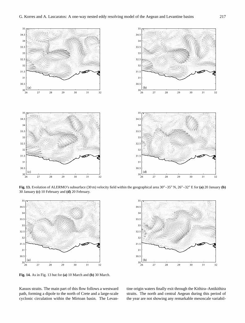
During winter, MMJ flows along the northern border of theMersa-Matruh gyre. Along its eastward path, several mean-derings take place, resulting in some cases in anticycloniceddy detachments to the north of the jet. Such a detach-ment process of an anticyclonic eddy is shown in Fig. 13 forfour successive snapshots taken every ten days, starting from20 January. The main part of MMJ departs from the Africancoast at approximately 25◦ E. Moreover, a cyclonic eddylocated near the African coast at 29◦ E completely blocksthe coastal branch of MMJ, which, in turn, feeds the MMJbranch along the northern border of Mersa-Matruh. As a re-sult, the northern branch reinforces and starts meandering tothe north at 30◦ E (Fig. 13a). Gradually, the meandering be-comes very steep (Figs. 13b and c) and finally leads to the de-tachment of an anticyclonic eddy, which then slowly movesto the north. The signal of this eddy is clearly evident at 300–400 m, while below this depth it is absent. At the beginningof March (Fig. 14a) the anticyclone moves very close to theMMJ and 20 days latter (Fig. 14b) it has been completelyrecaptured. Wintertime meandering of the MMJ within theeastern Levantine basin is not very pronounced. After its en-trance, it moves directly towards the Israeli coasts, where itturns to the west and encircles the Shikmona anticyclone.It subsequently moves to the northeast, enters the Lattakiabasin and finally feeds the Asia Minor current (AMC).

During summer the MMJ remains hugged to the Africancoast up to 29◦ E, and the Mersa-Matruh gyre, appearingnow as a three-lobe structure (Ozsoy et al., 1993; Malanotte-Rizzoli et al., 1999), is completely to the north of the jet.During this period of the year, Mersa-Matruh expands spa-tially and strengthens. As a result, the Rhodes gyre issqueezed to the north. The MMJ is not showing any mean-dering until it reaches the easternmost Levantine continentalshelf, where at approximately north of the Israeli coasts, itbifurcates into two branches. One branch flows to the north-west and the other continues to the north along the easternLevantine continental shelf. The northwestern branch, alongits path, forms a series of two cyclones and finally an anticy-clone to the southwest of Cyprus and then turns to the east toflow towards the eastern Levantine continental shelf follow-ing the 1000 m isobath to the south of Cyprus. This eastwardcurrent merges with the north branch flowing along the east-ern Levantine continental shelf at 34◦ N, and they both formtwo extended anticyclones east of Cyprus within the Lattakiabasin to finally feed the AMC.

In Fig. 15 we show a close-up of the Aegean circula-tion during the winter and summer periods. During the coldseason the AMC enters the Aegean Sea mainly through theRhodes–Karpathos straits and secondarily through the Crete-


26 27 28 29 30 31 3230

30.5

31

31.5

32

32.5

33

33.5

34

34.5

35

(a)

26 27 28 29 30 31 3230

30.5

31

31.5

32

32.5

33

33.5

34

34.5

35

(b)

26 27 28 29 30 31 3230

30.5

31

31.5

32

32.5

33

33.5

34

34.5

35

(c)

26 27 28 29 30 31 3230

30.5

31

31.5

32

32.5

33

33.5

34

34.5

35

(d)

FIG

URE

13

Fig. 13.Evolution of ALERMO’s subsurface (30 m) velocity field within the geographical area 30◦–35◦ N, 26◦–32◦ E for (a) 20 January(b)30 January(c) 10 February and(d) 20 February.

26 27 28 29 30 31 3230

30.5

31

31.5

32

32.5

33

33.5

34

34.5

35

(a)

26 27 28 29 30 31 3230

30.5

31

31.5

32

32.5

33

33.5

34

34.5

35

(b)

FIG

URE

14

Fig. 14. As in Fig. 13 but for(a) 10 March and(b) 30 March.

Kassos straits. The main part of this flow follows a westwardpath, forming a dipole to the north of Crete and a large-scalecyclonic circulation within the Mirtoan basin. The Levan-

tine origin waters finally exit through the Kithira–Antikithirastraits. The north and central Aegean during this period ofthe year are not showing any remarkable mesoscale variabil-


ity. However, the situation changes during summer, where arich mesoscale field is present. We can point out the pres-ence of a well-formed anticyclone to the south of MountAthos (Mount Athos anticyclone) and a rather intense an-ticyclonic eddy positioned to the north of Andros island.The latter forms during early summer and gradually devel-ops in size and strength. When it is positioned exactly tothe north of the Evia-Andros passage, it can partially blockthe less saline waters of the Black Sea origin from passingthrough. However, from autumn onwards this anticyclonespins down. During the warm season, the Levantine watersenter the Aegean Sea mainly through the Rhodes-Asia Minorpassage and move directly to the north, possibly to compen-sate for the increased outflow from the Dardanelles. Thesesaline waters intruding into the north Aegean form a promi-nent frontal area upon merging with the brackish waters ex-iting the Dardanelles and flowing to the southwest. In theCretan Sea, the dipole to the north of Crete is still present,but less intense due to the weakening of the westward zonalcurrent.

4 Conclusions

The purpose of this work was twofold. Our first goal wasto develop a suitable surface boundary conditions monthlydata set, to be used for climatological integrations by the var-ious models involved within the MFSPP modelling network.To this end we used the ECMWF 1979–1993 atmosphericparameters data set and several well-tuned bulk formulae toachieve the optimum in terms of a surface heat and freshwa-ter budget set of boundary conditions. The success of variousmodels simulations, forced with this new data set, in depict-ing known and robust characteristics of the Mediterraneangeneral circulation, is at least a good check for its validity.

The second goal of this study was to implement and testan eddy resolving numerical model for the eastern Mediter-ranean basin, one-way nested with the coarse resolutionOGCM. To this end, we implemented a high-resolution ver-sion of POM model to this area and subsequently nestedit with the global Mediterranean OGCM. The nesting tech-nique that was adopted was based on volume transport con-servation principles between the two models and radiative-nesting boundary conditions. Although the idea behind suchboundary conditions is rather simple, our results indicateits effectiveness in coupling the ALERMO model with theOGCM on the climatological basis. On going work withthe ALERMO model (to be presented in a forthcoming pa-per), using high-frequency (6-h) atmospheric forcing param-eters and daily open boundary conditions updates, give verypromising results about the robustness of this particular nest-ing technique.

The results obtained so far indicate that the ALERMOmodel nested to the OGCM on the climatological basis cansuccessfully reproduce the coarse model solution and at thesame time modify this solution in terms of adding fine resolu-tion structures. Several mesoscale structures, like the three-

22 23 24 25 26 27 28 2934

35

36

37

38

39

40

41

(a)

22 23 24 25 26 27 28 2934

35

36

37

38

39

40

41

(b)

FIGURE 15Fig. 15. Aegean Sea subsurface (30 m) circulation picture as de-duced from ALERMO’s climatological run:(a) for February and(b) for August.

lobe Mersha-Matruh and the rich eddy field within the east-ernmost Levantine basin, have been captured for the firsttime to our knowledge by a numerical model of the area.However, towards a real-time prediction system of the east-ern Mediterranean, which is one of the ultimate goals of


the MFSPP project, more elaborate work is needed in termsof model initialization, boundary conditions refinement anddata assimilation algorithms.

Acknowledgements.This work has been supported by the MF-SPP EU-RTD project. We would like to express our grati-tude to Dr. M. Zavatarelli, Dr. S. Sofianos and the whole MF-SPP group for fruitful discussions, suggestions and critique tothe work. We acknowledge the anonymous reviewers for theirconstructive criticisms to the previous version of the manuscript.Reynolds SST data were provided by the NOAA-CIRES ClimateDiagnostics Center, Boulder, Colourado, from their Web site athttp://www.cdc.noaa.gov/.

References

Blumberg, A. F. and Mellor, G. L.: Diagnostic and prognostic nu-merical circulation studies of the South Atlantic Bight, J. Geo-phys. Res., 88, 4579–4592, 1983.

Blumberg, A. F. and Mellor, G. L.: A description of a three-dimensional coastal ocean circulation model, in: Three-Dimensional Coastal Ocean Circulation Models, (Ed) Heaps,N. S., Coastal Estuarine Sci., vol. 4, 1–16, AGU, Washington,D.C, 1987.

Bignami, F., Marullo, S., and Santoleri, R.: Longwave radiationbudget in the Mediterranean Sea, J. Geophys. Res., 100, 2501–2514, 1995.

Brasseur, P., Beckers, J. M., Brankart, J. M., and Schoenauen, R.:Seasonal temperature and salinity fields in the MediterraneanSea: climatological analyses of a historical data set, Deep-SeaRes. 43, 159–192, 1996.

Budyko, M. I.: Atlas of the heat balance of the Earth. GlabnaiaGeofiz. Observ, 1963.

Castellari, S., Pinardi, N., and Leaman, K.: A model study of air-sea interactions in the Mediterranean Sea, J. Marine Systems 18,89–114, 1998.

Drakopoulos, P. G. and Lascaratos, A.: Modelling the Mediter-ranean Sea: climatological forcing, J. Marine Systems 20, 157–173, 1997.

Ezer, T. and Mellor, G. L.: A numerical study of the variabilityand the separation of the Gulf Stream, induced by surface atmo-spheric forcing and lateral boundary flows, J. Phys. Oceangr., 22,660–682, 1992.

Flather, J.: A tidal model of the northwest European continentalshelf, Mem. Soc. R. Sci. Liege, Ser. 6, 10, 141–164, 1976.

Galperin, B. and Mellor, G. L.: A time-dependent, three-dimensional model of the Delaware Bay and River. Part 1: De-scription of the model and tidal analysis, Estuarine, Coastal andShelf Sci., 31, 231–253, 1990a.

Galperin, B. and Mellor, G. L.: A time-dependent, three-dimensional model of theDelaware Bay and River. Part 2:Three-dimensional flow fields and residual circulation, Estuar-ine, Coastal and Shelf Sci., 31, 255–281, 1990b.

Garrett, C., Outerbridge, R., and Thompson, K.: Interannual vari-ability in Mediterranean heat and buoyancy fluxes, J. Climate 6,900–910, 1993.

Gill, A. E.: Atmosphere-Ocean Dynamics, Academic Press, NewYork, 1982.

Golnaraghi, M.: Dynamical studies of the Mersa Matruh Gyre: in-tense meander and ring formation events, Deep-Sea Research II,40, 1247–1267, 1993.

Hellermann, S. and Rosenstein, M.: Normal wind stress over theworld ocean with error estimates, J. Phys. Oceanogr. 13, 1093–1104, 1983.

Horton, C., Clifford, M., Schmitz, J., and Kantha, L. H.: A real-timeoceanographic nowcast/forecast system for the MediterraneanSea, J. Geophys. Res., 102, 25 123–25 156, 1997.

Jaeger. , L.: Monatskarten des Niederschlags fur die ganze Erde.Berichte des Deutschen Wetterdienstes 18 (139), 1–38, 1976.

Jakob, C.: Cloud cover in the ECMWF reanalysis, J. Climate, 12,947–959, 1999.

Kondo, J.: Air-sea bulk transfer coefficients in diabatic conditions,Boundary-Layer Meterol., 9, 91–112, 1975.

Kourafalou, V. H., Oey, L.-Y., Wang, J. D., and Lee, T. N.: The fateof river discharge on the continental shelf, 1, Modeling the riverplume and the inner shelf coastal current, J. Geophys. Res., 101,3415–3434, 1996.

Lascaratos, A. and Nittis, K.: A high resolution three-dimensionalnumerical study of intermediate water formation in the LevantineSea, J. Geophys. Res., 103, 18 497–18 511, 1998.

Lascaratos, A., Roether, W., Nittis, K., and Klein, B.: Recentchanges in deep water formation and spreading in the easternMediterranean: a review, Prog. Oceanogr., 44, 5–36, 1999.

Lowe, P. R.: An approximating polynomial for the computation ofsaturation vapor pressure, J. Appl. Meteorol. 16, 100–103, 1977.

Malanotte-Rizzoli, P., Manca, B., d’Alcala, M., Theocharis, A.,Brenner, S., Budillon, G., and Ozsoy, E.: The Eastern Mediter-ranean in the 80s and in the 90s: the big transition in the inter-mediate and deep circulations, Dyn. Atmos. Oceans, 29, Issues2–4, 365–395, 1999.

Marchesiello, P., McWilliams, J. C., and Shchepetkin, A.: Openboundary conditions for long-term integration of regionaloceanic models, Ocean Modelling, 3, 1–20, 2001.

Mellor, G. L: Users guide for a three-dimensional, primitive equa-tion, numerical ocean model (July 1998 version), Prog. in Atmos.and Ocean. Sci, Princeton University, 1998.

Mellor, G. L. and Blumberg, A. F.: Modeling vertical and horizontaldiffusivities with the sigma coordinate system, Mon. Wea. Rev.,113, 1379–1383, 1985.

Mellor, G. L. and Ezer, T.: A Gulf Stream model and an altimetryassimilation scheme, J. Geophys. Res., 96, 8779–8795, 1991a.

Mellor, G. L.: An equation of state for numerical models of oceansand estuaries, J. Atmos. Oceanic Technol., 8, 609–611, 1991b.

Mellor, G. L. and Yamada, T.: Development of a turbulence closuremodel for geophysical fluid problems, Rev. Geophys., 20, 851–875, 1982.

Miyakoda, K. and Rosati, A.: One-way nested grid models: Theinterface conditions and the numerical accuracy, Mon. Wea. Rev.,105, 1092–1107, 1977.

Oey, L.-Y., Mellor, G. L., and Hires, R. I.: A three-dimensionalsimulation of the Hudson-Raritan estuary. Part I: Description ofthe model and model simulations, J. Phys. Oceanogr., 15, 1676–1692, 1985a.

Oey, L.-Y., Mellor, G. L., and Hires, R. I.: A three-dimensionalsimulation of the Hudson-Raritan estuary. Part II: Comparisonwith observation, J. Phys. Oceanogr., 15, 1693–1709, 1985b.

Ozsoy, E., Hecht, A., Unluata, U., Brenner, S., Sur, H. I., Bishop, J.,Latif, M. A., Rozentraub, Z., and Oguz, T.: A synthesis of theLevantine Basin circulation and hydrography, 1985–1990. Deep-Sea Research II, 40, 6, 1075–1119, 1993.

Pinardi, N. and Masetti, E.,: Variability of the large-scale gen-eral circulation of the of the Mediterranean Sea from observa-tions and modelling, Paleogeography, paleoclimatology, paleoe-


cology, 158, 153–173, 2000.Pinardi, N., Korres, G., Lascaratos, A., Roussenov, V., and

Stanev, E.: Numerical simulation of the Mediterranean Sea upperocean circulation, Geophys. Res. Lett., 24, 425–428, 1997.

Pinardi, N., Rosati, A., and Pacanowski, R. C.: The sea surface pres-sure formulation of rigid lid models. Implications for altimetricdata assimilation studies, J. Mar. Systems, 6, 109–119, 1995.

Poulos, S. E., Drakopoulos, P. G., and Collins, M. B.: Seasonal vari-ability in the sea surface oceanographic conditions in the AegeanSea (Eastern Mediterranean). An Overview, J. Mar. Systems, 13,225–244.

Reed, R. K.: On estimating insolation over the ocean, J. Phys.Oceanogr. 17, 854–871, 1977.

Reynolds, R. W. and Smith, T. M.: Improved global sea surfacetemperature analyses using optimum interpolation, J. Climate, 7,929–948, 1994.

Robinson, A. R. and Golnaraghi, M.: Circulation and dynamics ofthe Eastern Mediterranean Sea; quasi-synoptic data-driven sim-ulations, Deep-Sea Research II, 40, 1207–1246, 1993.

Robinson, A. R., Golnaraghi, M., Leslie, W. G., Arte-giani, A., Hecht, A., Lassoni, E., Michelato, A., Sansone, E.,Theocharis, A., and Unluata, U.: The Eastern Mediterraneangeneral circulation: Features, structure and variability, Dyn. At-mos. Oceans, 15, 215–240, 1991.

Robinson, A. R., Hecht, A., Pinardi, N., Bishop, J., Leslie, W. G.,

Rosentraub, Y., Mariano, A. J., and Brenner, S.: Small synop-tic/mesoscale eddies: The energetic variability of the EasternLevantine basin, Nature 327(6118), 131–134, 1987.

Rosati, A. and Miyakoda, K.: A general circulation model for upperocean simulation, J. Phys. Oceanogr. 18, 1601–1626, 1988.

Roussenov, V., Stanev, E., Artale, V., and Pinardi, N.: A seasonalmodel of the Mediterranean Sea general circulation, J. Geophys.Res., 100, 13 515–13 538, 1995.

Schiano, M. E., Borghini, M., and Castellari, S.: Climatic fea-tures of the Mediterranean Sea detected by the analysis of thelongwave radiative bulk formulae, Ann. Geophysicae, 18, 1482–1487, 2000.

Slutz, R. J., Lubker, S. J. Hiscox, J. D., Woodruff, S. D., Jenne,R. L., Joseph, D. H., Steurer, P. M., and Elms, J. D.: COADS,Comprehensive Ocean-Atmosphere Data Set, Release 1. Avail-able in Climate Research Program, ERL, Boulder, CO, 1985.

Smagorinsky, J.: General circulation experiments with the primitiveequations, I, The basic experiment, Mon. Weather Rev., 91, 99–164, 1963.

Zavatarelli, M. and Mellor, G. L.: A numerical study of the Mediter-ranean sea circulation, J. Phys. Oceanogr., 25 (6), 1384–1414,1995.

Zavatarelli, M. and Pinardi, N.: The Adriatic Sea general circula-tion: modelling with the Princeton Ocean Model, Annales Geo-physicae, 13 (suppl. 2), C251, 1995.

geophysicae annales a one-way nested eddy resolving … one-way nested eddy resolving model of the...

Documents