Geomorphons - a pattern recognition approach to classification and mapping oflandforms

Jaroslaw Jasiewicza,b, Tomasz F. Stepinskia

aDepartment of Geography,University of Cincinnati Cincinnati, OH 45221-0131, USAbGeoecology and Geoinformation Institute Adam Mickiewicz University, Dziegielowa 27, 60-680 Poznan, Poland

Abstract

We introduce a novel method for classification and mapping of landform elements from a DEM based on the principleof pattern recognition rather than differential geometry. At the core of the method is the concept of geomorphon (ge-omorphologic phonotypes) - a simple ternary pattern that serves as an archetype of a particular terrain morphology.A finite number of 498 geomorphons constitute a comprehensive and exhaustive set of all possible morphologicalterrain types including standard elements of landscape, as well as unfamiliar forms rarely found in natural terrestrialsurfaces. A single scan of a DEM assigns an appropriate geomorphon to every cell in the raster using a procedurethat self-adapts to identify the most suitable spatial scale at each location. As a result, the method classifies land-form elements at a range of different spatial scales with unprecedented computational efficiency. A general purposegeomorphometric map - an interpreted map of topography - is obtained by generalizing all geomorphons to a smallnumber of the most common landform elements. Due to the robustness and high computational efficiency of themethod high resolution geomorphometric maps having continental and even global extents can be generated fromgiga-cell DEMs. Such maps are a valuable new resource for both manual and automated geomorphometric analyses.In order to demonstrate a practical application of this new method, a 30 m cell−1 geomorphometric map of the entirecountry of Poland is generated and the features and potential usage of this map are briefly discussed. The computerimplementation of the method is outlined. The code is available in the public domain.

Keywords: Geomorphological mapping, Landforms, Unsupervised classification, Pattern recognition, DEM

1. Introduction

Advances in remote sensing have led to broad avail-ability of digital elevation models (DEMs). High res-olution DEMs (∼ 1 m cell−1) of an increasing numberof local areas are provided by the laser ranging tech-nology (LiDAR). Medium resolution DEMs (10-100 mcell−1) are available for the entire terrestrial landmass.Coarse resolution DEMs (∼ 1 km cell−1) are availablefor the entire ocean floor, the entire surface of the Moon,and the entire surface of the planet Mars. DEM dataneeds to be further processed in order to provide an in-sight to an analyst. There are two fundamentally differ-ent computational approaches to gaining insight about agiven terrain from its DEM. One approach is to calcu-late a shaded relief map (Robinson, 1946) or a contourmap. Such maps provide visual representation of topog-raphy; actual knowledge comes from an analyst who ex-amines and annotates the map. Another approach is tonumerically segment and classify a terrain into its con-

stituent landforms or landform elements (Evans et al.,2009; MacMillan and Shary, 2009; Evans, 2012). In theresultant map an interpretation of topography is built-in by the rules of the classification. Such maps are indemand because, unlike a shaded relief map or contourmap, they could be algorithmically parsed to gain addi-tional knowledge. If the terrain of interest is large, or theDEM is at a high resolution, the only practical methodof its analysis is through algorithmic means, hence asignificant interest in developing computationally effi-cient techniques for auto-classification and mapping oflandform elements.

Because of this interest, there exists a significantbody of literature (Tamura, 1980; Pennock et al., 1987;Skidmore, 1990; Dikau et al., 1995; Blaszczynski,1997; Irvin et al., 1997; Schmidt and Dikau, 1999;MacMillan et al., 2000; Burrough et al., 2000; Schmidtand Hewitt, 2004; Saadat et al., 2008) on automatedmapping of landforms from a DEM. The existing meth-ods classify landforms on the basis of “geomorphome-

Preprint submitted to Geomorphology November 7, 2012

tric variables” (Evans, 1972; Pike, 1988; MacMillanet al., 2004; Olaya, 2009). These variables are real-valued numbers calculated from the DEM; most vari-ables used in classification of landforms are local - theyare calculated using the first and second derivatives ofterrain surface. Thus, most existing methods of auto-mated landform classification have their roots in differ-ential geometry. The differences between different ex-isting approaches focus on how to best utilize the in-formation contained in geomorphometric variables, andon the choice of target units of classification. Meth-ods can be divided into those which are cell-based andthose which are object based (Dragut and Blaschke,2006, 2008; van Asselen and Seijmonsbergen, 2006;Ghosh et al., 2009). They can be also divided intothose which use a classifier designed manually on thebasis of expert knowledge and empirical evidence (Pen-nock et al., 1987; Skidmore, 1990; MacMillan et al.,2000; Minar and Evans, 2008; Gallant et al., 2005; Iwa-hashi and Pike, 2007) and those which use a classi-fier generated by a machine learning algorithm (Brownet al., 1998; Hengl and Rossiter, 2003; Prima et al.,2006; Ghosh et al., 2009). Finally, methods can be di-vided with respect to target units of classification (Minarand Evans, 2008); considered units include: landforms,landform elements, and physiographic units (Adediranet al., 2004; Iwahashi and Pike, 2007; Stepinski andBagaria, 2009; Dragut and Eisank, 2012).

In this paper we introduce a novel approach to classi-fication and mapping of landform elements, one that de-parts significantly from existing methodologies. A start-ing point is the observation that an analyst who manu-ally classifies landforms from a DEM (using a map ofshaded relief or a contour map) does not make decisionsbased on geomorphometric variables, but instead iden-tifies the whole topographic patterns corresponding tospecific landforms. Our method capitalizes on this ob-servation; we classify landform elements using tools ofcomputer vision rather than tools of differential geome-try. Thus, our algorithm attempts to mimic the classifi-cation process carried out by a human analyst.

Texture classification is an active research topic inthe field of computer vision because of high priority ap-plications, such as content-based image retrieval (Dattaet al., 2008). Recall that image texture refers to the spa-tial arrangement of grayscale intensities in a selected re-gion of an image. Similarly, landform elements can bethought of as a specific spatial arrangement of elevationvalues in a selected region of a DEM. With this anal-ogy in mind, we modify tools originally developed fortexture classification and apply them for landform clas-sification. In particular, we utilize the concept of Lo-

cal Ternary Patterns (LTP) (Liao, 2010) to identify locallandform elements. The set of all possible LTPs is finite;taking into account rotational and reflectional symme-tries there are only 498 different LTPs. We call thesepatterns (and their associated landform archetypes) ge-omorphons by analogy to textons (Julesz, 1981). Tex-tons refer to fundamental micro-structures in an imageand thus constitute the basic elements of visual percep-tion (Julesz, 1984). Analogously, geomorphons are fun-damental micro-structures of landscape. Geomorphonsare extracted from an original DEM at a small com-putational cost. Because of their finite number (up to498, but much less in DEMs pertaining to real terrestriallandscapes) the geomorphons are both terrain attributesand landform types at the same time. Thus, a singlescan of a DEM yields a map of geomorphons. An im-portant innovation is the way we determine a local pat-tern. Instead of using a fixed-size neighborhood to col-lect elevation values for determination of LTP, we usea neighborhood with size and shape that self-adapts tothe local topography. This self-adaptation technique uti-lizes the line-of-sight principle (Lee, 1991; Nagy, 1994;Yokoyama et al., 2002) and ensures that landforms areidentified at their most appropriate spatial scale.

Most applications call for a map featuring only a fewof the most commonly recognizable landform elements.A single common landform element can be expressedby a number of different geomorphons. We demonstratehow to generate a map of the 10 most common land-form elements (peak, ridge, shoulder, spur, slope, hol-low, footslope, valley, pit, and flat) using geomorphons.The process of generating such a map amounts to the re-classification of geomorphons based on a lookup table.We explain how to construct an appropriate lookup tableand obtain a geomorphometric map - a general purposemap of interpreted topography that is robust to lengthscale and efficient to compute.

The rest of the paper is organized as follows. InSection 2 we give a full description of our method forpattern-based classification and mapping of landforms.This includes details on construction of LTP utilizingthe line-of-sight principle, reduction of all LTPs to theset of 498 geomorphons, construction of lookup tablefor mapping of common landform elements, and detailson computer implementation of our method. In Section3 we compare a geomorphometric map generated byour method to analogous maps generated by two pop-ular methods based on differential geometry. We alsodemonstrate the scale flexibility of our method. In Sec-tion 4 we demonstrate the feasibility of our method forthe generation of high resolution, large extent geomor-phometric maps by calculating a 30 m cell−1 map for the

2

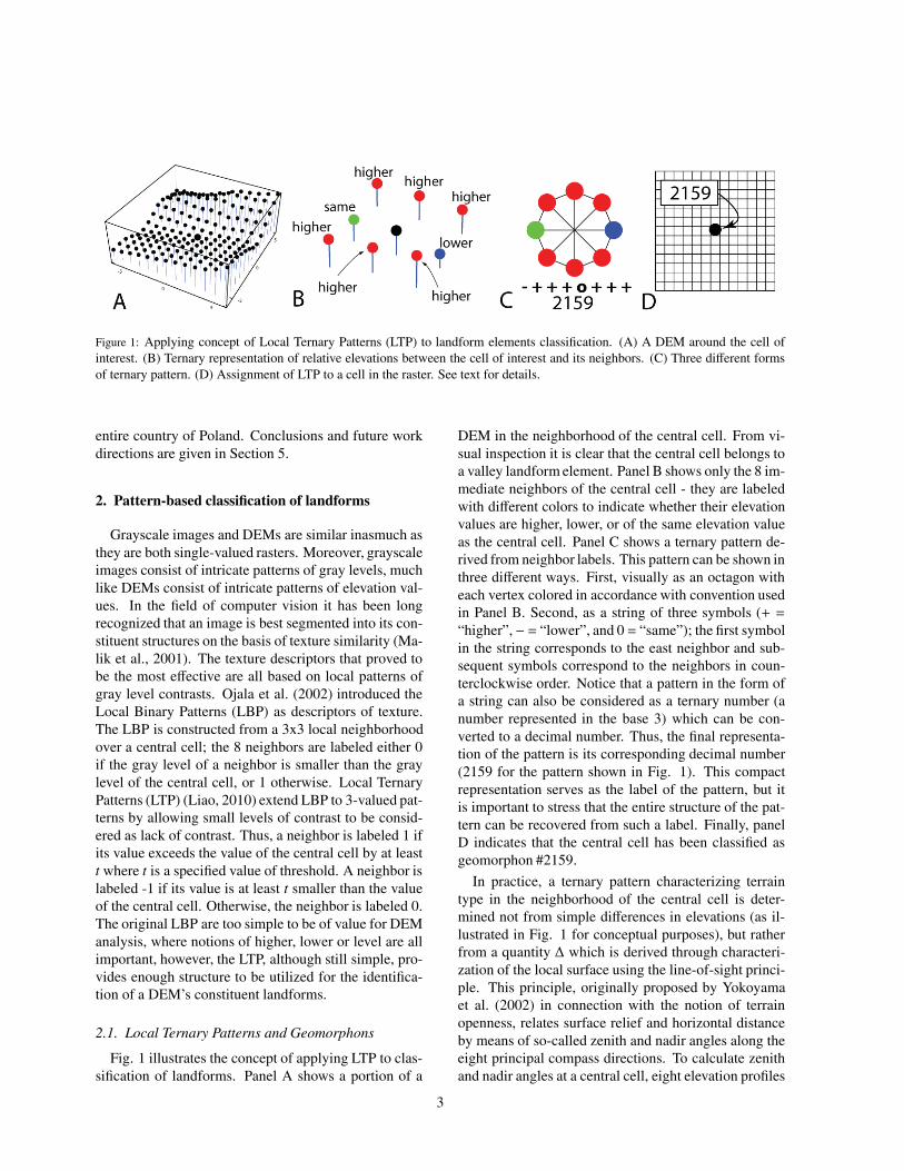
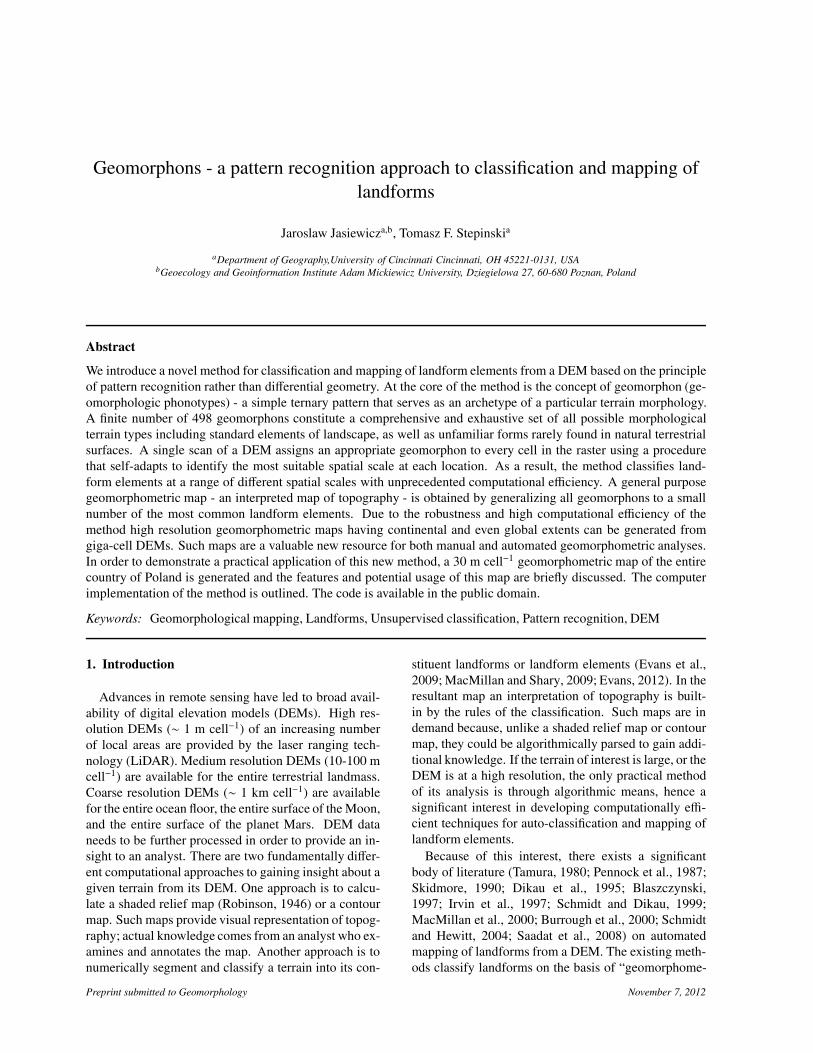
Figure 1: Applying concept of Local Ternary Patterns (LTP) to landform elements classification. (A) A DEM around the cell ofinterest. (B) Ternary representation of relative elevations between the cell of interest and its neighbors. (C) Three different formsof ternary pattern. (D) Assignment of LTP to a cell in the raster. See text for details.

entire country of Poland. Conclusions and future workdirections are given in Section 5.

2. Pattern-based classification of landforms

Grayscale images and DEMs are similar inasmuch asthey are both single-valued rasters. Moreover, grayscaleimages consist of intricate patterns of gray levels, muchlike DEMs consist of intricate patterns of elevation val-ues. In the field of computer vision it has been longrecognized that an image is best segmented into its con-stituent structures on the basis of texture similarity (Ma-lik et al., 2001). The texture descriptors that proved tobe the most effective are all based on local patterns ofgray level contrasts. Ojala et al. (2002) introduced theLocal Binary Patterns (LBP) as descriptors of texture.The LBP is constructed from a 3x3 local neighborhoodover a central cell; the 8 neighbors are labeled either 0if the gray level of a neighbor is smaller than the graylevel of the central cell, or 1 otherwise. Local TernaryPatterns (LTP) (Liao, 2010) extend LBP to 3-valued pat-terns by allowing small levels of contrast to be consid-ered as lack of contrast. Thus, a neighbor is labeled 1 ifits value exceeds the value of the central cell by at leastt where t is a specified value of threshold. A neighbor islabeled -1 if its value is at least t smaller than the valueof the central cell. Otherwise, the neighbor is labeled 0.The original LBP are too simple to be of value for DEManalysis, where notions of higher, lower or level are allimportant, however, the LTP, although still simple, pro-vides enough structure to be utilized for the identifica-tion of a DEM’s constituent landforms.

2.1. Local Ternary Patterns and Geomorphons

Fig. 1 illustrates the concept of applying LTP to clas-sification of landforms. Panel A shows a portion of a

DEM in the neighborhood of the central cell. From vi-sual inspection it is clear that the central cell belongs toa valley landform element. Panel B shows only the 8 im-mediate neighbors of the central cell - they are labeledwith different colors to indicate whether their elevationvalues are higher, lower, or of the same elevation valueas the central cell. Panel C shows a ternary pattern de-rived from neighbor labels. This pattern can be shown inthree different ways. First, visually as an octagon witheach vertex colored in accordance with convention usedin Panel B. Second, as a string of three symbols (+ =“higher”,− = “lower”, and 0 = “same”); the first symbolin the string corresponds to the east neighbor and sub-sequent symbols correspond to the neighbors in coun-terclockwise order. Notice that a pattern in the form ofa string can also be considered as a ternary number (anumber represented in the base 3) which can be con-verted to a decimal number. Thus, the final representa-tion of the pattern is its corresponding decimal number(2159 for the pattern shown in Fig. 1). This compactrepresentation serves as the label of the pattern, but itis important to stress that the entire structure of the pat-tern can be recovered from such a label. Finally, panelD indicates that the central cell has been classified asgeomorphon #2159.

In practice, a ternary pattern characterizing terraintype in the neighborhood of the central cell is deter-mined not from simple differences in elevations (as il-lustrated in Fig. 1 for conceptual purposes), but ratherfrom a quantity Δ which is derived through characteri-zation of the local surface using the line-of-sight princi-ple. This principle, originally proposed by Yokoyamaet al. (2002) in connection with the notion of terrainopenness, relates surface relief and horizontal distanceby means of so-called zenith and nadir angles along theeight principal compass directions. To calculate zenithand nadir angles at a central cell, eight elevation profiles

3

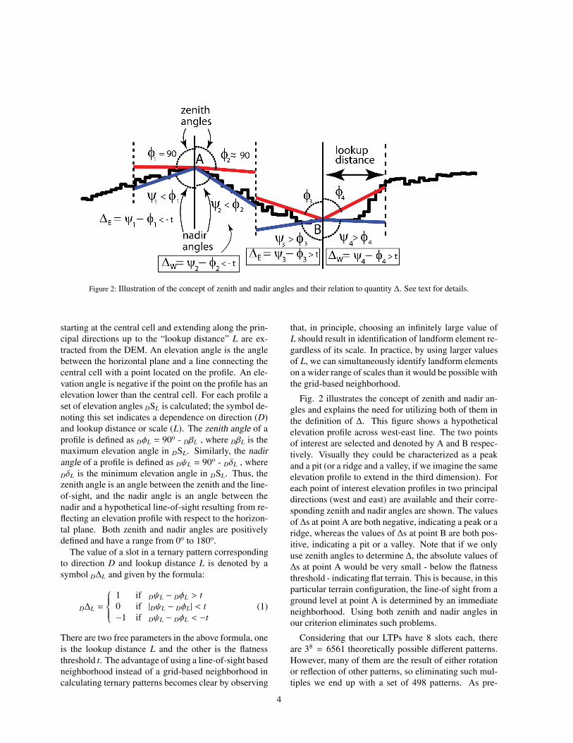
Figure 2: Illustration of the concept of zenith and nadir angles and their relation to quantity Δ. See text for details.

starting at the central cell and extending along the prin-cipal directions up to the “lookup distance” L are ex-tracted from the DEM. An elevation angle is the anglebetween the horizontal plane and a line connecting thecentral cell with a point located on the profile. An ele-vation angle is negative if the point on the profile has anelevation lower than the central cell. For each profile aset of elevation angles DSL is calculated; the symbol de-noting this set indicates a dependence on direction (D)and lookup distance or scale (L). The zenith angle of aprofile is defined as DφL = 90o - DβL , where DβL is themaximum elevation angle in DSL. Similarly, the nadirangle of a profile is defined as DψL = 90o - DδL , whereDδL is the minimum elevation angle in DSL. Thus, thezenith angle is an angle between the zenith and the line-of-sight, and the nadir angle is an angle between thenadir and a hypothetical line-of-sight resulting from re-flecting an elevation profile with respect to the horizon-tal plane. Both zenith and nadir angles are positivelydefined and have a range from 0o to 180o.

The value of a slot in a ternary pattern correspondingto direction D and lookup distance L is denoted by asymbol DΔL and given by the formula:

DΔL =

⎧⎪⎪⎪⎨⎪⎪⎪⎩

1 if DψL − DφL > t0 if |DψL − DφL| < t−1 if DψL − DφL < −t

(1)

There are two free parameters in the above formula, oneis the lookup distance L and the other is the flatnessthreshold t. The advantage of using a line-of-sight basedneighborhood instead of a grid-based neighborhood incalculating ternary patterns becomes clear by observing

that, in principle, choosing an infinitely large value ofL should result in identification of landform element re-gardless of its scale. In practice, by using larger valuesof L, we can simultaneously identify landform elementson a wider range of scales than it would be possible withthe grid-based neighborhood.

Fig. 2 illustrates the concept of zenith and nadir an-gles and explains the need for utilizing both of them inthe definition of Δ. This figure shows a hypotheticalelevation profile across west-east line. The two pointsof interest are selected and denoted by A and B respec-tively. Visually they could be characterized as a peakand a pit (or a ridge and a valley, if we imagine the sameelevation profile to extend in the third dimension). Foreach point of interest elevation profiles in two principaldirections (west and east) are available and their corre-sponding zenith and nadir angles are shown. The valuesof Δs at point A are both negative, indicating a peak or aridge, whereas the values of Δs at point B are both pos-itive, indicating a pit or a valley. Note that if we onlyuse zenith angles to determine Δ, the absolute values ofΔs at point A would be very small - below the flatnessthreshold - indicating flat terrain. This is because, in thisparticular terrain configuration, the line-of sight from aground level at point A is determined by an immediateneighborhood. Using both zenith and nadir angles inour criterion eliminates such problems.

Considering that our LTPs have 8 slots each, thereare 38 = 6561 theoretically possible different patterns.However, many of them are the result of either rotationor reflection of other patterns, so eliminating such mul-tiples we end up with a set of 498 patterns. As pre-

4

Figure 3: Symbolic 3D morphologies and their corresponding geomorphons (ternary patterns) for the 10 most common landformelements.

viously noticed, we refer to these patterns as geomor-phons. Geomorphons constitute a comprehensive andexhaustive set of idealized landform elements. We scana DEM cell-by-cell; at each cell we calculate valuesof DΔL for all eight principal directions. These valuesare inserted into equation (1) to obtain a ternary pat-tern and a decimal label of the pattern is stored in thecell corresponding to its location. In a typical fluviallandscape only about 60% of all theoretically possiblegeomorphons are actually present. Moreover, the abun-dances of different geomorphons are very uneven; the30 most common geomorphons account for 85% of allcells. The resulting landform element classification andits corresponding map is useful for tasks such as query-ing specific landform types in a study area. However,for a general purpose the number of landform elementsin a geomorphometric map needs to be reduced. Thisis achieved by grouping geomorphons into classes thatcorrespond to the most commonly recognizable land-form elements.

2.2. Mapping the most common landform elements

In a typical terrestrial landscape the most frequentand commonly recognizable geomorphons are: flat,peak, ridge, shoulder, spur, slope, hollow, footslope,valley, and pit. Their symbolic 3D morphologies andcorresponding LTPs are shown in Fig. 3. Note that thesecommon geomorphons are characterized by a low num-ber of transitions between ternary elements (1, 0,-1) intheir patterns. This reflects relatively high degree ofterrain autocorrelation (Fisher, 1998) even at the localscale. While traversing a LTP in order of principal di-rections a “transition” is a change in ternary element.Thus geomorphons flat, peak, and pit have 0 transitions,

as all ternary elements in their patterns are the same.Shoulder, spur, hollow, and valley have 2 transitions,while ridge, valley, and slope have 4 transitions. Geo-morphons with more complicated morphologies, for ex-ample, a “saddle,” have more transitions (up to 8) andare relatively rare.

In order to create a geomorphometric map contain-ing the top 10 most commonly recognizable geomor-phons in an exclusive and exhaustive fashion we needto reclassify the whole set of 498 geomorphons into10 selected forms. There is no a unique reclassifica-tion formula able to accomplish this task perfectly. Anyformula will result in a small number of cells that aremisclassified due to the uncertainty of how to reclassifysome rare geomorphons into the common forms. Wehave chosen a reclassification formula based on a partic-ular lookup table constructed on the basis of similaritybetween ternary patterns representing the geomorphons;patterns are similar if they have similar number of dif-ferent ternary elements. Fig. 4 shows our lookup table;rows indicate the number of (-1) elements in the pat-tern and columns indicate the number of (1) elementsin the pattern. For example, the archetypal “flat” ge-omorphon, like the one shown on Fig. 3, consists ex-clusively of (0) ternary elements therefore its numberof (-1) elements is zero and its number of (1) elementsis also zero. This geomorphon will fall in the upperleft corner of the lookup table. We have also chosento classify as “flat” those geomorphons which departslightly from this archetype, as indicated by additionalfour “flat” slots in the lookup table.

In order to further explain the idea behind the lookuptable Fig. 5 shows a sample of terrain dominated by avalley. We have calculated geomorphons at four differ-

5

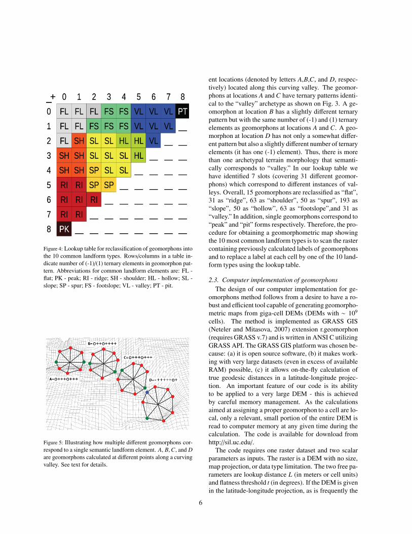
Figure 4: Lookup table for reclassification of geomorphons intothe 10 common landform types. Rows/columns in a table in-dicate number of (-1)/(1) ternary elements in geomorphon pat-tern. Abbreviations for common landform elements are: FL -flat; PK - peak; RI - ridge; SH - shoulder; HL - hollow; SL -slope; SP - spur; FS - footslope; VL - valley; PT - pit.

Figure 5: Illustrating how multiple different geomorphons cor-respond to a single semantic landform element. A, B, C, and Dare geomorphons calculated at different points along a curvingvalley. See text for details.

ent locations (denoted by letters A,B,C, and D, respec-tively) located along this curving valley. The geomor-phons at locations A and C have ternary patterns identi-cal to the “valley” archetype as shown on Fig. 3. A ge-omorphon at location B has a slightly different ternarypattern but with the same number of (-1) and (1) ternaryelements as geomorphons at locations A and C. A geo-morphon at location D has not only a somewhat differ-ent pattern but also a slightly different number of ternaryelements (it has one (-1) element). Thus, there is morethan one archetypal terrain morphology that semanti-cally corresponds to “valley.” In our lookup table wehave identified 7 slots (covering 31 different geomor-phons) which correspond to different instances of val-leys. Overall, 15 geomorphons are reclassified as “flat”,31 as “ridge”, 63 as “shoulder”, 50 as “spur”, 193 as“slope”, 50 as “hollow”, 63 as “footslope”,and 31 as“valley.” In addition, single geomorphons correspond to“peak” and “pit” forms respectively. Therefore, the pro-cedure for obtaining a geomorphometric map showingthe 10 most common landform types is to scan the rastercontaining previously calculated labels of geomorphonsand to replace a label at each cell by one of the 10 land-form types using the lookup table.

2.3. Computer implementation of geomorphonsThe design of our computer implementation for ge-

omorphons method follows from a desire to have a ro-bust and efficient tool capable of generating geomorpho-metric maps from giga-cell DEMs (DEMs with ∼ 109

cells). The method is implemented as GRASS GIS(Neteler and Mitasova, 2007) extension r.geomorphon(requires GRASS v.7) and is written in ANSI C utilizingGRASS API. The GRASS GIS platform was chosen be-cause: (a) it is open source software, (b) it makes work-ing with very large datasets (even in excess of availableRAM) possible, (c) it allows on-the-fly calculation oftrue geodesic distances in a latitude-longitude projec-tion. An important feature of our code is its abilityto be applied to a very large DEM - this is achievedby careful memory management. As the calculationsaimed at assigning a proper geomorphon to a cell are lo-cal, only a relevant, small portion of the entire DEM isread to computer memory at any given time during thecalculation. The code is available for download fromhttp://sil.uc.edu/.

The code requires one raster dataset and two scalarparameters as inputs. The raster is a DEM with no size,map projection, or data type limitation. The two free pa-rameters are lookup distance L (in meters or cell units)and flatness threshold t (in degrees). If the DEM is givenin the latitude-longitude projection, as is frequently the

6

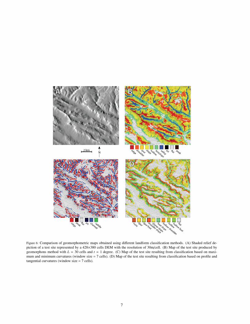
Figure 6: Comparison of geomorphometric maps obtained using different landform classification methods. (A) Shaded relief de-piction of a test site represented by a 428×380 cells DEM with the resolution of 30m/cell. (B) Map of the test site produced bygeomorphons method with L = 30 cells and t = 1 degree. (C) Map of the test site resulting from classification based on maxi-mum and minimum curvatures (window size = 7 cells). (D) Map of the test site resulting from classification based on profile andtangential curvatures (window size = 7 cells).

7

case for global or continental-size datasets, and L isgiven in cell units, an actual metric lookup distance isset automatically using a uniform, latitudinal metric di-mension of a raster cell. The metric value of L is thenapplied over the entire extent of the DEM. The code re-turns two raster outputs, both with the same dimensionsas the input DEM. The first raster stores decimal labelsof geomorphons assigned to each cell; this output is tan-tamount to a map showing the spatial distribution of all(up to 498) geomorphons; it can be utilized to query thedataset for a highly specific landform type. The secondraster stores the geomorphometric map - the map of the10 most common landform elements - the lookup tabledefined in section 2.2 is used to obtain this output.

3. Geomorphometric maps: geomorphons vs. dif-ferential geometry

As mentioned in Section 1, most methods for the au-tomated mapping of landform elements rely on differen-tial geometry. In such methods a landform element of alocal surface is determined from the signs and values ofthe slope and curvature of a surface (Dikau et al., 1995;Wood, 1996). This popular method is sufficient for rel-atively small rasters, but its computational efficiency istoo low for its application to giga-cell DEMs. These in-efficiencies stem from the following: (a) a necessity tocalculate quadratic approximation to the surface at eachcell; (b) relatively complex algorithm for assignment ofall major landform elements; (c) a necessity to apply amulti-scale approach. The geomorphons-based methoddoes not have such built-in computational inefficienciesand can be used for classification of giga-cell DEMs.

A map resulting from reclassification of all 498 ge-omorphons into the 10 most common forms depicts allimportant landform elements in a single map. In con-trast, popular classification schemes based on curvature-derived features depict only a subset of important land-form elements. In order to illustrate this point we com-pare the map obtained using geomorphons with themaps resulting from the two most common curvature-derived classification schemes.

The first such scheme (Wood, 1996) classifies thesurface into six landform elements: peak, ridge, plain(which we refer to as flat), saddle, channel, and pit.This classification does not include various types ofslopes. In order to classify the slopes, a differentscheme (Dikau et al., 1995), based on the signs of pro-file and tangential curvatures, classifies all non-zerogradient parts of the surface into nine landform ele-ments: nose, shoulder slope, hollow shoulder, spur,

planar slope, hollow, spur foot, foot slope, and hol-low foot (Dikau et al., 1995; Schmidt and Andrew,2005). All areas of zero gradient are grouped into a sin-gle additional landform element, which we refer to as“flat,”. We calculated the two curvature-based classifi-cation schemes using the GRASS module r.param.scalewhich is based on work by Wood (Wood, 1996). Thismodule implements Wood’s classification scheme di-rectly. The Dikau’s scheme was implemented usingprofile and cross-sectional curvatures as calculated byr.param.scale. In both cases we used the following pa-rameters: slope tolerance equal to 1 degree, curvaturetolerance equal to 0.0001, size of processing windowsequal to 7 pixels.

Fig. 6 shows a comparison of the three classificationschemes. Panel A depicts the topography of the testsite through a shaded relief map; the test site was ob-tained using a 428×380 cell DEM with resolution of 30m cell−1. Panel B shows a map generated by our geo-morphon methods. Visual comparison of this map withthe shaded relief confirms that our method classifies to-pography well, with all important landform elementspresent and corresponding to what is seen in the shadedrelief. Panels C and D show maps generated by Wood’sand Dikau’s schemes, respectively. Visual comparisonof these maps with the shaded relief indicates that thetwo methods delineate well their respective landform el-ements, but each map by itself is incomplete and doesnot depict the entire terrain in a satisfactory manner.Of course, it is possible to merge (Schmidt and Hewitt,2004) Wood’s and Dikau’s classification schemes into asingle scheme showing all 15 landform types. However,in order to perform such merged scheme, Schmidt andHewitt had to resort to fuzzy classification technique(at high computational cost) to take into account con-siderable uncertainty in the slope tolerance parameter.On the other hand, our geomorphons technique yields acomplete and satisfactory classification of landform el-ements at relatively low computational cost.

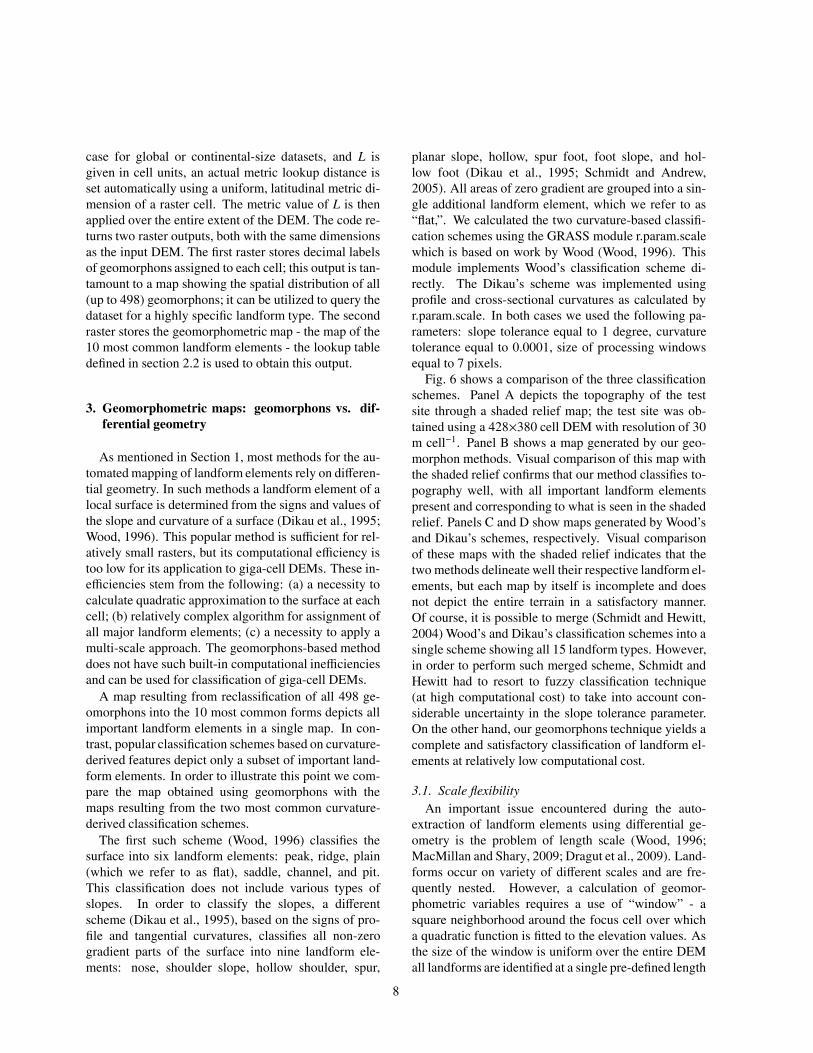
3.1. Scale flexibilityAn important issue encountered during the auto-

extraction of landform elements using differential ge-ometry is the problem of length scale (Wood, 1996;MacMillan and Shary, 2009; Dragut et al., 2009). Land-forms occur on variety of different scales and are fre-quently nested. However, a calculation of geomor-phometric variables requires a use of “window” - asquare neighborhood around the focus cell over whicha quadratic function is fitted to the elevation values. Asthe size of the window is uniform over the entire DEMall landforms are identified at a single pre-defined length

8

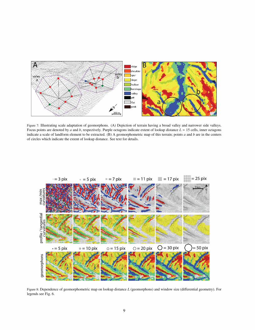
Figure 7: Illustrating scale adaptation of geomorphons. (A) Depiction of terrain having a broad valley and narrower side valleys.Focus points are denoted by a and b, respectively. Purple octagons indicate extent of lookup distance L = 15 cells, inner octagonsindicate a scale of landform element to be extracted. (B) A geomorphometric map of this terrain; points a and b are in the centersof circles which indicate the extent of lookup distance. See text for details.

Figure 8: Dependence of geomorphometric map on lookup distance L (geomorphons) and window size (differential geometry). Forlegends see Fig. 6.

9

scale. A change in window size results in a differentmap. In order to address this problem Wood (2002),Fisher et al. (2004), and Schmidt and Hewitt (2004) pro-posed to use a variety of different window sizes and toassign a dominant landform type to each cell. From acomputational point of view this is a very inefficient so-lution as it requires a calculation of multiple maps (eachone at a different scale) before the final map can be ob-tained.

The geomorphons method does not use a fixed-sizeneighborhood, instead the size and the shape of a neigh-borhood from which the landform element is deter-mined adjusts automatically to the geometry of the lo-cal terrain (see section 2.1). This allows our method todetermine the most appropriate landform element (andits scale) in a single scan of a DEM. Fig. 7 illustrateshow geomorphons adapt to the actual scale of local ter-rain. Panel A depicts a terrain dominated by a relativelybroad valley which also has few narrower side valleys.We have chosen two specific points (cells); point a is lo-cated in the middle of the broad valley and point b is lo-cated in one of the narrow valleys. The purple octagons(having the same size at points a and b) show the ex-tent to which we examine the terrain; this is determinedby the lookup distance L (see section 2.1). The valueof L determines the maximum scale at which we canfind the landform element; it needs to be set to a rela-tively large value in order for the map to show landformelements at a broad range of scales. The inner, irreg-ular octagons (having different sizes at points a and b)are determined by the line-of-sight principle in the eightprincipal compass directions - they determine the actualscale over which the landform element is detected. Atboth points the ultimate landform element detected is avalley (lookup table shown in Fig. 4 assigns both pat-terns to valley type), but the detection at point a is madeover a larger scale and the detection at point b is madeover a smaller scale. Panel B shows a geomorphometricmap of terrain depicted in panel A; points a and b arelocated in the middle of the circles that indicate the sizeof L. The map correctly delineates valleys (as well asother landform elements) at range of scales.

A desirable property of geomorphons method is thatmaps created with different values of lookup distanceL quickly converge with increasing value of L. Thismeans that although L is a free parameter, it can be set toan optimal value (this value may depend on the resolu-tion of the original DEM and spatial variability of land-form scales across its extent) which is large enough tomap landforms at most relevant scales but small enoughfor rapid computations (increasing the value of L in-creases computational cost). Fig. 8 demonstrates such

convergence for a small DEM having resolution of 30m cell−1. We have created geomorphometric maps us-ing values of L equal to 5, 10, 15, 20, 30, and 50 cellsrespectively. It is clear that L = 20 cells is sufficientto map this particular type of landscape at that resolu-tion; further increasing the value of L would increasethe cost of calculation without meaningful change to themap. There is no equivalent “optimal” window size forthe methods based on differential geometry; increasingthe window size completely changes the character of themap (Fig. 8), so the only way to get a multi-resolutionmap is to follow a computationally costly multi-windowapproach (Wood, 2002; Fisher et al., 2004; Schmidt andHewitt, 2004). Note, however, that even the multi-window approach does not guarantee a unique map asthe result may depend on a particular choice of windowsizes.

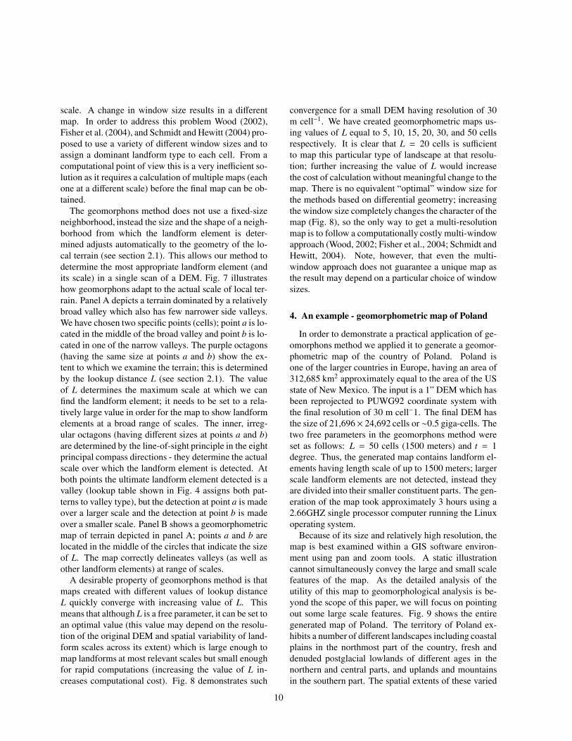
4. An example - geomorphometric map of Poland

In order to demonstrate a practical application of ge-omorphons method we applied it to generate a geomor-phometric map of the country of Poland. Poland isone of the larger countries in Europe, having an area of312,685 km2 approximately equal to the area of the USstate of New Mexico. The input is a 1” DEM which hasbeen reprojected to PUWG92 coordinate system withthe final resolution of 30 m cell−1. The final DEM hasthe size of 21,696× 24,692 cells or ∼0.5 giga-cells. Thetwo free parameters in the geomorphons method wereset as follows: L = 50 cells (1500 meters) and t = 1degree. Thus, the generated map contains landform el-ements having length scale of up to 1500 meters; largerscale landform elements are not detected, instead theyare divided into their smaller constituent parts. The gen-eration of the map took approximately 3 hours using a2.66GHZ single processor computer running the Linuxoperating system.

Because of its size and relatively high resolution, themap is best examined within a GIS software environ-ment using pan and zoom tools. A static illustrationcannot simultaneously convey the large and small scalefeatures of the map. As the detailed analysis of theutility of this map to geomorphological analysis is be-yond the scope of this paper, we will focus on pointingout some large scale features. Fig. 9 shows the entiregenerated map of Poland. The territory of Poland ex-hibits a number of different landscapes including coastalplains in the northmost part of the country, fresh anddenuded postglacial lowlands of different ages in thenorthern and central parts, and uplands and mountainsin the southern part. The spatial extents of these varied

10

Figure 9: Geomorphometric map of Poland generated using the geomorphons method with L = 1500 m and t = 1 degree. Whiteletters indicate different physigraphic units: W - poorly denuded young postglacial morainic and sandur plains of Weichselian age;L - moderately to strongly denuded old postglacial plains of Saalian and Elsterian age; g - maximum extend of Weichselian (last)glaciation; U - uplands, M -mountains.

11

Figure 10: Geomorphometric map vs. shaded relief map. (A) Shaded relief map of North-Eastern Poland. (B) Geomorphometricmap of North-Eastern Poland. Blue line indicates maximum extend of the last glaciation according to Marks (2005).

12

landscapes are identifiable on Fig. 9 as different patternsof colors representing major landform elements. De-lineation of these patterns coincides with physiographicpartition of Poland (Kondracki, 2002).

One possible application of a geomorphometric mapis for visual delineation of landscape units. We sub-mit that a geomorphometric map - the interpreted mapof topography - is a better tool for such analysis than amap of a shaded relief - a 3D visualization of topogra-phy. Fig. 10 shows a North-Eastern portion of Polandin the form of shadow relief and a geomorphometricmap respectively. This part of Poland is a lowland cov-ered by glacial deposits. The northern portion of thisregion (above the blue line) results from glacial mor-phogenesis during the last glaciation and is poorly de-nuded, whereas the southern portion of this region (be-low the blue line) results from glacial activity duringthe previous glaciation and has been extensive denudedin periglacial condition during the Weichselian (Dylik,1967; Rotnicki, 1974; Starkel, 1986). As a result, thelandscape of the northern portion of the region is char-acterized by sharp incisions leading to the dominationof ridge and valley landform elements (prevalence ofred and blue colors) and relative paucity of shoulder andfootslope landform elements (suppression of green andorange colors). On the other hand, the landscape of thesouthern portion of the region is characterized by broadincisions leading to domination of shoulder and foots-lope landform elements (green and orange colors) overridge and valley landform elements (red and blue col-ors). Thus, the two different landscapes are easy to rec-ognize on the geomorphometric map as the two areascontain visibly different color patterns (Fig. 1B), but aredifficult to recognize on the basis of the shaded reliefalone (Fig. 1A).

5. Conclusions and future work

Geomorphons offer a novel perspective on how to ap-proach quantitative terrain analysis. The method grewfrom our desire to develop a robust and computation-ally efficient tool for classification of landforms fromgiga-cell DEMs. It became clear that standard methods,based on geomorphometric variables, fall short of thecomputational efficiency required to tackle such largeDEMs.

Geomorphons represent a paradigm shift in DEMclassification. First, the method is underpinned by prin-ciples of machine vision rather than differential geom-etry. Second, it classifies landforms at different spatialscales simultaneously. Both of these innovations con-tribute to the robustness and efficiency of geomorphons.

In the machine vision approach the landforms are iden-tified holistically from the pattern of a local terrain. Thekey breakthrough was the realization that a finite num-ber of elementary patterns is sufficient to encapsulateall possible forms of terrain. Another breakthrough wasthe realization that a local elementary form can be de-termined at a locally optimal spatial scale. Scale self-adaptation contributes to computational efficiency be-cause only a single scan of the DEM is required to de-tect landforms at a range of spatial scales. In this paperwe have described the details of geomorphons methodand demonstrated its advantages in terms of robustnessas well as in terms of computational efficiency.

Future work on the geomorphons algorithm will con-centrate on two main extensions. First, we will ex-periment with the addition of a third free parameter -exclusion distance. A function of exclusion distanceis to further restrict a range of scales at which land-form elements are identified. The lookup distance Ldetermines the maximum scale of a landform element,but the present implementation of geomorphons methoddoes not have a parameter to set a minimum scale of anelement. An exclusion distance, which sets the min-imum scale of a landform element, is meant to pre-vent the immediate neighborhood of a focus locationfrom determining an element at that location. It of-fers flexibility in filtering out terrain forms at scales thatare too small to be of interest. Furthermore, a combi-nation of lookup and exclusion distances can be usedto identify only landform elements at narrowly definedspatial scales. Secondly, we will experiment with dif-ferent lookup tables,which will make the geomorphonsmethod more appropriate for exotic terrains, such asMartian and lunar surfaces or the surface of the oceanfloor. Future research will also identify novel practicalapplications for giga-cell geomorphometricmaps gener-ated using our method. In particular, these maps couldprovide an input for pattern-based query tool capable ofidentifying all local landscapes similar to a given ref-erence. A query tool could also be used for the com-prehensive assessment of synthetic landscapes (Howardand Tierney, 2012).

Acknowledgments. This work was supported by theNational Science Foundation under Grant IIS-1103684.

References

Adediran, A., Parcharidis, I., Poscolieri, M., Pavlopoulos, K., 2004.Computer-assisted discrimination of morphological units on north-central Crete (Greece) by applying multivariate statistics to localrelief gradients. Geomorphology 58, 357–370.

13

Blaszczynski, J., 1997. Landform characterization with geographicinformation systems. Photogrammetric Engineering and RemoteSensing 63, 183–191.

Brown, D., Lusch, D., Duda, K., 1998. Supervised classification oftypes of glaciated landscapes using digital elevation data. Geomor-phology 21, 233–250.

Burrough, P., van Gaans, P., MacMillan, R., 2000. High-resolutionlandform classification using fuzzy k-means. Fuzzy Sets and Sys-tems 113, 37–52.

Datta, R., Joshi, D., Li, J., Wang, J. Z., 2008. Image Retrieval: Ideas,Influences, and Trends of the New Age. ACM Computing Surveys40, 1–60.

Dikau, R., Brabb, E., Mark, R., 1995. Morphometric landform anal-ysis of New Mexico. Zeitschrift fur Geomorphologie Supplement101, 109–126.

Dragut, L., Blaschke, T., 2006. Automated classification of landformelements using object-based image analysis. Geomorphology 81,330–344.

Dragut, L., Blaschke, T., 2008. Terrain Segmentation and Classifica-tion using SRTM Data. In: Zhou, Q., Lees, B., Tang, G. (Eds.),Advances in Digital Terrain Analysis. Springer Verlag, pp. 141–158.

Dragut, L., Eisank, C., 2012. Automated object-based classificationof topography from SRTM data. Geomorphology 141-142, 21–23.

Dragut, L., Eisank, C., Strasser, T., Blaschke, T., 2009. A comparisonof methods to incorporate scale in Geomorphometry. In: Purves,R., Molnar, P., Gruber, S. (Eds.), Proceedings of Geomorphometry2009. Zurich, Switzerland, 31 August - 2 September, 2009. pp.133–139.

Dylik, J., 1967. Solifluxion, congelifluxion and related slope pro-cesses. Geografiska Annaler. Series A, Physical Geography 49,167–177.

Evans, I., 1972. General geomorphometry, derivatives of altitude, anddescriptive statistics. In: Chorley, R. J. (Ed.), Spatial analysis ingeomorphology. Methuen, pp. 17–90.

Evans, I., Mar. 2012. Geomorphometry and landform mapping: whatis a landform? Geomorphology 137, 94–106.

Evans, I., Hengl, T., Gorsevski, P., 2009. Applications in geomorphol-ogy. In: Hengl, T., Reuter, H. (Eds.), Geomorphometry, Concepts,Software, Application. Elsevier, Ch. 22, pp. 497–525.

Fisher, P., 1998. Improved Modeling of Elevation Error with Geo-statistics. Geoinformatica 2, 215–233.

Fisher, P., Wood, J., Cheng, T., 2004. Where is Helvellyn? Fuzzinessof multi-scale landscape morphometry. Transactions of the Insti-tute of British Geographers 29, 106–128.

Gallant, A. L., Brown, D. D., Hoffer, R. M., 2005. Automated Map-ping of Hammond’s Landforms. IEEE Geoscience and RemoteSensing Letters 2, 384–288.

Ghosh, S., Stepinski, T. F., R.Vilalta, 2009. Automatic Annotation ofPlanetary Surfaces With Geomorphic Labels. IEEE Transactionson Geoscience and Remote Sensing 48, 175 – 185.

Hengl, T., Rossiter, D. G., 2003. Supervised Landform Classificationto Enhance and Replace Photo-Interpretation in Semi-Detailed SoilSurvey. Soil Science Society of America Journal 67, 1810.

Howard, A., Tierney, H., Mar. 2012. Taking the measure of a land-scape: Comparing a simulated and natural landcape in the Virginiacoastal plain. Geomorphology 137, 27–40.

Irvin, B., Ventura, S., Slater, B., 1997. Fuzzy and isodata classificationof landform elements from digital terrain data in Pleasant Valley,Wisconsin. Geoderma 77, 137–154.

Iwahashi, J., Pike, R., 2007. Automated classifications of topogra-phy from DEMs by an unsupervised nested-means algorithm anda three-part geometric signature. Geomorphology 86, 409–440.

Julesz, B., 1981. Textons, the elements of texture perception, and theirinteractions. Nature 290, 91–97.

Julesz, B., 1984. A brief outline of the texton theory of human vision.Trends in Neurosciences 7, 41–45.

Kondracki, J., 2002. Geografia regionalna Polski, 3rd Edition.Wydawnictwo Naukowe PWN, Warszawa.

Lee, J., 1991. Analyses of visibility sites on topographic surfaces. In-ternational Journal of Geographical Information 5, 413–429.

Liao, W.-H., Aug. 2010. Region Description Using Extended LocalTernary Patterns. 2010 20th International Conference on PatternRecognition, 1003–1006.

MacMillan, R., Jones, R., McNabb, D., 2004. Defining a hierarchy ofspatial entities for environmental analysis and modeling using dig-ital elevation models (DEMs). Computers, Environment and UrbanSystems 28, 175–200.

MacMillan, R., Pettapiece, W., Nolan, S., Goddard, T., 2000. Ageneric procedure for automatically segmenting landforms intolandform elements using DEMs, heuristic rules and fuzzy logic.Fuzzy Sets and Systems 113, 81–109.

MacMillan, R., Shary, P., 2009. Landforms and landform elements ingeomorphometry. In: Hengl, T., Reuter, H. (Eds.), Geomorphome-try, Concepts, Software, Application. Elsevier, Ch. 9, pp. 227–275.

Malik, J., Belongie, S., Leung, T., Shi, J., 2001. Contour and TextureAnalysis for Image Segmentation. International Journal of Com-puter Vision 43, 7–27.

Marks, L., 2005. Pleistocene glacial limits in the territory of Poland.Przegld Geologiczny 53 (10), 988–993.

Minar, J., Evans, I., 2008. Elementary forms for land surface segmen-tation: The theoretical basis of terrain analysis and geomorpholog-ical mapping. Geomorphology 95, 236–259.

Nagy, G., 1994. Terrain visibility. Computers & Graphics 18, 763–773.

Neteler, M., Mitasova, H., 2007. Open source GIS: a GRASS GISapproach, 3rd Edition. Springer, New York.

Ojala, T., Pietikainen, M., Maenpaa, T., 2002. Multiresolution gray-scale and rotation invariant texture classification with local binarypatterns. IEEE Transactions on Pattern Analysis and Machine In-telligence 24, 971–987.

Olaya, V., 2009. Basic land-surface parameters. In: Hengl, T., Reuter,H. (Eds.), Geomorphometry, Concepts, Software, Application. El-sevier, Ch. 6, pp. 141–169.

Pennock, D., Zebarth, B., De Jong, E., 1987. Landform classificationand soil distribution in hummocky terrain, Saskatchewan, Canada.Geoderma 40, 297–315.

Pike, R., 1988. The geometric signature: quantifying landslide-terraintypes from digital elevation models. Mathematical Geology 20,491–511.

Prima, O. D. A., Echigo, A., Yokoyama, R., Yoshida, T., 2006. Su-pervised landform classification of Northeast Honshu from DEM-derived thematic maps. Geomorphology 78, 373–386.

Robinson, A., 1946. A method for producing shaded relief from arealslope data. Annals of the Association of American Geographers36, 248–252.

Rotnicki, K., 1974. Slope development of Riss Glaciation endmoraines during the Wurm; its morphological and geological con-sequences. Questiones Geographicae 1, 109–139.

Saadat, H., Bonnell, R., Sharifi, F., Mehuys, G., Namdar, M., Ale-Ebrahim, S., 2008. Landform classification from a digital elevationmodel and satellite imagery. Geomorphology 100, 453–464.

Schmidt, J., Andrew, R., 2005. Multi-scale landform characterization.Area 37, 341–350.

Schmidt, J., Dikau, R., 1999. Extracting geomorphometric attributesand objects from digital elevation modelssemantics, methods, fu-ture needs. In: Dikau, R., Saurer, H. (Ed.), GIS for Earth SurfaceSystems. Gebrueder Borntraeger, Berlin, pp. 154–173.

Schmidt, J., Hewitt, A., 2004. Fuzzy land element classification fromDTMs based on geometry and terrain position. Geoderma 121,

14

243–256.Skidmore, A., 1990. Terrain position as mapped from a gridded dig-

ital elevation model. International Journal of Geographical Infor-mation 4, 37–41.

Starkel, L., 1986. The role of the Vistulian and Holocene in the trans-formation of the relief of Poland. Biuletyn Peryglacjalny 31, 261–273.

Stepinski, T. F., Bagaria, C., 2009. Segmentation-Based UnsupervisedTerrain Classification for Generation of Physiographic Maps. IEEEGeoscience and Remote Sensing Letters 6, 733 – 737.

Tamura, T., 1980. Multiscale Landform ClassificationStudy in the Hills of Japan: Part I: Device of a Mul-tiscale Landform Classification System. Tech. rep.,http://ir.library.tohoku.ac.jp/re/handle/10097/45094.

van Asselen, S., Seijmonsbergen, A. C., 2006. Expert-Driven Semi-Automated Geomorphological Mapping for a Mountainous AreaUsing a Laser DTM. Geomorphology 78, 309–320.

Wood, J., 1996. The geomorphological characterisation of digi-tal elevation models. Ph.D. thesis, University of Leicester, UKhttp://www.soi.city.ac.uk/ jwo/phd.

Wood, J., 2002. LandSerf: visualisation and analysis of terrain modelshttp://www.landserf.org.

Yokoyama, R., Shlrasawa, M., Pike, R. J., 2002. Visualizing Topogra-phy by Openness:A New Application of Image Processing to Dig-ital Elevation Models. Photogrammetric Engineering & RemoteSensing 68, 257–265.

15