geometryofimageformation - cmpcmp.felk.cvut.cz/cmp/courses/xe33pvr/ws20072008/lectures/...32/47...

Talk Outline

� Pinhole model

� Camera parameters

� Estimation of the parameters—Camera calibration

Geometry of image formationTomáš Svoboda, [email protected]

Czech Technical University in Prague, Center for Machine Perceptionhttp://cmp.felk.cvut.cz

Last update: November 3, 2008

http://cmp.felk.cvut.cz/~svoboda

http://cmp.felk.cvut.cz

2/47Motivation

� parallel lines

� window sizes

� image units

� distance from the camera


3/47What will we learn

� how does the 3D world project to 2Dimage plane?

� how is a camera modeled?

� how can we estimate the camera model?


4/47Pinhole camera

1

1http://en.wikipedia.org/wiki/Pinhole camera


http://en.wikipedia.org/wiki/Pinhole_camera

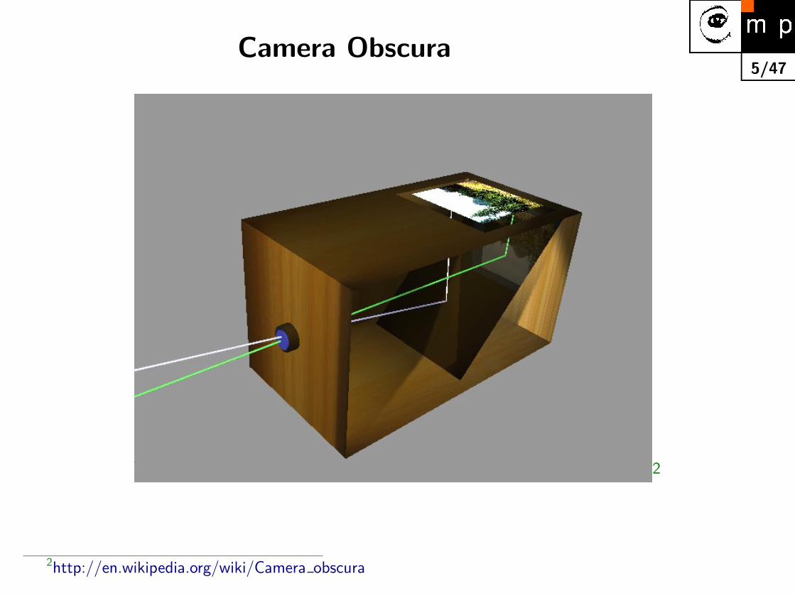
5/47Camera Obscura

2

2http://en.wikipedia.org/wiki/Camera obscura


http://en.wikipedia.org/wiki/Camera_obscura

6/47Camera Obscura — room-sized

3

Used by the art department at the UNC at Chapel Hill

3http://en.wikipedia.org/wiki/Camera obscura


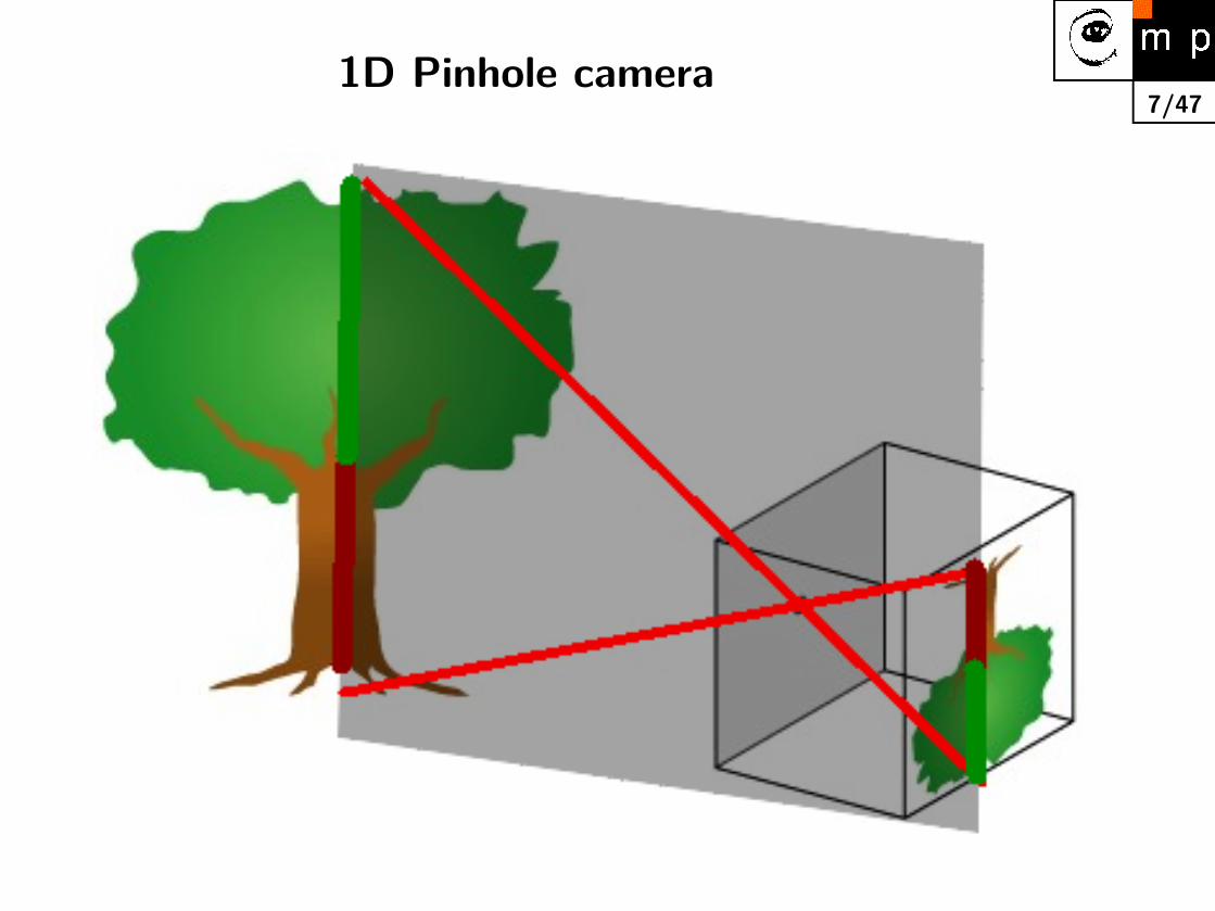
http://en.wikipedia.org/wiki/Camera_obscura

7/471D Pinhole camera


8/471D Pinhole camera projects 2D to 1D

Z1

Z2

Z3

Z1

x

z optical axis

imag

epl

ane

imag

epl

ane

−f

X1

x1

C

x1−f = X1

Z1

x1 = −f X1Z1


9/47Problems with perspective I

Z1

Z2

Z3

Z1

Z2

x

z optical axis

imag

epl

ane

imag

epl

ane

−f

X1 X2

x1

x2C

X1 = X2x1 6= x2


10/47Problems with perspective II

Z2

Z3

Z2

Z3

x

z optical axis

imag

epl

ane

imag

epl

ane

−f

X2

X3

x2x3C

X2 6= X3x2 = x3


11/47Get rid of the (−) sign

Z1

Z2

Z3

x

z optical axis

imag

epl

ane

imag

epl

ane

imag

epl

ane

imag

epl

ane

−f

f

X1 X2

X3

x1

x2x3

x1x2x3

C


12/47

How does the 3D worldproject to the 2D image plane?


13/47A 3D point X in a world coordinate system

X

X

X

X

X

X

X

X

X

X

x y

z

[0, 0, 0]

C

X


14/47A pinhole camera observes a scene

X

X

X

X

X

X

X

X

X

X

x y

z

[0, 0, 0]

C

X


15/47Point X projects to the image plane, point x

X

X

X

X

X

X

X

X

X

X

x y

z

[0, 0, 0]

C

x

X


16/47Scene projection

X

X

X

X

X

X

X

X

X

X

x y

z

[0, 0, 0]

C

x


17/47Scene projection

x y

z

[0, 0, 0]X

X

X

X

X

X

X

X

X

X

C


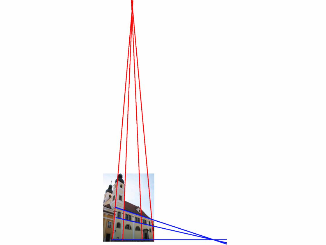
18/473D Scene projection – observations

C� 3D lines project to 2D lines� but the angles change, parallel lines are no more parallel.� area ratios change, note the front and backside of the house


19/47

Put the sketches into equations


20/473D → 2D Projection

We remember that: x = [fXZ ,fYZ ]>

[x1

]'

fX

fY

Z

[

x1

]'

f 0f 0

1 0

[ X1

]

Use the homegeneous coordinates4

λ[1×1]x[3×1] = K[3×3]

[I|0

]X[4×1]

but . . .C

x

X

4for the notation conventions, see the talk notes


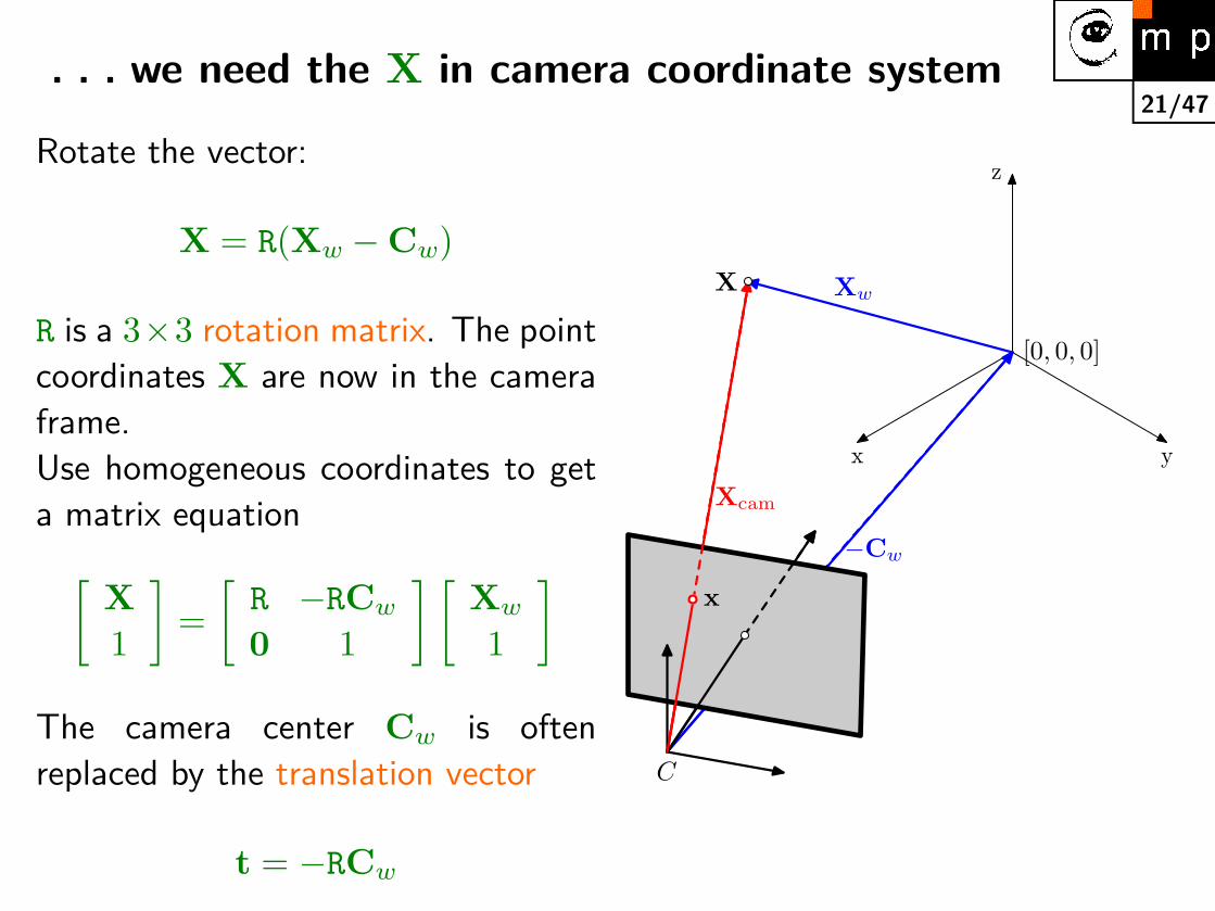
http://cmp.felk.cvut.cz/cmp/courses/XE33PVR/WS20072008/Lectures/Geometry/pinhole-note.pdf

21/47. . . we need the X in camera coordinate system

Rotate the vector:

X = R(Xw −Cw)

R is a 3×3 rotation matrix. The pointcoordinates X are now in the cameraframe.Use homogeneous coordinates to geta matrix equation[

X1

]=[R −RCw

0 1

] [Xw

1

]The camera center Cw is oftenreplaced by the translation vector

t = −RCw

x y

z

[0, 0, 0]

C

x

X Xw

−Cw

Xcam


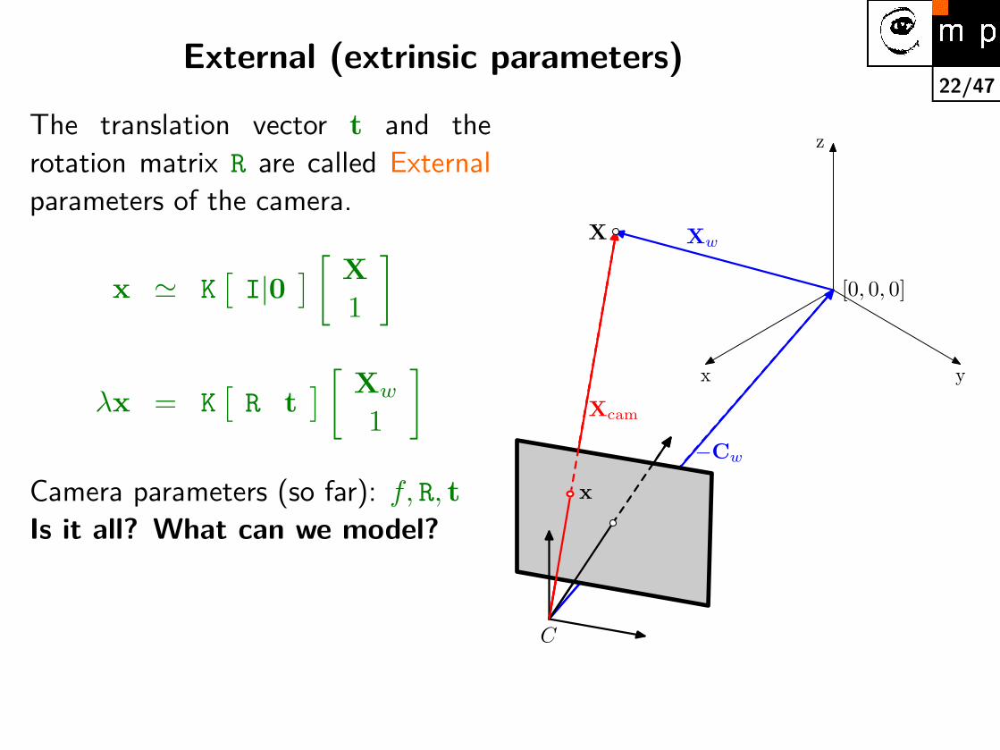
22/47External (extrinsic parameters)

The translation vector t and therotation matrix R are called Externalparameters of the camera.

x ' K[I|0

] [ X1

]

λx = K[R t

] [ Xw

1

]Camera parameters (so far): f, R, tIs it all? What can we model?

x y

z

[0, 0, 0]

C

x

X Xw

−Cw

Xcam


23/47What is the geometry good for?

video: Zoom out vs. motion away from scene

� How would you characterize the difference?

� Would you guess the motion type?


http://cmp.felk.cvut.cz/cmp/courses/XE33PVR/WS20072008/Lectures/../Videos/imgs_zoom_out_vs_motion.avi

24/47What is the geometry good for?

video: Zoom out vs. motion away from scene


http://cmp.felk.cvut.cz/cmp/courses/XE33PVR/WS20072008/Lectures/../Videos/complete_zoom_out_vs_motion.avi

25/47

Enough geometry5, look at real images

5just for a moment


26/47From geometry to pixels and back again

100 200 300 400 500 600 700 800 900 1000

100

200

300

400

500

600

700


27/47Problems with pixels

100 200 300 400 500 600 700 800 900 1000

100

200

300

400

500

600

700


28/47Is this a stright line?

59 110 161 212 263 314 365 416 467 518 569 620 671 722 773 824 875 926 977

119

170

221

272

323


29/47Problems with pixels

100 200 300 400 500 600 700 800 900 1000

100

200

300

400

500

600

700


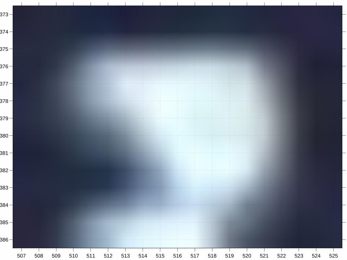
30/47What are we looking at?

507 508 509 510 511 512 513 514 515 516 517 518 519 520 521 522 523 524 525

373

374

375

376

377

378

379

380

381

382

383

384

385

386


31/47Did you recognize it?

100 200 300 400 500 600 700 800 900 1000

100

200

300

400

500

600

700


32/47Pixel images revisited

100 200 300 400 500 600 700 800 900 1000

100

200

300

400

500

600

700

59 110 161 212 263 314 365 416 467 518 569 620 671 722 773 824 875 926 977

119

170

221

272

323

507 508 509 510 511 512 513 514 515 516 517 518 519 520 521 522 523 524 525

373

374

375

376

377

378

379

380

381

382

383

384

385

386

� There are no negative coordinates. Where is the principal point?

� Lines are not lines any more.

� Pixels, considered independently, do not carry much information.


33/47Pixel coordinate system

Assume normalized geometricalcoordinates x = [x, y, 1]>

u = mu(−x) + u0

v = mvy + v0

where mu,mv are sizes of the pixelsand [u0, v0]> are coordinates of theprincipal point.

507 508 509 510 511 512 513 514 515 516 517 518 519 520 521 522 523 524 525

373

374

375

376

377

378

379

380

381

382

383

384

385

386

C

x

X

x

y

vu

[u0, v0]


34/47Put pixels and geometry together

From 3D to image coordinates:

λx

λy

λ

=

f 0 00 f 00 0 1

[ R t]X[4×1]

From normalized coordinates to pixels:

u

v

1

=

−mu 0 u0

0 mv v00 0 1

x

y

1

Put them together: 1λ

u

v

1

=

−fmu 0 u0

0 fmv v00 0 1

[ R t]X

Finally: u ' K[R t

]X

Introducing a 3× 4 camera projection matrix P: u ' PX


35/47Non-linear distortion

Several models exist. Less standardized than the linear model. We willconsider a simple on-parameter radial distortion. xn denote the linear imagecoordinates, xd the distorted ones.

xd = (1 + κr2)xn

where κ is the distortion parameter, and r2 = x2n + y2

n is the distance fromthe principal point.

Observable are the distorted pixel coordinates

ud = Kxd

Assume that we know κ. How to get the lines back?


36/47Undoing Radial Distortion

From pixels to distorted image coordinates: xd = K−1ud

From distorted to linear image coordinates: xn = xd1+κr2

Where is the problem? r2 = x2n + y2

n. We have unknowns on both sides ofthe equation.

Iterative solution:

1. initialize xn = xd

2. r2 = x2n + y2

n

3. compute xn = xd1+κr2

4. go to 2. (and repeat few times)

And back to pixels un = Kxn


37/47Undoing Radial Distortion

video


http://cmp.felk.cvut.cz/cmp/courses/XE33PVR/WS20072008/Lectures/../Videos/undoing_radial_dist.avi

38/47

Estimation of camera parameters—cameracalibration

The goal: estimate the 3× 4 camera projection matrix P and possibly theparameters of the non-linear distortion κ from images.

Assume a known projection [u, v]> of a 3D point X with known coordinates λu

λv

λ

=

P>1P>2P>3

X

Y

Z

1

λu

λ=

P>1 XP>3 X

andλv

λ=

P>2 XP>3 X

Re-arrange and assume6 λ 6= 0 to get set of homegeneous equations

uX>P3 −X>P1 = 0vX>P3 −X>P2 = 0

6see some notes about λ = 0 in the talk notes



39/47Estimation of the P matrix

uX>P3 −X>P1 = 0vX>P3 −X>P2 = 0

Re-shuffle into a matrix form:

[−X> 0> uX>

0> −X> vX>

]︸︷︷︸

A[2×12]

P1

P2

P3

︸︷︷︸p[12×1]

= 0[2×1]

A correspondece ui↔ Xi forms two homogeneous equations. P has 12parameters but scale does not matter. We need at least 6 2D ↔ 3D pairs toget a solution. We constitute A[≥12×12] data matrix and solve

p∗ = argmin‖Ap‖ subject to ‖p‖ = 1

which is a constrained LSQ problem. p∗ minimizes algebraic error


http://cmp.felk.cvut.cz/cmp/courses/XE33PVR/WS20072008/Lectures/Supporting/constrained_lsq.pdf

40/47

Decomposition of P into the calibrationparameters

P =[KR Kt

]and C = −R−1t

We know that R should be 3× 3 orthonormal, and K upper triangular.

P = P./norm(P(3,1:3));

[K,R] = rq(P(:,1:3));t = inv(K)*P(:,4);C = -R’*t;

See the slide notes for more details.



41/47An example of a calibration object

��

��

� �

� �

� �

��

��

��

� �

��

��

�

��

��


42/472D projections localized

0.43

0.72

0.92

0.55

0.50

0.33

0.65

0.82

0.63

0.40

5.65

3.17

4.31

0.39

0.56

0.53

0.22

4.99

0.47

2.73

0.78

0.34

0.22

0.46

0.14

2.28

2.64

5.44

4.50

0.35

0.79

2.65

0.54

0.43

0.21

0.45

0.82

0.56

0.13

0.30

2.79

2.35

2.59

3.82

4.78

0.62

0.46

0.36

0.36

0.27

2.21

6.19

2.77

2.62

3.96

6.43

5.98

2.70

2.29

7.74

4.37

2.76

2.44

2.85

2.85

2.84

3.85

2.54

2.59

6.27

505.79

5.27

3.57

3.43

6.32

4.52

2.73

2.85

2.10

6.36

2.97

3.41

2.17

6.56

503.36

2.21

8.23

502.59

2.10

503.14

2.19

5.05

8.55

2.75

2.95

8.39

503.38

4.64

6.21

2.08

1.78

3.99

4.66

2.56G

G

G

G

G

G

G

G

G

G

G

G

G

G

G

G

G

G

G

G

G

G

G

G

G

G

G

G

G

G

G

G

G

G

G

R

R

R

R

R

R

R

R

R

R

R

R

R

R

R

R

R

R

R

R

R

R

R

R

R

R

R

R

R

R

R

R

R

R

R

R

R

R

R

R

R

R

R

R

R

R

R

R

R

R

R

R

R

R

R

R

R

R

R

R

R

R

R

R

R

R

R

R

R

1

1

1

1

1

2

2

2

2

2

3

3

3

3

3

4

4

4

4

4

5

5

5

5

5

6

6

6

6

6

7

7

7

7

7

1

1

1

1

1

2

2

2

2

2

3

3

3

3

3

4

4

4

4

4

5

5

5

5

5

6

6

6

6

6

7

7

7

7

7

1

1

1

1

1

2

2

2

2

2

3

3

3

3

3

4

4

4

4

4

5

5

5

5

5

6

6

6

6

6

7

7

7

7

100 200 300 400 500 600

50

100

150

200

250

300

350

400

450


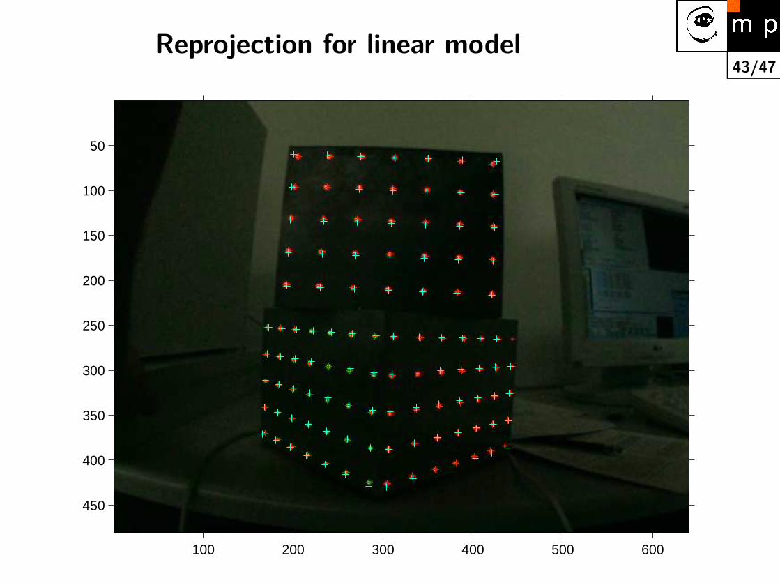
43/47Reprojection for linear model

100 200 300 400 500 600

50

100

150

200

250

300

350

400

450


44/47Reprojection for full model

100 200 300 400 500 600

50

100

150

200

250

300

350

400

450


45/47

Reprojection errors—comparison between full andlinear model

0 20 40 60 80 100 1200

1

2

3

4

5

6pi

xels

sorted 2D reprojection errors

full modellinear model


46/47References

The book [2] is the ultimate reference. It is a must read for anyone wantinguse cameras for 3D computing.

Details about matrix decompositions used throughout the lecture can befound at [1]

[1] Gene H. Golub and Charles F. Van Loan. Matrix Computation. JohnsHopkins Studies in the Mathematical Sciences. Johns Hopkins UniversityPress, Baltimore, USA, 3rd edition, 1996.

[2] Richard Hartley and Andrew Zisserman. Multiple view geometry incomputer vision. Cambridge University, Cambridge, 2nd edition, 2003.


47/47End


Z1

Z2

Z3

Z1

x

z optical axis

imag

epl

ane

imag

epl

ane

−f

X1

x1

C

x1−f = X1

Z1

x1 = −f X1Z1

Z1

Z2

Z3

Z1

Z2

x

z optical axis

imag

epl

ane

imag

epl

ane

−f

X1 X2

x1

x2C

X1 = X2x1 6= x2

Z2

Z3

Z2

Z3

x

z optical axis

imag

epl

ane

imag

epl

ane

−f

X2

X3

x2x3C

X2 6= X3x2 = x3

Z1

Z2

Z3

x

z optical axis

imag

epl

ane

imag

epl

ane

imag

epl

ane

imag

epl

ane

−f

f

X1 X2

X3

x1

x2x3

x1x2x3

C

X

X

X

X

X

X

X

X

X

X

x y

z

[0, 0, 0]

C

X

X

X

X

X

X

X

X

X

X

X

x y

z

[0, 0, 0]

C

x

X

X

X

X

X

X

X

X

X

X

X

x y

z

[0, 0, 0]

C

x

x y

z

[0, 0, 0]X

X

X

X

X

X

X

X

X

X

C

C

x

X

x y

z

[0, 0, 0]

C

x

X Xw

−Cw

Xcam

100 200 300 400 500 600 700 800 900 1000

100

200

300

400

500

600

700

59 110 161 212 263 314 365 416 467 518 569 620 671 722 773 824 875 926 977

119

170

221

272

323

100 200 300 400 500 600 700 800 900 1000

100

200

300

400

500

600

700

507 508 509 510 511 512 513 514 515 516 517 518 519 520 521 522 523 524 525

373

374

375

376

377

378

379

380

381

382

383

384

385

386

100 200 300 400 500 600 700 800 900 1000

100

200

300

400

500

600

700

59 110 161 212 263 314 365 416 467 518 569 620 671 722 773 824 875 926 977

119

170

221

272

323

507 508 509 510 511 512 513 514 515 516 517 518 519 520 521 522 523 524 525

373

374

375

376

377

378

379

380

381

382

383

384

385

386

C

x

X

x

y

vu

[u0, v0]

��

��

� �

� �

� �

��

��

��

� �

��

��

�

��

��

0.43

0.72

0.92

0.55

0.50

0.33

0.65

0.82

0.63

0.40

5.65

3.17

4.31

0.39

0.56

0.53

0.22

4.99

0.47

2.73

0.78

0.34

0.22

0.46

0.14

2.28

2.64

5.44

4.50

0.35

0.79

2.65

0.54

0.43

0.21

0.45

0.82

0.56

0.13

0.30

2.79

2.35

2.59

3.82

4.78

0.62

0.46

0.36

0.36

0.27

2.21

6.19

2.77

2.62

3.96

6.43

5.98

2.70

2.29

7.74

4.37

2.76

2.44

2.85

2.85

2.84

3.85

2.54

2.59

6.27

505.79

5.27

3.57

3.43

6.32

4.52

2.73

2.85

2.10

6.36

2.97

3.41

2.17

6.56

503.36

2.21

8.23

502.59

2.10

503.14

2.19

5.05

8.55

2.75

2.95

8.39

503.38

4.64

6.21

2.08

1.78

3.99

4.66

2.56G

G

G

G

G

G

G

G

G

G

G

G

G

G

G

G

G

G

G

G

G

G

G

G

G

G

G

G

G

G

G

G

G

G

G

R

R

R

R

R

R

R

R

R

R

R

R

R

R

R

R

R

R

R

R

R

R

R

R

R

R

R

R

R

R

R

R

R

R

R

R

R

R

R

R

R

R

R

R

R

R

R

R

R

R

R

R

R

R

R

R

R

R

R

R

R

R

R

R

R

R

R

R

R

1

1

1

1

1

2

2

2

2

2

3

3

3

3

3

4

4

4

4

4

5

5

5

5

5

6

6

6

6

6

7

7

7

7

7

1

1

1

1

1

2

2

2

2

2

3

3

3

3

3

4

4

4

4

4

5

5

5

5

5

6

6

6

6

6

7

7

7

7

7

1

1

1

1

1

2

2

2

2

2

3

3

3

3

3

4

4

4

4

4

5

5

5

5

5

6

6

6

6

6

7

7

7

7

100 200 300 400 500 600

50

100

150

200

250

300

350

400

450

100 200 300 400 500 600

50

100

150

200

250

300

350

400

450

0 20 40 60 80 100 1200

1

2

3

4

5

6pi

xels

sorted 2D reprojection errors

full modellinear model

geometryofimageformation - cmpcmp.felk.cvut.cz/cmp/courses/xe33pvr/ws20072008/lectures/...32/47...

Documents