CZECH TECHNICAL UNIVERSITY IN PRAGUE

Faculty of Mechanical Engineering

POLYTECHNIC UNIVERSITY OF VALENCIA CMT MOTORES TERMICOS

----------------------------------------------------------

MASTER THESIS

GEOMETRIC NOZZLE STUDY FOR AN EJECTION CYCLE USED FOR

WASTE HEAT RECOVERY IN AN INTERNAL COMBUSTION ENGINE

---------------------------------------------------

BY Deepak Kumar Jangid Gopalakrishnan

Supervisor Vit Doleček

Declaration of authorship

I hereby declare, that the master’s thesis I am submitting is entirely my original work except where

otherwise indicated. All the information derived from other works has been acknowledged in the

text and the list of references.

In Prague: 20.08.2018

------------------------------------------------

Deepak Kumar Jangid Gopalakrishnan

SUMMARY

In this thesis work, a detailed study is carried out on the operation of an integrated ejector

in a refrigeration cycle. The study has been done using mechanical simulation program of

computational fluid and aims to check the response of the different geometries of the ejector at

final operating conditions. The primary attention was given to the ejector geometry which

produces better performance, i.e., the geometry which minimizes the loss of pressure in the flow

and maximizes the ratio between the secondary and primary mass flow rate. After the ejector

geometry which produces optimum performance is found, the optimum geometry is studied in off-

design operating conditions to check if there is any reduction in the performance of the optimum

ejector geometry.

Throughout the project work, all the necessary steps are taken to configure and solve the

problem by using CFD simulation program. It is established as a starting point by setting up the

geometry followed by meshing process and mesh quality study. In the preprocessing, the attention

is given to the definition of the boundary conditions of the problem. The problem is initialized and

the simulated by using the resolution strategy. The process is concluded with the post-processing

phase and results of the analysis. The performance of optimum and non-optimum ejector

geometries is studied in detail with the flow behavior inside the ejector.

ACKNOWLEDGMENTS

I would like to express my sincere appreciation and gratitude to my supervisor Vicente Dolz

Ruiz from CMT Motores Termicos for his continuous support and guidance throughout my

internship and thesis study. Both his advice and assistance whenever necessary have been precious

in the development of my project. I wish to take the opportunity to thank the Polytechnic

University of Valencia and CMT Motores Termicos for accepting me to carry out internship and

thesis study.

I would also like to thank Alberto Ponce Mora who provided me an opportunity to work under

him as an intern and assisted me with his immense knowledge throughout the learning process of

my project.

Furthermore, I wish to thank Ing. Vit Doleček, Ph.D., my supervisor from Czech Technical

University for the guidance and input throughout my thesis work.

Most importantly I would like to thank my respected parents for having faith in my abilities and

constant support and encouragement throughout my studies Without their emotional and financial

support and their love the completion of this internship and thesis would not be possible.

In the end, I would like to display my appreciation to my partner and my beloved friends for their

significant role in my success.

Table of Contents

Chapter 1. INTRODUCTION ………………………………………………………………… 1

1.1. Project Background and Justification …………………………….…………… 1

1.2. Structure of the report …….………………………….…………………………. 2

1.3. Objective of my internship …………………………………………………….. 2

Chapter 2. THEORETICAL BASICS …………………………………………………………. 3

2.1. Ejection cycle ...………………………………………………………………. 3

2.1.1. Fundamental of the Refrigeration system by ejection cycle ......………... 3

2.1.2. Disadvantages of ejection cooling systems ..…………………………… 5

2.1.3. Ejector Classification ………………….……………………………………….. 5

2.1.4. Performance parameters of ejectors in the refrigeration cycle ………………… 8

2.1.5. Ejector operation ................................................................................................. 9

2.1.6. Working fluid ..................................................................................................... 11

2.1.7. Integration in an Internal Combustion Engine ...……………………………… 12

2.2. Convergent- Divergent Nozzle ...…..………………………………………………… 14

2.2.1. Flow Regimes in a Convergent-Divergent Nozzle ...…………………………. 15

2.3. Objective of my internship …………………………………………………………... 17

Chapter 3. CFD MODEL ….…………………………………………………………..…… 18

3.1. Introduction ..…….…………………………………………………………. 18

3.1.1. Preprocessing …………………………………………………………. 18

3.1.2. Simulation …….………………………………………………………. 19

3.1.3. Postprocessing ….……………………………………………………... 19

3.2. Ejector Modeling …………………………………………………………….. 20

3.2.1. Geometric design of ejector ................................................................... 20

3.2.2. Mesh generation ……………………………………………….. 22

3.2.3. Configuration of the case ……………………………………… 25

3.2.3.1. General configuration ………………………………… 25

3.2.3.2. Turbulence Model ……………………………………. 25

3.2.3.3. Fluid Material ………………………………………… 26

3.2.3.4. Boundary Conditions ………………………………… 26

3.2.3.5. Solution Method and Relaxation Factor ..……………. 27

3.2.4. Resolution …………………………………………………….. 28

3.2.4.1. Quasi-stationary start of the ejector ...……………….. 28

3.2.4.2. Stability of the calculation and convergence criteria ... 28

Chapter 4. CONVERGENT-DIVERGENT EJECTOR OPTIMIZATION STUDY ………. 30

4.1. Convergent-Divergent ejector geometry optimization results …………….. 31

4.1.1. Optimum ejector geometry ………………………………………… 31

4.1.2. Non-optimum ejector geometries ………………………………….. 35

4.1.3. Negative entrainment ratio ………………………………………… 39

Chapter 5. STUDY OF OPTIMUM EJECTOR OPERATION IN OFF-DESIGN

CONDITIONS …………………………………………………………………. 40

5.1. Off-design operating conditions and simplified ejector models …………... 41

Chapter 6. CONCLUSION ………………………………………………………………… 46

Chapter 7. ANNEX ………………………………………………………………………… 47

REFERENCES ………………………………………………………………………………. 52

List of Figures

Figure 2.1. Schematic representation of the ejection cooling cycle …………………………… 4

Figure 2.2. Supersonic ejector operating mode (a) fixed primary pressure, and (b) fixed back

Pressure ……………………….…………………………………………………… 9

Figure 2.3. Typical ejector operating curve ………………………………………………….. 11

Figure 2.4. Different operating regimes of convergent-divergent nozzle ……………………. 15

Figure 3.1. Geometry of ejector designed in the previous project …………………………… 20

Figure 3.2. Detailed view of changed convergent-divergent ejector with important

dimensions ……………………………………………………………………….. 21

Figure 3.3. Divided segments for meshing. a) general view of convergent-divergent ejector

b) detailed view of convergent-divergent ejector ……………………………….. 23

Figure 3.4. Detail view of the mesh of convergent-divergent ejector nozzle ………………... 2

Figure 3.5. Definition of boundary conditions of an ejector according to the following color

codes. Black – wall, red – pressure inlet, purple – pressure outlet,

light green – axis symmetric …………………………………………………….. 26

Figure 4.1. Dimensions of ejector geometry whose influence has been studied. (d2) nozzle exit

diameter and (d4) mixing chamber diameter …………………………………… 31

Figure 4.2. Optimum geometry of convergent-divergent ejector …………………………… 32

Figure 4.3. Stabilization of secondary mass flow rate ……………………………………….. 32

Figure 4.4. Mach contour of optimum convergent-divergent ejector geometry …………….. 34

Figure 4.5. Pressure contour of optimum convergent-divergent ejector geometry …………. 34

Figure 4.6. Mach contours over different mixing chamber diameter with constant nozzle exit

diameter D = 2.2 mm. (A) D = 3.2 mm, (B) D = 3.6 mm, (C) D = 2.8 mm ……. 36

Figure 4.7. Mach contours over different nozzle exit diameter with constant mixing chamber

diameter D = 3.2 mm. (D) D = 2.2 mm, (E) D = 2.4 mm, (F) D = 1.6 mm …….. 38

Figure 4.8. Mach contour of ejector geometry ( nozzle exit diameter = 3.2 mm and mixing

chamber diameter = 4.4 mm) with negative entrainment ratio …………………. 39

Figure 5.1. Jet ejector characteristic surfaces ………………………………………………. 40

Figure 5.2. Off-design pressure results with corresponding fitted critical and sub critical

Surfaces ………………………………………………………………………… 42

Figure 5.3. Mach number contours over different backpressure with fixes primary inlet

Pressure Pp = 40 bar, and secondary inlet flow pressure Ps = 5.5 bar. (G) Po = 10

bar, (H) Po = 12 bar, (I) Po = 14 bar ..………………………………………… 45

List of Tables

Table 2.1. Ejector classification ………………………………………………………………... 7

Table 3.1. Numerical dimensions of the changed convergent-divergent ejector ……………... 22

Table 3.2. Numerical values of the parameters of quality check for mesh …………………… 24

Table 3.3. Model Constants of SST k-ꞷ ……………………………………………………… 25

Table 3.4. Properties of Air …………………………………………………………………… 26

Table 3.5. Relaxation Factors for coupled and simple scheme ………………………………………………… 27

Table 4.1. Final boundary conditions for the study of ejector optimization ………….………. 30

Table 4.2. Optimum Values of Ejector Geometry …………………………………….……… 32

Table 4.3. Reduction of entrainment ratio of the ejector geometry of case (B) and (C) from

optimum case ……………………………….…………………………………………………………………………. 35

Table 4.4. Reduction of entrainment ratio of the ejector geometry of case (E) and (F) from

optimum case …………………………………………………………………….. 37

Table 5.1. Fitting coefficients for critical and subcritical characteristic surfaces …………… 42

Table 5.2. Maximum relative error between simulated points and the fitting surfaces for critical

and subcritical surfaces ………………………………………………………….. 44

Table A.1. Change of pressure conditions and number of iterations required to solve

The case ………………………………………………………………………… 47

Table A.2. Summary of the results obtained for different geometrical designs of convergent-

divergent ejector and final boundary conditions 40 bar (primary inlet pressure),

5 bar (secondary inlet pressure) and 13 bar (outlet pressure) …………………. 48

Table A.3. Summary of the results obtained for different geometrical designs of convergent-

divergent ejector and final boundary conditions 40 bar (primary inlet pressure),

5 bar (secondary inlet pressure) and 13 bar (outlet pressure) …………………. 49

Table A.4. Summary of the results obtained for off-design operating pressures of optimum

convergent-divergent ejector ……………………………………………………… 50

Table A.5. Summary of the results obtained for off-design operating pressures of optimum

convergent-divergent ejector ……………………………………………………… 51

Index of Terminology

(𝑹𝒄)

Compression ratio

(CC)

Cooling Capacity

(COP)

The coefficient of performance

𝛽 Curve fit coefficient

(ηejector)

Efficiency of ejector

(𝝎)

Entrainment ratio

crit Ejector critical operational mode

Scrit Ejector subcritical operational mode

I-VI Generic index

��

Mass flow rate (kg/s)

( π0p)

Outlet-primary pressure ratio

( πsp)

Secondary-primary pressure ratio

1

Chapter 1. INTRODUCTION

1.1 Project Background and Justification.

This thesis is carried out with the collaboration of CMT Motores Termicos and Czech

Technical University. CMT Motores Termicos is a research and educational institute a part of the

polytechnic university of Valencia which is fully involved in the development of the future

combustion engine. Its studies mainly involve at investigating thermal processes and fluid

dynamics of alternative internal combustion engines. Many of these projects have taken place in

collaboration with prestigious companies linked directly or indirectly with the alternative internal

combustion engines: Renault, PSA Group (Peugeot-Citroen), Nissan, Volvo, Ford, BMW, Bosch,

ECIA, Iveco, MAN, Repsol, General Motors, RENFE or the EMT of Valencia. They also carry

out research in combustion, air management, thermal management, noise control, CFD. One of the

researches includes the use of residual thermal energy in the ejection cycle for cooling the intake

air. This project is a part of the research on the recovery system.

In an internal combustion engine, two third of the fuel energy is rejected to the environment

by means of the refrigeration system and exhaust gases. The gases derived from the exhaust system

have residual thermal energy and could be exploited. In the past, many efforts were made to try to

take advantage of the energy available to the maximum. For example, Japanese company DENSO

has developed the first practical concept of air conditioning system that uses ejection cycle

technology which reduces compressor workload and improving fuel economy [1].

In the past, many researchers have focused on improvement of ejection cycles which has lower

impact on the environment and which supports a more efficient use of available resources. The

results show that the ejection cycle seems to be a efficient way of taking advantage of low-grade

waste heat produced from vehicle exhaust. However, it has been seen poor performance of ejector

nozzle when operating in off design conditions. Due to lower COP values in comparison with other

technologies like traditional air-compressing cooling system along with poor performance of

ejector in off design operating condition are the reasons for limited market penetration till date.

CMT is conducting research on the optimization of the ejector in operating conditions and

integrating the ejection cycle in an automotive engine with a working fluid R134a which is usually

used in a refrigeration system and to check the ejector performance when working in off-design

operating conditions because in an internal combustion engine of a vehicle, it is usual to work in

different operating mode. Therefore, my thesis will be focusing on the same optimization of an

ejector with a different working fluid, and it will be explained in detail in this thesis. Air as a

working fluid is chosen for this project because it was one of the requirements by CMT for their

future practical application. Optimization of ejector nozzle geometry has been carried out in CFD

2

software. The performance of ejector in off-design operating conditions has been evaluated by

means of characteristic surfaces which represents operating pressures against ejector entrainment

ratio. This method is unique to each geometry and has been often used by some authors [9] [10].

1.2. Structure of The Report

The report structure is divided into following chapters:

• Chapter 2 describes the theoretical basics of the ejection cycle along with the essential

functions of ejector components and performance parameters.

• Chapter 3 CFD model explains the entire simulation process in detail. starting with

Preprocessing where geometry is defined following the meshing phase and setting up the

model for calculation and then simulation and postprocessing.

• Chapter 4 describes the results in detail obtained from the simulation for the optimum and

non-optimum ejector geometry.

• Chapter 5 contains the study of optimum ejector operation in off-design operating

conditions.

• Chapter 6 gives the conclusion from the results obtained.

• Chapter 7 Annex: In this part, all the tables containing the data obtained from simulation.

1.3. Objective of My Internship

To do a literature study on the ejection cycle and ejector design and obtain knowledge on

the working principle of ejection cycle and convergent-divergent ejector.

Also, to study the relationship between the different operating pressures and the conditions

of the flow in the ejector, i.e., the existence of shock waves, the evolution of mixing process,

blocking and recirculation of the flow in the secondary chamber.

The main objective of my internship is to design an ejector geometry and optimize the

ejector geometry with a working fluid as air as an ideal gas model in specific operating conditions

of an automotive engine in terms of exhaust energy available and required cooling capacities and

to check the behavior of optimum ejector geometry in off-design conditions.

3

.

Chapter 2. THEORETICAL BASICS

2.1. Ejection Cycle

2.1.1. Fundamental of the Refrigeration system by ejection cycle

The increasing demand for thermal comfort has led to a rapid increase in the use of the

refrigeration system and, consequently, in energy consumption. The development of thermal

refrigeration system using low-grade heat or solar energy would provide a significant reduction of

energy consumption and has a promising future in many applications [2].

The use of thermal refrigeration system for cooling is based on the operation of

consumption of energy in the form of residual heat from industrial processes or chemical industries

and among the various technologies for a thermal refrigeration system, heat-driven ejector

refrigeration system seems like an exciting alternative to the traditional compressor-based

technologies. In the present state of development, the thermal refrigeration system produces lower

COP (Coefficient of performance), defined as the ratio between the cooling effect and the heat

input to the generator, than the compressed-based system. They have various advantages like

reliability, limited maintenance needs and low initial and operational costs [2]. Due to this reason,

the thermal refrigeration system has resulted fascinating for a high number of applications with

different refrigerant capacity requirements (from few kW to 60,000 kW).

Figure 2.1 in the below represents the basic configuration of the ejection cooling cycle

which consists of various elements like generator, condenser, evaporator, pump, expansion valve

and an ejector. The below configuration is divided into two loops, the power loop, and the cooling

loop.

4

6

5 4

2

3

Pump

1

Wp

Qg

Qc

Qe

Figure 2.1: Schematic representation of the ejection cooling cycle.

In the power loop, the thermal energy from the heat source is used to evaporate the working

fluid (refrigerant) at high pressure and temperature in a generator (a process that takes place

between the point 1 and 2). The resulting steam at high pressure constitutes the primary stream or

the mainstream of the ejector which flows and inside of the ejector it expands and accelerates at

supersonic speed. The ejector consists of a section of secondary entrance for the secondary fluid

at low pressure downstream of the nozzle from the evaporator and a mainstream entrance for the

primary fluid at high pressure upstream of the ejector. As the primary stream enters the mixing

chamber, the primary flow entrains the secondary fluid coming from the evaporator at point 3. The

mixing process of two streams takes place, and the kinetic energy from the primary current is

transferred to the secondary flow. Subsequently, the mixed stream enters the subsonic diffuser area

where there is a partial recovery of pressure and the flow decelerates. After that, the combined

Generator

Evaporator

0

Condenser EJECTOR

Expansion

valve

5

stream exits the ejector and enters the condenser at point 4. Inside the condenser, the phase change

takes place where it changes to liquid phase yielding heat to the cold environment. After this

condensation process, the condensate split into two currents: one is expanded through an expansion

valve and fed back to the evaporator which completes the cooling loop, or the refrigeration loop

and the other flow is recirculated to the generator by a pump to complete the power loop [3]. In

the refrigeration loop, when the element to be cooled is found at a higher temperature than the

working fluid, there is a transfer of heat from the component to be cooled to the working fluid. At

point 3, the vapor phase from the evaporator outlet carried back to the secondary inlet of the

ejector.

2.1.2. Disadvantages of ejection cooling systems

In comparison with other refrigeration methods the ejection cooling system is not used at

the industrial level due to the following reasons:

• Low COP (Co-efficient of Performance) values less than 0.2 when compared to

compression systems even neglecting the energy required by the pump to function.

• The value of the COP drops significantly when working in off-design conditions, i.e., when

working outside the design point.

• The central aspect that hinders its implementation in any sectors is due to the lack of

experimental and theoretical data on their performance in the different application.

2.1.3 Ejector Classification

An ejector can be classified by (i) the nozzle position, (ii) nozzle design and (iii) the

number of phases, as outlined in Table 2.1. In the following paragraphs, these classifications are

detailed.

Based on the nozzle position, there are two general configurations and one in experimental phase

which was proposed by Eames [2].

6

• CPM ejector (Constant-pressure mixing ejector): In CPM ejector, the nozzle exit is in

the suction chamber, and the mixing process takes place in the suction chamber. They

widely use CPM ejector because of their ability to operate against larger backpressures.

• CAM ejector (Constant-area mixing ejector): In CAM ejector, the nozzle exit is placed

in the constant-area section, and the mixing process takes place in the constant area section.

CPM ejectors are better in performance than the CAM ejectors although CAM ejectors can

produce higher mass flow rates.

• CRMC ejector (Constant rate of momentum-change ejector): This ejector seeks to

combine the best aspects of CPM and CAM ejectors. The CRMC configuration uses a

variable area section rather a constant area section, which provides an optimum flow

passage area to reduce the thermodynamic shock thus increasing ejector performance. The

method assumes a constant rate of change of momentum within the duct.

One of the parameters which affect the ejector operation is the nozzle design. Based on the

nozzle shape they are categorized into two regimes:

• Ejector with the subsonic regime: The nozzle shape is convergent, i.e., the ejector works

in a subsonic system, and it can reach sonic condition at the suction exit. Subsonic ejectors

are not designed to produce a significant fluid compression, but they must provide little

pressure loss. They can employ in industrial plants for Chemical looping combustion

(CLC) power plants and transcritical CO2 ejector refrigeration system (TERS) [2].

• Ejector with the supersonic regime: In this type, the nozzle shape is convergent-

divergent and reaches supersonic condition at the nozzle exit. Supersonic ejectors are used

when there is a need to generate a high-pressure difference. In the supersonic regime, the

primary flow can entrain a high quantity of suction fluid because of the lower-pressure at

the nozzle exit and high momentum transfer. Their primary applications are fuel cell

recirculation system, i.e., molten carbonate fuel cells and solid oxide fuel cells [2].

The last classification of the ejectors is based on the number of phases. Depending on the

primary and secondary flow conditions, the flow inside the ejector can be either single phase (gas-

gas or liquid-liquid) or two phases (liquid-gas). The nature of the two-phase flow may classify a

two-phase ejector: (i) a condensing ejector (the primary flow condensates in the ejector) and (ii) a

two-phase ejector (where the stream at the outlet is two-phase). At present, the modeling of the

two-phase ejector is still limited due to their enormous complexity.

7

Rem

ark

s

Bet

ter

per

form

ance

th

an C

AM

ejec

tor

- - -

Po

ssib

le t

wo

-ph

ase

flo

w a

nd

sho

ck w

aves

No

sh

ock

wav

es, si

ng

le-p

has

e

flo

w o

nly

Tw

o-p

has

e fl

ow

wit

h p

rim

ary

flo

w c

on

den

sati

on

an

d s

tro

ng

sho

ck w

aves

Tw

o-p

has

e fl

ow

an

d p

oss

ible

sho

ck w

aves

Cla

ssif

ica

tio

n

CP

M e

ject

or

CA

M e

ject

or

Su

bso

nic

eje

cto

r

Su

per

son

ic e

ject

or

Vap

or

jet

ejec

tor

Liq

uid

jet

eje

cto

r

Co

nd

ensi

ng

eje

cto

r

Tw

o-p

has

e ej

ecto

r

Co

nd

itio

n

Insi

de

suct

ion

ch

amb

er

Insi

de

con

stan

t-ar

ea s

ecti

on

Co

nv

erg

ent

Co

nv

erg

ent-

Div

erg

ent

Ex

it f

low

Vap

or

Liq

uid

Liq

uid

Tw

o-

ph

ase

Seco

nd

ary

flo

w

Vap

or

Liq

uid

Liq

uid

Vap

or

Prim

ary

flo

w

Vap

or

Liq

uid

Vap

or

Liq

uid

Pa

ra

mete

rs

No

zzle

po

siti

on

No

zzle

desi

gn

Nu

mb

er o

f

ph

ase

s

Tab

le 2

.1. E

ject

or

class

ific

atio

n [

2]

8

2.1.4. Performance parameters of ejectors in the refrigeration cycle

The performance of ejectors and its cooling capacity of the system can be quantified based on

several parameters which are used to characterize ejectors:

• Entrainment ratio (𝝎): It is defined as the ratio between the mass flow rate of secondary

flow (��s) and the mass flow rate of the primary flow (��p). The entrainment ratio evaluates

the efficiency of the cooling cycle. Equation (2.1) represents the mathematic expression.

𝝎 =��𝒔

��𝒑 (2.1)

• Compression ratio (𝑹𝒄): It is defined as the ratio between the static pressure at the exit of

the diffuser (Pc) and the static pressure of the secondary flow (Pe). Equation (2.2) represents

the mathematic expression.

𝑹𝒄 =𝑷𝒄

𝑷𝒆 (2.2)

• The coefficient of performance (COP): It is defined as the ratio between evaporation heat

energy, Qe (cooling effect), and the total incoming energy into the cycle (Qg + Wp).

Equation 2.3 represents the mathematic expression.

𝑪𝑶𝑷 =𝑸𝒆

𝑸𝒈+ 𝑾𝒑 (2.3)

Where Qg refers to the energy contributed to the generator, and Wp refers to the

mechanical work required by the pump to circulate the fluid.

• Cooling Capacity (CC): It is defined as the product of a secondary mass flow rate and

the specific enthalpy difference at the evaporator. Equation (2.4) represents the

mathematic expression.

𝑪𝑪 = ��𝒆 ∙ (𝒉𝒆,𝒐𝒖𝒕 − 𝒉𝒆,𝒊𝒏) (2.4)

• Ejector efficiency (ηejector): It is defined as the ratio between the actual recovered

compression energy and the available theoretical energy in the motive stream. Equation

(2.5) represents the mathematic expression.

ηejector = (��𝒈+��𝒆) ∙ (𝒉𝒄,𝒊𝒏−𝒉𝒆,𝒐𝒖𝒕)

��𝒈 ∙ (𝒉𝒈,𝒐𝒖𝒕−𝒉𝒆,𝒐𝒖𝒕) (2.5)

Where ��𝑔 and ��𝑒 refers to the mass flow rate of the primary and secondary flow

respectively. In addition, ℎ𝑔 represents specific enthalpy of the primary flow and ℎ𝑐

represents the specific enthalpy of the condenser.

9

2.1.5. Ejector Operation

For improving the efficiency of the energy recovery system, nozzle geometry plays the most

critical part. Based on the geometry, the ejector can be subsonic or supersonic ejector, and this is

taken as a general design criterion. Based on the results obtained experimentally inside the ejector,

nozzle type and nozzle geometry are the most critical design parameters. The nozzle shape can be

convergent if the ejector operates under subsonic conditions at the suction exit or it can be

convergent-divergent if the ejector operates under supersonic conditions at the suction exit.

Subsonic ejectors are not designed to produce a high variation of pressure in the fluid, but they can

minimize pressure losses. On the other hand, supersonic ejectors are the right option when working

with a high-pressure difference at the entry and exit of the nozzle. Also, in the supersonic regime,

they facilitate the mixing process of the primary and secondary stream because of the high

momentum transfer. Another significant effect is that the primary flow can entrain a high quantity

of the secondary flow due to the low pressure at the nozzle exit [2].

Both subsonic and supersonic ejector works in the different operating regimes. Since the study

in this project is carried out only on a supersonic ejector, three different operating modes of the

supersonic ejector are shown in figure 2.2.

Figure 2.2: Supersonic ejector operating mode (a) fixed primary pressure, and (b) fixed back

pressure

The Supersonic ejector can work in three different operating modes such as critical mode, sub-

critical mode, and backflow as shown in figure 2.2 above.

10

• Critical mode (double-choking): In the critical mode, the entrainment ratio remains

constant because the primary and secondary flows are choked. Choking phenomenon is an

important phenomenon which is related to secondary flow. Due to this choking

phenomenon in the critical mode, it limits the maximum flow rate through the ejector, and

thus the cooling capacity (CC) and the coefficient of performance (COP) remains constant.

More specifically, the expansion waves of primary fluid due to under-expansion create a

converging duct where there is no mixing. In this situation, the secondary flow feels the

decrease of the useful cross section reaching supersonic speeds and chokes in a specific

position that depends on the operating conditions. Therefore, the secondary current is not

affected by the back pressure and can increase with primary pressure only.

• Sub-critical mode (single-choking): In the sub-critical mode, the primary flow is choked,

and the entrainment ratio varies linearly with the increase in back pressure at the outlet of

the ejector. During subcritical mode value of backpressure influences ejector operation. In

this case, when the value of back pressure increases, a shock wave is displaced into the

mixing chamber interacting with the mixing [2]. A further increase in backpressure leads

to further movement of shockwave into the mixing chamber and reversing the primary flow

into the suction chamber. The pressure value of the discharge which separates the critical

and subcritical mode is called critical pressure [3].

• Backflow (malfunction mode): In this mode, the flow coming from an outlet or the

primary flow penetrates the secondary chamber because of the pressure at the primary

chamber entrance and the back pressure at the outlet are very high. This phenomenon

causes the ejector to malfunction. It is also possible that this operating principle takes place

when the pressure in the secondary chamber is very low.

A change in evaporator and generator conditions leads to substantial changes in the entrainment

ratio and critical pressure [3]. Figure 2.3 shows the typical operating curve. When the evaporator

temperature increases as in figure 2.3, the entrainment ratio increases as a result of the higher

secondary mass flux. Also, the higher temperature of saturation in the evaporator leads to higher

critical pressures (due to the higher total pressure of the suction flow. Changing the focus, when

the pressure increases in the generator as in Figure 2.3, the primary flow is increased, but higher

entrainment ratio is not obtained because the secondary flow remains constant. Consequently, the

entrainment ratio decreases. However, in this scenario it will be admissible to increase the back

pressure, thus increasing the critical pressure.

11

Figure 2.3. Typical ejector operating curve [2].

As it is seen that the operating point of the ejector will be given by the conditions of pressure and

the temperature in the primary and secondary chamber in addition to the output.

2.1.6. Working Fluid

The selection of the appropriate working fluid has high relevance to the design of an ejector

refrigeration system. Traditionally the primary criteria at the time of selecting the working fluid

have been to maximize the performance. Other factors like safety, cost, etc., are also considered,

but the final choice depends on the compromise between the performance and the environmental

impact. In this regard, we may pay attention to the ODP (Ozone Depletion Potential) and the GWP

(Global Warming Potential). In general, the suitable coolant for a cooling system must be chosen

in such a way that high performance is guaranteed for the operating conditions of the ejector.

Accordingly, the thermal properties of the coolant should be considered. There are specific

constraints which should be satisfied by the thermal properties of the refrigerant such as large

latent heat of vaporization or critical temperature relatively high used to compensate for significant

variations in generator temperatures. Also, the fluid pressure in the generator should not be too

high for the design of the pressure vessel and to limit the pump energy consumption. Moreover,

the viscosity, the thermal conductivity and the other properties that influence the heat transfer

should be as favorable as possible. A high molecular mass also contributes to maximizing the

entrainment ratio and ejector efficiency. However, this requires smaller ejectors, thus introducing

difficulties in the design and behavior due to the smaller size of the components [2].

12

Other desirable qualities of the working fluid are a low environmental impact, low cost, non-

explosive, non-toxic, non-corrosive, chemical stability, and availability in the market. For

example, Water as a working fluid provides excellent performance as it has a high heat of

vaporization, has a reduced cost and the environmental impact is very low. However, the working

temperature must be above 0 oC, which limits the maximum achievable COP (Coefficient of

Performance). Also, a T-s diagram of water does not favor its implementation in ejection cycles

compared to others, and because of its high specific volume, large diameter pipes are required to

minimize the pressure losses. Therefore, water is rarely used in real life cooling system but often

employed in experimental devices. In practical applications other coolants are used which are

chemical compounds, the most common chemical compound is halocarbons and organic

compounds formed by hydrogen and carbon.

2.1.7. Integration in an Internal Combustion Engine

Ejection cycle shows a lot of potential benefits when integrated within the internal

combustion engine. It raises air conditioning performance and reduces air intake temperature.

Japanese company DENSO developed the first practical concept and implemented in a vehicle as

a substitute for the expansion valve in a conventional air conditioning cycle. Several designs using

different approaches with jet ejector technology have been patented by DENSO. One of the

developments in ejector technology has been applied in passenger car vehicles, specifically in

Toyota Prius and it reduced power consumption of compressor in a conventional air-conditioning

system by up to 25%, hence reducing compressor workload and improving fuel economy [1].

In the last few years, many efforts have been carried out in need of vehicles with a lower

environmental impact which has led to an increase in these technologies. One of the approaches is

“Heat to cool” which is associated with different strategies of waste heat recovery which focuses

on developing useful forms of recovery of energy, mainly by taking advantage of the energy

contained in the exhaust gases in the engine offers excellent possibilities. Because in an internal

combustion engine (ICE) only one-third of the fuel energy available is transformed into

mechanical energy. The remaining two-thirds is rejected to the environment by means of the

refrigeration system and as exhaust gas waste heat. As a heat source, it has been shown that the

gases rejected by the exhaust system offer more possibilities than the coolant system because of

its higher temperature level despite its increased engine back pressure due to the exhaust gas

exchanger.

13

This ejector technology is integrated with an internal combustion engine to generate

cooling capacity by means of a waste exhaust gas driven ejector cooling system in order to reduce

the intake air temperature which in turn increases engine efficiency. For a given engine operation

point, the effective efficiency of the engine (𝜂eff) depend on the charge air density (ρ). According

to the equation of ideal gas (equation 2.6), an increase of the air density (ρ) can be achieved either

by an increasing the pressure or by decreasing the temperature of charge air.

𝜌 =𝑃

(𝑅∙𝑇) (2.6)

At present, turbocharging is the established technology which is used to take advantage of

the exhaust gas energy by compressing the charge air above the ambient pressure particularly for

diesel engines. The result is increased effective engine power and effective engine efficiency.

During non-isothermal compression, the charge air temperature increases due to which thermal

load in the turbocharger turbine also increases . In gasoline engines, an increased charge air

temperature might lead to uncontrolled combustion which is called as knocking. To avoid this

problem, intercoolers are used to cool the gases at the compressor outlet.

By incorporating ejector technologies in the internal combustion engine in order to reduce

intake air temperature by means of a waste heat recovery system lot of both direct and indirect

benefits are obtained. One of the direct positive effects is seen as the improvement in volumetric

efficiency which is directly related to the reduction of intake air. However, many of potential

advantages are not directly related to this phenomenon. Below are the listed potential advantages

due to the reduction of intake air.

• A reduction of intake air temperature allows advancement of ignition timing due to lower

knocking tendency. An efficiency increases of more than 13% was achieved due to

ignition advancement only [4].

• Peak combustion temperatures are reduced during combustion which leads to a reduction

of NOx emissions due to the reduced intake air temperature.

• Thermal loads are also reduced by the reduction of intake air temperature which in turn

contributes engine with higher indicated efficiency.

• Uncontrolled combustion phenomenon is known as knocking prevented in turbocharged

gasoline engines.

14

• Improved performance near surge conditions by reducing intake air temperature.

• Lower combustion temperatures which are associated to charge air cooling means lower

turbine inlet temperatures which result in reduced thermal stresses.

• In turbocharged engines, air cooling is beneficial because it helps to avoid compressor

pumping.

2.2. Convergent Divergent Nozzle

Nozzles are used to modify the flow of a fluid. It is done by increasing the kinetic energy of

the stream in the expense of its pressure. Convergent-divergent nozzles are mostly used for

supersonic flows. In convergent nozzle, it is impossible to create supersonic flows (M > 1), and

therefore it restricts us to a limited amount of mass flow through a nozzle. In convergent-divergent

nozzle, we can increase the stream velocity more than sonic velocity. Due to this reason, they have

important applications such as propelling nozzle in jet engines or in air intake system for internal

combustion engines working at higher rpms.

To understand the one-dimensional flow process in a convergent-divergent nozzle we have to

treat magnitudes of the fluid such as density (ρ), cross-section area (A), velocity and mass as

constant. The flow is isentropic if the adiabatic conditions are attained (i.e., entropy is uniform).

After all the assumptions we reach to equation (2.7) [5]. Equation 2.7 is for an isentropic process

and for an ideal gas.

𝑑𝐴

𝐴=

𝑑𝑢

𝑢(𝑀2 − 1) (2.7)

From equation (2.7), the following important conclusion is drawn.

• For subsonic velocities (M < 1), dA and du must be opposite in sign. Therefore, increase

in the area of cross-section (𝑑𝐴

𝐴> 0) causes a decrease in velocity (

𝑑𝑢

𝑢< 0) and vice versa.

• For supersonic velocities (M > 1), dA and du are of the same sign. Therefore, the increase

in the area of cross section causes an increase in velocity and decrease in the area of cross

section causes a decrease in velocity.

15

2.2.1. Flow Regimes in A Convergent-Divergent Nozzle

For this case study, the flow in the nozzle is intended to accelerate from subsonic velocity

to supersonic velocity. Therefore, it is necessary to use a convergent-divergent nozzle. In the

convergent part, the area of cross-section reduces gradually in the flow direction. The flow in the

convergent nozzle is still subsonic and the mass flow rate and flow velocity increases till it reaches

Mach number (M=1), i.e., sonic condition. After that, the flow reaches sonic conditions, and the

flow is choked whatever the backpressure value. There is no supersonic region in the convergent

nozzle whatever the backpressure value. At the divergent nozzle, the principle reverses, and the

flow speed increases with the decrease in back pressure and the mass flow rate. Therefore, it

reaches supersonic conditions (M > 1). The convergent-divergent nozzle has different operating

regimes depending on the back pressure values as shown in figure (2.4).

Figure 2.4. Different operating regimes of the convergent-divergent nozzle [5].

16

• Back pressures (p1 and p2): The back-pressure values of p1 and p2 are above the value

corresponding to M=1 at the nozzle throat. In this regime, the static pressure first decreases

along the chamber and then increases, with a corresponding increase and decrease in

velocity. The flow in this regime is subsonic.

• Back pressure (p3): When the back pressure is decreased to p3, the Mach number reaches

unity at the nozzle throat. The flow at the upstream of the nozzle is subsonic, reaches sonic

at M = 1 and then subsonic at the downstream of the nozzle .

• Back pressure (p8) : When the back-pressure value is p8, the flow at the upstream of the

nozzle is subsonic and reaches sonic at M = 1. But at the downstream of the nozzle, the

flow reaches supersonic regime.

The above-mentioned regimes of convergent-divergent nozzle for different back pressures are

the only possibilities of isentropic, one-dimensional steady flow. To describe the other levels of

back pressure, the isentropic constraint must be relaxed.

• Back pressure (between p3 and p8): In this range of back pressure values between p3 and

p8 the pressure and the velocity in the nozzle are discontinuous. Between p3 and p5 There

is a region of supersonic flow downstream of the nozzle, followed by a normal shock and

then a region of subsonic flow. The condition of the strength of the shock is when the exit

flow is subsonic, the exit pressure is equal to the back pressure. The strength of the shock

increases when the back pressure value is lowered.

At a back pressure value of p5, the normal shock occurs at the nozzle exit and the

flow in the region between throat and nozzle exit is supersonic. No further changes can

occur as the pressure is lowered from this point.

The behavior of the flow between the nozzle exit and the downstream for the back

pressure values between p5 and p8 does not takes place in one-dimensional manner but

instead occurs in a series of oblique shock waves as sketched in figure 2.4. The flow

between the back pressure values of p5 and p8 is known as overexpanded.

Decreasing the back pressure beyond p8 means the flow at the exit is at a higher

pressure than the surroundings. Adjustment to a final state with a pressure equal to the back

pressure then occurs through a series of expansion waves. For back pressures lower than

p8, the flow is said to be underexpanded [5].

17

18

Chapter 3. CFD Model

3.1. Introduction

In this chapter, all the steps of CFD modeling will be discussed briefly in sequential order,

Preprocessing, simulation and post-processing is done using software ANSYS FLUENT.

Explanation of geometry of ejector prototype using ANSYS CAD tool and justification of all the

decisions made in reference to meshing, turbulence model, and boundary conditions. Also, the

convergence of the calculation is ensured while solving the case.

Computational fluid dynamics (CFD) is a branch of fluid mechanics which solves problems

involving fluid flows by means of numerical analysis and data structures. The use of computers

solves millions of calculations required to simulate the interactions of liquid and gases with the

surfaces defined by boundary conditions. The algorithm implemented in the CFD setup allows

solving equations iteratively simplified in the volume space discretized by a mesh. Despite the use

of complex equations and large iterations, the results obtained are only approximate in some cases.

Below we will discuss the fundamental procedure which is always followed in CFD setup

(Preprocessing, simulation and post-processing).

3.1.1. Preprocessing

The central principle of preprocessing is to model the case to be solved in a definite way

so that the CFD program can solve it and able to produce accurate results. This stage consists of

various steps:

• Importing the geometry from the Ansys workbench or from the CAD software’s and

volume should be defined. Type of analysis should be chosen (3D, 2D or 1D).

• Meshing the geometry by dividing the domain into finite elements by selecting the type of

element.

• Validating the mesh and checking the quality of mesh.

• Selection of solver type and setting up the turbulence model.

• Selection of material.

19

• Setting up the appropriate boundary conditions.

• Specifying the solution method.

• Initialization of the problem.

3.1.2 Simulation

After the step Preprocessing the problem is calculated iteratively by solving the discretized

equations of fluid mechanics in the static or transient state.

3.1.3. Postprocessing

After the solution is converged, post-processing is used to extract, analyze and organize

the results that have been obtained. Ansys Fluent allows us to work with various variables of the

fluid along with:

• Visualize scalar magnitudes and vectors at any point in the domain at the length of lines or

surfaces that can be defined by the user.

• Generation and storage of reports that allow monitoring of evaluation of specific variable

throughout the calculation.

• Visualize lines of current and trajectories of particles.

• Visualizing the contour maps with the possibility of representing different ranges.

• Representing the results in mesh form which can be useful to identify defects visually that

can lead to errors in the calculation.

• Plot graphs among different variables in order to compare the results.

• Animation of the solution to see the behavior in real time.

20

3.2. Ejector Modeling

3.2.1 Geometric design of ejector

The optimization of the ejector was started by using the previous design of the ejector

which was studies for the final degree work by Alberto Ponce Mora [6]. The starting design was

based on the geometry developed by Alberto Pcho and was included some change in the design.

The same ejector geometry was studied on the different operating pressure in this project.

The geometry was changed by using Ansys design modeler. The following changes were

made to the geometry.

• In the convergent-divergent nozzle, the contours were kept soften to avoid any abrupt

changes in the direction of the flow.

• The secondary chamber design was changed according to the requirement.

• The fillets along the secondary chamber and the mixing chamber was removed replacing

the straight sections that were present in the original design as shown in figure 3.1. Straight

lines defined at the secondary duct in the new design which is used in this project would

be easier to manufacture than the curves in the previous design .

Figure 3.1. Geometry of ejector designed in the previous project.

The new design of convergent-divergent ejector which was designed for the study of

optimization is shown in figure 3.2 along with the dimensions.

Table 3.1. shows the numerical dimensions of the geometry of the ejector which is used

for the optimization of the study.

21

d6

d7

Fig

ure 3

.2. D

etai

led v

iew

of

chan

ged

co

nv

erg

ent-

div

erg

ent

ejec

tor

wit

h im

po

rtan

t d

imen

sio

ns.

22

Dimension Value (mm)

d1 5

d2 1.8

d3 3.2

d4 5

d5 10

d6 80

d7 60

d8 6

Table 3.1. Numerical dimensions of the changed convergent-divergent ejector.

3.2.2 Mesh generation

To simulate the flow inside the ejector, the domain of calculation will be surface enclosed

by the contour of the ejector geometry shown in figure 3.2. For this configuration, axis symmetry

will be assigned to the geometry so that the simulation will be done on one of the symmetrical

halves of the ejector geometry.

Since the flow along the ejector is intended along the axial direction only, the quadrilateral

element was chosen instead of triangular for meshing. To create a structured mesh of

quadrilaterals, the ejector was divided into series of segments or edges that delimit the polygons

of four sides not necessarily regular. For generating structured mesh along the divided segments

of the geometry edge sizing mesh type and face, the mapping is used in the Ansys meshing

software. Edge sizing type will be defined based on the number of divisions on the segments of

polygons. Distortion of the mesh must be avoided, and the same number of elements or

subdivisions must be maintained between the segments that are shared between different polygons.

This methodology allows to identify and solve more simple problems associated with high

distortion of the mesh, as well as recount the mesh in a localized way depending on the of the

gradients that may exist. Named selection is carried out for the application of boundary conditions.

Figure 3.3 shows the geometry of the ejector which is divided into segments for generating a

structured mesh.

To get the accurate results of the simulation, there are a series of parameters which checks

the quality of the mesh and determines the angular distortion of the mesh. Parameters like aspect

ratio, skewness, and orthogonal quality were checked for getting the structured mesh. Table 3.2

shows the values of the parameters that were checked to determine the quality of the mesh of the

ejector.

23

a)

b)

Fig

ure 3

.3. D

ivid

ed s

egm

ents

for

mes

hin

g. a)

gen

eral

vie

w o

f co

nver

gen

t-div

erg

ent

ejec

tor

b)

det

aile

d v

iew

of

con

ver

gen

t-div

erg

ent

ejec

tor

24

Parameters value

Skewness (average) 2.1552e-002

Aspect ratio (average) 4.8858

Orthogonal quality (average) 0.99682

Table 3.2. Numerical values of the parameters of quality check for the mesh.

In the ideal case, the values of the parameters that quantify the aspect ratio should be close

1 with average aspect ratios of up to 40 being permissible. Table 3.2 shows that the results are

within the admissible range. It should be noted that skewness and orthogonal quality values are

very close to the values that will be in the ideal case, 0 and 1, respectively.

Figure 3.4 shows the structured mesh of the convergent-divergent ejector nozzle. As we

can see that the mesh is finer at the nozzle throat area that the section of the nozzle. This helps us

to calculate the accurate flow through the nozzle throat. number of elements and nodes generated

are 48244 and 49503. Refinement of the mesh near the walls and along the axis the ejector is not

done in order to reduce the number of elements, so the calculation time is reduced. Also because

of the slow system configuration, the number of elements is kept low.

Figure 3.4. Detail view of the mesh of convergent-divergent ejector nozzle.

25

3.2.3. Configuration of the case

3.2.3.1. General configuration

The general configuration for this case in Ansys Fluent are chosen as follows:

• Type – Pressure-based

• Velocity Formulation – Absolute

• Time – Steady

• 2D Space – Axisymmetric

3.2.3.2 Turbulence Model

The turbulence model chosen for this case is SST k-ꞷ model. This turbulence model combines

the benefits of both k-𝜖 model and k-ꞷ model. The selection of the SST k-ꞷ turbulence model has

been based on the promising results obtained by some previous numerical studies over k-𝜖 model

[7].

We have selected the model constants proposed by the fluent that is shown in table 3.3,

and the low Reynold’s number correction have been deactivated by not having reached at all time

the requirements of y+ < 1.

Model Constants Value

Alpha*_inf 1

Alpha_inf 0.52

Beta*_inf 0.09

a1 0.31

Beta_i (inner) 0.075

Beta_i (outer) 0.0828

TKE (inner) Prandtl # 1.176

TKE (outer) Prandtl # 1

SDR (inner) Prandtl # 2

SDR (outer) Prandtl # 1.168

Energy Prandtl Number 0.85

Wall Prandtl Number 0.85

Production Limit Clip Factor 10

Table 3.3. Model Constants of SST k-ꞷ

26

3.2.3.3. Fluid Material

The working fluid material is chosen as air, and it is treated as an ideal gas since for ejector

application the operating pressure is relatively low [8] . It is imported from the Ansys fluent

database. Also, Air is treated as an ideal gas model by some authors in their studies for ejector

optimization [8]. The properties of air are shown in table 3.4.

Properties Values

Density Ideal-gas Model

Cp (Specific heat) 1006.43 J/kg-k

Thermal Conductivity 0.0242 W/m-k

Viscosity 1.7894 e-5 kg/m-s

Molecular Weight 28.966 kg/kmol

Table 3.4. Properties of Air.

3.2.3.4. Boundary Conditions

For setting up the boundary conditions of the problem, by using the Ansys meshing tool

the inlet, outlet, wall, and axis of symmetry have been defined. Figure 3.5 shows the geometry of

an ejector with different color codes for the identification of the pressure inlet, pressure outlet, wall

and axis of symmetry.

Figure 3.5. Definition of boundary conditions of an ejector according to the following color

codes. Black – wall, red – pressure inlet, purple – pressure outlet, light green – axis symmetric.

27

Primary and secondary inlet is set to Pressure-inlet type, and the outlet is selected as

pressure-outlet type. These boundary conditions will be useful to impose total temperature and the

total pressure in both the inlets and outlet. Final boundary conditions are selected as primary inlet

pressure to 40 bar, secondary inlet pressure to 5 bar and 13 bar of outlet backpressure. The total

temperature of the primary inlet is set to 400 k, secondary inlet to 290 k and total backflow

temperature for an outlet to 350 k. These boundary conditions have been selected according to a

1D model of the cycle currently under development.

3.2.3.5. Solution Method and Relaxation Factor

The solution method used for spatial discretization for density, momentum, turbulent

kinetic energy, specific dissipation rate, and energy is first set to first order upwind. In addition,

the spatial discretization of the gradients is set to least square cell-based model and the for the

pressure the standard model will be chosen. The last parameter which is chosen is the coupling

model between the pressure and velocity. The main strategy to follow consist of using the SIMPLE

scheme while the compressibility effects do not have a significant influence and then activate the

coupled model when the phenomenon of compressibility gains prominence. Also changing the

first order upwind to second order upwind for the all the parameters and from simple to second

order for the pressure. This is done to increase the precision of the calculation.

Table 3.5. shows the values of relaxation factors which is used throughout the calculation.

These values are chosen based on the previous simulations carried out by the authors at CMT.

Explicit Relaxation Factors Value

Momentum 0.25

Pressure 0.25

Under-Relaxation Factors Value

Density 0.5

Body Forces 0.5

Turbulent Kinetic Energy 0.4

Specific Dissipation Rate 0.4

Turbulent Viscosity 0.5

Energy 0.5

Table 3.5. Relaxation Factors for coupled and simple scheme.

28

3.2.4. Resolution

3.2.4.1 Quasi-stationary start of the ejector

When solving the final boundary conditions directly, the calculation fails every time

because the pressure in the primary inlet is much higher than the outlet pressure (for reference, the

Primary inlet pressure is 40 bars while the pressure at the outlet is 13 bar). When solving these

boundary conditions after initializing the case directly divergence occurs in the calculation

immediately. Therefore, a strategy is used for solving this case to reach the final boundary

conditions by keeping the initial conditions of the pressure identical between inlet and outlet and

maintaining a pressure at the inlet a little higher for the gas to transfer the flow in the desired

direction. To begin with, the initial pressure at the inlet is set at 5.1 bar and the pressure at the

secondary inlet and the outlet is set at 5 bars. To avoid divergence of the calculation, the pressure

at the primary inlet is increased in the order of 5 bar, and the pressure at the outlet is increased in

the order of 1 bar. By applying this strategy, the solution does not diverge, and the final boundary

conditions are achieved with stabilization.

Since there are several transitions done in order to reach the final boundary conditions of

the desired pressure value; the whole process is automated by creating a journal file. Basically, in

this journal file, all the tasks performed in the fluent screen are specified in the journal as lines of

codes, and they are executed sequentially. Table A.1 shows the transitions carried out in the journal

file while simulating the problem. These journals are very useful if any modification in the

boundary conditions or the configuration of the case is needed can be changed as the calculation

proceeds. All the changes in the fluent program which are done manually, journal file have the

equivalent instructions. This option reduces the user’s workload.

3.2.4.2 Stability of The Calculation and Convergence Criteria

As we know the working fluid is air which is treated as an ideal gas model in this project,

the convergence speed is much higher than the real gas model. When the air is treated as a real gas

model, the calculation is not stabilized, and the divergence occurs after a few 1000 iterations. In

addition, due to the complexity of the equations used in the calculation of the thermodynamic

properties the relaxation factors are given many low values when using pressure-based solver to

achieve convergence.

For the calculation to be considered convergence few convergence monitors have been

created. The following monitors are created which are, 3 monitors for the mass flow rates of the

inlets and outlet, 3 monitors for the pressures of the inlets and outlet and 1 monitor for the mass

29

the balance between the inlet and outlet mass flow rate. The criteria which are examined to

consider each case as been converged are the following

• Stabilization of the secondary mass flow rate. This is one of the important parameters to

be stabilized to obtain maximum entrainment ratio.

• The constant value of pressure as prescribed in the final boundary condition.

• Constant Mach number at the convergent-divergent nozzle.

• Mass balance between the inlet and outlet mass flow rate at least three orders of magnitude

lower than the minimum mass flow at the inlet.

• Primary inlet and outlet mass flow rate are negligible because they converge very fast.

30

Chapter 4. Convergent-Divergent Ejector Optimization Study

In this chapter, we will study about the operation of Convergent-divergent ejector in

response to changes in its relevant geometric dimensions when it operates in the final boundary

conditions. Table 4.1 shows the pressure conditions which corresponds to the point of operation

in an automotive engine. This study is done to obtain optimum geometry of the ejector which

produces maximum entrainment ratio.

Primary inlet

pressure (bar)

Secondary inlet

pressure (bar)

Outlet backpressure

(bar)

Final boundary

conditions

40 5 13

Table 4.1. Final boundary conditions for the study of ejector optimization.

The study mainly focuses on the influence of two dimensions of the ejector geometry on

the mixing and expansion process. One is the mixing chamber diameter which changes the ejector

area ratio has been proven to be the most sensitive parameter on the ejector performance according

to the studies in the literature. Therefore, mixing chamber diameter (d4) is treated as one of the

design variables. Another dimension is the nozzle exit diameter (d2) which determines the

expansion process of the primary flow, i.e., primary flow Mach number leaving the nozzle.

Therefore, the nozzle exit diameter is treated as the second design variable. It must be noted that

for a constant nozzle throat diameter, mixing chamber diameter (d4) determines the ejector area

ratio and nozzle exit diameter (d2) governs flow expansion level at the nozzle exit. To study the

effects of geometry on the operation of the ejector, the two dimensions which are modified are

shown in figure 4.1.

Nozzle exit position (NXP), mixing chamber and diffuser length are kept constant despite

its relevance to reducing the design variables. The previous simulation performed by Alberto

Ponce involving secondary inlet duct inclination shows that no significant influence on the ejector

operation has been found [6]. Only a maximum of 2.7% changed in the optimum entrainment ratio

when secondary duct inclination varied from 162o to 171o.

31

Figure 4.1. Dimensions of ejector geometry whose influence has been studied. (d2) nozzle exit

diameter and (d4) mixing chamber diameter.

4.1. Convergent- Divergent Ejector Geometry Optimization Results

In this section, the simulation of flow behavior with different combinations of ejector

geometry is presented, and optimum geometry is selected based on the highest entrainment ratio,

which is a dimensionless parameter. Simulation has been performed on the various combinations

of ejector geometry to get optimum geometry and to see how the variation of one geometry affects

the other. The flow behavior of the non-optimum geometries is also presented to see how it affects

the entrainment ratio. 28 different combination of ejector geometry is simulated to obtain the

optimum geometry. All the results of the mass flow rate of the primary inlet, secondary inlet, and

outlet including entrainment ratio are presented in the table A.2 and A.3.

4.1.1 Optimum Ejector Geometry

After performing all the 28 cases of different ejector geometry, the geometry which

produced highest entrainment ratio is selected as the optimum ejector geometry. For current

simulations, Table 4.2 shows the optimum value of ejector geometry which includes nozzle exit

diameter and mixing chamber diameter which generates the highest entrainment ratio of ꞷ =

0.1845. Figure 4.2 represents the optimum ejector geometry.

d2 d4

32

S.No. Design variables Dimensions (mm)

1 Nozzle exit diameter 2.2

2 Mixing Chamber Diameter 3.2

Table 4.2. Optimum Values of Ejector Geometry

Figure 4.2. Optimum geometry of convergent-divergent ejector.

To achieve convergence, stabilization of the secondary mass flow rate was considered as

the most important criteria. It is noted in figure 4.3 that secondary mass flow rate is stabilized at

28100 iterations.

Figure 4.3. Stabilization of secondary mass flow rate.

33

Figure 4.4 represents the Mach contours of the optimum convergent-divergent ejector. We

can see a clear shock wave pattern after the nozzle exit in the mixing chamber. In figure 4.4, the

shock wave begins with a conical converging shock wave which is generated from the corner at

the divergent part of the convergent-divergent nozzle. After converging wave, it is followed by the

expansion wave. Also, because of the ejector geometry, the shock wave pattern produces oblique

shocks instead of normal planar shock waves and the adaptation takes place progressively. Figure

4.4 shows the behavior of under-expanded flow because of divergence of both converging angle

and expansion angle occurs which is an indication of under-expanded flow.

Figure 4.5 represents the pressure contours of the optimum convergent-divergent ejector.

The pressure contours showed in figure 4.5 supports the explanation given above for the Mach

contours.

34

Fig

ure

4.4

. M

ach

co

nto

ur

of

op

tim

um

co

nver

gen

t-div

erg

ent

ejec

tor

geo

met

ry

Figu

re 4

.5. P

ress

ure

co

nto

ur

of

op

tim

um

co

nve

rgen

t-d

iver

gen

t ej

ecto

r ge

om

etry

35

4.1.2. Non-Optimum Ejector Geometries

Many studies have been presented on how ejector geometry affects the ejector

performance. Therefore, in this section, we will discuss the effect of entrainment ratio by

changing one of the design variables and the other one keeping it constant.

Figure 4.6 represents the Mach number over different mixing chamber diameter

with constant nozzle exit diameter. Figure 4.6 (A) shows the Mach contour for the optimum ejector

geometry with mixing chamber diameter D = 3.2 mm and nozzle exit diameter D = 2.2 mm. When

the mixing diameter is increased or decreased from the optimum diameter, decrease in entrainment

ratio is seen. As you can see in figure 4.6 (B) and (C) the entrainment of secondary flow is restricted

by means of a recirculating bubble placed in the downstream of the primary nozzle and close to

the secondary duct exit where the mixing process starts. In addition, effective area between the

ejector wall and the jet core is also reduced by changing the diameter of the mixing chamber from

the optimum diameter.

Table 4.3 shows the reduction of entrainment ratio of the ejector geometry (B and

C) from the optimum case. The optimum entrainment ratio was found to be 0.1845. As it can be

seen that there is a reduction of 30.6% from the optimum E.R when mixing chamber diameter is

increased to 3.6 mm and a reduction of 85% when the mixing chamber diameter is decreased to

2.8 mm from the optimum diameter of 3.2 mm.

Constant Nozzle

exit diameter

(mm)

Mixing chamber

Diameter (mm)

Entrainment

Ratio (ꞷ)

Reduction of

Entrainment

ratio (ꞷ) 2.2 3.6 0.1281 30.6%

2.2 2.8 0.0276 85%

Table 4.3. Reduction of entrainment ratio of the ejector geometry of case (B) and (C) from

optimum case.

36

Figure 4.6. Mach contours over different mixing chamber diameter with constant nozzle exit

diameter D = 2.2 mm. (A) D = 3.2 mm, (B) D = 3.6 mm, (C) D = 2.8 mm.

7.08e-05 3.48e-01 6.97e-01 1.05e+00 1.39e+00 1.74e+00 2.09e+00 2.32e+00

7.08e-05 3.48e-01 6.97e-01 1.05e+00 1.39e+00 1.74e+00 2.09e+00 2.32e+00

Mach

number

Mach

number

A

B

7.08e-05 3.48e-01 6.97e-01 1.05e+00 1.39e+00 1.74e+00 2.09e+00 2.32e+00

Mach

number

C

37

Figure 4.7 represents the Mach number over different nozzle exit diameter with

constant mixing chamber diameter. Figure 4.7 (D) shows the Mach contour for the optimum

ejector geometry with nozzle exit diameter D = 2.2 mm and Mixing chamber diameter D = 3.2

mm. Figure 4.7 (E) depicts the Mach contour of the ejector with nozzle exit diameter D = 2.4 and

mixing chamber diameter D = 3.2 mm. In this case, it is seen that the primary flow leaves the

nozzle with a convergence angle and thus over expansion occurs. Due to the over expanded waves,

there is a decrease in Mach number at the upstream of the nozzle from the optimum geometry. The

expansion of the jet core is reduced and affects the secondary flow entrainment which is reduced

by the formation of recirculation bubble downstream of the nozzle and close to the secondary inlet

duct.

Figure 4.7 (F) represents the Mach number of the ejector with nozzle exit diameter

D = 1.6 mm and mixing chamber diameter D = 3.2 mm. Unlike in the overexpanded ejector

geometry, the primary flow, in this case, leaves with a divergence in the expansion angle as it can

be seen in figure 4.7 (F) which is the case of under-expanded flow. As a result, additional

expansion is produced at the exit plane of the nozzle with the subsequent increase in the Mach

number. Due to the under-expanded waves, there is an increase in momentum at the jet core

flowing to the higher Mach number resulting in the improvement of the critical pressure. However,

there is a decrease in entrainment ratio due to the expansion of jet core which results in the partial

blockage of the secondary inlet duct. Also, there is a formation of a recirculation bubble which

delimits the secondary flow entrainment .

Table 4.4 shows the reduction of entrainment ratio of the ejector geometry (E and

F) from the optimum case. As you can see, there is a reduction of 3.2% from the optimum E.R

when nozzle exit diameter is increased to 2.4 mm and a reduction of 49% when the mixing

chamber diameter is decreased to 1.6 mm from the optimum diameter of 2.2 mm.

Constant Mixing

Chamber

Diameter (mm)

Nozzle Exit

Diameter (mm)

Entrainment

Ratio (ꞷ)

Reduction of

Entrainment

ratio (ꞷ) 3.2 2.4 0.1786 3.2%

3.2 1.6 0.0941 49%

Table 4.4. Reduction of entrainment ratio of the ejector geometry of case (E) and (F) from

optimum case.

38

Figure 4.7. Mach contours over different nozzle exit diameter with constant mixing chamber

diameter D = 3.2 mm. (D) D = 2.2 mm, (E) D = 2.4 mm, (F) D = 1.6 mm.

7.08e-05 3.48e-01 6.97e-01 1.05e+00 1.39e+00 1.74e+00 2.09e+00 2.32e+00

Mach

number

D

8.08e-05 3.26e-01 6.52e-01 9.78e-01 1.30e+00 1.63e+00 1.96e+00 2.17e+00

Mach

number

E

2.63e-05 5.10e-01 1.02e+00 1.53e+00 2.04e+00 2.55e+00 3.06e+00 3.40e+00

F

Mach

number

39

4.1.3. Negative Entrainment Ratio

Figure 4.8 represents the Mach number produced for an ejector geometry which results in backflow of the primary flow into the secondary duct. The primary stream flows through a converging wave from the nozzle exit followed by expansion wave. Due to the ejector geometry, it produces a strong normal planar shock wave just after the first expansion wave. Because of this strong planar shock wave, the primary flow does not move downstream the mixing chamber, and due to the high back pressure from the outlet, there is a backflow which forces the primary flow into the secondary duct. This phenomenon is clearly visible in the vector diagram which is shown in figure 4.8

Figure 4.8. Mach contour of ejector geometry ( nozzle exit diameter = 3.2 mm and mixing

chamber diameter = 4.4 mm) with negative entrainment ratio

1.25e-03 4.73e-01 9.44e-01 1.42e+00 1.89e+00 2.36e+00 2.83e+00 3.14e+00

3.14e+00

Mach

number

40

Chapter 5. Study of Optimum Ejector Operation in Off-Design

Conditions

In this chapter, we will study the ejector performance in terms of entrainment ratio

examined over different operating pressures for the operating geometry. In an internal combustion

engine, the operating conditions for normal driving behavior are continuously changing.

Accordingly, the mass flow drawn by the engine and the thermal level of the engine exhaust is

also changing. For this application, the ejection cycle would be unsteady and following this

approach has significance.

Figure 5.1 represents jet-ejector characteristics surfaces by which optimum ejector

performance in off-design conditions is generally evaluated. The characteristic surfaces which

represent operating pressures are expressed as pressure ratios between the secondary inlet pressure

and primary inlet pressure ( 𝜋𝑠𝑝 =𝑃𝑠

𝑃𝑝 ) and outlet – primary inlet pressure ( 𝜋𝑜𝑝 =

𝑃𝑜

𝑃𝑝 ) along with

entrainment ratio ( 𝝎 =𝒎𝒔

𝒎𝒑 ). Different operating modes of the jet-ejector are presented in the figure

5.1. All the operating modes are explained in the section of ejector operation in chapter 2 which

tells us that all the operating modes are directly dependent of operating conditions and off design

operating conditions can lead to severe degradation on ejector performance.

Figure 5.1. Jet ejector characteristic surfaces.

41

Critical and subcritical modes are expressed in equations from (5.1 to 5.5). The goal of this

off design study is to obtain the fitting coefficients (βI , βII, βIII, βIV, βV and βVI) which are present

in the equation 5.2 and 5.3. For this purpose, the optimum ejector geometry has been evaluated

over different pressure ratios πsp ∈ [0.10, 0.1375] and πop ∈ [0.20, 0.41].

ω(πsp, πop) = ms

mp (5.1)

ωcrit(πsp, πop) = βI + βII · πsp + βIII · πop (5.2)

ωscrit(πsp, πop) = βIV + βV · πsp + βVI · πop (5.3)

ω(πsp, πop) = ωcrit(πsp, πop) if ωcrit(πsp, πop) ≤ ωscrit(πsp, πop) (5.4)

ω(πsp, πop) = ωscrit(πsp, πop) if ωcrit(πsp, πop) > ωscrit(πsp, πop) (5.5)

5.1. Off-Design Operating Conditions and Simplified Ejector Models

The off-design operating pressure conditions for primary flow pressure (Pp) has

been set to 40 bar in all the cases to facilitate the analysis of the results. Secondary flow pressure

(Ps) has been kept constant value for each set of data ranging from 4 bar to 5.5 bar. Therefore, in

each set of data for a fixed secondary-primary pressure ratio ( πsp), outlet-primary pressure ratio

(πop) has been varied by changing the ejector back pressure value from 9 bar to 14 bar for each

set of data. Figure 5.2 represents the Off-design pressure results with corresponding fitted critical

and subcritical surfaces. As we can see in the figure, that all the points at critical and subcritical

mode have been fitted. The corresponding fitting coefficient values have been presented in table

5.1.

It is noted from the figure that when secondary-primary pressure ratio ( πsp)

increases from 0.1 to 0.1375 the critical backpressure ratio is expected to appear at higher values

since flow momentum in the mixing chamber increases. Because of this, the ejector with outlet-

primary pressure ratio, πop = 0.323 operates in critical mode if secondary-primary pressure ratio

is πsp = 0.1375 but otherwise it operates in subcritical mode if the secondary-primary ratio is

πsp = 0.10.

42

Fitting

Coefficient

Value Fitting

Coefficient

Value

βI -0.01479 βIV 0.5717

βII -0.0097 βV -2.229

βIII 1.625 βVI 2.599

Table 5.1. Fitting coefficients for critical and subcritical characteristic surfaces.

Figure 5.2. Off-design pressure results with corresponding fitted critical and

sub critical surfaces.

0.0100

0.0300

0.0500

0.0700

0.0900

0.1100

0.1300

0.1500

0.1700

0.1900

0.2100

0.2300

0.2 0.25 0.3 0.35 0.4 0.45

G H

Simulated points

Surface fitting

𝜋𝑠𝑝 = 0.1375

𝜋𝑠𝑝 = 0.125

𝜋𝑠𝑝 = 0.1125

𝜋𝑠𝑝 = 0.1

𝜋𝑜𝑝 [−]

𝝎[−

]

43

Determination of fitting coefficient has been used as a quality indicator for both

critical and subcritical surfaces. As we can see in figure 5.2 that some of the points are not fitted

to the characteristic surfaces because of too many simulated points. There are some relative errors

among the simulated points and the corresponding fitting surfaces. The maximum relative error is

defined as |(ωft − ωsm)|/(ωsm) between the simulated points and the corresponding fitted

surfaces. Maximum relative errors are presented for all the simulated points in the table 5.2.

S.No. Fitting surface

entrainment ratio (𝛚𝐟𝐭)

Simulated Points

entrainment ratio (𝛚𝒔𝒎)

Maximum Relative

Error (%)

1 0.1455 0.1386 4.98

2 0.1453 0.1386 4.80

3 0.1450 0.1385 4.74

4 0.1448 0.1389 4.27

5 0.1189 0.1072 9.85

6 0.0303 0.0515 69.99

7 0.1750 0.1658 5.23

8 0.1746 0.1656 5.15

9 0.1704 0.1654 2.98

10 0.1717 0.1651 3.83

11 0.1491 0.1397 6.35

12 0.0863 0.0839 2.71

13 0.1843 0.1862 1.01

14 0.1860 0.1859 0.03

15 0.1857 0.1857 0.01

16 0.1846 0.1854 0.47

44

17 0.1706 0.1722 0.89

18 0.1220 0.1164 4.56

19 0.2010 0.2065 2.7

20 0.2057 0.2062 0.24

21 0.2049 0.2060 0.50

22 0.2048 0.2057 0.44

23 0.1848 0.2046 10.74

24 0.1619 0.1489 8.05

Table 5.2. Maximum relative error between simulated points and the fitting surfaces for critical

and subcritical surfaces.

Figure 5.3 shows the results of Mach number contours representing the different

backpressure and keeping the primary inlet and secondary inlet pressure constant. Primary and

secondary inlet pressure was kept at 40 bar and 5.5 bar. The cases in the figure 5.3 are represented

by the backpressure values of 10 bar (case G), 12 bar (case H) and 14 bar (case I). As we can see

that the ejector presented in the case G and case H in figure 5.3 operates in critical mode and case

I operates in a subcritical mode according to the figure 5.2.

Case G and H are operating in critical mode, i.e., a double-choking mode with

constant entrainment ratio. When the backpressure is increased from 10 bar to 11 bar, the second

series of oblique shock waves that appears in the constant mixing chamber area moves upstream

of the mixing chamber and have no influence on the mixing process which can be seen in figure

5.3 (G) and (H). Therefore, no change in the secondary mass flow rate.

When the critical backpressure is exceeded, and now the ejector is operating at

backpressure value of 14 bar, the second series of oblique shock waves moves upstream and

interact with the mixing process. Due to this interaction, secondary flow is no longer choked, and

secondary mass flow is drastically reduced which can be seen in the figure 5.3 (I).

When we compare the cases (G) and (H) working in a critical mode with the

reference operating pressure condition (Pp = 40 bar, Ps = 5 bar, and Po = 13 bar) we see an

improvement of entrainment ratio of 11.9% which is consistent with critical mode representation

since πsp> πsp,ref. Whereas, in case (I) which is working in subcritical mode we see a reduction

45

of entrainment ratio of 12.24% with respect to the reference operating pressure ratios πop,ref =

0.325.

Figure 5.3. Mach number contours over different backpressure with fixes primary inlet pressure

Pp = 40 bar, and secondary inlet flow pressure Ps = 5.5 bar. (G) Po = 10 bar, (H) Po = 12 bar, (I)

Po = 14 bar.

8.62e-05 3.11e-01 6.22e-01 9.33e-01 1.24e+00 1.56e+00 1.87e+00 2.07e+00

3.14e+00

Mach

number

8.03e-05 3.11e-01 6.22e-01 9.33e-01 1.24e+00 1.56e+00 1.87e+00 2.07e+00

3.14e+00

Mach

number

4.52e-05 3.11e-01 6.22e-01 9.33e-01 1.24e+00 1.56e+00 1.87e+00 2.07e+00

3.14e+00

Mach

number

G

H

I

46

Chapter 6. CONCLUSION

In this chapter, the outcome of my project is discussed from all the chapters. The

fundamentals of the ejection cycle which is discussed in the 2nd chapter gave me a clear

understanding of the operation of a convergent-divergent ejector.

Throughout this report, an extensive analysis of the flow inside of an ejector for the

refrigeration cycle is presented. It has been addressed in detail through CFD modeling process by

giving special attention to the creation of the geometry, meshing process and the quasi stationary

start of the ejector in the 3rd chapter.

The main motivation of my thesis was to design an optimum ejector geometry which

produces highest entrainment ratio and to study the optimum geometry response in off design

conditions. After simulating wide range of geometries, it is found that the optimum ejector

geometry ( nozzle exit diameter of 2.2 mm and mixing chamber diameter of 3.2 mm) produces the

highest entrainment ratio of 0.1845 which is presented in the chapter 4. Also, the behavior of the

flow inside the non-optimum ejector geometries is discussed in the 4th chapter. In the chapter 5, it

has been shown that in off design conditions, there is no significant fall in the operation of ejector

because the conditions of the flow inside the ejector are noticeably altered during the expansion

process. It is also noted that by changing the operating conditions there are different operating

regimes for convergent-divergent ejector and that are determined by boundary conditions. Flow

structures with relevant cases has been examined with operating pressures on critical and

subcritical modes. The analysis has been completed by fitting simulated points to critical and

subcritical planar surfaces.

During my internship, I acquired skills in the use of CFD by developing the stages of the

process that range from the generation of geometry until the results of analysis. In addition, this

project has helped to understand the potential of the cycles of cooling by ejection and the weak

points that explains their lack of penetration in the industry at present.

47

Chapter 7 ANNEX

Nu

mb

er o

f

itera

tio

ns

30

0

30

0

30

0

30

0

30

0

30

0

30

0

10

00

12

500

12

500

28

100

Sch

em

e o

f

reso

luti

on

sim

ple

sim

ple

sim

ple

sim

ple

sim

ple

sim

ple

sim

ple

sim

ple

Co

up

led

Co

up

led

TO

TA

L

Ou

tlet

press

ure (

ba

r)

5

6

7

8

9

10

12

13

13

13

Seco

nd

ary

in

let

press

ure

(b

ar)

5

5

5

5

5

5

5

5

5

5

Prim

ary

in

let

press

ure

(ba

r)

5.1

10

15

20

25

30

35

40

40

40

Tra

nsi

tio

n

1

2

3

4

5

6

7

8

9

10

Tab

le A

.1.

Chan

ge

of

pre

ssu

re c

on

dit

ion

s and

nu

mb

er o

f it

erati

on

s re

qu

ired

to s

olv

e th

e ca

se

48

E

ntr

ain

men

t

ra

tio

[-]

-1.3

423

-0

.376

3

-0

.143

4

0

.02

74

0

.05

26

-0

.023

4

0

.12

19

0

.17

86

0

.09

81

0

.18

45

0

.02

76

0

.12

81

0

.16

51

Seco

nd

ary

ma

ss

flo

w r

ate

[K

g/s

]

-2.8

152

E-0

2

-7

.8922

E-0

3

-3

.0065

E-0

3

5

.73

50

E-0

4

1

.10

34

E-0

3

-4

.9158

E-0

4

2

.55

50

E-0

3

3

.74

30

E-0

3

2

.05

55

E-0

3

3

.86

74

E-0

3

5

.78

61

E-0

4

2

.68

47

E-0

3

3

.45

98

E-0

3

Prim

ary

ma

ss

flo

w r

ate

[K

g/s

]

2.0

973

E-02

2

.09

73E-

02

2

.09

73E-

02

2

.09

68E-

02

2

.09

68E-

02

2

.09

68E-

02

2

.09

62E-

02

2

.09

62E-

02

2

.09

62E-

02

2

.09

58E-

02

2

.09

58E-

02

2

.09

58E-

02

2

.09

56E-

02

Mix

ing

ch

am

ber

dia

mete

r [

mm

]

4.4

4

3.6

3.6

3

2.8

3.6

3.2

3

3.2

2.8

3.6

3.2

No

zzle

ex

it

dia

mete

r [

mm

]

3.2

3.2

3.2

2.8

2.8

2.8

2.4

2.4

2.4

2.2

2.2

2.2

2.0

Ca

se

1

2

3

4

5

6

7

8

9

10

11

12

13

Tab

le A

.2.

Su

mm

ary o

f th

e re

sult

s ob

tain

ed f

or

dif

fere

nt

geo

met

rica

l des

ign

s o

f co

nv

erg

ent-

div

ergen

t ej

ecto

r an

d

final

bou

ndar

y c

ond

itio

ns

40

bar

(pri

mar

y i

nle

t pre

ssu

re),

5 b

ar (

seco

ndar

y i

nle

t pre

ssu

re)

and 1

3 b

ar (

ou

tlet

pre

ssu

re).

49

En

tra

inm

en

t

ra

tio

[-]

0.0

952

0

.09

41

0

.09

40

0

.09

36

0

.02

31

0

.18

12

0

.11

76

0

.09

27

0

.09

31

0

.09

41

0

.02

62

0.1

827

0

.12

76

Seco

nd

ary

ma

ss

flo

w r

ate

[K

g/s

]

1.9

953

E-03

1

.97

17E-

03

1

.96

91E-

03

1

.96

17E-

03

4

.83

91E-

04

3

.79

63E-

03

2

.46

40E-

03

1

.94

23E-

03

1

.95

00E-

03

1

.97

26E-

03

5

.48

94E-

04

3.8

298

E-03

2

.67

47E-

03

Prim

ary

ma

ss

flo

w r

ate

[K

g/s

]

2.0

956

E-02

2

.09

56E-

02

2

.09

56E-

02

2

.09

56E-

02

2

.09

56E-

02

2

.09

56E-

02

2

.09

56E-

02

2

.09

56E-

02

2

.09

56E-

02

2

.09

56E-

02

2

.09

60E-

02

2

.09

60E-

02

2

.09

60E-

02

Mix

ing

ch

am

ber

dia

mete

r [

mm

]

3.6

3.2

2.8

3.6

2.8

3.2

3.6

2.8

3.2

3.6

2.8

3.2

3.6

No

zzle

ex

it

dia

mete

r [

mm

]

2.0

1.6

1.6

1.6

2.1

2.1

2.1

1.8

1.8

1.8

2.3

2.3

2.3

Ca

se

15

16

17

18

19

20

21

22

23

24

25

26

27

Tab

le A

.3.

Su

mm

ary

of

the r

esu

lts

ob

tain

ed f

or

dif

fere

nt

geo

met

rica

l desi

gn

s o

f co

nv

erg

ent-

div

ergen

t ej

ecto

r an

d

final

bou

ndar

y c

ond

itio

ns

40

bar

(pri

mar

y i

nle

t pre

ssu

re),

5 b

ar (

seco

ndar

y i

nle

t pre

ssu

re)

and 1

3 b

ar (

ou

tlet

pre

ssu

re).

50

En

train

men

t

rati

o [

-]

0.1

386

0.1

386

0.1

385

0.1

389

0.1

189

0.0

303

0.1

750

0.1

746

0.1

704

0.1

717

0.1

491

0

.08

63

𝛑𝐬𝐩

[−]

0.1

0.1

0.1

0.1

0.1

0.1

0.1

125

0.1

125

0.1

125

0.1

125

0.1

125

0.1

125

𝛑𝐨

𝐩

[−]

0.2

25

0.2

5

0.2

75

0.3

0

0.3

25

0.3

5

0.2

25

0.2

5

0.2

75

0.3

0

0.3

25

0.3

5

Sec

on

da

ry m

ass

flo

w r

ate

[Kg

/s]

2.9

053

E-0

3

2.9

052

E-0

3

2.9

022

E-0

3

2.9

103

E-0

3

2.4

917

E-0

3

6.5

939

E-0

4

3.7

684

E-0

3

3.7

684

E-0

3

3.7

320

E-0

3

3.7

270

E-0

3

3.2

437

E-0

3

1.9

645

E-0

3

Pri

ma

ry m

ass

flo

w r

ate

[K

g/s

]

2.0

958

E-0

2

2.0

958

E-0

2

2.0

958

E-0

2

2.0

958

E-0

2

2.0

958

E-0

2

2.1

787

E-0

2

2.0

958

E-0

2

2.0

958

E-0

2

2.1

896

E-0

2

2.1

709

E-0

2

2.1

750

E-0

2

2.2

769

E-0

2

Ou

tlet

pre

ssu

re

[ba

r]

90000

0

10000

00

11000

00

12000

00

13000

00

14000

00

90000

0

10000

00

11000

00

12000

00

13000

00

14000

00

Sec

on

da

ry

inle

t p

ress

ure

[ba

r]

40000

0

40000

0

40000

0

40000

0

40000

0

40000

0

45000

0

45000

0

45000

0

45000

0

45000

0

45000

0

Pri

mary

in

let

pre

ssu

re

[bar]

40000

00

40000

00

40000

00

40000

00

40000

00

40000

00

40000

00

40000

00

40000

00

40000

00

40000

00

40000

00

Case

1

2

3

4

5

6

7

8

9

10

11

12

Tab

le A

.4.

Su

mm

ary o

f th

e re

sult

s ob

tain

ed f

or

off

-des

ign

op

erat

ing

pre

ssu

res

of

opti

mu

m c

on

ver

gen

t-div

erg

ent

ejec

tor.

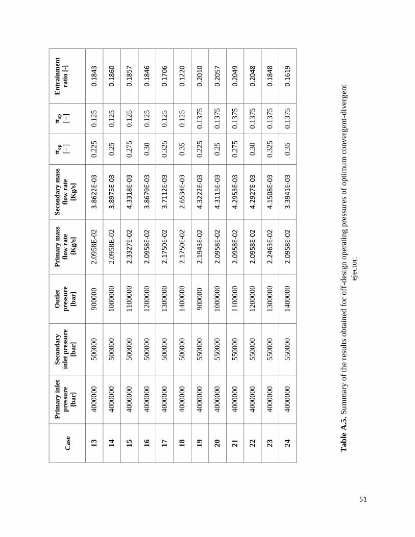
51

En

train

men

t

rati

o [

-]

0.1

843

0.1

860

0.1

857

0.1

846

0.1

706

0.1

220

0.2

010

0.2

057

0.2

049

0.2

048

0.1

848

0

.16

19

𝛑𝐬𝐩

[−]

0.1

25

0.1

25

0.1

25

0.1

25

0.1

25

0.1

25

0.1

375

0.1

375

0.1

375

0.1

375

0.1

375

0.1

375

𝛑𝐨

𝐩

[−]

0.2

25

0.2

5

0.2

75

0.3

0

0.3

25

0.3

5

0.2

25

0.2

5

0.2

75

0.3

0

0.3

25

0.3

5

Sec

on

da

ry m

ass

flo

w r

ate

[Kg

/s]

3.8

622

E-03

3.8

975

E-03

4.3

318

E-03

3.8

679

E-03

3.7

112

E-03

2.6

534

E-03

4.3

222

E-03

4.3

115

E-03

4.2

953

E-03

4.2

927

E-03

4.1

508

E-03

3

.39

41E-

03

Pri

ma

ry m

ass

flo

w r

ate

[K

g/s

]

2.0

958

E-0

2

2.0

958

E-0

2

2.3

327

E-02

2.0

958

E-02

2.1

750

E-02

2.1

750

E-02

2.1

943

E-02

2.0

958

E-02

2.0

958

E-02

2.0

958

E-02

2.2

463

E-02

2

.09

58E-

02

Ou

tlet

pre

ssu

re

[ba

r]

90000

0

10000

00

11000

00

12000

00

13000

00

14000

00

90000

0

10000

00

11000

00

12000

00

13000

00

14000

00

Sec

on

da

ry

inle

t p

ress

ure

[ba

r]

50000

0

50000

0

50000

0

50000

0

50000

0

50000

0

55000

0

55000

0

55000

0

55000

0

55000

0

55000

0

Pri

mary

in

let

pre

ssu

re

[bar]

40000

00

40000

00

40000

00

40000

00

40000

00

40000

00

40000

00

40000

00

40000

00

40000

00

40000

00

40000

00

Case

13

14

15

16

17

18

19

20

21

22

23

24

Tab

le A

.5.

Su

mm

ary o

f th

e re

sult

s ob

tain

ed f

or

off

-des

ign

op

erat

ing

pre

ssu

res

of

opti

mu

m c

on

ver

gen

t-div

erg

ent

ejec

tor.

52

REFERENCES

[1] DENSO Global Website. (2018). DENSO Develops World's First Passenger Vehicle Air

Conditioning System Using an Ejector | News | DENSO Global Website. [online] Available

at: http://www.globaldenso.com/en/newsreleases/090519-01.html [Accessed 14 Jun.

2018].

[2] Besagni, G., Mereu, R. and Inzoli, F. (2016). Ejector refrigeration: A comprehensive

review. Renewable and Sustainable Energy Reviews.

[3] Mazzelli, F. and Milazzo, A. (2015). Performance analysis of a supersonic ejector cycle

working with R245fa. International Journal of Refrigeration.

[4] Kadunic, S., Scherer, F., Baar, R. and Zegenhagen, T. (2014). Increased Gasoline Engine

Efficiency due to Charge Air Cooling through an Exhaust Heat Driven Cooling System.

MTZ worldwide.

[5] Greitzer, E., Tan, C. and Graf, M. (2004). Internal Flow: Concepts and Applications.

Refrigeración. Masters. Universitat Politécnica De Valencia, Departamento De Maquinas Y

New York: Cambridge University Press

[6] Ponce Mora, A. (2017). Optimización De La Geometría De Un Eyector Para Ciclos De

Motores Termicos, Escuela Técnica Superior De Ingeniería Del Diseño.

[7] Croquer, S., Poncet, S. and Aidoun, Z. (2016). Turbulence modeling of a single-phase

R134a supersonic ejector. Part 1: Numerical benchmark. International Journal of

Refrigeration.

[8] Su, Liju. (2015). "CFD SIMULATION AND SHAPE OPTIMIZATION OF SUPERSONIC

EJECTORS FOR REFRIGERATION AND DESALINATION APPLICATIONS".

Engineering and Applied Science Theses & Dissertations. 107.

http://openscholarship.wustl.edu/eng_etds/107.

[9] Zegenhagen, M. and Ziegler, F. (2015). Feasibility analysis of an exhaust gas waste heat

driven jet-ejector cooling system for charge air cooling of turbocharged gasoline engines.

Applied Energy.

[10] Zegenhagen, M. and Ziegler, F. (2015). Experimental investigation of the characteristics of

a ejector and a jet-ejector cooling system operating with R134a as a refrigerant. International

Journal of Refrigeration.