Geometric non-linear analysis of net structure

Master’s thesis Henrik Åkesson

Faculty of Engineering, LTH Department of Mechanical Engineering

Division of Mechanics

Abstract A geometric non-linear analysis of a net structure under constraints of maximum deflection is presented. The net is supported by fix attachment points. The fabric material behaviour is assumed to be linear elastic. The net is built from geometric non-linear truss elements and loaded by a constant load in one direction. The forces in the attachments points are determined. If is found that these forces are heavily dependent on the resulting net shape. It is also concluded that resulting forces are determined by the load distribution over the net.

b

Acknowledgments I would like to express my gratitude to Solveig Melin for her positive support and a big thank you to Majid Alavi who gave me the opportunity to work with his company, Telair International. A great thank you to Steen Krenk for supplying me with the chapters on non-linear trusses. Lund, Sweden 2007 Henrik Åkesson

c

Table of content 1 Introduction...................................................................................................................... 1 2 Objective .......................................................................................................................... 2 3 Choice of method............................................................................................................. 3 4 Preliminaries .................................................................................................................... 3 5 Nomenclature................................................................................................................... 4 6 Theoretical frame work.................................................................................................... 5

6.1 Non-linear trusses ..................................................................................................... 5 7 Numerical procedure........................................................................................................ 7

7.1 Non-linear routine..................................................................................................... 7 7.2 Line search ................................................................................................................ 9

8 The MATLAB program................................................................................................. 10 8.1 Calfem routines....................................................................................................... 10 8.2 Stifmatrix ................................................................................................................ 10 8.3 ElementP and ElementPf ........................................................................................ 10 8.4 AxialF ..................................................................................................................... 11 8.5 The geometry .......................................................................................................... 11 8.6 Deformations and original shape program.............................................................. 14 8.7 Blue print ................................................................................................................ 15 8.8 Cut routine .............................................................................................................. 16 8.9 Main interface ......................................................................................................... 17

9 Experimental testing ...................................................................................................... 20 9.1 Tensile testing ......................................................................................................... 20 9.2 Static test of net....................................................................................................... 21

10 Results.......................................................................................................................... 22 10.1 Linear CALFEM tests........................................................................................... 22 10.2 ANSYS tests ......................................................................................................... 23 10.3 Testing the MATLAB routine .............................................................................. 24 10.4 Final test................................................................................................................ 26

10.4.1 Ultimate load test ........................................................................................... 26 10.4.2 Single damage test ......................................................................................... 30

10.5 Pressure test .......................................................................................................... 32 11 Discussion .................................................................................................................... 34 12 References:................................................................................................................... 35 Appendix.............................................................................................................................. I

Huvudnet2........................................................................................................................ I stifmatrix ....................................................................................................................... III AxialF ........................................................................................................................... III ElementP ....................................................................................................................... III ElementPf...................................................................................................................... IV geometrinet2 ................................................................................................................. IV Oshapenet2f ............................................................................................................ XXXI ritningnet2 ............................................................................................................ XXXIV cutbeltnet2...................................................................................................................XLI

d

1 Introduction All areas of cargo handling have evolved during later years. For example, in shipping transport it started with men carrying by hand, but has now evolved to the employment of huge cranes lifting tons of cargo on to ships by the minute. In aircrafts the compartment of the narrow bodies was loaded by many men handing the baggage in a line, passing it forward in the narrow compartment. This cumbersome work is what Telair International has moved away from by producing a system that increases the loading and unloading efficiency which, in turn, reduces the ground time for the planes. Telair International installs a conveyer called the Sliding Carpet Loading System. This system utilizes a conveyer carpet that moves the baggage back in to the plane, handled by only one single worker - positioned by the cargo door - loading the baggage on to the conveyer carpet. After the baggage is put in to the hold a net is placed by the end of the conveyer carpet to secure the baggage in place. Their new system requires only one net as compared to old systems that utilized several nets. This requires a sturdier net because it is to hold the weight of all the baggage. Because only one net is used, the mounting points for the net are fewer. The planes were not originally constructed to secure the load with only one net so the loadings on the mounting points have to be carefully monitored in order not to exceed the limits for plastic deformation of the aluminium hull.

1

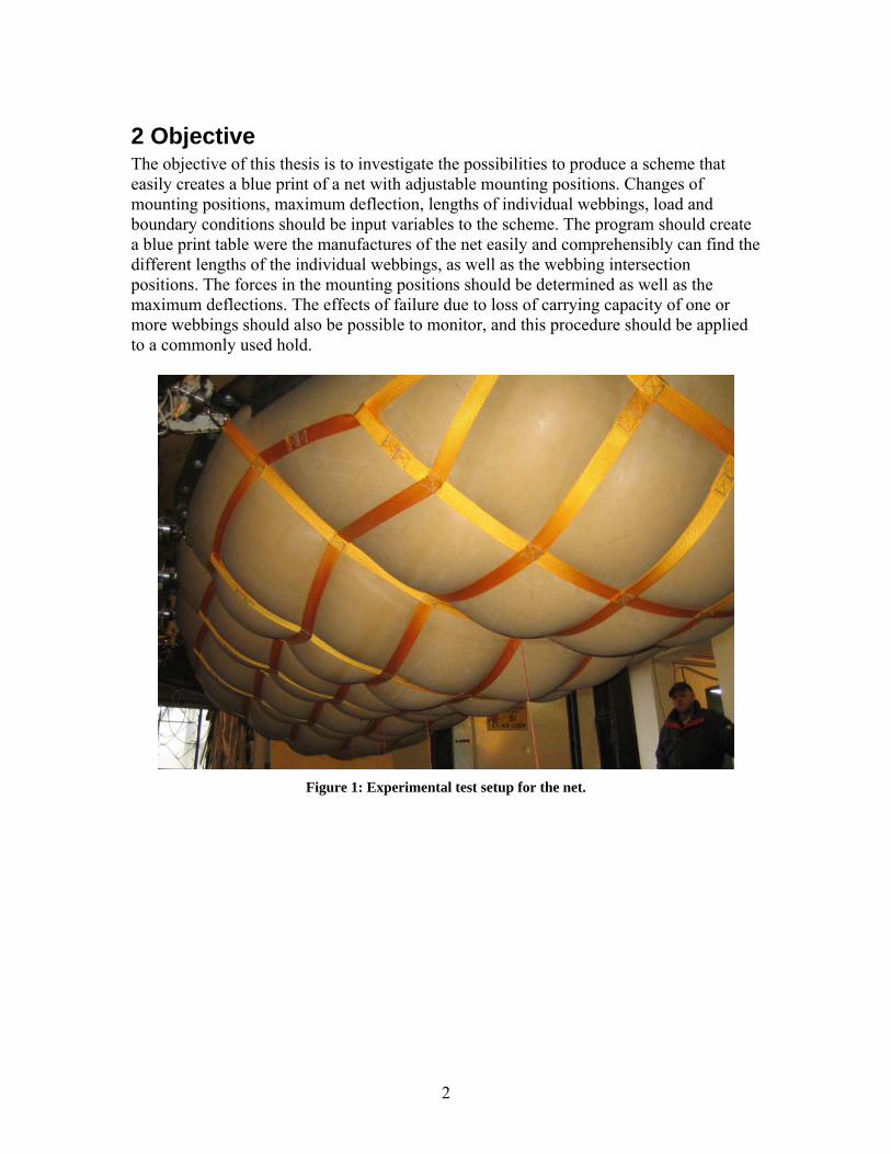
2 Objective The objective of this thesis is to investigate the possibilities to produce a scheme that easily creates a blue print of a net with adjustable mounting positions. Changes of mounting positions, maximum deflection, lengths of individual webbings, load and boundary conditions should be input variables to the scheme. The program should create a blue print table were the manufactures of the net easily and comprehensibly can find the different lengths of the individual webbings, as well as the webbing intersection positions. The forces in the mounting positions should be determined as well as the maximum deflections. The effects of failure due to loss of carrying capacity of one or more webbings should also be possible to monitor, and this procedure should be applied to a commonly used hold.

Figure 1: Experimental test setup for the net.

2

3 Choice of method Different numerical procedures were investigated to find a suitable approach to the problem. The outcome was that neither linear CALFEM calculations nor the commercial finite element code ANSYS, from different points of view, were found suitable. Instead, the net is modelled using the finite element code CALFEM with non-linear routines programmed in MATLAB. Each free part of the webbing consists of truss elements, and the intersections will be modelled momentum free. Loading will start from a shape of the net close to the original one (figure 2).

Figure 2: Original shape.

4 Preliminaries Telair International used two dimensional calculations to determine the net behaviour and, together with numerous tests, these calculations have resulted in information on how to manufacture the nets. A problem is that, with the two dimensional calculations, no information can be retrieved on how the deformation of one webbing interacts with other webbings, and how this in turn affects the mounting forces. A second problem is that there are some differences between plane types and there are many plane models. Telair International wants a program that, just by inserting new mounting positions and boundary conditions, can generate a new blueprint of a net which do not violate the boundary conditions. This would reduce the time the engineers would have to spend drawing/designing the blueprint. The program should be sufficiently accurate so that expensive testing could be minimized. It is here assumed that the reader of this thesis is familiar with basic finite element analysis and focus on the geometrically nonlinear parts will thus be prioritised. The theory is presented for a bar/truss element, which is the simplest element type because it deforms in only one degree of freedom. It has one internal force component in

3

its length direction, and the deformation is only in the length direction of the bar. Thus no shape function is needed for this element type. The equations used in the herein created code will be explained below by a simple truss model. The basic model will consist of two trusses. But the equations will, for the sake of clarity, be formulated for one truss, only.

5 Nomenclature l0 : Original length of the truss l: Deformed length of the truss a: Length in the y-direction b: Length in the x-direction u: Displacement a : Length vector of the truss u : Deformation vector ε : Strain N: Axial force in the truss E: Modulus of elasticity A: Cross sectional area of the truss P: External load K : Tangent stiffness matrix t

uΔ : Displacement increment : Load increment PΔ

R: Out-of-balance force Q: Internal force s: Line search parameter g : Gradient of potential energy sPf: Modified external load

4

6 Theoretical frame work

6.1 Non-linear trusses The stiffness matrix Kt applicable to the non-linear truss elements used in the formulation will be derived below. For further theoretical elaboration, cf. [3] and [5]. Consider a frame consisting of two truss elements according to figure 3. The free body diagram of one of the members is seen in figure 4. Let (x, y) be a Cartesian coordinate system with origin at the supported end (figure 4). Each member has the modulus of elasticity E, and the cross section area A. The projected length on to the horizontal is b and the initial vertical position of the joint is a, with a<<b. The displacement in the vertical direction is shown in figure 3.

Figure 3: Frame of two trusses.

Figure 4: Single truss.

The load P at the joint acts in the vertical direction. The original length of the bar is l0 and the deformed length is l, which gives

⎟⎟⎠

⎞⎜⎜⎝

⎛+≅+= 2

222

0 211

bababl (1)

5

( )⎥⎥⎦

⎤

⎢⎢⎣

⎡⎟⎠⎞

⎜⎝⎛ +

+≅++=2

22

211

buabuabl (2)

as obtained after series expansions where only second order terms are kept. A 3D equivalence to equations (1) and (2) can be arrived at as follows. Let the end points of the truss be ( )1111 ,, zyxa = ( )2222 ,, zyxa = and and the displacements at corresponding points ( )1111 ,, zyx uuuu = ( )2222 ,, zyx uuuu = and . Put

( ) ),,(;; 121212 zyx aaazzyyxxa =−−−= (3)

( ) ( ) ( ) ),,(];;[ 121212 zyxzzyyxx uuuuuuuuuu =−−−= (4) Then

2220 zyx aaal ++= (5)

( ) ( ) ( )222zzyyxx uauaual +++++= (6)

Because of large deformations there needs to be accountancy for changes in the engineering strain as compared to the linear form. The difference lies in the need to control the rigid body motion. The elongation consists of first a linear term and, second, a nonlinear term. Define the strain ε as

2

0000

0

21

⎟⎟⎠

⎞⎜⎜⎝

⎛+≅

−=

lu

lu

la

lll

ε (7)

which gives the axial force N in the truss equal to

⎥⎥⎦

⎤

⎢⎢⎣

⎡⎟⎟⎠

⎞⎜⎜⎝

⎛+≅=

2

000 21

lu

lu

laEAEAN ε (8)

Moment of equilibrium about the origin for one truss gives

( uauaulEA

luaNP +⎟

⎠⎞

⎜⎝⎛ +≅

+= 2

30 2

1 ) (9)

The stiffness matrix, Kt, is defined from infinitesimal changes in u and P giving the tangent stiffness

6

dudPKt = (10)

so that

2

0000⎟⎟⎠

⎞⎜⎜⎝

⎛ ++=⎟⎟

⎠

⎞⎜⎜⎝

⎛ +=

lua

lEA

lN

luaN

dudKt (11)

The first term corresponds to changes in the normal force and the second to changes in the geometric configuration.

7 Numerical procedure

7.1 Non-linear routine The non-linear solution scheme that will be used in this work utilizes the load history and, for each step, the displacements are calculated. For this, the non-linear equations are solved for the displacements employing an explicit increment method, cf. [5]. The procedure is a follows. First form (13) PKu t Δ=Δ −1

where ΔP is the load increment and Δu is the displacement increment produced by the load increment. The load and the displacement increment change iteratively so that, for n≥2,

nnn PPP Δ+= −1 (14)

nnn uuu Δ+= −1 (15) In the explicit incremental solution scheme the stiffness matrix is formed using the displacements at the previous increment. Then the displacement increment becomes

nntn PuKu Δ=Δ −− )( 1

1 (16) When using the previous step in forming the tangent stiffness matrix, a deviation from the actual solution results. This gives an error in the stiffness of the structure, and for every step this error builds up. The Newton-Rapshon method minimizes this error. This method checks if the solution is close enough to equilibrium and, if not, the displacements are recalculated using the current displacements to form a new stiffness matrix. This procedure proceeds until the solution is sufficiently close to equilibrium. In the code the first thing to be done is to check if the difference between the applied load (P) and the calculated load (Q) has reached the equilibrium condition (R). R is the residual force (out-of-balance load) in the structure, so that

7

(17) )(),( uQPPuR −= Q is calculated as Q(u)=P from equation (9). In the first step the load is applied, which pushes the system out of equilibrium. To reach a new equilibrium state, iterations have to be performed. With the residual force a new displacement increment can be calculated in each iteration, i.e.

RuKu ntn )( 11

−−=Δ (18)

Here the tangent stiffness matrix is a derivative of the internal force as shown above, cf. equation (11). This displacement increment is used to update the displacement:

iii uuu Δ+= −1 (19) where ui-1 is the displacement calculated in the previous iteration. The iteration has a termination criterion that stops the iteration when a state, sufficiently close to equilibrium, is reached. In the final routine the termination criteria checks the residual force, and if it is sufficiently small or when the number of iterations has exceeded some predetermined number, the calculations stop. For every step new values for the normal force and the internal force are calculated, and these values are used in the calculations of the tangent stiffness matrix and in the residual force vector. The algorithm for the Newton-Raphson method and how the iteration scheme works during one load step can be seen below. Here P , ΔPn is a vector containing all the force components Pn n is an applied load increment vector, Rn is the out-of-balance force vector, Q is the calculated nodal force vector, K is the tangential stiffness matrix, and δun n is the displacement increment vector. The notation ||x|| denotes the norm of the vector x, cf. [5]. Newton-Raphson iteration scheme:

= PPn n-1+ΔPn R =P -Q(u ) n n n-1Iterations (||R ||< η ||ΔP ||) (η is the tolerance) n n Kn=dQ(un-1)/du R =P -Q(un n n)

-1 δu =K Rn n n u = u + δun n n end iteration

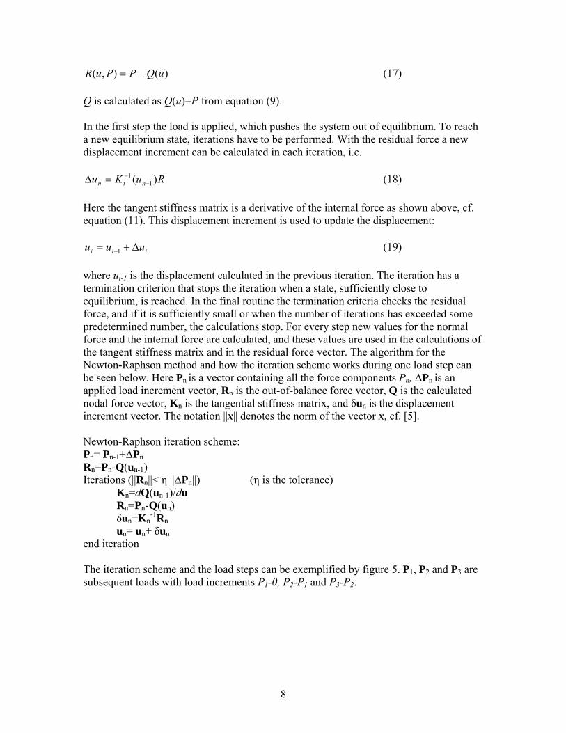
, PThe iteration scheme and the load steps can be exemplified by figure 5. P1 2 and P3 are subsequent loads with load increments P1-0, P -P and P2 1 3-P . 2

8

Figure 5: Newton-Raphson iteration scheme with load increments.

In the modified Newton-Raphson method the calculation of the tangent stiffness matrix is moved outside the iteration loop. This makes the iteration faster but the asymptotic convergence slower. For problems with many degrees of freedom use of the modified Newton-Raphson method can be faster, however, and therefore advantageous.

7.2 Line search For the ANSYS [14] tests the line search function was used. In terms of above equations the displacements can be expressed as

iii uuu Δ+=+1 (20) If, during iteration, it is found that the prescribed step Δui gives unstable solutions, a modification reducing Δui by the scalar factor s, named the line search parameter and with 0.05<s<1.0, is introduced:

iii usuu Δ⋅+=+1 (21) s can be determined by minimizing the energy of the system. This is done by finding the zero of the non-linear equation:

( )( )inraT

is usFFug Δ⋅−Δ= (22) where gs is the gradient of the potential energy with respect to s, Fa applied loads, Fnr restoring loads corresponding to the element internal loads and ΔuT

i denotes the transpose of the vector Δui. This equation is solved with an iterative solution scheme available in ANSYS.

9

8 The MATLAB program

8.1 Calfem routines Assem: Assembles the stiffness matrix in to a global matrix. (Ref. 2) eldisp3: Displays the 3D deformed shape. coordxtr: Extracts the elements coordinates from the Coord matrix using Edof.

(elements degrees of freedom) and Dof (degrees of freedom). solveq: Solves static FEM equation producing the new deformation change. extract: Extracts the elements deformations. insert: Inserts forces in to a global force vector.

8.2 Stifmatrix Stifmatrix is the MATLAB routine used to form the tangential stiffness matrix for one element and all elements are sorted into the global stiffness matrix. The routine utilizes the following form of the stiffness matrix:

2

000⎟⎟⎠

⎞⎜⎜⎝

⎛ ++=

lua

lEA

lNKt (23)

8.3 ElementP and ElementPf ElementP calculates the nodal forces for one element. The following equation, equation (24):

luaNP +

= (24)

has been transformed into 3D space to read:

a uP Nl+

= (25)

It was noted that if l was replaced by l0 to form the following equation, this helped the system to converge. This defines Pf .

0luaNPf +

= (26)

This modification made the system converge faster, which meant that the solution could be reached faster. The solution is not accurate, though, since the normal forces (N) and the tangential stiffness matrix where incorrect. The nodal forces (P=(Px,Py,Pz)), however, turned out to be correct, most likely as a result of the fact that the solution procedure is force controlled. Even so equation (26) could be used to make the system converge faster. So the quantity Pf was used when creating the starting shape. Once the system has

10

reached convergence this convergence is not breached when changing the elements nodal force equation. Because there is a major problem with convergence in the first steps, this is extremely helpful. This quantity is also used in the cut programdescribed below. In the program, ElementPf replaces ElementP until the system has converged.

8.4 AxialF The MATLAB routine AxialF calculates the normal forces for the elements. This is done by equation (27):

⎥⎥⎦

⎤

⎢⎢⎣

⎡⎟⎟⎠

⎞⎜⎜⎝

⎛+≅

2

000 21

lu

lu

laEAN (27)

8.5 The geometry The design of the net geometry is similar between planes, except for the coordinates of the mounting points. Thus the variables are the mounting points. A geometry file, written in MATLAB, takes care of producing a starting geometry which can be exposed to loading. The variable names and the coordinate system are shown in figure 6. This starting geometry is used in a program that deformes it in the load direction to get the original net geometry and the final, deformed geometry. The program needs also to have different degrees of resolution, meaning that the number of elements in the net are possible to modify. This is important because when optimising the net, fewer elements can be used to make the calculations faster. But for the calculations on the final net, smaller and more elements are required. Thus the number of elements in the net and in the mounting can be changed. The mounting of the net in the plane and the changes this induces to the net dimensions had to be considered, so the mounting and its size are two more variables than can be changed. There are two parts of mounting; one metal lock that locks the net in place and one additional piece of webbing that connects the net to the locking device. Both of these changes the net geometry. In the MATLAB geometry file, first the coordinates of the nodes are created. The coordinates of the nodes are collected in the Coord matrix. The coordinates are then bound together to form elements. The elements are saved in the Edof matrix, where elnr is the element number, and dofnr and dofnr2 are the numbers of degrees of freedom number for the elements. All the variables that start their name with dof are the degrees of freedom number for a certain node. For example, dofCsm is the degree of freedom for the x direction of the C position, and the s denotes that it is the C point on the side where the value of x-position is negative. The m denotes that it is on the net and not on the mounting point. The next step is to save the z-degrees of freedom for the different webbings so that they can be individually deformed later when the optimization of the net is performed. This is also used when applying the load. The load is only applied on the net, and not on the mounting webbing. This is because one could choose a lot of elements in the mounting webbing sections, resulting in distortion of the load disruption. The load does not use a

11

Lagrangian formulation, it is just split on to the nodes and the same amount of load is applied on each node in the net. The degrees of freedom of the mounting points are saved in bc and are used for setting the boundary conditions. The variable Nele is the number of elements for the geometry and Nnoder is the number of nodes. The matrix called Dof holds the degrees of freedom for each node. All of these matrixes are used to get the positions of the elements and this is done by the CALFEM routine called coordxtr.

12

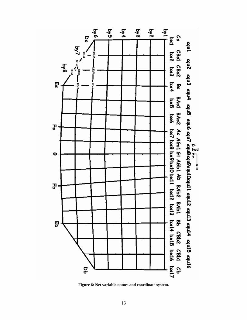
Figure 6: Net variable names and coordinate system.

13

8.6 Deformations and original shape program To get the final shape, the forces and the maximum deflection, the iteration procedure explained in the theory section has been used, and all though some modifications have been made, the procedure is basically the same. Some of the variables and options are retrieved from the interface file (se below) and the matrixes needed for the geometry are imported from the geometry file. The first step in the program is to move the webbings as much as the user has specified. These movements are mostly in the plane of the net so the distances between webbings do not exceed the specified limit given by the airplane manufactures. These movements are made before the net has been given its final shape. Because the final net configuration is so complicated, the shape is produced by first creating a flat net that gets its final shape by the application of forces. To get a final shape that gives optimal forces in the mounting points, webbings can be moved before the loads that give the original shape are applied, and the forces that give the desired shape can be modified so that some webbings stretch more. The net nodes are subjected to forces that always have the same direction, namely the z-direction. The Pb force is the force that initially shapes the net (original shape) and the weight is the force that is the actual load that is applied to the net. To get the maths to work, the normal force (N) in the bars needs to be non-zero, so the normal forces are set to some small value prior to the first step. The iteration procedure comprises of two different load applications. The first load creates the original shape and the second one is for the weight. The second is performed within the shape iteration and the reason for this will be explained later. First the shape iteration takes one load step, and then the weight is applied in steps until the entire load has been applied. First thing is to make sure that the load steps stop when the maximum deflection has been reached. But because the first load step/steps can produce incorrect results, load steps for the original shape will continue until convergence. Numerical problems in the first step have to do with the stiffness of the structure. When the net is flat, the stiffness is very low, and a small load will make it deflect extremely. The theory states that a small load increment should be added each step. I have used that in a MATLAB routine:

iPP start *= equivalent to (28) )()1()( iii PPP Δ+= −

where P is the load, ΔP is a small load increment, and Pstart is equivalent to ΔP. The difference between the formulations in (28) is that Pstart is a vector and ΔP is a scalar and i is the number of the current step. This approach has been used because it is easier to keep track on the loaded nodes if they are assigned a value already in the first increment. The webbings that needs to be modified are each loaded with their extra load.

14

R is the residual force that is produced by subtracting the internal force from the applied force. All the degrees of freedom of the mounting points are set to zero to match the boundary conditions. Niter is the maximum number of iterations that can be performed for each load step. This is important to include because some load steps (i.e. the first) might not converge. The iteration starts by creating the tangent stiffness matrix. With this and the residual force vector a new shape/deformation is produced. For the next step the normal force (N) and the internal forces (Q) have to be calculated with the use of the new shape/deformation, giving an original shape of the net. This means that the net now has a shape that can be deformed by the weight. This leads to the second phase. The deformations are added on to the starting shape and then this shape is deformed by the weight. After this the maximum deflection is checked. If the largest deflection has not reached the maximum deflection the original shape is deformed further with a load step. The weight iterations is only performed if the starting shape has converged. For every step the maximum deflection and the number of iterations are presented in the command window in MATLAB. This is important to observe because if the number of iterations is the same as the maximum number, the iteration has not converged. If the iteration has converged but the maximum deflection has been exceeded by too much, smaller load increments should be used for the forming of the original shape.

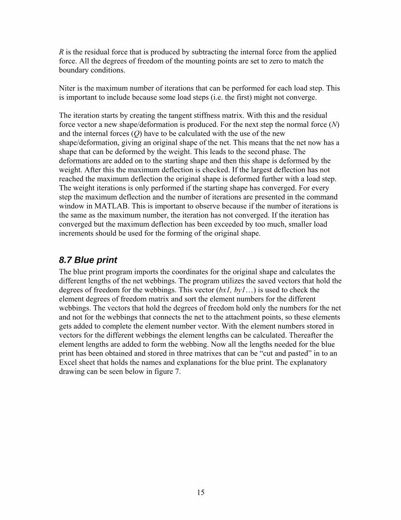
8.7 Blue print The blue print program imports the coordinates for the original shape and calculates the different lengths of the net webbings. The program utilizes the saved vectors that hold the degrees of freedom for the webbings. This vector (bx1, by1…) is used to check the element degrees of freedom matrix and sort the element numbers for the different webbings. The vectors that hold the degrees of freedom hold only the numbers for the net and not for the webbings that connects the net to the attachment points, so these elements gets added to complete the element number vector. With the element numbers stored in vectors for the different webbings the element lengths can be calculated. Thereafter the element lengths are added to form the webbing. Now all the lengths needed for the blue print has been obtained and stored in three matrixes that can be “cut and pasted” in to an Excel sheet that holds the names and explanations for the blue print. The explanatory drawing can be seen below in figure 7.

15

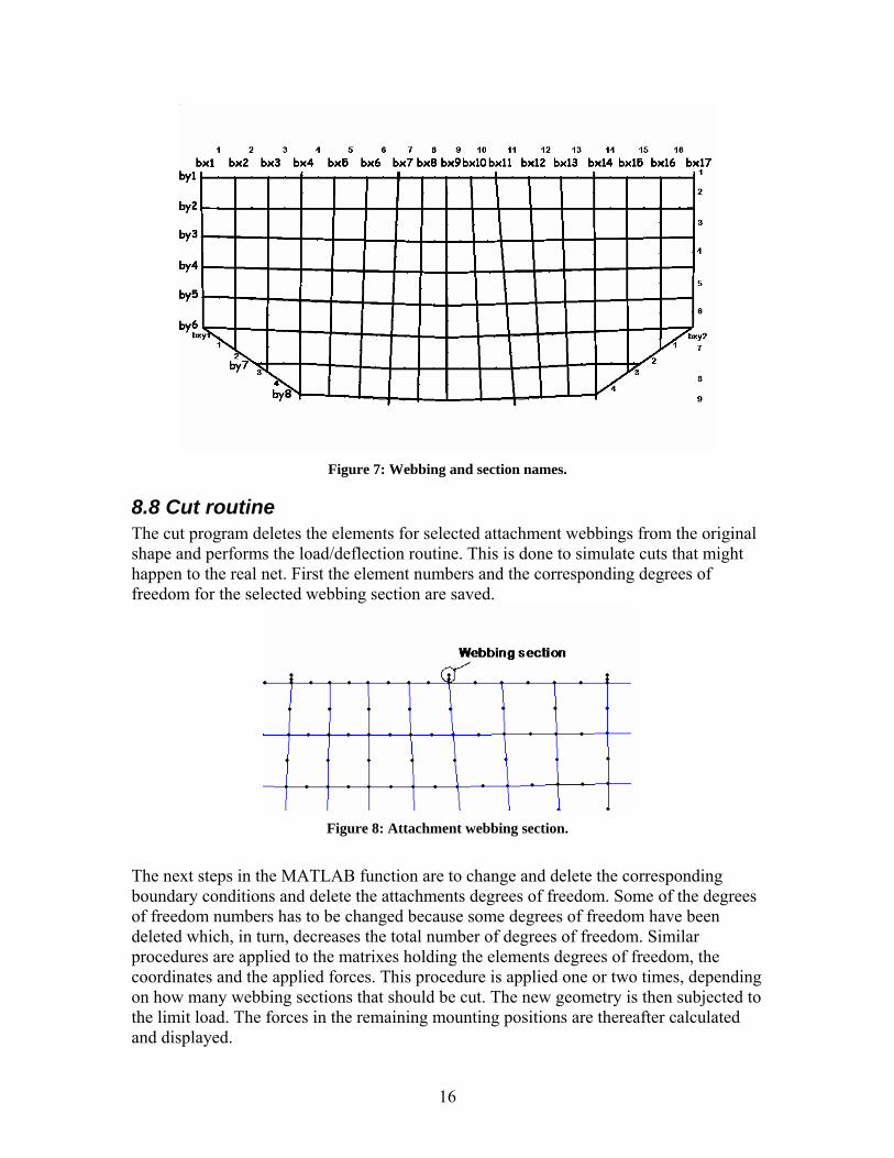
Figure 7: Webbing and section names.

8.8 Cut routine The cut program deletes the elements for selected attachment webbings from the original shape and performs the load/deflection routine. This is done to simulate cuts that might happen to the real net. First the element numbers and the corresponding degrees of freedom for the selected webbing section are saved.

Figure 8: Attachment webbing section.

The next steps in the MATLAB function are to change and delete the corresponding boundary conditions and delete the attachments degrees of freedom. Some of the degrees of freedom numbers has to be changed because some degrees of freedom have been deleted which, in turn, decreases the total number of degrees of freedom. Similar procedures are applied to the matrixes holding the elements degrees of freedom, the coordinates and the applied forces. This procedure is applied one or two times, depending on how many webbing sections that should be cut. The new geometry is then subjected to the limit load. The forces in the remaining mounting positions are thereafter calculated and displayed.

16

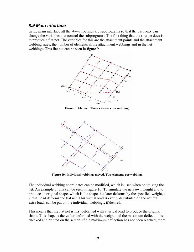
8.9 Main interface In the main interface all the above routines are subprograms so that the user only can change the variables that control the subprograms. The first thing that the routine does is to produce a flat net. The variables for this are the attachment points and the attachment webbing sizes, the number of elements in the attachment webbings and in the net webbings. This flat net can be seen in figure 9.

Figure 9: Flat net. Three elements per webbing.

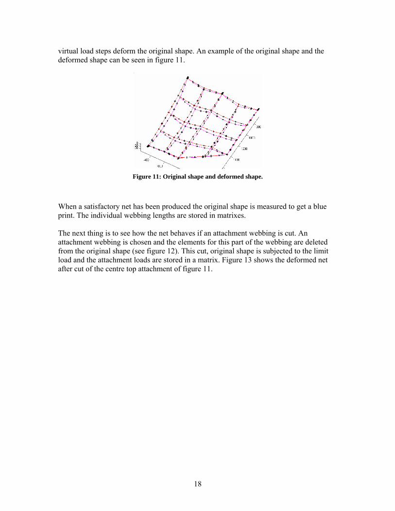
Figure 10: Individual webbings moved. Two elements per webbing.

The individual webbing coordinates can be modified, which is used when optimizing the net. An example of this can be seen in figure 10. To simulate the nets own weight and to produce an original shape, which is the shape that later deforms by the specified weight, a virtual load deforms the flat net. This virtual load is evenly distributed on the net but extra loads can be put on the individual webbings, if desired. This means that the flat net is first deformed with a virtual load to produce the original shape. This shape is thereafter deformed with the weight and the maximum deflection is checked and printed on the screen. If the maximum deflection has not been reached, more

17

virtual load steps deform the original shape. An example of the original shape and the deformed shape can be seen in figure 11.

Figure 11: Original shape and deformed shape.

When a satisfactory net has been produced the original shape is measured to get a blue print. The individual webbing lengths are stored in matrixes. The next thing is to see how the net behaves if an attachment webbing is cut. An attachment webbing is chosen and the elements for this part of the webbing are deleted from the original shape (see figure 12). This cut, original shape is subjected to the limit load and the attachment loads are stored in a matrix. Figure 13 shows the deformed net after cut of the centre top attachment of figure 11.

18

Figure 12: Deleted attachment webbing within circle.

Figure 13: Deformed shape after the cut.

19

9 Experimental testing

9.1 Tensile testing Experiments were conducted so that a value of the Young’s modulus (E) could be obtained. The webbing used in the net was tested using a sample piece. The sample dimensions and its layout can be seen in figure 14, where the squares are the stitching and the webbing is folded double except for the centre section that is 2x165 mm long. Because some sections are folded double, the final displacement magnitude has been modified so that only the deformations in the 2x165mm sections are taken account of. This is done by certain recalculations made at Telair International.

Figure 14: Blue print of the sample piece.

The result from the experiment can be seen in figure 15, were the non-linear curve is from the testing. The linear curve is a product of the non-linear finite element equations. This gives an estimated E-modulus of 6.8 ·108 Pa. The material and the stitching of the webbings give a non-linear material behaviour but in this thesis it will be assumed that the material can be modelled with a constant E-modulus.

20

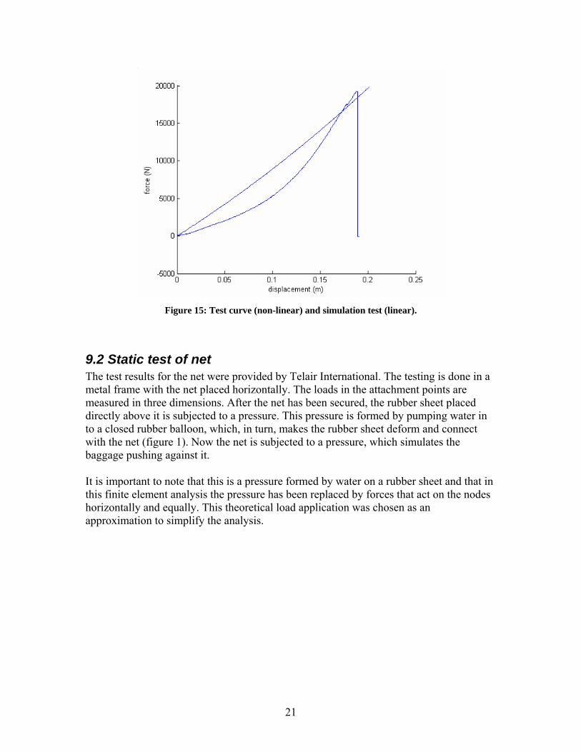
Figure 15: Test curve (non-linear) and simulation test (linear).

9.2 Static test of net The test results for the net were provided by Telair International. The testing is done in a metal frame with the net placed horizontally. The loads in the attachment points are measured in three dimensions. After the net has been secured, the rubber sheet placed directly above it is subjected to a pressure. This pressure is formed by pumping water in to a closed rubber balloon, which, in turn, makes the rubber sheet deform and connect with the net (figure 1). Now the net is subjected to a pressure, which simulates the baggage pushing against it. It is important to note that this is a pressure formed by water on a rubber sheet and that in this finite element analysis the pressure has been replaced by forces that act on the nodes horizontally and equally. This theoretical load application was chosen as an approximation to simplify the analysis.

21

10 Results

10.1 Linear CALFEM tests The first tests with finite elements were made in MATLAB with 2D linear elements and a parabolic starting shape of one webbing section. These tests could then be compared to the calculations Telair international had provided. With linear elements and a parabolic starting shape the linear finite element calculations give the following deformed shapes after the webbing has been subjected to a distributed force of constant magnitude in the downward direction, cf. figures 16 and 17.

Figure 16: Linear beam elements.

Figure 17: Linear truss elements.

Two different element types were tested and the resulting shapes are shown in figure 16 and figure 17. In figure 16 beam elements and in figure 17 truss elements were used. As can be seen both these element types procedure diverge from the desired parabolic shape. The conclusion is that a MATLAB routine with nonlinear elements needs to be developed. This task is the object of the present thesis.

22

10.2 ANSYS tests There were no nonlinear elements in CALFEM that could be used, so tests with a nonlinear solution procedure were first made in ANSYS [14]. The geometries were generated in MATLAB. The commands used specially for the nonlinear procedure were; nlgeom to state that it was a nonlinear geometry, link10 was chosen as element type and lnsrch was used to utilize line search. No converged solution was obtained without line search. There was no need to use the correct E-modulus for this numerical test, E was simply chosen so that the applied load gave the correct maximum deflection. The forces and deflections were compared with the data given by Telair International. The differences between results, in %, can be seen in Table 1, where h is the maximum deflection, T0 is the force in the horizontal direction and Fx is the vertical force at the endpoints according to figure 18. The E-modulus was chosen to minimize the difference in the deflection for the 20 element test, and then kept the same for all other tests.

Figur 18: The webbing deflection and force definitions.

Number of elements 20 10 4 h(%) 0.12 2.38 11.87 T (%) 1.41 1.68 12.23 0F (%) 0.13 0.13 0.13 x

Table 1: ANSYS test, single webbing (%).

Telair international required that the difference should not exceed 5%. The results were below this limit when sufficiently many elements were used as seen from Table 1. ANSYS tests on a net were also performed to make sure that calculations such as conducted in this thesis on the extremely complex net geometry could converge, and that it would be possible to avoid numerical stability problems. The result can be seen below, and in the net in figure 19, only one element is used for each section.

23

1

DEC 5 200614:39:43

DISPLACEMENT

STEP=1SUB =8TIME=1DMX =206.627

Figur 19: ANSYS test, deformed net.

These positive outcomes of the ANSYS calculations indicated that it should be possible to write a non-linear MATLAB routine to simulate net deformations.

10.3 Testing the MATLAB routine The ANSYS single webbing tests illustrated in figure 18 were repeated for the MATLAB routine developed in this thesis. The results are shown in Table 2. Additionally, for the 20 element test, the difference in the angle in the mounting point was 0.12°, and for the 10 element test it was 1.07°. As seen from Table 2 the accuracy is higher using the present MATLAB routine than using ANSYS with the same number of elements. Number of elements 20 10 4 h(%) 0.06 1.96 9.6 T (%) 0.46 3.71 13.3 0F (%) 0.0 0.0 0.0 x

Table 2: MATLAB test, single webbing (%).

It is clear that the number of load steps and the maximum number of iterations are closely connected. Smaller load steps helps the system to convergence faster, but more load steps means that the iteration procedure has to be repeated more times. An investigation was therefore undertaken to see how many steps/iterations was needed to make T0=1754.8 N, as measured in experiments, using 20 elements. Figure 20 shows how the number of steps and the number of iterations are intertwined.

24

Figure 20: Relation between number of steps and number of iterations.

The result depends on the resolution of the net, i.e. how many elements that are used for each webbing. Maximum number of iterations was set to 40, convergence tolerance 10-8 and number of steps to 200. Figure 21 shows how the accuracy depends on the number of elements.

Figure 21: Number of elements and its effects on the accuracy.

25

10.4 Final test The final test was to see if the finite element net matched the experimentally tested net. The net used was somewhat different than the net used when the MATLAB functions was originally written. This meant that a new net had to be produced. This in itself turned out to be a useful test, as to see how long it takes to produce a new net structure. The changes were made in the geometry, blue print and the cut routine, with the emphasis on the geometry function. This took approximately one day, using the old MALAB-code followed by copy/paste and changing the variable names. Running the program and optimizing the net can take some time but, depending on computer capacity, this is more a job for the computer than for the engineer. In the final net the E-modulus was set to 10·108 Pa (test 6.8 ·108 Pa, cf figure 15). This was done because the test showed that the maximum deflection would be exceeded with the linear approximation of the E-modulus obtained by simulations. Anyhow, the material of the net is highly non-linear and this slight increase in E-modulus is not critical. In the real net there is one webbing that goes Es-Ds-Db-Eb (figure 6) that freely can move in the D point. In the finite element analysis net this webbing is split into Es-Ds, Ds-Db and Db-Eb. This means that the forces in D and E become incorrect, which should be observed when interpreting the results.

10.4.1 Ultimate load test The largest forces and the most interesting ones are in the centre of the net and especially the force components in the y- and z-directions. Figure 22 shows the differences between the finite element analysis and the experiments. The figures shown starts on top with the force in the x-direction and goes down to y, z, and single (the 2-norm ||x||2, cf [15]) force within brackets. Each figure shows how many times larger/smaller the simulation result is compared to the experiments, i.e. simulation result divided by experimental result.

26

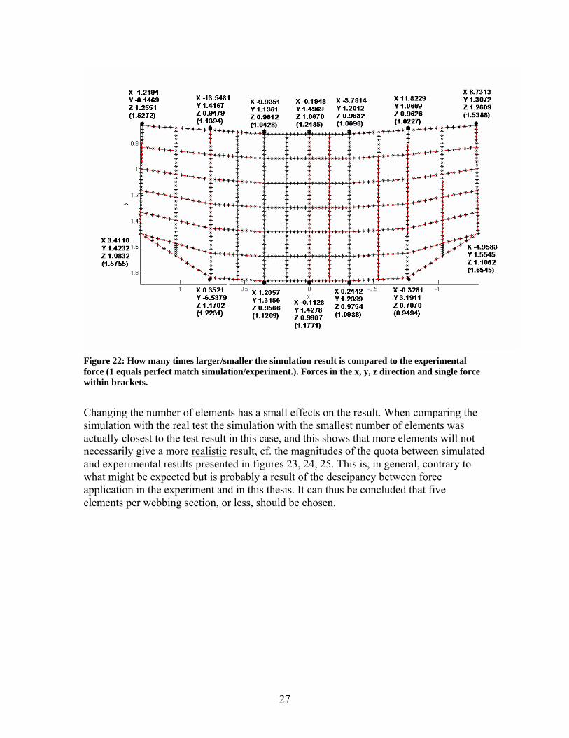
Figure 22: How many times larger/smaller the simulation result is compared to the experimental force (1 equals perfect match simulation/experiment.). Forces in the x, y, z direction and single force within brackets.

Changing the number of elements has a small effects on the result. When comparing the simulation with the real test the simulation with the smallest number of elements was actually closest to the test result in this case, and this shows that more elements will not necessarily give a more realistic result, cf. the magnitudes of the quota between simulated and experimental results presented in figures 23, 24, 25. This is, in general, contrary to what might be expected but is probably a result of the descipancy between force application in the experiment and in this thesis. It can thus be concluded that five elements per webbing section, or less, should be chosen.

27

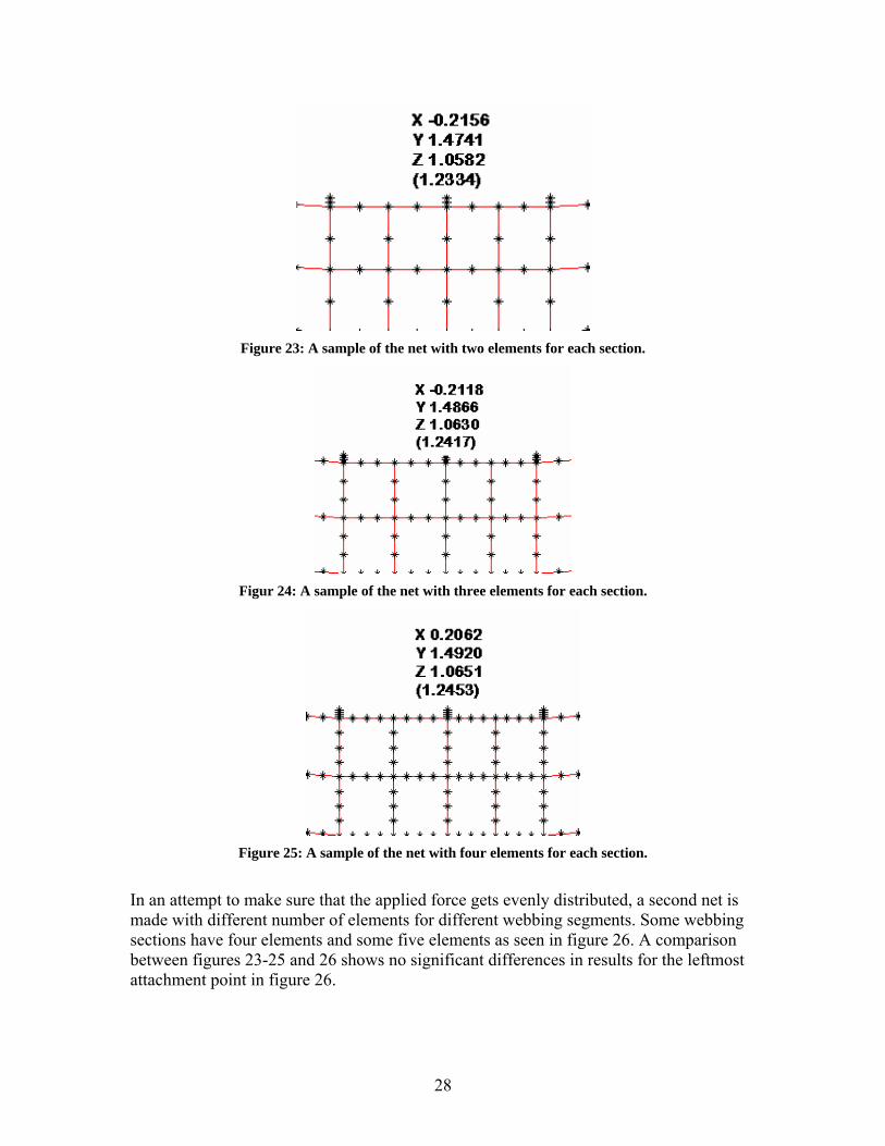
Figure 23: A sample of the net with two elements for each section.

Figur 24: A sample of the net with three elements for each section.

Figure 25: A sample of the net with four elements for each section.

In an attempt to make sure that the applied force gets evenly distributed, a second net is made with different number of elements for different webbing segments. Some webbing sections have four elements and some five elements as seen in figure 26. A comparison between figures 23-25 and 26 shows no significant differences in results for the leftmost attachment point in figure 26.

28

Figure 26: A sample of the net with different amount of elements for different parts of the sections.

The figures below show the deformed net from different angles. The simulated shapes in figures 27 and 28 can be compared to figure 29. In figure 28 attention should be given to the fact that the centre of the net is not deformed in the same way as the real net. This is accredited to the fact that the load application differs between the simulations and the experimental setup.

Figure 27: View of the net.

Figur 28: Side view of the net.

29

Figur 29: Deformed net, real testing.

10.4.2 Single damage test One attachment webbing is cut and a lower load, the limit load, is applied. When the cut is made at any of the positions E, D, and/or C ,c.f. figure 6, the numerical calculations in the routine will converge slower. If the original shape was chosen so that no deformation and, therefore, no converged shape had been reached before cutting the attachment webbing, the program had problems finding a converged form from the cut net routine.

Figure 30: A net with single damage. Forces in the x, y, z directions and single force (||x||2) within brackets.

30

The maximum deflection for the single damage test was 367.6 mm. Figures 31, 32 and 33 show the deformed net with a single damage.

Figur 31: Side view of a net with a single damage.

Figur 32: Top view of a net with a single damage.

Figur 33: View of a net with a single damage.

31

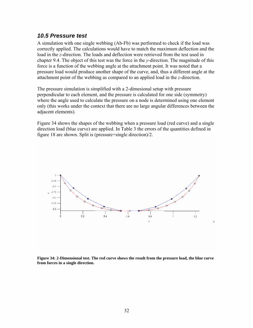
10.5 Pressure test A simulation with one single webbing (Ab-Fb) was performed to check if the load was correctly applied. The calculations would have to match the maximum deflection and the load in the z-direction. The loads and deflection were retrieved from the test used in chapter 9.4. The object of this test was the force in the y-direction. The magnitude of this force is a function of the webbing angle at the attachment point. It was noted that a pressure load would produce another shape of the curve, and, thus a different angle at the attachment point of the webbing as compared to an applied load in the z-direction. The pressure simulation is simplified with a 2-dimesional setup with pressure perpendicular to each element, and the pressure is calculated for one side (symmetry) where the angle used to calculate the pressure on a node is determined using one element only (this works under the context that there are no large angular differences between the adjacent elements). Figure 34 shows the shapes of the webbing when a pressure load (red curve) and a single direction load (blue curve) are applied. In Table 3 the errors of the quantities defined in figure 18 are shown. Split is (pressure+single direction)/2.

Figure 34: 2-Dimensional test. The red curve shows the result from the pressure load, the blue curve from forces in a single direction.

32

Pressure Single direction Split h(%) 0.9 0.6 T (%) 32 -24 4 0F (%) 0.07 -2 x

Table 3: The difference (%) between the real test and the different load situations.

Table 3 shows that neither one of the approaches is more correct than the other. The results from the real test can be found in between the two. This means that the experimental test load most probably is a mixture of a one directional load and a pressure load.

33

11 Discussion The maximum number of iterations should be high to make sure the system finds equilibrium. Once equilibrium has been reached, the number of iterations will decrease. The magnitude of the load increment of each load step for the starting geometry should be relatively high so that the number of steps is kept down. More steps means that the loading phase is repeated more times and this will slow down the solution procedure. But if the magnitude is too large it will cause problems in the iteration phase and one might over-shoot the maximum deflection. The number of maximum iterations and step sizes has to be adjusted to an adequate level. The number of elements used for the geometry has little effect on the number of iterations or the step size. So the same number of iterations can be used when using more elements to model the webbings. The elasticity modulus must be re-evaluated so the simulation matches the real tests. Consideration should be made to the difference in how the loads are applied in the test and in the simulation. In the real test the load is a pressure, but in the finite element simulation nodal forces working in the z-direction are applied. In the real test the rubber sheet edges are clamped down. This, and the fact that pressure in this area is acting more in the y-direction, produce different results as compared to the simulations. This can be seen by the fact that the simulations show higher forces acting in the x-direction. It also shows when looking at the test photo and comparing the edges of the net with the simulation. The best thing would be to change the load direction and use a function that simulates the water pressure. This would make the simulated resluts come closer to the test. The real test has pressure acting in all directions, so the net will not deform in the same way as in the simulation. The pressure acting on the net will give different normal forces in the webbings; this in turn produces different deformations which, in turn, are controlled by the E-modulus. This means that the non-linear E-modulus given by the test should be used instead of a constant value. When Pf was used for a single webbing test it only needed one fourth of the steps as compared to the calculations with P used. Although Pf gives wrong results, the final result will be correct. This is under the assumption that sufficiently many converged steps have been taken. Pf helps the calculations reach a converged form and after that, the real P can be used in the calculations. The results for the forces in the x- and y-directions show that the MATLAB routine is flawed. The reason why the simulation and the reality are different is probably mainly due to that the test uses a rubber sheet to apply the load whereas in the simulation the forces acts on the nodes in one of the three degrees of freedom. The first step that should be taken to improve the simulations would be to use a pressure load that is distributed on the net in a similar way to that seen in the experimental setup. Using a Lagrangian way to distribute the loads could also be of help. The vectors that hold the node numbers for the individual webbings can be used to calculate the angles and lengths used when determining the pressure distribution and the Lagrangian forces.

34

12 References: 1. Niels Ottosen & Hans Petersson, University of Lund, Introduction to the finite

element method. ISBN 0-13-473877-2 2. CALFEM – a finite element toolbox to MATLAB version 3.3, (2002), Division of

Structural Mechanics and Division of Solid Mechanics, LTH. 3. M. A. Crisfield, Non-linear finite element analysis of solids and structures,

volume 1. ISBN 0-471-97059-X 4. M. A. Crisfield, Non-linear finite element analysis of solids and structures,

volume 2. ISBN 9780471956495 5. Steen Krenk - Non-Linear Modelling and Analysis, DTU, Denmark 6. Gert Nilson, , The belt-in-seat concept mathematical modelling of protective

effects. 7. Katarina Blom, Fortran 90 – en introduction. ISBN 91-44-47881-X 8. Koffman, Friendman, Fortran fifth edition update. ISBN 0-201-59062-X 9. Ola Öhrström, Finite element formulation for shells and thin walled beams, linear

and geometric non-linear analysis. Lund 1995, Report TVSM, 5060 10. Tsu-Wei Chou and Frank K. Ko, Textile structural composites, volume 3

composite materials series. Amsterdam : Elsevier, 1989 11. Jiri Havir, Licentiate Thesis, Division of Solid Mechanics (2005) LTH, Om

kantbuckling av pappersbanan vid pappersproduktion. 12. F. L. Román, J. Faro, and S. Velasco, Departamento de Fisica Aplicada, A simple

experiment for measuring the surface tension of soap solutions. Departamento de Fı´sica Aplicada, Facultad de Ciencias, Universidad de Salamanca, 37008 Salamanca, Spain

13. Anders Gavelin, Luleå University of Technology, Seat integrated safety belts A

parametric study using finite element simulations. ISSN 1402-1757 / ISRN LTU-LIC--06/21--SE / NR 2006:21

14. ANSYS 10.0 University Advanced 15. Endre Süli and David Mayers, An introduction to Numerical Analysis. Cambridge

university press, ISBN 0 521 81026 4

35

36

Appendix

Huvudnet2 uMax=-0.316; Pb=-1000; %The weight used to create the original shape Ef=10e8; %The E-modulus used to create the original shape ep=[Ef 1]; weight=-69873; %The real weight E=10e8;%6.8e8; %The E-modulus used for the net A=0.025*0.002; %Cross section area that goes together with the E-modulus above eps=[E A]; Steps=60; %Maximum number of iteration steps intmax=1000; %Maximum number of iteration outTol=1e-6; %error tolerance Nsq=1; %Nsq=1,2,3...Number of nodes in the net sections Ninf=1; %Number of nodes in the attachment webbing shapeForce=0; %1=true 0=false shape and force BluePrint=1; %1=true 0=false blueprint cutTheBc=0; %1=true 0=false run cutbelt nodcut1='Es'; %a string As,Ab,Bs,Bb,Es,Eb,Fs or Fb delets the elements for the mounting belts. nodcut2=0; %If 0 (zero) only one cut, 2cut use the same strings as above As=[0,0,0]*0.001; Ab=[0,0,0]*0.001; Bs=[0,0,0]*0.001; Bb=[0,0,0]*0.001; Cs=[0,0,0]*0.001; Cb=[0,0,0]*0.001; Ds=[0,0,0]*0.001; Db=[0,0,0]*0.001; Es=[0,0,0]*0.001; Eb=[0,0,0]*0.001; Fs=[0,0,0]*0.001; Fb=[0,0,0]*0.001; G=[0,0,0]*0.001; Gt=[0,0,0]*0.001; infaAs=[0;25;0]*0.001; %The displacement caused be the metal attachment (mm) infaBs=[0;25;0]*0.001; infaCs=[25*sin(28.3);25*cos(28.3);0]*0.001; infaDs=[25*sin(135.3-90);25*cos(135.3-90);0]*0.001; infaEs=[25*sin(152.1-90);25*cos(152.1-90);0]*0.001; infaFs=[0;25;0]*0.001; infaGt=[0;25;0]*0.001; infaG=[0;25;0]*0.001; infaAb=[0;25;0]*0.001; infaBb=[0;25;0]*0.001; infaDb=[-25*sin(135.3-90);25*cos(135.3-90);0]*0.001; infaCb=[-25*sin(28.3);25*cos(28.3);0]*0.001; infaEb=[-25*sin(152.1-90);25*cos(152.1-90);0]*0.001; infaFb=[0;25;0]*0.001; infavsAs=[0;25;0]*0.001; %Asm The position displacement for the attachment meets the net (mm) infavsBs=[0;25;0]*0.001; infavsCs=[0;25;0]*0.001; infavsEs=[0;25;0]*0.001;

I

infavsFs=[0;25;0]*0.001; infavsGt=[0;25;0]*0.001; infavsG=[0;25;0]*0.001; infavsAb=[0;25;0]*0.001; infavsBb=[0;25;0]*0.001; infavsCb=[0;25;0]*0.001; infavsEb=[0;25;0]*0.001; infavsFb=[0;25;0]*0.001; bx2u=[0;0;0]*0.001; bx4u=[0;0;0]*0.001; bx6u=[0;0;0]*0.001; bx8u=[0;0;0]*0.001; bx10u=[0;0;0]*0.001; bx12u=[0;0;0]*0.001; by1u=[0;0;0]*0.001; by2u=[0;0;0]*0.001; by3u=[0;0;0]*0.001; by4u=[0;0;0]*0.001; by5u=[0;0;0]*0.001; by7u=[0;0;0]*0.001; Pby1p=0.00; Pby2p=0.00; Pby3p=0.00; Pby4p=0.00; Pby5p=0.00; Pby6p=0.00; Pby7p=0.00; Pbx1p=0.00; Pbx2p=0.00; Pbx3p=0.00; Pbx4p=0.00; Pbx5p=0.00; Pbx6p=0.00; Pbx7p=0.00; Pbx8p=0.00; Pbx9p=0.00; Pbx10p=0.00; Pbx11p=0.00; Pbx12p=0.0; Pbx13p=0.0; Pbxy1p=0.00; Pbxy2p=0.00; if shapeForce==1 [Exs,Eys,Ezs,ed,Edof,Coord,Dof,bc,Nele,Nnoder,Qs,forceBc,Pinit,by1,by2,by3,by4,by5,by6,by7,bx1,bx2,bx3,bx4,bx5,bx6,bx7,bx8,bx9,bx10,bx11,bx12,bx13,bxy1,bxy2]=Oshapenet2f(As,Ab,Bs,Bb,Cs,Cb,Ds,Db,Es,Eb,Fs,Fb,G,Gt,infaAs,infaBs,infaCs,infaDs,infaEs,infaFs,infaGt,infaG,infaAb,infaBb,infaCb,infaDb,infaEb,infaFb,infavsAs,infavsBs,infavsCs,infavsEs,infavsFs,infavsGt,infavsG,infavsAb,infavsBb,infavsCb,infavsEb,infavsFb,weight,uMax,Pb,ep,eps,Steps,intmax,outTol,Nsq,Ninf,bx2u,bx4u,bx6u,bx8u,bx10u,bx12u,by1u,by2u,by3u,by4u,by5u,by7u,Pby1p,Pby2p,Pby3p,Pby4p,Pby5p,Pby6p,Pby7p,Pbx1p,Pbx2p,Pbx3p,Pbx4p,Pbx5p,Pbx6p,Pbx7p,Pbx8p,Pbx9p,Pbx10p,Pbx11p,Pbx12p,Pbx13p,Pbxy1p,Pbxy2p); end %Exs turns into Ex Ex=Exs; Ey=Eys; Ez=Ezs; if BluePrint==1 [lengMatrx,lengMatry,lengMatrxy,bx1e,bx2e,bx3e,bx4e,bx5e,bx6e,bx7e,bx8e,bx9e,bx10e,bx11e,bx12e,bx13e,by1e,by2e,by3e,by4e,by5e,by6e,by7e,bxy1e,bxy2e,bx1eD,bx2eD,bx3eD,bx4eD,bx5eD,bx6eD,bx7eD,bx8eD,bx9eD,bx10eD,bx11eD,bx12eD,bx13eD,by1eD,by2eD,by3eD,by4eD,by5eD,by6eD,by7eD,bxy1eD,bxy2eD]=ritningnet2(Ex,Ey,Ez,Edof,Coord,Dof,bc,Nele,Ninf,Nsq,Nnoder,by1,by2,by3,by4,by5,by6,by7,bx1,bx2,bx3,bx4,bx5,bx6,bx7,bx8,bx9,bx10,bx11,bx12,bx13,bxy1,bxy2); end

II

if cutTheBc==1 [forceBcC]=cutbeltnet2(weight,nodcut1,nodcut2,Ex,Ey,Ez,Edof,eps,bc,Steps,Nele,Nnoder,Nsq,Ninf,intmax,outTol,Pinit,by1,by2,by3,by4,by5,by6,by7,bx1,bx2,bx3,bx4,bx5,bx6,bx7,bx8,bx9,bx10,bx11,bx12,bx13,bxy1,bxy2,bx1e,bx2e,bx3e,bx4e,bx5e,bx6e,bx7e,bx8e,bx9e,bx10e,bx11e,bx12e,bx13e,by2e,by3e,by4e,by5e,by6e,by7e,bxy1e,bxy2e); end

stifmatrix function [Ke]=Stifmatrix(ex,ey,ez,ep,ed,N) %Element tang. stiffness matrix E=ep(1); A=ep(2); mat=[1 0 0 -1 0 0 0 1 0 0 -1 0 0 0 1 0 0 -1 -1 0 0 1 0 0 0 -1 0 0 1 0 0 0 -1 0 0 1]; a=[ex(2)-ex(1);ey(2)-ey(1);ez(2)-ez(1)]'; u=ed(4:6)-ed(1:3); lo=sqrt(a*a'); au=(a+u)'*(a+u); Ke=((E*A)/(lo^3))*[au -au;-au au]+(N/lo)*mat; %(1.9) Steen Krenk mod. one truss

AxialF function [Ne]=AxialF(ex,ey,ez,ep,ed) %normal force in bar E=ep(1); A=ep(2); a=[ex(2)-ex(1);ey(2)-ey(1);ez(2)-ez(1)]'; u=ed(4:6)-ed(1:3); lo=sqrt(a*a'); Ne=E*A*(1/(lo*lo))*(a*u'+(u*u'/2)); %E*A*((l-lo)/lo); (1.4) Steen Krenk mod. one truss

ElementP function [eP]=ElementP(ex,ey,ez,ep,ed,N) %Element nodal forces E=ep(1); A=ep(2); a=[ex(2)-ex(1);ey(2)-ey(1);ez(2)-ez(1)]; u=ed(4:6)'-ed(1:3)'; au=a'+u'; l=sqrt((a+u)'*(a+u)); eP=(N/l)*[-au au]; %(1.5) Steen Krenk mod. one truss

III

ElementPf function [eP]=ElementPf(ex,ey,ez,ep,ed,N) %Element nodal forces modified E=ep(1); A=ep(2); a=[ex(2)-ex(1);ey(2)-ey(1);ez(2)-ez(1)]; u=ed(4:6)'-ed(1:3)'; lo=sqrt(a'*a); au=a'+u'; eP=(N/lo)*[-au au]; %(1.5) Steen Krenk mod. one truss

geometrinet2 function[Ex,Ey,Ez,Edof,Coord,Dof,bc,Nele,Nnoder,Pstart,weightInc,dubblebelt,by1,by2,by3,by4,by5,by6,by7,bx1,bx2,bx3,bx4,bx5,bx6,bx7,bx8,bx9,bx10,bx11,bx12,bx13,bxy1,bxy2]=geometrinet2(Nsq,Ninf,As,Ab,Bs,Bb,Cs,Cb,Ds,Db,Es,Eb,Fs,Fb,G,Gt,infaAs,infaBs,infaCs,infaDs,infaEs,infaFs,infaGt,infaG,infaAb,infaBb,infaDb,infaCb,infaEb,infaFb,infavsAs,infavsBs,infavsCs,infavsEs,infavsFs,infavsGt,infavsG,infavsAb,infavsBb,infavsCb,infavsEb,infavsFb,weight,Pb,Pbx1p,Pbx2p,Pbx3p,Pbx4p,Pbx5p,Pbx6p,Pbx7p,Pbx8p,Pbx9p,Pbx10p,Pbx11p,Pbx12p,Pbx13p,Pby1p,Pby2p,Pby3p,Pby4p,Pby5p,Pby6p,Pby7p,Pbxy1p,Pbxy2p,bx2u,bx4u,bx6u,bx8u,bx10u,bx12u,by1u,by2u,by3u,by4u,by5u,by7u) NbeltseCD=6; %(change)number of (square sections) belts connected to the vertical belt. NbeltseBE=7; Ncd=(NbeltseCD-1)*(Nsq+1)+1; % 5*Nsq+1 Nsq=1,2,3... Nbe=(NbeltseBE-1)*(Nsq+1)+1; %Number of Vertical belt Sections in the nets belts (where 7 is the number of sections and Nsq the number of elements) nodnummer=1; %Initiation of nod number count %The outer nodes in the net Asm=As+infavsAs+infaAs; %Asm the nod that connects the net to the attachment belt. Bsm=Bs+infavsBs+infaBs; Csm=Cs+infavsCs+infaCs; Dsm=Ds-infaDs; %No displacement from a belt Esm=Es-infavsEs-infaEs; Fsm=Fs-infavsFs-infaFs; Gtm=Gt+infavsGt+infaGt; Gm=G-infavsG-infaG; Abm=Ab+infavsAb+infaAb; Bbm=Bb+infavsBb+infaBb; Cbm=Cb+infavsCb+infaCb; Dbm=Db-infaDb; Ebm=Eb-infavsEb-infaEb; Fbm=Fb-infavsFb-infaFb; %---The slope between two points and the placement of the intersections. CBs=(1*Csm+1*Bsm)/2; BAs=(1*Bsm+1*Asm)/2; DEs=(1*Dsm+1*Esm)/2; EFs=(1*Esm+1*Fsm)/2; AGts=(Asm+Gtm)/2; FGs=(Fsm+Gm)/2; AGtb=(Abm+Gtm)/2; FGb=(Fbm+Gm)/2; CBb=(1*Cbm+1*Bbm)/2; BAb=(1*Bbm+1*Abm)/2; DEb=(1*Dbm+1*Ebm)/2; EFb=(1*Ebm+1*Fbm)/2;

IV

EBs=(1*Bsm+5*Esm)/6; DEBs=(Dsm+EBs)/2; EBb=(1*Bbm+5*Ebm)/6; DEBb=(Dbm+EBb)/2; Coord=[]; Edof=[]; Dof=[]; elnr=1; %element number dofnr=1; %Dof number bx1=[]; bx2=[]; bx3=[]; bx4=[]; bx5=[]; bx6=[]; bx7=[]; by1=[]; by2=[]; by3=[]; by4=[]; by5=[]; by6=[]; by7=[]; by8=[]; by9=[]; by10=[]; by11=[]; by12=[]; by13=[]; bxy1=[]; bxy2=[]; %---the attachment belt to C Csmf=(Csm+infaCs)'; %(change) k=0; for i=1:Ninf+1 %(change) xv=Csmf(1)-k*(Csmf(1)-Csm(1))/(Ninf+1); %(change) yv=Csmf(2)-k*(Csmf(2)-Csm(2))/(Ninf+1); %(change) zv=Csmf(3)-k*(Csmf(3)-Csm(3))/(Ninf+1); %(change) k=k+1; Coord=[Coord;xv,yv,zv]; end %The belt in the net C-D k=0; for i=2:(Ncd+1) %(change) xv=Csm(1)-k*(Csm(1)-Dsm(1))/(Ncd-1); %(change) yv=Csm(2)-k*(Csm(2)-Dsm(2))/(Ncd-1); %(change) zv=Csm(3)-k*(Csm(3)-Dsm(3))/(Ncd-1); %(change) k=k+1; Coord=[Coord;xv,yv,zv]; end %---Edof for i=1:((NbeltseCD-1)*(Nsq+1)+1*(Ninf+1)) %(change)NbeltseCD is the number of belt sections in the net and 1 (*(Ninf+1)) there is one attachment belt. Edof=[Edof;elnr dofnr (dofnr+1) (dofnr+2) (dofnr+3) (dofnr+4) (dofnr+5)]; elnr=elnr+1; dofnr=dofnr+3; end

V

dofCsm=dofnr-3*(NbeltseCD-1)*(Nsq+1); %(change)Saves the first dof number for this intersection dofDsm=dofnr; %(change) %---belts dof in the y-direction bx1=[]; %(change) dofbx=dofCsm+2; %(change) for i=1:((NbeltseCD-1)*((Nsq+1))+1) %(change) bx1=[bx1 dofbx]; %(change) dofbx=dofbx+3; end firstdof=dofCsm+2; %(change) by1=[by1 firstdof]; by2=[by2 firstdof+3*(1+Nsq)]; by3=[by3 firstdof+3*2*(1+Nsq)]; by4=[by4 firstdof+3*3*(1+Nsq)]; by5=[by5 firstdof+3*4*(1+Nsq)]; by6=[by6 firstdof+3*5*(1+Nsq)]; bxy1=[bxy1 firstdof+3*5*(1+Nsq)]; %(change) %---end belts dof %---squ1 %---upper rektangel DEsr=DEBs; %(change)Modify this to make the Ds-Dm belt straighter for i=1:(Nsq) CCBs=Csm-i*(Csm-CBs)/(Nsq+1); %(change) CBs, Csm, CBs to new coordinates DDEs=Dsm-i*(Dsm-DEsr)/(Nsq+1); %(change) DEs, Dsm, DEs to new coordinates k=0; for j=1:NbeltseCD %(change) xv=CCBs(1)-k*(CCBs(1)-DDEs(1))/(NbeltseCD-1); yv=CCBs(2)-k*(CCBs(2)-DDEs(2))/(NbeltseCD-1); zv=CCBs(3)-k*(CCBs(3)-DDEs(3))/(NbeltseCD-1); k=k+1; Coord=[Coord;xv,yv,zv]; end end %---Edof dofnr=dofCsm; %(change) dofnr2=dofDsm+3; %(change) for i=1:NbeltseCD %(change) Edof=[Edof;elnr dofnr (dofnr+1) (dofnr+2) (dofnr2) (dofnr2+1) (dofnr2+2)]; elnr=elnr+1; dofnr=dofnr+3*(Nsq+1); dofnr2=dofnr2+3; end if Nsq>1 dofnr=dofnr2-3*NbeltseCD; %(change) for i=1:(Nsq-1) for i=1:NbeltseCD %(change) Edof=[Edof;elnr dofnr (dofnr+1) (dofnr+2) dofnr2 (dofnr2+1) (dofnr2+2)]; elnr=elnr+1; dofnr2=dofnr2+3; dofnr=dofnr+3; end end end dofsq1x=dofnr2-3*(NbeltseCD+1); %(change)Saves the dof number for sq x up by CB %---down triangel for i=1:Nsq xv=Dsm(1)-i*(Dsm(1)-DEs(1))/(Nsq+1); %(change) yv=Dsm(2)-i*(Dsm(2)-DEs(2))/(Nsq+1); %(change) zv=Dsm(3)-i*(Dsm(3)-DEs(3))/(Nsq+1); %(change) Coord=[Coord;xv,yv,zv]; end

VI

dofnr=dofDsm; %(change) for i=1:Nsq Edof=[Edof;elnr dofnr (dofnr+1) (dofnr+2) (dofnr2) (dofnr2+1) (dofnr2+2)]; dofnr=dofnr2; dofnr2=dofnr2+3; elnr=elnr+1; end dofsq1DE=dofnr2-3; %(change)Saves the dof number for sq1 down by DE %---belts dof firstdof=dofDsm+3+2; %(change) for j=1:Nsq by1=[by1 firstdof]; by2=[by2 firstdof+3]; by3=[by3 firstdof+3*2]; by4=[by4 firstdof+3*3]; by5=[by5 firstdof+3*4]; by6=[by6 firstdof+3*5]; firstdof=firstdof+3*NbeltseCD; end for j=1:Nsq bxy1=[bxy1 firstdof]; firstdof=firstdof+3; end %---end belts dof %---CBs DEs %---upper rektangel CBs - DEBs k=0; for i=1:Ncd xv=CBs(1)-k*(CBs(1)-DEBs(1))/(Ncd-1); %(change) yv=CBs(2)-k*(CBs(2)-DEBs(2))/(Ncd-1); %(change) zv=CBs(3)-k*(CBs(3)-DEBs(3))/(Ncd-1); %(change) k=k+1; Coord=[Coord;xv,yv,zv]; nodnummer=nodnummer+1; end %down triangle k=1; for i=1:(Nsq+1) xv=DEBs(1)-k*(DEBs(1)-DEs(1))/((Nsq+1)); %(change) yv=DEBs(2)-k*(DEBs(2)-DEs(2))/((Nsq+1)); %(change) zv=DEBs(3)-k*(DEBs(3)-DEs(3))/((Nsq+1)); %(change) k=k+1; Coord=[Coord;xv,yv,zv]; nodnummer=nodnummer+1; end dofnr=dofnr2; dofCBs=dofnr; %(change) for i=1:NbeltseCD*(Nsq+1) %(change) Edof=[Edof;elnr dofnr (dofnr+1) (dofnr+2) (dofnr+3) (dofnr+4) (dofnr+5)]; dofnr=dofnr+3; elnr=elnr+1; end dofDEs=dofnr; %(change)dof for DEs %--- Connections sq1 - CBs-DE dofnr=dofsq1x+3; %(change) dofnr2=dofnr2; for i=1:NbeltseCD %(change) Edof=[Edof;elnr dofnr (dofnr+1) (dofnr+2) (dofnr2) (dofnr2+1) (dofnr2+2)]; dofnr=dofnr+3;

VII

dofnr2=dofnr2+(Nsq+1)*3; elnr=elnr+1; end %---down triangel dofnr=dofsq1DE; %(change) dofnr2=dofDEs; %(change) Edof=[Edof;elnr dofnr (dofnr+1) (dofnr+2) dofnr2 (dofnr2+1) (dofnr2+2)]; %nedretriangel Ds.. till DEs1 sista elementet elnr=elnr+1; %---belts dof bx2=[]; %(change) dofbx=dofCBs+2; %(change) %dof for CB for i=1:(NbeltseCD*(Nsq+1)+1) bx2=[bx2 dofbx]; %(change) dofbx=dofbx+3; end firstdof=dofCBs+2; %(change) by1=[by1 firstdof]; by2=[by2 firstdof+3*(1+Nsq)]; by3=[by3 firstdof+3*2*(1+Nsq)]; by4=[by4 firstdof+3*3*(1+Nsq)]; by5=[by5 firstdof+3*4*(1+Nsq)]; by6=[by6 firstdof+3*5*(1+Nsq)]; bxy1=[bxy1 firstdof+3*6*(1+Nsq)]; %---end belts dof %---squ2 %---upper rektangel for i=1:(Nsq) ABCs=CBs-i*(CBs-Bsm)/(Nsq+1); %change CBs, Csm, CBs to new coordinates DEFs=DEBs-i*(DEBs-EBs)/(Nsq+1); %change DEs, Dsm, DEs to new coordinates k=0; for j=1:NbeltseCD xv=ABCs(1)-k*(ABCs(1)-DEFs(1))/(NbeltseCD-1); yv=ABCs(2)-k*(ABCs(2)-DEFs(2))/(NbeltseCD-1); zv=ABCs(3)-k*(ABCs(3)-DEFs(3))/(NbeltseCD-1); k=k+1; Coord=[Coord;xv,yv,zv]; end end %---Edof dofnr=dofCBs; %(change) dofnr2=dofDEs+3; %(change) for i=1:NbeltseCD Edof=[Edof;elnr dofnr (dofnr+1) (dofnr+2) (dofnr2) (dofnr2+1) (dofnr2+2)]; elnr=elnr+1; dofnr=dofnr+3*(Nsq+1); dofnr2=dofnr2+3; end if Nsq>1 dofnr=dofnr2-3*NbeltseCD; %(change) for i=1:(Nsq-1) for i=1:NbeltseCD %(change) Edof=[Edof;elnr dofnr (dofnr+1) (dofnr+2) dofnr2 (dofnr2+1) (dofnr2+2)]; elnr=elnr+1; dofnr2=dofnr2+3; dofnr=dofnr+3; end end end dofsq2x=dofnr2-3*(NbeltseCD); %(change) %---down triangel for i=1:Nsq

VIII

xv=DEs(1)-i*(DEs(1)-Esm(1))/(Nsq+1); %(change) yv=DEs(2)-i*(DEs(2)-Esm(2))/(Nsq+1); %(change) zv=DEs(3)-i*(DEs(3)-Esm(3))/(Nsq+1); %(change) Coord=[Coord;xv,yv,zv]; end dofnr=dofDEs; %(change) for i=1:Nsq Edof=[Edof;elnr dofnr (dofnr+1) (dofnr+2) (dofnr2) (dofnr2+1) (dofnr2+2)]; dofnr=dofnr2; dofnr2=dofnr2+3; elnr=elnr+1; end dofsq2DE=dofnr2-3; %(change)Saves the dof number for sq1 down by DE %---belts dof firstdof=dofDEs+3+2; %(change) for j=1:Nsq by1=[by1 firstdof]; by2=[by2 firstdof+3]; by3=[by3 firstdof+3*2]; by4=[by4 firstdof+3*3]; by5=[by5 firstdof+3*4]; by6=[by6 firstdof+3*5]; firstdof=firstdof+3*NbeltseCD; end for j=1:Nsq bxy1=[bxy1 firstdof]; firstdof=firstdof+3; end %---end belts dof %---the attachment belt Bsmf=(Bsm-infaBs)'; %(change) k=0; for i=1:Ninf+1 xv=Bsmf(1)-k*(Bsmf(1)-Bsm(1))/(Ninf+1); %(change) yv=Bsmf(2)-k*(Bsmf(2)-Bsm(2))/(Ninf+1); %(change) zv=Bsmf(3)-k*(Bsmf(3)-Bsm(3))/(Ninf+1); %(change) k=k+1; Coord=[Coord;xv,yv,zv]; end %The belt in the net k=0; for i=1:Nbe xv=Bsm(1)-k*(Bsm(1)-Esm(1))/(Nbe-1); %(change) yv=Bsm(2)-k*(Bsm(2)-Esm(2))/(Nbe-1); %(change) zv=Bsm(3)-k*(Bsm(3)-Esm(3))/(Nbe-1); %(change) k=k+1; Coord=[Coord;xv,yv,zv]; end Esmf=(Esm+infaEs)'; %(change) k=1; for i=1:Ninf+1 xv=Esm(1)-k*(Esm(1)-Esmf(1))/(Ninf+1); %(change) yv=Esm(2)-k*(Esm(2)-Esmf(2))/(Ninf+1); %(change) zv=Esm(3)-k*(Esm(3)-Esmf(3))/(Ninf+1); %(change) k=k+1; Coord=[Coord;xv,yv,zv]; end %---Edof dofnr=dofsq2DE+3; %Dof number

IX

for i=1:((NbeltseBE-1)*(Nsq+1)+2*(Ninf+1)) %3 is the number of belt sections in the net and 1 (*(Ninf+1)) there is one attachment belt. Edof=[Edof;elnr dofnr (dofnr+1) (dofnr+2) (dofnr+3) (dofnr+4) (dofnr+5)]; elnr=elnr+1; dofnr=dofnr+3; end dofBsm=dofnr-3*(NbeltseBE*(Nsq+1)); %(change name and 1 or 2 times Ninf)Saves the first dof number for this intersection dofEsm=dofnr-3*(Ninf+1); %---belts dof bx3=[]; %change dofbx=dofBsm+2; %(change)dof for first point for i=1:((NbeltseBE-1)*(Nsq+1)+1) bx3=[bx3 dofbx]; %change dofbx=dofbx+3; end firstdof=dofBsm+2; by1=[by1 firstdof]; by2=[by2 firstdof+3*(1+Nsq)]; by3=[by3 firstdof+3*2*(1+Nsq)]; by4=[by4 firstdof+3*3*(1+Nsq)]; by5=[by5 firstdof+3*4*(1+Nsq)]; by6=[by6 firstdof+3*5*(1+Nsq)]; by7=[by7 firstdof+3*6*(1+Nsq)]; bxy1=[bxy1 firstdof+3*6*(1+Nsq)]; %---end belts dof %--- Connections sq2 dofnr=dofsq2x; dofnr2=dofnr2+3*(Ninf+1); for i=1:NbeltseCD Edof=[Edof;elnr dofnr (dofnr+1) (dofnr+2) (dofnr2) (dofnr2+1) (dofnr2+2)]; dofnr=dofnr+3; dofnr2=dofnr2+(Nsq+1)*3; elnr=elnr+1; end %---down triangel dofnr=dofsq2DE; dofnr2=dofnr2; Edof=[Edof;elnr dofnr (dofnr+1) (dofnr+2) dofnr2 (dofnr2+1) (dofnr2+2)]; %nedretriangel Ds.. till DEs1 sista elementet elnr=elnr+1; %---squ3 %---rektangel for i=1:(Nsq) ABCs=Bsm-i*(Bsm-BAs)/(Nsq+1); %change to new coordinates DEFs=Esm-i*(Esm-EFs)/(Nsq+1); %change to new coordinates k=0; for j=1:NbeltseBE xv=ABCs(1)-k*(ABCs(1)-DEFs(1))/(NbeltseBE-1); yv=ABCs(2)-k*(ABCs(2)-DEFs(2))/(NbeltseBE-1); zv=ABCs(3)-k*(ABCs(3)-DEFs(3))/(NbeltseBE-1); k=k+1; Coord=[Coord;xv,yv,zv]; end end %---Edof dofnr=dofBsm; %change dofnr2=dofEsm+3*(Ninf+1)+3; %change for i=1:NbeltseBE Edof=[Edof;elnr dofnr (dofnr+1) (dofnr+2) (dofnr2) (dofnr2+1) (dofnr2+2)]; elnr=elnr+1; dofnr=dofnr+3*(Nsq+1); dofnr2=dofnr2+3; end

X

if Nsq>1 dofnr=dofnr2-3*NbeltseBE; for i=1:(Nsq-1) for i=1:NbeltseBE Edof=[Edof;elnr dofnr (dofnr+1) (dofnr+2) dofnr2 (dofnr2+1) (dofnr2+2)]; elnr=elnr+1; dofnr2=dofnr2+3; dofnr=dofnr+3; end end end dofsq3x=dofnr2-3; %(change)Saves the dof number for sq x up by CB %---belts dof firstdof=dofEsm+3*(Ninf+1)+3+2; for j=1:Nsq by1=[by1 firstdof]; by2=[by2 firstdof+3]; by3=[by3 firstdof+3*2]; by4=[by4 firstdof+3*3]; by5=[by5 firstdof+3*4]; by6=[by6 firstdof+3*5]; by7=[by7 firstdof+3*6]; firstdof=firstdof+3*NbeltseBE; end %The belt in the net k=0; for i=1:Nbe xv=BAs(1)-k*(BAs(1)-EFs(1))/(Nbe-1); %(change) yv=BAs(2)-k*(BAs(2)-EFs(2))/(Nbe-1); %(change) zv=BAs(3)-k*(BAs(3)-EFs(3))/(Nbe-1); %(change) k=k+1; Coord=[Coord;xv,yv,zv]; end %---Edof dofnr=dofsq3x+3; %(change)Dof number for i=1:((NbeltseBE-1)*(Nsq+1)) %3 is the number of belt sections in the net and 1 (*(Ninf+1)) there is one attachment belt. Edof=[Edof;elnr dofnr (dofnr+1) (dofnr+2) (dofnr+3) (dofnr+4) (dofnr+5)]; elnr=elnr+1; dofnr=dofnr+3; end dofBAs=dofnr-3*((NbeltseBE-1)*(Nsq+1)); %(change name and 1 or 2 times Ninf)Saves the first dof number for this intersection dofEFs=dofnr; %---belts dof bx4=[]; dofbx=dofBAs+2; %dof for CB for i=1:((NbeltseBE-1)*(Nsq+1)+1) bx4=[bx4 dofbx]; dofbx=dofbx+3; end firstdof=dofBAs+2; by1=[by1 firstdof]; by2=[by2 firstdof+3*(1+Nsq)]; by3=[by3 firstdof+3*2*(1+Nsq)]; by4=[by4 firstdof+3*3*(1+Nsq)]; by5=[by5 firstdof+3*4*(1+Nsq)]; by6=[by6 firstdof+3*5*(1+Nsq)]; by7=[by7 firstdof+3*6*(1+Nsq)]; %---end belts dof %--- Connections sq3 dofnr=dofsq3x-3*(NbeltseBE-1); %change

XI

dofnr2=dofsq3x+3; for i=1:NbeltseBE Edof=[Edof;elnr dofnr (dofnr+1) (dofnr+2) (dofnr2) (dofnr2+1) (dofnr2+2)]; dofnr=dofnr+3; dofnr2=dofnr2+3*(Nsq+1); elnr=elnr+1; end %---squ4 %---rektangel for i=1:(Nsq) ABCs=BAs-i*(BAs-Asm)/(Nsq+1); %change to new coordinates DEFs=EFs-i*(EFs-Fsm)/(Nsq+1); %change to new coordinates k=0; for j=1:NbeltseBE xv=ABCs(1)-k*(ABCs(1)-DEFs(1))/(NbeltseBE-1); yv=ABCs(2)-k*(ABCs(2)-DEFs(2))/(NbeltseBE-1); zv=ABCs(3)-k*(ABCs(3)-DEFs(3))/(NbeltseBE-1); k=k+1; Coord=[Coord;xv,yv,zv]; end end %---Edof dofnr=dofBAs; %change dofnr2=dofEFs+3; %change for i=1:NbeltseBE Edof=[Edof;elnr dofnr (dofnr+1) (dofnr+2) (dofnr2) (dofnr2+1) (dofnr2+2)]; elnr=elnr+1; dofnr=dofnr+3*(Nsq+1); dofnr2=dofnr2+3; end if Nsq>1 dofnr=dofnr2-3*NbeltseBE; for i=1:(Nsq-1) for i=1:NbeltseBE Edof=[Edof;elnr dofnr (dofnr+1) (dofnr+2) dofnr2 (dofnr2+1) (dofnr2+2)]; elnr=elnr+1; dofnr2=dofnr2+3; dofnr=dofnr+3; end end end dofsq4x=dofnr2-3; %(change)Saves the dof number for sq x up by CB %---belts dof firstdof=dofEFs+3+2; for j=1:Nsq by1=[by1 firstdof]; by2=[by2 firstdof+3]; by3=[by3 firstdof+3*2]; by4=[by4 firstdof+3*3]; by5=[by5 firstdof+3*4]; by6=[by6 firstdof+3*5]; by7=[by7 firstdof+3*6]; firstdof=firstdof+3*NbeltseBE; end %---end belts dof %---the attachment belt Asmf=(Asm-infaAs)'; %(change) k=0; for i=1:Ninf+1 xv=Asmf(1)-k*(Asmf(1)-Asm(1))/(Ninf+1); %(change) yv=Asmf(2)-k*(Asmf(2)-Asm(2))/(Ninf+1); %(change) zv=Asmf(3)-k*(Asmf(3)-Asm(3))/(Ninf+1); %(change) k=k+1; Coord=[Coord;xv,yv,zv];

XII

end %The belt in the net k=0; for i=1:Nbe xv=Asm(1)-k*(Asm(1)-Fsm(1))/(Nbe-1); %(change) yv=Asm(2)-k*(Asm(2)-Fsm(2))/(Nbe-1); %(change) zv=Asm(3)-k*(Asm(3)-Fsm(3))/(Nbe-1); %(change) k=k+1; Coord=[Coord;xv,yv,zv]; end Fsmf=(Fsm+infaFs)'; %(change) k=1; for i=1:Ninf+1 xv=Fsm(1)-k*(Fsm(1)-Fsmf(1))/(Ninf+1); %(change) yv=Fsm(2)-k*(Fsm(2)-Fsmf(2))/(Ninf+1); %(change) zv=Fsm(3)-k*(Fsm(3)-Fsmf(3))/(Ninf+1); %(change) k=k+1; Coord=[Coord;xv,yv,zv]; end %---Edof dofnr=dofsq4x+3; %Dof number for i=1:((NbeltseBE-1)*(Nsq+1)+2*(Ninf+1)) %3 is the number of belt sections in the net and 1 (*(Ninf+1)) there is one attachment belt. Edof=[Edof;elnr dofnr (dofnr+1) (dofnr+2) (dofnr+3) (dofnr+4) (dofnr+5)]; elnr=elnr+1; dofnr=dofnr+3; end dofAsm=dofnr-3*(NbeltseBE*(Nsq+1)); %(change name and 1 or 2 times Ninf)Saves the first dof number for this intersection dofFsm=dofnr-3*(Nsq+1); %---belts dof bx5=[]; dofbx=dofAsm+2; %dof for CB for i=1:((NbeltseBE-1)*(Nsq+1)+1) bx5=[bx5 dofbx]; dofbx=dofbx+3; end firstdof=dofAsm+2; by1=[by1 firstdof]; by2=[by2 firstdof+3*(1+Nsq)]; by3=[by3 firstdof+3*2*(1+Nsq)]; by4=[by4 firstdof+3*3*(1+Nsq)]; by5=[by5 firstdof+3*4*(1+Nsq)]; by6=[by6 firstdof+3*5*(1+Nsq)]; by7=[by7 firstdof+3*6*(1+Nsq)]; %---end belts dof %--- Connections sq4 dofnr=dofsq4x-3*(NbeltseBE-1); %change dofnr2=dofsq4x+3+3*(Ninf+1); for i=1:NbeltseBE Edof=[Edof;elnr dofnr (dofnr+1) (dofnr+2) (dofnr2) (dofnr2+1) (dofnr2+2)]; dofnr=dofnr+3; dofnr2=dofnr2+3*(Nsq+1); elnr=elnr+1; end %---squ5 %---rektangel for i=1:(Nsq) ABCs=Asm-i*(Asm-AGts)/(Nsq+1); %change to new coordinates DEFs=Fsm-i*(Fsm-FGs)/(Nsq+1); %change to new coordinates

XIII

k=0; for j=1:NbeltseBE xv=ABCs(1)-k*(ABCs(1)-DEFs(1))/(NbeltseBE-1); yv=ABCs(2)-k*(ABCs(2)-DEFs(2))/(NbeltseBE-1); zv=ABCs(3)-k*(ABCs(3)-DEFs(3))/(NbeltseBE-1); k=k+1; Coord=[Coord;xv,yv,zv]; end end %---Edof dofnr=dofAsm; %change dofnr2=dofFsm+3*(Ninf+1)+3; %change for i=1:NbeltseBE Edof=[Edof;elnr dofnr (dofnr+1) (dofnr+2) (dofnr2) (dofnr2+1) (dofnr2+2)]; elnr=elnr+1; dofnr=dofnr+3*(Nsq+1); dofnr2=dofnr2+3; end if Nsq>1 dofnr=dofnr2-3*NbeltseBE; for i=1:(Nsq-1) for i=1:NbeltseBE Edof=[Edof;elnr dofnr (dofnr+1) (dofnr+2) dofnr2 (dofnr2+1) (dofnr2+2)]; elnr=elnr+1; dofnr2=dofnr2+3; dofnr=dofnr+3; end end end dofsq5x=dofnr2-3; %(change)Saves the dof number for sq x up by CB %---belts dof firstdof=dofFsm+3*(Ninf+1)+3+2; for j=1:Nsq by1=[by1 firstdof]; by2=[by2 firstdof+3]; by3=[by3 firstdof+3*2]; by4=[by4 firstdof+3*3]; by5=[by5 firstdof+3*4]; by6=[by6 firstdof+3*5]; by7=[by7 firstdof+3*6]; firstdof=firstdof+3*NbeltseBE; end %The belt in the net k=0; for i=1:Nbe xv=AGts(1)-k*(AGts(1)-FGs(1))/(Nbe-1); %(change) yv=AGts(2)-k*(AGts(2)-FGs(2))/(Nbe-1); %(change) zv=AGts(3)-k*(AGts(3)-FGs(3))/(Nbe-1); %(change) k=k+1; Coord=[Coord;xv,yv,zv]; end %---Edof dofnr=dofsq5x+3; %(change)Dof number for i=1:((NbeltseBE-1)*(Nsq+1)) %3 is the number of belt sections in the net and 1 (*(Ninf+1)) there is one attachment belt. Edof=[Edof;elnr dofnr (dofnr+1) (dofnr+2) (dofnr+3) (dofnr+4) (dofnr+5)]; elnr=elnr+1; dofnr=dofnr+3; end dofAGts=dofnr-3*((NbeltseBE-1)*(Nsq+1)); %(change name and 1 or 2 times Ninf)Saves the first dof number for this intersection dofFGs=dofnr; %---belts dof

XIV

bx6=[]; %change dofbx=dofAGts+2; %dof for CB for i=1:((NbeltseBE-1)*(Nsq+1)+1) bx6=[bx6 dofbx]; %change dofbx=dofbx+3; end firstdof=dofAGts+2; by1=[by1 firstdof]; by2=[by2 firstdof+3*(1+Nsq)]; by3=[by3 firstdof+3*2*(1+Nsq)]; by4=[by4 firstdof+3*3*(1+Nsq)]; by5=[by5 firstdof+3*4*(1+Nsq)]; by6=[by6 firstdof+3*5*(1+Nsq)]; by7=[by7 firstdof+3*6*(1+Nsq)]; %---end belts dof %--- Connections sq5 dofnr=dofsq5x-3*(NbeltseBE-1); %change dofnr2=dofsq5x+3; for i=1:NbeltseBE Edof=[Edof;elnr dofnr (dofnr+1) (dofnr+2) (dofnr2) (dofnr2+1) (dofnr2+2)]; dofnr=dofnr+3; dofnr2=dofnr2+3*(Nsq+1); elnr=elnr+1; end %---squ6 %---rektangel for i=1:(Nsq) ABCs=AGts-i*(AGts-Gtm)/(Nsq+1); %change to new coordinates DEFs=FGs-i*(FGs-Gm)/(Nsq+1); %change to new coordinates k=0; for j=1:NbeltseBE xv=ABCs(1)-k*(ABCs(1)-DEFs(1))/(NbeltseBE-1); yv=ABCs(2)-k*(ABCs(2)-DEFs(2))/(NbeltseBE-1); zv=ABCs(3)-k*(ABCs(3)-DEFs(3))/(NbeltseBE-1); k=k+1; Coord=[Coord;xv,yv,zv]; end end %---Edof dofnr=dofAGts; %change dofnr2=dofFGs+3; %change for i=1:NbeltseBE Edof=[Edof;elnr dofnr (dofnr+1) (dofnr+2) (dofnr2) (dofnr2+1) (dofnr2+2)]; elnr=elnr+1; dofnr=dofnr+3*(Nsq+1); dofnr2=dofnr2+3; end if Nsq>1 dofnr=dofnr2-3*NbeltseBE; for i=1:(Nsq-1) for i=1:NbeltseBE Edof=[Edof;elnr dofnr (dofnr+1) (dofnr+2) dofnr2 (dofnr2+1) (dofnr2+2)]; elnr=elnr+1; dofnr2=dofnr2+3; dofnr=dofnr+3; end end end dofsq6x=dofnr2-3; %(change)Saves the dof number for sq x up by CB %---belts dof firstdof=dofFGs+3+2; for j=1:Nsq by1=[by1 firstdof];

XV

by2=[by2 firstdof+3]; by3=[by3 firstdof+3*2]; by4=[by4 firstdof+3*3]; by5=[by5 firstdof+3*4]; by6=[by6 firstdof+3*5]; by7=[by7 firstdof+3*6]; firstdof=firstdof+3*NbeltseBE; end %---end belts dof %---the attachment belt Gtmf=(Gtm-infaGt)'; %(change) k=0; for i=1:Ninf+1 xv=Gtmf(1)-k*(Gtmf(1)-Gtm(1))/(Ninf+1); %(change) yv=Gtmf(2)-k*(Gtmf(2)-Gtm(2))/(Ninf+1); %(change) zv=Gtmf(3)-k*(Gtmf(3)-Gtm(3))/(Ninf+1); %(change) k=k+1; Coord=[Coord;xv,yv,zv]; end %The belt in the net k=0; for i=1:Nbe xv=Gtm(1)-k*(Gtm(1)-Gm(1))/(Nbe-1); %(change) yv=Gtm(2)-k*(Gtm(2)-Gm(2))/(Nbe-1); %(change) zv=Gtm(3)-k*(Gtm(3)-Gm(3))/(Nbe-1); %(change) k=k+1; Coord=[Coord;xv,yv,zv]; end Gmf=(Gm+infaG)'; %(change) k=1; for i=1:Ninf+1 xv=Gm(1)-k*(Gm(1)-Gmf(1))/(Ninf+1); %(change) yv=Gm(2)-k*(Gm(2)-Gmf(2))/(Ninf+1); %(change) zv=Gm(3)-k*(Gm(3)-Gmf(3))/(Ninf+1); %(change) k=k+1; Coord=[Coord;xv,yv,zv]; end %---Edof dofnr=dofsq6x+3; %Dof number for i=1:((NbeltseBE-1)*(Nsq+1)+2*(Ninf+1)) %3 is the number of belt sections in the net and 1 (*(Ninf+1)) there is one attachment belt. Edof=[Edof;elnr dofnr (dofnr+1) (dofnr+2) (dofnr+3) (dofnr+4) (dofnr+5)]; elnr=elnr+1; dofnr=dofnr+3; end dofGtm=dofnr-3*(NbeltseBE*(Nsq+1)); %(change name and 1 or 2 times Ninf)Saves the first dof number for this intersection dofGm=dofnr-3*(Nsq+1); %---belts dof bx7=[]; %change dofbx=dofGtm+2; %change dof for CB for i=1:((NbeltseBE-1)*(Nsq+1)+1) bx7=[bx7 dofbx]; %change dofbx=dofbx+3; end firstdof=dofGtm+2; by1=[by1 firstdof]; by2=[by2 firstdof+3*(1+Nsq)]; by3=[by3 firstdof+3*2*(1+Nsq)]; by4=[by4 firstdof+3*3*(1+Nsq)]; by5=[by5 firstdof+3*4*(1+Nsq)]; by6=[by6 firstdof+3*5*(1+Nsq)];

XVI

by7=[by7 firstdof+3*6*(1+Nsq)]; %---end belts dof %--- Connections sq6 dofnr=dofsq6x-3*(NbeltseBE-1); %change dofnr2=dofsq6x+3+3*(Ninf+1); for i=1:NbeltseBE Edof=[Edof;elnr dofnr (dofnr+1) (dofnr+2) (dofnr2) (dofnr2+1) (dofnr2+2)]; dofnr=dofnr+3; dofnr2=dofnr2+3*(Nsq+1); elnr=elnr+1; end %---squ7 %---rektangel for i=1:(Nsq) ABCs=Gtm-i*(Gtm-AGtb)/(Nsq+1); %change to new coordinates DEFs=Gm-i*(Gm-FGb)/(Nsq+1); %change to new coordinates k=0; for j=1:NbeltseBE xv=ABCs(1)-k*(ABCs(1)-DEFs(1))/(NbeltseBE-1); yv=ABCs(2)-k*(ABCs(2)-DEFs(2))/(NbeltseBE-1); zv=ABCs(3)-k*(ABCs(3)-DEFs(3))/(NbeltseBE-1); k=k+1; Coord=[Coord;xv,yv,zv]; end end %---Edof dofnr=dofGtm; %change dofnr2=dofGm+3*(Ninf+1)+3; %change for i=1:NbeltseBE Edof=[Edof;elnr dofnr (dofnr+1) (dofnr+2) (dofnr2) (dofnr2+1) (dofnr2+2)]; elnr=elnr+1; dofnr=dofnr+3*(Nsq+1); dofnr2=dofnr2+3; end if Nsq>1 dofnr=dofnr2-3*NbeltseBE; for i=1:(Nsq-1) for i=1:NbeltseBE Edof=[Edof;elnr dofnr (dofnr+1) (dofnr+2) dofnr2 (dofnr2+1) (dofnr2+2)]; elnr=elnr+1; dofnr2=dofnr2+3; dofnr=dofnr+3; end end end dofsq7x=dofnr2-3; %(change)Saves the dof number for sq x up by CB %---belts dof firstdof=dofGm+3*(Ninf+1)+3+2; for j=1:Nsq by1=[by1 firstdof]; by2=[by2 firstdof+3]; by3=[by3 firstdof+3*2]; by4=[by4 firstdof+3*3]; by5=[by5 firstdof+3*4]; by6=[by6 firstdof+3*5]; by7=[by7 firstdof+3*6]; firstdof=firstdof+3*NbeltseBE; end %The belt in the net k=0; for i=1:Nbe xv=AGtb(1)-k*(AGtb(1)-FGb(1))/(Nbe-1); %(change)

XVII

yv=AGtb(2)-k*(AGtb(2)-FGb(2))/(Nbe-1); %(change) zv=AGtb(3)-k*(AGtb(3)-FGb(3))/(Nbe-1); %(change) k=k+1; Coord=[Coord;xv,yv,zv]; end %---Edof dofnr=dofsq7x+3; %(change)Dof number for i=1:((NbeltseBE-1)*(Nsq+1)) %3 is the number of belt sections in the net and 1 (*(Ninf+1)) there is one attachment belt. Edof=[Edof;elnr dofnr (dofnr+1) (dofnr+2) (dofnr+3) (dofnr+4) (dofnr+5)]; elnr=elnr+1; dofnr=dofnr+3; end dofAGtb=dofnr-3*((NbeltseBE-1)*(Nsq+1)); %(change name and 1 or 2 times Ninf)Saves the first dof number for this intersection dofFGb=dofnr; %---belts dof bx8=[]; %change dofbx=dofAGtb+2; %dof for CB for i=1:((NbeltseBE-1)*(Nsq+1)+1) bx8=[bx8 dofbx]; %change dofbx=dofbx+3; end firstdof=dofAGtb+2; by1=[by1 firstdof]; by2=[by2 firstdof+3*(1+Nsq)]; by3=[by3 firstdof+3*2*(1+Nsq)]; by4=[by4 firstdof+3*3*(1+Nsq)]; by5=[by5 firstdof+3*4*(1+Nsq)]; by6=[by6 firstdof+3*5*(1+Nsq)]; by7=[by7 firstdof+3*6*(1+Nsq)]; %---end belts dof %--- Connections sq7 dofnr=dofsq7x-3*(NbeltseBE-1); %change dofnr2=dofsq7x+3; for i=1:NbeltseBE Edof=[Edof;elnr dofnr (dofnr+1) (dofnr+2) (dofnr2) (dofnr2+1) (dofnr2+2)]; dofnr=dofnr+3; dofnr2=dofnr2+3*(Nsq+1); elnr=elnr+1; end %---squ8 %---rektangel for i=1:(Nsq) ABCs=AGtb-i*(AGtb-Abm)/(Nsq+1); %change to new coordinates DEFs=FGb-i*(FGb-Fbm)/(Nsq+1); %change to new coordinates k=0; for j=1:NbeltseBE xv=ABCs(1)-k*(ABCs(1)-DEFs(1))/(NbeltseBE-1); yv=ABCs(2)-k*(ABCs(2)-DEFs(2))/(NbeltseBE-1); zv=ABCs(3)-k*(ABCs(3)-DEFs(3))/(NbeltseBE-1); k=k+1; Coord=[Coord;xv,yv,zv]; end end %---Edof dofnr=dofAGtb; %change dofnr2=dofFGb+3; %change for i=1:NbeltseBE Edof=[Edof;elnr dofnr (dofnr+1) (dofnr+2) (dofnr2) (dofnr2+1) (dofnr2+2)]; elnr=elnr+1; dofnr=dofnr+3*(Nsq+1);

XVIII

dofnr2=dofnr2+3; end if Nsq>1 dofnr=dofnr2-3*NbeltseBE; for i=1:(Nsq-1) for i=1:NbeltseBE Edof=[Edof;elnr dofnr (dofnr+1) (dofnr+2) dofnr2 (dofnr2+1) (dofnr2+2)]; elnr=elnr+1; dofnr2=dofnr2+3; dofnr=dofnr+3; end end end dofsq8x=dofnr2-3; %(change)Saves the dof number for sq x up by CB %---belts dof firstdof=dofFGb+3+2; for j=1:Nsq by1=[by1 firstdof]; by2=[by2 firstdof+3]; by3=[by3 firstdof+3*2]; by4=[by4 firstdof+3*3]; by5=[by5 firstdof+3*4]; by6=[by6 firstdof+3*5]; by7=[by7 firstdof+3*6]; firstdof=firstdof+3*NbeltseBE; end %---end belts dof %---the attachment belt Abmf=(Abm-infaAb)'; %(change) k=0; for i=1:Ninf+1 xv=Abmf(1)-k*(Abmf(1)-Abm(1))/(Ninf+1); %(change) yv=Abmf(2)-k*(Abmf(2)-Abm(2))/(Ninf+1); %(change) zv=Abmf(3)-k*(Abmf(3)-Abm(3))/(Ninf+1); %(change) k=k+1; Coord=[Coord;xv,yv,zv]; end %The belt in the net k=0; for i=1:Nbe xv=Abm(1)-k*(Abm(1)-Fbm(1))/(Nbe-1); %(change) yv=Abm(2)-k*(Abm(2)-Fbm(2))/(Nbe-1); %(change) zv=Abm(3)-k*(Abm(3)-Fbm(3))/(Nbe-1); %(change) k=k+1; Coord=[Coord;xv,yv,zv]; end Fbmf=(Fbm+infaFb)'; %(change) k=1; for i=1:Ninf+1 xv=Fbm(1)-k*(Fbm(1)-Fbmf(1))/(Ninf+1); %(change) yv=Fbm(2)-k*(Fbm(2)-Fbmf(2))/(Ninf+1); %(change) zv=Fbm(3)-k*(Fbm(3)-Fbmf(3))/(Ninf+1); %(change) k=k+1; Coord=[Coord;xv,yv,zv]; end %---Edof dofnr=dofsq8x+3; %Dof number for i=1:((NbeltseBE-1)*(Nsq+1)+2*(Ninf+1)) %3 is the number of belt sections in the net and 1 (*(Ninf+1)) there is one attachment belt. Edof=[Edof;elnr dofnr (dofnr+1) (dofnr+2) (dofnr+3) (dofnr+4) (dofnr+5)]; elnr=elnr+1; dofnr=dofnr+3;

XIX

end dofAbm=dofnr-3*(NbeltseBE*(Nsq+1)); %(change name and 1 or 2 times Ninf)Saves the first dof number for this intersection dofFbm=dofnr-3*(Nsq+1); %---belts dof bx9=[]; %change dofbx=dofAbm+2; %change dof for CB for i=1:((NbeltseBE-1)*(Nsq+1)+1) bx9=[bx9 dofbx]; %change dofbx=dofbx+3; end firstdof=dofAbm+2; %change by1=[by1 firstdof]; by2=[by2 firstdof+3*(1+Nsq)]; by3=[by3 firstdof+3*2*(1+Nsq)]; by4=[by4 firstdof+3*3*(1+Nsq)]; by5=[by5 firstdof+3*4*(1+Nsq)]; by6=[by6 firstdof+3*5*(1+Nsq)]; by7=[by7 firstdof+3*6*(1+Nsq)]; %---end belts dof %--- Connections sq8 dofnr=dofsq8x-3*(NbeltseBE-1); %change dofnr2=dofsq8x+3+3*(Ninf+1); for i=1:NbeltseBE Edof=[Edof;elnr dofnr (dofnr+1) (dofnr+2) (dofnr2) (dofnr2+1) (dofnr2+2)]; dofnr=dofnr+3; dofnr2=dofnr2+3*(Nsq+1); elnr=elnr+1; end %---squ9 %---rektangel for i=1:(Nsq) ABCs=Abm-i*(Abm-BAb)/(Nsq+1); %change to new coordinates DEFs=Fbm-i*(Fbm-EFb)/(Nsq+1); %change to new coordinates k=0; for j=1:NbeltseBE xv=ABCs(1)-k*(ABCs(1)-DEFs(1))/(NbeltseBE-1); yv=ABCs(2)-k*(ABCs(2)-DEFs(2))/(NbeltseBE-1); zv=ABCs(3)-k*(ABCs(3)-DEFs(3))/(NbeltseBE-1); k=k+1; Coord=[Coord;xv,yv,zv]; end end %---Edof dofnr=dofAbm; %change dofnr2=dofFbm+3*(Ninf+1)+3; %change for i=1:NbeltseBE Edof=[Edof;elnr dofnr (dofnr+1) (dofnr+2) (dofnr2) (dofnr2+1) (dofnr2+2)]; elnr=elnr+1; dofnr=dofnr+3*(Nsq+1); dofnr2=dofnr2+3; end if Nsq>1 dofnr=dofnr2-3*NbeltseBE; for i=1:(Nsq-1) for i=1:NbeltseBE Edof=[Edof;elnr dofnr (dofnr+1) (dofnr+2) dofnr2 (dofnr2+1) (dofnr2+2)]; elnr=elnr+1; dofnr2=dofnr2+3; dofnr=dofnr+3; end end end

XX

dofsq9x=dofnr2-3; %(change)Saves the dof number for sq x up by CB %---belts dof firstdof=dofFbm+3*(Ninf+1)+3+2; for j=1:Nsq by1=[by1 firstdof]; by2=[by2 firstdof+3]; by3=[by3 firstdof+3*2]; by4=[by4 firstdof+3*3]; by5=[by5 firstdof+3*4]; by6=[by6 firstdof+3*5]; by7=[by7 firstdof+3*6]; firstdof=firstdof+3*NbeltseBE; end %The belt in the net k=0; for i=1:Nbe xv=BAb(1)-k*(BAb(1)-EFb(1))/(Nbe-1); %(change) yv=BAb(2)-k*(BAb(2)-EFb(2))/(Nbe-1); %(change) zv=BAb(3)-k*(BAb(3)-EFb(3))/(Nbe-1); %(change) k=k+1; Coord=[Coord;xv,yv,zv]; end %---Edof dofnr=dofsq9x+3; %(change)Dof number for i=1:((NbeltseBE-1)*(Nsq+1)) %3 is the number of belt sections in the net and 1 (*(Ninf+1)) there is one attachment belt. Edof=[Edof;elnr dofnr (dofnr+1) (dofnr+2) (dofnr+3) (dofnr+4) (dofnr+5)]; elnr=elnr+1; dofnr=dofnr+3; end dofBAb=dofnr-3*((NbeltseBE-1)*(Nsq+1)); %(change name and 1 or 2 times Ninf)Saves the first dof number for this intersection dofEFb=dofnr; %---belts dof bx10=[]; %change dofbx=dofBAb+2; %dof for CB for i=1:((NbeltseBE-1)*(Nsq+1)+1) bx10=[bx10 dofbx]; %change dofbx=dofbx+3; end firstdof=dofBAb+2; by1=[by1 firstdof]; by2=[by2 firstdof+3*(1+Nsq)]; by3=[by3 firstdof+3*2*(1+Nsq)]; by4=[by4 firstdof+3*3*(1+Nsq)]; by5=[by5 firstdof+3*4*(1+Nsq)]; by6=[by6 firstdof+3*5*(1+Nsq)]; by7=[by7 firstdof+3*6*(1+Nsq)]; %---end belts dof %--- Connections sq9 dofnr=dofsq9x-3*(NbeltseBE-1); %change dofnr2=dofsq9x+3; for i=1:NbeltseBE Edof=[Edof;elnr dofnr (dofnr+1) (dofnr+2) (dofnr2) (dofnr2+1) (dofnr2+2)]; dofnr=dofnr+3; dofnr2=dofnr2+3*(Nsq+1); elnr=elnr+1; end %---squ10 %---rektangel for i=1:(Nsq) ABCs=BAb-i*(BAb-Bbm)/(Nsq+1); %change to new coordinates

XXI

DEFs=EFb-i*(EFb-Ebm)/(Nsq+1); %change to new coordinates k=0; for j=1:NbeltseBE xv=ABCs(1)-k*(ABCs(1)-DEFs(1))/(NbeltseBE-1); yv=ABCs(2)-k*(ABCs(2)-DEFs(2))/(NbeltseBE-1); zv=ABCs(3)-k*(ABCs(3)-DEFs(3))/(NbeltseBE-1); k=k+1; Coord=[Coord;xv,yv,zv]; end end %---Edof dofnr=dofBAb; %change dofnr2=dofEFb+3; %change for i=1:NbeltseBE Edof=[Edof;elnr dofnr (dofnr+1) (dofnr+2) (dofnr2) (dofnr2+1) (dofnr2+2)]; elnr=elnr+1; dofnr=dofnr+3*(Nsq+1); dofnr2=dofnr2+3; end if Nsq>1 dofnr=dofnr2-3*NbeltseBE; for i=1:(Nsq-1) for i=1:NbeltseBE Edof=[Edof;elnr dofnr (dofnr+1) (dofnr+2) dofnr2 (dofnr2+1) (dofnr2+2)]; elnr=elnr+1; dofnr2=dofnr2+3; dofnr=dofnr+3; end end end dofsq10x=dofnr2-3; %(change)Saves the dof number for sq x up by CB %---belts dof firstdof=dofEFb+3+2; for j=1:Nsq by1=[by1 firstdof]; by2=[by2 firstdof+3]; by3=[by3 firstdof+3*2]; by4=[by4 firstdof+3*3]; by5=[by5 firstdof+3*4]; by6=[by6 firstdof+3*5]; by7=[by7 firstdof+3*6]; firstdof=firstdof+3*NbeltseBE; end %---end belts dof %---the attachment belt Bbmf=(Bbm-infaBb)'; %(change) k=0; for i=1:Ninf+1 xv=Bbmf(1)-k*(Bbmf(1)-Bbm(1))/(Ninf+1); %(change) yv=Bbmf(2)-k*(Bbmf(2)-Bbm(2))/(Ninf+1); %(change) zv=Bbmf(3)-k*(Bbmf(3)-Bbm(3))/(Ninf+1); %(change) k=k+1; Coord=[Coord;xv,yv,zv]; end %The belt in the net k=0; for i=1:Nbe xv=Bbm(1)-k*(Bbm(1)-Ebm(1))/(Nbe-1); %(change) yv=Bbm(2)-k*(Bbm(2)-Ebm(2))/(Nbe-1); %(change) zv=Bbm(3)-k*(Bbm(3)-Ebm(3))/(Nbe-1); %(change) k=k+1; Coord=[Coord;xv,yv,zv]; end

XXII

Ebmf=(Ebm+infaEb)'; %(change) k=1; for i=1:Ninf+1 xv=Ebm(1)-k*(Ebm(1)-Ebmf(1))/(Ninf+1); %(change) yv=Ebm(2)-k*(Ebm(2)-Ebmf(2))/(Ninf+1); %(change) zv=Ebm(3)-k*(Ebm(3)-Ebmf(3))/(Ninf+1); %(change) k=k+1; Coord=[Coord;xv,yv,zv]; end %---Edof dofnr=dofsq10x+3; %Dof number for i=1:((NbeltseBE-1)*(Nsq+1)+2*(Ninf+1)) %3 is the number of belt sections in the net and 1 (*(Ninf+1)) there is one attachment belt. Edof=[Edof;elnr dofnr (dofnr+1) (dofnr+2) (dofnr+3) (dofnr+4) (dofnr+5)]; elnr=elnr+1; dofnr=dofnr+3; end dofBbm=dofnr-3*(NbeltseBE*(Nsq+1)); %(change name and 1 or 2 times Ninf)Saves the first dof number for this intersection dofEbm=dofnr-3*(Nsq+1); %---belts dof bx11=[]; %change dofbx=dofBbm+2; %change dof for CB for i=1:((NbeltseBE-1)*(Nsq+1)+1) bx11=[bx11 dofbx]; %change dofbx=dofbx+3; end firstdof=dofBbm+2; %change by1=[by1 firstdof]; by2=[by2 firstdof+3*(1+Nsq)]; by3=[by3 firstdof+3*2*(1+Nsq)]; by4=[by4 firstdof+3*3*(1+Nsq)]; by5=[by5 firstdof+3*4*(1+Nsq)]; by6=[by6 firstdof+3*5*(1+Nsq)]; by7=[by7 firstdof+3*6*(1+Nsq)]; bxy2=[bxy2 firstdof+3*6*(1+Nsq)]; %---end belts dof %--- Connections sq8 dofnr=dofsq10x-3*(NbeltseBE-1); %change dofnr2=dofsq10x+3+3*(Ninf+1); for i=1:NbeltseBE Edof=[Edof;elnr dofnr (dofnr+1) (dofnr+2) (dofnr2) (dofnr2+1) (dofnr2+2)]; dofnr=dofnr+3; dofnr2=dofnr2+3*(Nsq+1); elnr=elnr+1; end %---squ11 %---upper rektangel for i=1:(Nsq) ABC=Bbm-i*(Bbm-CBb)/(Nsq+1); %change CBs, Csm, CBs to new coordinates DEF=EBb-i*(EBb-DEBb)/(Nsq+1); %change DEs, Dsm, DEs to new coordinates k=0; for j=1:NbeltseCD xv=ABC(1)-k*(ABC(1)-DEF(1))/(NbeltseCD-1); yv=ABC(2)-k*(ABC(2)-DEF(2))/(NbeltseCD-1); zv=ABC(3)-k*(ABC(3)-DEF(3))/(NbeltseCD-1); k=k+1; Coord=[Coord;xv,yv,zv]; end end

XXIII

%---Edof dofnr=dofBbm; dofnr2=dofEbm+3*(Ninf+1)+3; for i=1:NbeltseCD Edof=[Edof;elnr dofnr (dofnr+1) (dofnr+2) (dofnr2) (dofnr2+1) (dofnr2+2)]; elnr=elnr+1; dofnr=dofnr+3*(Nsq+1); dofnr2=dofnr2+3; end if Nsq>1 dofnr=dofnr2-3*NbeltseCD; for i=1:(Nsq-1) for i=1:NbeltseCD Edof=[Edof;elnr dofnr (dofnr+1) (dofnr+2) dofnr2 (dofnr2+1) (dofnr2+2)]; elnr=elnr+1; dofnr2=dofnr2+3; dofnr=dofnr+3; end end end dofsq11x=dofnr2-3*(NbeltseCD); %---down triangel for i=1:Nsq xv=Ebm(1)-i*(Ebm(1)-DEb(1))/(Nsq+1); yv=Ebm(2)-i*(Ebm(2)-DEb(2))/(Nsq+1); zv=Ebm(3)-i*(Ebm(3)-DEb(3))/(Nsq+1); Coord=[Coord;xv,yv,zv]; end dofnr=dofEbm; for i=1:Nsq Edof=[Edof;elnr dofnr (dofnr+1) (dofnr+2) (dofnr2) (dofnr2+1) (dofnr2+2)]; dofnr=dofnr2; dofnr2=dofnr2+3; elnr=elnr+1; end dofsq11DE=dofnr2-3; %Saves the dof number for sq1 down by DE dofCBb=dofnr2; %---belts dof firstdof=dofEbm+3*(Ninf+1)+3+2; for j=1:Nsq by1=[by1 firstdof]; by2=[by2 firstdof+3]; by3=[by3 firstdof+3*2]; by4=[by4 firstdof+3*3]; by5=[by5 firstdof+4*3]; by6=[by6 firstdof+5*3]; firstdof=firstdof+3*NbeltseCD; end for j=1:Nsq bxy2=[bxy2 firstdof]; firstdof=firstdof+3; end %---end belts dof %---upper rektangel CBb- k=0; for i=1:Ncd xv=CBb(1)-k*(CBb(1)-DEBb(1))/(Ncd-1); yv=CBb(2)-k*(CBb(2)-DEBb(2))/(Ncd-1); zv=CBb(3)-k*(CBb(3)-DEBb(3))/(Ncd-1);

XXIV

k=k+1; Coord=[Coord;xv,yv,zv]; nodnummer=nodnummer+1; end %down triangle k=1; for i=1:(Nsq+1) xv=DEBb(1)-k*(DEBb(1)-DEb(1))/((Nsq+1)); yv=DEBb(2)-k*(DEBb(2)-DEb(2))/((Nsq+1)); zv=DEBb(3)-k*(DEBb(3)-DEb(3))/((Nsq+1)); k=k+1; Coord=[Coord;xv,yv,zv]; nodnummer=nodnummer+1; end dofnr=dofnr2; for i=1:NbeltseCD*(Nsq+1) Edof=[Edof;elnr dofnr (dofnr+1) (dofnr+2) (dofnr+3) (dofnr+4) (dofnr+5)]; dofnr=dofnr+3; elnr=elnr+1; end dofDEb=dofnr; %dof for DEs %--- Connections sq11 dofnr=dofsq11x; dofnr2=dofnr2; for i=1:NbeltseCD Edof=[Edof;elnr dofnr (dofnr+1) (dofnr+2) (dofnr2) (dofnr2+1) (dofnr2+2)]; dofnr=dofnr+3; dofnr2=dofnr2+(Nsq+1)*3; elnr=elnr+1; end %---down triangel dofnr=dofsq11DE; dofnr2=dofDEb; Edof=[Edof;elnr dofnr (dofnr+1) (dofnr+2) dofnr2 (dofnr2+1) (dofnr2+2)]; %nedretriangel Ds.. till DEs1 sista elementet elnr=elnr+1; %---belts dof bx12=[]; dofbx=dofCBb+2; %dof for CB for i=1:((NbeltseBE-1)*(Nsq+1)+1) bx12=[bx12 dofbx]; dofbx=dofbx+3; end firstdof=dofCBb+2; by1=[by1 firstdof]; by2=[by2 firstdof+3*(1+Nsq)]; by3=[by3 firstdof+3*2*(1+Nsq)]; by4=[by4 firstdof+3*3*(1+Nsq)]; by5=[by5 firstdof+3*4*(1+Nsq)]; by6=[by6 firstdof+3*5*(1+Nsq)]; bxy2=[bxy2 firstdof+3*6*(1+Nsq)]; %---end belts dof %---squ12 %---upper rektangel for i=1:(Nsq) ABC=CBb-i*(CBb-Cbm)/(Nsq+1); %change to new coordinates DEF=DEBb-i*(DEBb-Dbm)/(Nsq+1); %change to new coordinates

XXV

k=0; for j=1:NbeltseCD xv=ABC(1)-k*(ABC(1)-DEF(1))/(NbeltseCD-1); yv=ABC(2)-k*(ABC(2)-DEF(2))/(NbeltseCD-1); zv=ABC(3)-k*(ABC(3)-DEF(3))/(NbeltseCD-1); k=k+1; Coord=[Coord;xv,yv,zv]; end end %---Edof dofnr=dofCBb; dofnr2=dofDEb+3; for i=1:NbeltseCD Edof=[Edof;elnr dofnr (dofnr+1) (dofnr+2) (dofnr2) (dofnr2+1) (dofnr2+2)]; elnr=elnr+1; dofnr=dofnr+3*(Nsq+1); dofnr2=dofnr2+3; end if Nsq>1 dofnr=dofnr2-3*NbeltseCD; for i=1:(Nsq-1) for i=1:NbeltseCD Edof=[Edof;elnr dofnr (dofnr+1) (dofnr+2) dofnr2 (dofnr2+1) (dofnr2+2)]; elnr=elnr+1; dofnr2=dofnr2+3; dofnr=dofnr+3; end end end dofsq12x=dofnr2-3*(NbeltseCD); %Saves the dof number for sq x up by CB %---down triangel for i=1:Nsq xv=DEb(1)-i*(DEb(1)-Dbm(1))/(Nsq+1); yv=DEb(2)-i*(DEb(2)-Dbm(2))/(Nsq+1); zv=DEb(3)-i*(DEb(3)-Dbm(3))/(Nsq+1); Coord=[Coord;xv,yv,zv]; end dofnr=dofDEb; for i=1:Nsq Edof=[Edof;elnr dofnr (dofnr+1) (dofnr+2) (dofnr2) (dofnr2+1) (dofnr2+2)]; dofnr=dofnr2; dofnr2=dofnr2+3; elnr=elnr+1; end dofsq12DE=dofnr2-3; %Saves the dof number for sq1 down by DE %---belts dof firstdof=dofDEb+3+2; for j=1:Nsq by1=[by1 firstdof]; by2=[by2 firstdof+3]; by3=[by3 firstdof+3*2]; by4=[by4 firstdof+3*3]; by5=[by5 firstdof+4*3]; by6=[by6 firstdof+5*3]; firstdof=firstdof+3*NbeltseCD; end for j=1:Nsq bxy2=[bxy2 firstdof]; firstdof=firstdof+3; end %---end belts dof

XXVI

%---the attachment belt to C Cbmf=(Cbm+infaCb)'; k=0; for i=1:Ninf+1 xv=Cbmf(1)-k*(Cbmf(1)-Cbm(1))/(Ninf+1); yv=Cbmf(2)-k*(Cbmf(2)-Cbm(2))/(Ninf+1); zv=Cbmf(3)-k*(Cbmf(3)-Cbm(3))/(Ninf+1); k=k+1; Coord=[Coord;xv,yv,zv]; end %The belt in the net C-D k=0; for i=2:(Ncd+1) xv=Cbm(1)-k*(Cbm(1)-Dbm(1))/(Ncd-1); yv=Cbm(2)-k*(Cbm(2)-Dbm(2))/(Ncd-1); zv=Cbm(3)-k*(Cbm(3)-Dbm(3))/(Ncd-1); k=k+1; Coord=[Coord;xv,yv,zv]; end dofnr=dofnr+3; %---Edof for i=1:((NbeltseCD-1)*(Nsq+1)+1*(Ninf+1)) %NbeltseCD is the number of belt sections in the net and 1 (*(Ninf+1)) there is one attachment belt. Edof=[Edof;elnr dofnr (dofnr+1) (dofnr+2) (dofnr+3) (dofnr+4) (dofnr+5)]; elnr=elnr+1; dofnr=dofnr+3; end dofCbm=dofnr-3*(NbeltseCD-1)*(Nsq+1); %Saves the first dof number for this intersection dofDbm=dofnr; %---belts dof in the y-direction bx13=[]; dofbx=dofCbm+2; for i=1:((NbeltseCD-1)*((Nsq+1))+1) bx13=[bx13 dofbx]; dofbx=dofbx+3; end firstdof=dofCbm+2; by1=[by1 firstdof]; by2=[by2 firstdof+3*(1+Nsq)]; by3=[by3 firstdof+3*2*(1+Nsq)]; by4=[by4 firstdof+3*3*(1+Nsq)]; by5=[by5 firstdof+3*4*(1+Nsq)]; by6=[by6 firstdof+3*5*(1+Nsq)]; bxy2=[bxy2 firstdof+3*5*(1+Nsq)]; %---end belts dof %--- Connections sq11 dofnr=dofsq12x; dofnr2=dofnr2+3*(Ninf+1); for i=1:NbeltseCD Edof=[Edof;elnr dofnr (dofnr+1) (dofnr+2) (dofnr2) (dofnr2+1) (dofnr2+2)]; dofnr=dofnr+3; dofnr2=dofnr2+(Nsq+1)*3; elnr=elnr+1; end %---down triangel dofnr=dofsq12DE; dofnr2=dofDbm;

XXVII

Edof=[Edof;elnr dofnr (dofnr+1) (dofnr+2) dofnr2 (dofnr2+1) (dofnr2+2)]; %nedretriangel Ds.. till DEs1 sista elementet elnr=elnr+1; %--boundary cond. bc=[dofAbm-3*(Ninf+1) 0 dofAbm+1-3*(Ninf+1) 0 dofAbm+2-3*(Ninf+1) 0 dofAsm-3*(Ninf+1) 0 dofAsm+1-3*(Ninf+1) 0 dofAsm+2-3*(Ninf+1) 0 dofBbm-3*(Ninf+1) 0 dofBbm+1-3*(Ninf+1) 0 dofBbm+2-3*(Ninf+1) 0 dofBsm-3*(Ninf+1) 0 dofBsm+1-3*(Ninf+1) 0 dofBsm+2-3*(Ninf+1) 0 dofCbm-3*(Ninf+1) 0 dofCbm+1-3*(Ninf+1) 0 dofCbm+2-3*(Ninf+1) 0 dofCsm-3*(Ninf+1) 0 dofCsm+1-3*(Ninf+1) 0 dofCsm+2-3*(Ninf+1) 0 dofDbm 0 dofDbm+1 0 dofDbm+2 0 dofDsm 0 dofDsm+1 0 dofDsm+2 0 dofEbm+3*(Ninf+1) 0 dofEbm+1+3*(Ninf+1) 0 dofEbm+2+3*(Ninf+1) 0 dofEsm+3*(Ninf+1) 0 dofEsm+1+3*(Ninf+1) 0 dofEsm+2+3*(Ninf+1) 0 dofFbm+3*(Ninf+1) 0 dofFbm+1+3*(Ninf+1) 0 dofFbm+2+3*(Ninf+1) 0 dofFsm+3*(Ninf+1) 0 dofFsm+1+3*(Ninf+1) 0 dofFsm+2+3*(Ninf+1) 0 dofGtm-3*(Ninf+1) 0 dofGtm+1-3*(Ninf+1) 0 dofGtm+2-3*(Ninf+1) 0 dofGm+3*(Ninf+1) 0 dofGm+1+3*(Ninf+1) 0 dofGm+2+3*(Ninf+1) 0]; %---Number of elements and number of nodes Nele=length(Edof); Nnoder=length(Coord); %---Dof Dof=[]; dofN=1; for i=1:(length(Coord)) Dof=[Dof;dofN (dofN+1) (dofN+2)]; dofN=dofN+3; end %some belts coordinate adjustments Coord(((bx2/3)),:)=Coord(((bx2/3)),:)+(ones(length(bx2/3),1))*bx2u'; Coord(((bx4/3)),:)=Coord(((bx4/3)),:)+(ones(length(bx4/3),1))*bx4u'; Coord(((bx6/3)),:)=Coord(((bx6/3)),:)+(ones(length(bx6/3),1))*bx6u'; Coord(((bx8/3)),:)=Coord(((bx8/3)),:)+(ones(length(bx8/3),1))*bx8u'; Coord(((bx10/3)),:)=Coord(((bx10/3)),:)+(ones(length(bx10/3),1))*bx10u'; Coord(((bx12/3)),:)=Coord(((bx12/3)),:)+(ones(length(bx12/3),1))*bx12u';

XXVIII

Coord(((by1/3)),:)=Coord(((by1/3)),:)+(ones(length(by1/3),1))*by1u'; Coord(((by2/3)),:)=Coord(((by2/3)),:)+(ones(length(by2/3),1))*by2u'; Coord(((by3/3)),:)=Coord(((by3/3)),:)+(ones(length(by3/3),1))*by3u'; Coord(((by4/3)),:)=Coord(((by4/3)),:)+(ones(length(by4/3),1))*by4u'; Coord(((by5/3)),:)=Coord(((by5/3)),:)+(ones(length(by5/3),1))*by5u'; Coord(((by7/3)),:)=Coord(((by7/3)),:)+(ones(length(by7/3),1))*by7u'; [Ex,Ey,Ez]=coordxtr(Edof,Coord,Dof,2); %the force on the belts/nodes of the net Pstart=zeros(3*Nnoder,1); %the force that creates the shape Pstart(by1)=Pb+Pby1p*Pb; Pstart(by2)=Pb+Pby2p*Pb; Pstart(by3)=Pb+Pby3p*Pb; Pstart(by4)=Pb+Pby4p*Pb; Pstart(by5)=Pb+Pby5p*Pb; Pstart(by6)=Pb+Pby6p*Pb; Pstart(by7)=Pb+Pby7p*Pb; Pstart(bx1)=Pb+Pbx1p*Pb; Pstart(bx2)=Pb+Pbx2p*Pb; Pstart(bx3)=Pb+Pbx3p*Pb; Pstart(bx4)=Pb+Pbx4p*Pb; Pstart(bx5)=Pb+Pbx5p*Pb; Pstart(bx6)=Pb+Pbx6p*Pb; Pstart(bx7)=Pb+Pbx7p*Pb; Pstart(bx8)=Pb+Pbx8p*Pb; Pstart(bx9)=Pb+Pbx9p*Pb; Pstart(bx10)=Pb+Pbx10p*Pb; Pstart(bx11)=Pb+Pbx11p*Pb; Pstart(bx12)=Pb+Pbx12p*Pb; Pstart(bx13)=Pb+Pbx13p*Pb; Pstart(bxy1)=Pb+Pbxy1p*Pb; Pstart(bxy2)=Pb+Pbxy2p*Pb; numinsect=2*NbeltseCD+11*NbeltseBE; %(change) number of intersections PbNoder=length(bx1)+length(bx2)+length(bx3)+length(bx4)+length(bx5)+length(bx6)+length(bx7)+length(bx8)+length(bx9)+length(bx10)+length(bx11)+length(bx12)+length(bx13)+length(by1)+length(by2)+length(by3)+length(by4)+length(by5)+length(by6)+length(by7)+length(bxy1)+length(bxy2)-numinsect-4; %number of nodes that is Under pressure 4 intersection D and E three way %The load on the net weightInc=zeros(3*Nnoder,1); weightInc(bx1)=weight/PbNoder; weightInc(bx2)=weight/PbNoder; weightInc(bx3)=weight/PbNoder; weightInc(bx4)=weight/PbNoder; weightInc(bx5)=weight/PbNoder; weightInc(bx6)=weight/PbNoder; weightInc(bx7)=weight/PbNoder; weightInc(bx8)=weight/PbNoder; weightInc(bx9)=weight/PbNoder; weightInc(bx10)=weight/PbNoder; weightInc(bx11)=weight/PbNoder; weightInc(bx12)=weight/PbNoder; weightInc(bx13)=weight/PbNoder; weightInc(by1)=weight/PbNoder; weightInc(by2)=weight/PbNoder;

XXIX

weightInc(by3)=weight/PbNoder; weightInc(by4)=weight/PbNoder; weightInc(by5)=weight/PbNoder; weightInc(by6)=weight/PbNoder; weightInc(by7)=weight/PbNoder; weightInc(bxy1)=weight/PbNoder; weightInc(bxy2)=weight/PbNoder; %End The load on the net %the belts with double area Ntri=round(Nsq/2); bx1e2=[]; bx3e2=[]; bx5e2=[]; bx7e2=[]; bx9e2=[]; bx11e2=[]; bx13e2=[]; for ikj=1:length(Edof) firstnod=Edof(ikj,4); secondnod=Edof(ikj,7); if any(firstnod==bx1) if any(secondnod==bx1) bx1e2=[bx1e2 ikj]; end end if any(firstnod==bx3) if any(secondnod==bx3) bx3e2=[bx3e2 ikj]; end end if any(firstnod==bx5) if any(secondnod==bx5) bx5e2=[bx5e2 ikj]; end end if any(firstnod==bx7) if any(secondnod==bx7) bx7e2=[bx7e2 ikj]; end end if any(firstnod==bx9) if any(secondnod==bx9) bx9e2=[bx9e2 ikj]; end end if any(firstnod==bx11) if any(secondnod==bx11) bx11e2=[bx11e2 ikj]; end end if any(firstnod==bx13) if any(secondnod==bx13) bx13e2=[bx13e2 ikj]; end end end %adds the attachment belts bx1e2inf=bx1e2(1); for iik=1:(Ninf+1) bx1e2=[bx1e2inf-iik bx1e2]; end bx3e2inf=bx3e2(1); for iik=1:(Ninf+1) bx3e2=[bx3e2inf-iik bx3e2]; end

XXX

bx3e2inf=max(bx3e2); for iik=1:(Ninf+1) bx3e2=[bx3e2 bx3e2inf+iik]; end bx5e2inf=bx5e2(1); for iik=1:(Ninf+1) bx5e2=[bx5e2inf-iik bx5e2]; end bx5e2inf=max(bx5e2); for iik=1:(Ninf+1) bx5e2=[bx5e2 bx5e2inf+iik]; end bx7e2inf=bx7e2(1); for iik=1:(Ninf+1) bx7e2=[bx7e2inf-iik bx7e2]; end bx7e2inf=max(bx7e2); for iik=1:(Ninf+1) bx7e2=[bx7e2 bx7e2inf+iik]; end bx9e2inf=bx9e2(1); for iik=1:(Ninf+1) bx9e2=[bx9e2inf-iik bx9e2]; end bx9e2inf=max(bx9e2); for iik=1:(Ninf+1) bx9e2=[bx9e2 bx9e2inf+iik]; end bx11e2inf=bx11e2(1); for iik=1:(Ninf+1) bx11e2=[bx11e2inf-iik bx11e2]; end bx11e2inf=max(bx11e2); for iik=1:(Ninf+1) bx11e2=[bx11e2 bx11e2inf+iik]; end bx13e2inf=bx13e2(1); for iik=1:(Ninf+1) bx13e2=[bx13e2inf-iik bx13e2]; end dubblebelt=[bx1e2 bx3e2 bx5e2 bx7e2 bx9e2 bx11e2 bx13e2]; %the belts that has double area %end double area

Oshapenet2f function[Exs,Eys,Ezs,ed,Edof,Coord,Dof,bc,Nele,Nnoder,Qs,forceBc,Pinit,by1,by2,by3,by4,by5,by6,by7,bx1,bx2,bx3,bx4,bx5,bx6,bx7,bx8,bx9,bx10,bx11,bx12,bx13,bxy1,bxy2]=Oshapenet2f(As,Ab,Bs,Bb,Cs,Cb,Ds,Db,Es,Eb,Fs,Fb,G,Gt,infaAs,infaBs,infaCs,infaDs,infaEs,infaFs,infaGt,infaG,infaAb,infaBb,infaCb,infaDb,infaEb,infaFb,infavsAs,infavsBs,infavsCs,infavsEs,infavsFs,infavsGt,infavsG,infavsAb,infavsBb,infavsCb,infavsEb,infavsFb,weight,uMax,Pb,ep,eps,Steps,intmax,outTol,Nsq,Ninf,bx2u,bx4u,bx6u,bx8u,bx10u,bx12u,by1u,by2u,by3u,by4u,by5u,by7u,Pby1p,Pby2p,Pby3p,Pby4p,Pby5p,Pby6p,Pby7p,Pbx1p,Pbx2p,Pbx3p,Pbx4p,Pbx5p,Pbx6p,Pbx7p,Pbx8p,Pbx9p,Pbx10p,Pbx11p,Pbx12p,Pbx13p,Pbxy1p,Pbxy2p) [Ex,Ey,Ez,Edof,Coord,Dof,bc,Nele,Nnoder,Pstart,weightInc,dubblebelt,by1,by2,by3,by4,by5,by6,by7,bx1,bx2,bx3,bx4,bx5,bx6,bx7,bx8,bx9,bx10,bx11,bx12,bx13,bxy1,bxy2]=geometrinet2(Nsq,Ninf,As,Ab,Bs,Bb,Cs,Cb,Ds,Db,Es,Eb,Fs,Fb,G,Gt,infaAs,infaBs,infaCs,infaDs,infaEs,infaFs,infaGt,infaG,infaAb,infaBb,infaDb,infaCb,infaEb,infaFb,infavsAs,infavsBs,infavsCs,infavsEs,infavsFs,infavsGt,infavsG,infavsAb,infavsBb,infavsCb,infavsEb,infavsFb,weight,Pb,Pbx1p,Pbx2p,Pbx3p,Pbx4p,Pbx5p,Pbx6p,Pbx7p,Pbx8p,Pbx9p,Pbx10p,Pbx11p,Pbx12p,Pbx13p,Pby1p,Pby2p,Pby3p,Pby4p,Pby5p,Pby6p,Pby7p,Pbxy1p,Pbxy2p,bx2u,bx4u,bx6u,bx8u,bx10u,bx12u,by1u,by2u,by3u,by4u,by5u,by7u); P=zeros(3*Nnoder,1); R=zeros(3*Nnoder,1); Q=zeros(3*Nnoder,1); u=zeros(3*Nnoder,1); ed=zeros(Nele,6); N=zeros(Nele,1); N(:,1)=0.01; %internal tension must be >0

XXXI

Pinit=weightInc/Steps; ij=1; Niter=0; Qs=zeros(3*Nnoder,1); for igkj=1:1%while (abs(uStep)<abs(uMax) | Niter==intmax) P=Pstart*ij; Q=zeros(3*Nnoder,1); R=P-Q; R(bc(:,1))=0; Niter=0; %Number of iterations while (norm(R)>outTol & Niter<intmax) Niter=Niter+1; K=zeros(3*Nnoder,3*Nnoder); for j=1:Nele if length(find(dubblebelt==j))>1 Ke=Stifmatrix(Ex(j,:),Ey(j,:),Ez(j,:),[ep(1) 2*ep(2)],ed(j,:),N(j)); else Ke=Stifmatrix(Ex(j,:),Ey(j,:),Ez(j,:),[ep(1) ep(2)],ed(j,:),N(j)); end K=assem(Edof(j,:),K,Ke); end du=solveq(K,R,bc); u=u+du; ed=extract(Edof,u); N=[]; % for j=1:Nele if length(find(dubblebelt==j))>1 [Ne]=AxialF(Ex(j,:),Ey(j,:),Ez(j,:),[ep(1) 2*ep(2)],ed(j,:)); else [Ne]=AxialF(Ex(j,:),Ey(j,:),Ez(j,:),[ep(1) ep(2)],ed(j,:)); end N=[N;Ne]; end Q=zeros(3*Nnoder,1); for j=1:Nele if length(find(dubblebelt==j))>1 eP=ElementPf(Ex(j,:),Ey(j,:),Ez(j,:),[ep(1) 2*ep(2)],ed(j,:),N(j)); else eP=ElementPf(Ex(j,:),Ey(j,:),Ez(j,:),[ep(1) ep(2)],ed(j,:),N(j)); end Q=insert(Edof(j,:),Q,eP); end R=P-Q; R(bc(:,1))=0; end disp(['Number of iterations start geometri',num2str(Niter)]); %After this the real weight is applied %New geometry Exs=(Ex+ed(:,[1 4])); Eys=(Ey+ed(:,[2 5])); Ezs=(Ez+ed(:,[3 6])); Ps=zeros(3*Nnoder,1);

XXXII

Rs=zeros(3*Nnoder,1); Qs=zeros(3*Nnoder,1); us=zeros(3*Nnoder,1); eds=zeros(Nele,6); Ns=zeros(Nele,1); Ns(:,1)=0.01; if Niter<intmax NitersOld=intmax; for ijk=1:Steps Ps=Pinit*ijk; Rs=Ps-Qs; Rs(bc(:,1))=0; Niters=0; while (norm(Rs)>outTol & Niters<intmax) Niters=Niters+1; K=zeros(3*Nnoder,3*Nnoder); for j=1:Nele if length(find(dubblebelt==j))>1 Ke=Stifmatrix(Exs(j,:),Eys(j,:),Ezs(j,:),[eps(1) 2*eps(2)],eds(j,:),Ns(j)); else Ke=Stifmatrix(Exs(j,:),Eys(j,:),Ezs(j,:),[eps(1) eps(2)],eds(j,:),Ns(j)); end K=assem(Edof(j,:),K,Ke); end du=solveq(K,Rs,bc); us=us+du; eds=extract(Edof,us); Ns=[]; for j=1:Nele if length(find(dubblebelt==j))>1 [Ne]=AxialF(Exs(j,:),Eys(j,:),Ezs(j,:),[eps(1) 2*eps(2)],eds(j,:)); else [Ne]=AxialF(Exs(j,:),Eys(j,:),Ezs(j,:),[eps(1) eps(2)],eds(j,:)); end Ns=[Ns;Ne]; end Qs=zeros(3*Nnoder,1); for j=1:Nele if NitersOld==intmax %use the modified force in the beginning until system has a balanced shape if length(find(dubblebelt==j))>1 eP=ElementPf(Exs(j,:),Eys(j,:),Ezs(j,:),[eps(1) 2*eps(2)],eds(j,:),Ns(j)); else eP=ElementPf(Exs(j,:),Eys(j,:),Ezs(j,:),[eps(1) eps(2)],eds(j,:),Ns(j)); end Qs=insert(Edof(j,:),Qs,eP); else if length(find(dubblebelt==j))>1 eP=ElementP(Exs(j,:),Eys(j,:),Ezs(j,:),[eps(1) 2*eps(2)],eds(j,:),Ns(j)); else eP=ElementP(Exs(j,:),Eys(j,:),Ezs(j,:),[eps(1) eps(2)],eds(j,:),Ns(j)); end Qs=insert(Edof(j,:),Qs,eP); end end Rs=Ps-Qs; Rs(bc(:,1))=0; end disp(['Number of iterations final geometri',num2str(Niters)]); NitersOld=Niters;

XXXIII

end end uStep=max(max(abs(Ezs+eds(:,[3 6])))) %---end real weight ij=ij+1; end forceBc=Qs(sort(bc(:,1))); figure(1) title('Starting shape') eldisp3(Exs,Eys,Ezs,eds,[1 3 2],[1]); figure(2) title('Deformed shape') eldisp3(Ex,Ey,Ez,ed,[1 4 2],[1]); figure(3) title('Normal force') levcon=3000; Nfig=[zeros(size(Ns)) zeros(size(Ns)) Ns/levcon zeros(size(Ns)) zeros(size(Ns)) zeros(size(Ns))]; eldisp3(Ex,Ey,Ez,Nfig,[1 4 2],[1]);

ritningnet2 function[lengMatrx,lengMatry,lengMatrxy,bx1e,bx2e,bx3e,bx4e,bx5e,bx6e,bx7e,bx8e,bx9e,bx10e,bx11e,bx12e,bx13e,by1e,by2e,by3e,by4e,by5e,by6e,by7e,bxy1e,bxy2e,bx1eD,bx2eD,bx3eD,bx4eD,bx5eD,bx6eD,bx7eD,bx8eD,bx9eD,bx10eD,bx11eD,bx12eD,bx13eD,by1eD,by2eD,by3eD,by4eD,by5eD,by6eD,by7eD,bxy1eD,bxy2eD]=ritningnet2(Ex,Ey,Ez,Edof,Coord,Dof,bc,Nele,Ninf,Nsq,Nnoder,by1,by2,by3,by4,by5,by6,by7,bx1,bx2,bx3,bx4,bx5,bx6,bx7,bx8,bx9,bx10,bx11,bx12,bx13,bxy1,bxy2) NbeltseCD=6; %(change)number of (square sections) belts connected to the vertical belt. NbeltseBE=7; bx1e=[]; bx2e=[]; bx3e=[]; bx4e=[]; bx5e=[]; bx6e=[]; bx7e=[]; bx8e=[]; bx9e=[]; bx10e=[]; bx11e=[]; bx12e=[]; bx13e=[]; by1e=[]; by2e=[]; by3e=[]; by4e=[]; by5e=[]; by6e=[]; by7e=[]; bxy1e=[]; bxy2e=[]; for ikj=1:length(Edof) firstnod=Edof(ikj,4); secondnod=Edof(ikj,7); if any(firstnod==bx1) if any(secondnod==bx1) bx1e=[bx1e ikj]; end end if any(firstnod==bx2)

XXXIV

if any(secondnod==bx2) bx2e=[bx2e ikj]; end end if any(firstnod==bx3) if any(secondnod==bx3) bx3e=[bx3e ikj]; end end if any(firstnod==bx4) if any(secondnod==bx4) bx4e=[bx4e ikj]; end end if any(firstnod==bx5) if any(secondnod==bx5) bx5e=[bx5e ikj]; end end if any(firstnod==bx6) if any(secondnod==bx6) bx6e=[bx6e ikj]; end end if any(firstnod==bx7) if any(secondnod==bx7) bx7e=[bx7e ikj]; end end if any(firstnod==bx8) if any(secondnod==bx8) bx8e=[bx8e ikj]; end end if any(firstnod==bx9) if any(secondnod==bx9) bx9e=[bx9e ikj]; end end if any(firstnod==bx10) if any(secondnod==bx10) bx10e=[bx10e ikj]; end end if any(firstnod==bx11) if any(secondnod==bx11) bx11e=[bx11e ikj]; end end if any(firstnod==bx12) if any(secondnod==bx12) bx12e=[bx12e ikj]; end end if any(firstnod==bx13) if any(secondnod==bx13) bx13e=[bx13e ikj]; end end if any(firstnod==by1) if any(secondnod==by1) by1e=[by1e ikj]; end end if any(firstnod==by2) if any(secondnod==by2) by2e=[by2e ikj]; end end if any(firstnod==by3)

XXXV

if any(secondnod==by3) by3e=[by3e ikj]; end end if any(firstnod==by4) if any(secondnod==by4) by4e=[by4e ikj]; end end if any(firstnod==by5) if any(secondnod==by5) by5e=[by5e ikj]; end end if any(firstnod==by6) if any(secondnod==by6) by6e=[by6e ikj]; end end if any(firstnod==by7) if any(secondnod==by7) by7e=[by7e ikj]; end end if any(firstnod==bxy1) if any(secondnod==bxy1) bxy1e=[bxy1e ikj]; end end if any(firstnod==bxy2) if any(secondnod==bxy2) bxy2e=[bxy2e ikj]; end end end %adds the attachment bx1einf=bx1e(1); for iik=1:(Ninf+1) bx1e=[bx1einf-iik bx1e]; end bx3einf=bx3e(1); for iik=1:(Ninf+1) bx3e=[bx3einf-iik bx3e]; end bx3einf=max(bx3e); for iik=1:(Ninf+1) bx3e=[bx3e bx3einf+iik]; end bx5einf=bx5e(1); for iik=1:(Ninf+1) bx5e=[bx5einf-iik bx5e]; end bx5einf=max(bx5e); for iik=1:(Ninf+1) bx5e=[bx5e bx5einf+iik]; end bx7einf=bx7e(1); for iik=1:(Ninf+1) bx7e=[bx7einf-iik bx7e]; end bx7einf=max(bx7e); for iik=1:(Ninf+1) bx7e=[bx7e bx7einf+iik]; end bx9einf=bx9e(1); for iik=1:(Ninf+1)

XXXVI

bx9e=[bx9einf-iik bx9e]; end bx9einf=max(bx9e); for iik=1:(Ninf+1) bx9e=[bx9e bx9einf+iik]; end bx11einf=bx11e(1); for iik=1:(Ninf+1) bx11e=[bx11einf-iik bx11e]; end bx11einf=max(bx11e); for iik=1:(Ninf+1) bx11e=[bx11e bx11einf+iik]; end bx13einf=bx13e(1); for iik=1:(Ninf+1) bx13e=[bx13einf-iik bx13e]; end %element lenght bx1eL=[]; bx2eL=[]; bx3eL=[]; bx4eL=[]; bx5eL=[]; bx6eL=[]; bx7eL=[]; bx8eL=[]; bx9eL=[]; bx10eL=[]; bx11eL=[]; bx12eL=[]; bx13eL=[]; by1eL=[]; by2eL=[]; by3eL=[]; by4eL=[]; by5eL=[]; by6eL=[]; by7eL=[]; bxy1eL=[]; bxy2eL=[]; for ikk=1:length(bx1e) bx1eL=[bx1eL sqrt((Ex(bx1e(ikk),1)-Ex(bx1e(ikk),2))^2+(Ey(bx1e(ikk),1)-Ey(bx1e(ikk),2))^2+(Ez(bx1e(ikk),1)-Ez(bx1e(ikk),2))^2)]; end for ikk=1:length(bx2e) bx2eL=[bx2eL sqrt((Ex(bx2e(ikk),1)-Ex(bx2e(ikk),2))^2+(Ey(bx2e(ikk),1)-Ey(bx2e(ikk),2))^2+(Ez(bx2e(ikk),1)-Ez(bx2e(ikk),2))^2)]; end for ikk=1:length(bx3e) bx3eL=[bx3eL sqrt((Ex(bx3e(ikk),1)-Ex(bx3e(ikk),2))^2+(Ey(bx3e(ikk),1)-Ey(bx3e(ikk),2))^2+(Ez(bx3e(ikk),1)-Ez(bx3e(ikk),2))^2)]; end for ikk=1:length(bx4e) bx4eL=[bx4eL sqrt((Ex(bx4e(ikk),1)-Ex(bx4e(ikk),2))^2+(Ey(bx4e(ikk),1)-Ey(bx4e(ikk),2))^2+(Ez(bx4e(ikk),1)-Ez(bx4e(ikk),2))^2)]; end for ikk=1:length(bx5e) bx5eL=[bx5eL sqrt((Ex(bx5e(ikk),1)-Ex(bx5e(ikk),2))^2+(Ey(bx5e(ikk),1)-Ey(bx5e(ikk),2))^2+(Ez(bx5e(ikk),1)-Ez(bx5e(ikk),2))^2)]; end for ikk=1:length(bx6e)

XXXVII

bx6eL=[bx6eL sqrt((Ex(bx6e(ikk),1)-Ex(bx6e(ikk),2))^2+(Ey(bx6e(ikk),1)-Ey(bx6e(ikk),2))^2+(Ez(bx6e(ikk),1)-Ez(bx6e(ikk),2))^2)]; end for ikk=1:length(bx7e) bx7eL=[bx7eL sqrt((Ex(bx7e(ikk),1)-Ex(bx7e(ikk),2))^2+(Ey(bx7e(ikk),1)-Ey(bx7e(ikk),2))^2+(Ez(bx7e(ikk),1)-Ez(bx7e(ikk),2))^2)]; end for ikk=1:length(bx8e) bx8eL=[bx8eL sqrt((Ex(bx8e(ikk),1)-Ex(bx8e(ikk),2))^2+(Ey(bx8e(ikk),1)-Ey(bx8e(ikk),2))^2+(Ez(bx8e(ikk),1)-Ez(bx8e(ikk),2))^2)]; end for ikk=1:length(bx9e) bx9eL=[bx9eL sqrt((Ex(bx9e(ikk),1)-Ex(bx9e(ikk),2))^2+(Ey(bx9e(ikk),1)-Ey(bx9e(ikk),2))^2+(Ez(bx9e(ikk),1)-Ez(bx9e(ikk),2))^2)]; end for ikk=1:length(bx10e) bx10eL=[bx10eL sqrt((Ex(bx10e(ikk),1)-Ex(bx10e(ikk),2))^2+(Ey(bx10e(ikk),1)-Ey(bx10e(ikk),2))^2+(Ez(bx10e(ikk),1)-Ez(bx10e(ikk),2))^2)]; end for ikk=1:length(bx11e) bx11eL=[bx11eL sqrt((Ex(bx11e(ikk),1)-Ex(bx11e(ikk),2))^2+(Ey(bx11e(ikk),1)-Ey(bx11e(ikk),2))^2+(Ez(bx11e(ikk),1)-Ez(bx11e(ikk),2))^2)]; end for ikk=1:length(bx12e) bx12eL=[bx12eL sqrt((Ex(bx12e(ikk),1)-Ex(bx12e(ikk),2))^2+(Ey(bx12e(ikk),1)-Ey(bx12e(ikk),2))^2+(Ez(bx12e(ikk),1)-Ez(bx12e(ikk),2))^2)]; end for ikk=1:length(bx13e) bx13eL=[bx13eL sqrt((Ex(bx13e(ikk),1)-Ex(bx13e(ikk),2))^2+(Ey(bx13e(ikk),1)-Ey(bx13e(ikk),2))^2+(Ez(bx13e(ikk),1)-Ez(bx13e(ikk),2))^2)]; end for ikk=1:length(by1e) by1eL=[by1eL sqrt((Ex(by1e(ikk),1)-Ex(by1e(ikk),2))^2+(Ey(by1e(ikk),1)-Ey(by1e(ikk),2))^2+(Ez(by1e(ikk),1)-Ez(by1e(ikk),2))^2)]; end for ikk=1:length(by2e) by2eL=[by2eL sqrt((Ex(by2e(ikk),1)-Ex(by2e(ikk),2))^2+(Ey(by2e(ikk),1)-Ey(by2e(ikk),2))^2+(Ez(by2e(ikk),1)-Ez(by2e(ikk),2))^2)]; end for ikk=1:length(by3e) by3eL=[by3eL sqrt((Ex(by3e(ikk),1)-Ex(by3e(ikk),2))^2+(Ey(by3e(ikk),1)-Ey(by3e(ikk),2))^2+(Ez(by3e(ikk),1)-Ez(by3e(ikk),2))^2)]; end for ikk=1:length(by4e) by4eL=[by4eL sqrt((Ex(by4e(ikk),1)-Ex(by4e(ikk),2))^2+(Ey(by4e(ikk),1)-Ey(by4e(ikk),2))^2+(Ez(by4e(ikk),1)-Ez(by4e(ikk),2))^2)]; end for ikk=1:length(by5e) by5eL=[by5eL sqrt((Ex(by5e(ikk),1)-Ex(by5e(ikk),2))^2+(Ey(by5e(ikk),1)-Ey(by5e(ikk),2))^2+(Ez(by5e(ikk),1)-Ez(by5e(ikk),2))^2)]; end for ikk=1:length(by6e) by6eL=[by6eL sqrt((Ex(by6e(ikk),1)-Ex(by6e(ikk),2))^2+(Ey(by6e(ikk),1)-Ey(by6e(ikk),2))^2+(Ez(by6e(ikk),1)-Ez(by6e(ikk),2))^2)]; end for ikk=1:length(by7e) by7eL=[by7eL sqrt((Ex(by7e(ikk),1)-Ex(by7e(ikk),2))^2+(Ey(by7e(ikk),1)-Ey(by7e(ikk),2))^2+(Ez(by7e(ikk),1)-Ez(by7e(ikk),2))^2)]; end for ikk=1:length(bxy1e) bxy1eL=[bxy1eL sqrt((Ex(bxy1e(ikk),1)-Ex(bxy1e(ikk),2))^2+(Ey(bxy1e(ikk),1)-Ey(bxy1e(ikk),2))^2+(Ez(bxy1e(ikk),1)-Ez(bxy1e(ikk),2))^2)]; end for ikk=1:length(bxy2e) bxy2eL=[bxy2eL sqrt((Ex(bxy2e(ikk),1)-Ex(bxy2e(ikk),2))^2+(Ey(bxy2e(ikk),1)-Ey(bxy2e(ikk),2))^2+(Ez(bxy2e(ikk),1)-Ez(bxy2e(ikk),2))^2)]; end

XXXVIII

%section length bx1eD=[]; bx1eD=[bx1eD sum(bx1eL(1:Ninf+1))]; %Attachment Nsqst=Ninf+2; for j=1:(NbeltseCD-1) %change to number of belt sections in the net bx1eD=[bx1eD sum(bx1eL(Nsqst+(j-1)*(Nsq+1):(Nsqst+(j-1)*(Nsq+1)+(Nsq))))]; end bx2eD=[]; Nsqst=1; for j=1:(NbeltseBE-1) bx2eD=[bx2eD sum(bx2eL(Nsqst+(j-1)*(Nsq+1):(Nsqst+(j-1)*(Nsq+1)+(Nsq))))]; end bx3eD=[]; bx3eD=[bx3eD sum(bx3eL(1:Ninf+1))]; %Attachment Nsqst=Ninf+2; for j=1:(NbeltseBE-1) bx3eD=[bx3eD sum(bx3eL(Nsqst+(j-1)*(Nsq+1):(Nsqst+(j-1)*(Nsq+1)+(Nsq))))]; end Nsqst=length(bx3eL)-Ninf; bx3eD=[bx3eD sum(bx3eL(Nsqst:length(bx3eL)))]; %Attachment bx4eD=[]; Nsqst=1; for j=1:(NbeltseBE-1) bx4eD=[bx4eD sum(bx4eL(Nsqst+(j-1)*(Nsq+1):(Nsqst+(j-1)*(Nsq+1)+(Nsq))))]; end bx5eD=[]; bx5eD=[bx5eD sum(bx5eL(1:Ninf+1))]; %Attachment Nsqst=Ninf+2; for j=1:(NbeltseBE-1) bx5eD=[bx5eD sum(bx5eL(Nsqst+(j-1)*(Nsq+1):(Nsqst+(j-1)*(Nsq+1)+(Nsq))))]; end Nsqst=length(bx5eL)-Ninf; bx5eD=[bx5eD sum(bx5eL(Nsqst:length(bx5eL)))]; %Attachment bx6eD=[]; Nsqst=1; for j=1:(NbeltseBE-1) bx6eD=[bx6eD sum(bx6eL(Nsqst+(j-1)*(Nsq+1):(Nsqst+(j-1)*(Nsq+1)+(Nsq))))]; end bx7eD=[]; bx7eD=[bx7eD sum(bx7eL(1:Ninf+1))]; %Attachment Nsqst=Ninf+2; for j=1:(NbeltseBE-1) bx7eD=[bx7eD sum(bx7eL(Nsqst+(j-1)*(Nsq+1):(Nsqst+(j-1)*(Nsq+1)+(Nsq))))]; end Nsqst=length(bx7eL)-Ninf; bx7eD=[bx7eD sum(bx7eL(Nsqst:length(bx7eL)))]; %Attachment bx8eD=[]; Nsqst=1; for j=1:(NbeltseBE-1) bx8eD=[bx8eD sum(bx8eL(Nsqst+(j-1)*(Nsq+1):(Nsqst+(j-1)*(Nsq+1)+(Nsq))))]; end bx9eD=[]; bx9eD=[bx9eD sum(bx9eL(1:Ninf+1))]; %Attachment Nsqst=Ninf+2; for j=1:(NbeltseBE-1) bx9eD=[bx9eD sum(bx9eL(Nsqst+(j-1)*(Nsq+1):(Nsqst+(j-1)*(Nsq+1)+(Nsq))))]; end Nsqst=length(bx9eL)-Ninf; bx9eD=[bx9eD sum(bx9eL(Nsqst:length(bx9eL)))]; %Attachment

XXXIX

bx10eD=[]; Nsqst=1; for j=1:(NbeltseBE-1) bx10eD=[bx10eD sum(bx10eL(Nsqst+(j-1)*(Nsq+1):(Nsqst+(j-1)*(Nsq+1)+(Nsq))))]; end bx11eD=[]; bx11eD=[bx11eD sum(bx11eL(1:Ninf+1))]; %Attachment Nsqst=Ninf+2; for j=1:(NbeltseBE-1) bx11eD=[bx11eD sum(bx11eL(Nsqst+(j-1)*(Nsq+1):(Nsqst+(j-1)*(Nsq+1)+(Nsq))))]; end Nsqst=length(bx11eL)-Ninf; bx11eD=[bx11eD sum(bx11eL(Nsqst:length(bx11eL)))]; %Attachment bx12eD=[]; Nsqst=1; for j=1:(NbeltseBE-1) bx12eD=[bx12eD sum(bx12eL(Nsqst+(j-1)*(Nsq+1):(Nsqst+(j-1)*(Nsq+1)+(Nsq))))]; end bx13eD=[]; bx13eD=[bx13eD sum(bx13eL(1:Ninf+1))]; %Attachment Nsqst=Ninf+2; for j=1:(NbeltseCD-1) bx13eD=[bx13eD sum(bx13eL(Nsqst+(j-1)*(Nsq+1):(Nsqst+(j-1)*(Nsq+1)+(Nsq))))]; end by1eD=[]; Nsqst=1; for j=1:12 %change by1eD=[by1eD sum(by1eL(Nsqst+(j-1)*(Nsq+1):(Nsqst+(j-1)*(Nsq+1)+(Nsq))))]; end by2eD=[]; Nsqst=1; for j=1:12 %change by2eD=[by2eD sum(by2eL(Nsqst+(j-1)*(Nsq+1):(Nsqst+(j-1)*(Nsq+1)+(Nsq))))]; end by3eD=[]; Nsqst=1; for j=1:12 %change by3eD=[by3eD sum(by3eL(Nsqst+(j-1)*(Nsq+1):(Nsqst+(j-1)*(Nsq+1)+(Nsq))))]; end by4eD=[]; Nsqst=1; for j=1:12 %change by4eD=[by4eD sum(by4eL(Nsqst+(j-1)*(Nsq+1):(Nsqst+(j-1)*(Nsq+1)+(Nsq))))]; end by5eD=[]; Nsqst=1; for j=1:12 %change by5eD=[by5eD sum(by5eL(Nsqst+(j-1)*(Nsq+1):(Nsqst+(j-1)*(Nsq+1)+(Nsq))))]; end by6eD=[]; Nsqst=1; for j=1:12 %change by6eD=[by6eD sum(by6eL(Nsqst+(j-1)*(Nsq+1):(Nsqst+(j-1)*(Nsq+1)+(Nsq))))]; end by7eD=[]; Nsqst=1; for j=1:8 %change by7eD=[by7eD sum(by7eL(Nsqst+(j-1)*(Nsq+1):(Nsqst+(j-1)*(Nsq+1)+(Nsq))))];

XL

end bxy1eD=[]; bxy1eD=[bxy1eD sum(bxy1eL(Nsqst:(Nsqst+Nsq)))]; bxy1eD=[bxy1eD sum(bxy1eL((Nsqst+Nsq+1):(Nsqst+Nsq+1+Nsq)))]; bxy2eD=[]; bxy2eD=[bxy2eD sum(bxy2eL(Nsqst:(Nsqst+Nsq)))]; bxy2eD=[bxy2eD sum(bxy2eL((Nsqst+Nsq+1):(Nsqst+Nsq+1+Nsq)))]; %(change) lengMatry=[by1eD by2eD by3eD by4eD by5eD by6eD 0 0 by7eD 0 0]; lengMatrx=[bx1eD 0 0 0 bx2eD 0 bx3eD 0 bx4eD 0 bx5eD 0 bx6eD 0 bx7eD 0 bx8eD 0 bx9eD 0 bx10eD 0 bx11eD 0 bx12eD 0 bx13eD 0 0]'; lengMatrxy=[bxy1eD bxy2eD]; %check that the bx, by, bxy are correct with %ed=zeros(Nele,6); %elemnu=bx1e; %chance to check belts %eldisp3([Ex(elemnu,:)],[Ey(elemnu,:)],[Ez(elemnu,:)],[ed(elemnu,:)],[1 1 1],[1]);

cutbeltnet2 function[forceBcC]=cutbeltnet2(weight,nodcut1,nodcut2,Ex,Ey,Ez,Edof,eps,bc,Steps,Nele,Nnoder,Nsq,Ninf,intmax,outTol,Pinit,by1,by2,by3,by4,by5,by6,by7,bx1,bx2,bx3,bx4,bx5,bx6,bx7,bx8,bx9,bx10,bx11,bx12,bx13,bxy1,bxy2,bx1e,bx2e,bx3e,bx4e,bx5e,bx6e,bx7e,bx8e,bx9e,bx10e,bx11e,bx12e,bx13e,by2e,by3e,by4e,by5e,by6e,by7e,bxy1e,bxy2e) Ntri=round(Nsq/2); %cuts the right attachment if nodcut1=='As' cutnode=bx5e; cutnodn=bx5; dele=cutnode(1:(Ninf+1)); deln=cutnodn(1:(Ninf+1)); plmi=-1; elseif nodcut1=='Ab' cutnode=bx9e; cutnodn=bx9; dele=cutnode(1:(Ninf+1)); deln=cutnodn(1:(Ninf+1)); plmi=-1; elseif nodcut1=='Bs' cutnode=bx3e; cutnodn=bx3; dele=cutnode(1:(Ninf+1));

XLI

deln=cutnodn(1:(Ninf+1)); plmi=-1; elseif nodcut1=='Bb' cutnode=bx10e; cutnodn=bx10; dele=cutnode(1:(Ninf+1)); deln=cutnodn(1:(Ninf+1)); plmi=-1; elseif nodcut1=='Es' cutnode=bx3e; cutnodn=bx3; dele=cutnode(length(cutnode)-(Ninf+1)+1:length(cutnode)); deln=cutnodn(length(cutnodn)-(Ninf+1)+1:length(cutnodn)); plmi=1; elseif nodcut1=='Eb' cutnode=bx11e; cutnodn=bx11; dele=cutnode(length(cutnode)-(Ninf+1)+1:length(cutnode)); deln=cutnodn(length(cutnodn)-(Ninf+1)+1:length(cutnodn)); plmi=1; elseif nodcut1=='Fs' cutnode=bx5e; cutnodn=bx5; dele=cutnode(length(cutnode)-(Ninf+1)+1:length(cutnode)); deln=cutnodn(length(cutnodn)-(Ninf+1)+1:length(cutnodn)); plmi=1; elseif nodcut1=='Fb' cutnode=bx9e; cutnodn=bx9; dele=cutnode(length(cutnode)-(Ninf+1)+1:length(cutnode)); deln=cutnodn(length(cutnodn)-(Ninf+1)+1:length(cutnodn)); plmi=1; end %changes the boundary condition bc=sort(bc); bcc=[]; bcdln=0; for ih=1:length(bc) if bc(ih,1)==(deln(1)-2-3*(Ninf+1)) bcdln=1; elseif bc(ih,1)==(deln(1)-1-3*(Ninf+1)) bcdln=1; elseif bc(ih,1)==(deln(1)-3*(Ninf+1)) bcdln=1; elseif bc(ih,1)==(deln(length(deln))+3*(Ninf+1)) bcdln=1; elseif bc(ih,1)==(deln(length(deln))-1+3*(Ninf+1)) bcdln=1; elseif bc(ih,1)==(deln(length(deln))-2+3*(Ninf+1)) bcdln=1; else if bcdln==0 bcc=[bcc;bc(ih,:)]; else bcc=[bcc;(bc(ih,1)-3*(Ninf+1)) 0]; end end end %saves the coordinates for the element except for the deleted attachment Exc=[]; Eyc=[]; Ezc=[]; for ih=1:(dele(1)-1) Exc=[Exc;Ex(ih,:)]; Eyc=[Eyc;Ey(ih,:)]; Ezc=[Ezc;Ez(ih,:)]; end

XLII

for ih=(dele(length(dele))+1):length(Ex) Exc=[Exc;Ex(ih,:)]; Eyc=[Eyc;Ey(ih,:)]; Ezc=[Ezc;Ez(ih,:)]; end %saves the new elements Edofc=[]; Edofce=[]; ihele=1; %New element numbers hjty=[]; for ih=1:length(Ex) if Edof(ih,2)<deln(1)+plmi*3*(Ninf+1) Edofce=[ihele Edof(ih,2)]; elseif Edof(ih,2)>(deln(length(deln)))+plmi*3*(Ninf+1) Edofce=[ihele (Edof(ih,2)-3*(Ninf+1))]; end if Edof(ih,3)<deln(1)+plmi*3*(Ninf+1) Edofce=[Edofce Edof(ih,3)]; elseif Edof(ih,3)>(deln(length(deln)))+plmi*3*(Ninf+1) Edofce=[Edofce (Edof(ih,3)-3*(Ninf+1))]; end if Edof(ih,4)<deln(1)+plmi*3*(Ninf+1) Edofce=[Edofce Edof(ih,4)]; elseif Edof(ih,4)>(deln(length(deln)))+plmi*3*(Ninf+1) Edofce=[Edofce (Edof(ih,4)-3*(Ninf+1))]; end if Edof(ih,5)<deln(1)+plmi*3*(Ninf+1) Edofce=[Edofce Edof(ih,5)]; elseif Edof(ih,5)>(deln(length(deln)))+plmi*3*(Ninf+1) Edofce=[Edofce (Edof(ih,5)-3*(Ninf+1))]; end if Edof(ih,6)<deln(1)+plmi*3*(Ninf+1) Edofce=[Edofce Edof(ih,6)]; elseif Edof(ih,6)>(deln(length(deln)))+plmi*3*(Ninf+1) Edofce=[Edofce (Edof(ih,6)-3*(Ninf+1))]; end if Edof(ih,7)<deln(1)+plmi*3*(Ninf+1) Edofce=[Edofce Edof(ih,7)]; elseif Edof(ih,7)>(deln(length(deln)))+plmi*3*(Ninf+1) Edofce=[Edofce (Edof(ih,7)-3*(Ninf+1))]; end if length(Edofce)==7 Edofc=[Edofc;Edofce]; ihele=ihele+1; else hjty=[hjty,ih]; end end %Make sure the force is correctly placed deleP=cutnodn(1:(Ninf+1)); Pinitc=[]; for ih=1:(deleP(1)-2) Pinitc=[Pinitc;Pinit(ih,:)]; end for ih=(deleP(length(deleP))+2):length(Pinit) Pinitc=[Pinitc;Pinit(ih,:)]; end %cut number 2 if nodcut2==0

XLIII

1 else if nodcut2=='As' cutnode=bx7e; cutnodn=bx7; dele=cutnode(1:(Ninf+1)); deln=cutnodn(1:(Ninf+1)); plmi=-1; elseif nodcut2=='Ab' cutnode=bx11e; cutnodn=bx11; dele=cutnode(1:(Ninf+1)); deln=cutnodn(1:(Ninf+1)); plmi=-1; elseif nodcut2=='Bs' cutnode=bx4e; cutnodn=bx4; dele=cutnode(1:(Ninf+1)); deln=cutnodn(1:(Ninf+1)); plmi=-1; elseif nodcut2=='Bb' cutnode=bx14e; cutnodn=bx14; dele=cutnode(1:(Ninf+1)); deln=cutnodn(1:(Ninf+1)); plmi=-1; elseif nodcut2=='Es' cutnode=bx4e; cutnodn=bx4; dele=cutnode(length(cutnode)-(Ninf+1)+1:length(cutnode)); deln=cutnodn(length(cutnodn)-(Ninf+1)+1:length(cutnodn)); plmi=1; elseif nodcut2=='Eb' cutnode=bx14e; cutnodn=bx14; dele=cutnode(length(cutnode)-(Ninf+1)+1:length(cutnode)); deln=cutnodn(length(cutnodn)-(Ninf+1)+1:length(cutnodn)); plmi=1; elseif nodcut2=='Fs' cutnode=bx7e; cutnodn=bx7; dele=cutnode(length(cutnode)-(Ninf+1)+1:length(cutnode)); deln=cutnodn(length(cutnodn)-(Ninf+1)+1:length(cutnodn)); plmi=1; elseif nodcut2=='Fb' cutnode=bx11e; cutnodn=bx11; dele=cutnode(length(cutnode)-(Ninf+1)+1:length(cutnode)); deln=cutnodn(length(cutnodn)-(Ninf+1)+1:length(cutnodn)); plmi=1; end bcc1=sort(bcc); bcc=[]; bcdln=0; for ih=1:length(bcc1) if bcc1(ih,1)==(deln(1)-2-3*(Ninf+1)) bcdln=1; elseif bcc1(ih,1)==(deln(1)-1-3*(Ninf+1)) bcdln=1; elseif bcc1(ih,1)==(deln(1)-3*(Ninf+1)) bcdln=1; elseif bcc1(ih,1)==(deln(2)+3*(Ninf+1)) bcdln=1; elseif bcc1(ih,1)==(deln(2)-1+3*(Ninf+1)) bcdln=1; elseif bcc1(ih,1)==(deln(2)-2+3*(Ninf+1))

XLIV

bcdln=1; else if bcdln==0 bcc=[bcc;bcc1(ih,:)]; else bcc=[bcc;(bcc1(ih,1)-3*(Ninf+1)) 0]; end end end Ex1=Exc; Ey1=Eyc; Ez1=Ezc; Exc=[]; Eyc=[]; Ezc=[]; for ih=1:(dele(1)-1) Exc=[Exc;Ex1(ih,:)]; Eyc=[Eyc;Ey1(ih,:)]; Ezc=[Ezc;Ez1(ih,:)]; end for ih=(dele(length(dele))+1):(length(Ex)-(Ninf+1)) Exc=[Exc;Ex1(ih,:)]; Eyc=[Eyc;Ey1(ih,:)]; Ezc=[Ezc;Ez1(ih,:)]; end Edofc1=Edofc; Edofc=[]; Edofce=[]; ihele=1; %New element numbers hjty2=[]; for ih=1:length(Ex2) if Edofc1(ih,2)<deln(1)+plmi*3*(Ninf+1) Edofce=[ihele Edofc1(ih,2)]; elseif Edofc1(ih,2)>(deln(length(deln)))+plmi*3*(Ninf+1) Edofce=[ihele (Edofc1(ih,2)-3*(Ninf+1))]; end if Edofc1(ih,3)<deln(1)+plmi*3*(Ninf+1) Edofce=[Edofce Edofc1(ih,3)]; elseif Edofc1(ih,3)>(deln(length(deln)))+plmi*3*(Ninf+1) Edofce=[Edofce (Edofc1(ih,3)-3*(Ninf+1))]; end if Edofc1(ih,4)<deln(1)+plmi*3*(Ninf+1) Edofce=[Edofce Edofc1(ih,4)]; elseif Edofc1(ih,4)>(deln(length(deln)))+plmi*3*(Ninf+1) Edofce=[Edofce (Edofc1(ih,4)-3*(Ninf+1))]; end if Edofc1(ih,5)<deln(1)+plmi*3*(Ninf+1) Edofce=[Edofce Edofc1(ih,5)]; elseif Edofc1(ih,5)>(deln(length(deln)))+plmi*3*(Ninf+1) Edofce=[Edofce (Edofc1(ih,5)-3*(Ninf+1))]; end if Edofc1(ih,6)<deln(1)+plmi*3*(Ninf+1) Edofce=[Edofce Edofc1(ih,6)]; elseif Edofc1(ih,6)>(deln(length(deln)))+plmi*3*(Ninf+1) Edofce=[Edofce (Edofc1(ih,6)-3*(Ninf+1))]; end if Edofc1(ih,7)<deln(1)+plmi*3*(Ninf+1) Edofce=[Edofce Edofc1(ih,7)]; elseif Edofc1(ih,7)>(deln(length(deln)))+plmi*3*(Ninf+1) Edofce=[Edofce (Edofc1(ih,7)-3*(Ninf+1))]; end

XLV

if length(Edofce)==7 Edofc=[Edofc;Edofce]; ihele=ihele+1; else hjty2=[hjty2,ih]; end end Pinitc1=Pinitc; deleP=cutnodn(1:(Ninf+1)); Pinitc=[]; for ih=1:(deleP(1)-2) Pinitc=[Pinitc;Pinitc1(ih,:)]; end for ih=(deleP(length(deleP))+2):length(Pinitc1) Pinitc=[Pinitc;Pinitc1(ih,:)]; end end %end nodcut 2 if nodcut2==0 Nelec=Nele-(Ninf+1); Nnoderc=Nnoder-(Ninf+1); else Nelec=Nele-2*(Ninf+1); Nnoderc=Nnoder-2*(Ninf+1); end bx1e2=[]; bx3e2=[]; bx5e2=[]; bx7e2=[]; bx9e2=[]; bx11e2=[]; bx13e2=[]; for ikj=1:length(Edof) firstnod=Edof(ikj,4); secondnod=Edof(ikj,7); if any(firstnod==bx1) if any(secondnod==bx1) bx1e2=[bx1e2 ikj]; end end if any(firstnod==bx3) if any(secondnod==bx3) bx3e2=[bx3e2 ikj]; end end if any(firstnod==bx5) if any(secondnod==bx5) bx5e2=[bx5e2 ikj]; end end if any(firstnod==bx7) if any(secondnod==bx7) bx7e2=[bx7e2 ikj]; end end if any(firstnod==bx9) if any(secondnod==bx9) bx9e2=[bx9e2 ikj]; end end if any(firstnod==bx11) if any(secondnod==bx11) bx11e2=[bx11e2 ikj];

XLVI

end end if any(firstnod==bx13) if any(secondnod==bx13) bx13e2=[bx13e2 ikj]; end end end bx1e2inf=bx1e2(1); for iik=1:(Ninf+1) bx1e2=[bx1e2inf-iik bx1e2]; end if nodcut1=='Bs' elseif nodcut2=='Bs' else bx3e2inf=bx3e2(1); for iik=1:(Ninf+1) bx3e2=[bx3e2inf-iik bx3e2]; end end if nodcut1=='Es' elseif nodcut2=='Es' else bx3e2inf=max(bx3e2); for iik=1:(Ninf+1) bx3e2=[bx3e2 bx3e2inf+iik]; end end if nodcut1=='As' elseif nodcut2=='As' else bx5e2inf=bx5e2(1); for iik=1:(Ninf+1) bx5e2=[bx5e2inf-iik bx5e2]; end end if nodcut1=='Fs' elseif nodcut2=='Fs' else bx5e2inf=max(bx5e2); for iik=1:(Ninf+1) bx5e2=[bx5e2 bx5e2inf+iik]; end end if nodcut1=='Gt' elseif nodcut2=='Gt' else bx7e2inf=bx7e2(1); for iik=1:(Ninf+1) bx7e2=[bx7e2inf-iik bx7e2]; end end if nodcut1=='Gs' elseif nodcut2=='Gs' else bx7e2inf=max(bx7e2); for iik=1:(Ninf+1) bx7e2=[bx7e2 bx7e2inf+iik]; end end if nodcut1=='Ab' elseif nodcut2=='Ab'

XLVII

else bx9e2inf=bx9e2(1); for iik=1:(Ninf+1) bx9e2=[bx9e2inf-iik bx9e2]; end end if nodcut1=='Fb' elseif nodcut2=='Fb' else bx9e2inf=max(bx9e2); for iik=1:(Ninf+1) bx9e2=[bx9e2 bx9e2inf+iik]; end end if nodcut1=='Bb' elseif nodcut2=='Bb' else bx11e2inf=bx11e2(1); for iik=1:(Ninf+1) bx11e2=[bx11e2inf-iik bx11e2]; end end if nodcut1=='Eb' elseif nodcut2=='Eb' else bx11e2inf=max(bx11e2); for iik=1:(Ninf+1) bx11e2=[bx11e2 bx11e2inf+iik]; end end bx13e2inf=bx13e2(1); for iik=1:(Ninf+1) bx13e2=[bx13e2inf-iik bx13e2]; end dubblebelt=[bx1e2 bx3e2 bx5e2 bx7e2 bx9e2 bx11e2 bx13e2]; %end new cut net %calculates the new form Pc=zeros(3*Nnoderc,1); Rc=zeros(3*Nnoderc,1); Qc=zeros(3*Nnoderc,1); uc=zeros(3*Nnoderc,1); edc=zeros(Nelec,6); Nc=zeros(Nelec,1); Nc(:,1)=0.01; Niterc=intmax; for ijk=1:Steps Pc=Pinitc*ijk; Rc=Pc-Qc; Rc(bcc(:,1))=0; while (norm(Rc)>outTol & Niterc<intmax) Niterc=Niterc+1; K=zeros(3*Nnoderc,3*Nnoderc); for j=1:Nelec if length(find(dubblebelt==j))>1 Ke=Stifmatrix(Exc(j,:),Eyc(j,:),Ezc(j,:),[eps(1) 2*eps(2)],edc(j,:),Nc(j)); else Ke=Stifmatrix(Exc(j,:),Eyc(j,:),Ezc(j,:),eps,edc(j,:),Nc(j));

XLVIII

end K=assem(Edofc(j,:),K,Ke); end du=solveq(K,Rc,bcc); uc=uc+du; edc=extract(Edofc,uc); Nc=[]; for j=1:Nelec if length(find(dubblebelt==j))>1 [Ne]=AxialF(Exc(j,:),Eyc(j,:),Ezc(j,:),[eps(1) 2*eps(2)],edc(j,:)); else [Ne]=AxialF(Exc(j,:),Eyc(j,:),Ezc(j,:),[eps(1) eps(2)],edc(j,:)); end Nc=[Nc;Ne]; end Qc=zeros(3*Nnoderc,1); for j=1:Nelec if Niterc==intmax if length(find(dubblebelt==j))>1 eP=ElementPf(Exc(j,:),Eyc(j,:),Ezc(j,:),[eps(1) 2*eps(2)],edc(j,:),Nc(j)); else eP=ElementPf(Exc(j,:),Eyc(j,:),Ezc(j,:),[eps(1) eps(2)],edc(j,:),Nc(j)); end Qc=insert(Edofc(j,:),Qc,eP); else if length(find(dubblebelt==j))>1 eP=ElementP(Exc(j,:),Eyc(j,:),Ezc(j,:),[eps(1) 2*eps(2)],edc(j,:),Nc(j)); else eP=ElementP(Exc(j,:),Eyc(j,:),Ezc(j,:),[eps(1) eps(2)],edc(j,:),Nc(j)); end Qc=insert(Edofc(j,:),Qc,eP); end end Rc=Pc-Qc; Rc(bcc(:,1))=0; end disp(['Number of iterations cut geometri ',num2str(Niterc)]); Niterc=0; end uStep=max(max(abs(Ezc+edc(:,[3 6])))) forceBcC=Qc(bcc(:,1)) figure(4) title('Cut shape') eldisp3(Exc,Eyc,Ezc,edc,[1 4 2],[1]);

XLIX