Geometric Model Predictive Control forThree Phase AC Inverters

With Linear Loads

Juan M. Alvarez Leiva ∗ Marıa M. Seron ∗∗

Monica Romero ∗∗∗

∗ CIFASIS - CONICET, Rosario, Argentina, (e-mail:alvarez@cifasis-conicet.gov.ar).

∗∗ Centre for Complex Dynamic Systems and Control, The Universityof Newcastle, Australia, (e-mail: maria.seron@newcastle.edu.au)

∗∗∗ CIFASIS - CONICET and Departamento de Electronica, FCEIA,National University of Rosario, Argentina, (e-mail:

mromero@cifasis-conicet.gov.ar).

Abstract: In the present work, a study of the geometrical properties of a model predictivecontrol (MPC) strategy for Three-Phase Inverters with a linear load is presented. The studiedtechnique is combined with Space Vector Modulation (SVM) to reduce the harmonic contentof the generated signals. The analysis concludes with the development of a control algorithmwhich exploits the observed geometrical properties in order to achieve a computationally efficientimplementation of the MPC-SVM control. The proposed controller is tested in simulation, ona three-phase inverter with an LCL filter.

Keywords: Predictive control, Inverters, Geometric MPC, Space Vector Modulation.

1. INTRODUCTION

In recent days, power electronics has become one of themost studied fields of application of advanced controltechniques, due to the increasing need for such devicesin a wide range of systems. For example, the integrationof renewable energy resources into electric distributionnetworks relies on power electronics devices working asconditioning interfaces, to cope with the variability of theresource and provide a proper output voltage. Other ex-amples include electrical drives, such as induction motors,which utilize power electronics devices to synthesize thecontrol actions provided by a controller.

Traditionally, controllers have been designed and imple-mented without considering the commutation of the in-verter switches. The control actions are passed as a refer-ence to the inverter, which performs a Pulse Width Mod-ulation (PWM) strategy to synthesize a signal whose firstorder harmonic’s amplitude and frequency equal the givenreference values. In an effort to include the modulationtechniques into the control algorithms, Model PredictiveControl (MPC) is currently being studied. In such algo-rithms, the control actions are chosen in order to minimizea cost function that quantifies the system’s performancealong a prediction of its response. The advantage of thesemethods is that the commutation can be easily introducedby considering that the control actions can only be one ofthe finite states provided by the inverter. This is sometimescalled Finite-States MPC (FS-MPC). Some works in whichthis kind of techniques are implemented for the controlof several power electronics devices are Romero et al.(2011), Rodriguez et al. (2007) and Lezana et al. (2009).

In previous work (see Alvarez Leiva et al. (2013) and Ro-mero et al. (2011)), we have made use of MPC techniqueswith the addition of Space Vector Modulation (SVM), acommonly used PWM method. The result is obtained bysubdividing the sampling period in subintervals. With thisdiscretization, sequences of the inverter states are pro-posed as the available control actions. The sequences aredefined so as to follow the SVM technique. The inclusionof SVM is done to achieve constant switching frequency,resulting in a cleaner harmonic spectrum for low frequen-cies (as shown in Holmes (1995)). In the present article,this MPC-SVM algorithm is further studied. Some geo-metrical characteristics of the cost function are analyzedand exploited, obtaining a more computationally efficientmethod to calculate the optimal sequence, thus called Ge-ometric MPC. The aforementioned geometrical propertiesare not only present in inverters intended for electricaldistribution, hence the development of this technique isaimed at a general linear load. However, in the examplewe apply the developed technique on a typical circuit usedin distributed generation systems such as a Three-PhaseVoltage Source Inverter with an LC filter and a couplinginductance, so as to highlight its advantages in such animportant field of application.

2. PROBLEM DESCRIPTION

The system under study is a three-phase voltage sourceinverter with a linear load, whose structure is depicted inFig. 1. The inverter converts DC power from a DC bus,denoted as VDC , into AC power required by the load.

Memorias del XVI Congreso Latinoamericanode Control Automático, CLCA 2014Octubre 14-17, 2014. Cancún, Quintana Roo, México

1459

The control objective is to regulate a three phase ACvoltage at some node within the load, with frequency andamplitude as requested by two reference inputs, Vref andωref respectively. For example, this regulated voltage maybe, in the case of a voltage source inverter with an LCfilter, the voltage on the filter capacitor.

The proposed controller is synthesized using MPC com-bined with SVM. For the control law derivation it is nec-essary to have a dynamic model of the system composed bythe inverter and the linear load. For the load we considera state space model with the following structure:

x = Ax+Bu+ Ed (1)

y = Cx

where x ∈ Rn is the state vector, d a disturbance vectorand u the input vector, which in this case is formed by vaand vb (the components of the inverter voltage in the ‘ab’reference frame). A, B and E are some matrices definingthe dynamics of the load. y is the output vector, which inthis case is the voltage we want to control.

The studied inverter (Fig. 1) provides 8 voltage vectors, sixof which are active vectors (V1 . . . V6) and two null vectors(V0 = V7 = 0), depending on the state of the switches S1,S2 and S3 (each of them corresponding to phases R, S andT respectively), see Fig. 2. Each voltage vector correspondsto a specific voltage value at the output of the inverter.

Fig. 1. Inverter’s schematic circuit. Fig. 2. Voltage Vectors.

2.1 Space Vector Modulation - SVM

The inverter switches are generally driven using a PulseWidth Modulation (PWM) technique so as to providethe desired output voltage. Some of the most used PWMmethods are carrier-based, among which Suboscillationand Space Vector Modulation are highly studied. Thesemethods provide subcycles of constant duration, defin-ing subcycle as the time elapsed between two successivechanges in the voltage polarity of any leg of the inverter.In carrier-based methods, the subcycle has a duration ofTs/2, where fs = 1/Ts is the carrier frequency. The benefitof subcycles of constant duration is that they provide adesirable harmonic spectrum of the generated signal, asshown in Holmes (1995).

In SVM, the generated switched three-phase voltage wave-form is calculated such that the time average of the asso-ciated first harmonic equals a reference signal u∗(t). Toachieve this, u∗(t) is sampled at a fix rate of fs and isused to solve the following equations for tx and ty:

2fs(txVx+tyVy+t0V0,7)=u∗(ts), t0=1

2fs−tx − ty (2)

In the equations above, Vx and Vy are two active vectors,adjacent in the ‘ab’ frame to the reference vector u∗(ts);

and V0,7 is one of the two null vectors. Once tx and ty havebeen calculated, an application sequence must be selected.If, for example, the vectors to be applied are V1 and V2,a possible sequence that achieves both constant subcycleand the least number of commutations in the switches is

V0 < t0/2 > V1 < t1 > V2 < t2 > V7 < t0/2 > (3)

V7 < t0/2 > V2 < t2 > V1 < t1 > V0 < t0/2 >

where the ‘on-duration’ is indicated in brackets. Fig. 3shows the column voltages VR0, VS0 and VT0, for thesequence shown in (3), for some values of t0, tx and ty.In the following section, a method to apply this concept,combined with MPC is described.

Fig. 3. Example of column voltage under SVM.

3. CONTROL ALGORITHM

3.1 MPC - SVM

MPC is a control technique in which the control actionis obtained by solving an open-loop optimization controlproblem at each sampling interval. A prediction of theresponse of the system along a given horizon is obtainedbased on a model of the plant. The control sequence whichminimizes a given cost functional represents an open-loopstrategy formed by a sequence of control actions to beapplied over the prediction horizon. At every samplinginterval, the states are measured and used as initial con-ditions for the prediction, hence turning the control into aclosed-loop strategy. Typically, only the first element of theobtained control sequence is applied, and the whole processis repeated in the next sampling instant. This concept isknown as Receding-Horizon Control.

In previous articles, see Alvarez Leiva et al. (2013) and Ro-mero et al. (2011), we developed a combined MPC-SVMcontrol strategy. The chosen prediction and control horizonof the MPC controller was 1 sampling interval. This periodwas divided in subintervals for which control actions arecalculated (as described later in this section). The predic-tion of the system’s response is obtained as follows. Let tk,for k = 0, 1, . . . denote the time instants at the end of thesubintervals, and let a subscript k on a variable denoteits value at the corresponding instant, e.g., xk = x(tk).uk represents the value of the input vector at the k-thsubinterval. Assuming the disturbance d remains constantover a sampling period, the prediction model is then

xk+1 = Akxk +Bkuk + Ekd, (4)

yk = Cxk (5)

where the matrices Ak, Bk and Ek are given by

Ak=eA(tk−tk−1), Bk=

∫ tk−tk−1

0

eAtBdt, Ek=

∫ tk−tk−1

0

eAtEdt (6)

The objective of the controller is to regulate the voltage atsome point within the load to have a sinusoidal waveform

CLCA 2014Octubre 14-17, 2014. Cancún, Quintana Roo, México

1460

with a given amplitude and frequency. Therefore the costfunction is defined in terms of the d and q componentsof the controlled voltage (vod and voq). In this referenceframework, the control objective is achieved if the voltagevector is aligned with one of the axes (namely axis d)of a reference frame which rotates with angular speedequal to the angular frequency reference (ωref), and itsmagnitude equals the voltage amplitude reference (Vref).In other words, the control objective is to obtain vod =Vref and voq = 0. To achieve this objective, the costfunction for the MPC on-line minimization is defined as

J =∑ℓ=k+N

ℓ=k

[vod(tℓ)− Vref ]

2+ voq(tℓ)

2

(7)

To transform the controlled voltage vector into the ‘dq’synchronic reference frame, the reference frequency ωref

is integrated to obtain the angle of the reference frame δ,which is used to compute the coordinate transformationshown in (8).

ydq =

[vodvoq

]=

[cos δ(t) sin δ(t)− sin δ(t) cos δ(t)

]︸ ︷︷ ︸

∆(t)

y = ∆(t) y (8)

To evaluate the predicted values of the state variables,VDC and the disturbances are measured at each samplinginstant and assumed constant over the prediction horizon.

To combine the MPC control with SVM, a parametrizationof the control actions was made in a way that they meetthe requirements of SVM over a sampling period Ts.This goal is achieved by dividing the sampling periodinto subintervals during which the applied vector remainsconstant. Setting some restrictions over which vector canbe chosen for each subinterval, and given a number ofsubintervals to consider, a finite set of possible sequences isobtained. The MPC-SVM controller performs a predictionof the states resulting from the application of each of thesesequences, and selects the one that minimizes the costfunction (7). Finally, the complete optimizing sequence isapplied. It is worth to note that the optimization is doneusing a sequence of control actions but the actual timehorizon is still one sampling period Ts.

The general pattern for the sequences can be seen in Fig. 4.

Fig. 4. General pattern for the proposed SVM.

Note that the sequence always starts and finishes withthe null vector V0, and in the middle of the sequence,the null vector V7 is applied, in order to comply withthe SVM requirements. For the rest of the subintervals,the selected subsequences can include null vectors V0,7

and two adjacent active vectors: (V1, V2), (V3, V2), (V3,V4), (V5, V4), (V5, V6) or (V1, V6). The subsequence ofvectors between V0 and V7 in the first half of the patternis applied in reverse order in the second half of the pattern,between V7 and the final V0. More details about theconstruction of these sequences can be found in Romeroet al. (2011) and Holmes (1995).

The control actions resulting from the application of eachsequence represent voltage vectors of different magnitudessynthesized to have subcycle of constant duration, i.e., theinverter works at constant frequency.

3.2 Geometric MPC

The objective of this work is to develop a novel implemen-tation of the strategy described in the previous subsection,in which we avoid computing the prediction of the stateevolution for every possible sequence. As we show in thissection, the method is based on the following principles.We exploit the system’s linearity to obtain an explicit ex-pression for the optimal control problem without restrain-ing the control action to be one of the SVM sequences.This leads us to a simple linear state feedback. Then,analyzing geometric characteristics of the associated costfunction, we develop a direct and efficient procedure tofind which of the available control sequences is the closestto the optimum achieved by the state feedback (closestas with the lowest associated cost). In the remainder ofthe paper we refer to the first part of the algorithm asfinding the ‘unconstrained’ optimal sequence, even thoughformally it is still constrained (since the fixed locations ofV0 and V7 and the symmetric pattern are enforced).

Consider the SVM sequences shown in Fig. 4 with Nsubintervals. We define vectors X and U as

X =[xT (t1) x

T (t2) · · · xT (t2M+3)]T, t2M+3 = Ts (9)

U =[uT0 uT

1 · · · uTN−1

]T(10)

x(ti) is the state vector resulting after the applicationof input ui−1, i.e. the i-th input subinterval of a givensequence. M = (N−3)/2 is the number of subintervalsbetween the initial V0 and the middle V7 for half a samplingperiod. Using the prediction equations (4) to (6), we write

X = Λx0 + ΓU + Γdd (11)

for some matrices Λ, Γ and Γd. Given the symmetry ofthe sequences and the repetition of vectors V0 and V7, andsince the system is linear, we replace the term in (11) thatincludes the vector U by

ΓU = Γ0U0︸ ︷︷ ︸0

+ΓxUx (12)

where

Ux =[uT1 uT

2 · · · uTM

]T(13)

U0 =[V T0 V T

7 V T0

]T= 0 (14)

and (11) is rewritten as

X = Λx0 + ΓxUx + Γdd︸︷︷︸Ud

. (15)

Appendix A presents the structure of matrices Λ, Γ0 and Γx.

The output sequence Ydq contains the sequence of con-trolled voltages obtained by applying input U , transformedinto the ‘dq’ reference frame and is defined as

Ydq = CX (16)

where

C = diag (∆1C,∆2C, · · · ,∆2M+3C) (17)

with ∆i = ∆(ti), see (8).

CLCA 2014Octubre 14-17, 2014. Cancún, Quintana Roo, México

1461

Using these definitions, the cost function can be writtenas

J = [Ydq − Yref ]T[Ydq − Yref ] (18)

Where

Yref = [

(2M+3) times︷ ︸︸ ︷[V Tref 0

]· · ·

[V Tref 0

]]T (19)

Substituting (15) into (18) we arrive to

J=UTxHUx+2UT

x ΓTxCTC[Λx0+Ud]−2UT

x ΓTxCTYref +R

(20)

where H = ΓTxCTCΓx and R is a constant term.

In order to obtain the sequence Uoptx that minimizes the

functional J , we compute the derivative of J with respectof Ux, equate to zero, and then solve for Ux, yielding

Uoptx = −H−1 ΓT

xCT [CΛx0 + CUd − Yref ]︸ ︷︷ ︸f

Uoptx = −H−1f(x0, d, Vref , ωref , t) (21)

While Uoptx represents the optimal unconstrained sequence

that minimizes the functional J , it does not necessarilybelong to the set of possible sequences obtained by theparametrization described in Section 3.1. We still have tofind out which of these sequences has the lowest associatedcost. In order to solve this, we perform the following changeof variables:

Vx = H12Ux (22)

Solving (22) for Ux, and replacing in (20) and (21) weobtain

J = V Tx Vx + 2V T

x

(H− 1

2

)T

f +R (23)

V optx = −H− 1

2 f (24)

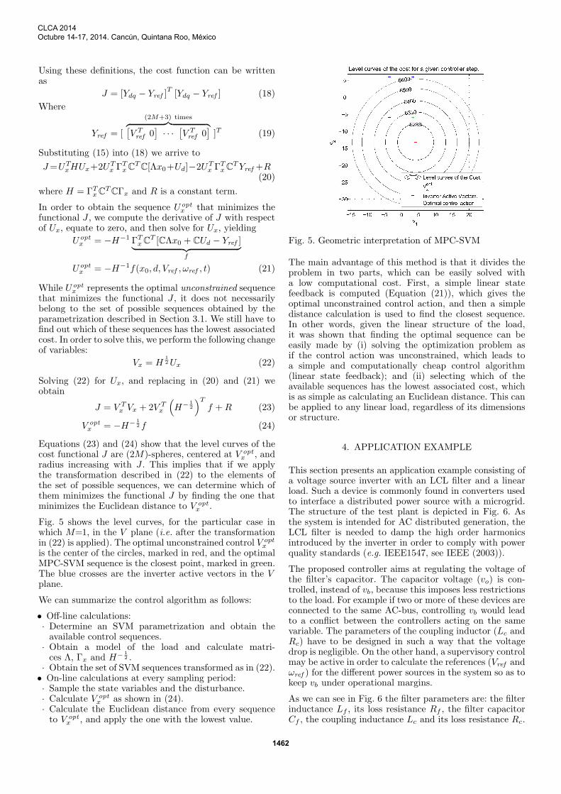
Equations (23) and (24) show that the level curves of thecost functional J are (2M)-spheres, centered at V opt

x , andradius increasing with J . This implies that if we applythe transformation described in (22) to the elements ofthe set of possible sequences, we can determine which ofthem minimizes the functional J by finding the one thatminimizes the Euclidean distance to V opt

x .

Fig. 5 shows the level curves, for the particular case inwhich M=1, in the V plane (i.e. after the transformationin (22) is applied). The optimal unconstrained control V opt

xis the center of the circles, marked in red, and the optimalMPC-SVM sequence is the closest point, marked in green.The blue crosses are the inverter active vectors in the Vplane.

We can summarize the control algorithm as follows:

• Off-line calculations:· Determine an SVM parametrization and obtain theavailable control sequences.

· Obtain a model of the load and calculate matri-ces Λ, Γx and H− 1

2 .· Obtain the set of SVM sequences transformed as in (22).

• On-line calculations at every sampling period:· Sample the state variables and the disturbance.· Calculate V opt

x as shown in (24).· Calculate the Euclidean distance from every sequenceto V opt

x , and apply the one with the lowest value.

Fig. 5. Geometric interpretation of MPC-SVM

The main advantage of this method is that it divides theproblem in two parts, which can be easily solved witha low computational cost. First, a simple linear statefeedback is computed (Equation (21)), which gives theoptimal unconstrained control action, and then a simpledistance calculation is used to find the closest sequence.In other words, given the linear structure of the load,it was shown that finding the optimal sequence can beeasily made by (i) solving the optimization problem asif the control action was unconstrained, which leads toa simple and computationally cheap control algorithm(linear state feedback); and (ii) selecting which of theavailable sequences has the lowest associated cost, whichis as simple as calculating an Euclidean distance. This canbe applied to any linear load, regardless of its dimensionsor structure.

4. APPLICATION EXAMPLE

This section presents an application example consisting ofa voltage source inverter with an LCL filter and a linearload. Such a device is commonly found in converters usedto interface a distributed power source with a microgrid.The structure of the test plant is depicted in Fig. 6. Asthe system is intended for AC distributed generation, theLCL filter is needed to damp the high order harmonicsintroduced by the inverter in order to comply with powerquality standards (e.g. IEEE1547, see IEEE (2003)).

The proposed controller aims at regulating the voltage ofthe filter’s capacitor. The capacitor voltage (vo) is con-trolled, instead of vb, because this imposes less restrictionsto the load. For example if two or more of these devices areconnected to the same AC-bus, controlling vb would leadto a conflict between the controllers acting on the samevariable. The parameters of the coupling inductor (Lc andRc) have to be designed in such a way that the voltagedrop is negligible. On the other hand, a supervisory controlmay be active in order to calculate the references (Vref andωref ) for the different power sources in the system so as tokeep vb under operational margins.

As we can see in Fig. 6 the filter parameters are: the filterinductance Lf , its loss resistance Rf , the filter capacitorCf , the coupling inductance Lc and its loss resistance Rc.

CLCA 2014Octubre 14-17, 2014. Cancún, Quintana Roo, México

1462

Fig. 6. Schematic of the test system.

A state space model of the filter is derived and theobtained structure for the elements in (1) is shownin (25) to (27).The state variables voa, vob represent the‘ab’ components of the capacitor voltage, ila, ilb the filterinductance currents and ioa, iob the coupling inductancecurrents. The input variables of the filter via and vib arethe inverter output voltage components. Finally, vba andvbb are the ‘ab’ components of the voltage at the PCC;as this voltage depends on the dynamics of the load weconsider it as a disturbance to the model.

x = [ila ilb voa vob ioa iob]T (25)

u= [via vib]T d = [vba vbb]

T y = [voa vob]T (26)

A =

−RfLf

I2×2 − 1Lf

I2×2 02×2

1Cf

I2×2 02×2 − 1Cf

I2×2

02×21

LcI2×2 −Rc

LcI2×2

B =

[1

LfI2×2

02×2

02×2

](27)

E =[ 02×2 02×2 − 1Lc

I2×2 ]T

C =[02×2 I2×2 02×2 ]

Table 1. Test System Parameters.

Param. Value Param. Value Param. Value Param. Value

Inverter Parameters

Rf 0.15 Ω Lf 5 mH Cf 65 µF fs 10 KHz

Rc 0.05 Ω Lc 0.53 mH VDC 540 V

Load Parameters References

Rload 25 Ω Lload 1 mH Vref 240 V fref 50 Hz

All the results shown in this section were obtained in sim-ulation. A model of the system in Fig. 6 was implementedin Matlab/Simulink, and as a load ZL we considered alinear RL impedance. For the controller, the sequenceswere divided into 5 subintervals, leading to 91 differentsequences from which to choose the one that minimizesthe cost function. The simulation parameters are listed inTable 1, where fs is the sampling frequency. Fig. 7 showsthe steady state phase voltages at the filter’s capacitor.

In the remainder of this section we analyze both the dy-namic performance of the controller, and the improvementin the calculation time, given by the geometric controller.

4.1 Controller Performance

To obtain a quantity representing the performance ofthe inverter, we calculate the Total Harmonic Distortion(THD) of the output voltage as

%THD = 100(H2

2 +H23 +H2

4 + · · ·+H2∞)/(H2

1

)(28)

where H1 is the RMS value of the fundamental harmonic,and Hn is the RMS values of the n-th harmonic. Thevalue obtained for the steady state phase voltages of theinverter shown in Fig. 7 is THD = 0.44%. This THD valueshows an improvement of the MPC-SVM method over a

classic control scheme characterized by nested PI loopswith SVM modulation proposed, for example, in Huanget al. (2008) which, using the same parameters of Table 1,presents a THD = 1.33%. Fig. 8 compares the outputvoltage (vod and voq) of the proposed controller (MPC-SVM) and the nested PIs structure. It can be seen thatfor the same circuit parameters and inverter frequency theproposed technique shows a sensibly lower ripple.

Fig. 7. Steady state phase voltages of the inverter.

Fig. 8. Output voltage components in steady state, usingdifferent controllers.

4.2 Calculation Improvement

In order to analyze the improvement of the computationaleffort introduced by the geometric implementation, wecalculated at every sampling instant both the geometricand the implicit MPC algorithms; and we stored theamount of time used by each of these procedures for thesame initial conditions. Fig. 9 shows the execution timeof each of the routines for 1000 sampling periods. It isworth mentioning that, as expected, the control actionscalculated by both implementations were the same.

We can observe that the reduction in the computationalcost between the geometric and the implicit versions of thecontrol algorithm is about 80%. The main cause of thisimprovement is that it is not required to perform on-linesimulations of the system response for every possible se-quence. Instead, the calculation of matrices H

12 , Γx and Λ

off-line is required.

CLCA 2014Octubre 14-17, 2014. Cancún, Quintana Roo, México

1463

Fig. 9. Execution time comparison between the Geometricand Implicit implementations of the algorithm.

The obtained reduction in the computational effort, ver-sus the implicit implementation of the algorithm providesthe possibility of increasing the number of subintervalsin a sequence. This would lead to a thinner SVM dis-cretization, thus increasing the available control actions(resulting in the possibility to find sequences closer tothe unconstrained optimal). Note that this improvementin the discretization does not imply an increment in theinverter frequency as the SVM technique is applied in theconstruction of the sequences.

We are currently studying a modification to the presentedmethod to further reduce the computational load. Theobjective is to reduce the number of sequences in thefeasible set where the sequence closest in distance to theunconstrained optimum is selected from. To achieve this,we suggest to calculate the average vector uopt equivalentto the application of the unconstrained optimal sequenceUoptx over a sampling period, that is, if uopt

i are the entriesof Uopt

x , then (with Ti as defined in Appendix A),

uopt = 2(∑M

i=1 Tiuopti

)/Ts = 2Ti

(∑Mi=1 u

opti

)/Ts.

The above vector can be plotted in the (a, b) plane ofFig. 2 to find in which sextant it lies. Then, we can lookfor the closest available sequence only among those whichare synthesized using the two adjacent vectors that limitthe found sextant (and in consequence, result in averagevectors in the same sextant). With the discretizationused in this example, this means calculating 15 distancesinstead of 91. Though we have not implemented thismodification yet, we are confident that the reduction inthe processing time will be sensible. We are currentlyinvestigating the degree of suboptimality (if any) of thissimplified solution.

5. CONCLUSION

A computationally efficient implementation of MPC-SVMcontrol was proposed for three-phase inverters with a linearload. The technique exploits geometric properties of thecost function in order to reduce the calculation’s complex-ity. The obtained implementation avoids the simulationof the system at every sampling instant and for everypossible control sequence by using the associated optimallinear state feedback controller. Then the selection of thesequence with the lowest associated cost is done by findingthe one with the minimum Euclidean distance to theoutput of the state feedback.

The simulation results show an important reduction inthe computational cost of the algorithm, versus the formerimplicit implementation.

REFERENCES

Alvarez Leiva, J.M., Romero, M., and Seron, M. (2013).MPC control for three-phase inverter in stand aloneoperation. In RPIC 2013 - XV Reunion de Trabajo enProcesamiento de la Informacion y Control.

Holmes, D. (1995). The significance of zero spacevector placement for carrier based pwm schemes.In Industry Applications Conference, 1995. ThirtiethIAS Annual Meeting, IAS ’95., Conference Record ofthe 1995 IEEE, volume 3, 2451–2458 vol.3. doi:10.1109/IAS.1995.530615.

Huang, S., Kong, L., Wei, T., and Zhang, G. (2008).Comparative analysis of PI decoupling control strategieswith or without feed-forward in SRF for three-phasepower supply. In International Conference on ElectricalMachines and Systems, 2008. ICEMS 2008, 2372–2377.

IEEE (2003). IEEE standard for interconnect-ing distributed resources with electric powersystems. IEEE Std 1547-2003, 0 1–16. doi:10.1109/IEEESTD.2003.94285.

Lezana, P., Aguilera, R., and Quevedo, D. (2009). Modelpredictive control of an asymmetric flying capacitorconverter. IEEE Transactions on Industrial Electronics,56(6), 1839–1846. doi:10.1109/TIE.2008.2007545.

Rodriguez, J., Pontt, J., Silva, C., Correa, P., Lezana,P., Cortes, P., and Ammann, U. (2007). Predictivecurrent control of a voltage source inverter. IEEETransactions on Industrial Electronics, 54(1), 495–503.doi:10.1109/TIE.2006.888802.

Romero, M., Seron, M., and Goodwin, G. (2011). A com-bined model predictive control/space vector modulation(MPC-SVM) strategy for direct torque and flux controlof induction motors. In IECON 2011 - 37th AnnualConference of the IEEE Industrial Electronics Society,1674–1679. doi:10.1109/IECON.2011.6119558.

Appendix A. MATRIX DEFINITIONS

In the following definitions, T0, T7 and Ti are the durationof the subintervals in which V0, V7 and the remainingvectors in the sequence are applied, respectively. Thesampling time then satisfies: Ts = 2T0 + 2MTi + T7.

A0=eAT0 , As=eATi , A7=eAT7 , Bs=∫ Ti

0eAtBdt, (A.1)

E0=∫ T0

0eAtEdt, Es=

∫ Ti

0eAtEdt, E7=

∫ T7

0eAtEdt

Λ=

λ1

λ2

...λN

, Γx=

γ1,1 γ1,2 ··· γ1,Mγ2,1 γ2,2 γ2,M

.... . .

...γN,1 ··· γN,M

, Γd=

γd1γd2

...γdN

(A.2)

λi=

Ai−1

s A0 if i≤M+1

Ai−M−2s A7A

Ms A0 if M+1<i<2M+3

A0AMs A7A

Ms A0 if i=2M+3

(A.3)

γi,j=

On×2 if i≤j

Ai−j−1s Bs if j<i≤M+1

A7AM−js Bs if i=M+2

Ai−M−2s A7A

M−js Bs+A

i+j−2M−3s Bs if 2M+3−j≤i<2M+3

A0AMs A7A

M−jS

Bs+A0Aj−1s Bs if i=2M+3

Ai−M−2s A7A

M−js Bs Otherwise

(A.4)

γdi=

E0 if i=1

Ai−1s E0+

(∑i−2

l=0Al

s

)Es if 1<i<M+2

A7

[AM

s E0+(∑M−1

l=0Al

s

)Es

]+E7 if i=M+2

Ai−M−2s γd(M+2)+

(∑i−M−3

l=0Al

s

)Es if M+2<i<2M+3

A0

[AM

s γd(M+2)+(∑M−1

l=0Al

s

)Es

]+E0 if i=2M+3

(A.5)

CLCA 2014Octubre 14-17, 2014. Cancún, Quintana Roo, México

1464