geometric methods in vector spaces geometry and meaning

Geometric methods in vector spacesDistributional Semantic Models

Stefan Evert1 & Alessandro Lenci2

1University of Osnabruck, Germany2University of Pisa, Italy

Evert & Lenci (ESSLLI 2009) DSM: Matrix Algebra 30 July 2009 1 / 48

Length & distance Introduction

Geometry and meaning

So far: apply vector methods and matrix algebra to DSMs

Geometric intuition: distance ' semantic (dis)similarityI nearest neighboursI clusteringI semantic mapsI representation for connectionist models

+ We need a mathematical notion of distance!


Length & distance Metric spaces

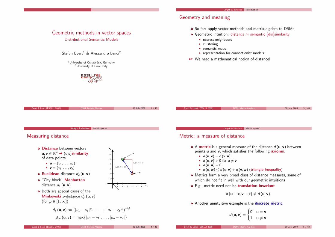
Measuring distance

Distance between vectorsu, v ∈ Rn Ü (dis)similarityof data points

I u = (u1, . . . , un)I v = (v1, . . . , vn)

Euclidean distance d2 (u, v)

“City block” Manhattandistance d1 (u, v)

Both are special cases of theMinkowski p-distance dp (u, v)(for p ∈ [1,∞])

x1

v

x2

1 2 3 4 5

1

2

3

4

5

6

6 u

d2 (!u,!v) = 3.6

d1 (!u,!v) = 5

dp (u, v) :=(|u1 − v1|p + · · ·+ |un − vn|p

)1/p

d∞ (u, v) = max{|u1 − v1|, . . . , |un − vn|

}


Length & distance Metric spaces

Metric: a measure of distance

A metric is a general measure of the distance d (u, v) betweenpoints u and v, which satisfies the following axioms:

I d (u, v) = d (v,u)I d (u, v) > 0 for u 6= vI d (u,u) = 0I d (u,w) ≤ d (u, v) + d (v,w) (triangle inequality)

Metrics form a very broad class of distance measures, some ofwhich do not fit in well with our geometric intuitions

E.g., metric need not be translation-invariant

d (u + x, v + x) 6= d (u, v)

Another unintuitive example is the discrete metric

d (u, v) =

{0 u = v

1 u 6= v


Length & distance Vector norms

Distance vs. norm

Intuitively, distanced (u, v) should correspondto length ‖u− v‖ ofdisplacement vector u− v

I d (u, v) is a metricI ‖u− v‖ is a normI ‖u‖ = d

(u, 0)

Such a metric is alwaystranslation-invariant

dp (u, v) = ‖v − u‖px1

origin

v

x2

1 2 3 4 5

1

2

3

4

5

6

6 u‖!u‖ = d(!u,!0

)

d (!u,!v) = ‖!u − !v‖

‖!v‖ = d(!v,!0

)

Minkowski p-norm for p ∈ [1,∞]:

‖u‖p :=(|u1|p + · · ·+ |un|p

)1/p



Norm: a measure of length

A general norm ‖u‖ for the length of a vector u must satisfythe following axioms:

I ‖u‖ > 0 for u 6= 0I ‖λu‖ = |λ| · ‖u‖ (homogeneity, not req’d for metric)I ‖u + v‖ ≤ ‖u‖ + ‖v‖ (triangle inequality)

every norm defines a translation-invariant metric

d (u, v) := ‖u− v‖



Norm: a measure of length

−1.0 −0.5 0.0 0.5 1.0

−1.

0−

0.5

0.0

0.5

1.0

Unit circle according to p−norm

x1

x 2

p = 1p = 2p = 5p = ∞

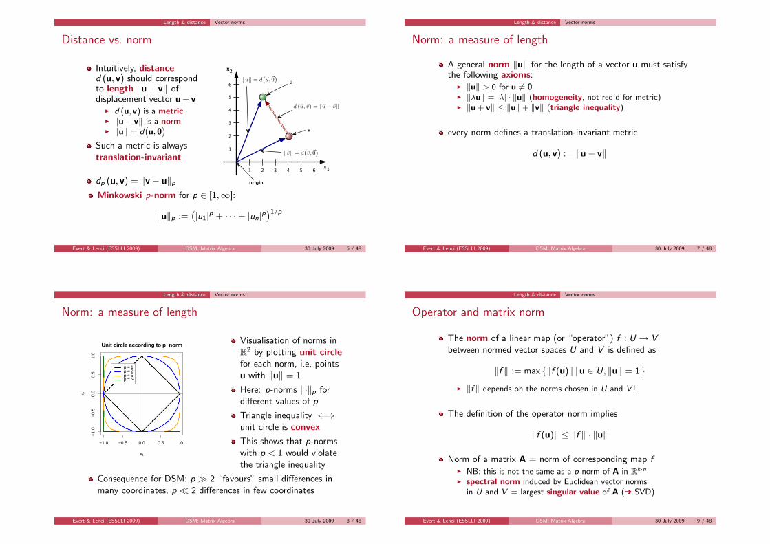
Visualisation of norms inR2 by plotting unit circlefor each norm, i.e. pointsu with ‖u‖ = 1

Here: p-norms ‖·‖p fordifferent values of p

Triangle inequality ⇐⇒unit circle is convex

This shows that p-normswith p < 1 would violatethe triangle inequality

Consequence for DSM: p � 2 “favours” small differences inmany coordinates, p � 2 differences in few coordinates



Operator and matrix norm

The norm of a linear map (or “operator”) f : U → Vbetween normed vector spaces U and V is defined as

‖f ‖ := max {‖f (u)‖ |u ∈ U, ‖u‖ = 1}I ‖f ‖ depends on the norms chosen in U and V !

The definition of the operator norm implies

‖f (u)‖ ≤ ‖f ‖ · ‖u‖

Norm of a matrix A = norm of corresponding map fI NB: this is not the same as a p-norm of A in Rk·n

I spectral norm induced by Euclidean vector normsin U and V = largest singular value of A (Ü SVD)



Which metric should I use?

Choice of metric or norm is one of the parameters of a DSM

Measures of distance between points:I intuitive Euclidean norm ‖·‖2I “city-block” Manhattan distance ‖·‖1I maximum distance ‖·‖∞I general Minkowski p-norm ‖·‖pI and many other formulae . . .

Measures of the similarity of arrows:I “cosine distance” ∼ u1v1 + · · ·+ unvn

I Dice coefficient (matching non-zero coordinates)I and, of course, many other formulae . . .

+ these measures determine angles between arrows

Similarity and distance measures are equivalent!

+ I’m a fan of the Euclidean norm because of its intuitivegeometric properties (angles, orthogonality, shortest path, . . . )


Length & distance with R

Norms & distance measures in R

# We will use the cooccurrence matrix M from the last session> print(M)

eat get hear kill see use

boat 0 59 4 0 39 23

cat 6 52 4 26 58 4

cup 1 98 2 0 14 6

dog 33 115 42 17 83 10

knife 3 51 0 0 20 84

pig 9 12 2 27 17 3

# Note: you can save selected variables with the save() command,# and restore them in your next session (similar to saving R’s workspace)> save(M, O, E, M.mds, file="dsm_lab.RData")

# load() restores the variables under the same names!> load("dsm_lab.RData")




# Define functions for general Minkowski norm and distance;# parameter p is optional and defaults to p = 2> p.norm <- function (x, p=2) (sum(abs(x)^p))^(1/p)> p.dist <- function (x, y, p=2) p.norm(x - y, p)

> round(apply(M, 1, p.norm, p=1), 2)boat cat cup dog knife pig

125 150 121 300 158 70


74.48 82.53 99.20 152.83 100.33 35.44


61.93 66.10 98.01 122.71 86.78 28.31


59 58 98 115 84 27




# Here’s a nice trick to normalise the row vectors quickly> normalise <- function (M, p=2) M / apply(M, 1, p.norm, p=p)

# dist() function also supports Minkowski p-metric# (must normalise rows in order to compare different metrics)> round(dist(normalise(M, p=1), method="minkowski", p=1), 2)

boat cat cup dog knife

cat 0.58

cup 0.69 0.97

dog 0.55 0.45 0.89

knife 0.73 1.01 1.01 1.00

pig 1.03 0.64 1.29 0.71 1.28

# Try different p-norms: how do the distances change?> round(dist(normalise(M, p=2), method="minkowski", p=2), 2)> round(dist(normalise(M, p=4), method="minkowski", p=4), 2)> round(dist(normalise(M, p=99), method="minkowski", p=99), 2)



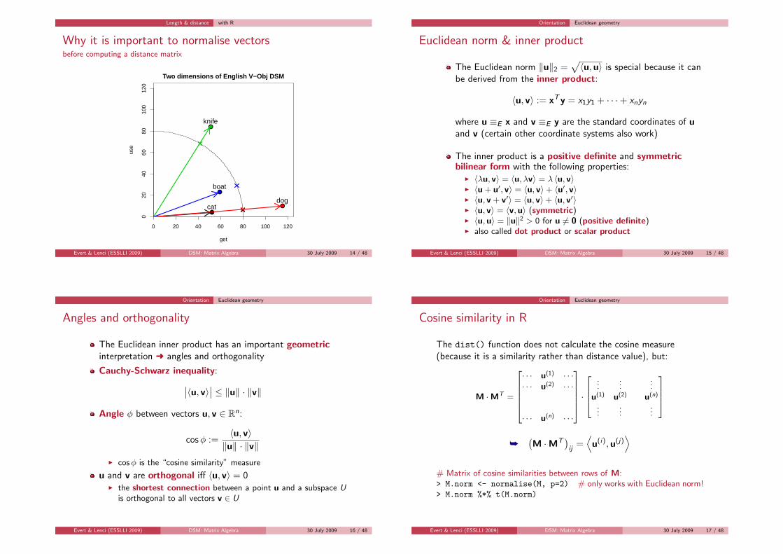
Why it is important to normalise vectorsbefore computing a distance matrix

●

●

●

●

0 20 40 60 80 100 120

020

4060

8010

012

0

Two dimensions of English V−Obj DSM

get

use

catdog

knife

boat


Orientation Euclidean geometry

Euclidean norm & inner product

The Euclidean norm ‖u‖2 =√〈u,u〉 is special because it can

be derived from the inner product:

〈u, v〉 := xT y = x1y1 + · · ·+ xnyn

where u ≡E x and v ≡E y are the standard coordinates of uand v (certain other coordinate systems also work)

The inner product is a positive definite and symmetricbilinear form with the following properties:

I 〈λu, v〉 = 〈u, λv〉 = λ 〈u, v〉I 〈u + u′, v〉 = 〈u, v〉+ 〈u′, v〉I 〈u, v + v′〉 = 〈u, v〉+ 〈u, v′〉I 〈u, v〉 = 〈v,u〉 (symmetric)I 〈u,u〉 = ‖u‖2 > 0 for u 6= 0 (positive definite)I also called dot product or scalar product



Angles and orthogonality

The Euclidean inner product has an important geometricinterpretation Ü angles and orthogonality

Cauchy-Schwarz inequality:

∣∣〈u, v〉∣∣ ≤ ‖u‖ · ‖v‖

Angle φ between vectors u, v ∈ Rn:

cosφ :=〈u, v〉‖u‖ · ‖v‖

I cosφ is the “cosine similarity” measure

u and v are orthogonal iff 〈u, v〉 = 0I the shortest connection between a point u and a subspace U

is orthogonal to all vectors v ∈ U



Cosine similarity in R

The dist() function does not calculate the cosine measure(because it is a similarity rather than distance value), but:

M ·MT =

· · · u(1) · · ·· · · u(2) · · ·

· · · u(n) · · ·

·

......

...u(1) u(2) u(n)

......

...

å(M ·MT

)ij

=⟨

u(i),u(j)⟩

# Matrix of cosine similarities between rows of M:> M.norm <- normalise(M, p=2) # only works with Euclidean norm!> M.norm %*% t(M.norm)



Euclidean distance or cosine similarity?

Which is better, Euclidean distance or cosine similarity?

They are equivalent: if vectors are normalised (‖u‖2 = 1),both lead to the same neighbour ranking

d2 (u, v) =√‖u− v‖2 =

√〈u− v,u− v〉

=√〈u,u〉+ 〈v, v〉 − 2 〈u, v〉

=√‖u‖2 + ‖v‖2 − 2 〈u, v〉

=√

2− 2 cosφ



Euclidean distance and cosine similarity

●

●

●

●

0 20 40 60 80 100 120

020

4060

8010

012

0

Two dimensions of English V−Obj DSM

get

use

catdog

knife

boat

αα



Cartesian coordinates

A set of vectors b(1), . . . ,b(n) is called orthonormal if thevectors are pairwise orthogonal and of unit length:

I⟨b(j),b(k)

⟩= 0 for j 6= k

I⟨b(k),b(k)

⟩=∥∥b(k)

∥∥2= 1

An orthonormal basis and the corresponding coordinates arecalled Cartesian

Cartesian coordinates are particularly intuitive, and the innerproduct has the same form wrt. every Cartesian basis B: foru ≡B x′ and v ≡B y′, we have

〈u, v〉 = (x′)T y′ = x ′1y′1 + · · ·+ x ′ny

′n

NB: the column vectors of the matrix B are orthonormalI recall that the columns of B specify the standard coordinates

of the vectors b(1), . . . ,b(n)



Orthogonal projection

Cartesian coordinates u ≡B x can easily be computed:

⟨u,b(k)

⟩=

⟨n∑

j=1

xjb(j),b(k)

⟩

=n∑

j=1

xj

⟨b(j),b(k)

⟩

︸︷︷︸=δjk

= xk

I Kronecker delta: δjk = 1 for j = k and 0 for j 6= k

Orthogonal projection PV : Rn → V to subspaceV := sp

(b(1), . . . ,b(k)

)(for k < n) is given by

PV u :=k∑

j=1

b(j)⟨

u,b(j)⟩


Orientation Normal vector

Hyperplanes & normal vectorsA hyperplane is the decision boundary of a linear classifier!

A hyperplane U ⊆ Rn through the origin 0 can becharacterized by the equation

U ={

u ∈ Rn∣∣ 〈u,n〉 = 0

}

for a suitable n ∈ Rn with ‖n‖ = 1

n is called the normal vector of U

The orthogonal projection PU into U is given by

PUv := v − n 〈v,n〉An arbitrary hyperplane Γ ⊆ Rn can analogously becharacterized by

Γ ={

u ∈ Rn∣∣ 〈u,n〉 = a

}

where a ∈ R is the (signed) distance of Γ from 0


Orientation Isometric maps

Orthogonal matrices

A matrix A whose column vectors are orthonormal is calledan orthogonal matrix

AT is orthogonal iff A is orthogonal

The inverse of an orthogonal matrix is simply its transpose:

A−1 = AT if A is orthogonal

I it is easy to show AT A = I by matrix multiplication,since the columns of A are orthonormal

I since AT is also orthogonal, it follows thatAAT = (AT )T AT = I

I side remark: the transposition operator ·T is calledan involution because (AT )T = A



Isometric maps

An endomorphism f : Rn → Rn is called an isometry iff〈f (u), f (v)〉 = 〈u, v〉 for all u, v ∈ Rn

Geometric interpretation: isometries preserve angles anddistances (which are defined in terms of 〈·, ·〉)f is an isometry iff its matrix A is orthogonal

Coordinate transformations between Cartesian systems areisometric (because B and B−1 = BT are orthogonal)

Every isometric endomorphism of Rn can be written as acombination of planar rotations and axial reflections in asuitable Cartesian coordinate system

R(1,3)φ =

[cos φ 0 − sin φ

0 1 0sin φ 0 cos φ

], Q(2) =

[1 0 00 −1 00 0 1

]



Summary: orthogonal matrices

The column vectors of an orthogonal n × n matrix B form aCartesian basis b(1), . . . ,b(n) of Rn

B−1 = BT , i.e. we have BT B = BBT = I

The coordinate transformation BT into B-coordinates is anisometry, i.e. all distances and angles are preserved

The first k < n columns of B form a Cartesian basis of asubspace V = sp

(b(1), . . . ,b(k)

)of Rn

The corresponding rectangular matrix B =[b(1), . . . ,b(k)

]

performs an orthogonal projection into V :

PV u ≡B BT x (for u ≡E x)

≡E BBT x

å These properties will become important later today!


Orientation General inner product

General inner products

Can we also introduce geometric notions such as angles andorthogonality for other metrics, e.g. the Manhattan distance?

+ norm must be derived from appropriate inner product

General inner products are defined by

〈u, v〉B := (x′)T y′ = x ′1y′1 + · · ·+ x ′yy ′n

wrt. non-Cartesian basis B (u ≡B x′, v ≡B y′)

〈·, ·〉B can be expressed in standard coordinates u ≡E x,v ≡E y using the transformation matrix B:

〈u, v〉B = (x′)T y′ =(B−1x

)T (B−1y

)

= xT (B−1)T B−1y =: xT Cy




The coefficient matrix C := (B−1)T B−1 of the general innerproduct is symmetric

CT = (B−1)T ((B−1)T )T = (B−1)T B−1 = C

and positive definite

xT Cx =(B−1x

)T (B−1x

)= (x′)T x′ ≥ 0

It is (relatively) easy to show that every positive definite andsymmetric bilinear form can be written in this way.

+ i.e. every norm that is derived from an inner product can beexpressed in terms of a coefficient matrix C or basis B




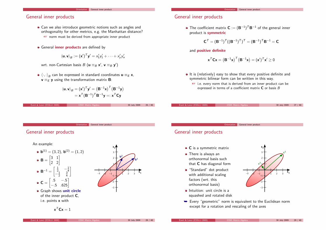
An example:

b(1) = (3, 2), b(2) = (1, 2)

B =

[3 12 2

]

B−1 =

[12 −1

4−1

234

]

C =

[.5 −.5−.5 .625

]

Graph shows unit circleof the inner product C,i.e. points x with

xT Cx = 1

x1

x2

-3 -2 -1 1 2

-3

-2

-1

1

2

3

3

b1b2




C is a symmetric matrix

There is always anorthonormal basis suchthat C has diagonal form

“Standard” dot productwith additional scalingfactors (wrt. thisorthonormal basis)

Intuition: unit circle is asquashed and rotated disk

x1

x2

-3 -2 -1 1 2

-3

-2

-1

1

2

3

3

c2

c1

å Every “geometric” norm is equivalent to the Euclidean normexcept for a rotation and rescaling of the axes


PCA Motivation and example data

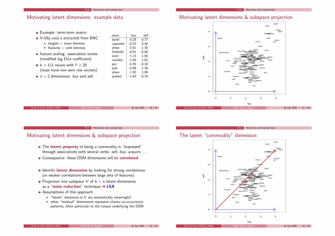
Motivating latent dimensions: example data

Example: term-term matrix

V-Obj cooc’s extracted from BNCI targets = noun lemmasI features = verb lemmas

feature scaling: association scores(modified log Dice coefficient)

k = 111 nouns with f ≥ 20(must have non-zero row vectors)

n = 2 dimensions: buy and sell

noun buy sell

bond 0.28 0.77cigarette -0.52 0.44dress 0.51 -1.30freehold -0.01 -0.08land 1.13 1.54number -1.05 -1.02per -0.35 -0.16pub -0.08 -1.30share 1.92 1.99system -1.63 -0.70



Motivating latent dimensions & subspace projection

0 1 2 3 4

01

23

4

buy

sell

acre

advertising

amount

arm

asset

bag

beerbill

bit

bond book

bottle

boxbread

building

business

car

card

carpet

cigaretteclothe

club

coal

collectioncompany

computer

copy

couple

currency

dress

drink

drugequipmentestate

farm

fish

flat

flower

foodfreehold

fruitfurniture

good

home

horse

house

insurance

item

kind

land

licence

liquor

lotmachine

material

meat milkmill

newspaper

number

oil

one

packpackagepacket

painting

pair

paperpart

per

petrol

picture

piece

place

plant

player

pound

productproperty

pub

quality

quantity

range

record

right

seatsecurity

service

set

share

shoe

shop

sitesoftware

stake

stamp

stock

stuff

suit

system

television

thing

ticket

time

tin

unit

vehicle

video

wine

work

year



Motivating latent dimensions & subspace projection

The latent property of being a commodity is “expressed”through associations with several verbs: sell, buy, acquire, . . .

Consequence: these DSM dimensions will be correlated

Identify latent dimension by looking for strong correlations(or weaker correlations between large sets of features)

Projection into subspace V of k < n latent dimensionsas a “noise reduction” technique Ü LSA

Assumptions of this approach:I “latent” distances in V are semantically meaningfulI other “residual” dimensions represent chance co-occurrence

patterns, often particular to the corpus underlying the DSM



The latent “commodity” dimension

0 1 2 3 4

01

23

4

buy

sell

acre

advertising

amount

arm

asset

bag

beerbill

bit

bond book

bottle

boxbread

building

business

car

card

carpet

cigaretteclothe

club

coal

collectioncompany

computer

copy

couple

currency

dress

drink

drugequipmentestate

farm

fish

flat

flower

foodfreehold

fruitfurniture

good

home

horse

house

insurance

item

kind

land

licence

liquor

lotmachine

material

meat milkmill

newspaper

number

oil

one

packpackagepacket

painting

pair

paperpart

per

petrol

picture

piece

place

plant

player

pound

productproperty

pub

quality

quantity

range

record

right

seatsecurity

service

set

share

shoe

shop

sitesoftware

stake

stamp

stock

stuff

suit

system

television

thing

ticket

time

tin

unit

vehicle

video

wine

work

year


PCA Calculating variance

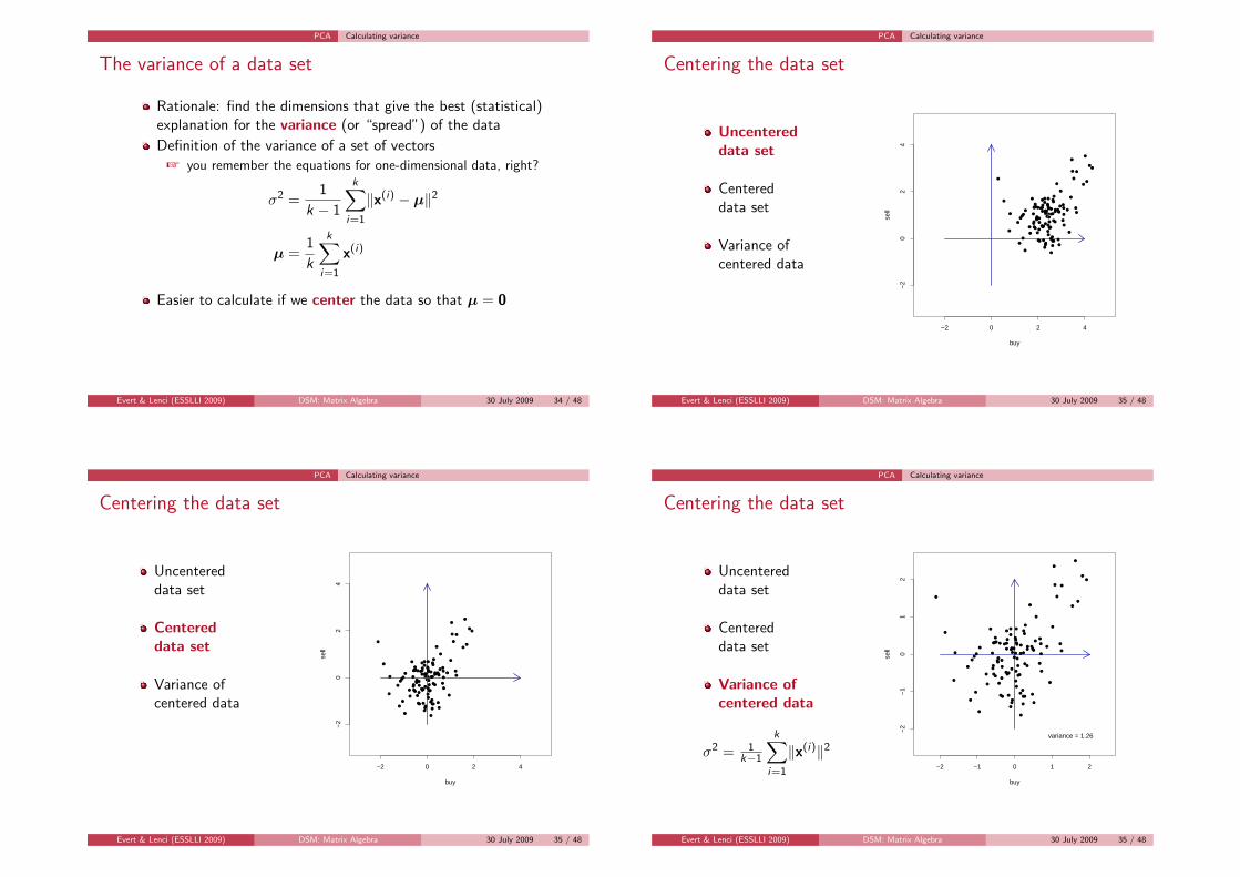
The variance of a data set

Rationale: find the dimensions that give the best (statistical)explanation for the variance (or “spread”) of the data

Definition of the variance of a set of vectors

+ you remember the equations for one-dimensional data, right?

σ2 =1

k − 1

k∑

i=1

‖x(i) − µ‖2

µ =1

k

k∑

i=1

x(i)

Easier to calculate if we center the data so that µ = 0



Centering the data set

Uncentereddata set

Centereddata set

Variance ofcentered data

σ2 = 1k−1

k∑

i=1

‖x(i)‖2

−2 0 2 4

−2

02

4

buy

sell

●

●

●

●

●

●

●

●

●

● ●

●

●●

●

●

●

●

●

●

●

●

●

●●

●

●

●

●

●

●

●●●

●

●

●

●

●

●

●●

●

●

●

●

●

●

●

●

●

●

●

●

●

● ●●

●

●

●

●

● ●●

●

●

●●

●

●

●

●

●

●

●

●

● ●

●

●

●

●

●

●

●●

●

●

●

●

●

●●

●

●

●

●

●

●

●

●

●

●

●

●

●

●

●

●

●




Uncentereddata set

Centereddata set


σ2 = 1k−1

k∑

i=1

‖x(i)‖2

−2 0 2 4

−2

02

4

buy

sell

●

●

●

●

●

●

●

●

●

● ●

●

●●

●

●

●

●

●

●

●

●

●

●●

●

●

●

●

●

●

●●●

●

●

●

●

●

●

●●

●

●

●

●

●

●

●

●

●

●

●

●

●

● ●●

●

●

●

●

● ●●

●

●

●●

●

●

●

●

●

●

●

●

● ●

●

●

●

●

●

●

●●

●

●

●

●

●

●●

●

●

●

●

●

●

●

●

●

●

●

●

●

●

●

●

●




Uncentereddata set

Centereddata set


σ2 = 1k−1

k∑

i=1

‖x(i)‖2−2 −1 0 1 2

−2

−1

01

2

buy

sell

●

●

●

●

●

●

●

●

●

●●

●

●●

●

●

●

●

●

●

●

●

●

●

●

●

●

●

●

●

●

●

●●

●

●

●

●

●

●

●●

●

●

●

●

●

●

●

●

●

●

●

●

●

●●

●

●

●

●

●

● ●

●

●

●

●●

●

●

●

●

●

●

●

●

● ●

●

●

●

●

●

●

●

●

●

●

●

●

●

●●

●

●

●

●

●

●

●

●

●

●

●

●

●

●

●

●

●

variance = 1.26


PCA Projection

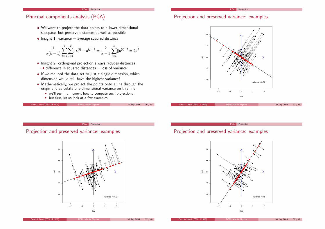
Principal components analysis (PCA)

We want to project the data points to a lower-dimensionalsubspace, but preserve distances as well as possible

Insight 1: variance = average squared distance

1

k(k − 1)

k∑

i=1

k∑

j=1

‖x(i) − x(j)‖2 =2

k − 1

k∑

i=1

‖x(i)‖2 = 2σ2

Insight 2: orthogonal projection always reduces distancesÜ difference in squared distances = loss of variance

If we reduced the data set to just a single dimension, whichdimension would still have the highest variance?

Mathematically, we project the points onto a line through theorigin and calculate one-dimensional variance on this line

I we’ll see in a moment how to compute such projectionsI but first, let us look at a few examples


PCA Projection

Projection and preserved variance: examples

−2 −1 0 1 2

−2

−1

01

2

buy

sell

●

●

●

●

●

●

●

●

●

●●

●

●●

●

●

●

●

●

●

●

●

●

●

●

●

●

●

●

●

●

●

●●

●

●

●

●

●

●

●●

●

●

●

●

●

●

●

●

●

●

●

●

●

●●

●

●

●

●

●

● ●

●

●

●

●●

●

●

●

●

●

●

●

●

● ●

●

●

●

●

●

●

●

●

●

●

●

●

●

●●

●

●

●

●

●

●

●

●

●

●

●

●

●

●

●

●

●

●

●

●

●

●

●

●

●

●●

●

●●●

●

●

●

●

●

●

●

●

●

●

●

●

●

●

●

●

●

●

●

●

●

●

●

●

●

●

●●●

●●

●

●

●

●

●

●

●

●

●

●

●

●

●

●●

●

●

●

●

●

●

●

●

●

●

●●

●

●

●●

●

●

●

●

●

●

●

●

●

●

●

●

●

●

●

●●

●

●

●

●

●

●

●

●

●●

●●

●●

●

●

●

●

variance = 0.36


PCA Projection


−2 −1 0 1 2

−2

−1

01

2

buy

sell

●

●

●

●

●

●

●

●

●

●●

●

●●

●

●

●

●

●

●

●

●

●

●

●

●

●

●

●

●

●

●

●●

●

●

●

●

●

●

●●

●

●

●

●

●

●

●

●

●

●

●

●

●

●●

●

●

●

●

●

● ●

●

●

●

●●

●

●

●

●

●

●

●

●

● ●

●

●

●

●

●

●

●

●

●

●

●

●

●

●●

●

●

●

●

●

●

●

●

●

●

●

●

●

●

●

●

●

●

●

●

●

●

●

●

●

●

●

●

●

● ●

●

●

●

●● ●

●

●●

●

●

●

●

●

●

●

●

●

●

●●●●

●

●

●●●

●

●

●

●

●

●

●

●

●

●

●

●

●●

●

●●

●

●

●

●

●

●

●

●

●

●

●●

●●

●●

●

●

●●

●●

●

●

●

●

●

●●

●

●

●

●

●

●

●

●

●●

●

●

●

●

●

●

●

●

●

●●

●

●

variance = 0.72


PCA Projection


−2 −1 0 1 2−

2−

10

12

buy

sell

●

●

●

●

●

●

●

●

●

●●

●

●●

●

●

●

●

●

●

●

●

●

●

●

●

●

●

●

●

●

●

●●

●

●

●

●

●

●

●●

●

●

●

●

●

●

●

●

●

●

●

●

●

●●

●

●

●

●

●

● ●

●

●

●

●●

●

●

●

●

●

●

●

●

● ●

●

●

●

●

●

●

●

●

●

●

●

●

●

●●

●

●

●

●

●

●

●

●

●

●

●

●

●

●

●

●

●

●

●

●●

●

●

●●

●

●

●

●

●●

●

●

●

●

●

●

●

●

●

●

●

●

●

●

●

●

●

●

●

●

●

●

●

●

●

●

●●

●

●

●

●

●

●

●

●

●

●

●

●

●

●

●

●

●

●

●

●●

●

●

●

●●

●

●

●

●

●

●

●

●

●

●●

●

●

●

●

●

●

●

●

●

●

●

●

●

●

●

●

●

●

●

●

●

●

●

●

●

●

●

●●●

●

●

variance = 0.9


PCA Projection

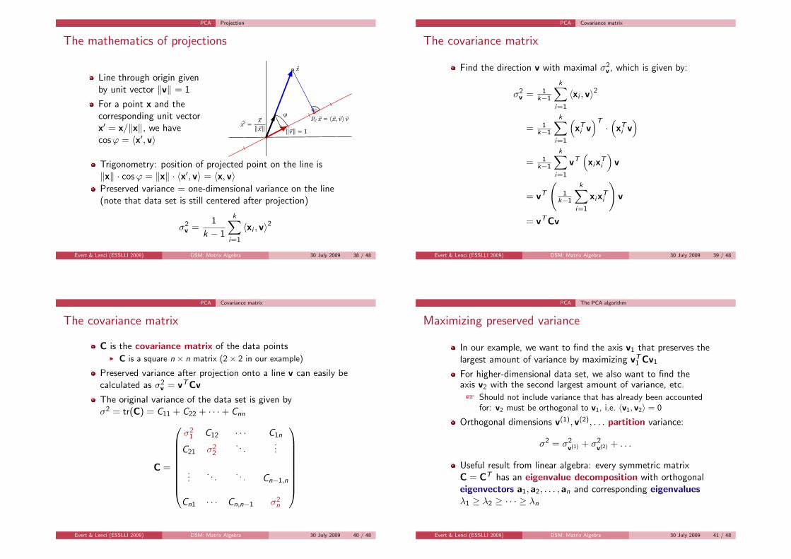
The mathematics of projections

Line through origin givenby unit vector ‖v‖ = 1

For a point x and thecorresponding unit vectorx′ = x/‖x‖, we havecosϕ = 〈x′, v〉

.ϕ

‖!v‖ = 1

!x

!x′ =!x

‖!x‖P!v !x = 〈!x, !v〉 !v

Trigonometry: position of projected point on the line is‖x‖ · cosϕ = ‖x‖ · 〈x′, v〉 = 〈x, v〉Preserved variance = one-dimensional variance on the line(note that data set is still centered after projection)

σ2v =

1

k − 1

k∑

i=1

〈xi , v〉2


PCA Covariance matrix

The covariance matrix

Find the direction v with maximal σ2v , which is given by:

σ2v = 1

k−1

k∑

i=1

〈xi , v〉2

= 1k−1

k∑

i=1

(xTi v)T·(

xTi v)

= 1k−1

k∑

i=1

vT(

xixTi

)v

= vT

(1

k−1

k∑

i=1

xixTi

)v

= vT Cv


PCA Covariance matrix

The covariance matrix

C is the covariance matrix of the data pointsI C is a square n × n matrix (2× 2 in our example)

Preserved variance after projection onto a line v can easily becalculated as σ2

v = vT Cv

The original variance of the data set is given byσ2 = tr(C) = C11 + C22 + · · ·+ Cnn

C =

σ21 C12 · · · C1n

C21 σ22

. . ....

.... . .

. . . Cn−1,n

Cn1 · · · Cn,n−1 σ2n


PCA The PCA algorithm

Maximizing preserved variance

In our example, we want to find the axis v1 that preserves thelargest amount of variance by maximizing vT

1 Cv1

For higher-dimensional data set, we also want to find theaxis v2 with the second largest amount of variance, etc.

+ Should not include variance that has already been accountedfor: v2 must be orthogonal to v1, i.e. 〈v1, v2〉 = 0

Orthogonal dimensions v(1), v(2), . . . partition variance:

σ2 = σ2v(1) + σ2

v(2) + . . .

Useful result from linear algebra: every symmetric matrixC = CT has an eigenvalue decomposition with orthogonaleigenvectors a1, a2, . . . , an and corresponding eigenvaluesλ1 ≥ λ2 ≥ · · · ≥ λn



Eigenvalue decomposition

The eigenvalue decomposition of C can be written in the form

C = U ·D ·UT

where U is an orthogonal matrix of eigenvectors (columns)and D = Diag(λ1, . . . , λn) a diagonal matrix of eigenvalues

U =

......

......

......

a1 a2 · · · an

......

......

......

D =

λ1

λ2

. . .. . .

λn

I note that both U and D are n × n square matrices



The PCA algorithm

With the eigenvalue decomposition of C, we have

σ2v = vT Cv = vT UDUT v = (UT v)T D(UT v) = yT Dy

where y = UT v = [y1, y2, . . . , yn]T are the coordinates of v inthe Cartesian basis formed by the eigenvectors of C

‖y‖ = 1 since UT is an isometry (orthogonal matrix)

We therefore want to maximize

vT Cv = λ1(y1)2 + λ2(y2)2 · · ·+ λn(yn)2

under the constraint (y1)2 + (y2)2 + · · ·+ (yn)2 = 1

Solution: y = [1, 0, . . . , 0]T (since λ1 is the largest eigenvalue)

This corresponds to v = a1 (the first eigenvector of C) and apreserved amount of variance given by σ2

v = aT1 Ca1 = λ1



The PCA algorithm

In order to find the dimension of second highest variance,we have to look for an axis v orthogonal to a1

+ UT is orthogonal, so the coordinates y = UT v must beorthogonal to first axis [1, 0, . . . , 0]T , i.e. y = [0, y2, . . . , yn]T

In other words, we have to maximize

vT Cv = λ2(y2)2 · · ·+ λn(yn)2

under constraints y1 = 0 and (y2)2 + · · ·+ (yn)2 = 1

Again, solution is y = [0, 1, 0, . . . , 0]T , corresponding to thesecond eigenvector v = a2 and preserved variance σ2

v = λ2

Similarly for the third, fourth, . . . axis



The PCA algorithm

The eigenvectors ai of the covariance matrix C are called theprincipal components of the data set

The amount of variance preserved (or “explained”) by the i-thprincipal component is given by the eigenvalue λi

Since λ1 ≥ λ2 ≥ · · · ≥ λn, the first principal componentaccounts for the largest amount of variance etc.

Coordinates of a point x in PCA space are given by UT x(note: these are the projections on the principal components)

For the purpose of “noise reduction”, only the first n′ < nprincipal components (with highest variance) are retained, andthe other dimensions in PCA space are dropped

+ i.e. data points are projected into the subspace V spanned bythe first n′ column vectors of U



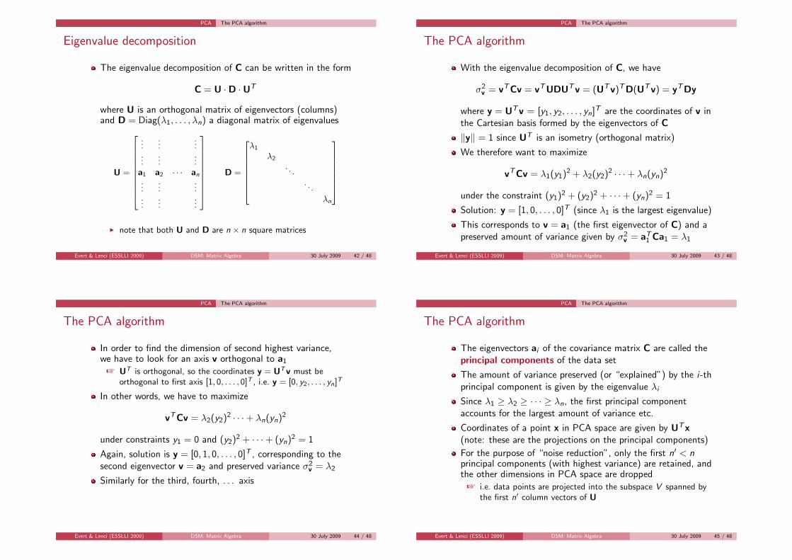
PCA example

−2 −1 0 1 2

−2

−1

01

2

buy

sell

●

●

●

●

●

●

●

●

●

●●

●

●●

●

●

●

●

●

●

●

●

●

●

●

●

●

●

●

●

●

●

●●

●

●

●

●

●

●

●●

●

●

●

●

●

●

●

●

●

●

●

●

●

●●

●

●

●

●

●

● ●

●

●

●

●●

●

●

●

●

●

●

●

●

● ●

●

●

●

●

●

●

●

●

●

●

●

●

●

●●

●

●

●

●

●

●

●

●

●

●

●

●

●

●

●

●

●

●

●

●

●

●

●

●

●

●

●

●

●

●

●

●●

●●

●

●

●

●

● ●

●

●

●

●

●

●

●

book

bottle

good

house

packetpart

stock

system

advertising

arm

asset

car

clothecollection

copy

dress

food

insurance

land

liquor

number one pairpound

product

propertyshare

suit

ticket

time

year


PCA with R

PCA in R

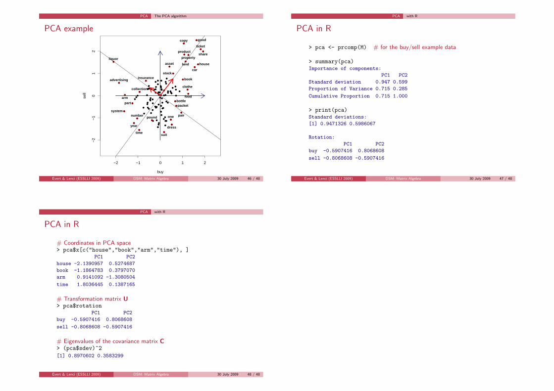
> pca <- prcomp(M) # for the buy/sell example data

> summary(pca)Importance of components:

PC1 PC2

Standard deviation 0.947 0.599

Proportion of Variance 0.715 0.285

Cumulative Proportion 0.715 1.000

> print(pca)Standard deviations:

[1] 0.9471326 0.5986067

Rotation:

PC1 PC2

buy -0.5907416 0.8068608

sell -0.8068608 -0.5907416


PCA with R

PCA in R

# Coordinates in PCA space> pca$x[c("house","book","arm","time"), ]

PC1 PC2

house -2.1390957 0.5274687

book -1.1864783 0.3797070

arm 0.9141092 -1.3080504

time 1.8036445 0.1387165

# Transformation matrix U> pca$rotation

PC1 PC2

buy -0.5907416 0.8068608

sell -0.8068608 -0.5907416

# Eigenvalues of the covariance matrix C> (pca$sdev)^2[1] 0.8970602 0.3583299


geometric methods in vector spaces geometry and meaning

Documents