GEOMETRIC MAGIC SQUARESA Challenging New Twist Using Colored Shapes

Instead of Numbers

LEE C. F. SALLOWS

DOVER PUBLICATIONS, INC.Mineola, New York

2

CopyrightCopyright © 2013 by Lee C. F. Sallows

All rights reserved.

Bibliographical NoteGeometric Magic Squares is a new work,

first published by Dover Publications, Inc., in 2013.

International Standard Book NumbereISBN-13: 978-0-486-29002-7

Manufactured in the United States by Courier Corporation48909401

www.doverpublications.com

3

Contents

Foreword

Part I: Geomagic Squares of 3×31. Introduction2. Geometric Magic Squares3. The Five Types of 3×3 Area Square4. Construction by Formula5. Construction by Computer6. 3×3 Squares7. 3×3 Nasiks and Semi-Nasiks8. Special Examples of 3×3 Squares

Part II: Geomagic Squares of 4×49. Geo-Latin Squares

10. 4×4 Nasiks11. Graeco-Latin Templates12. Uniform Square Substrates13. Dudeney’s 12 Graphic Types14. The 12 Formulae15. A Type I Geomagic Square16. Self-Interlocking Geomagics17. Form and Emptiness18. Further Variations

Part III: Special Categories19. 2×2 Squares20. Picture-Preserving Geomagics21. 3-Dimensional Geomagics22. Alpha-Geomagic Squares23. Normal Squares of Order-424. Eccentric Squares25. Collinear Collations26. Concluding Remarks

Appendix I. A Formal Definition of Geomagic SquaresAppendix II. Magic FormulaeAppendix III. New Advances with 4×4 Magic SquaresAppendix IV. The Dual of the Lo shuAppendix V. The Lost Theorem

GlossaryReferences

4

For Evie,Alright Rat?

Note: The numbers in square brackets in the text refer to the References at the end of the book.

5

Foreword

It is now almost forty years since a rainy afternoon in Nijmegen when I found that afit of absent-minded doodling had inadvertantly developed into an attempt toconstruct a magic square. I was twenty-six at the time, a Brit recently arrived inHolland, where I was destined to remain domiciled down to the present day.Nijmegen is a town on the eastern side of the Netherlands, not far from Arnhem,close to the border with Germany. The reasons that had brought me to Nijmegenmight be of interest in a different context, but are of no relevance to the presentaccount. Like the First Patriarch of Zen Buddhism, I had just blown in from theWest. The year was 1970, and I had landed a job as an electronics engineer at thelocal university, getting in via the back door as a member of their non-academicstaff. The lab was new and set amid woodland. Compared to the workingconditions I’d known back home, this was paradise. Also, the technical equipmentavailable in the department was years ahead of anything I’d seen in England.Moreover, my income had doubled. Small wonder then that I stayed, although littledid I then realize that it would be for life.

I cannot now even recall how or where I had first learned what a magic squareis. The most probable source would have been one of the comics I read as a boygrowing up in London, most likely my favourite, The Eagle, which enlivened itspages with verbal and mathematical curiosities, and had introduced me to my firstpalindrome, “Evil rats on no star live.” A palindrome is a sentence that reads thesame backwards as it does forwards. My own name can be appended backwards toitself to produce the almost-palindrome, “Lee Sallows swollas eel.” If you likepalindromes then there is a good chance you will like magic squares too. It is athirst for symmetry shared by many. In any case, the concept of a magic square hadsomehow lodged in my mind, so that the purpose guiding my doodling hand allthose years later was at least clear. It was to arrange the numbers from 1 to 9 in asquare grid of nine cells so that the sum of any three of them lying in a straight linewould be the same. Eight such straight-line-triplets can be traced in a square ofnine cells, three of them forming its rows, three its columns, and two its corner-to-corner diagonals. Warming to my task, it seemed to me sufficiently wonderful thatnine numbers could be found to realize the desired result at all, let alone that itcould be achieved using the natural numbers from one to nine. However, I couldclearly remember having seen such a square somewhere before, so there was nodoubt in my mind that it could be done. In fact, the puzzle presents little difficulty,and within a few minutes I was able to examine my solution at leisure. It can be

6

seen in Figure 1.1 of the Introduction, the very first illustration in this book.To the receptive eye there is something deeply satisfying in such a square. See,

for example, how the four pairs straddling the centre number each sum to ten. Thereare just four possible ways to split ten into two distinct whole numbers, and all ofthem appear here. Similarly, there are just eight possible ways in which threedifferent decimal digits can combine to yield 15. Again, every one of them is to befound occupying a row, column, or diagonal in the magic square.

In my mind’s eye, I imagined the numbers replaced by weights of 1, 2, 3,…,standing on a square board at nine spots corresponding to the exact centre of eachcell in the 3×3 grid. Ideally, these weights would all be of the same size and shape.Underneath the board, at its exact centre, was a pivot. And upon this pivot theboard would perch in perfect balance, a reflection of the numerical balancerealized in the magic square. Years later I saw a photograph of an almost identicalconstruction due to Craig Knecht, only with the board suspended from its centre bya wire, instead of balanced on a pivot1. Craig had the clever idea of building hisweights from different numbers of identical metal rings, or washers, piled atopeach other on vertical posts that stuck upwards from the centre of every squarecell.

But back to that rainy day in Nijmegen. Re-examining my new plaything,questions began to form. Could a second magic square be produced by arrangingthe same numbers differently? What of alternative numbers? Simple and pleasingas are 1,2,3, … , clearly others might be used to similar effect. Then again, werelarger magic squares to be found? Could the numbers from 1 to 16 be used toproduce a 4×4 specimen? Let’s see, supposing we call the number in the top left-hand cell … I had no training in mathematics, but I found myself trying to recallsome of the half-forgotten algebra learned at school. Little did I know it, but I wasplaying with fire. There are some people for whom magic squares are moreaddictive than cocaine. I should know; here I am forty years later and still hooked.

It was soon after this that I first ran across Martin Gardner’s “MathematicalGames” column in Scientific American, and was thus introduced to the world ofrecreational mathematics. With his genius for making difficult things easy, Gardnerled me into that world until I felt confident enough to start making my own way.There was no Internet in those days. It was only through Martin Gardner’s writingsthat I became aware of the extensive literature on magic squares, a literature that Inow began to explore. However, beyond this there were the rows of boundvolumes of Scientific American I found lining the shelves of our university library.The series went back some twenty-five years, and every single issue contained anas-yet-to-be-read Mathematical Games column. It took me a around a month towork through the entire series, an exercise from which I emerged with more or less

7

glazed eyes and a burning desire to contribute to the field something new of myown. Gardner had woken me up to the fact that many of the ideas and inventionsfound in Mathematical Games were the products of amateurs; that you didn’t needa diploma to do your own research, that permission is not required before making anew discovery.

It was, in fact, in the field of magic squares that I landed my first ever new‘find,’ which was an improved algebraic generalization of 4×4 squares. A triflinginnovation, it was nonetheless poignant for me in showing that it was indeedpossible for a rank amateur to make an original discovery, an insight from which Inever looked back. Thus, while no mathematical mountaineer, I set out on my ownto explore low-level routes, discovering in the process a great liking formathematical wordplay. It was in this way that what had become a compulsivehabit of playing with words and numbers lead eventually to the idea of‘alphamagic’ squares, a frivolous invention that has come to enjoy a modestrenown. Some examples can be found in this volume. Still, later, these werefollowed by two more novelties in the shape of ‘septivigesimal’ magic squares and‘ambimagic’ squares. Septivigesimal is just a long word for “twenty-seven-based.”It refers to a certain gematria or system for interpreting words as numbers. Themagic squares referred to are ones in which words occupy the cells, their values,as interpreted in the gematria, then emerging as numbers that form a conventionalmagic square. Ambimagic squares come up for brief elucidation in Part II of thisbook. Of course, magic squares were only one among other topics in recreationalmath to attract my interest. But that they have loomed large in my thoughts over along period of years cannot be denied.

I first hit on the idea of a geometric magic square in October 2001, and I sensedat once that I had penetrated some previously hidden portal and was now standingon the threshold of a great adventure. It was going to be like exploring Aladdin’sCave. That there were treasures in the cave, I was convinced, but how they were tobe found was far from clear. The concept of a geometric magic square is so simplethat a child will grasp it in a single glance. Ask a mathematician to create an actualspecimen and you may have a long wait before getting a response; such are theformidable difficulties confronting the would-be constructor.

The present volume seeks to throw some light on these matters. Although only afeeble light, it must be admitted. For the truth is that the informal methods hereintroduced are a far cry from what I would have liked to present, given themathematical character of the topic. I can only say that a more rigorous treatmenthas proved beyond my amateur capacities. As a magic-square enthusiast, myguiding instincts have been those of the collector, whose chief aim is ever to add anew specimen to his collection. It is an ambition that is unlikely to go hand-in-hand

8

with mathematical rigour. But if you are looking for a hunter’s handbook thatincludes tips on how to set traps and stalk prey, and so on, then perhaps you coulddo worse.

This book has been long in the making, the writing having at one stage beenabandoned in favour of creating a website devoted to the same topic:http://www.geomagicsquares.com. But life can play funny tricks. From the start, thewebsite turned out to attract more attention than was ever anticipated. Soon afterlaunching, the journal New Scientist ran an enthusiastic review of the site by AlexBellos, in the wake of which 14,000 hits were received on one day. Still later,Michael Kleber offered to reproduce the website Introduction in his “MathematicalEntertainments” column in The Mathematical Intelligencer. It appeared in theWinter edition for 2011, Vol. 23, No. 4, the cover of which was adorned with ageomagic square. A lively interest in the site continues down to the present day. Itwas thus largely in response to this surprising success that I was prompted toresume writing and so bring this book to completion. In the appendices I haveincluded some further material on magic squares that I hope may prove of interest.There is a good deal of overlap among these pieces which were written at variousperiods over the past thirty years. However, they include some personal insightsthat are not to be found elsewhere, and they will paint a picture of the way mythoughts were turning in the years preceeding the emergence of geometric magicsquares.

Lee Sallows Nijmegen, September 2011

1 Knecht’s construction can be viewed on Harvey Heinz’s wonderfully rich website devoted to magicsquares: http://www.magic-squares.net.

9

Part I

Geomagic Squares of 3×3There is mystery in symmetry. With an m to spare.

1 Introduction

I expect most readers will be familiar with the traditional magic square: achessboard-like array of cells in which numbers, usually but not alwaysconsecutive, are written so that their totals taken in any row, any column, or alongeither diagonal, are alike. Figure 1.1 shows the best known example of size 3×3,the smallest possible, a square of Chinese origin known as the Lo shu. The constantsum of any three entries in a straight line is 15. The diagram at left shows the Loshu in traditional form, an engaging device nowadays identified by sinologists as apseudo-archaic invention of the 10th century A.D.; see Cammann[1]. The dot-and-line notation was intended to suggest an origin of extreme antiquity.

Fig. 1.1 The Lo shu.

The history of magic squares is a venerable one, earliest writings on the topicdating from the 4th century BC[2]. Abstruse as they may appear, these curiositieshave long exercised a peculiar fascination over certain minds, attracting over thecenturies a steady following of devotees, by no means all of them mathematicians.As Martin Gardner has written, “The literature on magic squares in general is vast,and most of it was written by laymen who became hooked on the elegantsymmetries of these interlocking number patterns.”

It is true. I myself am such a layman; a mathematical amateur with an irrationalfondness for the crystalline quality of these numerical prisms (see, for example, [3]and [4].) But with that humble position owned up to, my purpose in the presentessay is in fact decidedly less timid.

My thesis is that the magic square is, and has ever been, a misconstrued entity;that for all its long history, and for all its vast literature, it has remained steadfastlyunrecognised for the essentially non-numerical object it really is. Just as a

10

cylinder may be mistaken for a circle when observed from a single viewpoint, somay a familiar object turn into something quite unexpected when seen from a newperspective. In a similar vein, I suggest the numbers that appear in magic squaresare better understood as symbols standing for (degenerate instances of) geometricalfigures. Hence the prefix geometric to distinguish the wider genus of magic squarethat will turn out to include the old species within it. For, as we shall see, thetraditional magic square is really no more than that special instance of a geometricmagic square in which the entries happen to be one-dimensional. But once we areintroduced to squares using two-dimensional entries the scales fall from our eyesand we step into a wider, more exhilarating world in which the ordinary magicsquare occupies but a humble position.

2 Geometric Magic Squares

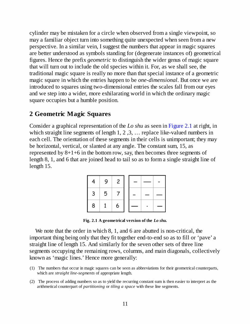
Consider a graphical representation of the Lo shu as seen in Figure 2.1 at right, inwhich straight line segments of length 1, 2 ,3, … replace like-valued numbers ineach cell. The orientation of these segments in their cells is unimportant; they maybe horizontal, vertical, or slanted at any angle. The constant sum, 15, asrepresented by 8+1+6 in the bottom row, say, then becomes three segments oflength 8, 1, and 6 that are joined head to tail so as to form a single straight line oflength 15.

Fig. 2.1 A geometrical version of the Lo shu.

We note that the order in which 8, 1, and 6 are abutted is non-critical, theimportant thing being only that they fit together end-to-end so as to fill or ‘pave’ astraight line of length 15. And similarly for the seven other sets of three linesegments occupying the remaining rows, columns, and main diagonals, collectivelyknown as ‘magic lines.’ Hence more generally:

(1) The numbers that occur in magic squares can be seen as abbreviations for their geometrical counterparts,which are straight line-segments of appropriate length.

(2) The process of adding numbers so as to yield the recurring constant sum is then easier to interpret as thearithmetical counterpart of partitioning or tiling a space with these line segments.

11

The advantage of this view now emerges in an entirely novel contingency itimmediately suggests. For just as line segments can pave longer segments, so areascan pave larger areas, volumes can pack roomier volumes, and so on up throughhigher dimensions. In traditional magic squares, we add numbers so as to form aconstant sum, which is to say, we ‘pave’ a one-dimensional space with one-dimensional ‘tiles.’ What happens beyond the one dimensional case?

Geometric or, less formally, geomagic is the term I use for a magic square inwhich higher dimensional geometrical shapes (or tiles or pieces) may appear in thecells instead of numbers. For the moment we shall dwell on flat, or two-dimensional shapes, although non-planar figures of 3 or higher dimensions mayequally be used. The orientation of each shape within its cell is unimportant. Suchan array of N × N geometrical pieces is called magic when the N entries occurringin each row, each column, as well as in both main diagonals, can be fitted togetherjigsaw-wise to produce an identical shape in each case. In tessellating thisconstant region or target, pieces are allowed to be flipped. As with numerical, orwhat I now call numagic squares, geomagic squares showing repeated entries aredenoted (and deemed) trivial or degenerate, which are terms we shall have needof more often. Rotated or reflected versions of the same geomagic square arecounted identical, as are rotations and reflections of the target. A square of size N ×N is said to be of order N. We say that a geomagic square is of dimension D whenits constituent pieces are all D-dimensional. This is an informal introduction togeomagic squares; for a formal definition see Appendix I. In the following, ourconcern will be almost exclusively with 2-D, or two-dimensional squares.

Figure 2.2 shows a 3×3 two-dimensional geomagic square in which the target isitself a square. Any 3 entries in a straight line can be assembled to pave this samesquare-shape without gaps or overlaps, as illustrated to right and below. Note howsome pieces appear one way in one target, while flipped and/or rotated in another.Thin grid lines on pieces within the square help identify their precise shape andrelative size.

12

Fig. 2.2 A 3 × 3 geomagic square.

At the top is a smaller 3 × 3 square with numbers indicating the areas ofcorresponding pieces in the geomagic square, expressed in units of half grid-squares. Since the three pieces in each row, column, and diagonal tile the sameshape, the sum of their areas must be the same. This is, therefore, an ordinarynumagic square (or one-dimensional geomagic square) with a constant sum equalto the target area. Analogous area squares for many geomagic squares are oftendegenerate because differently shaped pieces may share equal areas.

The concept of geometric magic squares grew out of an original impulse tocreate a pictorial representation of the algebraic square shown in Figure 2.3, aformula due to the 19th century French mathematician Édouard Lucas[5] thatdescribes the structure of every 3×3 numagic square. The Lo shu, for example, isthat instance of the formula in which a = 3, b = 1, and c = 5. From here on theterms formula and generalization will be used interchangeably.

The idea underlying this pictorial representation was as follows. Suppose thethree variables in the formula are each represented by a distinct planar shape. Thenthe entry c + a could be shown as shape c appended to shape a, while the entry c –a would become shape c from which shape a has been excised. And so on for theremaining entries. A back-of-the-envelope trial then lead to Figure 2.4, in which a

13

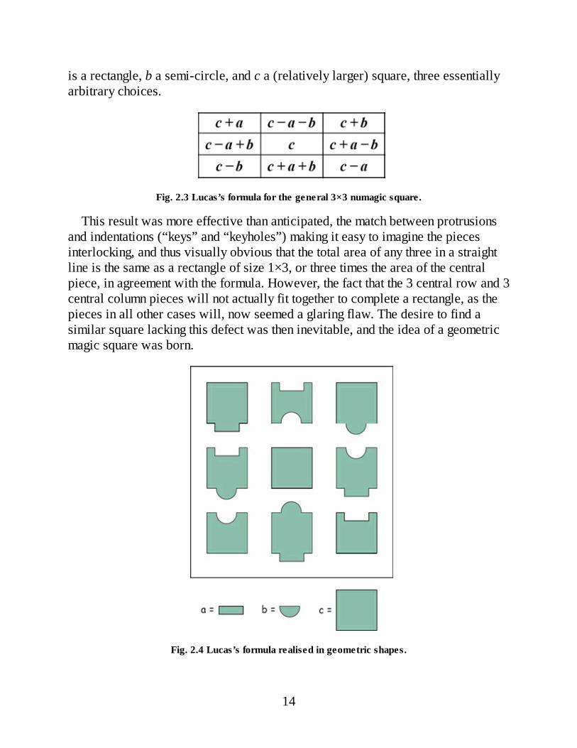
is a rectangle, b a semi-circle, and c a (relatively larger) square, three essentiallyarbitrary choices.

Fig. 2.3 Lucas’s formula for the general 3×3 numagic square.

This result was more effective than anticipated, the match between protrusionsand indentations (“keys” and “keyholes”) making it easy to imagine the piecesinterlocking, and thus visually obvious that the total area of any three in a straightline is the same as a rectangle of size 1×3, or three times the area of the centralpiece, in agreement with the formula. However, the fact that the 3 central row and 3central column pieces will not actually fit together to complete a rectangle, as thepieces in all other cases will, now seemed a glaring flaw. The desire to find asimilar square lacking this defect was then inevitable, and the idea of a geometricmagic square was born.

Fig. 2.4 Lucas’s formula realised in geometric shapes.

14

It was not until later, however, that the relationship between geometric andtraditional magic squares became clear. For, as we have seen, although the termgeometric magic square may seem to suggest a certain kind of magic square, infact things are the other way around. On the contrary, it is ordinary magic squaresthat turn out to be a special kind of geometric magic square, the kind that use one-dimensional pieces.

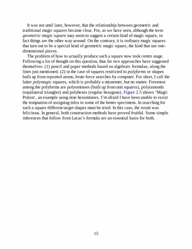
The problem of how to actually produce such a square now took centre stage.Following a lot of thought on this question, thus far two approaches have suggestedthemselves: (1) pencil and paper methods based on algebraic formulae, along thelines just mentioned. (2) in the case of squares restricted to polyforms or shapesbuilt up from repeated atoms, brute force searches by computer. For short, I call thelatter polymagic squares, which is probably a misnomer, but no matter. Foremostamong the polyforms are polyominoes (built up from unit squares), polyiamonds(equilateral triangles) and polyhexes (regular hexagons). Figure 2.5 shows ‘MagicPotion‘, an example using nine hexominoes. I’m afraid I have been unable to resistthe temptation of assigning titles to some of the better specimens. In searching forsuch a square different target shapes must be tried. In this case, the result wasfelicitous. In general, both construction methods have proved fruitful. Some simpleinferences that follow from Lucas’s formula are an essential basis for both.

15

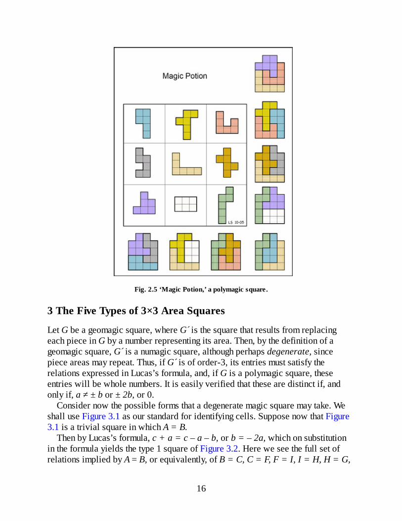
Fig. 2.5 ‘Magic Potion,’ a polymagic square.

3 The Five Types of 3×3 Area Squares

Let G be a geomagic square, where G is the square that results from replacingeach piece in G by a number representing its area. Then, by the definition of ageomagic square, G is a numagic square, although perhaps degenerate, sincepiece areas may repeat. Thus, if G is of order-3, its entries must satisfy therelations expressed in Lucas’s formula, and, if G is a polymagic square, theseentries will be whole numbers. It is easily verified that these are distinct if, andonly if, a ≠ ± b or ± 2b, or 0.

Consider now the possible forms that a degenerate magic square may take. Weshall use Figure 3.1 as our standard for identifying cells. Suppose now that Figure3.1 is a trivial square in which A = B.

Then by Lucas’s formula, c + a = c – a – b, or b = – 2a, which on substitutionin the formula yields the type 1 square of Figure 3.2. Here we see the full set ofrelations implied by A = B, or equivalently, of B = C, C = F, F = I, I = H, H = G,

16

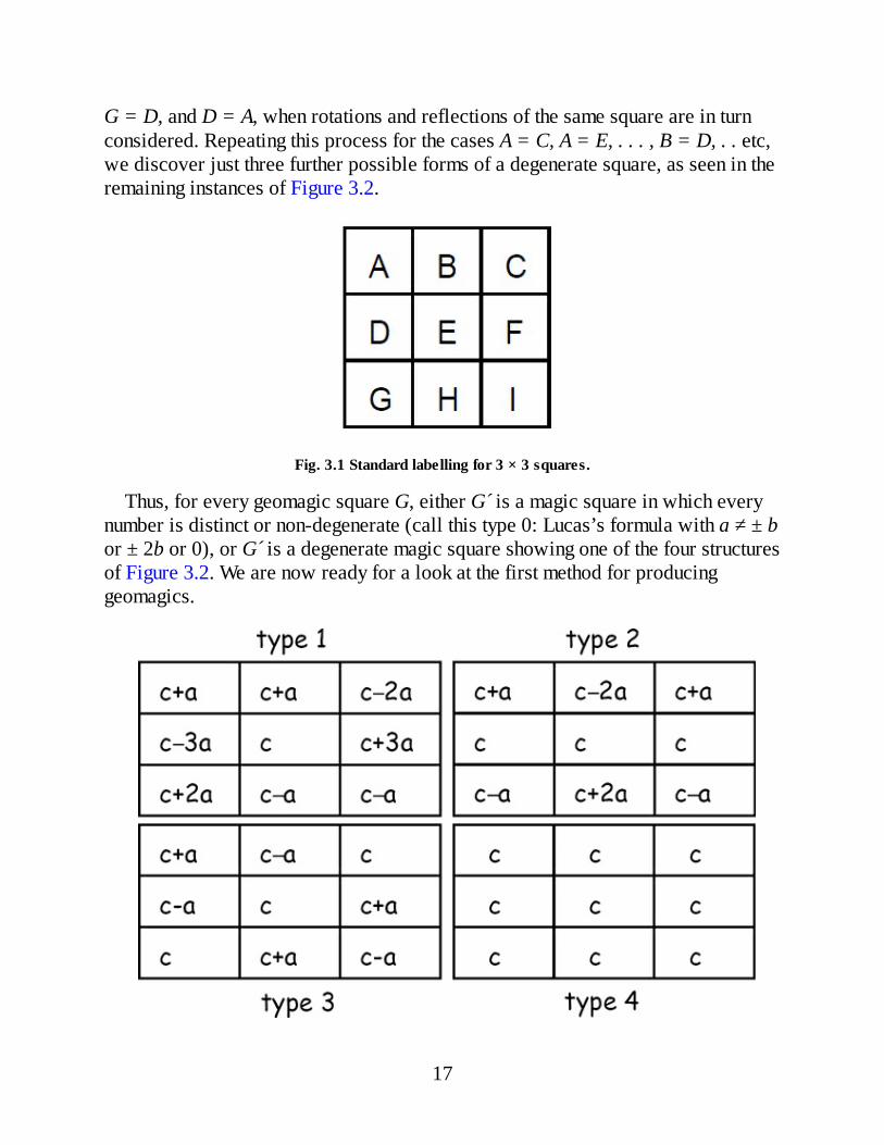
G = D, and D = A, when rotations and reflections of the same square are in turnconsidered. Repeating this process for the cases A = C, A = E, . . . , B = D, . . etc,we discover just three further possible forms of a degenerate square, as seen in theremaining instances of Figure 3.2.

Fig. 3.1 Standard labelling for 3 × 3 squares.

Thus, for every geomagic square G, either G is a magic square in which everynumber is distinct or non-degenerate (call this type 0: Lucas’s formula with a ≠ ± bor ± 2b or 0), or G is a degenerate magic square showing one of the four structuresof Figure 3.2. We are now ready for a look at the first method for producinggeomagics.

17

Fig. 3.2 The four degenerate types of magic square. Note that a type t square contains exactly 9 - 2Tdifferent entries.

4 Construction by Formula

As discussed previously, every numerical magic square has a primitivegeometrical analog using straight line-segments. We have only to broaden theselines into strips or rectangles of same height to result in a two-dimensionalgeomagic square, the target then being a longer strip that is formed simply byconcatenating the shorter ones occupying each magic line (i.e., each row, column,and diagonal). By suitable choice of rectangle height, the target can even be made asquare, as in the example based on the Lo shu shown in Figure 4.1.

18

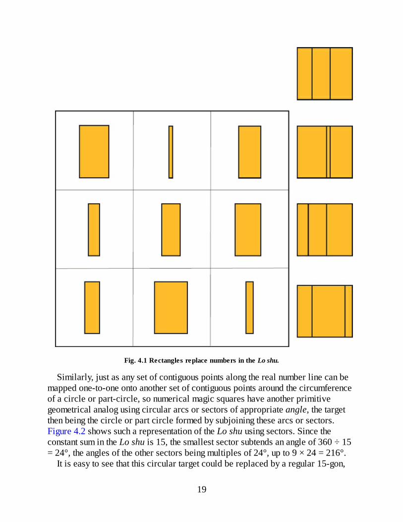
Fig. 4.1 Rectangles replace numbers in the Lo shu.

Similarly, just as any set of contiguous points along the real number line can bemapped one-to-one onto another set of contiguous points around the circumferenceof a circle or part-circle, so numerical magic squares have another primitivegeometrical analog using circular arcs or sectors of appropriate angle, the targetthen being the circle or part circle formed by subjoining these arcs or sectors.Figure 4.2 shows such a representation of the Lo shu using sectors. Since theconstant sum in the Lo shu is 15, the smallest sector subtends an angle of 360 ÷ 15= 24°, the angles of the other sectors being multiples of 24°, up to 9 × 24 = 216°.

It is easy to see that this circular target could be replaced by a regular 15-gon,

19

the sectors then changing to 15-gon segments of corresponding size. Likewise, thesectors in Figure 4.2 could be changed into annular segments, the target thenbecoming a ring with a central hole, or central 15-gon hole. Further variations mayoccur to the reader. By combining the straight line segment and circular arcinterpretations, numerical squares could equally be mapped onto 3-D helicalsegments.

The rectangles and sectors in Figures 4.1 and 4.2 can be further elaborated.Earlier I spoke simplistically of ‘broadening the line segments into strips of sameheight.’ A better way of conceiving this is to think of the broadened strip as justtwo 1-D segments of same length, one above the other, their ends joined by twostraight vertical lines so as to form a rectangle. However, it is not necessary thatthese lines be straight, only that they be congruent. Imagine a piece formed by apile of contiguous line segments, all parallel to each other, and yet shifted to left orright so that their ends describe some non-linear profile, as in Figure 4.3.

20

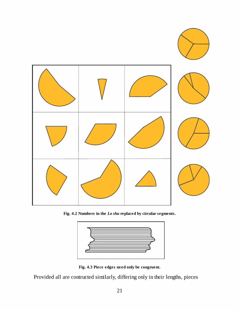
Fig. 4.2 Numbers in the Lo shu replaced by circular segments.

Fig. 4.3 Piece edges need only be congruent.

Provided all are contructed similarly, differing only in their lengths, pieces

21

constructed in this way can again be concatenated to form a long, thin target whoseends are sculpted with the same curve. Similar remarks apply to circular segments,a striking example of the kind of profile just mentioned being realized in Figure20.13 in the section on picture-preserving geomagic squares in Part 3.

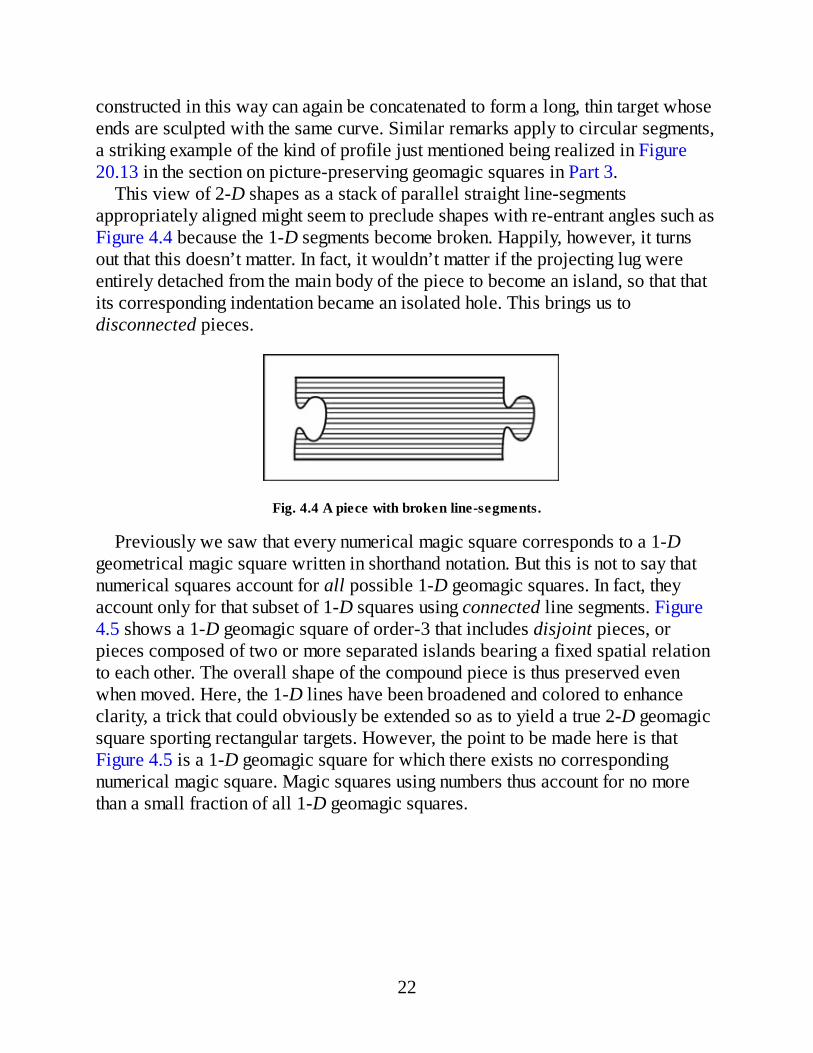
This view of 2-D shapes as a stack of parallel straight line-segmentsappropriately aligned might seem to preclude shapes with re-entrant angles such asFigure 4.4 because the 1-D segments become broken. Happily, however, it turnsout that this doesn’t matter. In fact, it wouldn’t matter if the projecting lug wereentirely detached from the main body of the piece to become an island, so that thatits corresponding indentation became an isolated hole. This brings us todisconnected pieces.

Fig. 4.4 A piece with broken line-segments.

Previously we saw that every numerical magic square corresponds to a 1-Dgeometrical magic square written in shorthand notation. But this is not to say thatnumerical squares account for all possible 1-D geomagic squares. In fact, theyaccount only for that subset of 1-D squares using connected line segments. Figure4.5 shows a 1-D geomagic square of order-3 that includes disjoint pieces, orpieces composed of two or more separated islands bearing a fixed spatial relationto each other. The overall shape of the compound piece is thus preserved evenwhen moved. Here, the 1-D lines have been broadened and colored to enhanceclarity, a trick that could obviously be extended so as to yield a true 2-D geomagicsquare sporting rectangular targets. However, the point to be made here is thatFigure 4.5 is a 1-D geomagic square for which there exists no correspondingnumerical magic square. Magic squares using numbers thus account for no morethan a small fraction of all 1-D geomagic squares.

22

Fig. 4.5 A square using disconnected pieces.

Just as with linear pieces, so circular arc pieces do not have to be connected.Figure 4.6 shows a 3×3 square using disjoint arcs, their unit segments heresimplified into single colored dots. Once again, such disconnected pieces cannotbe represented by single numbers.

Of course, the trouble with geomagic squares of the type seen in Figures 4.1 and4.2 is that they are really nothing more than the same old numerical magic square inalternate guise. The question is: how do we go about producing more interesting 2-D geomagics such as the first one looked at in Figure 2.2, which are somethingother than just a geometrical rehash of an arithmetical square? One approach is tostart with a trivial geomagic square based on a trivial algebraic formula, and thento de-trivialise this by adding appropriate keys and keyholes. I call algebraicsquares, trivial or otherwise, that are used in this way, templates. An example willclarify.

23

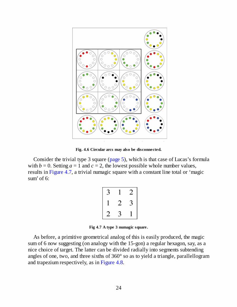
Fig. 4.6 Circular arcs may also be disconnected.

Consider the trivial type 3 square (page 5), which is that case of Lucas’s formulawith b = 0. Setting a = 1 and c = 2, the lowest possible whole number values,results in Figure 4.7, a trivial numagic square with a constant line total or ‘magicsum’ of 6:

Fig 4.7 A type 3 numagic square.

As before, a primitive geometrical analog of this is easily produced, the magicsum of 6 now suggesting (on analogy with the 15-gon) a regular hexagon, say, as anice choice of target. The latter can be divided radially into segments subtendingangles of one, two, and three sixths of 360° so as to yield a triangle, parallellogramand trapezium respectively, as in Figure 4.8.

24

Fig 4.8 A substrate or trivial geomagic square.

The hexagons show the two ways in which the 3 pieces in each line assemble tocomplete the target. I call such an initial, necessarily trivial geomagic square thathas yet to be elaborated, a substrate. Detrivializing this substrate so as to yield 9distinct piece-shapes is then merely a matter of assigning a nominal shape (a smalllug, say) to variable b in the type 3 formula, to result in the pattern of keys (+b) andkeyholes (–b) seen in Figure 4.9.

25

Fig 4.9 The trivial substrate detrivialised.

This is now a non-trivial 2-D geomagic square that is not simply a numericalmagic square in different guise. Note that the keys and keyholes may be of anyshape, provided only they remain within piece boundaries. They are thus in a sensegeometric variables, in that they are arbitrary shapes that can be taken as standingfor any other shape we might choose instead. The strong effect of an alternativechoice of key/keyhole shape can be seen from Magic Crystals in Figure 4.10,which is a polymagic square, identical to Figure 4.9, except that the key shape isnow a unit triangle belonging to the underlying isometric grid.

A striking result of this change is that the identity of the keys and keyholes assuch now becomes lost to sight, making it far more difficult for the viewer todiscern the principle of construction. So although Figure 4.10 is the prettierpicture, as well as a greater feat of illusion, it is better understood as a particularinstance of Figure 4.9, which provides the blueprint for an entire family ofgeomagic squares.

There are in fact two kinds of key/keyhole at work, in Figure 4.9; one obvious,the lug, the other invisible. It is again a triangle, the 60° hexagon segment thatcorresponds to variable a in Lucas’s formula, and is half that of the 120° segmentcorresponding to variable c, the parallelogram. The effect of appending this a-shaped “key” to c is thus indistinguishable from enlarging c (the segment angle

26

increases), and the effect of excizing the a-shaped key from c is indistinguishablefrom reducing c (the segment angle decreases). Similar effects are at work inFigure 4.1, where the rectangular “keys” and “keyholes” represented by both a andb merely increase or decrease the length of rectangle c. Call the latter “size-altering” keys/keyholes to distinguish them from “lug-type” keys/ keyholes. Figure4.11 shows another geometrical analog of Lucas’s formula in which the variables aand b are now both represented by lug-type keys and keyholes.

Fig 4.10 ‘Magic Crystals’ The principle of construction is difficult to detect.

Looking again at Lucas’s formula, we see that the trivial square started with hereis a uniform array with c in each cell, giving rise to a substrate composed of 9identical pieces. It took a little while to arrive at the choice of 9 squares. Mydifficulty was in seeing how two keys on one piece, whatever its shape, could bemade to marry with two keyholes on another piece of same shape (as for examplein the centre column), as well as two single keyholes on two separate pieces (e.g.in the bottom row). The T-shaped target provided a solution, the only one I havebeen able to find. Figure 4.12 shows a different rendering of Figure 4.11 usingpolyominoes. Variable c is now a square 16-omino, a a square tetromino and b adomino. The target remains a T-shape. See again how the identity of the keys andkeyholes disappears from view with the change to polyominoes.

27

Fig. 4.11 Lucas’s formula used as template.

Fig. 4.12 Polyominoes obscure the keys and keyholes.

28

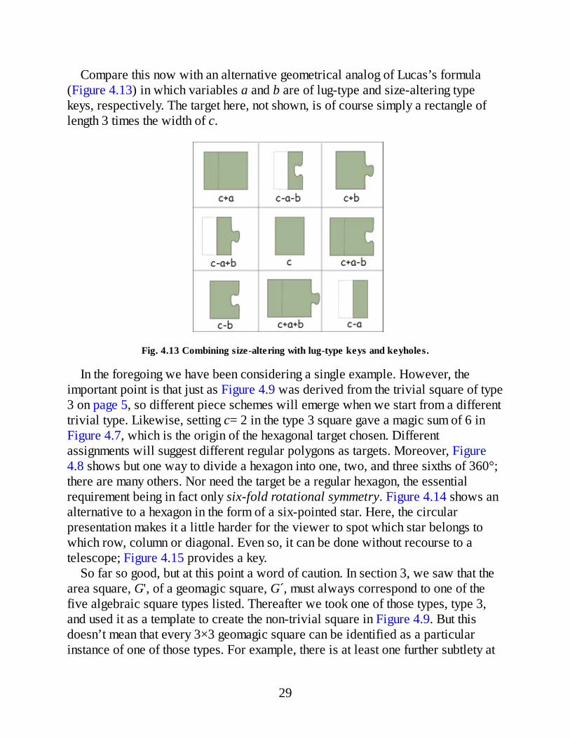
Compare this now with an alternative geometrical analog of Lucas’s formula(Figure 4.13) in which variables a and b are of lug-type and size-altering typekeys, respectively. The target here, not shown, is of course simply a rectangle oflength 3 times the width of c.

Fig. 4.13 Combining size-altering with lug-type keys and keyholes.

In the foregoing we have been considering a single example. However, theimportant point is that just as Figure 4.9 was derived from the trivial square of type3 on page 5, so different piece schemes will emerge when we start from a differenttrivial type. Likewise, setting c= 2 in the type 3 square gave a magic sum of 6 inFigure 4.7, which is the origin of the hexagonal target chosen. Differentassignments will suggest different regular polygons as targets. Moreover, Figure4.8 shows but one way to divide a hexagon into one, two, and three sixths of 360°;there are many others. Nor need the target be a regular hexagon, the essentialrequirement being in fact only six-fold rotational symmetry. Figure 4.14 shows analternative to a hexagon in the form of a six-pointed star. Here, the circularpresentation makes it a little harder for the viewer to spot which star belongs towhich row, column or diagonal. Even so, it can be done without recourse to atelescope; Figure 4.15 provides a key.

So far so good, but at this point a word of caution. In section 3, we saw that thearea square, G', of a geomagic square, G´, must always correspond to one of thefive algebraic square types listed. Thereafter we took one of those types, type 3,and used it as a template to create the non-trivial square in Figure 4.9. But thisdoesn’t mean that every 3×3 geomagic square can be identified as a particularinstance of one of those types. For example, there is at least one further subtlety at

29

work here about which we need to be aware.

Fig. 4.14 ‘Star Formation’ Evil rats on no star live.

30

Fig. 4.15 Key to ‘Star Formation’.

Consider the 3×3 square in Figure 4.16. The keys and keyholes belonging toeach of the three pieces occupying the main diagonal (\) re-echo the congruentpiece profiles of Figure 4.3, except in this case applied to circular segments ratherthan rectangular pieces. That is, the projecting profile on one radial edge is theimage of the indented profile on the other radial edge. It is informative toreconstruct the algebraic template of which this square is a geometricalinterpretation. To this end, substituting distinct variables A, B, and C for the threedifferent segment sizes (60°, 180°, 120°, respectively), with a and b for the twodistinct keys, brings to light the algebraic square of Figure 4.17. It is a square thatwill not be magic unless the sum of the entries occupying the co-diagonal (/) ismade equal to the sum of the three entries in every other line. That is, when 3C = A

+ B + C, or .

31

Fig. 4.16 A square using circular segments of three sizes.

Fig. 4.17 A template for Figure 4.16.

The result is then a trivial square formed by A, B, and (A+B)/2 accompanied by adetrivializing pattern of a’s and b’s that includes a curious feature. The three entrieson the main diagonal all contain ‘a – a ’, a term we would normally ignore or omitbecause redundant, but is here an intrinsic and necessary part of the template. Sucha square reminds us that in applying the template technique we wander somewhatfrom the path of everyday mathematics and enter a weird world in which the verymode of expression used to identify relations becomes as important as thoserelations themselves. For example, as the reader may like to verify, Figure 4.17 canbe shown to be simply an alternative expression of Lucas’s formula, which is tosay, a square of type 0. But whereas it supplies a template for the 2-D square inFigure 4.16, Lucas’s formula emphatically does not, even though the two algebraicsquares are mathematically isomorphic.

Little wonder then that the devising of algebraic templates is something of an art,

32

involving at times an uncomfortable reliance on intuition tempered only by trial anderror. This is a curious development in what was supposedly to be an exercise inalgebra. In defence, I can only say that the challenge confronted in creatinggeomagic squares has proved too demanding in every other direction, save that ofbrute force searches using a computer. But better, I thought, a slipshod method thatproduces results of some kind, rather than a more respectable approach that yieldsnone. And whatever its shortcomings, the template method has certainly proveditself fruitful, as I hope the many examples to be found in these pages will attest.

The brute force searches by computer just referred to are applicable only in thecase of squares using polyforms. Special instances of the latter are polyominoes,polyiamonds and polyhexes, which produce tilings showing a greater regularitythan that found in other cases. It is this regularity that enables computer programs tobe written that are able to identify all the tilings of a given target using a given setof pieces. However, less regular polyforms exist, as exampled in Figure 4.18,which is again based on the template of Figure 4.17.

Here the target is a ‘medallion’ due to Michael Hirschhorn, who discovered it inconnection with some teaching work involving pentagonal tiles conducted at theUniversity of New South Wales in Australia in 1976[6] [7]. The medallion isreally the central hub of an infinite tessellation showing six-fold rotationalsymmetry; it can be extended outwards indefinitely so as to cover the entire plane.The basic tile used is an equilateral pentagon that is among ten pentagonal tilesindependently identified at around the same time by Marjorie Rice, a San Diegohousewife with a mathematically inventive bent [8] [9], Complicated as it mayseem at first sight, examination will show how the radial profiles of each piece areexactly mirrored by those in the square of Figure 4.16. Figure 20.13 is yet anotherexample modelled on the same template.

There is, in fact, a good deal more to be said about the construction ofgeomagics based on the template technique. However, the peculiarities of order-3squares make them an unsuitable vehicle for explaining certain points. In thesection on 4×4 geomagics we return to this topic, but for now we pass on.

33

Fig. 4.18 A square using Michael Hirschhorn’s medallion as target.

5 Construction by Computer

The five area types discussed before are critical in designing a program able toseek for 3×3 polymagic squares, since besides the need to specify the target shaperequired, we must also specify the sizes of the pieces to be used. An example willclarify how one such program works.

Suppose we seek a 3×3 polymagic square P using nine polyominoes of equalsize; i.e. the area square is of type 4 above. From Lucas’s formula we know that thearea of its target is an integer divisible by 3, making a 3×5 rectangle, say, asuitable choice of shape. All pieces will then be of size 15÷3 = 5, or pentominoes,of which there exist exactly 12 distinct exemplars. Number these from 1 to 12. Abrute force search for a set of 9 pentominoes able to construct P is then simpleenough, given first a list L of all the possible sets of 3 distinct pentominoes thatwill tile a 3×5 rectangle. Every entry in L is thus a triad of distinct numbers in therange 1 to 12. Taking now every possible combination of three distinct entries oneat a time, say {R,S,T}, {U,V,W} and {X,Y,Z}, we imagine these entered into a 3×3array to produce a square whose rows are now magic because they containpentomino triads taken from L that therefore tile the target; see Figure 5.1.

34

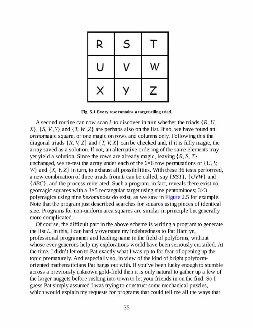
Fig. 5.1 Every row contains a target-tiling triad.

A second routine can now scan L to discover in turn whether the triads {R, U,X}, {S, V ,Y} and {T, W ,Z} are perhaps also on the list. If so, we have found anorthomagic square, or one magic on rows and columns only. Following this thediagonal triads {R, V, Z} and {T, V, X} can be checked and, if it is fully magic, thearray saved as a solution. If not, an alternative ordering of the same elements mayyet yield a solution. Since the rows are already magic, leaving {R, S, T}unchanged, we re-test the array under each of the 6×6 row permutations of {U, V,W} and {X, Y, Z} in turn, to exhaust all possibilities. With these 36 tests performed,a new combination of three triads from L can be called, say {RST}, {UVW} and{ABC}, and the process reiterated. Such a program, in fact, reveals there exist nogeomagic squares with a 3×5 rectangular target using nine pentominoes; 3×3polymagics using nine hexominoes do exist, as we saw in Figure 2.5 for example.Note that the program just described searches for squares using pieces of identicalsize. Programs for non-uniform area squares are similar in principle but generallymore complicated.

Of course, the difficult part in the above scheme is writing a program to generatethe list L. In this, I can hardly overstate my indebtedness to Pat Hamlyn,professional programmer and leading name in the field of polyforms, withoutwhose ever generous help my explorations would have been seriously curtailed. Atthe time, I didn’t let on to Pat exactly what I was up to for fear of opening up thetopic prematurely. And especially so, in view of the kind of bright polyform-oriented mathematicians Pat hangs out with. If you’ve been lucky enough to stumbleacross a previously unknown gold-field then it is only natural to gather up a few ofthe larger nuggets before rushing into town to let your friends in on the find. So Iguess Pat simply assumed I was trying to construct some mechanical puzzles,which would explain my requests for programs that could tell me all the ways that

35

a certain shape could be tiled by certain other shapes. But whatever he thought, henot only provided me with an entire suite of his sophisticated programs, in emailafter email, time and trouble were not spared in responding at length to my endlessquestions, and even in adopting his software to my specific demands. Thus, if thereis any credit due for tracking down the polymagic squares to be seen in these pagesthen a very big chunk of it belongs to Pat Hamlyn, the real brains behind theresearch, and a warm and generous man besides.

So much for a brief sketch of the two present known methods for producing 2-Dmagic squares. We shall now take a look at some example squares of order 3.

6 3×3 Squares

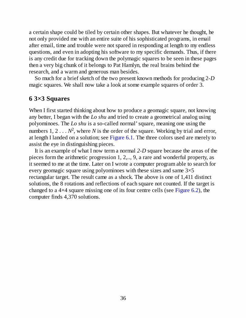
When I first started thinking about how to produce a geomagic square, not knowingany better, I began with the Lo shu and tried to create a geometrical analog usingpolyominoes. The Lo shu is a so-called normal’ square, meaning one using thenumbers 1, 2 . . . N2, where N is the order of the square. Working by trial and error,at length I landed on a solution; see Figure 6.1. The three colors used are merely toassist the eye in distinguishing pieces.

It is an example of what I now term a normal 2-D square because the areas of thepieces form the arithmetic progression 1, 2,.., 9, a rare and wonderful property, asit seemed to me at the time. Later on I wrote a computer program able to search forevery geomagic square using polyominoes with these sizes and same 3×5rectangular target. The result came as a shock. The above is one of 1,411 distinctsolutions, the 8 rotations and reflections of each square not counted. If the target ischanged to a 4×4 square missing one of its four centre cells (see Figure 6.2), thecomputer finds 4,370 solutions.

36

Fig. 6.1 One of 1,411 normal squares with 3×5 rectangular target.

If the target is a 4×4 square minus one of its inner edge cells (see Figure 6.3)there are 16,465 solutions.

Fig. 6.2 One among 4,370 normal squares using a 4×4 target with inner hole.

37

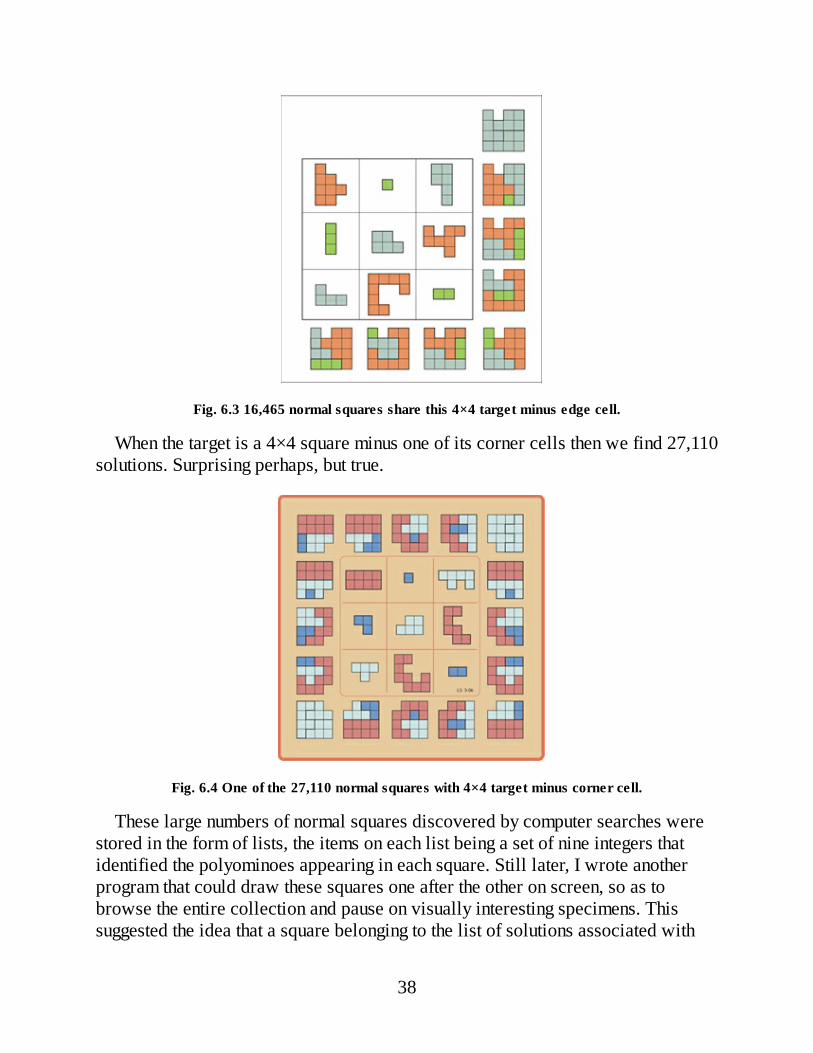
Fig. 6.3 16,465 normal squares share this 4×4 target minus edge cell.

When the target is a 4×4 square minus one of its corner cells then we find 27,110solutions. Surprising perhaps, but true.

Fig. 6.4 One of the 27,110 normal squares with 4×4 target minus corner cell.

These large numbers of normal squares discovered by computer searches werestored in the form of lists, the items on each list being a set of nine integers thatidentified the polyominoes appearing in each square. Still later, I wrote anotherprogram that could draw these squares one after the other on screen, so as tobrowse the entire collection and pause on visually interesting specimens. Thissuggested the idea that a square belonging to the list of solutions associated with

38

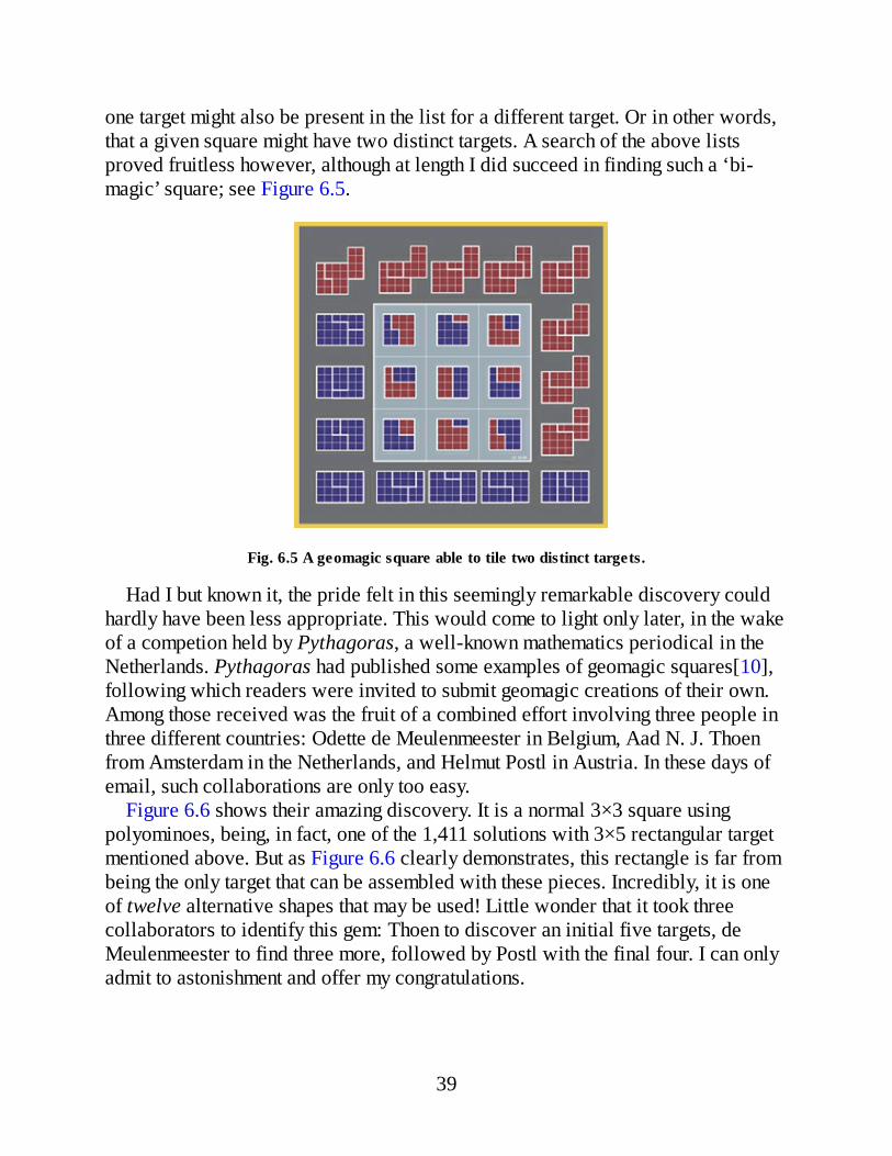
one target might also be present in the list for a different target. Or in other words,that a given square might have two distinct targets. A search of the above listsproved fruitless however, although at length I did succeed in finding such a ‘bi-magic’ square; see Figure 6.5.

Fig. 6.5 A geomagic square able to tile two distinct targets.

Had I but known it, the pride felt in this seemingly remarkable discovery couldhardly have been less appropriate. This would come to light only later, in the wakeof a competion held by Pythagoras, a well-known mathematics periodical in theNetherlands. Pythagoras had published some examples of geomagic squares[10],following which readers were invited to submit geomagic creations of their own.Among those received was the fruit of a combined effort involving three people inthree different countries: Odette de Meulenmeester in Belgium, Aad N. J. Thoenfrom Amsterdam in the Netherlands, and Helmut Postl in Austria. In these days ofemail, such collaborations are only too easy.

Figure 6.6 shows their amazing discovery. It is a normal 3×3 square usingpolyominoes, being, in fact, one of the 1,411 solutions with 3×5 rectangular targetmentioned above. But as Figure 6.6 clearly demonstrates, this rectangle is far frombeing the only target that can be assembled with these pieces. Incredibly, it is oneof twelve alternative shapes that may be used! Little wonder that it took threecollaborators to identify this gem: Thoen to discover an initial five targets, deMeulenmeester to find three more, followed by Postl with the final four. I can onlyadmit to astonishment and offer my congratulations.

39

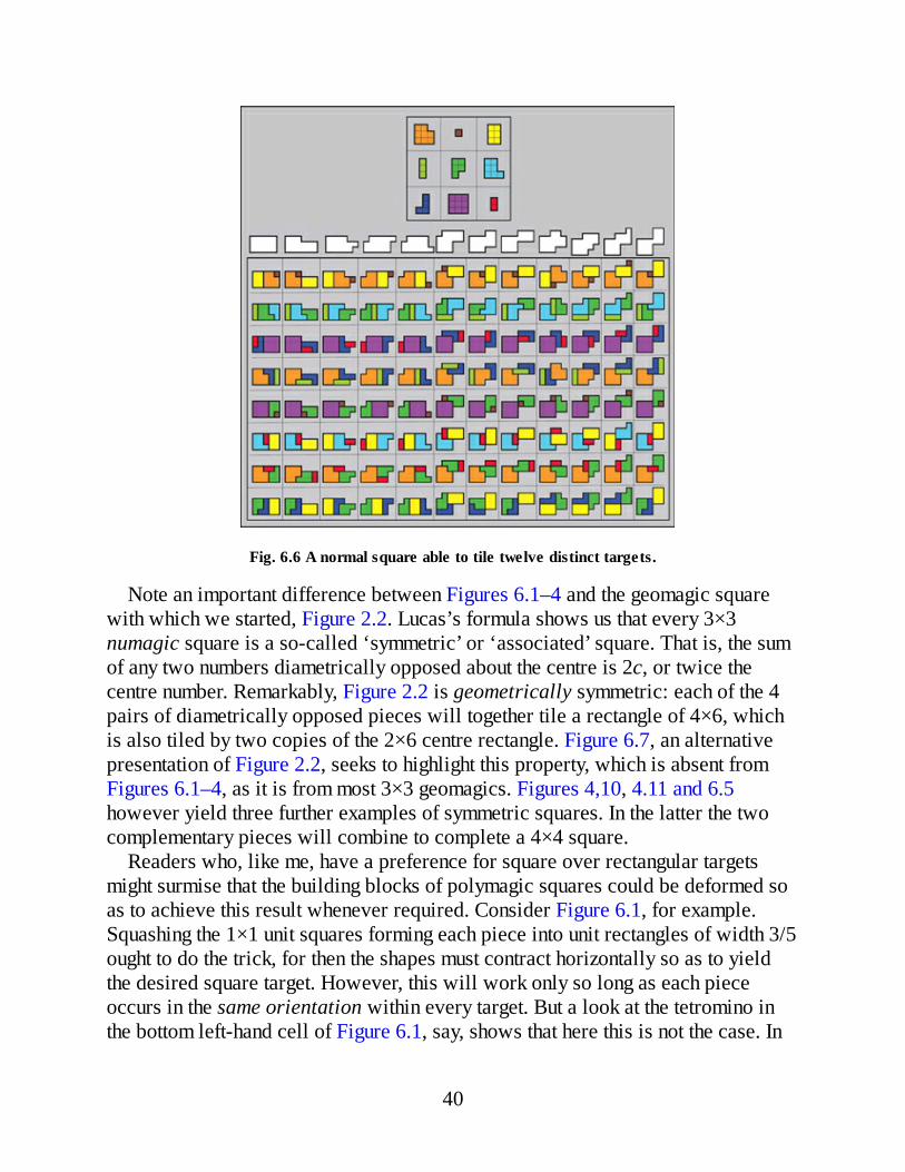
Fig. 6.6 A normal square able to tile twelve distinct targets.

Note an important difference between Figures 6.1–4 and the geomagic squarewith which we started, Figure 2.2. Lucas’s formula shows us that every 3×3numagic square is a so-called ‘symmetric’ or ‘associated’ square. That is, the sumof any two numbers diametrically opposed about the centre is 2c, or twice thecentre number. Remarkably, Figure 2.2 is geometrically symmetric: each of the 4pairs of diametrically opposed pieces will together tile a rectangle of 4×6, whichis also tiled by two copies of the 2×6 centre rectangle. Figure 6.7, an alternativepresentation of Figure 2.2, seeks to highlight this property, which is absent fromFigures 6.1–4, as it is from most 3×3 geomagics. Figures 4,10, 4.11 and 6.5however yield three further examples of symmetric squares. In the latter the twocomplementary pieces will combine to complete a 4×4 square.

Readers who, like me, have a preference for square over rectangular targetsmight surmise that the building blocks of polymagic squares could be deformed soas to achieve this result whenever required. Consider Figure 6.1, for example.Squashing the 1×1 unit squares forming each piece into unit rectangles of width 3/5ought to do the trick, for then the shapes must contract horizontally so as to yieldthe desired square target. However, this will work only so long as each pieceoccurs in the same orientation within every target. But a look at the tetromino inthe bottom left-hand cell of Figure 6.1, say, shows that here this is not the case. In

40

the bottom row and left-hand column targets it appears unchanged in orientation,but in the co-diagonal (/) target it is rotated. Following horizontal squashing, itwould therefore be too short to completely tile the latter target.

Fig. 6.7 Complementary piece pairs tile the same rectangle.

In fact, experience teaches that the interlocking relations within geomagics canbe very deceptive. Again and again, one feels convinced that some in significantdetail can be altered, only to find out that the change has disastrous consequenceselsewhere in the square. Figure 6.8(a) is one among a few examples found of ageomagic square in which the pieces appear neither rotated nor reflected in anytarget. This is perhaps unsurprising; just as a conventional magic square maycontain the number zero, so Figure 6.8(a) makes use of the ‘empty’ piece, with theresult that only eight pieces are involved. The constant orientation of these eightpieces means that the entire square can be stretched or squashed without affectingits geomagic properties, as shown in Figures 6.8(b) and (c). The target can then bea square (b), or even a parallelogram (d).

41

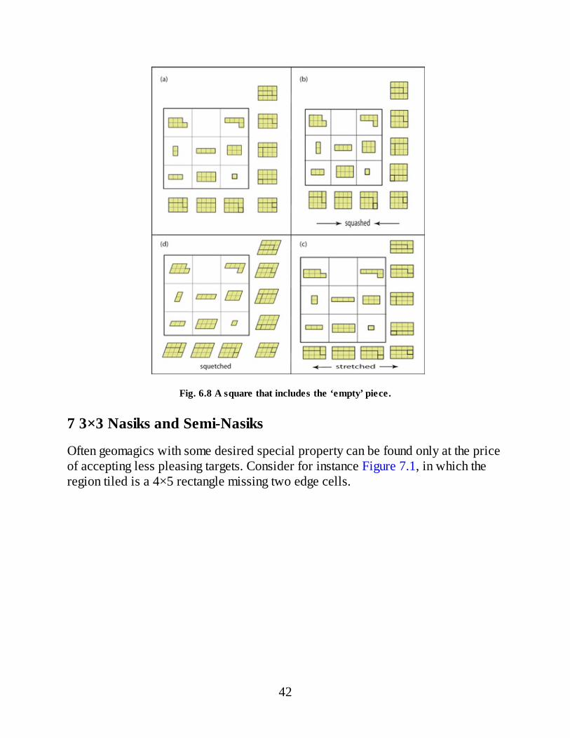
Fig. 6.8 A square that includes the ‘empty’ piece.

7 3×3 Nasiks and Semi-Nasiks

Often geomagics with some desired special property can be found only at the priceof accepting less pleasing targets. Consider for instance Figure 7.1, in which theregion tiled is a 4×5 rectangle missing two edge cells.

42

Fig. 7.1 A semi-nasik square.

The pieces used are of three sizes: 3 pentominoes, 3 hexominoes, and 3heptominoes, the areas forming a Latin square, seen above left. The subject ofLatin squares has a long history, abounding as it does with unsolved problems,some of them as many as 200 years old [11]. By a Latin square of order N, we referto a square of N2 entries composed of N distinct elements, each of which occursexactly once in every row and column. Here the entries happen to be numbers, butcould equally be elements of a different kind, such as letters or geometrical shapes.We shall have more to do with Latin squares when we come to 4×4 geomagics.

Figure 7.1 is an example of a square that is ‘semi-panmagic’ or ‘semi-nasik’.Fully panmagic or nasik2 squares (so named after the town in India where an early4×4 specimen was found) are those in which every diagonal, including the so-called ‘broken’ diagonals, AFH, BDI, CDH, and BFG, are also magic lines, whichis to say, their pieces tile the target. Note that AFH and BDI are parallel and hencenon-intersecting, as are CDH and BFG. Semi-nasik squares of 3×3 are thoseshowing a total of 4 magic diagonals that include the two main diagonals plus oneof these two parallel pairs. In Figure 7.1 the latter are AFH and BDI, as shown bythe targets at top.

There exist similar 3×3 geomagics with a total of 4 magic diagonals that aredifferent to those in semi-nasiks. These are squares in which the two maindiagonals, plus two broken diagonals that are non-parallel and thus intersecting are

43

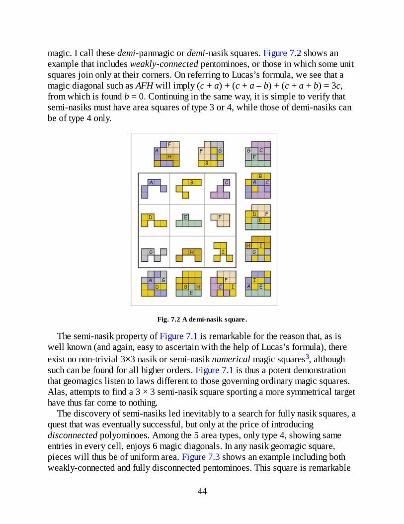
magic. I call these demi-panmagic or demi-nasik squares. Figure 7.2 shows anexample that includes weakly-connected pentominoes, or those in which some unitsquares join only at their corners. On referring to Lucas’s formula, we see that amagic diagonal such as AFH will imply (c + a) + (c + a – b) + (c + a + b) = 3c,from which is found b = 0. Continuing in the same way, it is simple to verify thatsemi-nasiks must have area squares of type 3 or 4, while those of demi-nasiks canbe of type 4 only.

Fig. 7.2 A demi-nasik square.

The semi-nasik property of Figure 7.1 is remarkable for the reason that, as iswell known (and again, easy to ascertain with the help of Lucas’s formula), thereexist no non-trivial 3×3 nasik or semi-nasik numerical magic squares3, althoughsuch can be found for all higher orders. Figure 7.1 is thus a potent demonstrationthat geomagics listen to laws different to those governing ordinary magic squares.Alas, attempts to find a 3 × 3 semi-nasik square sporting a more symmetrical targethave thus far come to nothing.

The discovery of semi-nasiks led inevitably to a search for fully nasik squares, aquest that was eventually successful, but only at the price of introducingdisconnected polyominoes. Among the 5 area types, only type 4, showing sameentries in every cell, enjoys 6 magic diagonals. In any nasik geomagic square,pieces will thus be of uniform area. Figure 7.3 shows an example including bothweakly-connected and fully disconnected pentominoes. This square is remarkable

44

for a further reason. Choose any three pieces belonging to any three of the fourcorner cells. There are 4 possible choices. The selected triad will tile the target inevery case. The resulting 16 near-square targets that encircle the 3×3 array makefor a pleasing mathematical ornament. A key to the square is shown in Figure 7.4.

It is a well-known property of nasik squares of any size that they remain nasikunder cyclic permutation of their rows and columns. This is nicely demonstratedwhen the plane is tiled with repeated copies of an N × N nasik square, with theresult that any arbitrarily selected N × N area will again be found to be a nasiksquare. This is illustrated in Figure 7.5 using the above 3×3 specimen.

The identification of 3×3 nasik and semi-nasik geomagics —there are many tobe found beside those shown here, as well as squares showing 0, 1, 3, or 5 magicdiagonals— raises an interesting question. As seen with the nasik-preservingcyclic permutations of rows and columns, unlike standard 3×3 geomagics, theentries in nasik and semi-nasik squares can be rearranged to yield still moregeomagic squares. But exactly how many distinct specimens can be thus formed?The non-existence of numagic nasiks or semi-nasiks means that this question hasnever before been addressed. A simple computer program provided the answer byexamining in turn every permutation of the 9 letters in Figure 7.4 (or Figure 3.1),which is interpreted as representing a nasik square exhibiting the 12 magic triads:ABC, DEF, GHI, ADG, BEH, CFI, AEI, BFG, CDH, CEG, AFH and BDI.

45

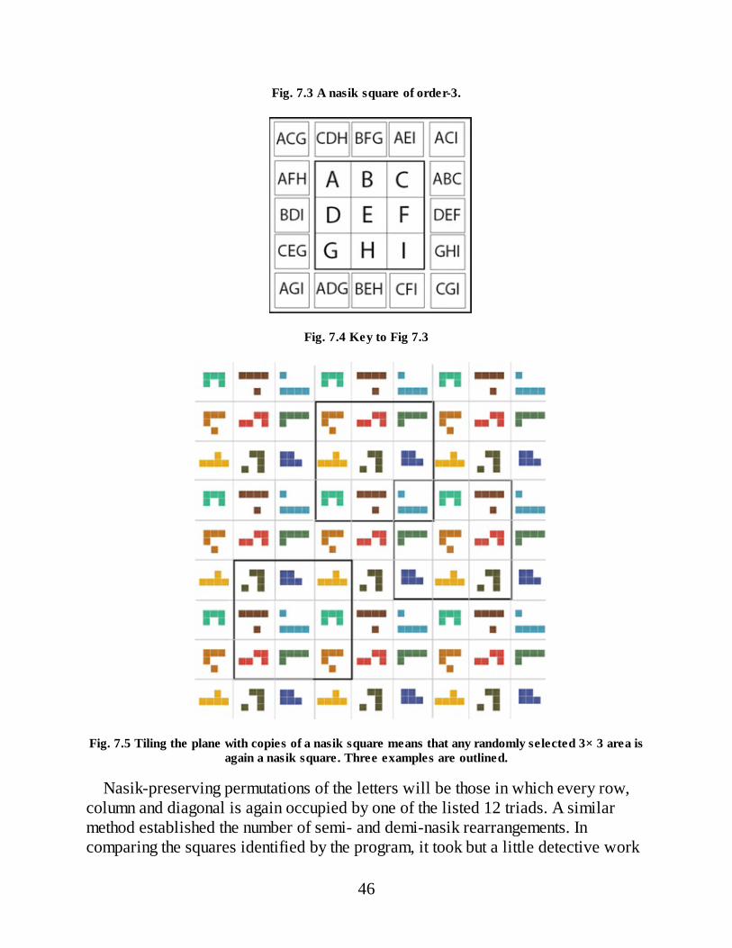
Fig. 7.3 A nasik square of order-3.

Fig. 7.4 Key to Fig 7.3

Fig. 7.5 Tiling the plane with copies of a nasik square means that any randomly selected 3× 3 area isagain a nasik square. Three examples are outlined.

Nasik-preserving permutations of the letters will be those in which every row,column and diagonal is again occupied by one of the listed 12 triads. A similarmethod established the number of semi- and demi-nasik rearrangements. Incomparing the squares identified by the program, it took but a little detective work

46

to unravel their relations so as to describe these in terms of a few basictransformations. As a matter of fact, these investigations were performed beforeever a nasik or semi-nasik geomagic square had actually been discovered. I wasthus in the curious position of having a pretty thorough understanding of 3×3 nasikand semi-nasik geomagic squares long before even knowing whether or not anyexisted.

The number of magic rearrangements for semi-nasiks is nine, rotations andreflections not counted. Two transformations (T1, T2), both of order-3, generate allnine, as diagrammed in Figure 7.6(a.) AFH and BDI are the two magic brokendiagonals. Demi-nasiks yield just four squares, as generated by transformation T3in Figure 7.6(b.) Nasik squares are still more prolix, T1 and T2 combining with thetwo transformations T4 and T5 shown in Figure 7.6(c,) as well as two furthertransformations that produce the 8 rotations and reflections of each square, to forma group of order-432. Thanks are due to my friend Michael Schweitzer foridentifying this as the affine general linear group AGL(2,3). In consequence, theentries in any 3×3 nasik geomagic square can always be permuted to produce atleast 432 ÷ 8 = 54 distinct squares, rotations and reflections not counted. Squaresthat result from permuting pieces in nasik or semi-nasik squares are themselvesalways nasik or semi-nasik, respectively.

Surprising as it may seem, there are still more magic triads to be found in Figure7.3 than the 16 appearing in the targets drawn. In all there are 36. They are asfollows:

47

Fig. 7.6 (a) Rearranging the pieces in a semimagic square gives rise to 9 variants. (b) Demi-magicrearrangements number 4. (c) TransformsT1,T2,T4, andT5 yield 54 variants of a nasik square.

We have seen that the pieces in Figure 7.3 can be rearranged so as to yield atleast 54 different nasik squares. Might it be that this large number of extra magictriads will allow even more to be formed? If so, the total must be a multiple of 54,since for every extra square, there will be its accompanying 53 nasik permutations.In fact a computer trial shows that this is not the case with Figure 7.3. But squareshaving this property can be found. The pieces in Figure 7.7, for example, another

48

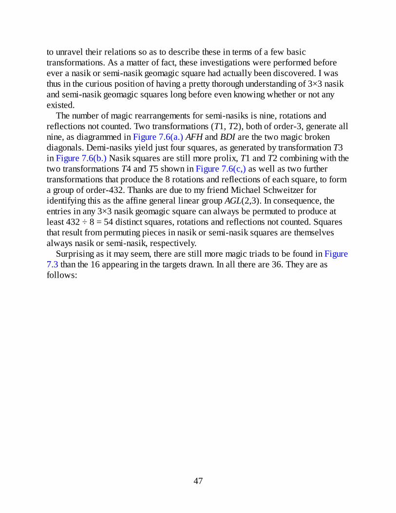
nasik square with a smaller number of magic triads, can be rearranged so as toyield 2 × 54 = 108 nasik squares. Its 31 magic triads are as follows:

Fig. 7.7 A nasik square using 9 pentominoes, normal, weakly-connected, and disjoint.

The reason for this doubling in numbers is not difficult to find. As the reader canverify, pieces E and I in Figure 7.7 can be switched, yet the square remainsgeomagic. Scrutiny shows that this will be possible only when the 6 triads, DFI,BHI, CGI, CEF, EGH, and BDE, are among the 31. This is a consequence of thefact that, following such a switch, all six of these triads will find themselvesoccupying rows, columns and diagonals. Hence a nasik square might have as fewas just six extra magic triads and still yield 108 different squares.

8 Special Examples of 3×3 Squares

Above we noted the existence of thousands of geomagics using pieces with areas

49

of 1, 2, . . . , 9 units. Since the areas are all different, their area squares are of type0. Research indicates that the fertility4 of a set of pieces falls dramatically as thenumber of same-sized pieces in the set increases. For example, the pieces in atype-2 square (page 15), exhibit just five different areas. Figure 8.1 shows anexample; the pieces are of sizes 4, 6, 8, 10 and 12. It is one of only three solutionsfound. 3×3 squares in which all the pieces are of same size are even rarer. Figures2.5 and 8.5 show examples using nine hexominoes and decominoes, respectively.

Fig. 8.1 Repeated piece sizes imply fewer solutions.

The target with central hole in Figure 8.1 is less a decorative flourish than aconsolation prize. To see why, suppose we seek a 3×3 polymagic square showing asolid square target. The target area must then be a square number that is a multipleof 3, or 3 times the area of the centre piece. The possibilities are thus 9, 36, 81, . . .. However, 9 is impossible because the pieces required would be too small toallow enough distinct shapes. 81 implies an average piece size of 81 ÷ 3 = 27,which is too large for a personal computer to handle because the numbers of piececombinations becomes prohibitively large. 36 seems hopeful. Let us begin with asearch for a square using nine dodecominoes, or polyominoes formed of 12 unitsquares. The program requires a list L of all the triads of dodecominoes that tile a6×6 square. There are 32,222 such triads. Being a longish list, it takes the programa while to check whether the triad of pieces in a candidate column/ diagonal is, oris not, in L. And with 36 permutations of each candidate square to test, there are a

50

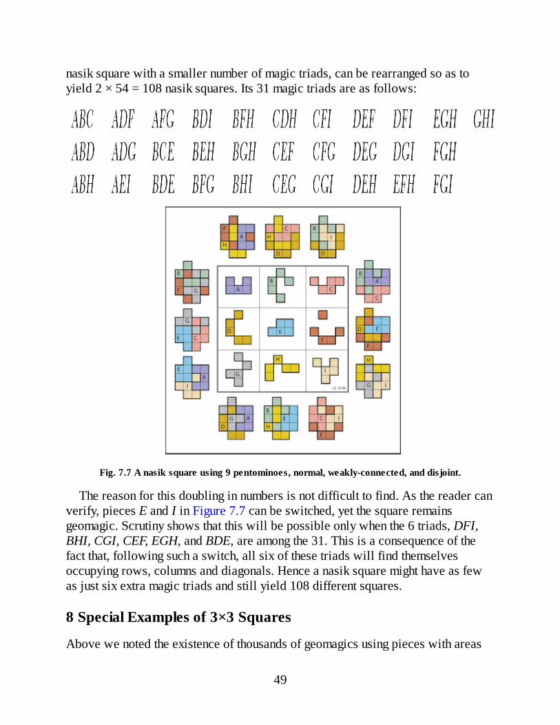
lot of checks to perform. Such a program ran for weeks on my PC, without findinga solution. Figure 8.2 shows one of several simple or orthomagic squaresdiscovered along the way. The latter are squares that are magic on rows andcolumns only.

Fig. 8.2 An orthomagic square using same-sized pieces.

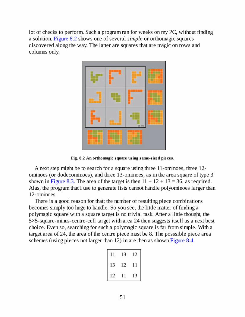
A next step might be to search for a square using three 11-ominoes, three 12-ominoes (or dodecominoes), and three 13-ominoes, as in the area square of type 3shown in Figure 8.3. The area of the target is then 11 + 12 + 13 = 36, as required.Alas, the program that I use to generate lists cannot handle polyominoes larger than12-ominoes.

There is a good reason for that; the number of resulting piece combinationsbecomes simply too huge to handle. So you see, the little matter of finding apolymagic square with a square target is no trivial task. After a little thought, the5×5-square-minus-centre-cell target with area 24 then suggests itself as a next bestchoice. Even so, searching for such a polymagic square is far from simple. With atarget area of 24, the area of the centre piece must be 8. The posssible piece areaschemes (using pieces not larger than 12) in are then as shown Figure 8.4.

51

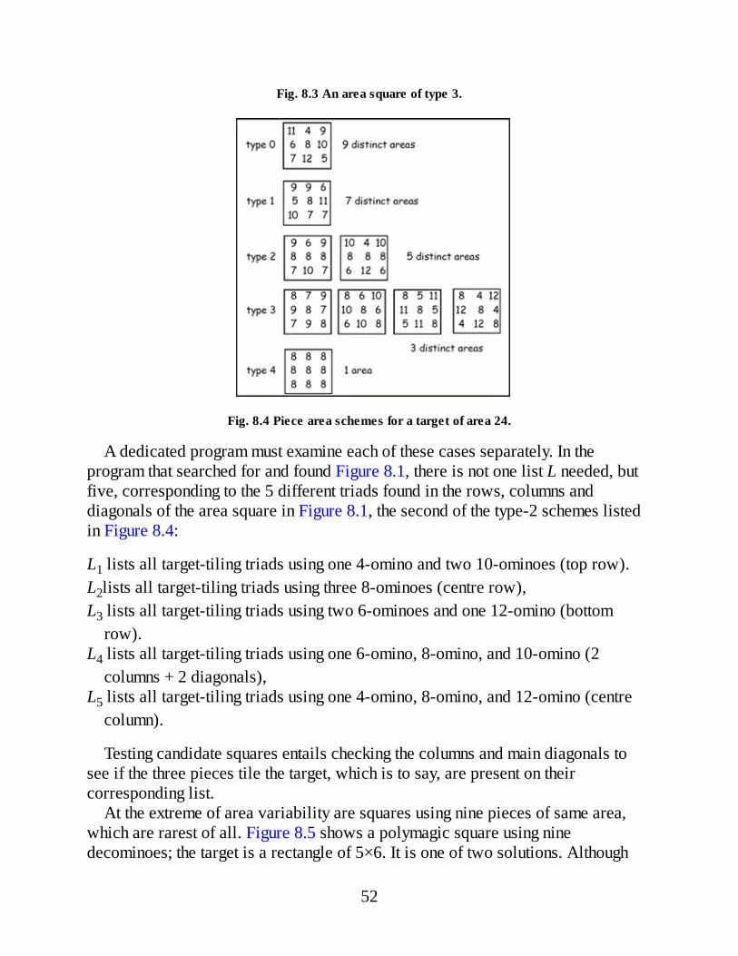
Fig. 8.3 An area square of type 3.

Fig. 8.4 Piece area schemes for a target of area 24.

A dedicated program must examine each of these cases separately. In theprogram that searched for and found Figure 8.1, there is not one list L needed, butfive, corresponding to the 5 different triads found in the rows, columns anddiagonals of the area square in Figure 8.1, the second of the type-2 schemes listedin Figure 8.4:

L1 lists all target-tiling triads using one 4-omino and two 10-ominoes (top row).L2lists all target-tiling triads using three 8-ominoes (centre row),L3 lists all target-tiling triads using two 6-ominoes and one 12-omino (bottom

row).L4 lists all target-tiling triads using one 6-omino, 8-omino, and 10-omino (2

columns + 2 diagonals),L5 lists all target-tiling triads using one 4-omino, 8-omino, and 12-omino (centre

column).

Testing candidate squares entails checking the columns and main diagonals tosee if the three pieces tile the target, which is to say, are present on theircorresponding list.

At the extreme of area variability are squares using nine pieces of same area,which are rarest of all. Figure 8.5 shows a polymagic square using ninedecominoes; the target is a rectangle of 5×6. It is one of two solutions. Although

52

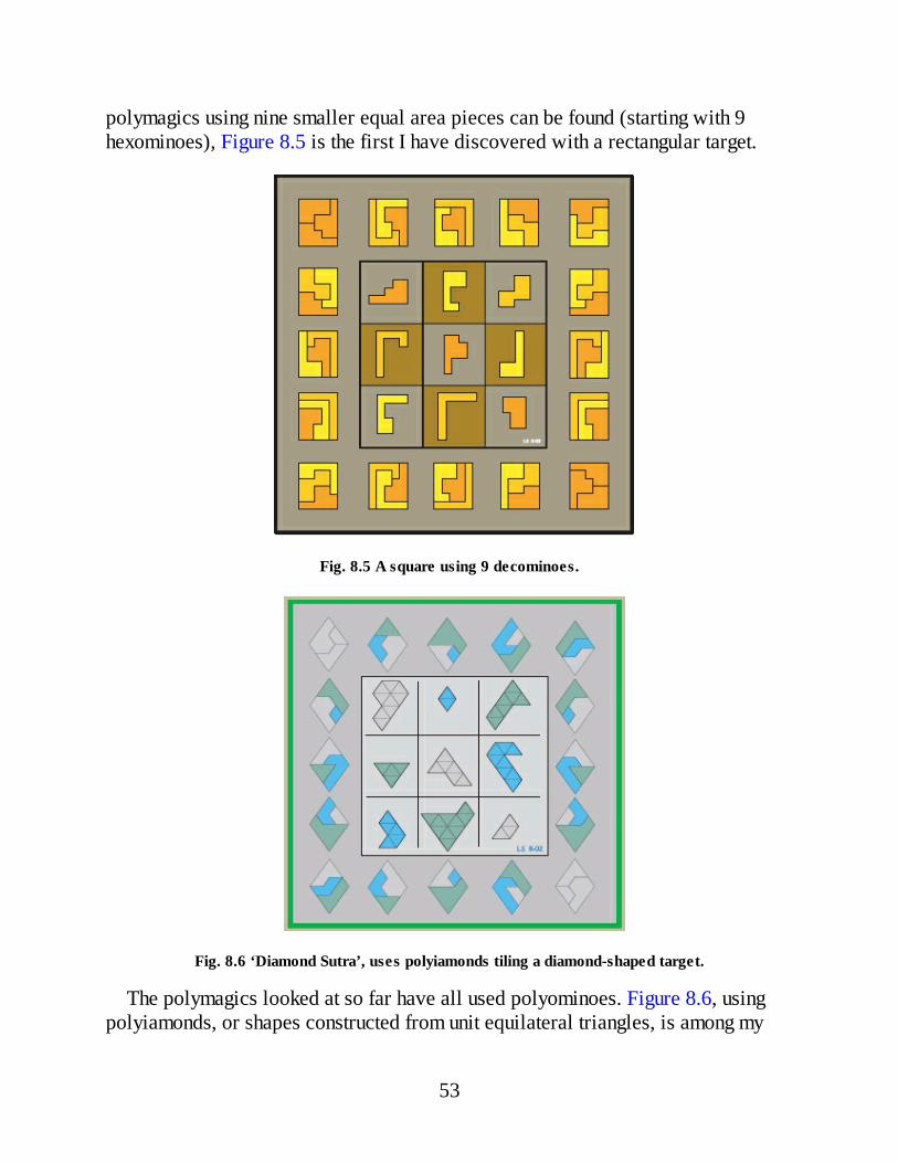
polymagics using nine smaller equal area pieces can be found (starting with 9hexominoes), Figure 8.5 is the first I have discovered with a rectangular target.

Fig. 8.5 A square using 9 decominoes.

Fig. 8.6 ‘Diamond Sutra’, uses polyiamonds tiling a diamond-shaped target.

The polymagics looked at so far have all used polyominoes. Figure 8.6, usingpolyiamonds, or shapes constructed from unit equilateral triangles, is among my

53

favourite finds. The target, here drawn at a reduced scale, is an equilateralparallelogram or diamond, while the piece sizes form a consective series, obtainedby adding 1 to the entries in the Lo shu.

Since the 9 pieces used here form three diamonds, the latter can be put togetherto form a regular hexagon. Now the area of the diamond is 18 units, and since thereare only eight ways in which three integers with a sum of 18 can be chosen from 2,3, . . . , 10, the targets shown in Figure 8.6 must account for every possiblediamond formable using three of these pieces. Three diamonds can be chosen fromamong the eight possibilities in (8/3) = 56 ways. Moreover, each diamond can bereflected about either or both of its diagonals so as to yield 4 possible orientations,with the result that any given triad of diamonds can be assembled in 4 × 4 × 4 = 64different ways so as to complete a distinct hexagon. In total there are thus 56 × 64= 3,584 distinct hexagons that can be created in this manner. Remarkably, however,the same pieces can be assembled to form a regular hexagon in many other ways,such as the following:

Fig. 8.7 A regular hexagon formed with the Diamond Sutra pieces.

In fact, computer investigation reveals an astonishing 17,213 distinct hexagonsthat can be constructed in this way, over and above the 3,584 already identified, atotal of 20,797 in all.

The title of Figure 8.6, Diamond Sutra, is perhaps a bit fanciful, but reflects myromantic view of geomagic squares as objects of contemplation (not to sayveneration). The same tendency reappears in the top center cover illustration andFigure 8.8, not merely in their titles, Magic Mandala I and II, but in theiroctagonal layout, an idea suggested by a Tibetan astrological diagram at the centreof which a 3×3 magic square is enclosed within a circle surrounded by eighttrigrams. The pieces used are again polyiamonds, with targets that are in both casesa regular hexagon. The key in Figure 8.9 identifies the target associated with eachrow, column, and diagonal. These are the only two solutions using polyiamondswith these sizes and same target shape, the corresponding area squares being inboth cases Latin squares. However, using nine pieces of size 4, 5, 6, . . . ,12, there

54

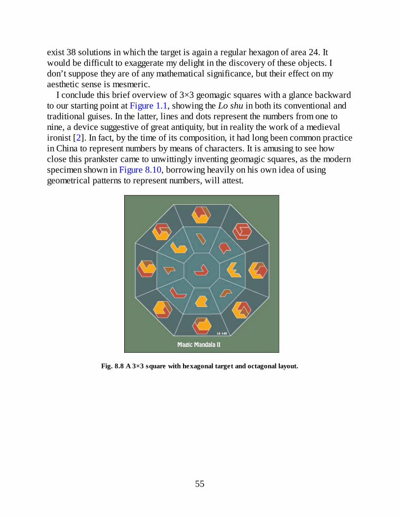
exist 38 solutions in which the target is again a regular hexagon of area 24. Itwould be difficult to exaggerate my delight in the discovery of these objects. Idon’t suppose they are of any mathematical significance, but their effect on myaesthetic sense is mesmeric.

I conclude this brief overview of 3×3 geomagic squares with a glance backwardto our starting point at Figure 1.1, showing the Lo shu in both its conventional andtraditional guises. In the latter, lines and dots represent the numbers from one tonine, a device suggestive of great antiquity, but in reality the work of a medievalironist [2]. In fact, by the time of its composition, it had long been common practicein China to represent numbers by means of characters. It is amusing to see howclose this prankster came to unwittingly inventing geomagic squares, as the modernspecimen shown in Figure 8.10, borrowing heavily on his own idea of usinggeometrical patterns to represent numbers, will attest.

Fig. 8.8 A 3×3 square with hexagonal target and octagonal layout.

55

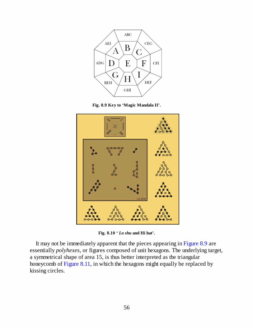
Fig. 8.9 Key to ‘Magic Mandala II’.

Fig. 8.10 ‘ Lo shu and Hi hat’.

It may not be immediately apparent that the pieces appearing in Figure 8.9 areessentially polyhexes, or figures composed of unit hexagons. The underlying target,a symmetrical shape of area 15, is thus better interpreted as the triangularhoneycomb of Figure 8.11, in which the hexagons might equally be replaced bykissing circles.

56

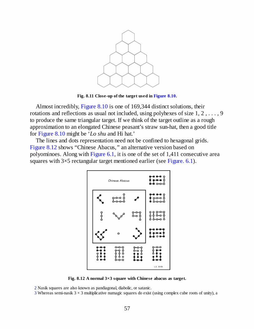
Fig. 8.11 Close-up of the target used in Figure 8.10.

Almost incredibly, Figure 8.10 is one of 169,344 distinct solutions, theirrotations and reflections as usual not included, using polyhexes of size 1, 2 , . . . , 9to produce the same triangular target. If we think of the target outline as a roughapproximation to an elongated Chinese peasant’s straw sun-hat, then a good titlefor Figure 8.10 might be ‘Lo shu and Hi hat.’

The lines and dots representation need not be confined to hexagonal grids.Figure 8.12 shows “Chinese Abacus,” an alternative version based onpolyominoes. Along with Figure 6.1, it is one of the set of 1,411 consecutive areasquares with 3×5 rectangular target mentioned earlier (see Figure. 6.1).

Fig. 8.12 A normal 3×3 square with Chinese abacus as target.

2 Nasik squares are also known as pandiagonal, diabolic, or satanic.3 Whereas semi-nasik 3 × 3 multiplicative numagic squares do exist (using complex cube roots of unity), a

57

fact nowhere previously recorded in the literature, so far as I am aware.4 A detailed discussion of fertility can be found in my article ‘New Advances with 4×4 Magic Squares’,

which is included as Appendix III.

58

Part II

Geomagic Squares of 4×4God invented the integers; everything else is the work of mantissae.

9 Geo-Latin Squares

Small is beautiful, yet the very compactness of 3×3 squares makes for stringentinternal constraints that severely delimit the solutions possible. Order-4 squaresare less tightly knit, for which reason they are more numerous, as well as richer invariety. Specimens were sought in the same ways as hitherto: (1) computersearches for polymagic types, and (2) hand constructions using algebraic formulaeas templates. In comparing squares brought to light by the two methods, at first, thefinds of the computer seem to outshine those of the pencil. In the sequel, however,the template technique yields results that exceed every expectation.

Unlike order-3, for which Lucas’s square offers the only candidate, there exists aplethora of non-trivial 4×4 formulae that may be used as templates. The latter arenot general formulae, but rather generalizations of certain subsets or special typesof 4×4 numerical magic squares. The mathematical properties of these subsets neednot concern us here, our interest lying solely in the use of these algebraic squaresfor designing 2-D magic squares. Many such formulae are based on Latin squares.

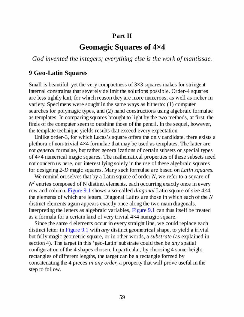
We remind ourselves that by a Latin square of order N, we refer to a square ofN2 entries composed of N distinct elements, each occurring exactly once in everyrow and column. Figure 9.1 shows a so-called diagonal Latin square of size 4×4,the elements of which are letters. Diagonal Latins are those in which each of the Ndistinct elements again appears exactly once along the two main diagonals.Interpreting the letters as algebraic variables, Figure 9.1 can thus itself be treatedas a formula for a certain kind of very trivial 4×4 numagic square.

Since the same 4 elements occur in every straight line, we could replace eachdistinct letter in Figure 9.1 with any distinct geometrical shape, to yield a trivialbut fully magic geometric square, or in other words, a substrate (as explained insection 4). The target in this ‘geo-Latin’ substrate could then be any spatialconfiguration of the 4 shapes chosen. In particular, by choosing 4 same-heightrectangles of different lengths, the target can be a rectangle formed byconcatenating the 4 pieces in any order, a property that will prove useful in thestep to follow.

59

Fig. 9.1 A 4×4 diagonal Latin square.

As in detrivializing 3×3 substrates, a pattern of keys and keyholes is now neededthat will modify these geo-Latin pieces so as to yield 16 distinct shapes. This isanalogous to the task of looking for a pattern of +x ’s and –x ’s that could be addedto the Latin square so as to yield 16 distinct entries, while preserving a constantsum in every row, column, and diagonal. However, the fact that A, B, C. and Deach occur 4 times means that at least two distinct variables will be needed. A fewtrials with pencil and paper came up with the pattern of a´s and b s in Figure 9.2,which can thus be interpreted as a formula for a certain subset of non-trivialnumagic squares. The advantage of choosing pieces that can tile the target in anyorder now means that pieces assigned keys will be able to marry with thoseassigned matching keyholes, irrespective of the particular detrivializing patternchosen.

Fig. 9.2 Every entry is unique.

Let a be a small half-circle and b a small isoceles triangle. Then replacing A, B,C, D with same-height rectangles of length 1, 2, 3, 4, respectively, we produce thegeomagic square in Figure 9.3, the target of which (not shown) is a rectangle oflength 1+2 + 3 + 4 = 10.

60

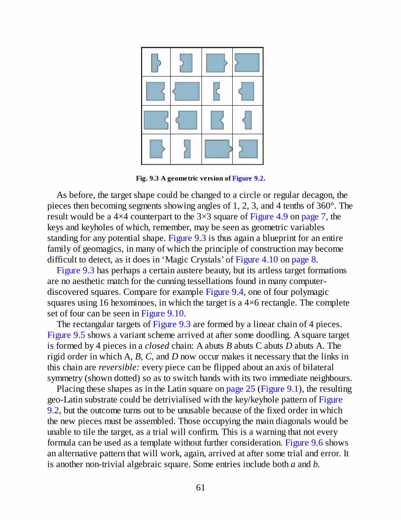
Fig. 9.3 A geometric version of Figure 9.2.

As before, the target shape could be changed to a circle or regular decagon, thepieces then becoming segments showing angles of 1, 2, 3, and 4 tenths of 360°. Theresult would be a 4×4 counterpart to the 3×3 square of Figure 4.9 on page 7, thekeys and keyholes of which, remember, may be seen as geometric variablesstanding for any potential shape. Figure 9.3 is thus again a blueprint for an entirefamily of geomagics, in many of which the principle of construction may becomedifficult to detect, as it does in ‘Magic Crystals’ of Figure 4.10 on page 8.

Figure 9.3 has perhaps a certain austere beauty, but its artless target formationsare no aesthetic match for the cunning tessellations found in many computer-discovered squares. Compare for example Figure 9.4, one of four polymagicsquares using 16 hexominoes, in which the target is a 4×6 rectangle. The completeset of four can be seen in Figure 9.10.

The rectangular targets of Figure 9.3 are formed by a linear chain of 4 pieces.Figure 9.5 shows a variant scheme arrived at after some doodling. A square targetis formed by 4 pieces in a closed chain: A abuts B abuts C abuts D abuts A. Therigid order in which A, B, C, and D now occur makes it necessary that the links inthis chain are reversible: every piece can be flipped about an axis of bilateralsymmetry (shown dotted) so as to switch hands with its two immediate neighbours.

Placing these shapes as in the Latin square on page 25 (Figure 9.1), the resultinggeo-Latin substrate could be detrivialised with the key/keyhole pattern of Figure9.2, but the outcome turns out to be unusable because of the fixed order in whichthe new pieces must be assembled. Those occupying the main diagonals would beunable to tile the target, as a trial will confirm. This is a warning that not everyformula can be used as a template without further consideration. Figure 9.6 showsan alternative pattern that will work, again, arrived at after some trial and error. Itis another non-trivial algebraic square. Some entries include both a and b.

61

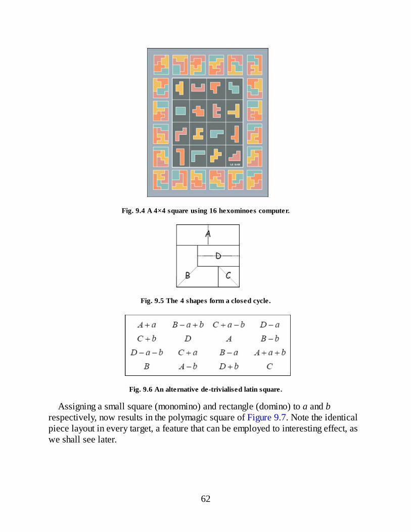
Fig. 9.4 A 4×4 square using 16 hexominoes computer.

Fig. 9.5 The 4 shapes form a closed cycle.

Fig. 9.6 An alternative de-trivialised latin square.

Assigning a small square (monomino) and rectangle (domino) to a and brespectively, now results in the polymagic square of Figure 9.7. Note the identicalpiece layout in every target, a feature that can be employed to interesting effect, aswe shall see later.

62

Fig. 9.7 A geometrical version of Figure 9.6.

Again, the visual logic of Figure 9.7 may be compelling, but the unvarying targetassembly is unsatisying in comparison with Figure 9.8, for example, which isanother computer-discovered polymagic square.

Here, the desire for a square target dictated the choice of piece sizes. Everymagic line contains three hexominoes and one heptomino. 3 × 6 + 7 = 5 × 5, thearea of the square target. But things can work the other way around. In an earlierchapter it was noted that there exist no 3×3 geomagics using nine pentominoes.Figure 9.9 goes some way to make up for this injustice. Here, four tetrominoescombine with the full set of twelve pentominoes to provide the 16 piecesemployed. It is a matter of regret that, despite every attempt to discover a morepleasing result, the target is an incomplete rectangle.

10 4×4 Nasiks

The template method can also be used to create a 4×4 nasik square. Glancing againat the Latin square in Figure 9.1, we see that for the broken diagonals to becomemagic would require 2A + 2B = 2C + 2D = A + B + C + D, or A + B = C + D.Rearranging the piece lengths in Figure 9.3 to A = 1, B = 4, C = 2, and D = 3,which achieves this, would, therefore, result in a 4×4 nasik square, provided a newkey/ keyhole pattern can be found that will again detrivialize the Latin squarewithout destroying its nasik property, as both of the previously used patterns inFigures 9.2 and 9.6 in fact do. Such nasik-preserving patterns can indeed be found,but in every case tried, the resulting set of pieces were unable to tile the target.Two keys on one piece cannot marry with their corresponding keyholes because

63

both of the latter turn out to occupy another single piece.

Fig. 9.8 A computer-discovered 4×4 square.

Fig. 9.9 A 4×4 square containing all twelve pentominoes.

64

Fig. 9.10 Four squares using 16 hexominoes and 4×6 target.

There exist however Latin squares other than Figure 9.1. Figure 10.1 shows anon-diagonal 4×4 Latin square.

Fig. 10.1 A non-diagonal Latin square

Inspection shows that this becomes nasik when A + D = B + C, or D = B + C –A, the magic sum then becoming 2B + 2C. Figure 10.2 shows a pattern of variablesthat detrivialises this square without interfering with its nasik property: every row,column, and diagonal sums to zero.

Fig. 10.2 Every row, column, and diagonal sims to zero.

65

Combining the nasik Latin with this pattern then yields Figure 10.3, a non-trivialalgebraic square different again to Figures 9.2 or 9.6:

A geometrical analog of this is seen in Figure 10.4, in which A, B, and C arerepresented by same-height rectangles of length 1,3, and 2, respectively, with a asmall half-circle and b a half-square. The target is a rectangle of length 2B + 2C =10. The piece labels A, B, . . ., P must not be confused with the variables A, B, Cin Figure 10.3.

Fig. 10.3

Fig. 10.4

66

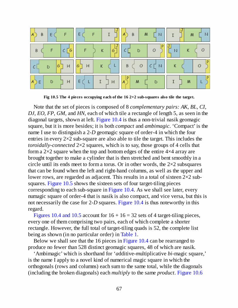
Fig 10.5 The 4 pieces occupying each of the 16 2×2 sub-squares also tile the target.

Note that the set of pieces is composed of 8 complementary pairs: AK, BL, CI,DJ, EO, FP, GM, and HN, each of which tile a rectangle of length 5, as seen in thediagonal targets, shown at left. Figure 10.4 is thus a non-trivial nasik geomagicsquare, but it is more besides; it is both compact and ambimagic. ‘Compact’ is thename I use to distinguish a 2-D geomagic square of order-4 in which the fourentries in every 2×2 sub-square are also able to tile the target. This includes thetoroidally-connected 2×2 squares, which is to say, those groups of 4 cells thatform a 2×2 square when the top and bottom edges of the entire 4×4 array arebrought together to make a cylinder that is then stretched and bent smoothly in acircle until its ends meet to form a torus. Or in other words, the 2×2 subsquaresthat can be found when the left and right-hand columns, as well as the upper andlower rows, are regarded as adjacent. This results in a total of sixteen 2×2 sub-squares. Figure 10.5 shows the sixteen sets of four target-tiling piecescorresponding to each sub-square in Figure 10.4. As we shall see later, everynumagic square of order-4 that is nasik is also compact, and vice versa, but this isnot necessarily the case for 2-D squares. Figure 10.4 is thus noteworthy in thisregard.

Figures 10.4 and 10.5 account for 16 + 16 = 32 sets of 4 target-tiling pieces,every one of them comprising two pairs, each of which complete a shorterrectangle. However, the full total of target-tiling quads is 52, the complete listbeing as shown (in no particular order) in Table 1.

Below we shall see that the 16 pieces in Figure 10.4 can be rearranged toproduce no fewer than 528 distinct geomagic squares, 48 of which are nasik.

‘Ambimagic’ which is shorthand for ‘additive-multiplicative bi-magic square,’is the name I apply to a novel kind of numerical magic square in which theorthogonals (rows and columns) each sum to the same total, while the diagonals(including the broken diagonals) each multiply to the same product. Figure 10.6

67

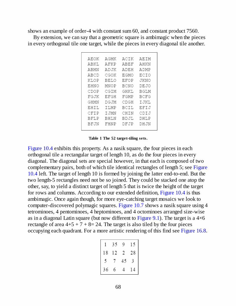
shows an example of order-4 with constant sum 60, and constant product 7560.By extension, we can say that a geometric square is ambimagic when the pieces

in every orthogonal tile one target, while the pieces in every diagonal tile another.

Table 1 The 52 target-tiling sets.

Figure 10.4 exhibits this property. As a nasik square, the four pieces in eachorthogonal tile a rectangular target of length 10, as do the four pieces in everydiagonal. The diagonal sets are special however, in that each is composed of twocomplementary pairs, both of which tile identical rectangles of length 5; see Figure10.4 left. The target of length 10 is formed by joining the latter end-to-end. But thetwo length-5 rectangles need not be so joined. They could be stacked one atop theother, say, to yield a distinct target of length 5 that is twice the height of the targetfor rows and columns. According to our extended definition, Figure 10.4 is thusambimagic. Once again though, for more eye-catching target mosaics we look tocomputer-discovered polymagic squares. Figure 10.7 shows a nasik square using 4tetrominoes, 4 pentominoes, 4 heptominoes, and 4 octominoes arranged size-wiseas in a diagonal Latin square (but now different to Figure 9.1). The target is a 4×6rectangle of area 4+5 + 7 + 8= 24. The target is also tiled by the four piecesoccupying each quadrant. For a more artistic rendering of this find see Figure 16.8.

68

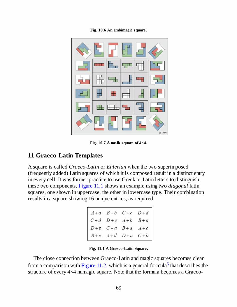
Fig. 10.6 An ambimagic square.

Fig. 10.7 A nasik square of 4×4.

11 Graeco-Latin Templates

A square is called Graeco-Latin or Eulerian when the two superimposed(frequently added) Latin squares of which it is composed result in a distinct entryin every cell. It was former practice to use Greek or Latin letters to distinguishthese two components. Figure 11.1 shows an example using two diagonal latinsquares, one shown in uppercase, the other in lowercase type. Their combinationresults in a square showing 16 unique entries, as required.

Fig. 11.1 A Graeco-Latin Square.

The close connection between Graeco-Latin and magic squares becomes clearfrom a comparison with Figure 11.2, which is a general formula5 that describes thestructure of every 4×4 numagic square. Note that the formula becomes a Graeco-

69

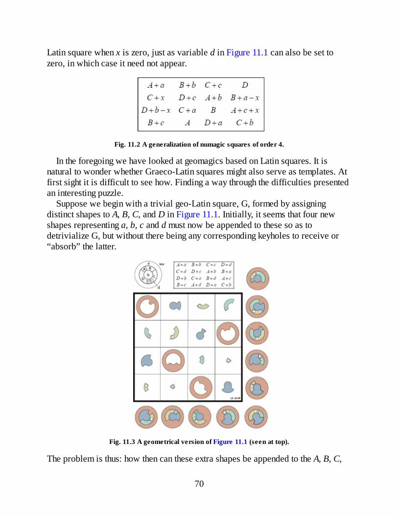
Latin square when x is zero, just as variable d in Figure 11.1 can also be set tozero, in which case it need not appear.

Fig. 11.2 A generalization of numagic squares of order 4.

In the foregoing we have looked at geomagics based on Latin squares. It isnatural to wonder whether Graeco-Latin squares might also serve as templates. Atfirst sight it is difficult to see how. Finding a way through the difficulties presentedan interesting puzzle.

Suppose we begin with a trivial geo-Latin square, G, formed by assigningdistinct shapes to A, B, C, and D in Figure 11.1. Initially, it seems that four newshapes representing a, b, c and d must now be appended to these so as todetrivialize G, but without there being any corresponding keyholes to receive or“absorb” the latter.

Fig. 11.3 A geometrical version of Figure 11.1 (seen at top).

The problem is thus: how then can these extra shapes be appended to the A, B, C,

70

and D pieces so that the square remains geomagic?We shall look at two solutions, their initial geo-Latin squares forming circular

and (roughly) rectangular targets, respectively. In the first case, the final form of thetarget remains a circle, in the second, we are able to choose virtually any shapedesired.

Figure 11.3 shows a geo-Eulerian square in which the target is a circular discshowing two adjacent holes, one square, and one circular. A, B, C, and D arerepresented by annular segments subtending arcs of 1, 2, 3, and 4 tenths of 360°, toresult in a geo-Latin square in which the 4 pieces can be assembled in any order tocomplete an annular target. This is the ring sandwiched between a and b, the outerring and the inner circle, as seen in the target key shown at top left in Figure 11.3.

The problem of appending magic-preserving keys-without-keyholes to thesepieces is then solved by means of two separate devices:

(1) By choosing key-shapes with rotational symmetry, a property that allows them to be appended to the fourdifferent annular segments so as to preserve target circularity. These are a and b, the outer ring and innercircle.

(2) By interpreting two of the Eulerian elements as negative or excised areas. That is, the second Latin square(using small letters) is treated as shown in Figure 11.4, in which –c and –d correspond to the small circularand square holes, respectively.

Fig. 11.4 A latin square with negative entries.

The latter serve to detrivialize the annular segments, whose ability to beassembled in different orderings means that these two holes can always bearranged to appear in a fixed relation to each other in every target. Note that –c and–d are not accompanied by their positive counterparts, c and d. This concludes ourglance at the circular target case.

Figure 11.5 shows a quite different geo-Eulerian square that is based on a geo-latin square using rectangular rather than annular pieces. The Eulerian template isnow Figure 11.6, which is Figure 11.1 with d = –c, a trick that provides any keyrepresented by c with a matching keyhole, and thus overcomes one difficulty at astroke. As in previous cases, A, B, C, and D are now replaced by same-heightrectangles of length 1 (red), 2 (green), 3 (blue), and 4 (yellow), the target formedby these being a rectangle of length 10. Again, the ability to concatenate these

71

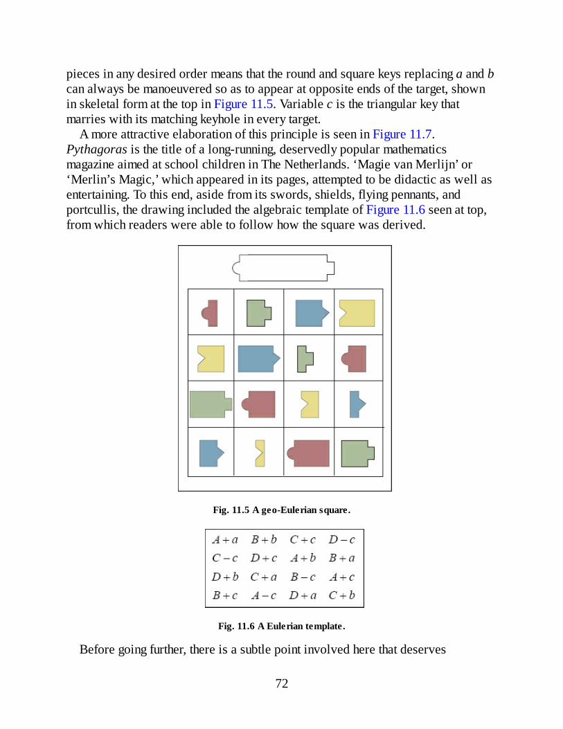
pieces in any desired order means that the round and square keys replacing a and bcan always be manoeuvered so as to appear at opposite ends of the target, shownin skeletal form at the top in Figure 11.5. Variable c is the triangular key thatmarries with its matching keyhole in every target.

A more attractive elaboration of this principle is seen in Figure 11.7.Pythagoras is the title of a long-running, deservedly popular mathematicsmagazine aimed at school children in The Netherlands. ‘Magie van Merlijn’ or‘Merlin’s Magic,’ which appeared in its pages, attempted to be didactic as well asentertaining. To this end, aside from its swords, shields, flying pennants, andportcullis, the drawing included the algebraic template of Figure 11.6 seen at top,from which readers were able to follow how the square was derived.

Fig. 11.5 A geo-Eulerian square.

Fig. 11.6 A Eulerian template.

Before going further, there is a subtle point involved here that deserves

72

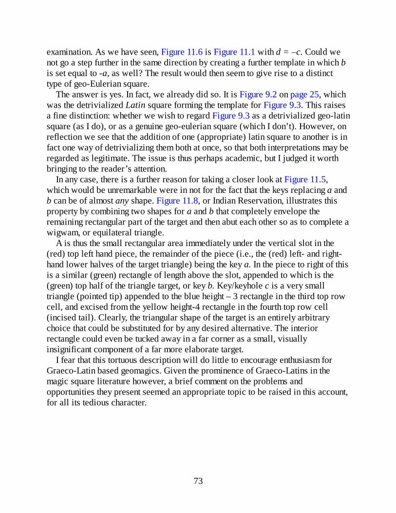
examination. As we have seen, Figure 11.6 is Figure 11.1 with d = –c. Could wenot go a step further in the same direction by creating a further template in which bis set equal to -a, as well? The result would then seem to give rise to a distincttype of geo-Eulerian square.

The answer is yes. In fact, we already did so. It is Figure 9.2 on page 25, whichwas the detrivialized Latin square forming the template for Figure 9.3. This raisesa fine distinction: whether we wish to regard Figure 9.3 as a detrivialized geo-latinsquare (as I do), or as a genuine geo-eulerian square (which I don’t). However, onreflection we see that the addition of one (appropriate) latin square to another is infact one way of detrivializing them both at once, so that both interpretations may beregarded as legitimate. The issue is thus perhaps academic, but I judged it worthbringing to the reader’s attention.

In any case, there is a further reason for taking a closer look at Figure 11.5,which would be unremarkable were in not for the fact that the keys replacing a andb can be of almost any shape. Figure 11.8, or Indian Reservation, illustrates thisproperty by combining two shapes for a and b that completely envelope theremaining rectangular part of the target and then abut each other so as to complete awigwam, or equilateral triangle.

A is thus the small rectangular area immediately under the vertical slot in the(red) top left hand piece, the remainder of the piece (i.e., the (red) left- and right-hand lower halves of the target triangle) being the key a. In the piece to right of thisis a similar (green) rectangle of length above the slot, appended to which is the(green) top half of the triangle target, or key b. Key/keyhole c is a very smalltriangle (pointed tip) appended to the blue height – 3 rectangle in the third top rowcell, and excised from the yellow height-4 rectangle in the fourth top row cell(incised tail). Clearly, the triangular shape of the target is an entirely arbitrarychoice that could be substituted for by any desired alternative. The interiorrectangle could even be tucked away in a far corner as a small, visuallyinsignificant component of a far more elaborate target.

I fear that this tortuous description will do little to encourage enthusiasm forGraeco-Latin based geomagics. Given the prominence of Graeco-Latins in themagic square literature however, a brief comment on the problems andopportunities they present seemed an appropriate topic to be raised in this account,for all its tedious character.

73

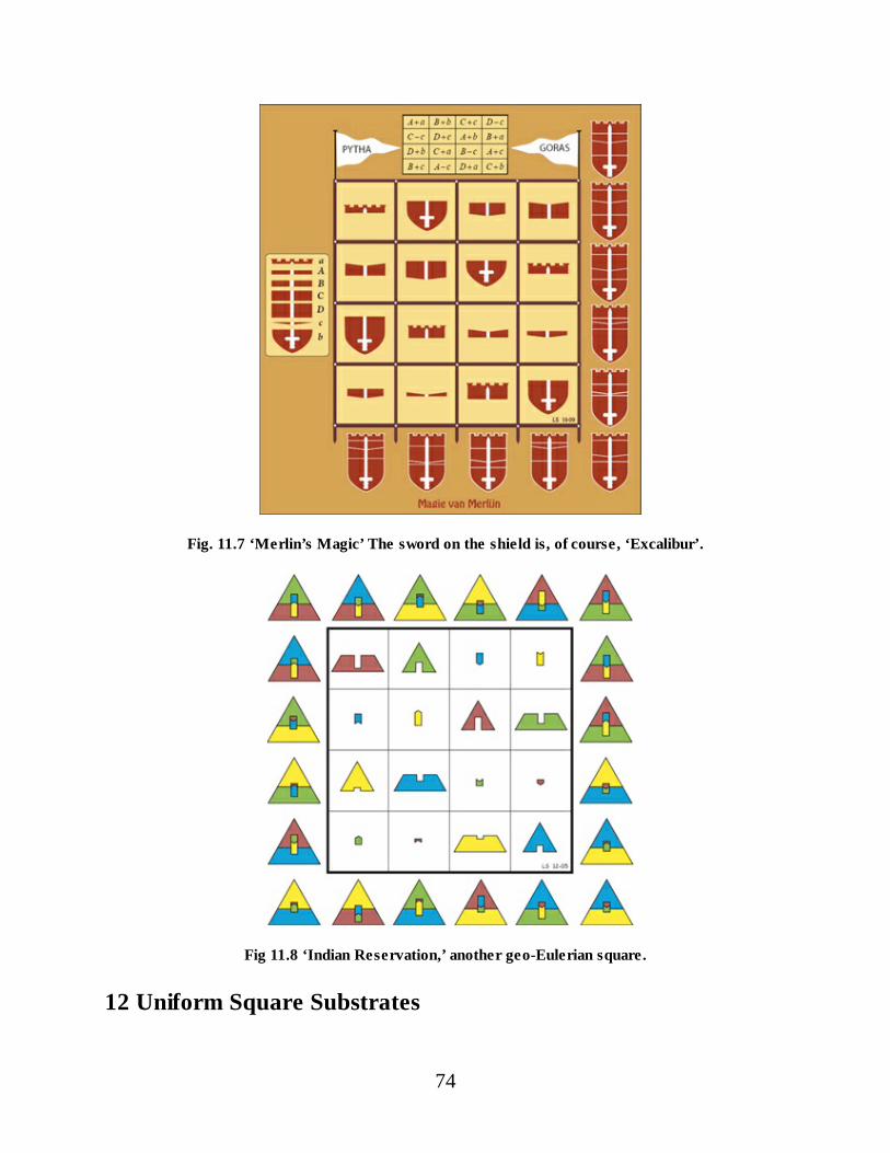
Fig. 11.7 ‘Merlin’s Magic’ The sword on the shield is, of course, ‘Excalibur’.

Fig 11.8 ‘Indian Reservation,’ another geo-Eulerian square.

12 Uniform Square Substrates

74

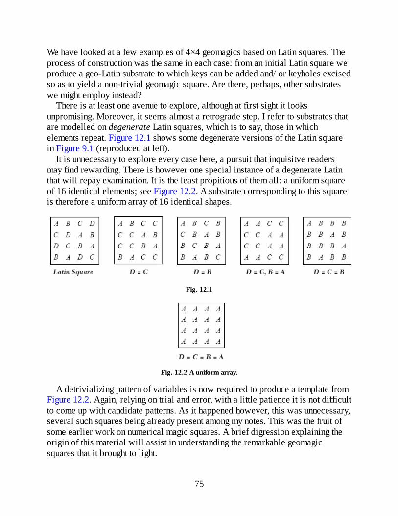
We have looked at a few examples of 4×4 geomagics based on Latin squares. Theprocess of construction was the same in each case: from an initial Latin square weproduce a geo-Latin substrate to which keys can be added and/ or keyholes excisedso as to yield a non-trivial geomagic square. Are there, perhaps, other substrateswe might employ instead?

There is at least one avenue to explore, although at first sight it looksunpromising. Moreover, it seems almost a retrograde step. I refer to substrates thatare modelled on degenerate Latin squares, which is to say, those in whichelements repeat. Figure 12.1 shows some degenerate versions of the Latin squarein Figure 9.1 (reproduced at left).

It is unnecessary to explore every case here, a pursuit that inquisitve readersmay find rewarding. There is however one special instance of a degenerate Latinthat will repay examination. It is the least propitious of them all: a uniform squareof 16 identical elements; see Figure 12.2. A substrate corresponding to this squareis therefore a uniform array of 16 identical shapes.

Fig. 12.1

Fig. 12.2 A uniform array.

A detrivializing pattern of variables is now required to produce a template fromFigure 12.2. Again, relying on trial and error, with a little patience it is not difficultto come up with candidate patterns. As it happened however, this was unnecessary,several such squares being already present among my notes. This was the fruit ofsome earlier work on numerical magic squares. A brief digression explaining theorigin of this material will assist in understanding the remarkable geomagicsquares that it brought to light.

75

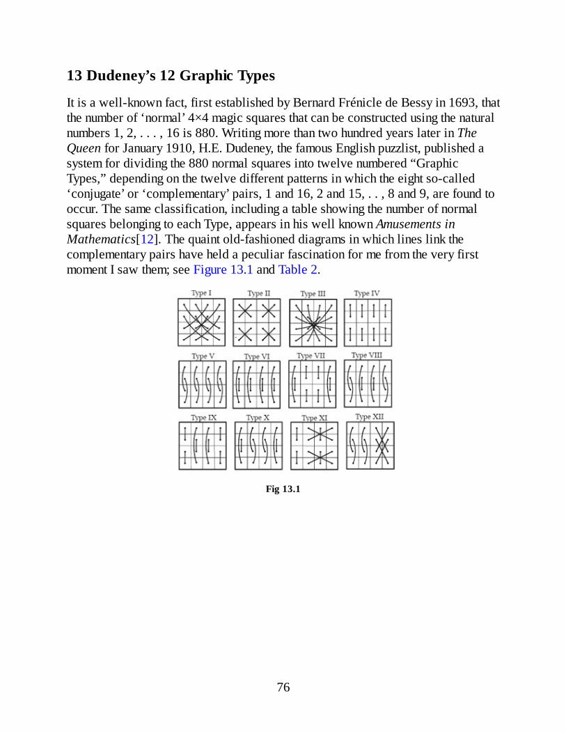
13 Dudeney’s 12 Graphic Types

It is a well-known fact, first established by Bernard Frénicle de Bessy in 1693, thatthe number of ‘normal’ 4×4 magic squares that can be constructed using the naturalnumbers 1, 2, . . . , 16 is 880. Writing more than two hundred years later in TheQueen for January 1910, H.E. Dudeney, the famous English puzzlist, published asystem for dividing the 880 normal squares into twelve numbered “GraphicTypes,” depending on the twelve different patterns in which the eight so-called‘conjugate’ or ‘complementary’ pairs, 1 and 16, 2 and 15, . . , 8 and 9, are found tooccur. The same classification, including a table showing the number of normalsquares belonging to each Type, appears in his well known Amusements inMathematics[12]. The quaint old-fashioned diagrams in which lines link thecomplementary pairs have held a peculiar fascination for me from the very firstmoment I saw them; see Figure 13.1 and Table 2.

Fig 13.1

76

Table 2

77

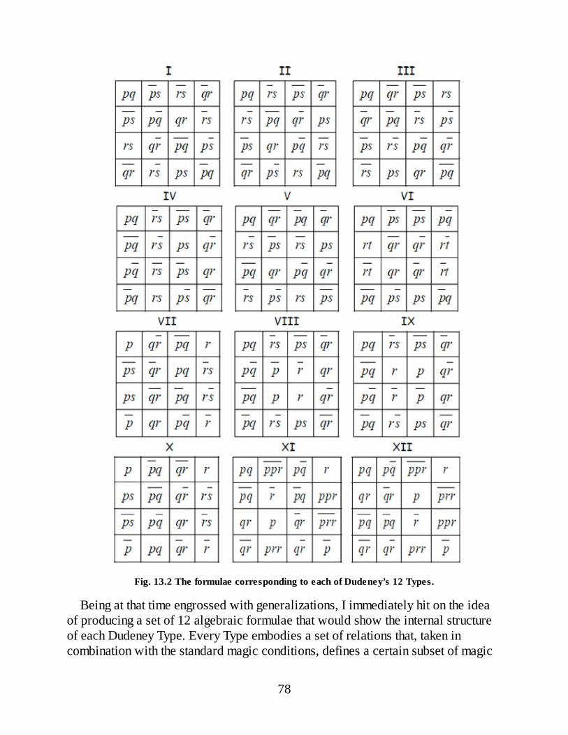
Fig. 13.2 The formulae corresponding to each of Dudeney’s 12 Types.

Being at that time engrossed with generalizations, I immediately hit on the ideaof producing a set of 12 algebraic formulae that would show the internal structureof each Dudeney Type. Every Type embodies a set of relations that, taken incombination with the standard magic conditions, defines a certain subset of magic

78

squares whose characteristics can be captured in a restricted or non-generalformula. The result of this project, written up more fully in an unpublished article,“Magic Formulae,” 6 dated 1980, is reproduced in Figure 13.2.

Compression is achieved by writing ab for a+b, and for –a, the magic sum ineach case being zero. Adding an appropriate constant to each cell will then yield asquare having any desired magic sum. More generally, adding the same variable,say A, to every cell in, for example, the formula for Type I, results in Figure 13.3,which is thus a non-abbreviated generalization of all Type I squares, includingthose with a non-zero magic sum.

Fig. 13.3 A formula for Type I squares.

This returns us to our starting point, for Figure 13.3 is a detrivialized version ofthe uniform square in Figure 12.2, the magic sum being 4A. Note that its six brokendiagonals each sum to 4A, also. This is because Dudeney’s classification “Type I,”although at first sight unrelated, is, in fact, indistinguishable from the classification“nasik”. Specifically, it can be shown that, normal or not, every numerical 4×4nasik square is necessarily composed of 8 complementary pairs distributed asshown in Type I, and vice versa, the sum of each pair being 2A, or half the magicconstant. In the same way, it can be shown that for numerical magic squares ingeneral, Type I = nasik = compact, a relation that, as we shall see, does not alwayshold for 2-D geomagics.

Fig. 14.1 A generalization of 4×4 nasik squares.

Here then was the first of twelve ready-made templates that were still there atthe back of my mind some 25 years later, by which time two-dimensional squareshad become the focus of interest, with numerical magic squares now occupying a

79

back seat. A few further remarks on the background to these 12 formulae willexplain my curiosity to examine a geomagic square based on Figure 13.3.

14 The 12 Formulae

It is important to realize that the expression of a generalization can take widelydiffering forms. Figure 13.3, for example, is simply an alternative way of writingFigure 10.3 on page 30, both of them being formulae that describe the structure of4×4 nasik or Type I squares. Figure 14.1 shows yet a further alternative7. Thesethree algebraic squares are thus mathematically synonymous, or isomorphic, beingsimply different expressions of the same set of intercellular relations. In short,formulae that are mathematically identical can differ enormously in outwardappearance. Nevertheless, as we have seen, when it comes to using theseequivalent formulae as templates, not only are the geomagic squares they give riseto quite different, but their magical properties can even differ from those of theirparent formulae.

Likewise, any of the 12 formulae of Figure 13.2 could appear in alternate guises,some of them more elegant than others. By ‘elegant’, I mean more visuallysymmetrical, as well as more condensed or economical in symbol appearances. Itwas with this in mind that these 12 squares were produced. That is to say, far frombeing simply calculated or deduced, they are the product of a gradual process ofrefinement based upon trial and error, the motive behind which was primarilyaesthetic, with the aim of culminating in an ideal, or canonical exemplar, for eachType. Candidate squares arrived at via this process then had to be tested forvalidity by comparing them for isomorphism with a standard formula, known to becorrect. As a magic-square buff hooked on symmetry, it pleased me to strivepatiently for the most elegant expression of each formula, even if the end result wasof no mathematical significance.

But as chance had it, this artistic impulse led to an incidental discovery of someinterest. For I came to notice that in certain cases the formulae for distinct Typescould be written using the same set of 16 algebraic terms. The effect of this insightprompted a more systematic analysis, the result of which was decisive for theoutcome. In particular, as inspection of Figure 13.2 will verify, the final version ofthe 12 formulae fall into four classes sharing identical entries:

Class 1 : Types I, II, III, IV, V, (and that subset of Type VI when t = s or-s)Class 2 : Type VI (excluding the above subset members)Class 3 : Types VII, VIII, IX, XClass 4 : Types XI, XII

80

Properly understood therefore, Figure 13.2 embodies a visual demonstration ofsomething that is otherwise far from obvious, namely, that the entries of a magicsquare belonging to a given Class may always be transposed so as to form a newsquare of different Type in the same Class. Given any square of Type I, forexample, its entries can be rearranged in the way shown by the formulae to producestill others of Types II, III, IV, V, and VI. How many can be formed in all?

As shown by Dudeney’s table in Figure 13.1, the numbers 1, 2, . . . , 16 can beplaced so as to produce 48 Type I squares. Dudeney arrived at this result byenumeration, which is to say, by counting squares. It wasn’t until 1938 that a paperby Rosser and Walker [13] gave a proof of the same result based upon group-theoretic arguments. This was an important advance, although the authors mighthave achieved more.

In fact, it is not difficult to extend Rosser and Walker’s result to the 16 algebraicterms in Figure 13.3 (or its isomorphic twin, Figure 10.3). That is, it can be shownthat the entries in Figure 13.3 (or 10.3) can be placed so as to yield 48 distinctType I squares. But as just explained, the entries of any Type I square can berearranged to produce still others of Types II - VI, the total for each again being thesame as that given in Dudeney’s table, with one exception: the total for Type VI isnot 304 but 192, a discrepancy that is accounted for by the fact that Type VI squarescan also be constructed using Class 2 entries as well as those of Class 1. Thus,adding these totals together shows that the entries in Figure 13.3 (or 10.3) can berearranged to produce 48 + 48 + 48 + 96 + 96 + 192 = 528 distinct magic squares,rotations and reflections not counted.

How, I wondered, would a geomagic square derived from Figure 13.3 differfrom that based on Fig 10.3? Would the resulting set of pieces exhibit similarproperties so as to yield 528 geomagic squares? How would the enhanced visualsymmetry of the new template reflect itself in the result?

15 A Type I Geomagic Square

Digging out an old copy of Magic Formulae, I pondered the template of Figure13.3. The variables p, q, r, s could be allotted four distinct shapes that wouldbecome keys and keyholes on the substrate pieces represented by A. But whatshape to assign the latter? And what shape should the target take? A little thoughtshowed that the presence of a double key/keyhole on each piece means that those inthe target must form a closed circuit, for an open chain would leave a key and akeyhole unmarried. This implied a circular or regular polygonal target. In the lattercase, if A = 1 the magic sum is 4, which suggested a regular 4-gon, otherwiseknown as a square. Now here was a promising start.

81

On analogy with the hexagonal target met with earlier, this square target couldnow be divided radially into 4 identical segments subtending angles of 360°÷ 4 =90°. Three possibilities present themselves, two of them yielding symmetricalpieces, shown at right in Figure 15.1.

Choosing the rightmost, the substrate pieces then become square-shaped, too.Assigning now 4 distinct shapes to p, q, r, and s, Figure 15.2 shows the geomagicsquare to emerge from these meditations. The four colors used, arranged in a Latinconfiguration, make it easier to follow the construction.

Fig. 15.1 Dividing a square into four similar pieces.

Here then was a nice looking geomagic square, but a glance shows that at leastone important property of its template is lacking. The four pieces occupying eachof the long broken diagonals, such as p + q, –r + s, –p – q, and r – s, will not tilethe target. The two key/keyholes on any one piece must marry with the twokeyhole/keys on another (its complement), which is obviously impossible. Hence,even though it is of Type I, this geometric magic square is not nasik.

In the realm of numerical magic squares a nasik square is always of Type I, anda Type I square is always nasik. Why should geomagics behave differently? It isbecause the combinative properties of numbers are not shared by geometricalforms. In the template technique we replace algebraic variables with geometricalshapes, a stratagem that owes more to abracadabra than it does to mathematics.Small wonder then if this dubious method occasionally leads to odd results. For, aswith my original square based on Lucas’s formula (Figure 2.4), there can be noguarantee that the pieces it yields are able to successfully tile the target, eventhough their combined area will be the one required.

Notwithstanding this nasik deficiency, Figure 15.2 retains most of the attributesof its template. In particular, it embraces many other quads of target-tiling piecesbesides those seen in the 10 targets depicted. The square is compact, for example,a property that entails a further 16 target-tiling quads. It is natural to wonder howmany there are in total.

The magic constant in the template is 4A. The sum of the 4 algebraic termscorresponding to any quad of target-tiling pieces must therefore be the same. Acomputer program that examined in turn every set of 4 distinct terms occurring in

82

the formula finds 52 that sum to 4A. In the nasik square of Figure 10.4, every one ofthese corresponds to a target-tiling piece set. But not all of these will work here.There are 8 ‘forbidden’ sets among the 52 whose corresponding pieces will not tilea square. They are those that consist of two complementary pairs having novariable in common, as shown in Figure 15.3.

It is easy to see why these sets will not tile the target in spite of possessing theappropriate area of 4A. In the geomagic square these 8 sets are to be foundoccupying (1) the 4 long broken diagonals and (2) the 4 corner cells of the fourembedded 3×3 squares. In the list of 52 target-tiling quads associated with Figure10.4 (Table 1, page 31) they are the sets AHKN, DEJO, CFIP, BGLM, ACIK,BDJL, EGMO, and FHNP. The full number of target-tiling piece sets in Figure15.2 is thus 52 – 8 = 44.

As discussed above, a more striking attribute of the template is that its 16algebraic terms (the Class-1 entries) can be rearranged so as to form new squaresof Types II, III, IV, V, and VI. Identical rearrangements of the 16 pieces in Figure15.2 will thus result in new geomagic squares, provided no forbidden set occupiesa row, column, or main diagonal, which would render the square non-magic. Acomputer program that generated all 528 squares in turn and then filtered out thelatter cases found 144 squares remaining. The 16 pieces in Figure 15.2 will thusyield 144 distinct geomagic squares distributed over Types I – VI, the totals foreach Type being as shown in Table 3.

83

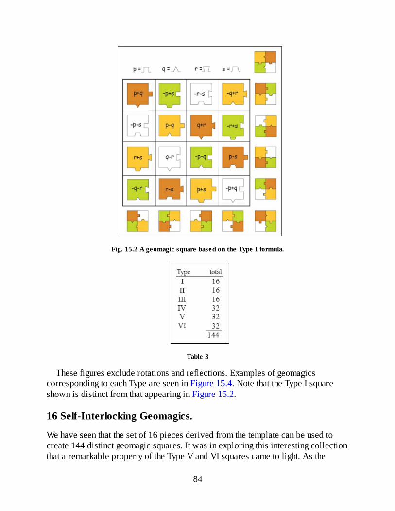
Fig. 15.2 A geomagic square based on the Type I formula.

Table 3

These figures exclude rotations and reflections. Examples of geomagicscorresponding to each Type are seen in Figure 15.4. Note that the Type I squareshown is distinct from that appearing in Figure 15.2.

16 Self-Interlocking Geomagics.

We have seen that the set of 16 pieces derived from the template can be used tocreate 144 distinct geomagic squares. It was in exploring this interesting collectionthat a remarkable property of the Type V and VI squares came to light. As the

84

examples in Figure 15.4 will show, the four pieces in each quadrant (e.g., p + q, –p + s, p – q, – p – s) can be squeezed together so as to form the target. These fourtarget squares can in turn be squeezed together so as to make a larger squarecombining every piece. The entire set of sixteen pieces can thus be implodedwithout any change in their orientation so as to form a single larger square. But thismeans that this larger square is itself a geomagic square of Type V or Type VI, theconstituent pieces of which happen to abut each other so as to form a regularquadrilateral, as seen in Figure 16.1.

Fig. 15.3 Every quad consists of two complementary pairs having no variable in common.

85

Fig. 15.4 Rearranging the pieces in Figure 15.2 to produce squares of Types I - VI.

Fig. 16.1 Two self-interlocking geomagic squares.

Thus far we have always thought of a geomagic square as an array of separatepieces, each occupying a distinct cell. Here we have an array of shapes whoseedges virtually coincide with, and thus define, their own cell boundaries. Thatthere exist many different sets of pieces that can be placed in a 4×4 array so as toyield a geomagic square is perhaps a surprising thing in itself. It would be counteda bonus if such a set of pieces could be rearranged in some way so as to tile asquare. In Figure 16.1, we are looking at a structure that achieves both of thesethings at once. For this reason, I call these geomagic squares “self-interlocking,”and there are 64 of them in all, 32 of Type V and 32 of Type VI, rotations andreflections not counted.

To put the above in perspective, recall that the algebraic template of Figure 13.3is merely an alternative expression of Figure 10.3, itself used as a template toconstruct the nasik square of Figure 10.4. So here we have two isomorphictemplates, the one leading to a nasik, and the other to a non-nasik geomagic square.This again illustrates the peculiar property of the template technique alreadyencountered, namely, that the geomagic square it yields is determined as much bythe algebraic structure described by the formula, as it is by the particular set ofexpressions in which the formula happens to be couched. It is perhaps thus nocoincidence that the “most elegant” formula has given rise to these aestheticallypleasing self-interlocking squares.

The keys and keyholes used to modify the pieces in Figure 16.1 are entirelyarbitrary in shape, which means that alternatives can be used. “Magic JigsawPuzzle” in Figure 16.2 shows a re-expression of the Type V square in Figure 16.1using shapes more appropriate to its title. Twenty of the 44 possible targetssurround the square to complete a pleasing symmetrical ensemble. Note that thecentral square really does make a jigsaw puzzle, in that viewers can be invited toreassemble the 16 pieces so as to form a new square. There are 64 solutions, everyone of them forming a distinct self-interlocking geomagic square. They are listed in

86

Table 4. One simple solution is to switch diametrically opposed quadrants.Curiously, the key and keyhole shapes used in ‘Magic Jigsaw Puzzle’ are more

obviously ‘arbitrary’ than their originals, making both squares equally suitable as ablue print for designing alternative versions of the same structure. Figure 16.3shows another interpretation of the Type V square in which the keys and keyholesare monominoes and dominoes, to result in pieces, here slightly separated fromeach other, that are polyominoes. In this case, all 44 targets are shown. Below weshall take a closer look at exactly how the shapes of the polyominoes are arrivedat.

Note that symmetries in the key/keyhole interlocks mean that the four columntargets can each be tiled in three different ways. In the left-hand column target, forexample, the top half of the target square formed by pieces A and E could beflipped about its vertical midline and still marry with M and I, as required.

There is an alternative way to represent polyominoes, which is by tracing pathsthat link the centres of their constituent square cells, as in the example using pieceA, shown in Figure 16.4.

Such paths can often be drawn in different ways. Depending on the polyomino,forks in the path may be demanded, as in the example shown. Applying a similarapproach to every piece in Figure 16.3 results, for example, in Figure 16.5, whichis reminiscent of so-called ‘space-filling curves’ as well as designs to be found inArabic art.

87

Fig. 16.2 Magic Jigsaw Puzzle.

88

Table 4. The 64 magic rearrangements of ‘Magic Jigsaw Puzzle.’

89

Fig. 16.3 An alternative interpretation of the Type-V formula.

Fig. 16.4 Representing polyominoes by tracing paths.

Figure 16.6 shows the same square but now using 4 different colors distributedas in a diagonal Latin square. The central square is surrounded by 20 of its 44targets. Here the title, ‘Spatial Fugue,’ was suggested by analogies with the fugalmusic of J.S. Bach. Harmonic alignments, both ‘horizontal’ and ‘vertical’ are thechief characteristic of counterpoint, the resultant pattern of sounds forming atemporal sequence that, in the case of the composer Bach, can truly be described as‘magic,’ both in its figurative, as well as its literal sense.

90

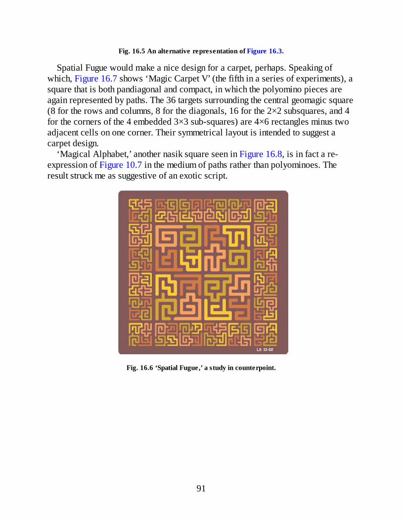
Fig. 16.5 An alternative representation of Figure 16.3.

Spatial Fugue would make a nice design for a carpet, perhaps. Speaking ofwhich, Figure 16.7 shows ‘Magic Carpet V’ (the fifth in a series of experiments), asquare that is both pandiagonal and compact, in which the polyomino pieces areagain represented by paths. The 36 targets surrounding the central geomagic square(8 for the rows and columns, 8 for the diagonals, 16 for the 2×2 subsquares, and 4for the corners of the 4 embedded 3×3 sub-squares) are 4×6 rectangles minus twoadjacent cells on one corner. Their symmetrical layout is intended to suggest acarpet design.

‘Magical Alphabet,’ another nasik square seen in Figure 16.8, is in fact a re-expression of Figure 10.7 in the medium of paths rather than polyominoes. Theresult struck me as suggestive of an exotic script.

Fig. 16.6 ‘Spatial Fugue,’ a study in counterpoint.

91

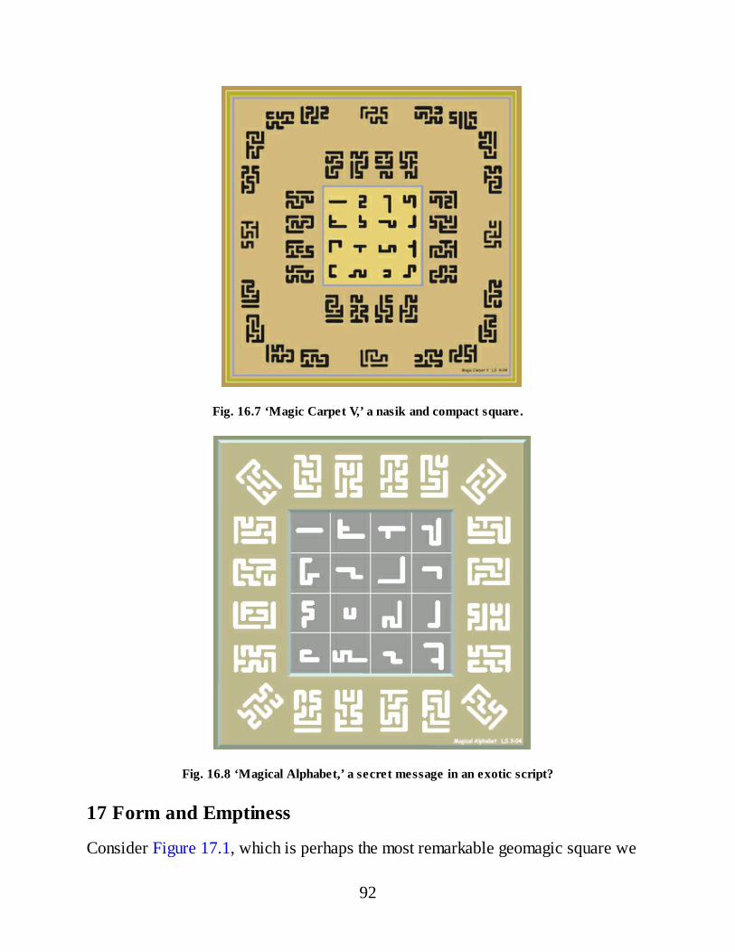
Fig. 16.7 ‘Magic Carpet V,’ a nasik and compact square.

Fig. 16.8 ‘Magical Alphabet,’ a secret message in an exotic script?

17 Form and Emptiness

Consider Figure 17.1, which is perhaps the most remarkable geomagic square we

92

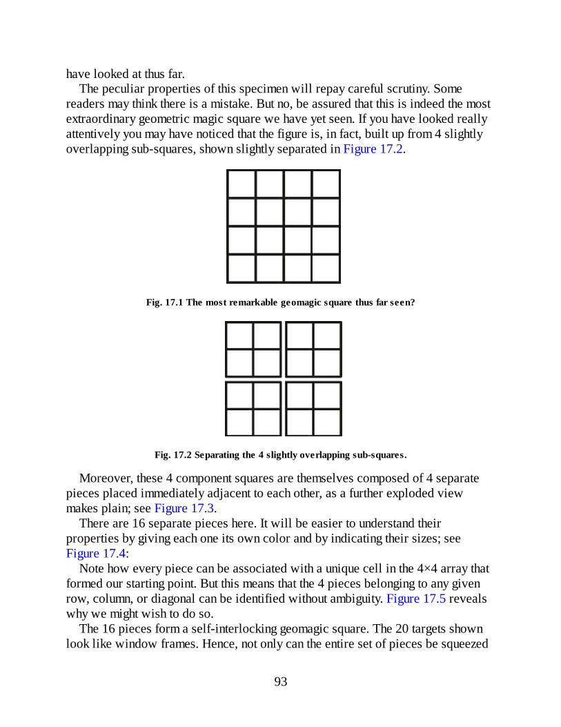
have looked at thus far.The peculiar properties of this specimen will repay careful scrutiny. Some

readers may think there is a mistake. But no, be assured that this is indeed the mostextraordinary geometric magic square we have yet seen. If you have looked reallyattentively you may have noticed that the figure is, in fact, built up from 4 slightlyoverlapping sub-squares, shown slightly separated in Figure 17.2.

Fig. 17.1 The most remarkable geomagic square thus far seen?

Fig. 17.2 Separating the 4 slightly overlapping sub-squares.

Moreover, these 4 component squares are themselves composed of 4 separatepieces placed immediately adjacent to each other, as a further exploded viewmakes plain; see Figure 17.3.

There are 16 separate pieces here. It will be easier to understand theirproperties by giving each one its own color and by indicating their sizes; seeFigure 17.4:

Note how every piece can be associated with a unique cell in the 4×4 array thatformed our starting point. But this means that the 4 pieces belonging to any givenrow, column, or diagonal can be identified without ambiguity. Figure 17.5 revealswhy we might wish to do so.

The 16 pieces form a self-interlocking geomagic square. The 20 targets shownlook like window frames. Hence, not only can the entire set of pieces be squeezed

93

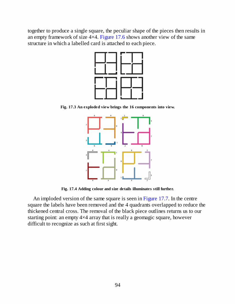
together to produce a single square, the peculiar shape of the pieces then results inan empty framework of size 4×4. Figure 17.6 shows another view of the samestructure in which a labelled card is attached to each piece.

Fig. 17.3 An exploded view brings the 16 components into view.

Fig. 17.4 Adding colour and size details illuminates still further.

An imploded version of the same square is seen in Figure 17.7. In the centresquare the labels have been removed and the 4 quadrants overlapped to reduce thethickened central cross. The removal of the black piece outlines returns us to ourstarting point: an empty 4×4 array that is really a geomagic square, howeverdifficult to recognize as such at first sight.

94

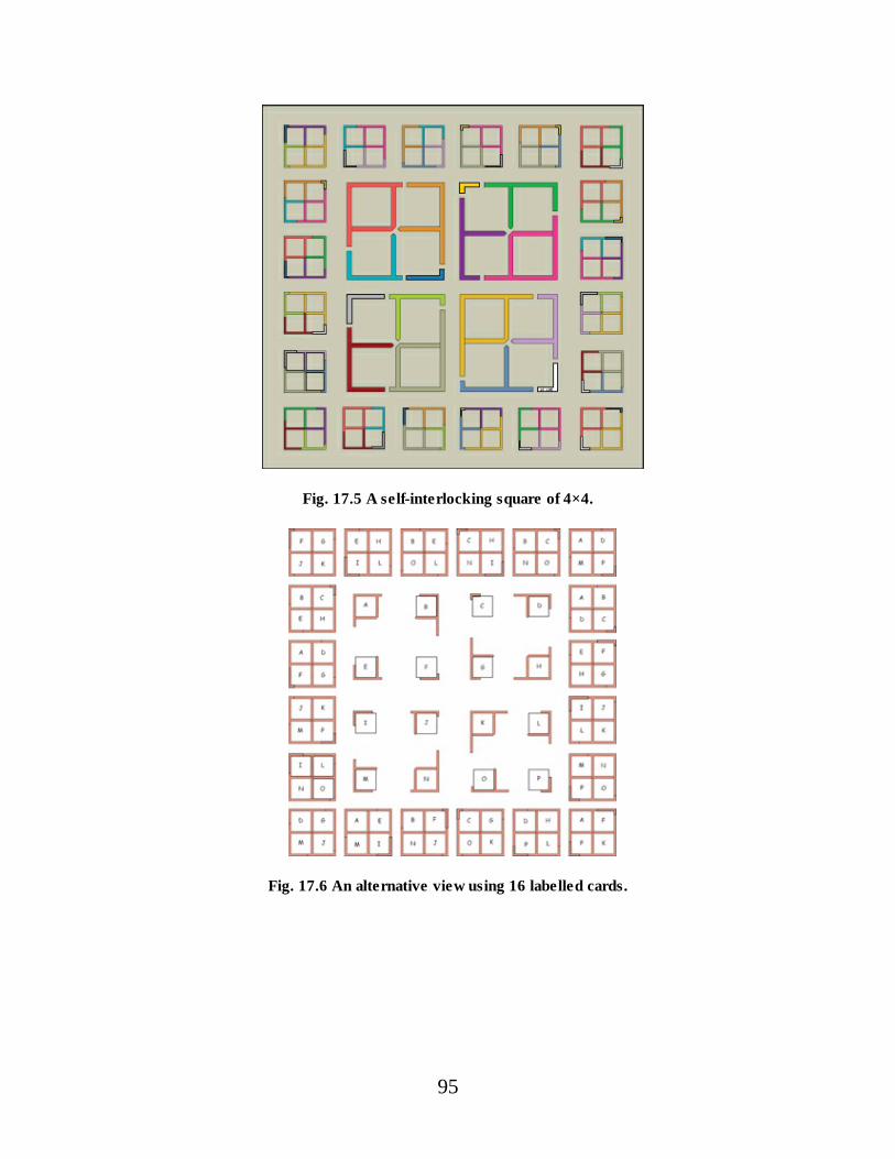
Fig. 17.5 A self-interlocking square of 4×4.

Fig. 17.6 An alternative view using 16 labelled cards.

95

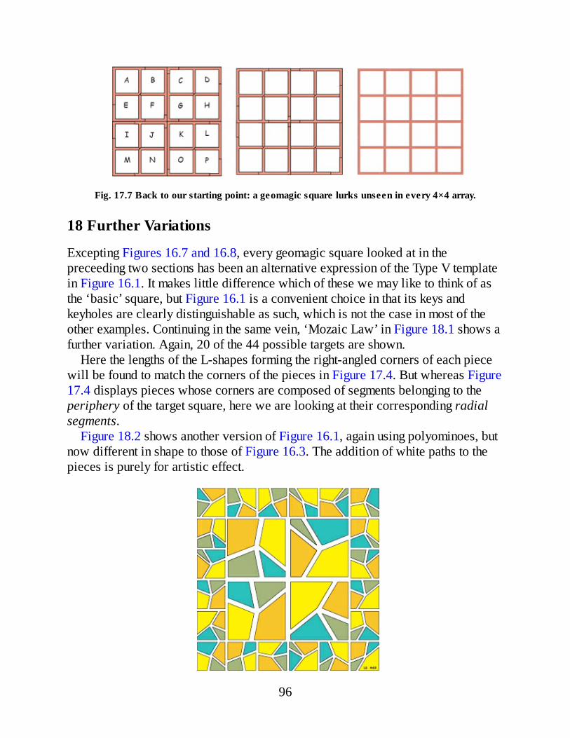
Fig. 17.7 Back to our starting point: a geomagic square lurks unseen in every 4×4 array.

18 Further Variations

Excepting Figures 16.7 and 16.8, every geomagic square looked at in thepreceeding two sections has been an alternative expression of the Type V templatein Figure 16.1. It makes little difference which of these we may like to think of asthe ‘basic’ square, but Figure 16.1 is a convenient choice in that its keys andkeyholes are clearly distinguishable as such, which is not the case in most of theother examples. Continuing in the same vein, ‘Mozaic Law’ in Figure 18.1 shows afurther variation. Again, 20 of the 44 possible targets are shown.

Here the lengths of the L-shapes forming the right-angled corners of each piecewill be found to match the corners of the pieces in Figure 17.4. But whereas Figure17.4 displays pieces whose corners are composed of segments belonging to theperiphery of the target square, here we are looking at their corresponding radialsegments.

Figure 18.2 shows another version of Figure 16.1, again using polyominoes, butnow different in shape to those of Figure 16.3. The addition of white paths to thepieces is purely for artistic effect.

96

Fig. 18.1 ‘Mozaic Law’ or the rules governing quasi-paving.

Figure 18.3 explains the design of piece shapes in Figures 16.3 and 18.2. Recallthat in both cases, the substrate from which we start is simply an identical square-shaped piece in every cell. Those used in Figure 16.3 are of size 4×4, those inFigure 18.2 of size 3×3; both of which are shown shaded in Figure 18.3. Keys andkeyholes are then appended to or excised from each piece as dictated by the TypeV template in Figure 16.1. The key corresponding to both p and q is a monominothat is appended to the square in two distinct positions. Similarly, the keycorresponding to both r and s is a domino, again affixed in two distinct positions.The 4 pieces shown in Figure 18.3 are those corresponding to p + q, – p – q, r + sand – r – s in the Type V template.

Fig. 18.2 Yet another interpretation of the Type V square in Figure 16.1.

Fig. 18.3 Piece shape design in Figure 16.3 (left) and Figure 18.2 (right).

97

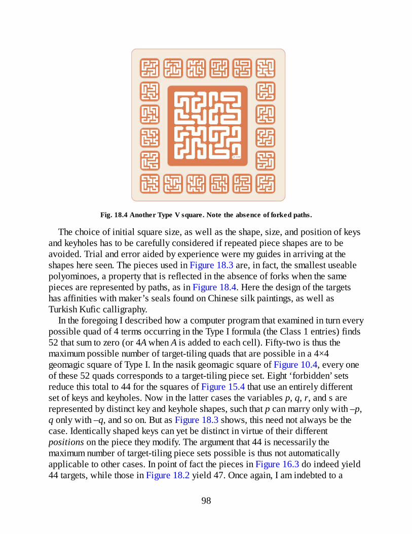
Fig. 18.4 Another Type V square. Note the absence of forked paths.

The choice of initial square size, as well as the shape, size, and position of keysand keyholes has to be carefully considered if repeated piece shapes are to beavoided. Trial and error aided by experience were my guides in arriving at theshapes here seen. The pieces used in Figure 18.3 are, in fact, the smallest useablepolyominoes, a property that is reflected in the absence of forks when the samepieces are represented by paths, as in Figure 18.4. Here the design of the targetshas affinities with maker’s seals found on Chinese silk paintings, as well asTurkish Kufic calligraphy.

In the foregoing I described how a computer program that examined in turn everypossible quad of 4 terms occurring in the Type I formula (the Class 1 entries) finds52 that sum to zero (or 4A when A is added to each cell). Fifty-two is thus themaximum possible number of target-tiling quads that are possible in a 4×4geomagic square of Type I. In the nasik geomagic square of Figure 10.4, every oneof these 52 quads corresponds to a target-tiling piece set. Eight ‘forbidden’ setsreduce this total to 44 for the squares of Figure 15.4 that use an entirely differentset of keys and keyholes. Now in the latter cases the variables p, q, r, and s arerepresented by distinct key and keyhole shapes, such that p can marry only with –p,q only with –q, and so on. But as Figure 18.3 shows, this need not always be thecase. Identically shaped keys can yet be distinct in virtue of their differentpositions on the piece they modify. The argument that 44 is necessarily themaximum number of target-tiling piece sets possible is thus not automaticallyapplicable to other cases. In point of fact the pieces in Figure 16.3 do indeed yield44 targets, while those in Figure 18.2 yield 47. Once again, I am indebted to a

98

computer program of Pat Hamlyn’s for ascertaining these results.Forty-seven targets can be formed with the pieces in Figure 18.2, but only 20 of

them are shown in the Figure. The explanation is artistic: 20 targets fit nicelyaround the central square; 47 would not. Only one more however will make 48,which is exactly the right number to complete a double border, a goal that isrealized in Figure 18.5, which is a geomagic square arrived at throughexperimenting with piece shapes derived from a different template.

The self-interlocking squares seen above have all been of Type V. Figure 18.5 isof Type VI, based on the template in Figure 18.6. Letters added to the pieces makeit easy to identify the composition of each target. Forty-four of the 48 targetscorrespond to the same quads of zero-totalling algebraic terms found in previoussquares. For example, the 4 pieces in the top row are a, b, c, and d.

The sum of their areas is thus (A + p + q) + (A -p + q) + (A + p – q) + (A – p –q) = 4A, the target area; see Figure 18.6. The 4 extra or abberent targets (over andabove the usual 44) occupy the outer corners of the border: defm. fgmp, ehmp, andacik. The area of the first is thus (A – p – q) + (A – q –r) + (A – q + r) + (A + r + s)= 4A –p – 3q + r + s. The key/keyhole sizes in Figure 18.5 are however the sameas in Figure 18.3 in which p = q = 1 and r = s 2, so that (– p – 3q + r + s) = 0, asrequired.

In the section to follow we shall take a closer look at the special topic of normalsquares, but for now I conclude this discussion of 4×4 geomagics with analternative rendering of the previous example. Figure 18.7 shows the same 16pieces together with their 48 targets, but here drawn together into a single seamlesssquare ‘carpet.’ Astrological signs, appropriate in view of their magicalconnotations, have replaced letters. I like to think that such a carpet would indeedfly, given only a carpet maker with the skill to weave it. In any case, many hourswent into the creation of this design. Perhaps those who can decipher theheiroglyphics will be able to discern here my personal offering to the god of magicsquares.

99

Fig. 18.5 A Type VI yielding 48 targets, enough for a double border.

Fig. 18.6 A Type VI template.

Fig. 18.7 A magic carpet that would really fly?

100

5 Due to author. The formula can be shown to be mininal in the sence of generalizing all 4×4 magic squaresmore economically than any other.

6 “Magic Formulae“ can be found as Appendix II.7 This formula is of special interest in bringing to light an archetypal 4×4 magic square, hetw =x = y = z = l,

with k = 0. Now interpret entries as 4-vectors; e.g., the bottom right hand entry becomes the vector [1,1,–1,–1].The result is a canonical 4×4 nasik square whose entries are the 16 vertices ofa2×2×2×2 tesseract centered onthe origin of 4-space!

101

Part III

Special CategoriesAn act of magic consists in doing what others believe is impossible.

19 2×2 Squares

If this were a book on numerical magic squares then the fact that we started withsquares of size 3×3 would make sense because they are the smallest possible. Fora 2×2 numagic square to be magic its four numbers must all be the same, as amoment’s reflection will show. But what about 2-D geometric magic squares; canan example be produced? I was so inured to the notion of 3×3 squares as smallestthat it was some time before this question so much as ocurred to mind. When it did,however, I found myself confronting a problem that, for all its seeming simplicity,would resist every attempt at solution, even following some years of thought.Indeed, to this day, the question of whether or not there exists such a square usingconnected pieces remains unanswered. Moreover, it wasn’t until quite recently -during the writing of this book -that Frank Tinkelenberg, a Dutch softwaredeveloper in Leyden, came up with the very first specimen. It is one among fourexamples that employ disconnected pieces.

Before coming to Tinkelenberg’s solution, we may note that 2×2 ‘semi-magic’ or‘orthomagic’ squares using connected pieces do indeed exist. These are squaresthat are magic on rows and columns only. Figure 19.1 shows an example usingpolyominoes of two sizes, 11 and 12.

Clearly a fully magic specimen would have to exhibit four pieces of equal size.Semi-magics with this latter property can be found. Figure 19.2 shows a secondsemi-magic square, the rows and columns of which remain magic whatever thewidth of rectangle R. Note that the areas of the two green pieces are both 24, whilethe areas of the remaining two pieces are 14 added to the area of R. Hence theareas of all 4 pieces will be equal when the area of R is 10, which is to say, whenits width is 5/3. However, this brings us no nearer to our goal of a fully magicspecimen.

More impressive is an almost-magic 2×2 square due to Michael Reid that heproduced (without quite realizing it) in response to a question I posted on anInternet forum devoted to polyforms: “Can a set of four distinct planar forms befound such that any two of them will tile the same region?” Reid’s outlandish targetshape and complicated 12-polyhex pieces seen in Figure 19.3 are a tribute to hismastery in the field of polyforms.

102

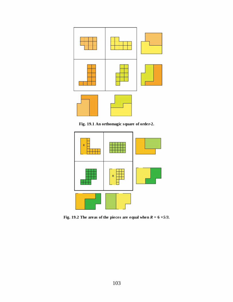
Fig. 19.1 An orthomagic square of order-2.

Fig. 19.2 The areas of the pieces are equal when R = 6 ×5/3.

103

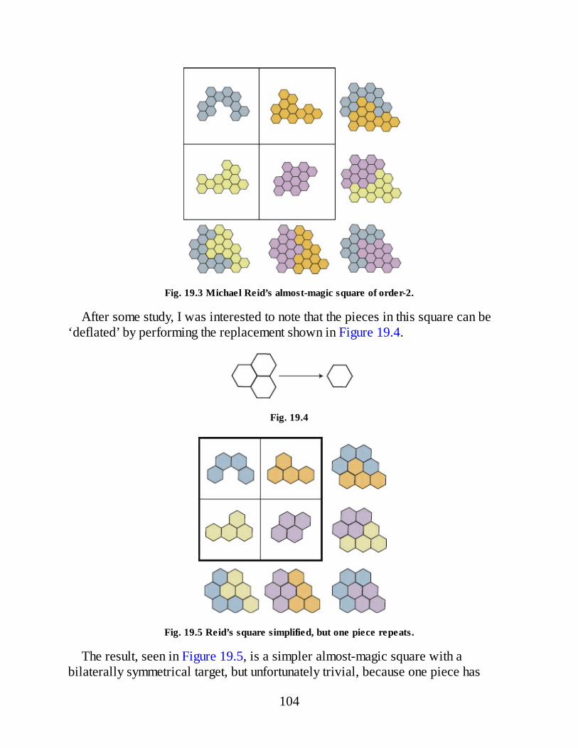
Fig. 19.3 Michael Reid’s almost-magic square of order-2.

After some study, I was interested to note that the pieces in this square can be‘deflated’ by performing the replacement shown in Figure 19.4.

Fig. 19.4

Fig. 19.5 Reid’s square simplified, but one piece repeats.

The result, seen in Figure 19.5, is a simpler almost-magic square with abilaterally symmetrical target, but unfortunately trivial, because one piece has

104

become the reflection of another. On the other hand, regarded as a set of threedistinct pieces, any two of which will tile the target, the same 4 polyhexes can beused to construct a peculiarly simple geomagic triangle, as demonstrated in Figure19.6. Two similar magic triangles can be constructed using three of Reid’s originalpieces.

Yet a further example of Reid’s inventive mind is his discovery of a non-trivial2×2 geomagic square using three-dimensional pieces. The idea can be pictured asfollows. Imagine four identical hollow hemispheres each pierced by a smallcircular hole in a different position. These are the four distinct pieces to be used inthe geomagic square. Now take any two hemispheres from this set of four. They canbe brought together and rotated with respect to each other so as to form the target,which is a hollow sphere having two holes separated by a certain fixed distance.That is all. It doesn’t matter which pair of hemispheres we begin with because asuitable rotation will always be able to adjust the hole-to-hole distance to thatrequired, whereas the lack of any reference point on the spherical surface makes itimpossible to speak meaningfully about the ‘position’ of any such pair. (This is oneof those ideas that is so simple that it has to be thought through three times before itcan be understood). There are some limits to the minimum and maximum possibledistances between the two holes, both of which are functions of the angles betweenthe radii to the centre of the holes and the plane of the ‘equator’ joining thehemispheres.

It is interesting to note that, as with any fully magic 2×2 geomagic square, thepieces used in Reid’s 3-D solution can be rearranged to yield three distinct 2×2squares, all of them nasik, as shown in Figure 19.7.

Fig. 19.6 A geomagic triangle.

105

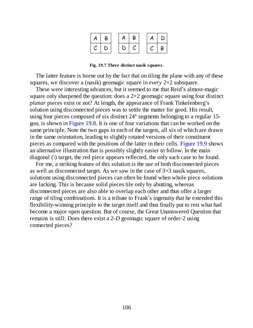
Fig. 19.7 Three distinct nasik squares.

The latter feature is borne out by the fact that on tiling the plane with any of thesesquares, we discover a (nasik) geomagic square in every 2×2 subsquare.

These were interesting advances, but it seemed to me that Reid’s almost-magicsquare only sharpened the question: does a 2×2 geomagic square using four distinctplanar pieces exist or not? At length, the appearance of Frank Tinkelenberg’ssolution using disconnected pieces was to settle the matter for good. His result,using four pieces composed of six distinct 24º segments belonging to a regular 15-gon, is shown in Figure 19.8. It is one of four variations that can be worked on thesame principle. Note the two gaps in each of the targets, all six of which are drawnin the same orientation, leading to slightly rotated versions of their constituentpieces as compared with the positions of the latter in their cells. Figure 19.9 showsan alternative illustration that is possibly slightly easier to follow. In the maindiagonal (\) target, the red piece appears reflected, the only such case to be found.

For me, a striking feature of this solution is the use of both disconnected piecesas well as disconnected target. As we saw in the case of 3×3 nasik squares,solutions using disconnected pieces can often be found when whole piece solutionsare lacking. This is because solid pieces tile only by abutting, whereasdisconnected pieces are also able to overlap each other and thus offer a largerrange of tiling combinations. It is a tribute to Frank’s ingenuity that he extended thisflexibility-winning principle to the target itself and thus finally put to rest what hadbecome a major open question. But of course, the Great Unanswered Question thatremains is still: Does there exist a 2-D geomagic square of order-2 usingconnected pieces?

106

Fig. 19.8 Frank Tinkelenberg’s 2×2 square.

107

Fig. 19.9 An alternative version of Tinkelenberg’s square.

20 Picture-Preserving Geomagics

A remarkable new development that took me completely by surprise was thediscovery of what I now call ‘picture-preserving’ geomagic squares, a wonderfulidea due to Robert Fathauer, presently living in Arizona. Robert, who introducedhimself to me following a talk I gave on geometric magic squares at the 2006Gathering for Gardner 7 conference in Atlanta, Georgia, runs a firm specializing inthe design and manufacture of educational aids used in teaching mathematics. Assuch, geomagic squares held for him a peculiar interest, his idea being to producephysical models using real pieces that might be used to illustrate elementarytheorems or other aspects of number theory. Initially I was a little unclear aboutthese proposals until he sent me the square shown in Figure 20.1. It is a modifiedversion of Figure 6.1 on page 12, which I had sent him previously, being one of the1,411 normal geomagic squares tiling a 3×5 rectangular target. The square can beseen again in Figure 20.3 (left).

Fig. 20.1 Robert Fathauer’s picture-preserving geomagic square.

At first sight it may seem that there are two pieces occupying each cell in Figure20.1. This, however, is not really the case, the intention being rather to show whatis printed on the front and back faces of the single piece occupying each cell. The

108

two shapes in each cell are thus reflections of each other, although in several casesthe flipped twin has been rotated so as to bring the numbers printed on both sidesright side up. Simply flipping a piece about a vertical or horizontal axis, withoutrotation, will often reveal numbers that are printed either upside down orsideways. To avoid this, the orientation of each piece shown in the cells has beenchosen so as to show the digits right side up, which is the same as that in the targetsin which they appear.

Two distinct shades of blue distinguish fronts from backs, making it easier to seehow targets are composed of flipped and/or unflipped pieces. In a physicalrealization using real pieces this would be unnecessary. Using the same tint on bothsides would then make for targets of uniform color. As in the square on which it isbased (i.e. Figure 20.3), the target is again a rectangle, but now bearing thenumbers from 1 to 15 in serial order. The idea was to use this as a didactic devicein combination with a worksheet discussing how to sum the first n natural numbers.It took me a few minutes to figure out the extraordinary implication of whatFathauer had achieved in his modified version of my square.

Every piece bears numbers, front and back, such that the target is not merely arectangle, but one in which these numbers appear in serial order from left to right.The individual numbered cells thus appear in exactly the same position in everytarget, and the same would be true whether or not these cells bore numbers or someother graphical device. In particular, that device might be a square fragmentbelonging to a given position within any 3×5 field or ‘picture.’ But in that case thepieces in the cells would themselves correspond to larger picture fragments thatassemble in the targets so as to reproduce the entire 3×5 field. Targets will then notonly share the same outline shape, their surface detail will also be identical, pointfor point, or if you will, pixel for pixel. Hence the appellation ‘picture-preserving’(or ‘pp’) for a geomagic square of this kind, although in the case of Fathauer’ssquare the ‘picture’ is less a tableau or view than it is an austere table of numbers.Figure 20.2 exploits the pp-property to better effect, the target here being the Fiveof Hearts playing card. To avoid overcrowding, the reverse sides of the pieces arenot shown in the cells, but can be inferred from the targets. For instance, from theleft-hand-column target can be seen that the square piece that is blank (seen in theleft-hand column centre cell) bears two half-hearts on its reverse side.

109

Fig. 20.2 A picture-preserving square.

What is the essential property that distinguishes picture-preserving geomagicsfrom others? It is that wherever any given piece occurs in different targets, italways occupies exactly the same position within each of them. For only thus willevery picture fragment always find itself in its appropriate place within theassembled picture. Yet, since the flip side of a reflected piece may bear distinctmarkings, in this respect a reversed piece may be treated as a separate case. Thesepoints will becime clearer on examining the differences between Fathauer’s squareand the square from which it was derived, shown in Figure 20.3. For example, thegrey octomino in the top left hand cell of the latter does indeed occupy the sameposition in all three targets in which it appears. But the blue hexomino in the topright hand cell occupies distinct positions in different targets, a feature that willdisrupt picture preservation. A reflected version of this same piece occurs justonce, in the top row target only, which is unproblematical, because the imagedepicted on its back side can be adjusted to suit that distinct region of the picture itoccupies. Observe also that the domino in the bottom right hand cell may or maynot be said to appear in three different targets, depending upon whether one ormore of these is regarded as flipped or not. In any case, it was Fathauer’s insight tosee that with a few judicious adjustments to the orientation of certain targets, theseproblems could all be overcome, as witnessed in his modified version of the samegeomagic square seen in Figure 20.3 (right).

110

Here the previously troublesome hexomino now occupies the same positionwithin two targets, as does the domino, whose seeming third appearance in thediagonal target can now be interpreted as a reflected domino, occurring but once.Similar comments apply to the tetromino in the bottom left-hand cell, which, likethe monomino, domino, and triomino, is another case of a piece whose flipped andunflipped forms are congruent. Figure 20.3 (right) is thus suitable for use as a pp-geomagic square, as indeed it has been in providing the basis for Figure 20.1.

Fig. 20.3 Converting an ordinary square into a picture-preserver.

Having grasped the principle underlying Fathauer’s square, it was natural tostart re-examining existing geomagics in the hope of discovering still more picture-preservers. Was it significant that his square is derived from a specimen usingpolyominoes of consecutive sizes? Figure 20.2, an early find, which is also amongthe 1,411 geomagics using consecutively sized polyominoes, suggested it might be,although subsequent examples lent no support to this idea.

The picture-preserving property is perhaps easier to follow in Figure 20.4, inwhich the ‘picture’ is no more than a yellow circle centred on a green square. Seento right and below are reflected versions of the eight targets (flipped about avertical axis), revealing the jumbled patterns incidentally created on their reversedsides. This specimen is based on Figure 20.5, an earlier discovered (symmetric)geometric square. Interested readers may like to examine the small, yet subtle,changes to the targets that converted this initial find into a picture-preserver. Notethat use of a circle as a target picture makes for a special case that forms anexception to the general rule enunciated previously. That the same piece mustoccupy the same position within different targets is no longer necessarily true,since the symmetry of the circle means that it can be repeatedly rotated through 90º

111

without any change to the ‘picture.’

Fig. 20.4 The ‘picture’ is a yellow circle on a green square.

The square target in Figure 20.5 is of size 6×6. An obvious idea suggested bythis was to replace the circle motif with a picture showing a 6×6 numagic squareas target. Piece edges would then correspond with grid lines on the 6×6 array,much as in Fathauer’s numbered 3×5 target. An experiment showed this to be quitefeasible, although the swarms of numbered cells involved make for a pictoriallyinelegant result. In view of this, a better idea seemed to be a target using a visuallysimpler square such as the Lo shu. Grid lines in the square will then no longercorrespond with piece edges, and in fact some numerals end up becoming bisected,an outcome that, in retrospect, seems less than satisfactory. Figure 20.6 shows theresulting square. Light and dark shading distinguish piece fronts from backs.

112

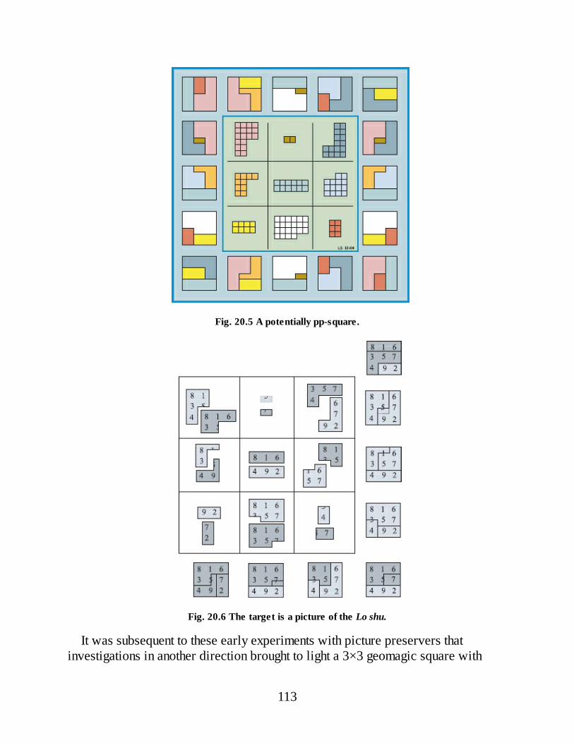
Fig. 20.5 A potentially pp-square.

Fig. 20.6 The target is a picture of the Lo shu.

It was subsequent to these early experiments with picture preservers thatinvestigations in another direction brought to light a 3×3 geomagic square with

113

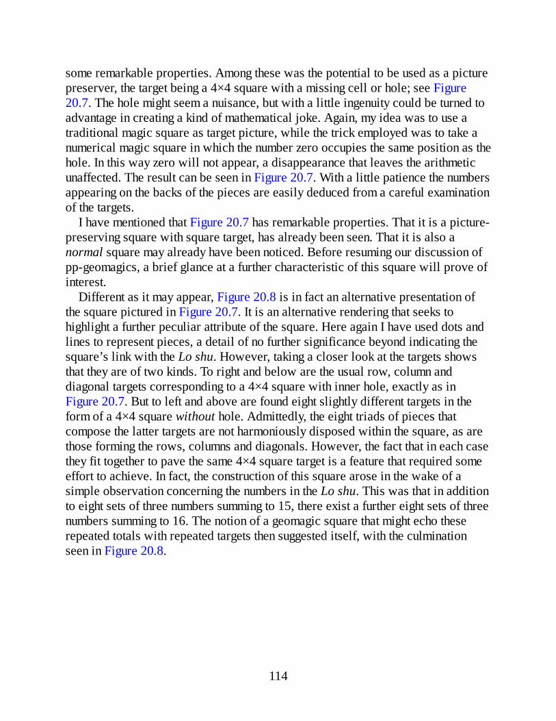
some remarkable properties. Among these was the potential to be used as a picturepreserver, the target being a 4×4 square with a missing cell or hole; see Figure20.7. The hole might seem a nuisance, but with a little ingenuity could be turned toadvantage in creating a kind of mathematical joke. Again, my idea was to use atraditional magic square as target picture, while the trick employed was to take anumerical magic square in which the number zero occupies the same position as thehole. In this way zero will not appear, a disappearance that leaves the arithmeticunaffected. The result can be seen in Figure 20.7. With a little patience the numbersappearing on the backs of the pieces are easily deduced from a careful examinationof the targets.

I have mentioned that Figure 20.7 has remarkable properties. That it is a picture-preserving square with square target, has already been seen. That it is also anormal square may already have been noticed. Before resuming our discussion ofpp-geomagics, a brief glance at a further characteristic of this square will prove ofinterest.

Different as it may appear, Figure 20.8 is in fact an alternative presentation ofthe square pictured in Figure 20.7. It is an alternative rendering that seeks tohighlight a further peculiar attribute of the square. Here again I have used dots andlines to represent pieces, a detail of no further significance beyond indicating thesquare’s link with the Lo shu. However, taking a closer look at the targets showsthat they are of two kinds. To right and below are the usual row, column anddiagonal targets corresponding to a 4×4 square with inner hole, exactly as inFigure 20.7. But to left and above are found eight slightly different targets in theform of a 4×4 square without hole. Admittedly, the eight triads of pieces thatcompose the latter targets are not harmoniously disposed within the square, as arethose forming the rows, columns and diagonals. However, the fact that in each casethey fit together to pave the same 4×4 square target is a feature that required someeffort to achieve. In fact, the construction of this square arose in the wake of asimple observation concerning the numbers in the Lo shu. This was that in additionto eight sets of three numbers summing to 15, there exist a further eight sets of threenumbers summing to 16. The notion of a geomagic square that might echo theserepeated totals with repeated targets then suggested itself, with the culminationseen in Figure 20.8.

114

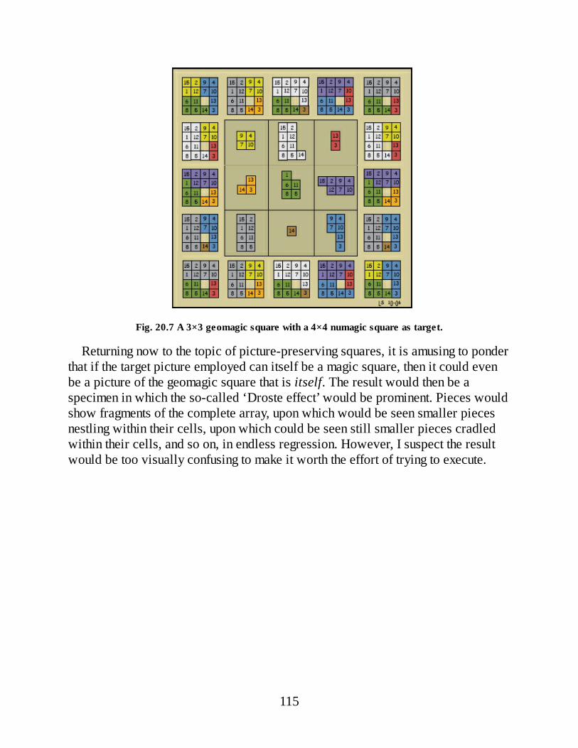
Fig. 20.7 A 3×3 geomagic square with a 4×4 numagic square as target.

Returning now to the topic of picture-preserving squares, it is amusing to ponderthat if the target picture employed can itself be a magic square, then it could evenbe a picture of the geomagic square that is itself. The result would then be aspecimen in which the so-called ‘Droste effect’ would be prominent. Pieces wouldshow fragments of the complete array, upon which would be seen smaller piecesnestling within their cells, upon which could be seen still smaller pieces cradledwithin their cells, and so on, in endless regression. However, I suspect the resultwould be too visually confusing to make it worth the effort of trying to execute.

115

Fig. 20.8 Different as it seems, this is the same square as in Figure 20.7.

Fig. 20.9 A chequered target reveals the picture-preserving property of Figure 9.7.

The pp-geomagics looked at thus far have all been of size 3×3. It is easy to seethan no 2×2 examples will be found. Given that each piece would need to occupyan identical position in at least two different targets, the shape of the remainingtarget area, which is to say, the shape of the second piece, would then have to be

116

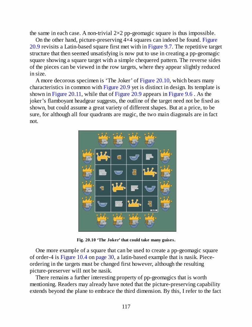
the same in each case. A non-trivial 2×2 pp-geomagic square is thus impossible.On the other hand, picture-preserving 4×4 squares can indeed be found. Figure

20.9 revisits a Latin-based square first met with in Figure 9.7. The repetitive targetstructure that then seemed unsatisfying is now put to use in creating a pp-geomagicsquare showing a square target with a simple chequered pattern. The reverse sidesof the pieces can be viewed in the row targets, where they appear slightly reducedin size.

A more decorous specimen is ‘The Joker’ of Figure 20.10, which bears manycharacteristics in common with Figure 20.9 yet is distinct in design. Its template isshown in Figure 20.11, while that of Figure 20.9 appears in Figure 9.6 . As thejoker’s flamboyant headgear suggests, the outline of the target need not be fixed asshown, but could assume a great variety of different shapes. But at a price, to besure, for although all four quadrants are magic, the two main diagonals are in factnot.

Fig. 20.10 ‘The Joker’ that could take many guises.

One more example of a square that can be used to create a pp-geomagic squareof order-4 is Figure 10.4 on page 30, a latin-based example that is nasik. Piece-ordering in the targets must be changed first however, although the resultingpicture-preserver will not be nasik.

There remains a further interesting property of pp-geomagics that is worthmentioning. Readers may already have noted that the picture-preserving capabilityextends beyond the plane to embrace the third dimension. By this, I refer to the fact

117

that the targets in a pp-square can include pictures carved in relief, so long as weare prepared to ignore that part of the target structure on its reverse side,protruding backwards behind the plane that is its floor. To grasp this, imagine thepicture in Figure 20.4 is not a circle but a solid cone, seen from above, the pointedend. The various pieces thus bear complicated dissections of this cone, which hasbeen sliced by planes that are perpendicular to its base. On the reverse sides ofpieces are similar dissections that extend away from the viewer rather than toward.In the targets we view the reconstructed solid cones, although behind them is anunholy chaos, equally three-dimensional, corresponding to the jumbled patternsseen in the reversed targets of the same figure. Granted that this feature would notseem to be of any particular ‘use,’ I find it intriguing. My own belief is that the lastword on pp-geomagics has yet to be said.

Fig. 20.11 The Joker’s template.

118

Fig. 20.12 Is this a trivial square, or not?

A final point of interest is to see how the introduction of the pp-geomagic squarebrings with it the need for a clarification in our definition of ‘trivial’. Figure 20.12,a supposedly trival square, illustrates the point, its square target, again a picture ofthe Lo shu, being formed from pieces of repeated shape, which are neverthelessdistinct in virtue of their unique marking. So, we may ask, is Figure 20.12 reallytrivial or not? The answer is of little import, of course, but the point is worthbearing in mind.

I can hardly conclude this section on picture-preservers without showing anunusual find of order-3 that lent itself to a playful elaboration. There exists aspecial kind of picture-preserver that requires no markings on the back sides of itspieces because every target can be assembled without reversing any piece. Such asquare is seen in ‘The Archaeologist’s Nightmare’ of Figure 20.13, where theimplied concavity of the plate would make flipped pieces inappropriate. Givensuitable marking on the hidden sides of the present pieces, the potter’s trademarkcould be made to appear on the underside of each reassembled plate. Although notshown, the three shards on each diagonal can also be glued together to form theplate.

It may interest readers to learn that I submitted this picture to the British Journalof Archaeology, confident of its being enthusiastically received as a humorousfiller item for the journal. However, I was wrong. They were not amused.

119

Fig. 20.13 ‘The Archaeologist’s Nightmare.’

21 3-Dimensional Geomagics

The allusion to solid targets in the previous section brings us nicely to the topic of3-dimensional geomagic squares. As indicated at the outset of this essay,geomagics may use pieces of any dimension, although for practical reasons 2-Dtypes are bound to exert the greater appeal, since they are both easier to produce,as well as simple to present on the page and to think about and discuss. 3-Dsquares are not merely less ubiquitous, and thus more difficult to track down, theydo not lend themselves to presentation on paper, being best appreciated in the formof solid objects that can be picked up and handled. And of course, the manufactureof such material objects is a demanding enough hobby in its own right, withoutadding the exigencies of writing a computer program for discovering thegeometrical forms that are to be constructed. Indeed, bearing in mind the sheerwork involved in exploring planar types, in retrospect it seems surprising I everstarted in pursuit of the far more demanding 3-D specimens. But the truth is that Iwas spurred on by the attractions of one particular solid target that caught my fancy.

If the aim was to construct a geomagic square using solid pieces that fit togetherso as to complete a solid target then a square of order-3 was the obvious case toconsider. Being unable to think up any alternative approach, a computer programperforming a brute-force search offered the only possibility of discovering a

120

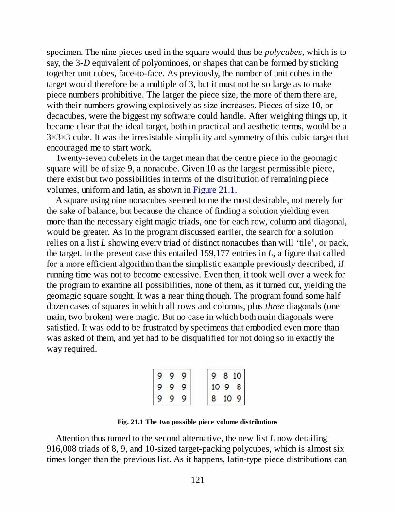
specimen. The nine pieces used in the square would thus be polycubes, which is tosay, the 3-D equivalent of polyominoes, or shapes that can be formed by stickingtogether unit cubes, face-to-face. As previously, the number of unit cubes in thetarget would therefore be a multiple of 3, but it must not be so large as to makepiece numbers prohibitive. The larger the piece size, the more of them there are,with their numbers growing explosively as size increases. Pieces of size 10, ordecacubes, were the biggest my software could handle. After weighing things up, itbecame clear that the ideal target, both in practical and aesthetic terms, would be a3×3×3 cube. It was the irresistable simplicity and symmetry of this cubic target thatencouraged me to start work.

Twenty-seven cubelets in the target mean that the centre piece in the geomagicsquare will be of size 9, a nonacube. Given 10 as the largest permissible piece,there exist but two possibilities in terms of the distribution of remaining piecevolumes, uniform and latin, as shown in Figure 21.1.

A square using nine nonacubes seemed to me the most desirable, not merely forthe sake of balance, but because the chance of finding a solution yielding evenmore than the necessary eight magic triads, one for each row, column and diagonal,would be greater. As in the program discussed earlier, the search for a solutionrelies on a list L showing every triad of distinct nonacubes than will ‘tile’, or pack,the target. In the present case this entailed 159,177 entries in L, a figure that calledfor a more efficient algorithm than the simplistic example previously described, ifrunning time was not to become excessive. Even then, it took well over a week forthe program to examine all possibilities, none of them, as it turned out, yielding thegeomagic square sought. It was a near thing though. The program found some halfdozen cases of squares in which all rows and columns, plus three diagonals (onemain, two broken) were magic. But no case in which both main diagonals weresatisfied. It was odd to be frustrated by specimens that embodied even more thanwas asked of them, and yet had to be disqualified for not doing so in exactly theway required.

Fig. 21.1 The two possible piece volume distributions

Attention thus turned to the second alternative, the new list L now detailing916,008 triads of 8, 9, and 10-sized target-packing polycubes, which is almost sixtimes longer than the previous list. As it happens, latin-type piece distributions can

121

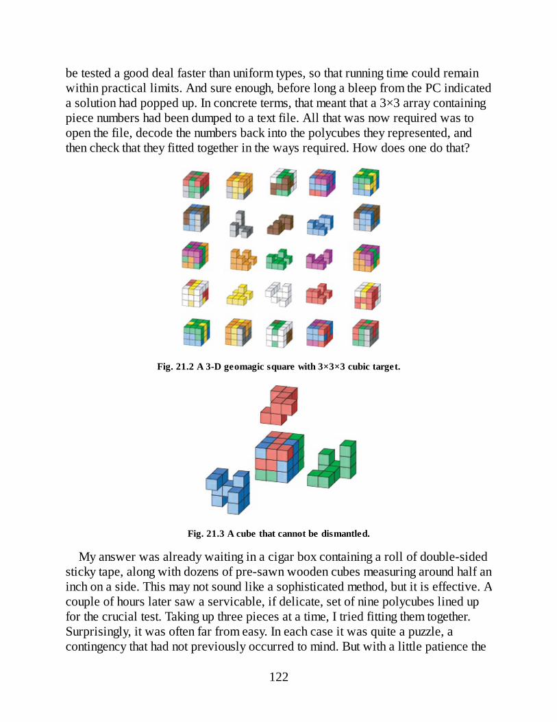
be tested a good deal faster than uniform types, so that running time could remainwithin practical limits. And sure enough, before long a bleep from the PC indicateda solution had popped up. In concrete terms, that meant that a 3×3 array containingpiece numbers had been dumped to a text file. All that was now required was toopen the file, decode the numbers back into the polycubes they represented, andthen check that they fitted together in the ways required. How does one do that?

Fig. 21.2 A 3-D geomagic square with 3×3×3 cubic target.

Fig. 21.3 A cube that cannot be dismantled.

My answer was already waiting in a cigar box containing a roll of double-sidedsticky tape, along with dozens of pre-sawn wooden cubes measuring around half aninch on a side. This may not sound like a sophisticated method, but it is effective. Acouple of hours later saw a servicable, if delicate, set of nine polycubes lined upfor the crucial test. Taking up three pieces at a time, I tried fitting them together.Surprisingly, it was often far from easy. In each case it was quite a puzzle, acontingency that had not previously occurred to mind. But with a little patience the

122

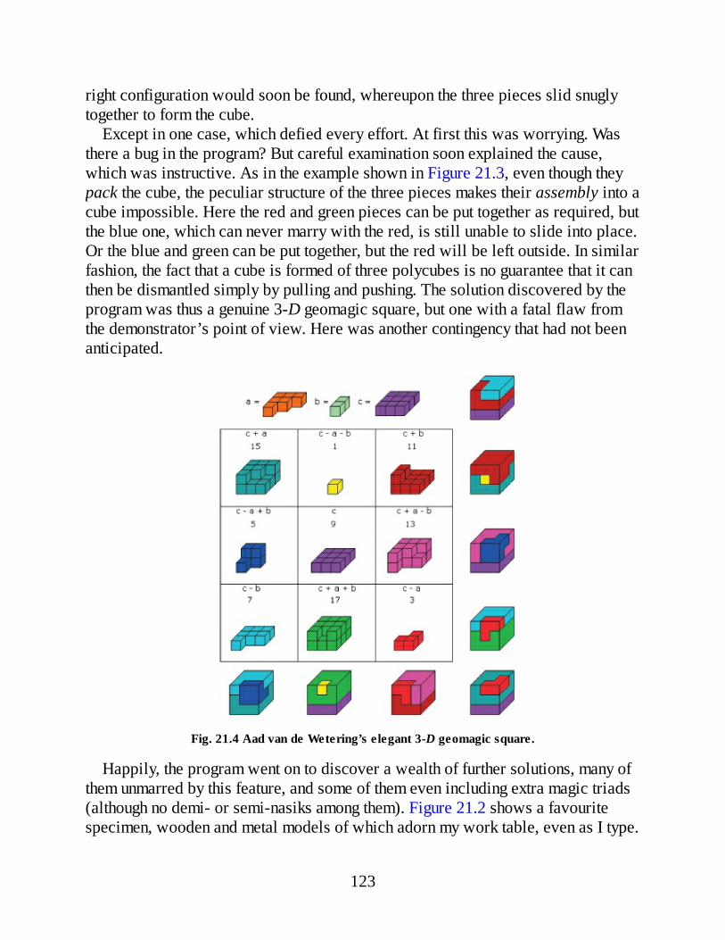
right configuration would soon be found, whereupon the three pieces slid snuglytogether to form the cube.

Except in one case, which defied every effort. At first this was worrying. Wasthere a bug in the program? But careful examination soon explained the cause,which was instructive. As in the example shown in Figure 21.3, even though theypack the cube, the peculiar structure of the three pieces makes their assembly into acube impossible. Here the red and green pieces can be put together as required, butthe blue one, which can never marry with the red, is still unable to slide into place.Or the blue and green can be put together, but the red will be left outside. In similarfashion, the fact that a cube is formed of three polycubes is no guarantee that it canthen be dismantled simply by pulling and pushing. The solution discovered by theprogram was thus a genuine 3-D geomagic square, but one with a fatal flaw fromthe demonstrator’s point of view. Here was another contingency that had not beenanticipated.

Fig. 21.4 Aad van de Wetering’s elegant 3-D geomagic square.

Happily, the program went on to discover a wealth of further solutions, many ofthem unmarred by this feature, and some of them even including extra magic triads(although no demi- or semi-nasiks among them). Figure 21.2 shows a favouritespecimen, wooden and metal models of which adorn my work table, even as I type.

123

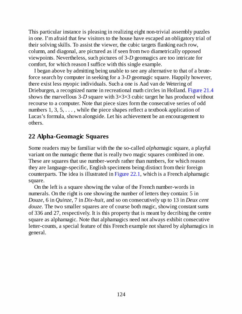
This particular instance is pleasing in realizing eight non-trivial assembly puzzlesin one. I’m afraid that few visitors to the house have escaped an obligatory trial oftheir solving skills. To assist the viewer, the cubic targets flanking each row,column, and diagonal, are pictured as if seen from two diametrically opposedviewpoints. Nevertheless, such pictures of 3-D geomagics are too intricate forcomfort, for which reason I suffice with this single example.

I began above by admitting being unable to see any alternative to that of a brute-force search by computer in seeking for a 3-D geomagic square. Happily however,there exist less myopic individuals. Such a one is Aad van de Wetering ofDrieburgen, a recognized name in recreational math circles in Holland. Figure 21.4shows the marvellous 3-D square with 3×3×3 cubic target he has produced withoutrecourse to a computer. Note that piece sizes form the consecutive series of oddnumbers 1, 3, 5, . . . , while the piece shapes reflect a textbook application ofLucas’s formula, shown alongside. Let his achievement be an encouragement toothers.

22 Alpha-Geomagic Squares

Some readers may be familiar with the the so-called alphamagic square, a playfulvariant on the numagic theme that is really two magic squares combined in one.These are squares that use number-words rather than numbers, for which reasonthey are language-specific, English specimens being distinct from their foreigncounterparts. The idea is illustrated in Figure 22.1, which is a French alphamagicsquare.

On the left is a square showing the value of the French number-words innumerals. On the right is one showing the number of letters they contain: 5 inDouze, 6 in Quinze, 7 in Dix-huit, and so on consecutively up to 13 in Deux centdouze. The two smaller squares are of course both magic, showing constant sumsof 336 and 27, respectively. It is this property that is meant by decribing the centresquare as alphamagic. Note that alphamagics need not always exhibit consecutiveletter-counts, a special feature of this French example not shared by alphamagics ingeneral.

124

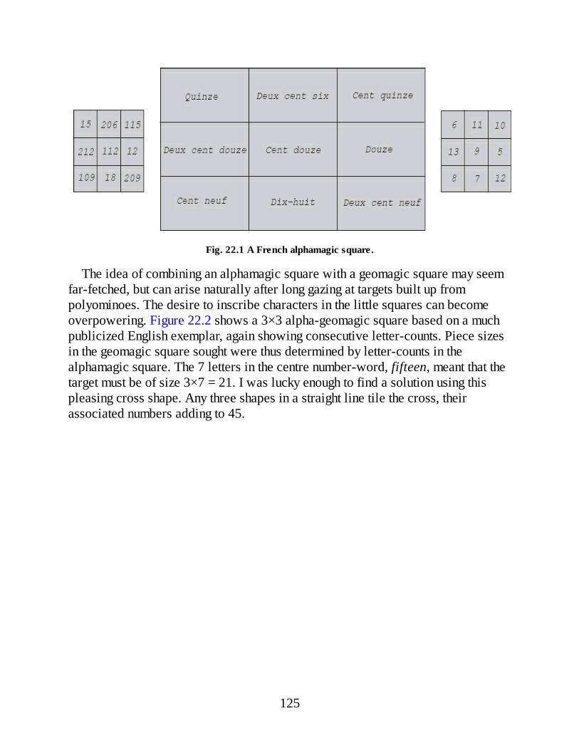
Fig. 22.1 A French alphamagic square.

The idea of combining an alphamagic square with a geomagic square may seemfar-fetched, but can arise naturally after long gazing at targets built up frompolyominoes. The desire to inscribe characters in the little squares can becomeoverpowering. Figure 22.2 shows a 3×3 alpha-geomagic square based on a muchpublicized English exemplar, again showing consecutive letter-counts. Piece sizesin the geomagic square sought were thus determined by letter-counts in thealphamagic square. The 7 letters in the centre number-word, fifteen, meant that thetarget must be of size 3×7 = 21. I was lucky enough to find a solution using thispleasing cross shape. Any three shapes in a straight line tile the cross, theirassociated numbers adding to 45.

125

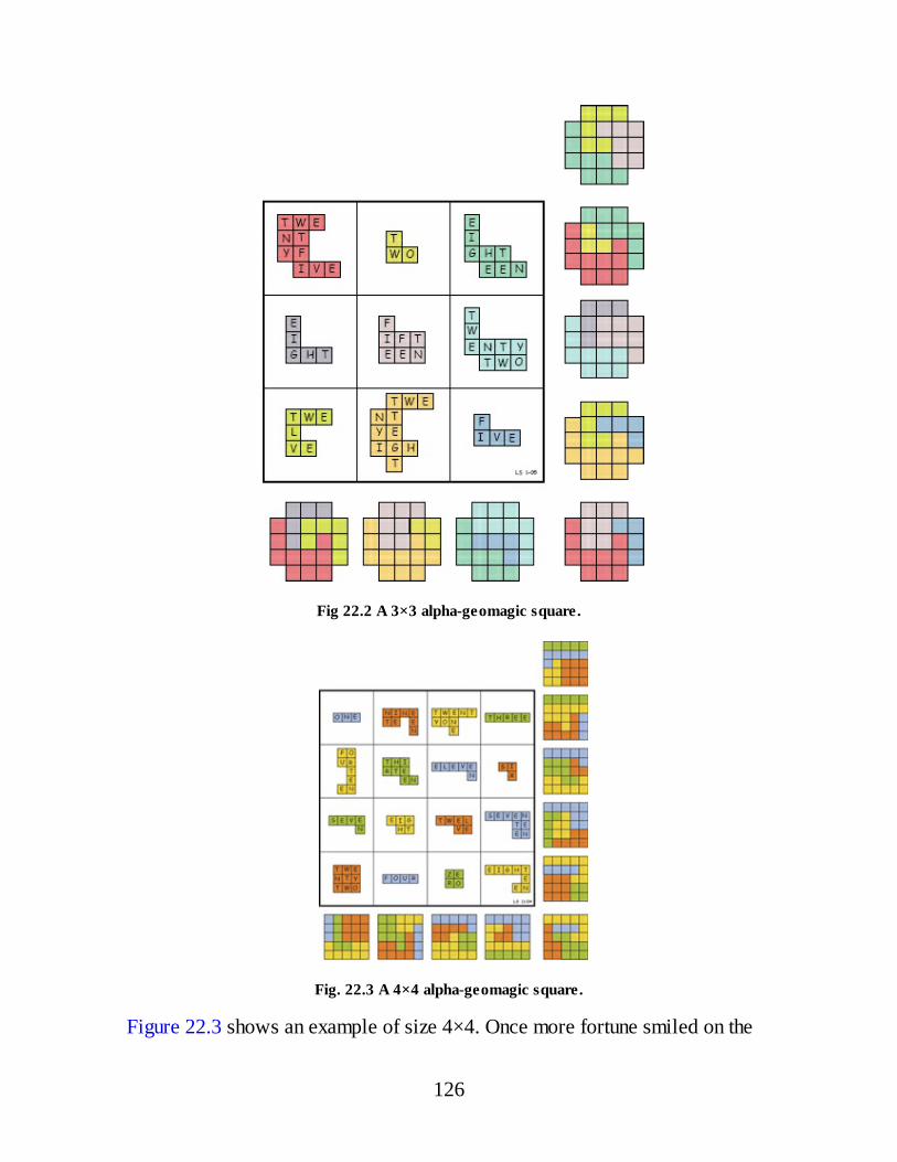
Fig 22.2 A 3×3 alpha-geomagic square.

Fig. 22.3 A 4×4 alpha-geomagic square.

Figure 22.3 shows an example of size 4×4. Once more fortune smiled on the

126

search for a 5×5 square target to accommodate a constant sum of 25 letterscontributed by the alphamagic square from which I started. Figure 22.4 shows analternative version of the same square.

Fig. 22.4 An alternative version of Figure 22.3.

23 Normal Squares of Order 4

In Part II we looked at various aspects of 4×4 squares but without paying anyspecial regard to their corresponding area squares. The latter are, of course,numerical magic squares in their own right, albeit ones in which the appearance ofrepeated values tends to discourage interest. An exceptional case that attractsspecial notice is thus that of the normal square in which the areas of the piecesform the arithmetic progression 1, 2, . . , 16.

How do we go about constructing a normal 2-D square? Since the area square isitself normal, it can only belong to one of Dudeney’s twelve Types. This suggestedthe idea of starting with a numerical magic square, the formula for which is thenconsulted in order to arrive at the key and keyhole areas that will be required toconstruct a 2-D version of the same square. An example will clarify this process.

Figure 23.1 shows ‘Melencolia I,’ a well-known engraving by the GermanRenaissance artist Albrecht Dürer. An allegorical composition, it has been the

127

subject of many interpretations. Among other symbols, it includes a 4×4 magicsquare using the numbers 1 to 16, with constant sum 34. A point of interest is thatthe date of the engraving, 1514, is given by the two centre numbers in the bottomrow. Here then is a normal numerical magic square that will serve to illlustrate thecreation of a normal 2-D square. Figure 23.2 shows a modern version of Durer’ssquare that is easier to read.

Fig. 23.1 ‘Melencolia’ by Albrecht Diirer.

Fig. 23.2 A clearer view of Diirer’s square.

A look at the distribution of the complementary pairs in Figure 23.2 shows thembalanced about the centre in a pattern corresponding to the Dudeney Type IIIdiagram. Figure 23.3 reproduces the generalization of Type III squares, seen earlierin Figure 13.2 on page 38. The values taken by the variables in the case of Durer’snumerical square are then easily derived:

128

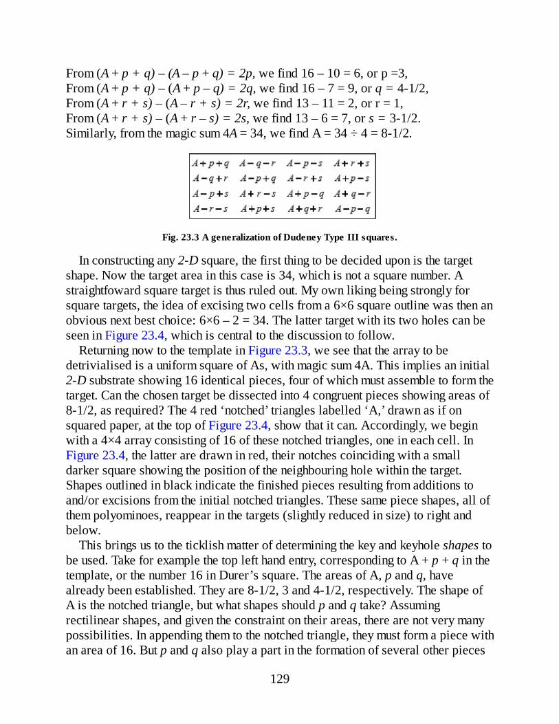
From (A + p + q) – (A – p + q) = 2p, we find 16 – 10 = 6, or p =3,From (A + p + q) – (A + p – q) = 2q, we find 16 – 7 = 9, or q = 4-1/2,From (A + r + s) – (A – r + s) = 2r, we find 13 – 11 = 2, or r = 1,From (A + r + s) – (A + r – s) = 2s, we find 13 – 6 = 7, or s = 3-1/2.Similarly, from the magic sum 4A = 34, we find A = 34 ÷ 4 = 8-1/2.

Fig. 23.3 A generalization of Dudeney Type III squares.

In constructing any 2-D square, the first thing to be decided upon is the targetshape. Now the target area in this case is 34, which is not a square number. Astraightfoward square target is thus ruled out. My own liking being strongly forsquare targets, the idea of excising two cells from a 6×6 square outline was then anobvious next best choice: 6×6 – 2 = 34. The latter target with its two holes can beseen in Figure 23.4, which is central to the discussion to follow.

Returning now to the template in Figure 23.3, we see that the array to bedetrivialised is a uniform square of As, with magic sum 4A. This implies an initial2-D substrate showing 16 identical pieces, four of which must assemble to form thetarget. Can the chosen target be dissected into 4 congruent pieces showing areas of8-1/2, as required? The 4 red ‘notched’ triangles labelled ‘A,’ drawn as if onsquared paper, at the top of Figure 23.4, show that it can. Accordingly, we beginwith a 4×4 array consisting of 16 of these notched triangles, one in each cell. InFigure 23.4, the latter are drawn in red, their notches coinciding with a smalldarker square showing the position of the neighbouring hole within the target.Shapes outlined in black indicate the finished pieces resulting from additions toand/or excisions from the initial notched triangles. These same piece shapes, all ofthem polyominoes, reappear in the targets (slightly reduced in size) to right andbelow.

This brings us to the ticklish matter of determining the key and keyhole shapes tobe used. Take for example the top left hand entry, corresponding to A + p + q in thetemplate, or the number 16 in Durer’s square. The areas of A, p and q, havealready been established. They are 8-1/2, 3 and 4-1/2, respectively. The shape ofA is the notched triangle, but what shapes should p and q take? Assumingrectilinear shapes, and given the constraint on their areas, there are not very manypossibilities. In appending them to the notched triangle, they must form a piece withan area of 16. But p and q also play a part in the formation of several other pieces

129

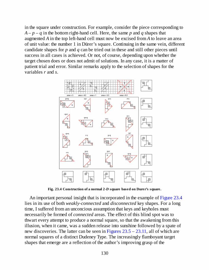
in the square under construction. For example, consider the piece corresponding toA – p – q in the bottom right-hand cell. Here, the same p and q shapes thataugmented A in the top left-hand cell must now be excised from A to leave an areaof unit value: the number 1 in Dürer’s square. Continuing in the same vein, differentcandidate shapes for p and q can be tried out in these and still other pieces untilsuccess in all cases is achieved. Or not, of course, depending upon whether thetarget chosen does or does not admit of solutions. In any case, it is a matter ofpatient trial and error. Similar remarks apply to the selection of shapes for thevariables r and s.

Fig. 23.4 Construction of a normal 2-D square based on Durer’s square.

An important personal insight that is incorporated in the example of Figure 23.4lies in its use of both weakly-connected and disconnected key shapes. For a longtime, I suffered from an unconcious assumption that keys and keyholes mustnecessarily be formed of connected areas. The effect of this blind spot was tothwart every attempt to produce a normal square, so that the awakening from thisillusion, when it came, was a sudden release into sunshine followed by a spate ofnew discoveries. The latter can be seen in Figures 23.5 – 23.11, all of which arenormal squares of a distinct Dudeney Type. The increasingly flamboyant targetshapes that emerge are a reflection of the author’s improving grasp of the

130

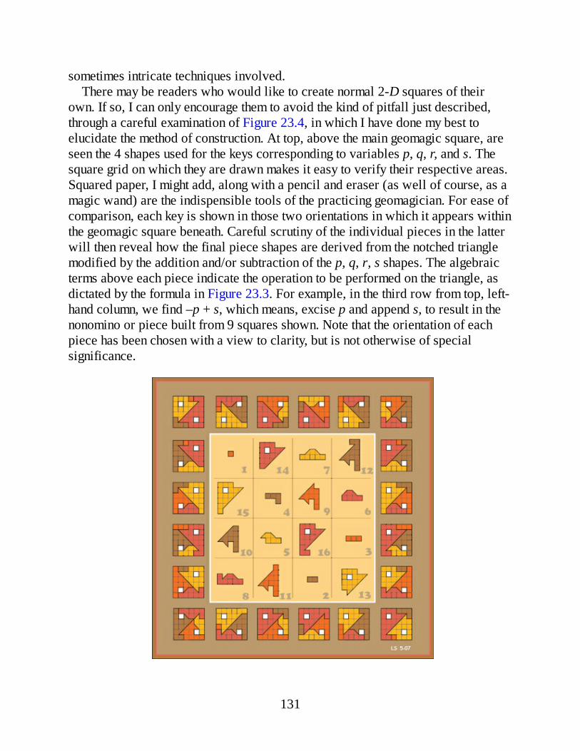
sometimes intricate techniques involved.There may be readers who would like to create normal 2-D squares of their

own. If so, I can only encourage them to avoid the kind of pitfall just described,through a careful examination of Figure 23.4, in which I have done my best toelucidate the method of construction. At top, above the main geomagic square, areseen the 4 shapes used for the keys corresponding to variables p, q, r, and s. Thesquare grid on which they are drawn makes it easy to verify their respective areas.Squared paper, I might add, along with a pencil and eraser (as well of course, as amagic wand) are the indispensible tools of the practicing geomagician. For ease ofcomparison, each key is shown in those two orientations in which it appears withinthe geomagic square beneath. Careful scrutiny of the individual pieces in the latterwill then reveal how the final piece shapes are derived from the notched trianglemodified by the addition and/or subtraction of the p, q, r, s shapes. The algebraicterms above each piece indicate the operation to be performed on the triangle, asdictated by the formula in Figure 23.3. For example, in the third row from top, left-hand column, we find –p + s, which means, excise p and append s, to result in thenonomino or piece built from 9 squares shown. Note that the orientation of eachpiece has been chosen with a view to clarity, but is not otherwise of specialsignificance.

131

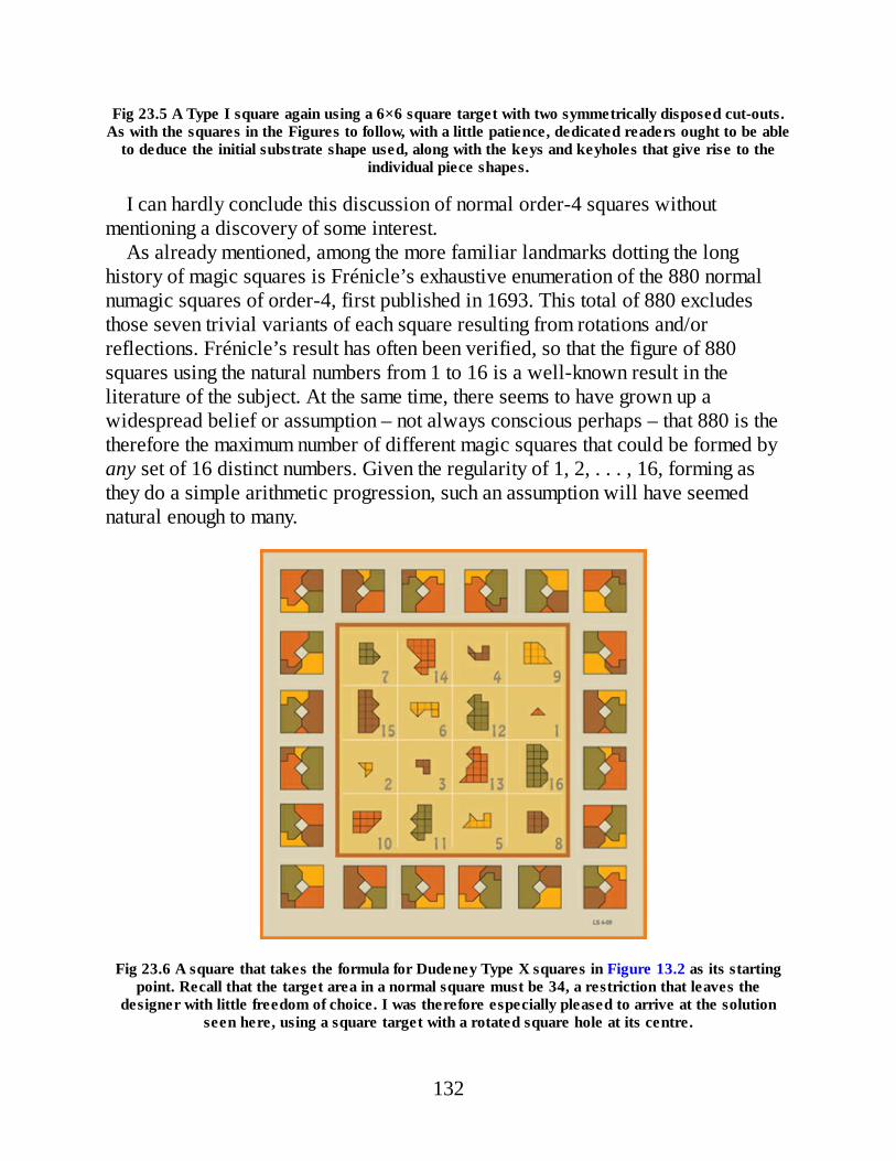
Fig 23.5 A Type I square again using a 6×6 square target with two symmetrically disposed cut-outs.As with the squares in the Figures to follow, with a little patience, dedicated readers ought to be able

to deduce the initial substrate shape used, along with the keys and keyholes that give rise to theindividual piece shapes.

I can hardly conclude this discussion of normal order-4 squares withoutmentioning a discovery of some interest.

As already mentioned, among the more familiar landmarks dotting the longhistory of magic squares is Frénicle’s exhaustive enumeration of the 880 normalnumagic squares of order-4, first published in 1693. This total of 880 excludesthose seven trivial variants of each square resulting from rotations and/orreflections. Frénicle’s result has often been verified, so that the figure of 880squares using the natural numbers from 1 to 16 is a well-known result in theliterature of the subject. At the same time, there seems to have grown up awidespread belief or assumption – not always conscious perhaps – that 880 is thetherefore the maximum number of different magic squares that could be formed byany set of 16 distinct numbers. Given the regularity of 1, 2, . . . , 16, forming asthey do a simple arithmetic progression, such an assumption will have seemednatural enough to many.

Fig 23.6 A square that takes the formula for Dudeney Type X squares in Figure 13.2 as its startingpoint. Recall that the target area in a normal square must be 34, a restriction that leaves the

designer with little freedom of choice. I was therefore especially pleased to arrive at the solutionseen here, using a square target with a rotated square hole at its centre.

132

Fig 23.7 Experimenting with different Types, I took Dudeney’s formula for Type IX as the templatefor this square. ‘The Mazarin Stone’ is the name of a famous yellow diamond that becomes the

subject of a Sherlock Holmes investigation in an Arthur Conan Doyle story of the same name. Thegem-like target shape of area 34 that has been arrived at is celebrated in the picture title.

Fig 23.8 Important as is the choice of template used, one can hardly get far in designing a geomagicsquare before deciding on the target shape. Here, the template used is the formula for Type II in

133

Figure 13.2, which implies a substrate of 16 identical pieces. This in turn calls for a target that can bedissected into 4 congruent pieces, a goal easiest to achieve when the shape chosen has four-fold

rotational symmetry.

Fig 23.9 Four-fold rotational symmetry again underlies the choice of target shape in this square thatis based on the Type III formula in Figure 13.2. As in the analysis of Figure 23.4, the substrate

square consists of 16 identical pieces each with a area of 34 ÷ 4 = 8½. Having decided not to clutterthe cells with numerals, the title ‘Opus 34’ is a sly pointer to the target’s area, and with it to the fact

that piece sizes again form the progresssion 1, 2, 3, . . . .

134

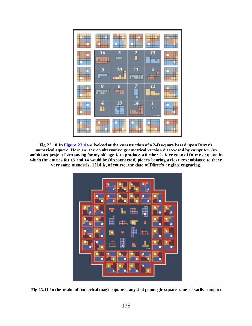
Fig 23.10 In Figure 23.4 we looked at the construction of a 2-D square based upon Dürer’snumerical square. Here we see an alternative geometrical version discovered by computer. An

ambitious project I am saving for my old age is to produce a further 2- D version of Dürer’s square inwhich the entries for 15 and 14 would be (disconnected) pieces bearing a close resemblance to these

very same numerals. 1514 is, of course, the date of Dürer’s original engraving.

Fig 23.11 In the realm of numerical magic squares, any 4×4 panmagic square is necessarily compact

135

and any compact square necessarily panmagic. But not so the world of 2-D magic squares. The 4×4square here is compact but it is not panmagic. Similarly, there exist 2-D squares that are panmagic

without being compact; see, for example, Figure 16.8.

Fig 23.12 A key to Figure 23.11.

Fig 23.13 One of 1040 numagic squares using 1 – 17, but no 9.

However, in 1996, I wrote a computer program able to generate every possible4×4 magic square constructable from any given set of 16 distinct integers. An earlyoutcome of this enterprise showed the above assumption to be untrue. Extensivetrials have revealed the existence of one particular set that yields 1040 rather than880 squares. It is a balanced or ‘palindromic’ set of integers that do not form anarithmetic progression: – 8, – 7, . . . , –1, 1, 2, . . . 8. Note the absence of zero. Thevalue of the new magic sum is also zero. Being built up from 8 complementarypairs (each of which again sum to zero), these 1,040 squares can again beclassified in terms of Dudeney Types, the number of squares of each Type being asseen in Table 5.

136

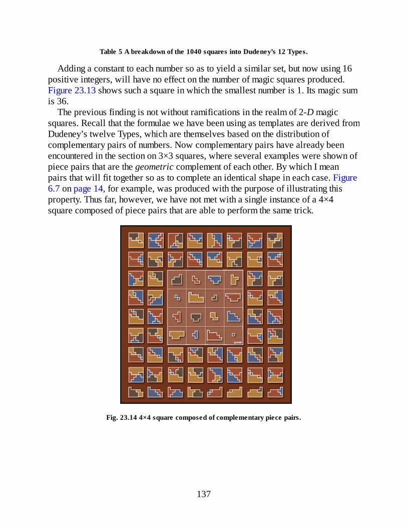
Table 5 A breakdown of the 1040 squares into Dudeney’s 12 Types.

Adding a constant to each number so as to yield a similar set, but now using 16positive integers, will have no effect on the number of magic squares produced.Figure 23.13 shows such a square in which the smallest number is 1. Its magic sumis 36.

The previous finding is not without ramifications in the realm of 2-D magicsquares. Recall that the formulae we have been using as templates are derived fromDudeney’s twelve Types, which are themselves based on the distribution ofcomplementary pairs of numbers. Now complementary pairs have already beenencountered in the section on 3×3 squares, where several examples were shown ofpiece pairs that are the geometric complement of each other. By which I meanpairs that will fit together so as to complete an identical shape in each case. Figure6.7 on page 14, for example, was produced with the purpose of illustrating thisproperty. Thus far, however, we have not met with a single instance of a 4×4square composed of piece pairs that are able to perform the same trick.

Fig. 23.14 4×4 square composed of complementary piece pairs.

137

Fig. 23.15 A square similar to Figure 23.14 but now with circular targets.

I have to admit that, for reasons as yet obscure, attempts to produce a normalsquare with this property have not met with success. However, in Figures 23.14and 23.15 can be seen two such examples based not upon normal numagics but onFig 23.13, which is one among the 1040 squares that can be formed using thenumbers 1 to 17, excepting 9. The two figures are exact analogues, their onlydifferences lying in the choice of piece and target shapes. In both, the 16 pieces arecomposed of 8 complementary pairs. Every pair tiles an identical shape that isone-half of the target. The pairs can be seen in the bottom row of figures, any twoof which will combine to complete the target. In all, there are 52 groups of fourtarget-tiling pieces, only 48 of which are shown. The remaining four can beassembled using the four corner pieces belonging to each of the four embedded 3×3sub-squares. It can be shown that these same sets of 16 pieces admit ofrearrangements yielding a total of 528 distinct 2-D squares, rotations andreflections not counted. A key to both Figures can be seen in Figure 23.16.

Four distinct 4×4 geomagic squares occupy the corners of ‘Art of Fugue’ inFigure 23.17: one yellow, one blue, one orange, and one brown. All four squaresare both nasik and compact. The set of sixteen pieces used is the same in each case.Although not immediately apparent, they comprise eight pairs, each of which willagain combine to tile an identical shape that is half the target. At the centre of thepicture, slightly enlarged copies of the four corner squares (minus their targets) areshown superimposed, their pieces now revealed as exactly coinciding with each

138

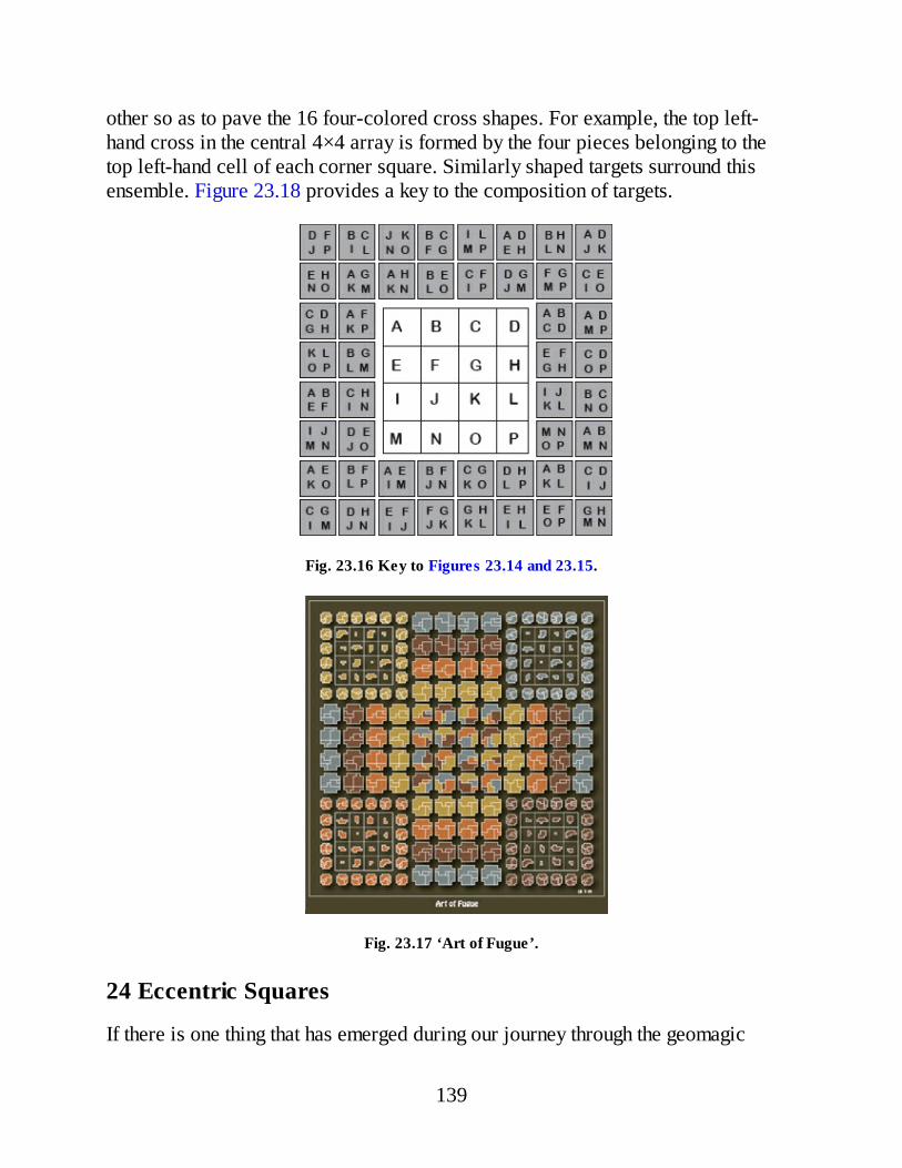
other so as to pave the 16 four-colored cross shapes. For example, the top left-hand cross in the central 4×4 array is formed by the four pieces belonging to thetop left-hand cell of each corner square. Similarly shaped targets surround thisensemble. Figure 23.18 provides a key to the composition of targets.

Fig. 23.16 Key to Figures 23.14 and 23.15.

Fig. 23.17 ‘Art of Fugue’.

24 Eccentric Squares

If there is one thing that has emerged during our journey through the geomagic

139

jungle it is that the local fauna is far more variegated than that met with in the realmof numerical magic squares. It is not just that the lions and tigers hereabouts aremore colorful and roar louder; there exist creatures in Flatland that have nocounterpart in a one-dimensional world. As a result, 2-D magic squares are notalways easy to classify in terms of established categories. This can createproblems for the author bent on presenting a coherent account, whose onlyremaining course is to set out his stall and hope for the best. To this end, in thefollowing I present a selection of special finds that are obviously worthy ofattention, if difficult to place within in a logical scheme.

A good title for Figure 24.1 might be ‘Binary Star’, because the starry bluestructure at the centre of the square can be interpreted as a 3×3 array in twodifferent ways:

As the targets show, both are 3×3 geomagic squares. Note that this ambitiousgoal has been achieved at a price. The pieces used are all pentominoes, someconnected, but mostly weakly-connected or completely disconnected. Naturally, Iwould have preferred them all to be connected, but no such solution could befound. Likewise, the target shape is not all that desire would wish. Nevertheless,the square is a nice instance of the more potent magic structures that can be foundin the world of two dimensions.

140

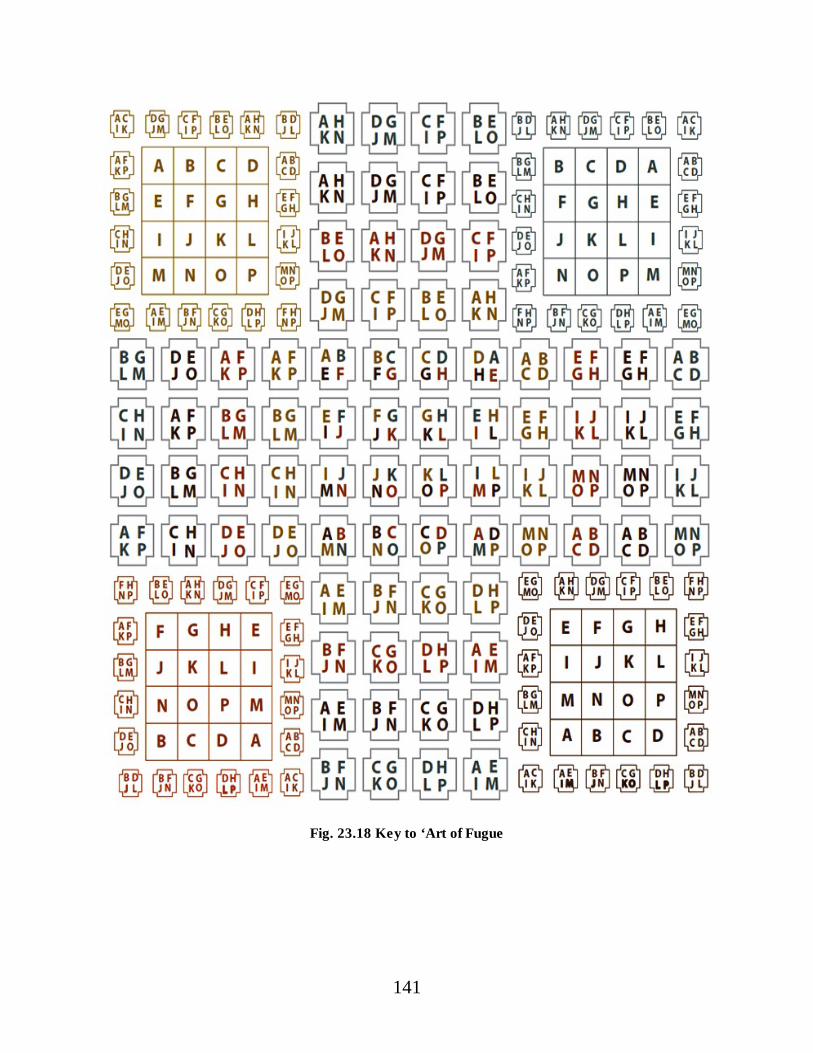
Fig. 23.18 Key to ‘Art of Fugue

141

Fig. 24.1 ‘Binary Star:’ two geomagic squares in one.

Previously I mentioned lions and tigers, but these are not the only animalsroaming the forest. Figure 24.2, ‘Genetic Engineering,’ shows a swarm ofbutterflies collected amid the same woodland glades. Together with the picture tofollow, this square celebrates a breakthrough. In creating a geomagic square, thechoice of admissible target shapes is usually tightly constrained. Scrutiny willshow that the target here is essentially a simple chain of four pieces. But two of thepieces, both yellow, always occur at the ends of the chain, which means they canbe extended so as to take on almost any shape, without introducing deleterious sideeffects. Here they have been extended so as to meet, and so completely envelopethe chain itself, the shape of their combined outline then being entirely up to theconstructor. The choice of a butterfly struck me as an improvement over that of thetriangle used in Figure 11.8 (‘Indian Reservation’) on page 38, which embodies thesame principle of construction.

142

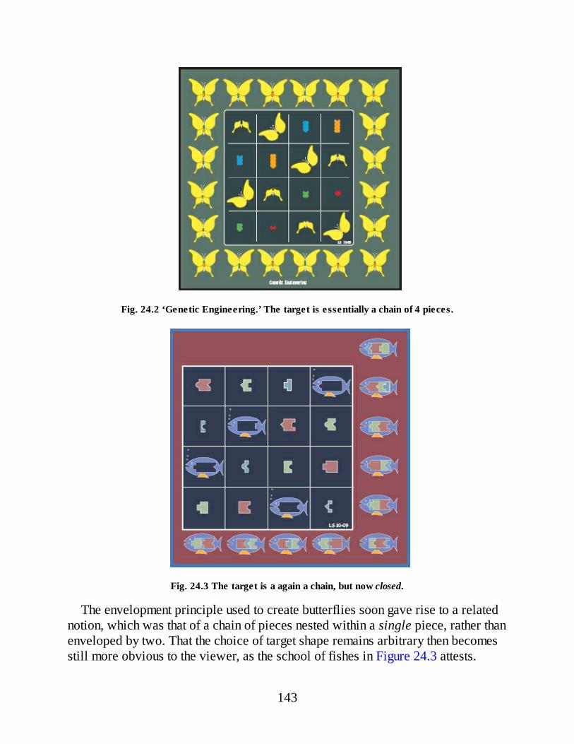
Fig. 24.2 ‘Genetic Engineering.’ The target is essentially a chain of 4 pieces.

Fig. 24.3 The target is a again a chain, but now closed.

The envelopment principle used to create butterflies soon gave rise to a relatednotion, which was that of a chain of pieces nested within a single piece, rather thanenveloped by two. That the choice of target shape remains arbitrary then becomesstill more obvious to the viewer, as the school of fishes in Figure 24.3 attests.

143

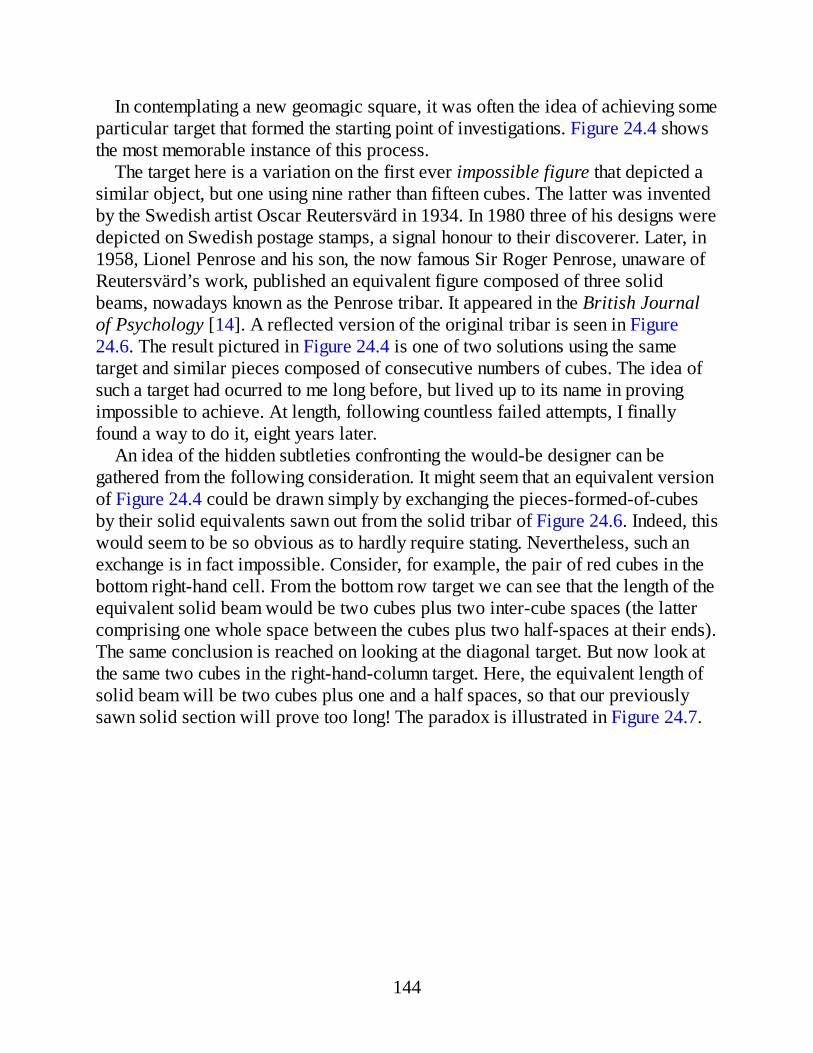
In contemplating a new geomagic square, it was often the idea of achieving someparticular target that formed the starting point of investigations. Figure 24.4 showsthe most memorable instance of this process.

The target here is a variation on the first ever impossible figure that depicted asimilar object, but one using nine rather than fifteen cubes. The latter was inventedby the Swedish artist Oscar Reutersvärd in 1934. In 1980 three of his designs weredepicted on Swedish postage stamps, a signal honour to their discoverer. Later, in1958, Lionel Penrose and his son, the now famous Sir Roger Penrose, unaware ofReutersvärd’s work, published an equivalent figure composed of three solidbeams, nowadays known as the Penrose tribar. It appeared in the British Journalof Psychology [14]. A reflected version of the original tribar is seen in Figure24.6. The result pictured in Figure 24.4 is one of two solutions using the sametarget and similar pieces composed of consecutive numbers of cubes. The idea ofsuch a target had ocurred to me long before, but lived up to its name in provingimpossible to achieve. At length, following countless failed attempts, I finallyfound a way to do it, eight years later.

An idea of the hidden subtleties confronting the would-be designer can begathered from the following consideration. It might seem that an equivalent versionof Figure 24.4 could be drawn simply by exchanging the pieces-formed-of-cubesby their solid equivalents sawn out from the solid tribar of Figure 24.6. Indeed, thiswould seem to be so obvious as to hardly require stating. Nevertheless, such anexchange is in fact impossible. Consider, for example, the pair of red cubes in thebottom right-hand cell. From the bottom row target we can see that the length of theequivalent solid beam would be two cubes plus two inter-cube spaces (the lattercomprising one whole space between the cubes plus two half-spaces at their ends).The same conclusion is reached on looking at the diagonal target. But now look atthe same two cubes in the right-hand-column target. Here, the equivalent length ofsolid beam will be two cubes plus one and a half spaces, so that our previouslysawn solid section will prove too long! The paradox is illustrated in Figure 24.7.

144

Fig. 24.4 An interesting case. But is it a geomagic square?

Fig. 24.5 A geomagic square. But is it an interesting case?

145

Fig. 24.6 Penrose Tribar, but can it replace the cubes in Figure 24.4?

Some might say that Figure 24.4 is not really a geomagic square at all, becausethe target does not really exist. Nor will it help if the pieces are viewed as two-dimensional, rather than as the 3-D objects they suggest. Scrutiny will show thatpiece outlines in targets often differ slightly from the outline of the same piece inits cell, so that we are not even dealing with a legitimate 2-D case. Nevertheless,that a true geomagic square does indeed underlie the tribar square is made evidentin Figure 24.5, in which polyhexes replace cubes. Here the title ‘Truth and Beauty’was suggested by the compelling logic and simple elegance of the solution.

Fig. 24.7 The dots work but the strips don’t. Why?

As described previously in this account, among other enticing prospectscompeting for attention during the early days of research was the notion of ageomagic square able to tile two different targets. A fond dream in a golden mist,as it then seemed. Thereafter we looked at the work of Thoen, de Meulenmeesterand Postl, with their amazing 3×3 specimen that surpasses every expectation inachieving the same goal with as many as twelve distinct targets. Surely here was a

146

record it would be naïve to try to improve upon. Nevertheless, the square shown inFigure 24.7 not only succeeds in this, it even does so by a comfortable margin.

Figure 24.8 is in fact a 4×4 semimagic square, which is to say, a square that ismagic along rows and columns only. However, the square has a redeeming factor inthat its target may take an infinite range of different forms. Each of the fourquadrants is a 2×2 semimagic square showing identical ‘half-targets.’ The fourpieces in each row and column can thus tile any region, connected or disconnected,that is a union of two such half-targets, irrespective of their spatial relation toeach other. In this way, the possible target shapes are simply unlimited in variety.

For all that, there is no getting around the fact that Figure 24.8 is not fully magic.Moreover, there is not a single piece that is not either weakly-connected ordisjoint. Spurred on by these blemishes, the pursuit for perfection was rejoined andeventually crowned with success. The 6×6 square in Figure 24.9 surmounts bothshortcomings while again enabling an infinite variety of possible target shapes. Thelatter are again formed by the union of two identical halves. Here, each of the fourquadrants is a 3×3 almost-magic square (only one magic diagonal), all sharing acommon half-target shape.

Fig. 24.8 A semi-magic square, but with a redeeming factor.

No discussion of remarkable specimens in this field can overlook two furthercontributions from the discoverer of the very first order-2 geomagic square, FrankTinkelenberg. In the first place is his beautiful geomagic star seen in Figure 24.10.Frank ought to change his name to Twinkelenberg. It was a prize-winning entry in a

147

competion held by Matthijs Coster in the Dutch periodical Pythagoras [15][16].Note the thought that has gone into his choice of target. Assuming consecutively-sized pieces, its area had to be 33, a number that rules out shapes showing six-foldrotational symmetry. Even so, the hexagonal symmetry of the star is strikingly re-echoed by the hole at the target’s centre. Secondly, wielding anew his novelconstruction principle, originally applied to order-2, Frank then turned to order-3.Figure 24.11 shows his extraordinary find that breaks all previous records for 3×3magic squares. To begin with, it is a 3×3 panmagic square, which accounts for 12of the 28 targets shown. The remaining 16 targets are formed by every 4 triads ofpieces that can be chosen from any 2×2 subsquare. One seeing is worth a thousandwords. Frank tells me that the same nine pieces tile the target in 62 different ways.These nine pieces are a subset chosen from among twelve pieces, using which thetarget can be formed in 148 different ways. My guess is that records will again beshattered once this same technique is applied to 4×4 squares. Hats off to a greatachievement!

Fig. 24.9 A 6×6 square able to tile an infinite number of distinct targets.

148

Fig. 24.10 A geomagic star.

Fig. 24.11 A record-breaking 3×3 geomagic square.

25 Collinear Collations

The geomagic construction I would like to discuss last is so peculiar as to requirea digression.

Martin Gardner once introduced the Lo shu with the words, “To appreciate thegem-like beauty of this most ancient of all combinatorial curiosities, consider allthe ways that its constant, 15, can be partitioned into a triplet of distinct positiveintegers. There are exactly eight:

149

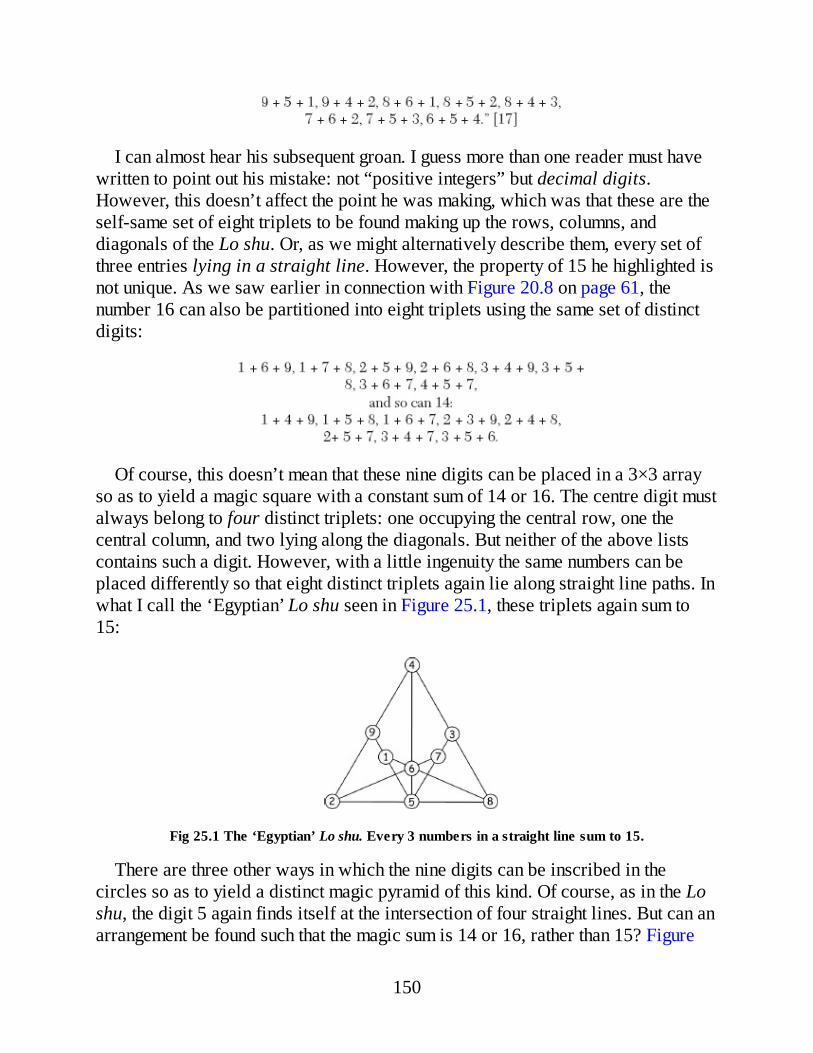
I can almost hear his subsequent groan. I guess more than one reader must havewritten to point out his mistake: not “positive integers” but decimal digits.However, this doesn’t affect the point he was making, which was that these are theself-same set of eight triplets to be found making up the rows, columns, anddiagonals of the Lo shu. Or, as we might alternatively describe them, every set ofthree entries lying in a straight line. However, the property of 15 he highlighted isnot unique. As we saw earlier in connection with Figure 20.8 on page 61, thenumber 16 can also be partitioned into eight triplets using the same set of distinctdigits:

Of course, this doesn’t mean that these nine digits can be placed in a 3×3 arrayso as to yield a magic square with a constant sum of 14 or 16. The centre digit mustalways belong to four distinct triplets: one occupying the central row, one thecentral column, and two lying along the diagonals. But neither of the above listscontains such a digit. However, with a little ingenuity the same numbers can beplaced differently so that eight distinct triplets again lie along straight line paths. Inwhat I call the ‘Egyptian’ Lo shu seen in Figure 25.1, these triplets again sum to15:

Fig 25.1 The ‘Egyptian’ Lo shu. Every 3 numbers in a straight line sum to 15.

There are three other ways in which the nine digits can be inscribed in thecircles so as to yield a distinct magic pyramid of this kind. Of course, as in the Loshu, the digit 5 again finds itself at the intersection of four straight lines. But can anarrangement be found such that the magic sum is 14 or 16, rather than 15? Figure

150

25.2, the ‘Venusian’ Lo shu, arrived at after some trial and error, supplies ananswer; its magic sum is 16. Replacing each digit d with 10–d, results in a similarsolution showing a magic sum of 14. It is not difficult to show that for the eighttriplets to share the same total then the nine numbers must always form anarithmetic progression.

Fig 25.2 The ‘Venusian’ Lo shu. Every 3 numbers in a straight line sum to 16.

It was while exploring such systems of collinear triads that I noticed how thenine points could be chosen so as to coincide with the centres of the cells in a 7×7square array. Soon after, I turned up a similar specimen in which the array was5×5. Could a yet smaller example be found? A decisive step was to drop therequirement that points need coincide with cell centres, so long as they fell withincells. In this way, by degrees I arrived at the specimen of 4×4 seen in Figure 25.3,a result that finally jolted me into the realization of what one further step down insize would entail. For the nine points would then occupy all nine cells of a 3×3array, a result with mischievous potential. With this goal in sight, I thus spared noeffort in a diligent search for a solution. On succeeding, the latter then formed thebasis for a new puzzle that has been described as ‘devilish’ [18]. It can be seen inFigure 25.4.

Fig 25.3 right collinear triads, the numbered points now falling within the cells of a 4×4 array.

In the diagram below, nine numbered counters occupy the cells of a 3x3 checkerboard so as to form a magicsquare. Any 3 counters lying in a straight line add up to 15. There are 8 of these collinear triads.

151

Reposition the counters (again, one to each cell) to yield 8 new collinear triads, but now showing a commonsum of 16 rather than 15.

Fig 25.4 A seemingly impossibe challenge?

Fig 25.5 One solution among others.

152

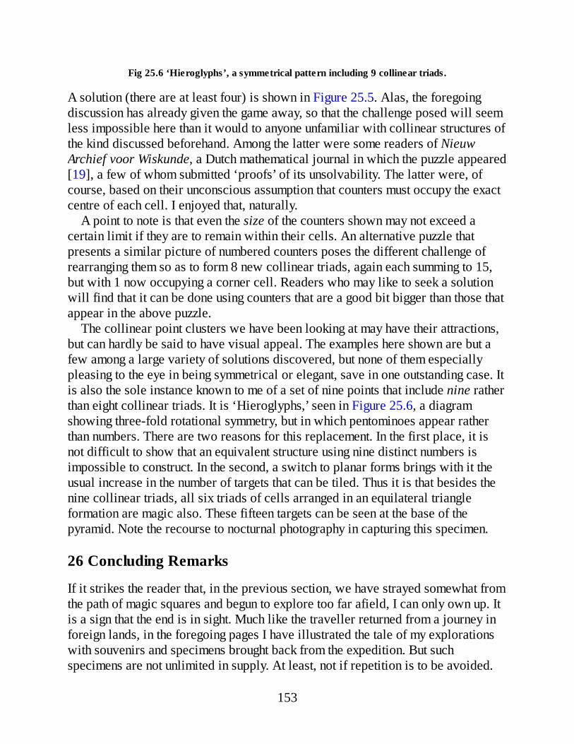
Fig 25.6 ‘Hieroglyphs’, a symmetrical pattern including 9 collinear triads.

A solution (there are at least four) is shown in Figure 25.5. Alas, the foregoingdiscussion has already given the game away, so that the challenge posed will seemless impossible here than it would to anyone unfamiliar with collinear structures ofthe kind discussed beforehand. Among the latter were some readers of NieuwArchief voor Wiskunde, a Dutch mathematical journal in which the puzzle appeared[19], a few of whom submitted ‘proofs’ of its unsolvability. The latter were, ofcourse, based on their unconscious assumption that counters must occupy the exactcentre of each cell. I enjoyed that, naturally.

A point to note is that even the size of the counters shown may not exceed acertain limit if they are to remain within their cells. An alternative puzzle thatpresents a similar picture of numbered counters poses the different challenge ofrearranging them so as to form 8 new collinear triads, again each summing to 15,but with 1 now occupying a corner cell. Readers who may like to seek a solutionwill find that it can be done using counters that are a good bit bigger than those thatappear in the above puzzle.

The collinear point clusters we have been looking at may have their attractions,but can hardly be said to have visual appeal. The examples here shown are but afew among a large variety of solutions discovered, but none of them especiallypleasing to the eye in being symmetrical or elegant, save in one outstanding case. Itis also the sole instance known to me of a set of nine points that include nine ratherthan eight collinear triads. It is ‘Hieroglyphs,’ seen in Figure 25.6, a diagramshowing three-fold rotational symmetry, but in which pentominoes appear ratherthan numbers. There are two reasons for this replacement. In the first place, it isnot difficult to show that an equivalent structure using nine distinct numbers isimpossible to construct. In the second, a switch to planar forms brings with it theusual increase in the number of targets that can be tiled. Thus it is that besides thenine collinear triads, all six triads of cells arranged in an equilateral triangleformation are magic also. These fifteen targets can be seen at the base of thepyramid. Note the recourse to nocturnal photography in capturing this specimen.

26 Concluding Remarks

If it strikes the reader that, in the previous section, we have strayed somewhat fromthe path of magic squares and begun to explore too far afield, I can only own up. Itis a sign that the end is in sight. Much like the traveller returned from a journey inforeign lands, in the foregoing pages I have illustrated the tale of my explorationswith souvenirs and specimens brought back from the expedition. But suchspecimens are not unlimited in supply. At least, not if repetition is to be avoided.

153

Time thus to bring this account to a close before such an accusation can belevelled. I conclude with a few parting observations.

It may have been noticed that, with a single exception, magic squares larger than4×4 have escaped attention in the foregoing account. The reason is simply thatlarger squares have seldom struck me as attractive. How many readers are going tobe tempted to add up swarms of numbers in order to verify that a square is magic?A dedicated few only, I cannot help thinking. And what then of the elegance that isthe very hallmark of the (small) magic square? Similar reservations apply to non-numerical squares. Moreover, it is a common fallacy that the bigger the square, thegreater the achievement it represents, because of the supposed difficulty of gettingso many numbers to comply with the magic conditions. But this idea is quite simplymistaken. It is easily shown that the constraints imposed in fact diminish withincreasing size of square. For, as Chernick [20] was the first to prove, an algebraicgeneralization of an N × N numerical magic square can always be written so thatN2 – 2N of its cells are each occupied by a single independent variable. Or inlayman’s terms: in creating a magic square of order-N, the proportion of cells thatcan be assigned any desired number is 1 – 2/N, a proportion that increases with N,and is already as much as two-thirds of the cells for a square of size 6×6.

These ruminations are a reminder of a related question. I refer to the problem ofhow the ‘magicality’ of a square is to be assessed. The question receives next to noconsideration in the literature, and yet the matter of what makes one magic squaremore magic, and hence more praiseworthy than another, is really of centralimportance to the whole topic. Magic-square buffs are at heart trophy-hunters, theessence of the game being to track down new specimens that outclass theopponent’s bag. But how, in the absence of yardsticks or scales, are meaningfulcomparisons to be made among different exhibits? That there is no easy answer tothe question is to be seen by considering the case of that most famous square of all,the universally acclaimed Lo shu.

What do we find when we look at the numbers appearing in the Lo shu whenpictured as a collection of points distributed along the real number line? Theanswer is shown in Figure 26.1. It is a set of nine equidistant points positionedslightly to the right of zero, which is at the origin, or centre of the line.

But what kind of an aesthetically insensitive soul, I wonder, has left this peerlessstring of pearls lying carelessly in such an asymmetrical position? And why hasthe right- hand side of the line been chosen over the left? Is this not blatant signism,a form of discrimination against negative numbers?

Oh come now, I hear a critic rejoin, what possible difference can the position ofthe nine points make? Their key property is that they form an arithmeticprogression, which is to say, they form a chain of equidistant links. Placing them

154

where they are yields us a magic square that contains the first nine countingnumbers, which are simple, pleasing, and immediately recognized by all. Lay themanywhere else and the result will be an essentially identical magic square but onelacking in these desirable qualities. And in any case, can any better position on theline be found?

Fig. 26.1 A string of pearls.

Fig. 26.2 The balanced square and its close relative the LO shu.

It can. When it comes to magic squares, symmetry and magicality are the twosides of a single coin. Increase one and the other will be augmented. Decrease oneand the other will diminish. As we shall see, the asymmetrical position of thepoints used in the Lo shu exacts a price that is paid for through a relative reductionin its magical properties.

To see this, let us slide our set of equidistant points leftwards along the line tothe only position of true balance or symmetry, which is in the exact centre. Thecentral number of the progression now coincides with zero, and the result is the‘balanced’ magic square of Figure 26.2 (left), whose simplicity may belie itsenhanced magicality. For comparison, the Lo shu appears at right.

To begin with, consider the sum of the four corner numbers in the Lo shu. It is 2+ 4 + 6 + 8 = 20. In our new square it is -3 + -1 + 1 + 3 = 0, the same value as thecentre number. Or in other words, the centre number is equal to the sum of its fourimmediate diagonal neighbours. But now consider both squares as if toroidally-connected. The four diagonal neighbours of any cell are then the same as theywould be were the square used as a tile with which to cover the plane. This bringsto light an arresting fact. For, unlike the Lo shu, every entry in the left-hand squareis now found to be equal to the sum of its four diagonal neighbours.

Now is that not a ‘magical’ property to celebrate? Had the same thing been true

155

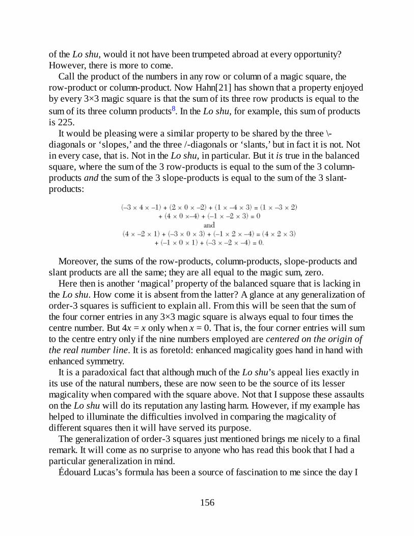
of the Lo shu, would it not have been trumpeted abroad at every opportunity?However, there is more to come.

Call the product of the numbers in any row or column of a magic square, therow-product or column-product. Now Hahn[21] has shown that a property enjoyedby every 3×3 magic square is that the sum of its three row products is equal to thesum of its three column products8. In the Lo shu, for example, this sum of productsis 225.

It would be pleasing were a similar property to be shared by the three \-diagonals or ‘slopes,’ and the three /-diagonals or ‘slants,’ but in fact it is not. Notin every case, that is. Not in the Lo shu, in particular. But it is true in the balancedsquare, where the sum of the 3 row-products is equal to the sum of the 3 column-products and the sum of the 3 slope-products is equal to the sum of the 3 slant-products:

Moreover, the sums of the row-products, column-products, slope-products andslant products are all the same; they are all equal to the magic sum, zero.

Here then is another ‘magical’ property of the balanced square that is lacking inthe Lo shu. How come it is absent from the latter? A glance at any generalization oforder-3 squares is sufficient to explain all. From this will be seen that the sum ofthe four corner entries in any 3×3 magic square is always equal to four times thecentre number. But 4x = x only when x = 0. That is, the four corner entries will sumto the centre entry only if the nine numbers employed are centered on the origin ofthe real number line. It is as foretold: enhanced magicality goes hand in hand withenhanced symmetry.

It is a paradoxical fact that although much of the Lo shu’s appeal lies exactly inits use of the natural numbers, these are now seen to be the source of its lessermagicality when compared with the square above. Not that I suppose these assaultson the Lo shu will do its reputation any lasting harm. However, if my example hashelped to illuminate the difficulties involved in comparing the magicality ofdifferent squares then it will have served its purpose.

The generalization of order-3 squares just mentioned brings me nicely to a finalremark. It will come as no surprise to anyone who has read this book that I had aparticular generalization in mind.

Édouard Lucas’s formula has been a source of fascination to me since the day I

156

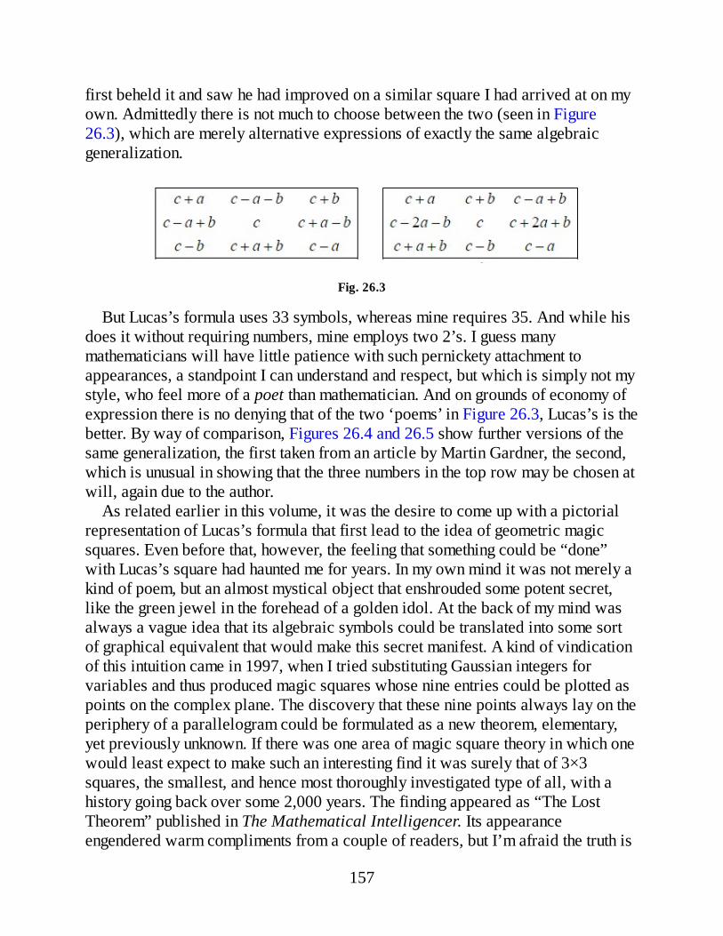
first beheld it and saw he had improved on a similar square I had arrived at on myown. Admittedly there is not much to choose between the two (seen in Figure26.3), which are merely alternative expressions of exactly the same algebraicgeneralization.

Fig. 26.3

But Lucas’s formula uses 33 symbols, whereas mine requires 35. And while hisdoes it without requiring numbers, mine employs two 2’s. I guess manymathematicians will have little patience with such pernickety attachment toappearances, a standpoint I can understand and respect, but which is simply not mystyle, who feel more of a poet than mathematician. And on grounds of economy ofexpression there is no denying that of the two ‘poems’ in Figure 26.3, Lucas’s is thebetter. By way of comparison, Figures 26.4 and 26.5 show further versions of thesame generalization, the first taken from an article by Martin Gardner, the second,which is unusual in showing that the three numbers in the top row may be chosen atwill, again due to the author.

As related earlier in this volume, it was the desire to come up with a pictorialrepresentation of Lucas’s formula that first lead to the idea of geometric magicsquares. Even before that, however, the feeling that something could be “done”with Lucas’s square had haunted me for years. In my own mind it was not merely akind of poem, but an almost mystical object that enshrouded some potent secret,like the green jewel in the forehead of a golden idol. At the back of my mind wasalways a vague idea that its algebraic symbols could be translated into some sortof graphical equivalent that would make this secret manifest. A kind of vindicationof this intuition came in 1997, when I tried substituting Gaussian integers forvariables and thus produced magic squares whose nine entries could be plotted aspoints on the complex plane. The discovery that these nine points always lay on theperiphery of a parallelogram could be formulated as a new theorem, elementary,yet previously unknown. If there was one area of magic square theory in which onewould least expect to make such an interesting find it was surely that of 3×3squares, the smallest, and hence most thoroughly investigated type of all, with ahistory going back over some 2,000 years. The finding appeared as “The LostTheorem” published in The Mathematical Intelligencer. Its appearanceengendered warm compliments from a couple of readers, but I’m afraid the truth is

157

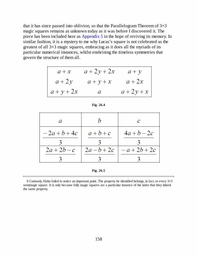
that it has since passed into oblivion, so that the Parallelogram Theorem of 3×3magic squares remains as unknown today as it was before I discovered it. Thepiece has been included here as Appendix 5 in the hope of reviving its memory. Insimilar fashion, it is a mystery to me why Lucas’s square is not celebrated as thegreatest of all 3×3 magic squares, embracing as it does all the myriads of itsparticular numerical instances, whilst enshrining the timeless symmetries thatgovern the structure of them all.

Fig. 26.4

Fig. 26.5

8 Curiously, Hahn failed to notice an important point. The property he identified belongs, in fact, to every 3×3semimagic square. It is only because fully magic squares are a particular instance of the latter that they inheritthe same property.

158

Appendix I

A Formal Definition of Geomagic Squares

An informal definition of geomagic squares has been given elsewhere in this book.From the mathematical point of view, however, loose talk about ‘pieces fittingtogether as in a jigsaw’ is clearly inadequate. The purpose of this addendum is thusto provide a formal definition of geomagic squares. To this end, we begin bydefining a ‘generic’ magic square, by which is intended a generalized magic squarein its widest possible sense. That is, a canonical magic square is described, butwithout stipulating the kind of ‘objects’ that occupy its cells, and without specifyinghow these combine so as to form a constant target (‘target’ again in the broadestsense possible).

Although the presentation has been kept as informal as possible, a degree offormality is necessary. No doubt some mathematicians will find the treatment toolax; for laymen it may prove too demanding. At the same time, certain details haveinevitably escaped mention, just as some of the mathematical concepts involvedcould have been explained more fully

Properties of the Generic Magic Square

Fundamental to any conceivable magic square (of order n ≥ 2) is an n × n matrix Mover a domain D, in which we discern 2n + 2 (potentially ‘magic’) lines: the nrows, the n columns, the main diagonal (\) and the co-diagonal (/).

All essential properties of the generic square of order n ≥ 2 can now bespecified in a list of 5 components:

i) A domain D, which is a set of ‘objects’ that will occupy the cells of M. In the case of numerical magicsquares, this domain would be simply the ring of integers Z.

ii) A binary operation + on D. Since the n objects in every line must be able to merge so as to form the same‘sum’ in each case, we require that D be equipped with a rule of combination. Our requirements will be metby a binary operation + that is:

commutative (d1, + d2 = d2 + d1), associative d1 + (d2 + d3) = (d1 + d2) + d3, and has an identityelement ‘0,’ such that 0 + d = d + 0 = d for all d D.

We shall use the term ‘sum’ for the operation +. For D = Z the binary operation isordinary addition and the identity element is zero.

iii) An equivalence relation ~ on D. For D = Z this equivalence relation is equality (‘=’). Note that compatibility

159

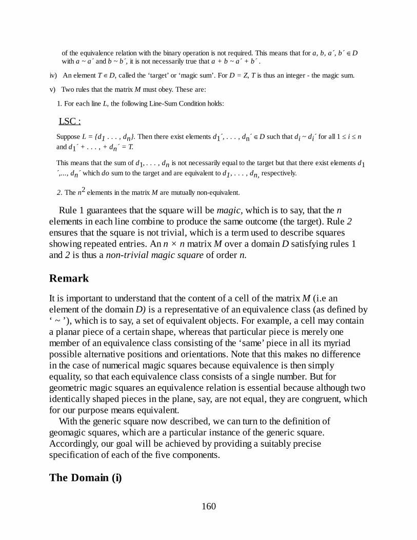
of the equivalence relation with the binary operation is not required. This means that for a, b, a´, b´ Dwith a ~ a´ and b ~ b´, it is not necessarily true that a + b ~ a´ + b´ .

iv) An element T D, called the ‘target’ or ‘magic sum’. For D = Z, T is thus an integer - the magic sum.

v) Two rules that the matrix M must obey. These are:

1. For each line L, the following Line-Sum Condition holds:

LSC :Suppose L = {d1 . . . , dn}. Then there exist elements d1´, . . . , dn´ D such that di ~ di´ for all 1 ≤ i ≤ nand d1´ + . . . , + dn´ = T.

This means that the sum of d1, . . . , dn is not necessarily equal to the target but that there exist elements d1´,..., dn´ which do sum to the target and are equivalent to d1, . . . , dn, respectively.

2. The n2 elements in the matrix M are mutually non-equivalent.

Rule 1 guarantees that the square will be magic, which is to say, that the nelements in each line combine to produce the same outcome (the target). Rule 2ensures that the square is not trivial, which is a term used to describe squaresshowing repeated entries. An n × n matrix M over a domain D satisfying rules 1and 2 is thus a non-trivial magic square of order n.

Remark

It is important to understand that the content of a cell of the matrix M (i.e anelement of the domain D) is a representative of an equivalence class (as defined by‘ ~ ’), which is to say, a set of equivalent objects. For example, a cell may containa planar piece of a certain shape, whereas that particular piece is merely onemember of an equivalence class consisting of the ‘same’ piece in all its myriadpossible alternative positions and orientations. Note that this makes no differencein the case of numerical magic squares because equivalence is then simplyequality, so that each equivalence class consists of a single number. But forgeometric magic squares an equivalence relation is essential because although twoidentically shaped pieces in the plane, say, are not equal, they are congruent, whichfor our purpose means equivalent.

With the generic square now described, we can turn to the definition ofgeomagic squares, which are a particular instance of the generic square.Accordingly, our goal will be achieved by providing a suitably precisespecification of each of the five components.

The Domain (i)

160

By way of introduction to the domain to be used, consider closed, bounded subsetsof the Euclidean space of dimension d (d ≥ 1). A subset C is ‘closed’ if and only ifall boundary points of C belong to C. An example is the unit disk, which consists ofall points of the plane having distance ≤ 1 from the origin. It is a closed set becauseits boundary, the unit circle, belongs entirely to it. If we remove any number ofpoints from the boundary (the unit circle) then the resulting set is no longer closed.

Further, a subset B is ‘bounded’ if and only if there exists a sphere of sufficientlylarge radius such that B is completely surrounded by it. In other words, B does not‘extend to infinity’ in any direction. Subsets of Euclidean spaces, which are bothclosed and bounded are known as ‘compact’ subsets. In fact, in general topology,the definition of ‘compact’ is different, but in the special case of Euclidean spacesthe two definitions are equivalent, so that ‘compact = closed + bounded’, as shownby the Heine-Borel theorem. In light of these remarks, our domain D will be the setof all compact subsets of Euclidean space of dimension d (d ≥ 1). Hence, by ageomagic square of dimension d will be meant one in which every entry is acompact subset of the Euclidean space of dimension d.

The remaining 4 components can now be identified as follows:

The Binary Operation (ii)

For two compact subsets A and B of the space, let A + B := A ∪ B (set union). Theidentity element 0 is then the empty set Ø.

The Equivalence Relation (iii)

For two compact subsets A and B of the space, let A ~ B if and only if A and B arecongruent, that is, there exists an invertible, affine linear distance-preservingtransformation h of the space such that h(A) = B.

This means that the set B can be obtained from the set A by a displacement of Athrough space, involving rotations and/or translations, together with a possiblereflection.

The Target (iv)

The target T is any compact subset of the space, that is, a member of D.

The Line-Sum Condition (v)

The two rules to be obeyed by the matrix M remain unchanged for geomagicsquares, although the latter do impose an additional requirement on the Line-Sum

161

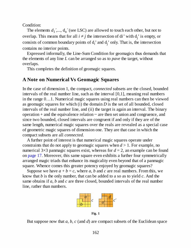
Condition:The elements d1 ,..., dn (see LSC) are allowed to touch each other, but not to

overlap. This means that for all i ≠ j the intersection of di’ with dj’ is empty, orconsists of common boundary points of di’ and dj’ only. That is, the intersectioncontains no interior points.

Expressed informally, the Line-Sum Condition for geomagics thus demands thatthe elements of any line L can be arranged so as to pave the target, withoutoverlaps.

This completes the definition of geomagic squares.

A Note on Numerical Vs Geomagic Squares

In the case of dimension 1, the compact, connected subsets are the closed, boundedintervals of the real number line, such as the interval [0,1], meaning real numbersin the range 0…1. Numerical magic squares using real numbers can then be viewedas geomagic squares for which (i) the domain D is the set of all bounded, closedintervals of the real number line, and (ii) the target is again an interval. The binaryoperation + and the equivalence relation ~ are then set union and congruence, andsince two bounded, closed intervals are congruent if and only if they are of thesame length, numerical magic squares over the reals are revealed as a special caseof geometric magic squares of dimension one. They are that case in which thecompact subsets are all connected.

A further point of interest is that numerical magic squares operate underconstraints that do not apply to geomagic squares when d > 1. For example, nonumerical 3×3 panmagic squares exist, whereas for d = 2, an example can be foundon page 17. Moreover, this same square even exhibits a further four symmetricallyarranged magic triads that enhance its magicality even beyond that of a panmagicsquare. Whence comes this greater potency enjoyed by geomagic squares?

Suppose we have a + b = c, where a, b and c are real numbers. From this, weknow that b is the only number, that can be added to a so as to yield c. And thesame obtains if a, b and c are three closed, bounded intervals of the real numberline, rather than numbers.

Fig. 1

But suppose now that a, b, c (and d) are compact subsets of the Euclidean space

162

of dimension 2 corresponding to the planar pieces seen in Figure 1. Note that a ~ aand c ~ c. But here b is no longer the only piece that can be appended to a so as toyield c. An alternative is the different piece d, because a + b ~ a + d ~ c ~ c. Inshort, the behaviour of compact subsets is inherently more flexible than is that ofnumbers.

Geomagics enjoy more freedom than numerical squares because their targets canbe assembled from members of their domain in many more ways than magic sumscan be formed with numbers.

We have seen that numerical magic squares are a subset of geomagic squares.Could it be that geomagic squares are themselves a subset of some wider genus ofmagic square? The question remains unanswered. In any case, the plethora of newchallenges thrown up by 2-D geomagic squares ought to prove sufficient to keepinvestigators occupied for some time to come.

Grateful thanks are due to my friend Michael Schweitzer who provided themathematical basis of the above definition.

163

Appendix II

Magic Formulae

Introductory Note

Penned in 1980, but never published, ‘Magic Formulae’ was my first ever attemptat writing up a new result in the form of an essay. Knowing little at that time of theworld of professional journals, the style adopted is unusual, my imaginaryaudience being composed of laymen possessed of a smattering of mathematics,such as myself. Thoughts of publication not having been seriously entertained, Isaw myself as my own publisher, and thus took a good deal of trouble over thepresentation, the completed article taking shape as an A5 booklet sandwichedbetween card covers. We didn’t have word-processors in those days, so the wholething was bashed out on my old Adler typewriter, matrices and all. For the frontand back covers, I made drawings of algebraic magic squares in which thevariables were represented by ‘magical’ symbols: runes and astrological signs.The letters used for the title ‘Magic Formulae’ were copied from the Book ofKells. In retrospect I can see that this concern with symbology marked thebeginning of a train of thought that would chug along for some thirty years until itseventual arrival at geometric magic squares. Should anyone be interested in howthe author’s mind works, here then is a good place to start. With the present volumein mind, in the interests of clarity I recently returned to the piece and improved it invarious respects.

164

Algebraic generalizations using runic characters and astrological signs embellished the front andback covers of Magic Formulae. Red symbols stand for positive variables, black symbols for

negative variables. The square at left generalizes panmagics, while the other covers all 4×4 magicsquares.

Magic Formulae

“Runes and charms are very practical formulae designed to procude definiteresults, such as getting a cow out of a bog.”

—T.S. Eliot, The Music of Poetry

In the year 1910, Ernest Bergholt, a familiar name in the British literature onrecreational mathematics of the time, published a new generalization of 4×4 magicsquares [1]. He gives us no clue as to how he arrived at it, but simply presents itwith the claim that “. . . it is the completely general formula . . .”

165

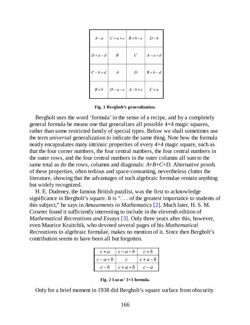
Fig. 1 Bergholt’s generalization.

Bergholt uses the word ‘formula’ in the sense of a recipe, and by a completelygeneral formula he means one that generalizes all possible 4×4 magic squares,rather than some restricted family of special types. Below we shall sometimes usethe term universal generalization to indicate the same thing. Note how the formulaneatly encapsulates many intrinsic properties of every 4×4 magic square, such asthat the four corner numbers, the four central numbers, the four central numbers inthe outer rows, and the four central numbers in the outer columns all sum to thesame total as do the rows, columns and diagonals: A+B+C+D. Alternative proofsof these properties, often tedious and space-consuming, nevertheless clutter theliterature, showing that the advantages of such algebraic formulae remain anythingbut widely recognized.

H. E. Dudeney, the famous British puzzlist, was the first to acknowledgesignificance in Bergholt’s square. It is “. . . of the greatest importance to students ofthis subject,” he says in Amusements in Mathematics [2]. Much later, H. S. M.Coxeter found it sufficiently interesting to include in the eleventh edition ofMathematical Recreations and Essays [3]. Only three years after this, however,even Maurice Kraitchik, who devoted several pages of his MathematicalRecreations to algebraic formulae, makes no mention of it. Since then Bergholt’scontribution seems to have been all but forgotten.

Fig. 2 Lucas’ 3×3 formula.

Only for a brief moment in 1938 did Bergholt’s square surface from obscurity

166

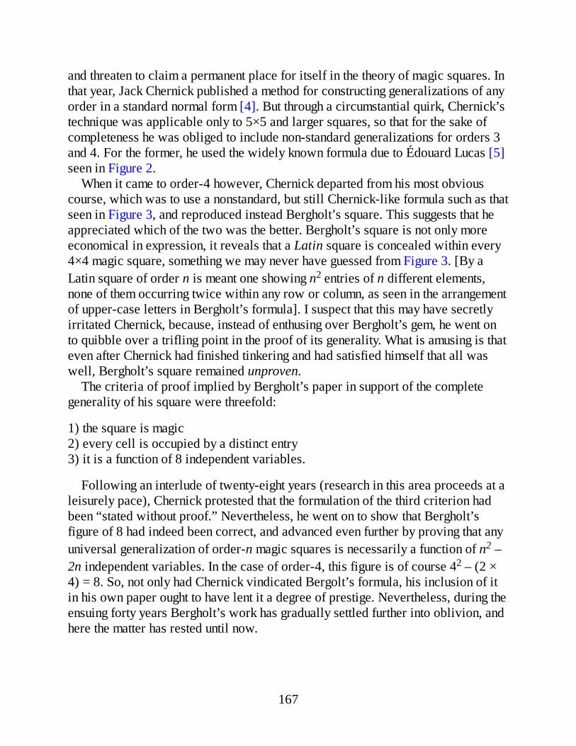
and threaten to claim a permanent place for itself in the theory of magic squares. Inthat year, Jack Chernick published a method for constructing generalizations of anyorder in a standard normal form [4]. But through a circumstantial quirk, Chernick’stechnique was applicable only to 5×5 and larger squares, so that for the sake ofcompleteness he was obliged to include non-standard generalizations for orders 3and 4. For the former, he used the widely known formula due to Édouard Lucas [5]seen in Figure 2.

When it came to order-4 however, Chernick departed from his most obviouscourse, which was to use a nonstandard, but still Chernick-like formula such as thatseen in Figure 3, and reproduced instead Bergholt’s square. This suggests that heappreciated which of the two was the better. Bergholt’s square is not only moreeconomical in expression, it reveals that a Latin square is concealed within every4×4 magic square, something we may never have guessed from Figure 3. [By aLatin square of order n is meant one showing n2 entries of n different elements,none of them occurring twice within any row or column, as seen in the arrangementof upper-case letters in Bergholt’s formula]. I suspect that this may have secretlyirritated Chernick, because, instead of enthusing over Bergholt’s gem, he went onto quibble over a trifling point in the proof of its generality. What is amusing is thateven after Chernick had finished tinkering and had satisfied himself that all waswell, Bergholt’s square remained unproven.

The criteria of proof implied by Bergholt’s paper in support of the completegenerality of his square were threefold:

1) the square is magic2) every cell is occupied by a distinct entry3) it is a function of 8 independent variables.

Following an interlude of twenty-eight years (research in this area proceeds at aleisurely pace), Chernick protested that the formulation of the third criterion hadbeen “stated without proof.” Nevertheless, he went on to show that Bergholt’sfigure of 8 had indeed been correct, and advanced even further by proving that anyuniversal generalization of order-n magic squares is necessarily a function of n2 –2n independent variables. In the case of order-4, this figure is of course 42 – (2 ×4) = 8. So, not only had Chernick vindicated Bergolt’s formula, his inclusion of itin his own paper ought to have lent it a degree of prestige. Nevertheless, during theensuing forty years Bergholt’s work has gradually settled further into oblivion, andhere the matter has rested until now.

167

Fig. 3 A Chernick-type generalization of order-4.

168

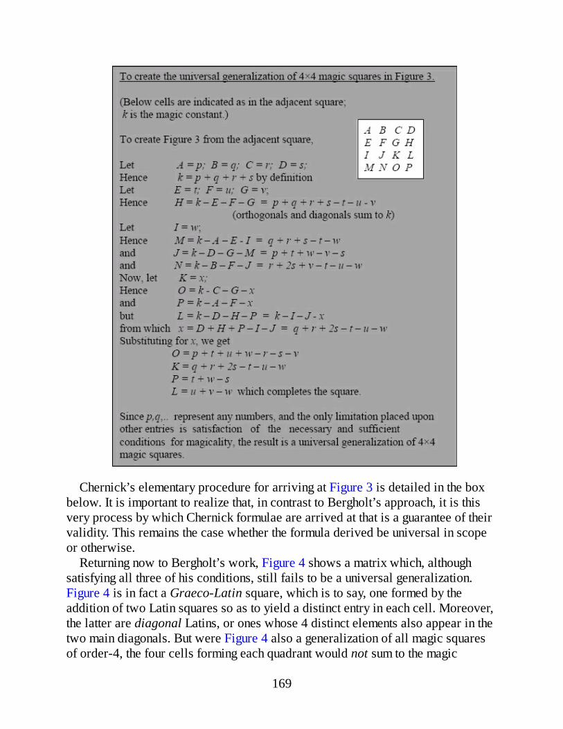
Chernick’s elementary procedure for arriving at Figure 3 is detailed in the boxbelow. It is important to realize that, in contrast to Bergholt’s approach, it is thisvery process by which Chernick formulae are arrived at that is a guarantee of theirvalidity. This remains the case whether the formula derived be universal in scopeor otherwise.

Returning now to Bergholt’s work, Figure 4 shows a matrix which, althoughsatisfying all three of his conditions, still fails to be a universal generalization.Figure 4 is in fact a Graeco-Latin square, which is to say, one formed by theaddition of two Latin squares so as to yield a distinct entry in each cell. Moreover,the latter are diagonal Latins, or ones whose 4 distinct elements also appear in thetwo main diagonals. But were Figure 4 also a generalization of all magic squaresof order-4, the four cells forming each quadrant would not sum to the magic

169

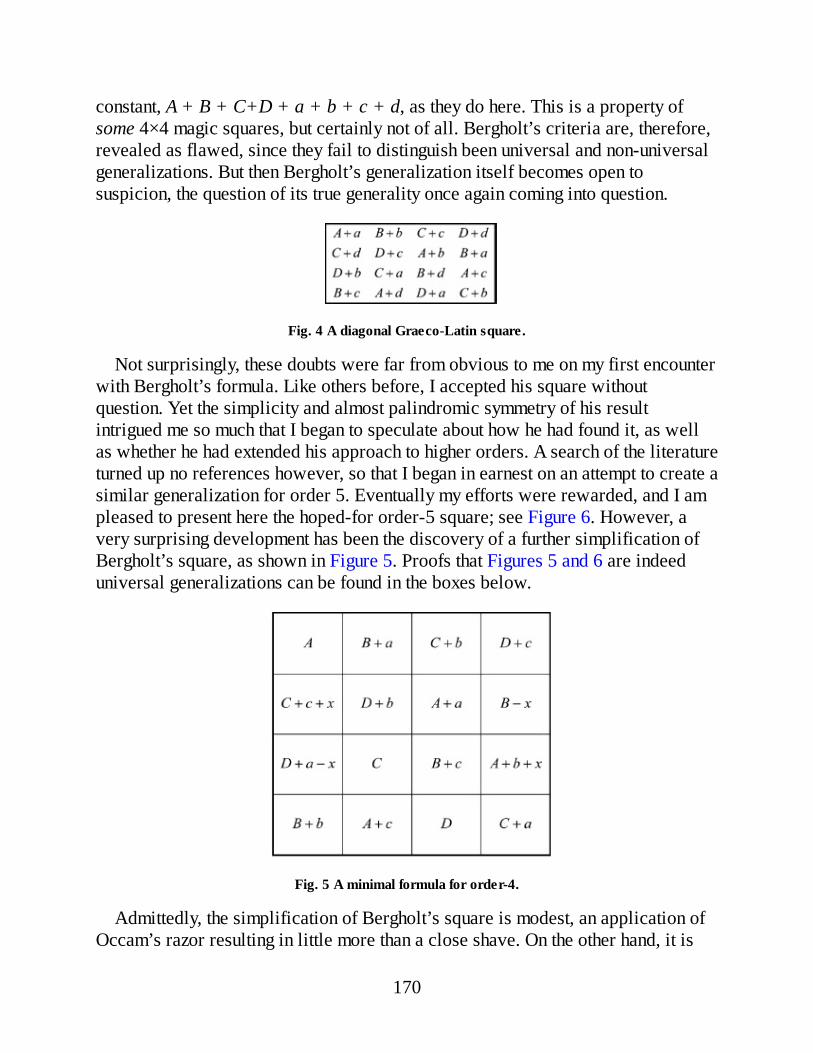
constant, A + B + C+D + a + b + c + d, as they do here. This is a property ofsome 4×4 magic squares, but certainly not of all. Bergholt’s criteria are, therefore,revealed as flawed, since they fail to distinguish been universal and non-universalgeneralizations. But then Bergholt’s generalization itself becomes open tosuspicion, the question of its true generality once again coming into question.

Fig. 4 A diagonal Graeco-Latin square.

Not surprisingly, these doubts were far from obvious to me on my first encounterwith Bergholt’s formula. Like others before, I accepted his square withoutquestion. Yet the simplicity and almost palindromic symmetry of his resultintrigued me so much that I began to speculate about how he had found it, as wellas whether he had extended his approach to higher orders. A search of the literatureturned up no references however, so that I began in earnest on an attempt to create asimilar generalization for order 5. Eventually my efforts were rewarded, and I ampleased to present here the hoped-for order-5 square; see Figure 6. However, avery surprising development has been the discovery of a further simplification ofBergholt’s square, as shown in Figure 5. Proofs that Figures 5 and 6 are indeeduniversal generalizations can be found in the boxes below.

Fig. 5 A minimal formula for order-4.

Admittedly, the simplification of Bergholt’s square is modest, an application ofOccam’s razor resulting in little more than a close shave. On the other hand, it is

170

easy to see that the eight variables occurring in any order-4 formula must eachappear at least four times: one for each row/column when the variable appears inthe magic constant; twice positive and twice negative when not. The minimumnumber of variable appearances is thus 8 × 4 = 32, as in Figure 5, for which reasonwe may call this a minimal formula.

Fig. 6

Figure 6 is in fact not a minimal formula, the very first example of which beingdue (to the best of my knowledge) to Prof. Don Knuth, with whom I correspondedon this topic. Later, a puzzle based on the problem of distinguishing universal from

171

non-universal formulae appeared under our names in the Journal of RecreationalMathematics1. Knuth’s minimal formula which featured in the puzzle presentationis shown in Figure 7.

The foundation of Bergholt’s approach rests in the observation that a numericaldiagonal Latin square is simultaneously a trivial type of magic square in whichonly n of the n2 entries are distinct; whereas a literal diagonal Latin square (i.e.,one using letters) can be interpreted as an algebraic generalization of such trivialsquares. He then had the ingenious idea of introducing modifications to the literalLatin square in a way that would preserve its magic properties while ensuring thateach cell becomes occupied by a distinct entry. This is effected by the arrangementof lower-case letters in his matrix. Similarly, both of my own generalizationsabove are elaborations upon Graeco-Latin squares. But Bergholt was still upagainst the problem of deciding whether a matrix so produced is a generalization ofall 4×4 magic squares or not. For there is no guarantee that the relationsestablished among the cells are not restrictive beyond the point dictated by thedefinition of a magic square. Having grasped his principle, it was not difficult todream up candidate squares for order-5, but the question remained of how theywere to be tested. The solution to this problem is of course pivotal in identifyinggenuinely universal formulae from among likely contenders.

Fig. 7

Following a lot of thought, eventually I came to see that if Chernick’sgeneralization was by definition universal (see first box above), any alternativeformula could only be a re-expression of that same generalization in different form.The test of a putative formula, in short, stood or fell by a demonstration of itsisomorphism with the Chernick-type square. Two of the above boxes providedemonstrations of isomorphism between Figures 5 and 6 and their correspondingChernick equivalents. It is ironic and fitting that Chernick held the key to Bergholt’svindication all along: for Bergholt’s formula is indeed a “completely generalformula” as may easily be verified in the same way as shown for Figure 5.

172

Reducing Formulae to Essentials

The formulae looked at above have all been generalizations of traditional oradditive magic squares, which is to say, those in which the sums of the numbers inevery row, column, and diagonal are alike. Analogous formulae for multiplicaitivesquares, showing constant products, can equally be created. On refelection,however, we see that, all other things being equal, the only change required in anysuch matrix would be the replacement of × for +, and 1/a for –a; where a may beany variable. This realization quite naturally expands to the unspecified binaryoperation,~, and the concept of a generalization of “~-itive” magic squares, similarin other respects to additive types, save that ~ replaces +, and the inverse a-1

replaces –a. Still further compression can be achieved by writing ab for a ~ b, anda for –a. These points find expression in Figure 8, a square that subsumes additiveand multiplicative magic squares in a single formula. By discarding redundantoperator signs, we not only increase the sweep of generalizations, but expose theessential structure with starker clarity.

Fig. 8 Another minimal formula for order-4.

This reduced form will be adopted in what follows, although in the discussion itwill be convenient to retain the familiar terminology of additive magic squares.Bear in mind though that justaposition (ab) will represent any binary operation, andā the inverse of a, so that the scope of variables is not restricted to numbers only,but embraces the elements of any abelian group. Figure 8, incidentally, is a secondexample of a minimal formula based on a diagonal Graeco-Latin square.

There is a further step that may be taken toward streamlining generalizations.Until now, the constant sum in each case has been represented by an expression thatis an accidental outcome of the matrix design. For instance, in the isomorphicsquares of Figures 3 and 5 it is p + q + r + s and A + B + C +D + a + b + c,respectively. To standardize this magic constant, all that is needed is to stipulate itsvalue at the outset, say k, and then to complete the generalization so as to complywith this new condition. In the Chernick square of Figure 3, for example, everyappearance of s would then be changed to k – (p + q + r). However, if the magicconstant is set to zero (or group identity element), k may be eliminated from the

173

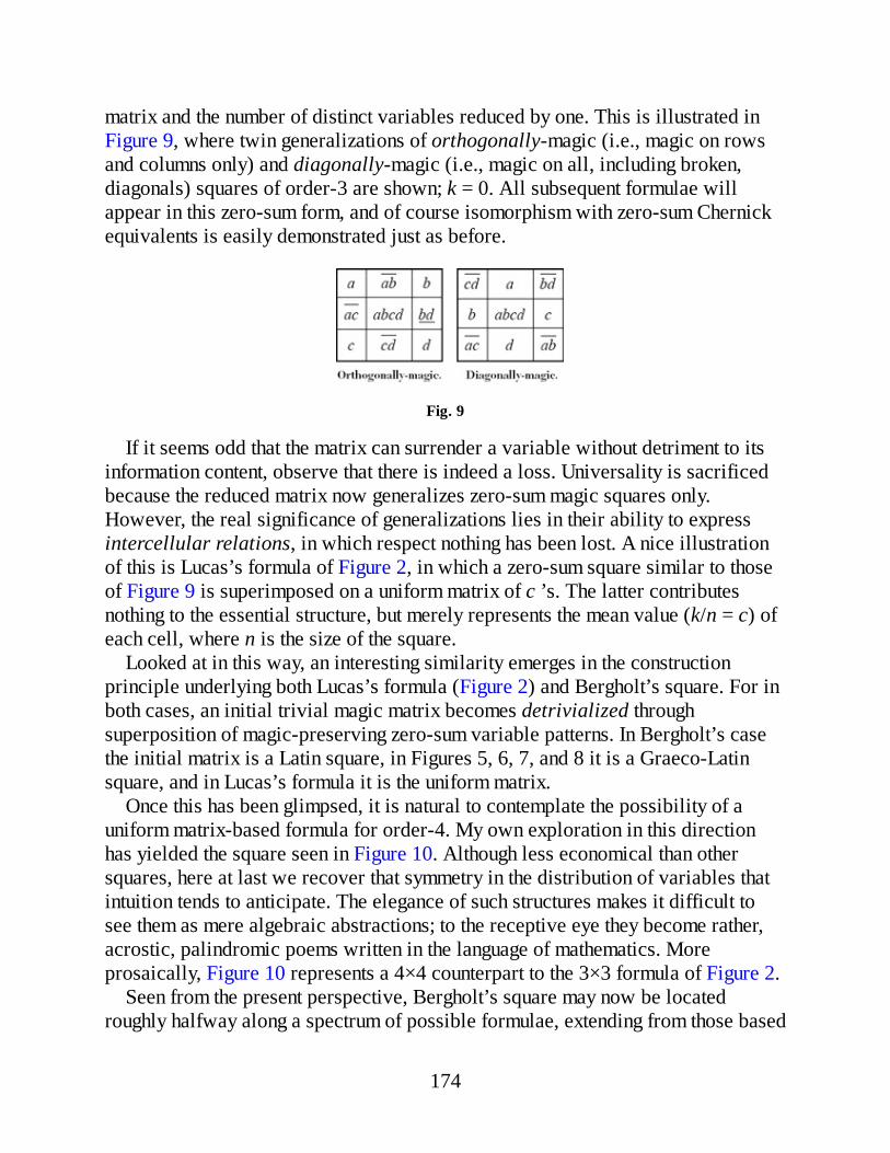
matrix and the number of distinct variables reduced by one. This is illustrated inFigure 9, where twin generalizations of orthogonally-magic (i.e., magic on rowsand columns only) and diagonally-magic (i.e., magic on all, including broken,diagonals) squares of order-3 are shown; k = 0. All subsequent formulae willappear in this zero-sum form, and of course isomorphism with zero-sum Chernickequivalents is easily demonstrated just as before.

Fig. 9

If it seems odd that the matrix can surrender a variable without detriment to itsinformation content, observe that there is indeed a loss. Universality is sacrificedbecause the reduced matrix now generalizes zero-sum magic squares only.However, the real significance of generalizations lies in their ability to expressintercellular relations, in which respect nothing has been lost. A nice illustrationof this is Lucas’s formula of Figure 2, in which a zero-sum square similar to thoseof Figure 9 is superimposed on a uniform matrix of c ’s. The latter contributesnothing to the essential structure, but merely represents the mean value (k/n = c) ofeach cell, where n is the size of the square.

Looked at in this way, an interesting similarity emerges in the constructionprinciple underlying both Lucas’s formula (Figure 2) and Bergholt’s square. For inboth cases, an initial trivial magic matrix becomes detrivialized throughsuperposition of magic-preserving zero-sum variable patterns. In Bergholt’s casethe initial matrix is a Latin square, in Figures 5, 6, 7, and 8 it is a Graeco-Latinsquare, and in Lucas’s formula it is the uniform matrix.

Once this has been glimpsed, it is natural to contemplate the possibility of auniform matrix-based formula for order-4. My own exploration in this directionhas yielded the square seen in Figure 10. Although less economical than othersquares, here at last we recover that symmetry in the distribution of variables thatintuition tends to anticipate. The elegance of such structures makes it difficult tosee them as mere algebraic abstractions; to the receptive eye they become rather,acrostic, palindromic poems written in the language of mathematics. Moreprosaically, Figure 10 represents a 4×4 counterpart to the 3×3 formula of Figure 2.

Seen from the present perspective, Bergholt’s square may now be locatedroughly halfway along a spectrum of possible formulae, extending from those based

174

on the uniform matrix, to those based on a Graeco-Latin square. Besides these,there are the Chernick-type squares, but of course all these different matrices aremathematicallly identical, being only alternative expressions of the sameunderlying algebriac form. Even so, the construction and classification of suchalgebraic squares opens as an attractive field of enquiry. Among the more obviousgoals of research is a uniform matrix-based version of order-5, while at the otherextreme there opens the possibility of 5×5 formula based upon three superimposedLatin squares. Incidentally, no 3×3 diagonal Latin square exists, but a Chernicksquare for this order is readily constructed.

Fig. 10

The concept of the magic square may of course be extended to matrices ofvarious shapes or dimension, and similarly, the cell entries together with theoperation(s) performed upon specific constellations of these in order to yield themagic constant need not be confined to familiar forms. In all such constructions thematrix functions as a purely mnemonic device for indicating a certain set ofequations. A study of the algebraic generalizations of such higher forms promisesto be rewarding, but, in conclusion, I turn rather in the opposite direction, towardthe use of these elementary algebraic techniques in elucidating a peculiar subset of4×4 squares.

Dudeney’s 12 Graphic Types

In the same year that witnessed the appearance of Bergholt’s square, H. E. Dudeneypublished an article including a classification of the 880 ‘normal’ or consecutive-integer magic squares of order 4. This was in The Queen, published on January15th, 1910. The same material was later incorporated into his book Amusements inMathematics. According to this scheme, every normal square belongs to one oftwelve “Graphic Types,” depending upon the distribution of its eight pairs of so-called complementary numbers, 1 and 16, 2 and 15, . . . , 8 and 9. Figure 11reproduces the twelve diagrams, where the lines indicate those cell couplesoccupied by complementary pairs. As a matter of fact, an identical categorization

175

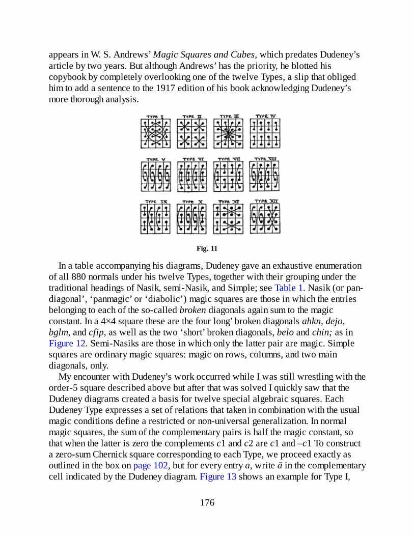
appears in W. S. Andrews’ Magic Squares and Cubes, which predates Dudeney’sarticle by two years. But although Andrews’ has the priority, he blotted hiscopybook by completely overlooking one of the twelve Types, a slip that obligedhim to add a sentence to the 1917 edition of his book acknowledging Dudeney’smore thorough analysis.

Fig. 11

In a table accompanying his diagrams, Dudeney gave an exhaustive enumerationof all 880 normals under his twelve Types, together with their grouping under thetraditional headings of Nasik, semi-Nasik, and Simple; see Table 1. Nasik (or pan-diagonal’, ‘panmagic’ or ‘diabolic’) magic squares are those in which the entriesbelonging to each of the so-called broken diagonals again sum to the magicconstant. In a 4×4 square these are the four long’ broken diagonals ahkn, dejo,bglm, and cfip, as well as the two ‘short’ broken diagonals, belo and chin; as inFigure 12. Semi-Nasiks are those in which only the latter pair are magic. Simplesquares are ordinary magic squares: magic on rows, columns, and two maindiagonals, only.

My encounter with Dudeney’s work occurred while I was still wrestling with theorder-5 square described above but after that was solved I quickly saw that theDudeney diagrams created a basis for twelve special algebraic squares. EachDudeney Type expresses a set of relations that taken in combination with the usualmagic conditions define a restricted or non-universal generalization. In normalmagic squares, the sum of the complementary pairs is half the magic constant, sothat when the latter is zero the complements c1 and c2 are c1 and –c1 To constructa zero-sum Chernick square corresponding to each Type, we proceed exactly asoutlined in the box on page 102, but for every entry a, write ā in the complementarycell indicated by the Dudeney diagram. Figure 13 shows an example for Type I,

176

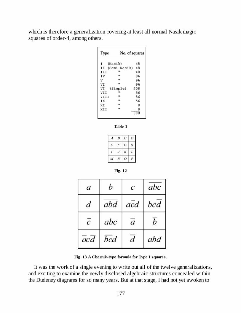
which is therefore a generalization covering at least all normal Nasik magicsquares of order-4, among others.

Table 1

Fig. 12

Fig. 13 A Chernik-type formula for Type I squares.

It was the work of a single evening to write out all of the twelve generalizations,and exciting to examine the newly disclosed algebraic structures concealed withinthe Dudeney diagrams for so many years. But at that stage, I had not yet awoken to

177

the advantages of zero-sum notation, with the result that arbitrary magic constantsrendered meaningful comparison of different squares impossible. Besides, thesematrices suffered from the redundancy and imperspicuity common to the Chernicktype, so that revision into reduced form became the obvious next step. This turnedout to be a formidable task. The Chernick squares play the part of Ariadne s thread,but trial-and-error guided by experience and intuition remains the only method ofadvance. Every square is capable of expression in a more or less unlimited varietyof forms, so that each underwent several stages of refinement before reachingcompletion. Finally, in order to maximize comparability of squares, carefulconsideration had to be given to the allocation of letter symbols. In Figure 14 canbe seen the “fruit of pensive nights and laborious days.” Here, it will be found, lieanswers to some of the intriguing questions concerning those 880 squares firstbrought to light by the labours of Frénicle de Bessy in 1693.

Reading the Runes

In the same way that certain properties common to every 4×4 magic square can beread off from a universal formula, so it is with the twelve Dudeney Types. Here Iconfine myself to three main observations.

1 As already noted, not only are Type-I squares Nasik (as Dudeney was wellaware), the sum of the entries in any 2×2 block of cells is again equal to the magicconstant, or zero in this case. This applies equally when the square is viewed astoroidally-connected, which is to say, when the top and bottom rows, as well asthe left-and right-hand columns are treated as adjacent to each other. Counting up,we find 16 of these zero-totalling 2×2 blocks, corresponding to the letters in Figure12 as follows: abef, bcfg, cdgh, adeh, efij, fgjk, ghkl, ehil, ijmn, jkno, klop, ilmp,abmn, bcno, cdop, admp. Magic squares that exhibit this property are said to becompact. Hence, among other things, the message contained in Figure 14 (I) is thatevery Type-I square (i.e., every normal square whose complementary pairs aredistributed as shown) is both Nasik and compact. However, we can go somewhatfurther than this.

178

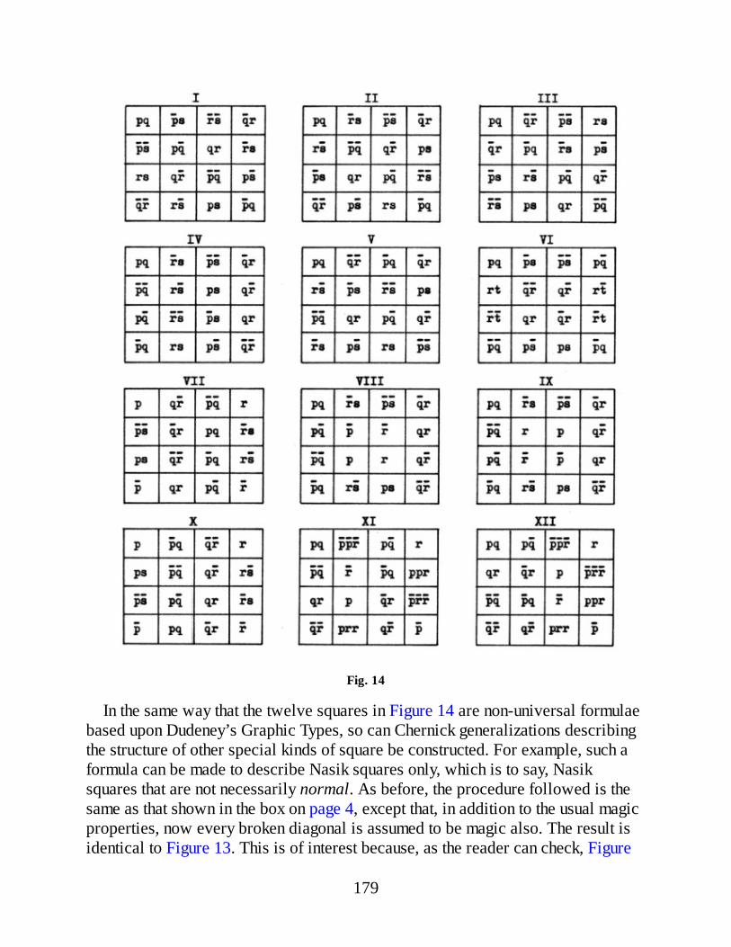
Fig. 14

In the same way that the twelve squares in Figure 14 are non-universal formulaebased upon Dudeney’s Graphic Types, so can Chernick generalizations describingthe structure of other special kinds of square be constructed. For example, such aformula can be made to describe Nasik squares only, which is to say, Nasiksquares that are not necessarily normal. As before, the procedure followed is thesame as that shown in the box on page 4, except that, in addition to the usual magicproperties, now every broken diagonal is assumed to be magic also. The result isidentical to Figure 13. This is of interest because, as the reader can check, Figure

179

13 turns out to be isomorphic with the Type-I formula of Figure 14. But this showsus that every 4×4 Nasik square, normal or otherwise, is always comprised of 8complementary pairs of entries, and is always compact, a finding that canalternatively be validated by constructing a Chernick generalization of all 4×4compact magic squares. The result is again identical to Figure 13, which againshows that the three characterizations, Type I, Nasik, and compact, define exactlythe same entity.

2 It will not have escaped readers that the set of 16 algebraic terms appearing inthe twelve formulae are in several cases the same. As already pointed out, “carefulconsideration had to be given to the allocation of letter symbols.” Specifically, thetwelve squares fall into four classes sharing identical cell entries:

Class 1 : Types I, II, III, I V, V, (and that subset of Type-VI when t = s or -s)Class 2 : Type VI (excluding the above subset members)Class 3 : Types VII, VIII, IX, XClass 4 : Types XI, XII

Clearly, the entries of a magic square belonging to a given Class may always betransposed to form a new square of different Type in the same Class. Hence, theentries in a Type-XI square, say, can always be rearranged to yield a Type-XIIsquare, and vice versa, while the entries in a Type-V square, for example, canalways be rearranged so as to form a Nasik, or Type-I square, and vice versa. Thisis no trivial finding, since it draws together and explains the entire family of allsuch magic rearrangements, as has never before been possible. Moreover, itobviates the necessity of having to prove any particular case, such as that found in[6], for example, in which the author devotes two pages to proving that Type-Isquares are always transposable into Type III, and vice versa. Figure 14 subsumesall such demonstrations, and more besides, in a single diagram.

Closer examination of the 16 algebraic terms comprising Class 1 reveal them asthe entries of an addition table, such as that in Figure 15 left. This is of interestbecause the entries in Lucas’s 3×3 formula of Figure 2 also belong to an additiontable (Figure 15 right), a fact that finds explanation in the Parallelogram Theoremthat is introduced in The Lost Theorem, here reproduced in Appendix V.

Less obvious is that the entries of Types XI and XII are really that special caseof Class 1 when s = pr. Class 4 magic squares are thus always transposable intoClass 1 Types, so that the entries in a Type-XI or XII square can also be rearrangedto yield a Type-I, or Nasik square, say.

3Dudeney’s table in Figure 11 shows that some normal squares of Type-VI aresemi-Nasik (96) and some Simple (208). But if now in Figure 14 (VI) we look atthe special cases when t = s, or t = –s, respectively, the resulting matrix becomes

180

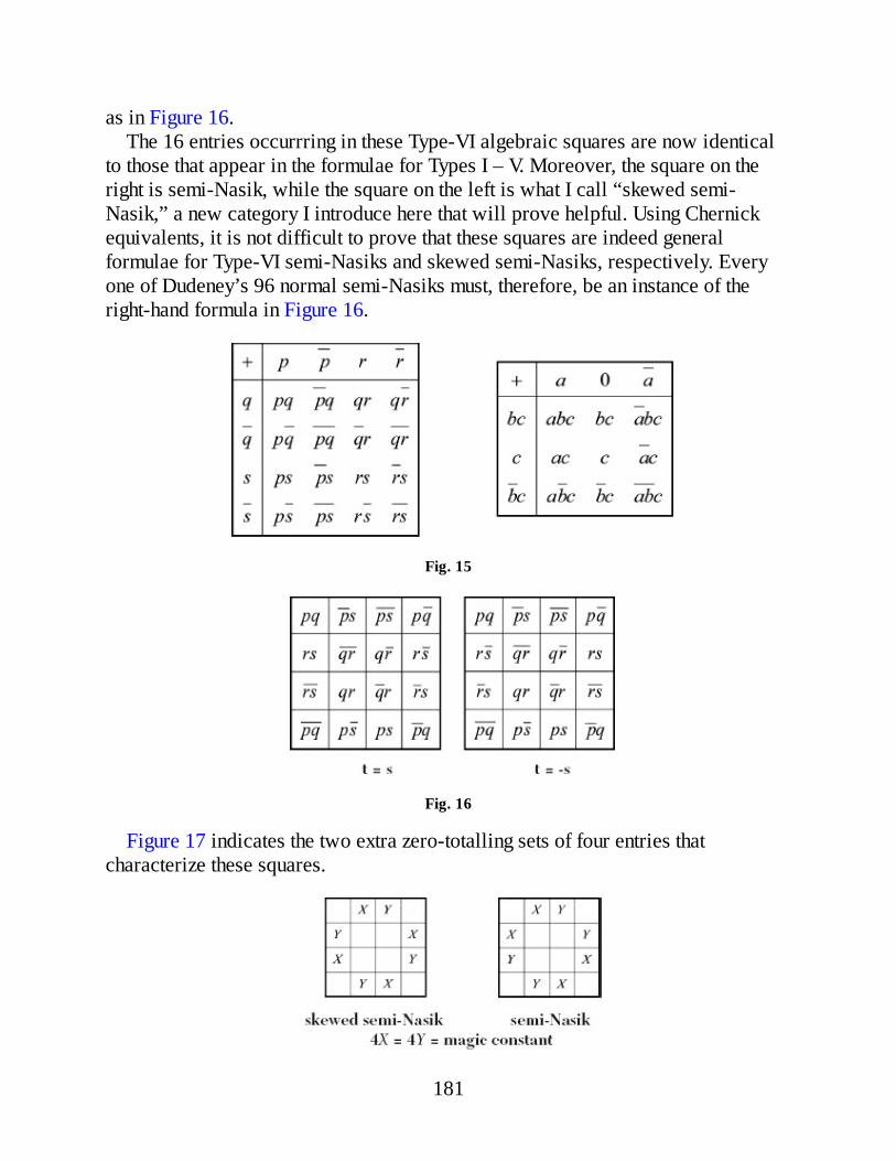
as in Figure 16.The 16 entries occurrring in these Type-VI algebraic squares are now identical

to those that appear in the formulae for Types I – V. Moreover, the square on theright is semi-Nasik, while the square on the left is what I call “skewed semi-Nasik,” a new category I introduce here that will prove helpful. Using Chernickequivalents, it is not difficult to prove that these squares are indeed generalformulae for Type-VI semi-Nasiks and skewed semi-Nasiks, respectively. Everyone of Dudeney’s 96 normal semi-Nasiks must, therefore, be an instance of theright-hand formula in Figure 16.

Fig. 15

Fig. 16

Figure 17 indicates the two extra zero-totalling sets of four entries thatcharacterize these squares.

181

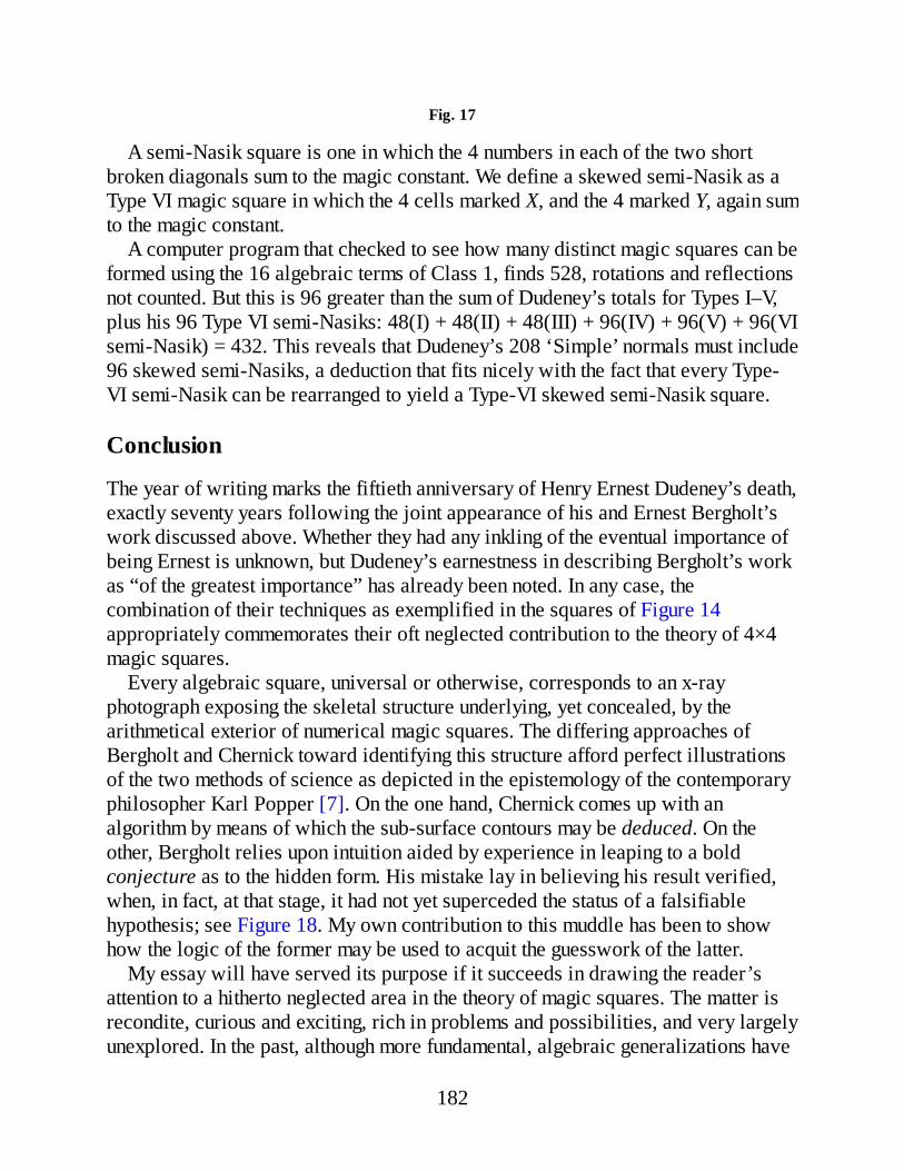
Fig. 17

A semi-Nasik square is one in which the 4 numbers in each of the two shortbroken diagonals sum to the magic constant. We define a skewed semi-Nasik as aType VI magic square in which the 4 cells marked X, and the 4 marked Y, again sumto the magic constant.

A computer program that checked to see how many distinct magic squares can beformed using the 16 algebraic terms of Class 1, finds 528, rotations and reflectionsnot counted. But this is 96 greater than the sum of Dudeney’s totals for Types I–V,plus his 96 Type VI semi-Nasiks: 48(I) + 48(II) + 48(III) + 96(IV) + 96(V) + 96(VIsemi-Nasik) = 432. This reveals that Dudeney’s 208 ‘Simple’ normals must include96 skewed semi-Nasiks, a deduction that fits nicely with the fact that every Type-VI semi-Nasik can be rearranged to yield a Type-VI skewed semi-Nasik square.

Conclusion

The year of writing marks the fiftieth anniversary of Henry Ernest Dudeney’s death,exactly seventy years following the joint appearance of his and Ernest Bergholt’swork discussed above. Whether they had any inkling of the eventual importance ofbeing Ernest is unknown, but Dudeney’s earnestness in describing Bergholt’s workas “of the greatest importance” has already been noted. In any case, thecombination of their techniques as exemplified in the squares of Figure 14appropriately commemorates their oft neglected contribution to the theory of 4×4magic squares.

Every algebraic square, universal or otherwise, corresponds to an x-rayphotograph exposing the skeletal structure underlying, yet concealed, by thearithmetical exterior of numerical magic squares. The differing approaches ofBergholt and Chernick toward identifying this structure afford perfect illustrationsof the two methods of science as depicted in the epistemology of the contemporaryphilosopher Karl Popper [7]. On the one hand, Chernick comes up with analgorithm by means of which the sub-surface contours may be deduced. On theother, Bergholt relies upon intuition aided by experience in leaping to a boldconjecture as to the hidden form. His mistake lay in believing his result verified,when, in fact, at that stage, it had not yet superceded the status of a falsifiablehypothesis; see Figure 18. My own contribution to this muddle has been to showhow the logic of the former may be used to acquit the guesswork of the latter.

My essay will have served its purpose if it succeeds in drawing the reader’sattention to a hitherto neglected area in the theory of magic squares. The matter isrecondite, curious and exciting, rich in problems and possibilities, and very largelyunexplored. In the past, although more fundamental, algebraic generalizations have

182

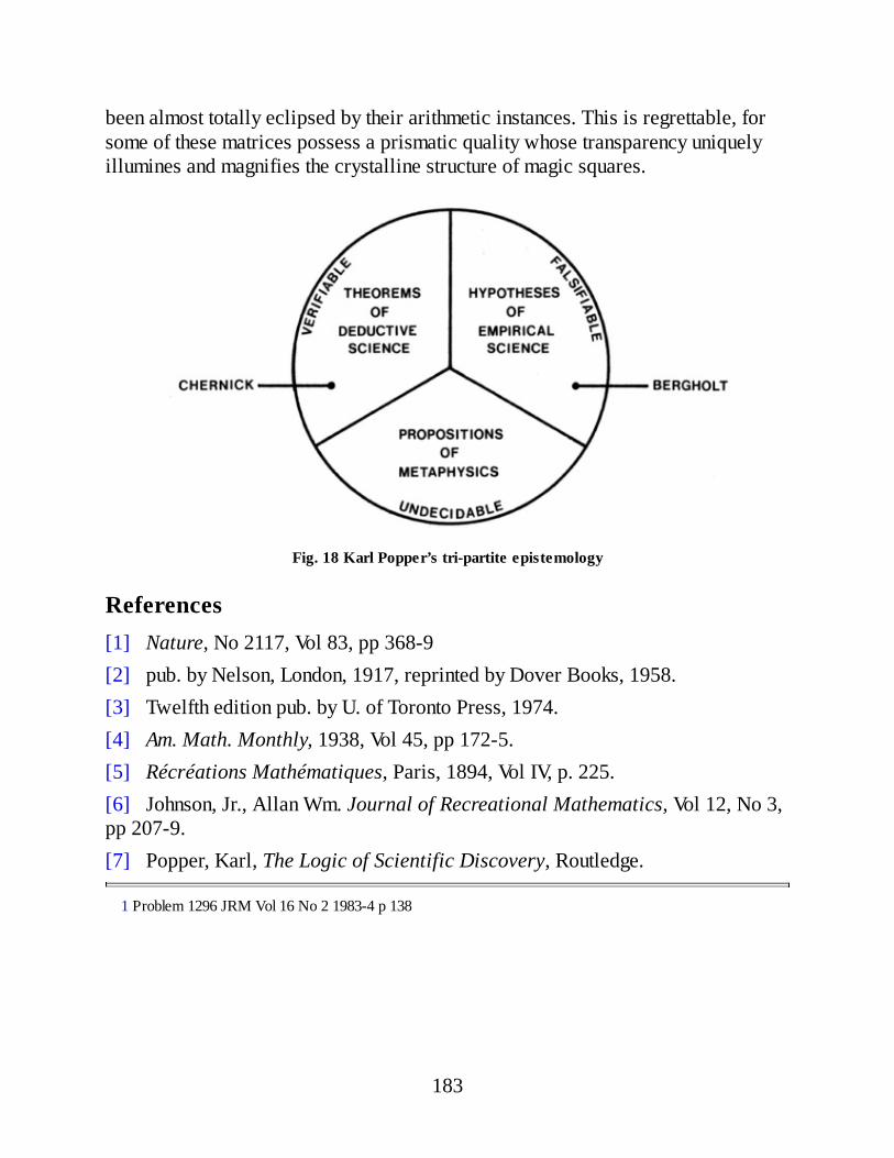
been almost totally eclipsed by their arithmetic instances. This is regrettable, forsome of these matrices possess a prismatic quality whose transparency uniquelyillumines and magnifies the crystalline structure of magic squares.

Fig. 18 Karl Popper’s tri-partite epistemology

References[1] Nature, No 2117, Vol 83, pp 368-9[2] pub. by Nelson, London, 1917, reprinted by Dover Books, 1958.[3] Twelfth edition pub. by U. of Toronto Press, 1974.[4] Am. Math. Monthly, 1938, Vol 45, pp 172-5.[5] Récréations Mathématiques, Paris, 1894, Vol IV, p. 225.[6] Johnson, Jr., Allan Wm. Journal of Recreational Mathematics, Vol 12, No 3,pp 207-9.[7] Popper, Karl, The Logic of Scientific Discovery, Routledge.

1 Problem 1296 JRM Vol 16 No 2 1983-4 p 138

183

Appendix III

New Advances with 4×4 Magic Squares

Introductory Note

The article to follow, New Advances with 4×4 Magic Squares presents the resultsof two strands of research carried out at various periods during the 1990s. Thiswork has never before appeared in print, nor indeed ever been submitted forpublication, although in recent years Harvey Heinz was kind enough to make itavailable on his excellent website: http://www.magic-squares.net. To the best ofmy knowledge, the matter of fertility here examined has never previously beenexplored. It would be nice to think that some of the intriguing questions thrown upby the findings here recorded will stimulate others to pursue these matters moredeeply. In my own view, the most obvious goal of future research would be todiscover a non-brute-force algorithm whereby the fertility of a set of 16 randomlychosen integers can be determined immediately, without need of a computer.

New Advances with 4×4 Magic Squares

Introduction

One of the best known results in the magic square canon is Bernard Frénicle deBessy’s enumeration of the 880 ‘normal’ 4×4 squares that can be formed using thearithmetic progression 1, 2 , . . . , 16. A natural question this suggests concernsnon-normal squares: Is 880 the largest total attainable if any 16 distinct numbersare allowed?

The answer is no. A computer program that will generate every squareconstructable from any given set of integers has identified 1,040 distinct squaresusing the almost arithmetic progression: 1, 2, 3, 4, 5, 6, 7, 8, 10, 11, 12, 13, 14, 15,16, 17. Note the doubled step from 8 to 10. The constant row-sum now becomes36. Extensive trials with alternative sets make it virtually certain that 1,040 is themaximum attainable (or 8 × 1,040 = 8,320, if rotations and reflections areincluded), although an analytic proof of this assumption is lacking. A listing of the1,040 squares can be had on request via email at lee.sal@inter.nl.net.

But if 1,040 is the maximum, what of lower totals? Can a set of numbers be

184

found that will yield any desired total under 1,040? If not, what totals are possible?In the absence of mathematical insight, trial-and-error was the only way to find out.The results of computer trials on thousands of different sets of small integers arepresented below. Again, although proof is lacking, there exist empirical groundsfor supposing that every possible total has been identified. Conceivably, one ortwo may have escaped the net. In any case, the wealth of new data represented bythese findings ought to provide a starting point for further researches in the field foryears to come. Some preliminary comments will be helpful in understanding theseresults.

Fertility and Set Structure

We define the fertility, f, of a set of 16 distinct elements, usually integers, as thetotal number of 4×4 magic squares it can produce, rotations and reflectionsincluded, divided by 32. This is because there are magic-preservingrearrangements besides rotations and reflections that are applicable to any squaresuch that it always has 31 variants that we may count as equivalent. For example,the two transformations shown in Figure 1 can be combined with rotations andreflections to produce all 32 squares.

Fig. 1

Thus, for the above-mentioned set, f = 8,320÷32 = 260, the putative maximum,while for a set of 16 consecutive integers, f = 880 × 8 ÷ 32 = 220. Besides thesetwo cases, integer sets exhibiting around one hundred different fertility values havebeen found, as listed in Tables 1 and 3.

Curiously, among these new finds is a second set yielding f = 220, but not usingconsecutive integers. In other words, for every one of the 880 normal squares,there exists a unique counterpart square using 16 numbers that do not form anarithmetic progression. An example is shown in Figure 2. The constant row sum isnow 38.

185

Fig. 2

It is interesting to note that whereas 4 distinct numbers adding to 34 can bechosen from {1, 2, . . . , 16} in 86 different ways, there are but 76 ways to choose4 numbers adding to 38 from the above set. Still more surprising is the outcome forthe set yielding 1,040 squares: 4 numbers adding to 36 can be chosen in just 80ways. The relation between the number of available magic 4-partitions and thenumber of squares produced would thus seem to be a lot looser than might havebeen supposed.

In comparing different sets it is useful to look at their structure rather than thenumbers occurring. This is because the fertility of a set is unaffected by adding aconstant to each member, or by multiplying each member by a constant, so thatdifferent numbers need not imply different fertilities. Sets are thus better describedby the sequence of 15 differences reduced to lowest terms occurring betweenadjacent members when ordered by magnitude. And since differences in the setsconsidered here are always less than ten, a single digit suffices for each. Thus, thetwo sets:

and

are both counted as particular instances of the structure: 111111121111111, whichis our canonical representation of all sets for which f = 260. The two set structuresyielding f = 220 are then 111111111111111, representing arithmetic series, and111211111112111, as exampled in the magic square of Figure 2.

The foregoing were all examples of palindromic or symmetric sets, which arethose composed of 8 conjugate pairs of numbers having equal sums, such as 1 + 16,2 + 15, . . . 8 + 9 in normal squares. If we think of the numbers as points along thereal number line, then conjugate pairs are points equidistant about a commoncentre, which is half their sum. Asymmetric sets are non-palindromic, but since thefertility of a set is unchanged by multiplying each member by –1, the fertility of anasymmetric set is the same as that of a set of same structure but reversed in order.

These remarks are sufficient to explain Table 1, which lists 66 asymmetric setsyielding fertility values in the range 1 to 71. No asymmetric set with a fertilityoutside this range was discovered; the five gaps indicate cases for which no

186

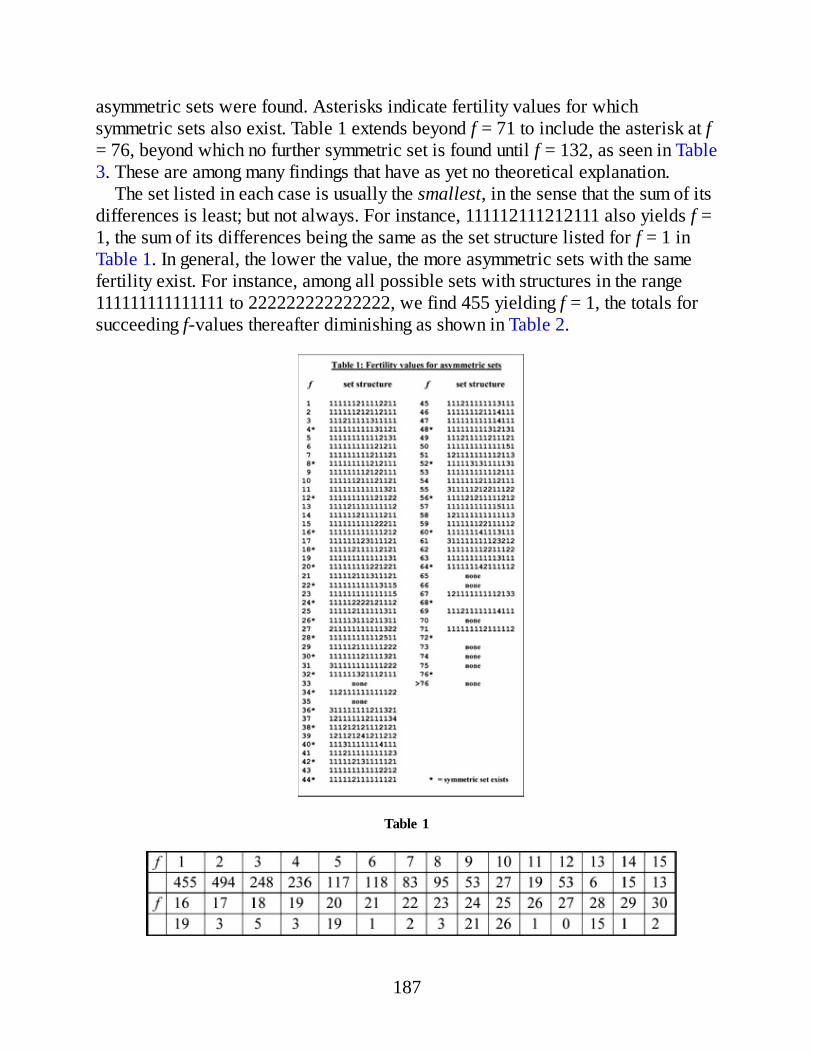
asymmetric sets were found. Asterisks indicate fertility values for whichsymmetric sets also exist. Table 1 extends beyond f = 71 to include the asterisk at f= 76, beyond which no further symmetric set is found until f = 132, as seen in Table3. These are among many findings that have as yet no theoretical explanation.

The set listed in each case is usually the smallest, in the sense that the sum of itsdifferences is least; but not always. For instance, 111112111212111 also yields f =1, the sum of its differences being the same as the set structure listed for f = 1 inTable 1. In general, the lower the value, the more asymmetric sets with the samefertility exist. For instance, among all possible sets with structures in the range111111111111111 to 222222222222222, we find 455 yielding f = 1, the totals forsucceeding f-values thereafter diminishing as shown in Table 2.

Table 1

187

Table 2

Fig. 3

This is not difficult to understand. Figure 3 shows a general formula thatdescribes the structure of every 4×4 magic square:

The number of magic squares that can be formed using the 16 algebraic terms inthe formula is clearly the same as the number of magic-preserving rearrangementsapplicable to any numerical magic square, and no more: 32. The fertility of thisalgebraic set is thus 1, but sets of greater fertility must represent particularinstances of the above, satisfying still more stringent conditions, and to that extentwill be scarcer. Hence the tapering off in totals as fertilities increase.

Turning now to Table 3, we find a total of 63 symmetric set structures, all ofthem yielding even fertility values in the range 4 to 260. No set with an odd-valuedfertility was found. Why is it that the fertility of symmetric sets is always even?

A tempting answer might seem to lie in the fact that symmetric squares come incomplementary pairs, such as the two shown in Figure 4.

Fig. 4

Switch the conjugate number pairs in one square to get the other, its so-calledcomplement. The trouble is that in this example the complement of each square isthe same thing as its rotation by 180 degrees. But this means that if one square isamong those in a set of f distinct specimens, then its complement (i.e., its rotation)will not be, so that this attempt to answer the original question fails. However, aproof that the fertility of symmetric sets is always even is derivable, although toospace-consuming to be included here.

Returning to Table 3, note that sets having fertilities in the range 1 to 76 havebeen found, with about 10 gaps, those appearing in the right hand column all beingmultiples of 4. Beyond these there is a wide gap up to 132, followed by most evenvalues from 132 to 220, again with about 10 gaps. No sets with 220 < f < 260 havebeen found. Both sets for f = 220 are recorded in the list.

188

The criteria used in selecting the particular set structure shown for each fertilityvalue in the Tables differs from case to case. Frequently, there exist manyalternative structures with the same fertility that could have been shown instead.Many of the results are due to Saleem al-Ashhab, a Jordanian email correspondent.Saleem was excited by my 1,040 squares find, and soon had his PC running nightand day in search of sets with new f values. In such cases I received only hisresults, but without details of the search procedure used. Still other results are dueto programs of my own, one of which checked blocks of sets in systematic order,counting the number of squares produced by each in turn and recording any newvalues found. I might mention that, thanks to insights due to Saleem, the fertility of achosen set of 16 integers took the final version of our computer program less than 2seconds to compute on a Pentium II machine. In another approach, sets composedof 16 random integers were generated one after the other, their fertility determinedand the result stored. Haphazard as this may seem, following an initial flood, withthe passage of time the number of fresh fertility values found slowed to a dribbleand then finally dried up completely, even following whole days of running time.Hence my confidence in the probable completeness of the results here presented. Itis worth mentioning that trials on sets using non-integral numbers produced nofertility values different to those recorded here.

189

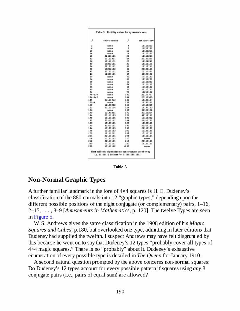
Table 3

Non-Normal Graphic Types

A further familiar landmark in the lore of 4×4 squares is H. E. Dudeney’sclassification of the 880 normals into 12 “graphic types,” depending upon thedifferent possible positions of the eight conjugate (or complementary) pairs, 1–16,2–15, . . . , 8–9 [Amusements in Mathematics, p. 120]. The twelve Types are seenin Figure 5.

W. S. Andrews gives the same classification in the 1908 edition of his MagicSquares and Cubes, p.180, but overlooked one type, admitting in later editions thatDudeney had supplied the twelfth. I suspect Andrews may have felt disgruntled bythis because he went on to say that Dudeney’s 12 types “probably cover all types of4×4 magic squares.” There is no “probably” about it. Dudeney’s exhaustiveenumeration of every possible type is detailed in The Queen for January 1910.

A second natural question prompted by the above concerns non-normal squares:Do Dudeney’s 12 types account for every possible pattern if squares using any 8conjugate pairs (i.e., pairs of equal sum) are allowed?

190

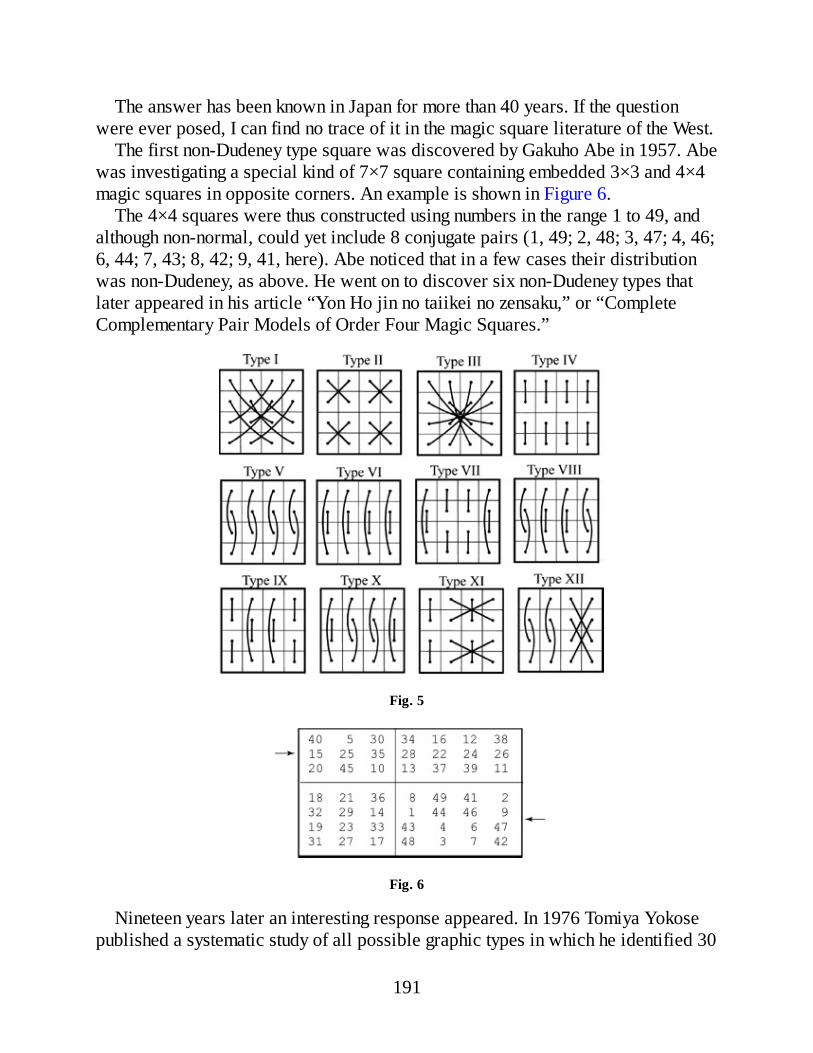
The answer has been known in Japan for more than 40 years. If the questionwere ever posed, I can find no trace of it in the magic square literature of the West.

The first non-Dudeney type square was discovered by Gakuho Abe in 1957. Abewas investigating a special kind of 7×7 square containing embedded 3×3 and 4×4magic squares in opposite corners. An example is shown in Figure 6.

The 4×4 squares were thus constructed using numbers in the range 1 to 49, andalthough non-normal, could yet include 8 conjugate pairs (1, 49; 2, 48; 3, 47; 4, 46;6, 44; 7, 43; 8, 42; 9, 41, here). Abe noticed that in a few cases their distributionwas non-Dudeney, as above. He went on to discover six non-Dudeney types thatlater appeared in his article “Yon Ho jin no taiikei no zensaku,” or “CompleteComplementary Pair Models of Order Four Magic Squares.”

Fig. 5

Fig. 6

Nineteen years later an interesting response appeared. In 1976 Tomiya Yokosepublished a systematic study of all possible graphic types in which he identified 30

191

in all, Dudeney’s 12 included [Sugei no pazuru (= “Mathematical Puzzles”), No.92,Sept-Oct., Showa 51, pp 17-25]. In my humble opinion Yokose’s work is amilestone in the development of the theory of 4×4 squares. As before, however,news of it seems never to have reached the West.

I am in debt to Nyr Indictor of New York State, and Guido de Mey of Brusselsfor translations of Abe’s and Yokose’s articles.

Still later I looked afresh at this question and, with a lot of help from MichaelSchweitzer, discovered four types that Yokose had missed. A computer search wasemployed; it would be tedious to describe the method here. Following on fromDudeney’s 12, I numbered the new types 13 to 34, as seen in Figure 7.

The ordering of Types 13 – 34 is partially random, partially systematic. It can beshown that whatever numbers appear in a Type-13 square, they can always berearranged so as to yield a Type-14 square, and vice versa. The same is true forany four Types appearing in the same horizontal row in the above diagram.Specifically, Types occupying the 2nd, 3rd and 4th columns can be derived from thatin the 1st column by means of the transforms T1, T2, and T1×T2, respectively,shown at the beginning of this article.

Fig. 7

192

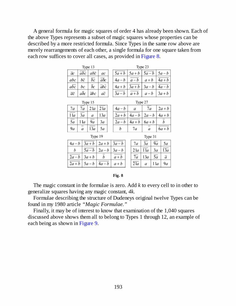
A general formula for magic squares of order 4 has already been shown. Each ofthe above Types represents a subset of magic squares whose properties can bedescribed by a more restricted formula. Since Types in the same row above aremerely rearrangements of each other, a single formula for one square taken fromeach row suffices to cover all cases, as provided in Figure 8.

Fig. 8

The magic constant in the formulae is zero. Add k to every cell to in other togeneralize squares having any magic constant, 4k.

Formulae describing the structure of Dudeneys original twelve Types can befound in my 1980 article “Magic Formulae.”

Finally, it may be of interest to know that examination of the 1,040 squaresdiscussed above shows them all to belong to Types 1 through 12, an example ofeach being as shown in Figure 9.

193

Fig. 9

194

Appendix IV

The Dual of the Lo shu

Introductory Note

A couple of blows have already been aimed at the iconic reputation of the Lo shumagic square in the course of Concluding Remarks. In The Dual of the Lo shuwhich started life as the first part of a longer, unfinished article on ambimagicsquares, I seek to deliver the coup de grâce. The Lo shu, it emerges, is not theunicorn we have always taken it to be, but merely one half of a pantomime horse.Ah, but is it the back half or the front? In any case, it will be no use locking thestable door after the horse has bolted it. Because a horse that bolts doors can onlybe a pantomime horse, which is what I set out to prove. The essay, not previouslypublished, was written in 1999.

The Dual of the Lo shu

“Various .. authors .. have asserted that the earliest magic square known[outside China] was given by Theon of Smyrna, a Neo-Pythagorean, about 130A.D. However, if they had looked up this so-called ‘magic square’ of Theon’s,they would have seen that it was not a magic square in any sense of the term.”

Schuyler Cammann [1]

“This array of numbers [Theon’s square] has therefore not the slightest thing todo with magic squares and deserves no place in the history of magic squares.”

W. Ahrens [2] [author’s translation]

Duality Denied

Cammann and Ahrens, the two authors quoted above, ought to know what they aretalking about. The first has written several oft-cited monographs on ancientChinese magic squares, while the second is the author of a celebrated German twovolume classic of recreational mathematics, Mathematische Unterhaltungen UndSpiele. So what exactly is this thing, ‘Theon’s square’, against which they areunited in their contempt?

195

Imagine a text on Taoist philosophy that expounds the Yin principle but withoutmentioning the Yang. Or an abridgment of Lewis Caroll’s Through the LookingGlass that introduces Tweedledee yet omits any reference to Tweedledum. Anunlikely scenario perhaps, and yet something equivalent to it is exactly the state ofaffairs in the realm of 3×3 magic squares.

“The literature on magic squares is vast,” wrote Martin Gardner. Anexaggeration perhaps, but as I have said myself in The Lost Theorem, innumerablebooks and articles on magic squares begin with a discussion of 3×3 types, theproperties of which have long been regarded as completely understood [3]. And inalmost all of those books and articles will be found the oldest and most famousmagic square of all. It is the 3×3 square of Chinese origin known as the Lo shu, aprototype so revered among aficionados that it enjoys the status of an iconicemblem; see Figure 1. The weird thing about all these writings on the Lo shu,however, lies in what they don’t say. I refer to the total absence of any mention ofthe Lo shu’s twin or duplicate square, or as we should say in mathematicallanguage, its dual.

Fig. 1 The Lo shu.

I can imagine that this reference to the dual of the Lo shu, innocuous enough tothe lay reader, will be greeted with incredulity on the part of more seasonedstudents, none of whom will have heard of it for exactly the reason just outlined.That is, to the best of my knowledge, there exists not a single reference to theexistence of this dual anywhere in the ‘vast’ literature on magic squares. On thecontrary, there are even experts on the subject who will deny the contingencyoutright. I have already quoted two of them. They are our two learned savants,Cammann and Ahrens, the authors for whom Theon’s square is such a pain in theneck. So what (to return to our starting point) is this object, Theon’s square?

Theon’s Square

The definition of a magic square means that it occupies a halfway house betweenorthomagic squares and panmagic squares. In the former, sometimes calledsimple, or semimagic squares, the diagonal requirement is dropped, with the therows and columns, or orthogonals alone needing to show equal sums. In the latter,also known as panmagic, pandiagonal or Nasik squares, the totals in every

196

diagonal, including the so-called ‘broken’ diagonals, are the same as those in all ofthe orthogonals. In Figure 2, the broken diagonals are occupied by afh, cdh, ibd,and gbf.

Fig. 2

In fact, although panmagic squares exist for all higher orders, a 3×3 panmagicsquare using nine distinct numbers is impossible to construct.

Broken diagonals can however be mended by bringing together the top andbottom edges of the square to make a cylinder which is then stretched and bentsmoothly in a circle until its ends meet to form a closed tube or torus. In a squarearray of 3×3 thus ‘toroidally connected,’ the left and right hand edges coincide, asdo those at top and bottom, with the result that every diagonal, like everyorthogonal, becomes a closed loop of 3 cells. The eight immediate neighbors ofeach cell are then the same as if the square were surrounded with copies of itself,as in using it as a tile to cover the plane. The closed loops are then reflected inrepeated cycles of 3 elements along horizontal, vertical, and inclined paths as seenin Figure 3.

Fig. 3

This same wallpaper pattern can be viewed as if built up from repeated copiesof any of its constituent 3×3 areas, of which there are nine, each corresponding toone of the nine possible permutations of the 3 rows and/or 3 columns. All nine areshown in Figure 4.

197

Fig. 4

Figure 2 is thus one among nine squares that are indistinguishable when viewedas toroidally connected. That is, there are nine different ways in which the toruscan be cut along two axes perpendicular to each other, unfolded, and then flattenedinto a square. Or in other words, any particular 3×3 square is but one among ninealternative planar projections of the torus it represents.

Viewed thus, any idea of broken diagonals as the poor cousins in the familydisappears, and we discover a simple parity between orthogonals and diagonals,the relations among the 3 rows and 3 columns finding matching counterparts in therelations among the 3 ‘\’– diagonals, or slopes and 3 ‘/’– diagonals or slants. Notehowever, that the same does not hold of even-order arrays such as 4×4, in whichrows and columns intersect on one cell, while slopes (a) and slants (b) mayintersect on two; see Figure 5.

Fig. 5

A notable consequence of this symmetry in the case of 3×3 arrays is thatorthogonal elements can be switched with diagonal elements to create a twin ordual of the original square as shown in Figure 6.

Fig. 6

198

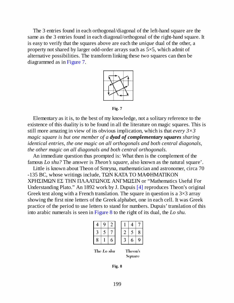
The 3 entries found in each orthogonal/diagonal of the left-hand square are thesame as the 3 entries found in each diagonal/orthogonal of the right-hand square. Itis easy to verify that the squares above are each the unique dual of the other, aproperty not shared by larger odd-order arrays such as 5×5, which admit ofalternative possibilities. The transform linking these two squares can then bediagrammed as in Figure 7.

Fig. 7

Elementary as it is, to the best of my knowledge, not a solitary reference to theexistence of this duality is to be found in all the literature on magic squares. This isstill more amazing in view of its obvious implication, which is that every 3×3magic square is but one member of a dyad of complementary squares sharingidentical entries, the one magic on all orthogonals and both central diagonals,the other magic on all diagonals and both central orthogonals.

An immediate question thus prompted is: What then is the complement of thefamous Lo shu? The answer is Theon’s square, also known as the natural square’.

Little is known about Theon of Smryna, mathematician and astronomer, circa 70-135 BC, whose writings include, TΩN KATA TO MAΦHMATIKONXPHΣIMΩN EΣ THN ΠΛAATΩNOΣ ANΓMΩΣIN or “Mathematics Useful ForUnderstanding Plato.” An 1892 work by J. Dupuis [4] reproduces Theon’s originalGreek text along with a French translation. The square in question is a 3×3 arrayshowing the first nine letters of the Greek alphabet, one in each cell. It was Greekpractice of the period to use letters to stand for numbers. Dupuis’ translation of thisinto arabic numerals is seen in Figure 8 to the right of its dual, the Lo shu.

Fig. 8

199

It is the square refered to in the opening quotations. Cammann and Ahrens, theauthors cited, were of course right to dismiss claims that Theon’s square is a magicsquare. But the fact that there were people who asserted it was, or who saw in it afirst attempt at a magic square makes it all the stranger that nobody seems ever tohave noticed that all six diagonals, as well as both central orthogonals, sum to 15.Least of all, Theon himself, I suspect, who probably knew nothing of magicsquares, and who introduces his diagram as a purely didactic device in discussing5 as the arithmetic mean of pairs summing to 10, the latter a number that loomslarge in Pythagorean philosophy. In any case, the two statements made aboutTheon’s square, that it is “not a magic square in any sense of the term” and that ithas “not the slightest thing to do with magic squares and deserves no place in thehistory of magic squares” betrays a lack of understanding on the part of these twosupposed experts in the field that is simply breathtaking.

Admittedly, from the point of view of the magic square connoisseur, twoblemishes mar Theon’s square. First, a single glance is enough to grasp its pattern.The serial order of the numbers in the columns makes for a transparent structurethat lacks all mystique, and hence charm, and without which it attracts scantinterest. Second, unlike the Lo shu, in which every straight line of numbers adds to15, no equivalent elegance is enjoyed by the same-sum triads in Theon’s square.However, both blemishes disappear when the two squares are compared astoroids, on the surface of which diagonals are no more broken than orthogonals.The dual of a 3×3 magic square is thus not another magic square, but a square ofequivalent magic.’

There exists a considerable literature devoted to the Lo shu, much of it infectedwith the kind of crypto-mystic twaddle met with in Feng Shui. It would be nice tothink that once news of the dual gets out things will change. The discovery that ‘the’Lo shu is only one-half of a double act is surely going to come as quite arevelation. But of course such a big change will take time to absorb. So themessage should be kept simple. How about: “Hey guys, snap out of it: it’s not alone shu, it is a pair of shus.”

References[1] Shuyler Cammann, The Evolution of Magic Squares in China, Journal of the

American Oriental Society. LXXX, 1960, pp 116-124.[2] W. Ahrens, Studien über die magischen Quadrate der Araber, Der Islam, VII,

1917, pp 186-250.[3] L. Sallows, The Lost Theorem, The Mathematical Intelligencer, 1997, 19; 4,

pp 51-4

200

[4] J. Dupuis, Theon de Smyrne, Libraire Hachette et Cie, Paris 1892, pp.167-8.

201

Appendix V

The Lost Theorem

Introductory Note

It seems that open season has been declared on the Lo shu, because here again inThe Lost Theorem, I am to be found bemoaning a blemish in its structure. “Whydon’t you leave that wretched square alone?” I can hear my critics say. But mymotive is of course merely practical, for it is only through identifying flaws inexisting magic squares that we can hope to produce improved specimens. And themore revered the square in question, then the more searching must be our criticalexamination. The ‘atomic’ square here described is a pearl born of the grit at itsheart–a particle of grit that is the Lo shu itself. Had it not been for defects in thelatter, a path to the former might never have been found. The essay appeared in TheMathematical Intelligencer in 1997. I am also indebted to Christian Boyer, whohas been kind enough to include it on his scholarly and extremely impressivewebsite http://www.multimage.com/indexengl.htm.

The Lost Theorem

“Almost the last word has been said on this subject”—H. E. Dudeney on magic squares [1]

A magic square, as all the world knows, is a square array of numbers whose sum inany row, column, or main diagonal is the same. So-called “normal” squares areones in which the numbers used are 1,2,3, and so on, but other numbers may beused. Squares using repeated entries are deemed trivial. We say that a square ofsize N × N is of order-N. Clearly, magic squares of order-1 lack glamour, while amoment’s thought shows that a square of order-2 cannot be realized using distinctentries. The smallest magic squares of any interest are thus of order-3.

Writing in Quantum recently [2], Martin Gardner offered $100 to anyone able toproduce a 3×3 magic square composed of any nine distinct square numbers. So farnobody has produced a solution, or proof of its impossibility, although a near missI discovered is seen in Figure 1, a specimen whose rows, columns, and just one ofthe two main diagonals sum to the same number, itself a square: 1,472. It was

202

while tinkering in connection with this problem that I was startled to discover anelementary correspondence between 3×3 magic squares and parallelograms. Thereason for my surprise is worth explaining.

Fig. 1

Magic squares have been a special hobby of mine for over twenty years; theliterature on the topic, much of which I have collected, is extensive. As alreadynoted, 3×3 magic squares are the smallest and, hence, simplest types, for whichreason they are the earliest to appear in history, as well as being the mostthoroughly investigated squares of all. Innumerable books and articles on magicsquares begin with a discussion of 3×3 types, the properties of which have longbeen regarded as completely understood. Writing in the well known MathematicalRecreations published in 1930, for instance, Maurice Kraitchik begins by sayingthat, “The theory of the squares of the third order is simple and complete . . .”, andthen goes on to present that theory in just two pages of text.

Yet for all its extreme simplicity, the elementary correspondence withparallelograms that I had stumbled upon while working on Gardner’s problem, has,to the best of my knowledge, never previously been identified. I feel sure that manyreaders will share my incredulity on inspecting the theorem below. They may agreewith me that the correlation with parallelograms it describes is so basic that itdeserves to be regarded as the fundamental theorem of order-3 magic squares, andthe very first thing that any newcomer to the subject should learn. How then couldsuch a theorem escape the attention of every researcher in the field from ancienttimes down to the present day?

An explanation lies in the orthodox focus on magic squares using naturalnumbers. Once our attention broadens to include squares that use complex numbers,the familiar integer types become only a special case, preoccupation with whichhas obscured the wider picture. Moving beyond this narrow view, we step into arealm of greater clarity and harmony. And at the very center of that realm, we shallfind an undiscovered prize, the atomic magic square.

Standard Theory

What makes a 3×3 square magic?Figure 2 shows the well-known algebraic formula due to Édouard Lucas that

describes the structure of every magic square of order 3:

203

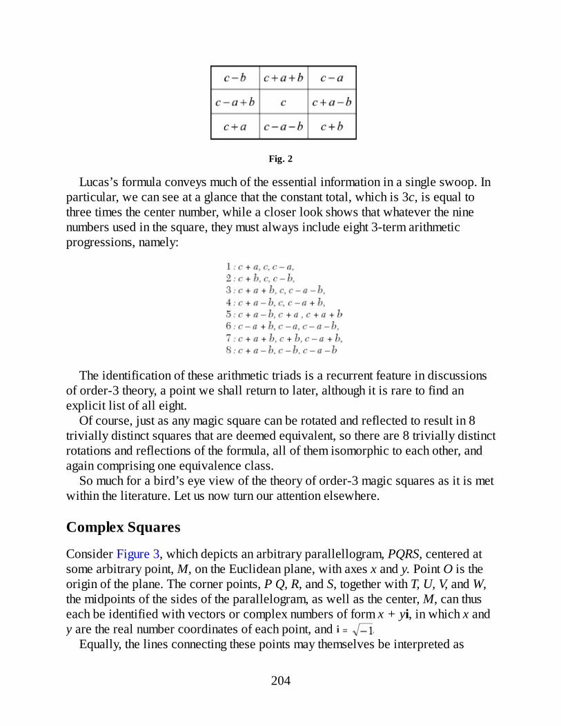
Fig. 2

Lucas’s formula conveys much of the essential information in a single swoop. Inparticular, we can see at a glance that the constant total, which is 3c, is equal tothree times the center number, while a closer look shows that whatever the ninenumbers used in the square, they must always include eight 3-term arithmeticprogressions, namely:

The identification of these arithmetic triads is a recurrent feature in discussionsof order-3 theory, a point we shall return to later, although it is rare to find anexplicit list of all eight.

Of course, just as any magic square can be rotated and reflected to result in 8trivially distinct squares that are deemed equivalent, so there are 8 trivially distinctrotations and reflections of the formula, all of them isomorphic to each other, andagain comprising one equivalence class.

So much for a bird’s eye view of the theory of order-3 magic squares as it is metwithin the literature. Let us now turn our attention elsewhere.

Complex Squares

Consider Figure 3, which depicts an arbitrary parallellogram, PQRS, centered atsome arbitrary point, M, on the Euclidean plane, with axes x and y. Point O is theorigin of the plane. The corner points, P Q, R, and S, together with T, U, V, and W,the midpoints of the sides of the parallelogram, as well as the center, M, can thuseach be identified with vectors or complex numbers of form x + yi, in which x andy are the real number coordinates of each point, and

Equally, the lines connecting these points may themselves be interpreted as

204

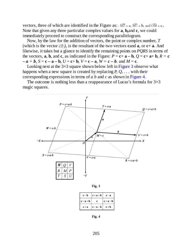
vectors, three of which are identified in the Figure as: .Note that given any three particular complex values for a, b,and c, we couldimmediately proceed to construct the corresponding parallelogram.

Now, by the law for the addition of vectors, the point or complex number, T(which is the vector ), is the resultant of the two vectors cand a, or c+ a. Andlikewise, it takes but a glance to identify the remaining points on PQRS in terms ofthe vectors, a, b, and c, as indicated in the Figure: P = c+ a – b, Q = c+ a+ b, R = c– a + b, S = c – a – b, U = c+ b, V = c – a, W = c – b. and M = c.

Looking next at the 3×3 square shown below left in Figure 3 observe whathappens when a new square is created by replacing P, Q, . . . with theircorresponding expressions in terms of a b and c as shown in Figure 4.

The outcome is nothing less than a reappearance of Lucas’s formula for 3×3magic squares.

Fig. 3

Fig. 4

205

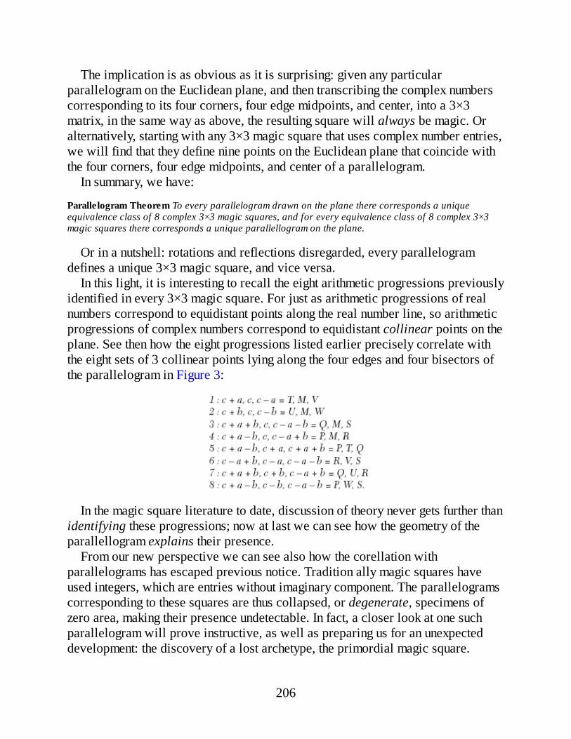
The implication is as obvious as it is surprising: given any particularparallelogram on the Euclidean plane, and then transcribing the complex numberscorresponding to its four corners, four edge midpoints, and center, into a 3×3matrix, in the same way as above, the resulting square will always be magic. Oralternatively, starting with any 3×3 magic square that uses complex number entries,we will find that they define nine points on the Euclidean plane that coincide withthe four corners, four edge midpoints, and center of a parallelogram.

In summary, we have:

Parallelogram Theorem To every parallelogram drawn on the plane there corresponds a uniqueequivalence class of 8 complex 3×3 magic squares, and for every equivalence class of 8 complex 3×3magic squares there corresponds a unique parallellogram on the plane.

Or in a nutshell: rotations and reflections disregarded, every parallelogramdefines a unique 3×3 magic square, and vice versa.

In this light, it is interesting to recall the eight arithmetic progressions previouslyidentified in every 3×3 magic square. For just as arithmetic progressions of realnumbers correspond to equidistant points along the real number line, so arithmeticprogressions of complex numbers correspond to equidistant collinear points on theplane. See then how the eight progressions listed earlier precisely correlate withthe eight sets of 3 collinear points lying along the four edges and four bisectors ofthe parallelogram in Figure 3:

In the magic square literature to date, discussion of theory never gets further thanidentifying these progressions; now at last we can see how the geometry of theparallellogram explains their presence.

From our new perspective we can see also how the corellation withparallelograms has escaped previous notice. Tradition ally magic squares haveused integers, which are entries without imaginary component. The parallelogramscorresponding to these squares are thus collapsed, or degenerate, specimens ofzero area, making their presence undetectable. In fact, a closer look at one suchparallelogram will prove instructive, as well as preparing us for an unexpecteddevelopment: the discovery of a lost archetype, the primordial magic square.

206

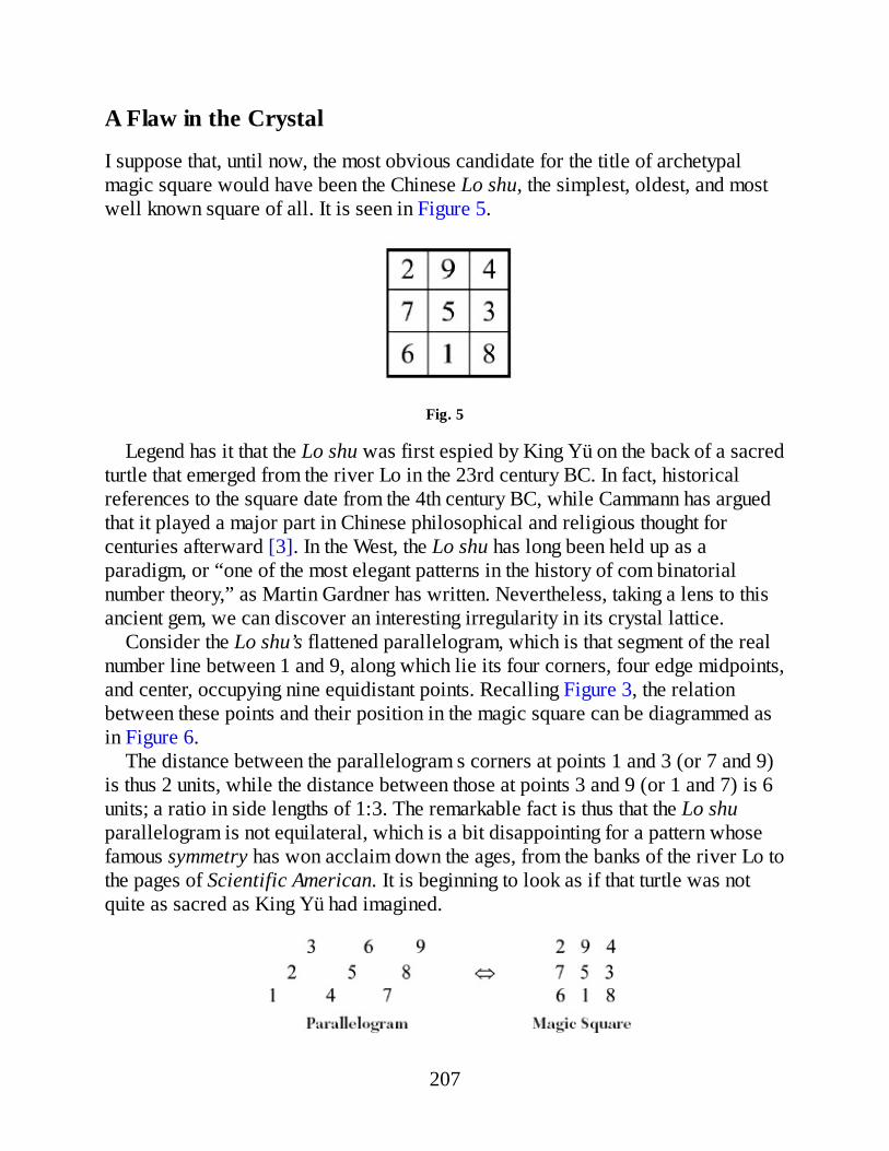
A Flaw in the Crystal

I suppose that, until now, the most obvious candidate for the title of archetypalmagic square would have been the Chinese Lo shu, the simplest, oldest, and mostwell known square of all. It is seen in Figure 5.

Fig. 5

Legend has it that the Lo shu was first espied by King Yü on the back of a sacredturtle that emerged from the river Lo in the 23rd century BC. In fact, historicalreferences to the square date from the 4th century BC, while Cammann has arguedthat it played a major part in Chinese philosophical and religious thought forcenturies afterward [3]. In the West, the Lo shu has long been held up as aparadigm, or “one of the most elegant patterns in the history of com binatorialnumber theory,” as Martin Gardner has written. Nevertheless, taking a lens to thisancient gem, we can discover an interesting irregularity in its crystal lattice.

Consider the Lo shu’s flattened parallelogram, which is that segment of the realnumber line between 1 and 9, along which lie its four corners, four edge midpoints,and center, occupying nine equidistant points. Recalling Figure 3, the relationbetween these points and their position in the magic square can be diagrammed asin Figure 6.

The distance between the parallelogram s corners at points 1 and 3 (or 7 and 9)is thus 2 units, while the distance between those at points 3 and 9 (or 1 and 7) is 6units; a ratio in side lengths of 1:3. The remarkable fact is thus that the Lo shuparallelogram is not equilateral, which is a bit disappointing for a pattern whosefamous symmetry has won acclaim down the ages, from the banks of the river Lo tothe pages of Scientific American. It is beginning to look as if that turtle was notquite as sacred as King Yü had imagined.

207

Fig. 6

Fig. 7

However, as a prisoner in Flatland, the Lo shu is doomed to this imbalance:squash any equilateral parallelogram, and two pairs of edge midpoints and twocorners will coincide, forcing repeated entries in the associated magic square. Inother words, unless it is trivial, an asymmetrical parallelogram must accompanyevery non-complex magic square, the one on the (mock?) turtle included.

Where then is the magic square with the symmetrical parallelogram that King Yüwas denied?

The Atomic Square

Of course, the most symmetrical case of all is an equilateral parallelogram that isequiangular as well: the square.

A magic square whose associated parallelogram is again a square; the idea is atonce compelling. But what kind of a magic square would that be? To find out, allwe have to do is draw a square on the plane, read off the complex values of its fourcorners, etc, and then write these into a 3×3 matrix in the usual way. Simplest of allis the canonical or atomic case seen in Figure 7.

It is a square centered on the origin of the plane, such that its four corners andfour edge midpoints coincide with the 8 complex integers immediately surrounding

208

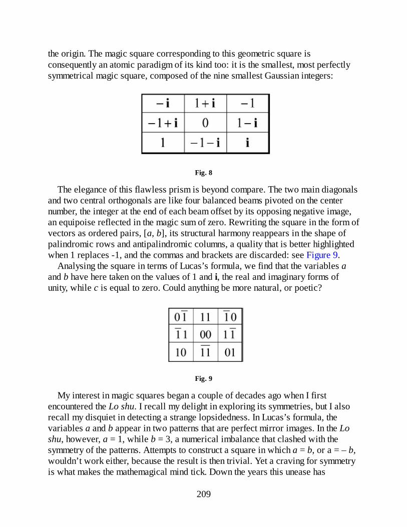
the origin. The magic square corresponding to this geometric square isconsequently an atomic paradigm of its kind too: it is the smallest, most perfectlysymmetrical magic square, composed of the nine smallest Gaussian integers:

Fig. 8

The elegance of this flawless prism is beyond compare. The two main diagonalsand two central orthogonals are like four balanced beams pivoted on the centernumber, the integer at the end of each beam offset by its opposing negative image,an equipoise reflected in the magic sum of zero. Rewriting the square in the form ofvectors as ordered pairs, [a, b], its structural harmony reappears in the shape ofpalindromic rows and antipalindromic columns, a quality that is better highlightedwhen 1 replaces -1, and the commas and brackets are discarded: see Figure 9.

Analysing the square in terms of Lucas’s formula, we find that the variables aand b have here taken on the values of 1 and i, the real and imaginary forms ofunity, while c is equal to zero. Could anything be more natural, or poetic?

Fig. 9

My interest in magic squares began a couple of decades ago when I firstencountered the Lo shu. I recall my delight in exploring its symmetries, but I alsorecall my disquiet in detecting a strange lopsidedness. In Lucas’s formula, thevariables a and b appear in two patterns that are perfect mirror images. In the Loshu, however, a = 1, while b = 3, a numerical imbalance that clashed with thesymmetry of the patterns. Attempts to construct a square in which a = b, or a = – b,wouldn’t work either, because the result is then trivial. Yet a craving for symmetryis what makes the mathemagical mind tick. Down the years this unease has

209

continued to quietly smoulder, until recent events brought the parallelogramtheorem to light, and, with it, a sudden resolution of the mystery in the shape of theatomic square, whose symmetry is without flaw. It is a relief; I look forward tosleeping at nights once again.

The above article first appeared in The Mathematical Intelligencer Vol 19, No. 4, pp 51-4, 1997. It isreprinted here with the kind permission of Springer Science + Business Media.

References[1] H.E. Dudeney, Amusement in Mathematics, p. 119.[2] M. Gardner, The Magic of 3×3, Quantum, January/February 1996, pp. 24-6.[3] S. Cammann, The Magic Square of Three in Old Chinese Philosophy and

Religion, History of Religions I (1961), pp. 37-80.

210

Glossary

alphamagic square A special kind of numerical magic square, the numbers ofwhich can be represented by their word equivalents (‘one,’ ‘two,’ etc.) so that thetotal number of letters then occurring in each row, column and diagonal, is thesame.

algebraic generalization An array in which algebraic terms consisting ofvariables and operators describe the necessary relations among numbers occupyingthe cells of a corresponding magic square.

almost-magic square A square in which every row and column, as well as just oneof the two main diagonals is magic.

ambimagic square A novel kind of magic square (due to the author) in which thesum of the numbers in every orthogonal (row and column) is the same, while theproduct of the numbers in every diagonal (including ‘broken’ diagonals) is alsoconstant. It can be shown that the magic sum in an ambimagic square of order-3 isnecessarily zero. The converse of an ambimagic square (constant orthogonalproducts, constant diagonal sums) is a ‘mabimagic’ square.

area square The numerical magic square that is formed by the piece areas in acorresponding 2-D square. Since differently shaped pieces may be of same area,area squares are frequently trivial.

bi-magic square In the realm of numerical magic squares a bi-magic specimen isone in which the squares of the numbers appearing also form a magic square. In thepresent account, the term has been borrowed to indicate a geomagic square inwhich the pieces are able to tile two distinct targets.

co-diagonal In any square, the diagonal running from top right to bottom left (/).

compact A (geo)magic square of 4×4 in which the four elements in each of itssixteen 2×2 sub-squares will combine to produce the constant total or target. Everynasik numagic square of order 4 is compact, and every compact numagic square oforder 4 is nasik. 2-D squares can however be nasik without being compact, orcompact without being nasik.

211

complementary pairs A numerical magic square of order N is composed of N2/2complementary pairs when the latter all sum to half the magic constant. Similarly, ageometrical magic square of order N is composed of N2/2 geometricallycomplementary pairs when the latter will combine to produce an identical shape.See geometric complement.

degenerate square A square containing repeated entries, also known as a trivialsquare.

demi-nasik A geomagic square in which, besides the two main diagonals, thereexist at least two non-parallel broken diagonals that are also magic (i.e., containtarget-tiling piece sets). See semi-nasik.

detrivialize In the case of algebraic squares, the process of adding variables so asto produce a unique expression in every cell. In the case of geometric squares, theprocess of appending/excising keys and keyholes so as to yield a distinctly shapedpiece in every cell.

dimension The dimension of a geomagic square is simply the same as that of thepieces of which it is comprised.

disconnected piece A compound piece consisting of two or more separatedislands considered as a single structure whose components are joined rigidly, ifinvisibly, to each other; also, a disjoint piece.

disjoint piece See disconnected piece.

disjoint arcs A particular case of a disconnected piece in which the separatedcomponents are all segments belonging to the same circular arc.

empty piece The invisible man among pieces. A piece consisting of an empty setof points.

Eulerian square A square formed by ‘superimposing’ two suitable Latin squaressuch that every cell becomes occupied by a distinct entry. Also known as aGraeco-Latin square.

diagonal Latin square A latin square in which the set of entries occupying each ofthe two main diagonals is the same as it is for each row and column.

212

Dudeney’s graphic types A classification of the 880 normal order-4 magicsquares into twelve distinct Types, according to the distribution of their constituentcomplementary pairs.

fertilityThe number of different magic squares that can be produced using a givenset of N2 distinct numbers.

five types of area square The five possible algebraic structures underlyingnumerical magic squares, whether containing repeated entries or not.

formula An alternative expression for an algebraic generalization.

geo-alphamagic square A cross-breed between a geomagic square that usespolyominoes and an alphamagic square. Distinct number-words adorn thepolyominopieces, a single letter appearing in each cell. The numbers are so chosenthat their sum is the same in every line, just as the piece shapes are chosen so as totile the target in every line.

geo-Eulerian Square A geometrical interpretation of a Graeco-Latin or Euleriansquare.

geomagic square A square array of N-dimensional figures that will combine inevery line so as to form an identical compound figure. See the formal definition inAppendix 1.

geometric complemen t A set of pieces is said to comprise so manycomplementary pairs when the two members of each pair will combine so as toform an identical shape. The piece pairs are then said to be the geometriccomplement of each other.

geometric variable On analogy with algebraic variables, a certain shape may beregarded as a ‘geometric variable’, in that it can be seen as standing for a range ofcontingent shapes.

geolatin square A Latin square of N×N using geometrical shapes as elements, andsuch that the N shapes in each line tile a common target. Alternatively, a trivialgeomagic square derived from a Latin template.

Graeco-Latin square See eulerian square.

213

graphic types See Dudeney’s graphic types.

isometric grid A regular grid like a rectangular grid that is seen on tiling the planewith unit equilateral triangles joined edge to edge.

key A shape that is appended to an existing piece

keyhole An indentation or region that is excised from an existing piece

Latin square An N×N array containing N distinct entries, each of them occurringexactly once in every row and column.

Lo shu A famous 3×3 magic square of early Chinese origin.

lug-type key A shape that is appended toa piece so as to form a distinctprojection, in contrast to the result of appending a size-altering key.

mabimagic square See ambimagic square.

magic line Short for a row, column, diagonal or other group of cells, the entries ofwhich will combine to produce the required constant outcome (add to required sumor tile required target).

main diagonal In any square, the diagonal running from top left to bottom right (\).

nasik A magic square in which every diagonal, including the so-called ‘broken’diagonals, is magic. Nasik squares are also known as panmagic, pandiagonal,diabolic and satanic.

normal square A numerical magic square of size N×N that uses the numbers 1, 2, .. . , N2. A 2-D geomagic square whose area square is a normal numagic square.

numagic square An abbreviation for ‘numerical magic square.’

order The size of a magic square. A square of size N×N is said to be of order-N.

orthogonals The rows and columns of a square.

pentomino A polyomino composed of five unit squares.

picture-preserving square A geomagic square in which the surface composition of

214

each target is the same.

polycube A three-dimensional shape formed of unit cubes that are joined face-to-face.

polyform A figure, shape, or structure composed of repeated atoms. The latter maybe of any dimension, provided all are the same.

polymagic square A geomagic square in which the pieces used are all polyforms.

polyomino A shape composed of unit squares joined edge -to-edge.

polyiamond A shape composed of unit equilateral triangles joined edge-to-edge.

polyhex A shape composed of unit regular hexagons joined edge-to-edge.

toroidally-connected A square regarded as if inscribed on a torus. That is, thesquare is imagined to be rolled into a cylinder which is then bent smoothly in acircle until its two ends meet. The top row thus becomes adjacent to the bottomrow, and the left-hand column adjacent to the right-hand column. What appear asbroken diagonals in the original square now become fully-fledged diagonals.

self-interlocking square A special kind of geomagic square using essentiallysquare pieces that can be made to coincide with the square-cell boundaries of thearray that contains them. The effect produced is spectacular. Thus far, the onlyknown specimens are of order-4. Whether or not there exist self-interlockingsquares of higher orders is unknown.

semimagic square A square in which only rows and columns are magic. Anorthogonally magic square.

semi-nasik A (geo)magic square in which, besides the two main diagonals, thereexist at least two parallel broken diagonals that are also magic (i.e., contain target-tiling piece sets). See demi-nasik.

size-alterning key A shape that can be appended to an existing piece so as toproduce an apparent enlargement or elongation of the piece, rather than thesuggestion of a distinct appendage.

substrate A trivial geomagic square showing repeated piece shapes that is used asa starting point for further elaboration into a non-trivial square.

215

target The common shape, region, or structure that is formed or tiled byassembling its component pieces that are found occupying every row, column, andmain diagonal in a geomagic square.

template An algebraic square that is used as a guide in constructing a geomagicsquare. In doing so, distinct variables are translated into distinct geometric shapes.Where variables occur in both positive and negative form, the former areinterpreted as shapes to be appended, the latter as shapes to be removed or cut out.

three-dimensional square A geomagic square using solid rather than planarpieces. In general, geomagic square may employ pieces of any dimension.

trivial square A square in which one or more entries occur more than once.

uniform array A square in which every entry is the same.

weakly-connected Pieces which are almost disconnected but in which somecomponent regions are not wholly separate but meet in a single point.

216

References

[1] S. Cammann, “Old Chinese magic squares,” Sinologica, 7(1962): 14-53.[2] S. Cammann, “The magic square of three in old Chinese philosophy and

religion,” History of Religions 1 (1961): 37-80.[3] L. Sallows, Alphamagic squares, in Richard Guy & Bob Woodrow, The

Lighter Side of Mathematics, (Math. Assoc. of America, 1994), pp. 305-339.[4] L. Sallows, “The Lost Theorem,” The Mathematical Intelligencer, 19:4

(1997): 51-54.[5] Édouard Lucas, Recreations Mathematiques, Vol. IV (1894): 225.[6] M. D. Hirschhorn The 1976 Summer School, Parabola, Vol 13 Issue 1 2-5,18;

Issue 2: “More Tessellations with Convex Equilateral Pentagons,” 20-2.[7] M. D. Hirschhorn; D. C. Hunt, “Equilateral convex pentagons which tile the

plane,” J. Combin. Theory Ser. A, 39 (1985): 1-18.[8] Martin Gardner, Time Travel and Other Mathematical Bewilderments, (San

Francisco: W.H. Freeman and Co., 1988), pp. 174-5.[9] Doris Schattschneider, In Praise of Amateurs, ed. David A. Klarner, (Prindle,

Weber, Schmidt 1981), pp. 140-66.[10] L. Sallows, “Geomagische vierkanten,” Pythagoras 1 (Sept. 2009): 12-15. L.

Sallows “Geomagische vierkanten met Lucas’ formule,” Pythagoras, 2 (Nov.2009). L. Sallows “Panmagisch versus most perfect,” Pythagoras 4 (Feb.2010). L. Sallows “4×4 Geomagisch vierkant met 8 complementaire paren,Pythagoras 1 (Sept. 2010).

[11] J. Dénes & A.D. Keedwell, Latin Squares and Their Applications, (EnglishUniversities Press, 1974).

[12] H.E. Dudeney, Amusements in Mathematics, (New York: Dover Publications,Inc.,1958).

[13] Barclay Rosser and R. J. Walker, “On the transformation group for diabolicmagic squares of order four,” Bulletin of the Mathematical Society Vol XLVI(June 1938): 416-20.

[14] L.S. and Penrose R., British Journal of Psychology 49 (1958): 31-3.[15] M. Coster, “Prijsvraag: wees een magiër,” Pythagoras 2 (Nov. 2009): 14-17.[16] M. Coster, “De magiërs zijn onder ons,” Pythagoras 6 (June 2010): 16-19.[17] Martin Gardner, “Mathematical Games,” Scientific American Vol 234 No 1

(Jan. 1976): 118-223.[18] Greg Ross, http://www.futilitycloset.com/index.php?s=lee+sallows[19] L. Sallows, “Nieuw archief voor wiskunde” Vijfde Serie deel 10, No 1(Maart

217

2009): 70.[20] Jack Chernick, “Solution of the general magic square,” American

Mathematical Monthly Vol 45 (1938): 172-5.[21] H.S. Hahn, “Another property of magic squares,” Fibonacci Quarterly 13

(Oct. 1975): pp 205-8.

218

www.doverpublications.com

219