geographical ranges in macroecology - ku
TRANSCRIPT
Geographical ranges in macroecology:Processes, patterns and implications
Thesis submitted for the degree of PhD in Biology
University of Copenhagen, 2010
Michael Krabbe Borregaard

D E P A R T M E N T O F B I O L O G Y F A C U L T Y O F S C I E N C E U N I V E R S I T Y O F C O P E N H A G E N
D E P A R T M E N T O F B I O L O G Y F A C U L T Y O F S C I E N C E U N I V E R S I T Y O F C O P E N H A G E N
Geographical ranges in macroecology:Patterns, processes and implications
PhD thesisMichael Krabbe Borregaard
May 2010
Supervised by
Prof. Dr. Carsten Rahbek

2

3
PrefaceThis thesis is the result of a three-year PhD project based at the Center for Macroecol-ogy, Evolution and Climate at the University of Copenhagen in Denmark. The project was supervised by Prof. Dr. Carsten Rahbek. In addition to my base in Copenhagen, the thesis work also included a three-month stay at the University of Vermont, USA, with Dr. Nicholas C. Gotelli. The PhD stipend was financed by a full Faculty of Sci-ence grant from the University of Copenhagen.
The present thesis consists of three parts: The first part is a short synopsis that gives an overview of the background for the thesis and summarizes the main find-ings. The second part consists of five chapters, including one book chapter, one major review paper, one technical forum paper, and two analytical papers. Three of these chapters are already published as scientific articles, and are included here in their published format. Finally, I have added two chapters, in which I have acted as a co-author, as appendices.
Michael Krabbe BorregaardCopenhagen, May 2010

4

5
ContentsAcknowledgements....................................................................... 7
Summary........................................................................................ 9
Resumé........................................................................................ 11
Synopsis....................................................................................... 13
Chapter.1:.................................................................................... 29Causality of the relationship between geographic distribution and species abundance
Chapter.2:.................................................................................... 55Are species-range distributions consistent with range-size heritability?
Chapter.3:.................................................................................... 75Dispersion fields, diversity fields and null models: uniting range sizes and species richness
Chapter.4:.................................................................................... 83Geographic species pools determine the richness-temperature relationship for South American birds
Chapter.5:.................................................................................... 99Spatial distribution
Appendix.I:................................................................................ 109Range size patterns in European freshwater trematodes
Appendix.II:............................................................................... 127From complex spatial dynamics to simple Markov chain models: do predators and prey leave footprints?

6
7
AcknowledgementsFirst and foremost, I would like to thank Carsten Rahbek for many enlightening dis-cussions and ping-pong of ideas over the years, and for working hard to create an in-spiring environment for macroecology at the University of Copenhagen. I wish him more time for the former and less time for the latter in coming years; for though he is a skilled administrator, he is an extraordinary scientist. I thank Nicholas Gotelli for hosting me in Vermont and taking the time to make my stay profitable, for inspiring me to learn to program a computer, and for teaching me about working efficiently – the latter, alas, I have had a tendency to forget again on many occasions. And, I would like to thank Gary Graves for sharing a very creative and inspiring work process with me, and for having a bit of sound advice on just about everything.
I want to thank all of my colleagues: notably Adser, Anders, Anne-Sofie, Bjørn, Christian, David, Elisabeth, Hans-Henrik, Irina, Jonas, Lisbeth, Peter and Susanne from the Center for Macroecology, for good friendship, inspiring discussions and a lot of fun over the years. I also feel thankful towards all the other great people at the Section for Ecology and Evolution for creating a pleasant work atmosphere. I thank Ditte for having the courage to venture with me into the mist of classic and Bayesian statistics, and Gösta for highly interesting discussions on models and maths, and for always being ready to chat or answer some arcane statistical question.
Big thanks go to Ted and Alexa Hart for taking us in when we went to Vermont; it meant a lot to meet their friendliness when our little family was far away from home. Thanks also go to Miguel Araujo and the people of the Biochange Lab, for hosting the always enjoyable lab retreats in Iberia.
Finally, I thank my wife, Katrine, for supporting me in trying to realize my dreams, and for having patience when that is necessary - which, alas, is not rarely.

8

9
SummaryThis thesis investigates how ecological patterns at large scale are shaped by the geo-graphic ranges of species. A species’ range is the geographic area in which an animal lives and breeds. The size of such ranges vary tremendously: some species only exist in a tiny area, whereas others, like humans, are distributed over the entire Earth.
Species’ ranges are one of the basic units of the science of macroecology, which deals with patterns in the distribution of life on Earth. An example of such patterns is the large geographic variation in species richness between areas. These patterns are closely linked to the ranges of individual species, in two distinct ways: Ecology and evolution determine the ranges of species; and at the same time the ranges of species shape ecological patterns. This link between geographical ranges and macroecologi-cal patterns is the subject of the present thesis. To investigate the link, I draw upon a wide range of approaches, including statistical comparative analysis, computer simu-lations and null models.
The core of the thesis is constituted by five independent scientific articles. These chapters fall naturally within two thematic groups:
The first group consists of articles that investigate how ecology and evolution de-termine species’ ranges. The central paper in this group is a large review article about one of the best described patterns in ecology: That species with large ranges tend to also be very locally abundant within their range. In the article I review the potential causes for this relationship. In going through the mechanisms, I distinguish between ‘structural’ causes, such as differences between the niches of species; and ‘dynamic’ causes, such as dispersal of individuals among populations. A central conclusion is that both of these types of mechanisms contribute to creating the relationship, al-though the causalities of the two types follow disparate pathways. A second paper addresses how the sizes of geographical ranges could be affected by evolution. Here I used a computer simulation to investigate the possibility that ranges are ‘inher-ited’ between species at speciation, constituting a species-level parallel of inheritance in individuals. Such inheritance is theoretically possible, though highly controver-sial. Nevertheless, a simulation model demonstrated that species-level heritability of range sizes is consistent with observed range-size distributions.
Finally, this thematic group includes a popularly written book chapter, where the causes and consequences of the spatial distribution of organisms are introduced more generally.
The second group consists of several papers investigating the link between ranges

10
and richness patterns. Variation in species richness is probably a result of geographi-cal variations in climatic conditions: humid and warm places are home to many more species and dry and cold areas. However, by investigating the coincidence of distribu-tions of different species, I demonstrate that the regional fauna of areas is determined by the configuration of biomes; and that the size of this regional fauna plays an im-portant role for creating patterns of species richness. A related approach to investi-gating the link between ranges and richness is to use so-called range-diversity plots, which are tools for describing covariance in species’ distributions. In the final paper, I consider the applicability of this approach, and define a set of null models for the interpretation of range-diversity plots.

11
ResuméDenne afhandling er en undersøgelse af hvordan økologiske mønstre på stor skala
påvirkes af arters geografiske udbredelser. En arts-udbredelse er et geografisk om-råde hvori en dyreart lever og yngler. Størrelsen af sådanne udbredelser kan variere enormt: nogle arter findes kun i et ganske lille område, mens andre arter, såsom men-nesket, er udbredte over hele jorden.
Arts-udbredelser er en af de grundlæggende enheder i videnskaben makroøkolo-gi, der beskæftiger sig med mønstre i fordelingen af liv på jorden. Et eksempel på sådanne mønstre er de store geografiske forskelle der er i artsrigdom mellem forskel-lige områder. Disse mønstre hænger tæt gensidigt sammen med de enkelte arters ud-bredelser, på to måder: økologi og evolution bestemmer arters udbredelser; og samti-dig er arters udbredelser med til at skabe økologiske mønstre. Denne kobling mellem udbredelser og makroøkologiske mønstre er emnet for nærværende afhandling. For at undersøge denne kobling trækker jeg på en lang række af forskellige tilgange, her-iblandt statistisk komparativ analyse, computer simulationer og nul-modeller.
Hovedkernen i afhandlingen udgøres af fem selvstændige videnskabelige artikler. Disse kapitler kan opdeles i to tematiske grupper:
Den første gruppe udgøres af artikler der undersøger hvordan økologi og evolu-tion bestemmer arters udbredelser. Den centrale artikel i denne gruppe er en større review-artikel der omhandler et af de mest velbeskrevne økologiske mønstre: at arter med en stor udbredelse som regel også findes i stort antal indenfor udbredelsen. I ar-tiklen gennemgår jeg de mulige årsager til dette forhold. I denne gennemgang skelner jeg mellem ’strukturelle’ årsager, såsom at der forskel på arters nicher, og ’dynamiske’ årsager, såsom at der sker spredning af individer mellem populationer. En vigtig kon-klusion er at begge disse typer af årsager bidrager til udbredelse-bestand forholdet, selvom kausaliteten for de to typer følger forskellige forløb. En anden artikel tematis-erer hvordan størrelsen af arters udbredelser kan tænkes påvirket af evolutionen. Her bruger jeg en computer-simulation til at undersøge muligheden for at udbredelser kan ’nedarves’ fra art til art ved ny artsdannelse; altså en arts-niveau pendant til arv mellem individer. En sådan nedarvning er teoretisk mulig, omend stærkt kontro-versiel. Ikke desto mindre viste en simulationsmodel at arts-niveau nedarvning af udbredelses-størrelser er forenelig med fordelingen af udbredelsesstørrelser hos de fleste arter. Endelig inkluderer denne tematiske gruppe et populært skrevet bogkapi-tel, hvor de vigtigste årsager og konsekvenser af arters rumlige fordeling bliver intro-duceret mere generelt.
Den anden tematiske gruppe udgøres af artikler der undersøger koblingen mel-

12
lem arters udbredelser og mønstre i artsrigdom. Artsrigdomsmønstre er formentlig i høj grad et resultat af den geografiske variation i klimaforhold: fugtige og varme steder indeholder langt flere arter end tørre og kolde områder. Ved at undersøge hvordan forskellige arters udbredelser følges ad, viser jeg imidlertid at et områdes regionale fauna skabes af fordelingen af forskellige biomer; og at størrelsen af denne fauna også spiller en vigtig rolle for artsrigdomsmønstre. En beslægtet tilgang til at undersøge koblingen mellem udbredelser og artsrigdomsmønstre er at bruge såka-ldte udbredelse-diversitets grafer, der er et redskab til at beskrive covarians i forskel-lige arters udbredelser. I en sidste artikel overvejer jeg anvendelsesmulighederne for denne metode, og definerer et sæt af nul-modeller for fortolkningen af mønstre i udbredelse-diversitets grafer.

Synopsis

14

15
SouthAmerica_current
1
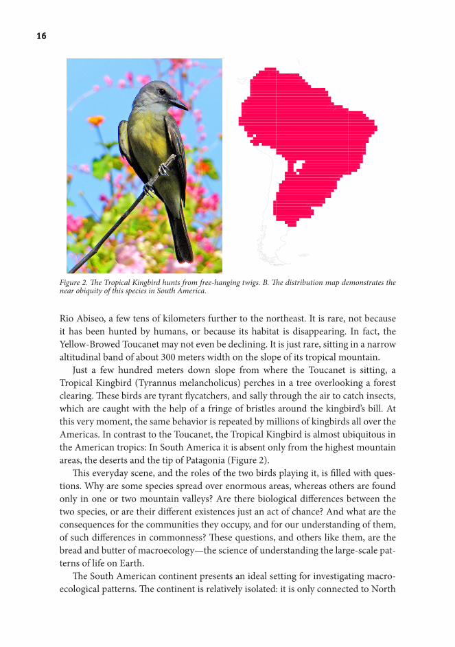
Figure 1. A. A rare picture of the Yellow-browed Toucanet. B. The area of occurrence of the species, in the western part of Peru.
SynopsisMichael K. BorregaardCenter for Macroecology, Evolution and Climate, University of Copenhagen
THE.MACROECOLOGY.OF.SOUTH.AMERICAN.BIRDS
In the small cloud forest site of La Libertad, in North Central Peru on the eastern slope of the Andes, a Yellow-browed Toucanet (Aulacorhynchus huallagae, Figure 1) is preening its feathers. This spectacular bird lives off fruits and small vertebrates that it hunts in the low and moist canopy. As it stops preening, it quietly takes off after a small lizard appearing on a nearby tree.
The Yellow-browed Toucanet is one of the world’s rarest birds. It is known only from two localities worldwide, the extremely remote type locality here in La Libertad (Schulenberg & Parker 1997), and as a small population at the world heritage site of
1616
SouthAmerica_current
1
Figure 2. The Tropical Kingbird hunts from free-hanging twigs. B. The distribution map demonstrates the near obiquity of this species in South America.
Rio Abiseo, a few tens of kilometers further to the northeast. It is rare, not because it has been hunted by humans, or because its habitat is disappearing. In fact, the Yellow-Browed Toucanet may not even be declining. It is just rare, sitting in a narrow altitudinal band of about 300 meters width on the slope of its tropical mountain.
Just a few hundred meters down slope from where the Toucanet is sitting, a Tropical Kingbird (Tyrannus melancholicus) perches in a tree overlooking a forest clearing. These birds are tyrant flycatchers, and sally through the air to catch insects, which are caught with the help of a fringe of bristles around the kingbird’s bill. At this very moment, the same behavior is repeated by millions of kingbirds all over the Americas. In contrast to the Toucanet, the Tropical Kingbird is almost ubiquitous in the American tropics: In South America it is absent only from the highest mountain areas, the deserts and the tip of Patagonia (Figure 2).
This everyday scene, and the roles of the two birds playing it, is filled with ques-tions. Why are some species spread over enormous areas, whereas others are found only in one or two mountain valleys? Are there biological differences between the two species, or are their different existences just an act of chance? And what are the consequences for the communities they occupy, and for our understanding of them, of such differences in commonness? These questions, and others like them, are the bread and butter of macroecology—the science of understanding the large-scale pat-terns of life on Earth.
The South American continent presents an ideal setting for investigating macro-ecological patterns. The continent is relatively isolated: it is only connected to North

17Synopsis 17Synopsis
SouthAmerica_current
275380
106133157186212238265291317344371397423450476503529554582603630657682
709754
793847
SouthAmerica_current
275380
106133157186212238265291317344371397423450476503529554582603630657682
709754
793847
Figure 3: A map of the species rich-ness of birds in South America. The continent is divided into squares of 1x1 degree of latitude and longitude. In each square, the number of spe-cies is counted, and expressed by the color code shown at the left. Red colors indicate a very high number of species, whereas dark blue indi-cates a very low number.
America along a narrow strip of land in the northwest corner, which closed about 3.5 million years ago. This makes it feasible to treat South America as one self-contained unit. It spans from the northern hemisphere tropics down to the temperate regions of the south, encompassing huge areas of both savannah-like lands and rainforest. Two biomes in South America are especially conspicuous and charismatic: the vast rainforest basin of Amazonia, and the Andes mountain range, which spans the entire length of the continent, and reaches almost 7000 meters of altitude. South America also contains a uniquely rich fauna of mammals, of amphibians—and of birds, the group that I focus on within this thesis.
The eastern Andean slope towards the Amazon basin is among the most species rich places on Earth. In a single square, measuring just over 100kms on each side, close to Quito in Ecuador, a sufficiently persistent bird watcher could see more than 800 different species of birds, equivalent to one tenth of all bird species on the planet! If this bird watcher moved into the Amazon itself, the number of species he would see would drop dramatically. Should his travels bring him to the Atacama desert in northwestern Chile, he could see no more than 20 bird species in an area of the same size, most of which he would have already seen before. If we could see species rich-ness directly, as if from a place far over the continent, we would see a pattern of very pronounced variation. This variation can be visualized using color-coded maps such as that in figure 3. The reasons for this geographic variation in species richness have

1818
Figure 4: The elephant and the six blind men.
occupied scientists since the days of von Humboldt, but are still not completely un-derstood.
In current ecology, most explanations for this variation in species richness as-sume that it is controlled by climatic factors such as temperature. Climate analyses, in which the number of species in a sampling square are compared to the amount of incoming solar energy or plant productivity, invariably show very strong correlations (Currie 1991). The many explanations for this correlation range from the idea that higher plant productivity allows more individuals to share an area (Wright 1983), to the recent idea that incoming energy directly affects the speed of individual metabo-lism and hereby the rate of evolution (Allen et al. 2002).
An added complexity, though, is that species distributions and richness patterns have a long history. It is increasingly realized that historical factors, such as conti-nental tectonics and climatic history, should also be taken into account when deal-ing with geographical patterns (Wiens & Donoghue 2004). As an example, in South America, many birds are adapted to specific altitudinal zones in the Andes. During historical ice ages, these zones have moved up and down the mountains, potentially isolating and reconnecting species populations, and thus creating opportunities for allopatric speciation (Fjeldsa 1994). Trying to combine these views, and reach a con-sensus understanding of large-scale species patterns, is the challenge for macroecol-ogy.

19Synopsis
METHODOLOGICAL.FRAMEWORK
The goal of macroecology is not just to explain large-scale ecological patterns. Rather, the goal is to use these patterns to understand how ecological processes, such as e.g. ecological speciation or niche dynamics, shape large-scale species patterns. In classi-cal biology, the silver bullet for uncovering processes is the controlled experiment. A classic example of this is the Park Grass experiment at Rothamstead, where fertiliz-ers of different kinds were added to plots over many decades, while other plots were unfertilized (Brenchley & Warington 1958). Because plots were selected to be similar at the outset, later differences between fertilized and control plots were very strong indicators of the effect of fertilization.
At the scales of macroecology and biogeography, however, experiments are usu-ally not possible—they would be prohibitively expensive, and there would also be serious ethical concerns when changing landscapes at so large scales. This means that we must infer our knowledge about processes from the patterns we can observe in nature.
A traditional Indian story, popularized in English by Sir John Godfrey Saxe, tells of 6 blind men touching an elephant (Figure 4). Each man touches a different part of the elephant: The side, the tusks, the trunk, the knee, the ears and the tail. Having only their sense of touch to go by, each man has a very different impression of what an elephant is like, and they start arguing about who of them has the right ‘elephant-view’. Even if these men were wise enough to realize that they perceive different parts of the elephant and start working together, it would still be a formidable task for them to construct a coherent image of the whole elephant.
In having to use observed patterns to uncover the processes shaping species pat-terns on continents, macroecologists are in the same situation as these blind men. One scientist holds a strong relationship between plant productivity and tempera-ture, whereas another is grasping the observation that most species are adapted to warm climates because of their evolutionary history. Fortunately, scientists work together and we have some idea of how the elephant could look; but the image is far from clear. This situation puts great emphasis on developing conceptually sound analytical methods, and strains our creativity for integrating the knowledge we have in new frameworks.
Null.models
A major challenge for inferring process from patterns is that we do not have controls to show the pattern that appears in the absence of a given process. In some cases this is trivial, but for many questions in macroecology, it is far from obvious. A classic ex-ample is the average number of species per genus, which has been used as a measure of the degree of competition in animal communities (Elton 1946). However, what is the expected species/genus ratio in the absence of competition?

2020
One way of dealing with this issue is to create a reference pattern using a ‘null’ model. A null model is a model that uses randomization procedures to create the pattern that would be expected in the absence of a particular mechanism (Gotelli & Graves 1996). In one of ecology’s earliest null models, Williams (1947) used random draws from a species pool to show that species/genus ratios are expected to vary with species richness, simply for reasons of chance sampling. Revisiting Elton’s (1946) analysis, Williams then refuted his original conclusions about the levels of competi-tion in islands.
The debate did not end there, and the two papers by Elton and Williams sparked considerable controversy, that lasted in the scientific debate for decades (Gotelli & Graves 1996). Such controversy has characterized the use of null models, which has been at the center of several heated debates in the ecological literature (e.g. Connor & Simberloff 1979; Diamond & Gilpin 1982). This is not only because they often lead to interpretations of ecological patterns that diverge from intuition or conventional wis-dom, but also because null models are inherently difficult to design so they only differ from the empirical system with respect to the focal process. In addition, the approach contrasts with traditional statistical methods that emphasize the use of completely non-informative null hypotheses. Nevertheless, null models remain a valuable tool for investigating the ecological relevance of observed patterns.
In macroecology, one of the most widely used null models is probably the ‘spread-ing dye’ model of Jetz and Rahbek (2001; building on an earlier model by Colwell & Hurtt 1994). This model aims to answer the question “what would the pattern of species richness be if species were not affected by local environmental factors”. The null model itself consists of a computer algorithm, which places simulated ranges as cohesive areas on a model version of the study area. It then counts the number of overlapping ranges, to yield null predictions of species richness. This process has been likened to piling pancakes on a large plate and then pushing a measuring stick through the layer at regular intervals, to create a ‘pancake-thickness pattern’ (N. Go-telli, pers comm.).
In the present thesis, I have used null models in several contexts. One example was a study of range size patterns in European flatworms (Appendix I), in which the sampling units were the freshwater biogeographical regions of Europe. These sam-pling units have irregular shapes and sizes, which creates a bias in the geographical pattern of range sizes. To accommodate this problem, I applied a modification of the spreading dye algorithm, by randomly picking contiguous biogeographical regions to generate a reference pattern. Because this pattern was based on the same sampling units as the empirical data, the reference pattern reflected the same bias as the em-pirical pattern, and comparisons between the two should be unbiased.

21Synopsis
Simulations
A different solution to the problem of uncovering processes in non-experimental systems is to create a simulation. A simulation is an artificial system that explicitly models processes of interest in a stochastic environment, and lets the researcher in-vestigate the consequences of different scenarios (Peck 2004; Grimm et al. 2005). Simulations have been performed for decades, by drawing cards or using colored balls; for example, throwing rice grains on a gridded board simulates a Poisson spa-tial process. In addition, mathematical models that incorporate random variables are a type of simulation. However, the rise of computer technology has revolutionized the contribution of simulations to scientific enquiry, also in the field of ecology.
Simulation models can be very simple, like the example using rice grains above. Such simulations are conceptually easy to grasp, and provide strong tools for evaluat-ing the effect of single processes. The flip side is that these simple models lack realism, as natural systems are usually complex (Grimm et al. 2005). At the other end of the continuum, there are simulations so complex that they become systems for sampling and pattern analysis themselves (Peck 2004); the increased realism of such complex models thus comes at a loss of conceptual transparency. For this reason, I have fo-cused on simple simulation models in the present thesis.
DETERMINANTS.OF.GEOGRAPHICAL.RANGE.SIZES
The aim of the present thesis is to investigate the links between geographic ranges and observed patterns in macroecology. The investigation falls naturally into two thematic components: how ecology and evolution determine species’ ranges; and, conversely, how range characteristics shape ecological processes and patterns. In the following, I will go through each of those components and show how they were ad-dressed by the thesis chapters.
In addition to these two components, the conceptual basis for working with spa-tial patterns in ecology is laid out in a book chapter, which has been published as part of Elsevier’s recent Encyclopedia of Ecology (chapter 5). The chapter is written at a level suitable for undergraduate students, and introduces the notion of spatial pat-terning and its consequences for ecology. Following the spatial scale of processes as a framework, the chapter covers the basic theory of spatial ecology, such as aggregation patterns, metapopulation dynamics, predator-prey co-occurrence, flocking behavior and finally large-scale range dynamics.
The first thematic component deals with the ecological and evolutionary determi-nants of species ranges. The basic attribute of species ranges is their size, which can be measured as the extent of the region where the species can be found, or by some measure of the area actually occupied by individuals of the species (Gaston 1991).
2222
Though the determinants of geographical range sizes have been studied for decades (Willis 1926; Brown et al. 1996), they are still the object of vivid debate (Bohning-Gaese et al. 2006). Here, I take first an ecological and then an evolutionary approach to geographic range sizes.
The.distribution-abundance.relationship
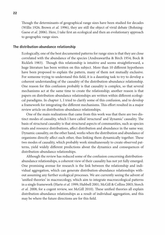
Ecologically, one of the best documented patterns for range sizes is that they are close correlated with the abundance of the species (Andreawartha & Birch 1954; Bock & Ricklefs 1983). Though this relationship is intuitive and seems straightforward, a huge literature has been written on this subject. More than 10 different hypotheses have been proposed to explain the pattern, many of them not mutually exclusive. For someone trying to understand this field, it is a daunting task to try to develop a coherent understanding of the causality of the distribution-abundance relationship. One reason for this confusion probably is that causality is complex, so that several mechanisms act at the same time to create the relationship; another reason is that papers on distribution-abundance relationships are written within different ecologi-cal paradigms. In chapter 1, I tried to clarify some of this confusion, and to develop a framework for integrating the different mechanisms. This effort resulted in a major review article on distribution-abundance relationships.
One of the main realizations that came from this work was that there are two dis-tinct modes of causality, which I have called ‘structural’ and ‘dynamic’ causality. The basis of structural causality is that structural aspects of communities, such as species traits and resource distributions, affect distribution and abundance in the same way. Dynamic causality, on the other hand, works when the distribution and abundance of organisms directly affect each other, thus linking them dynamically together. These two modes of causality, which probably work simultaneously to create observed pat-terns, yield widely different predictions about the dynamics and consequences of distribution-abundance relationships.
Although the review has reduced some of the confusion concerning distribution-abundance relationships, a coherent view of their causality has not yet fully emerged. One promising avenue for research is the link between the relationship and indi-vidual aggregation, which can generate distribution-abundance relationships with-out assuming any further ecological processes. We are currently seeing the advent of ‘unified theories’ in macroecology, which aim to integrate macroecological patterns in a single framework (Harte et al. 1999; Hubbell 2001; McGill & Collins 2003; Storch et al. 2008; for a cogent review, see McGill 2010). These unified theories all explain distribution-abundance relationships as a result of individual aggregation, and this may be where the future directions are for this field.

23Synopsis
Ranges.and.species-level.heritability
It is said that nothing in biology makes sense except in the light of evolution (Do-bzhansky 1964). The species traits that determine range sizes, such as habitat associa-tions and dispersal ability, are exposed to natural selection pressures, and thus under constant evolution. But are ranges themselves affected by selection processes?
The catch here is that range traits, such as range size, are attributes of the whole species. Such emergent traits differ from aggregate traits like body size, which char-acterize individuals: the body size of a species is really a statistical distribution of the sizes of each individual organism. Therefore, emergent traits are not subject to classi-cal natural selection, which operates at the level of individuals. However, it has been argued that emergent traits might be influenced by higher-level selection processes operating at the species level (Jablonski 1987; Diniz-Filho 2004).
Species-level selection is highly controversial, though theoretically feasible. In or-der for a trait to respond to classical Darwinian selection, there must be differential reproduction or survival of individuals with that trait, and the trait must be heritable. Correspondingly, an emergent trait could be subject to species-level selection if it co-varies with speciation or extinction rates, and is inherited from ancestor to de-scendant species (Lewontin 1970). The first criterion is fulfilled, as small geographic range size is associated with elevated extinction rates (McKinney & Lockwood 1999). Thus, the key element for species selection processes to be feasible is whether there is a type of heritability at the species level, transferring traits from ancestor to descen-dant species.
Testing range-size heritability is very difficult, because data are scarce: There is no easy way to estimate the range sizes of ancestral species that are now extinct. In chapter 2, I addressed this difficulty by using simulation. Based on a study of range size heritability by Jablonski (1987), I constructed a simulation model that modeled the evolution of range sizes on phylogenetic trees. I then compared the range size distributions generated at different levels of heritability to the empirical ranges of South American birds. The correspondence to the empirical data was closer when in-corporating relatively high levels of heritability in the models. This result is consistent with the idea of range-size heritability, and indicates a potential role for species-level processes in shaping current range-size distributions.
THE.ROLE.OF.RANGES.IN.GENERATING.MACROECOLOGICAL.PATTERNS
The study of ecological and evolutionary determinants of geographic ranges has a long history (Grinnell 1917; Willis 1926). It has much more recently been recognized that geographic ranges determine patterns in ecology as well (Colwell & Hurtt 1994). Analytically, species-area curves, spatial turnover and the pattern of geographic vari-

2424
ation in species richness are all emergent properties of the spatial location of geo-graphic ranges and the numerical distribution of species’ range sizes.
The species richness value for a site is just a count of the species occurring there. But the species there may be very different: Some sites have species that are localized and only exist in the surrounding area, whereas others have as many species that are all widespread and occur everywhere. Such patterns in species composition, and the level of similarity with nearby regions, are hidden in basic maps of species richness.
One way to visualize these patterns is to generate site ‘dispersion fields’ (Graves & Rahbek 2005). Technically, a dispersion field is created by overlapping the range maps of all species occurring in a site (Figure 5). The resulting richness map has a maximum value at the focal site and then decreases with distance away from this site. Sites with high values have high compositional similarity to the focal cell, and it has been argued that the contours of the plots indicate the geometric shape of species source pools (Graves & Rahbek 2005), a concept which has otherwise been consis-tently difficult to pin down in community ecology. In two chapters of this thesis, I explore the utility of dispersion fields for evaluating the importance of species ranges for ecological patterns.
SouthAmerica_current
5
6789
10
11121314
15
1617192225283031323437416189
103
SouthAmerica_current
5
6789
10
11121314
15
1617192225283031323437416189
103
Figure 5. The dispersion field of the square shown in dark red color, in the highest region of the Andes. The color scale is an equal frequency scale, to illustrate the de-gree of similarity between the composition of the focal square and all other squares in South America. The number next to the color bar indicates the number of species each grid cell shares with the focal cell.It is clear that many of the birds that occur in the focal cell also occurs elsewhere in the Andes, whereas only very few are also found in the Amazon.

25Synopsis
.Asymmetric.dispersion.fields.and.the.signature.of.biomes
One exciting application for dispersion fields is to enhance our understanding of the processes that lead to geographic variation in species richness. Most mechanisms proposed to explain species richness patterns are based on processes that occur in situ at the sample site, such as the influence of water and temperature on primary production (Hawkins et al. 2003). Such site-based approaches have been termed ‘ver-tical’ by Ricklefs (2008), because they ignore that ecological processes occur over the entire extent of species’ ranges, which are ‘horizontal’ in space. Ricklefs (2008) then argues convincingly for an approach to spatial ecology that is based on horizontal patterns.
Dispersion fields are a way to visualize the horizontal structure in continental assemblages. Such structure could be created by the distribution of vegetation types and the spatial configuration of different biomes. If biomes constrain the potential distributions of species, they should leave characteristic signatures on the shape of dispersion fields.
In chapter 4, I demonstrated a clear spatial pattern in the asymmetry of disper-sion fields for South American birds. When excluding the 25% most common species that occur almost everywhere, dispersion fields were oriented towards the center of the biogeographic region of the focal cell. This result indicates that biogeographic boundaries constrain the distributions of species and thus determine the species pool which is available for local assembly processes. Hence, a comprehensive theory of biodiversity must combine both horizontal and vertical approaches.
Dispersion.fields.and.range.covariance
Another use of dispersion fields is to use them for visualizing covariance in spe-cies distributions, using specialized range-diversity plots (Arita et al. 2008). Range-diversity plots have the species richness of sites on the y axis, and the mean range of all species occurring at the site on the x axis – a simplified dispersion field. A com-plementary type of range-diversity plots has the range sizes of species on the y axis, and the mean richness of all sites occupied by the species on the x axis (which Arita et al. named the ‘diversity field’). Arita et al. (2008) embellished these plots with iso-covariance lines, that connect points with the same degree of covariance.
The main difficulty with range-diversity plots is that they are not easy to inter-pret. The points create characteristic shapes, and seem to some degree to follow the iso-covariance lines. However, it is not clear which patterns are expected from defi-nite scenarios, and there is no null expectation for point dispersion. In a technical commentary, I addressed this issue by applying a set of null models, making explicit the expectations for range-diversity plots within defined circumstances (chapter 3). With these null models, I demonstrated that several patterns, which had been taken by Arita et al. as indicative of ecological processes, were expected merely as a con-sequence of the numerical distributions of the data. The analysis also highlighted
2626
patterns which were clearly different from the null expectation, and which would be fruitful to analyze further.
The very different chapters of this thesis thus weave several aspects of geographic ranges, and their link to biodiversity, into a motif with many details. Combining di-verse conceptual and analytical approaches, a common thread through the chapters is a conviction that geographical ranges are an essential part of any coherent theory of large-scale ecology and biogeography. Enjoy the reading!
REFERENCES
Allen A.P., Brown J.H. & Gillooly J.F. (2002). Global Biodiversity, Biochemical Kinetics, and the Energetic-Equivalence Rule. Science, 297, 1545-1548.
Andreawartha H.G. & Birch L.C. (1954). The distribution and abundance of animals. University of Chicago Press Chicago.
Arita Héctor T., Christen J.A., Rodríguez P. & Soberón J. (2008). Species diversity and distribu-tion in presence-absence matrices: Mathematical relationships and biological implications. The American Naturalist, 172, 519-532.
Bock C.E. & Ricklefs R.E. (1983). Range size and local abundance of some North American songbirds: A positive correlation. American Naturalist, 122 295-299.
Bohning-Gaese K., Caprano T., van Ewijk K. & Veith M. (2006). Range size: Disentangling cur-rent traits and phylogenetic and biogeographic factors. American Naturalist, 167, 555-567.
Brenchley W.E. & Warington K. (1958). The Park Grass plots at Rothamsted 1856–1949. Ro-thamsted Experimental Station, Harpenden.
Brown J.H., Stevens G.C. & Kaufman D.M. (1996). The geographic range: Size, shape, boundar-ies, and internal structure. Annual Review of Ecology and Systematics, 27, 597-623.
Colwell R.K. & Hurtt G.C. (1994). Nonbiological Gradients in Species Richness and A Spurious Rapoport Effect. American Naturalist, 144, 570-595.
Connor E.F. & Simberloff D. (1979). The assembly of species communities: chance or competi-tion? Ecology, 60, 1132-1140.
Currie D.J. (1991). Energy and large-scale patterns of animal-species and plant-species richness. American Naturalist, 137, 27-49.
Diamond J.M. & Gilpin M.E. (1982). Examination of the null model of connor and simberloff for species co-occurrences on islands. Oecologia, 52, 64-74.
Diniz-Filho J.A.F. (2004). Macroecology and the hierarchical expansion of evolutionary theory. Global Ecology and Biogeography, 13, 1-5.
Dobzhansky T. (1964). Biology, molecular and organismic. Am. Zool., 4, 443-452.
Elton C. (1946). Competition and the structure of ecological communities. Journal of Animal Ecology, 15, 54-68.

27Synopsis
Fjeldsa J. (1994). Geographical patterns for relict and young species of birds in africa and south-america and implications for conservation priorities. Biodiversity and Conservation, 3, 207-226.
Gaston K.J. (1991). How large is a species geographic range. Oikos, 61, 434-438.
Gotelli N.J. & Graves G.R. (1996). Null models in ecology. Smithsonian Institution Press, Wash-ington D.C., USA.
Graves G.R. & Rahbek C. (2005). Source pool geometry and the assembly of continental avifau-nas. Proceedings of the National Academy of Sciences, 102, 7871-7876.
Grimm V., Revilla E., Berger U., Jeltsch F., Mooij W.M., Railsback S.F., Thulke H.H., Weiner J., Wiegand T. & DeAngelis D.L. (2005). Pattern-Oriented Modeling of Agent-Based Complex Systems: Lessons from Ecology. Science, 310, 987-991.
Grinnell J. (1917). Field tests of theories concerning distributional control. American Naturalist, 51, 115-128.
Harte J., Kinzig A. & Green J.L. (1999). Self-similarity in the distribution and abundance of spe-cies. Science, 284 334-336.
Hawkins B.A., Field R., Cornell H.V., Currie D.J., Guegan J.F., Kaufman D.M., Kerr J.T., Mit-telbach G.G., Oberdorff T., O’Brien E.M., Porter E.E. & Turner J.R.G. (2003). Energy, water, and broad-scale geographic patterns of species richness. Ecology, 84, 3105-3117.
Hubbell S.P. (2001). The Unified Neutral Theory of Biodiversity and Biogeography. Princeton Uni-versity Press, Princeton, NJ.
Jablonski D.A.V.I. (1987). Heritability at the Species Level: Analysis of Geographic Ranges of Cretaceous Mollusks. Science, 238, 360-363.
Jetz W. & Rahbek C. (2001). Geometric constraints explain much of the species richness pat-tern in African birds. Proceedings of the National Academy of Sciences of the United States of America, 98, 5661-5666.
Lewontin R.C. (1970). The Units of Selection. Annual Review of Ecology and Systematics, 1, 1-18.
McGill B. & Collins C. (2003). A unified theory for macroecology based on spatial patterns of abundance. Evolutionary Ecology Research, 5, 469-492.
McGill B.J. (2010). Towards a unification of unified theories of biodiversity. Ecology Letters, 13, 627-642.
McKinney M.L. & Lockwood J.L. (1999). Biotic homogenization: a few winners replacing many losers in the next mass extinction. Trends in Ecology & Evolution, 14, 450-453.
Peck S.L. (2004). Simulation as experiment: a philosophical reassessment for biological model-ing. Trends in Ecology & Evolution, 19, 530-534.
Ricklefs Robert E. (2008). Disintegration of the Ecological Community. The American Natural-ist, 172, 741-750.
Schulenberg T.S. & Parker T.A. (1997). Notes on the Yellow-Browed Toucanet Aulacorhynchus huallagae. Ornithological Monographs, 717-720.
Stevens G.C. (1989). The Latitudinal Gradient in Geographical Range - How So Many Species

28
Coexist in the Tropics. American Naturalist, 133, 240-256.
Storch D., Sizling A.L., Reif J., Polechova J., Sizlingova E. & Gaston K.J. (2008). The quest for a null model for macroecological patterns: geometry of species distributions at multiple spa-tial scales. Ecology Letters, 11, 771-784.
Wiens J.J. & Donoghue M.J. (2004). Historical biogeography, ecology and species richness. Trends in Ecology & Evolution, 19, 639-644.
Williams C.B. (1947). The generic relations of species in small ecological communities. Journal of Animal Ecology, 16, 11-18.
Willis J.C. (1926). Age and Area. Q. Rev. Biol., 1, 553-571.
Wright D.H. (1983). Species-energy theory - an extension of species-area theory. Oikos, 41, 496-506.

Chapter 1:Causality of the relationship between
geographic distribution and species abundance
Published as:Borregaard, M. K. and Rahbek, C. 2010. Causality of the
relationship between geographic distribution and species abundance. The Quarterly Review of Biology 85(1): 3-25

31
THE QUARTERLY REVIEW
of Biology
CAUSALITY OF THE RELATIONSHIP BETWEEN GEOGRAPHICDISTRIBUTION AND SPECIES ABUNDANCE
Michael Krabbe BorregaardCenter for Macroecology, Evolution and Climate, Department of Biology, University of Copenhagen,
2100 Copenhagen Ø, Denmark
e-mail: [email protected]
Carsten RahbekCenter for Macroecology, Evolution and Climate, Department of Biology, University of Copenhagen,
2100 Copenhagen Ø, Denmark
e-mail: [email protected]
keywordsdistribution-abundance relationships, range-abundance, occupancy-abundance,
distribution-density, macroecology, spatial scale
abstractThe positive relationship between a species’ geographic distribution and its abundance is one of ecology’s
most well-documented patterns, yet the causes behind this relationship remain unclear. Although manyhypotheses have been proposed to account for distribution-abundance relationships, none have attainedunequivocal support. Accordingly, the positive association in distribution-abundance relationships isgenerally considered to be due to a combination of these proposed mechanisms acting in concert. In thisreview, we suggest that much of the disparity between these hypotheses stems from differences in terminologyand ecological point of view. Realizing and accounting for these differences facilitates integration, so thatthe relative contributions of each mechanism may be evaluated. Here, we review all the mechanisms thathave been proposed to account for distribution-abundance relationships, in a framework that facilitates acomparison between them. We identify and discuss the central factors governing the individual mecha-nisms, and elucidate their effect on empirical patterns.
The Quarterly Review of Biology, March 2010, Vol. 85, No. 1
Copyright © 2010 by The University of Chicago Press. All rights reserved.
0033-5770/2010/8501-0001$15.00
Volume 85, No. 1 March 2010
3

32
Introduction
THE POSITIVE RELATIONSHIP be-tween the geographic distribution and
abundance of organisms is a recurrent pat-tern in ecology (Figure 1 and 2) (Andreawar-tha and Birch 1954; Bock and Ricklefs 1983;Brown and Maurer 1989). Published associ-ations between the two variables are dispar-ate, in part reflecting the diversity of meth-ods used to measure distribution orabundance (Wilson 2008). Likewise, manydifferent mechanisms for governing the un-derlying relationship have been proposed.Here, we group these associations under theoverall term distribution–abundance relation-ships, and argue that, although they may have“multiple forms” (Gaston 1996; Blackburn etal. 2006), these associations constitute a sin-
gle overall phenomenon. In this unifyingcontext, we emphasize the impact of anygiven study’s ecological viewpoint on the per-ception of underlying mechanisms. Themechanisms governing the distribution-abundance relationship act at different spatialscales and on different aspects of distribu-tion and abundance, and a considerationof the differential impact of each individ-ual mechanism is necessary for a coherentunderstanding of the mechanistic basis ofthese relationships.
The empirical evidence for a positive asso-ciation between measures of the distributionand abundance of organisms is strong. Posi-tive correlations have been demonstrated fora host of taxa, including birds (e.g., Lacy andBock 1986), butterflies (e.g., Pollard et al.
Figure 1. Intraspecific Distribution-Abundance RelationshipsA) Shows the spatial location of individuals of a species. For clarity, we demonstrate sampling with uniform
grid cells; alternatives include distributed sampling quadrates, or sites defined by habitat characteristics.B) Distribution and abundance are measured, as the presence/absence and population number in each gridcell. On a larger grid (overlaid), the central areas have larger grid cell occupancy. C) The spatial intraspecificrelationship: There is a positive correlation between the cell occupancy and mean local abundance across areasfrom different parts of the range. D) Depicts the same species sampled at a later point in time where thepopulation size has decreased. E) Repeating the sampling process gives a measure of distribution andabundance at this time. F) The temporal intraspecific relationship: integrating the data from (B) and (E)reveals a positive correlation between the distribution and abundance across time.
4 Volume 85THE QUARTERLY REVIEW OF BIOLOGY
NB
: Thi
s figu
re h
as b
een
mod
ified
, by
repl
acin
g th
e bl
ack/
whi
te p
rinte
d fig
ure
with
the
colo
r ver
sion
pub
lishe
d as
supp
lem
enta
ry m
ater
ial.
Intra-speci�c spatial
centre square
edge squares
Number of occupied cells
Mea
n ab
unda
nce
per c
ell
time 2
time 1
Number of occupied cells
Mea
n ab
unda
nce
per c
ell
Intra-speci�c temporal
F
CBA
ED
Time
33
1995; Conrad et al. 2001), mammals (e.g.,Blackburn et al. 1997), and protists (e.g.,Holt et al. 2002b); a few studies have alsobeen published on plants (e.g., Thompsonet al. 1998; Guo et al. 2000). Although moststudies have focused on the terrestrialbiome, relationships between distributionand abundance have also been reported inboth marine (Foggo et al. 2003) and lim-netic (Tales et al. 2004; Heino 2005) biomes,and they have been documented in areasacross the planet (although with an overrep-resentation of northern temperate regions;for a meta-analysis, see Blackburn et al.2006). Distribution–abundance relation-ships have been identified over a large rangeof spatial scales, from micro-invertebrates inmoss fragments on rocks (Gonzalez et al.1998) to birds from the entire North Amer-ican continent (Brown and Maurer 1987).Indeed, although exceptions do occur (e.g.,Johnson 1998; Paivinen et al. 2005; Reif et al.2006; Symonds and Johnson 2006), distribu-tion-abundance relationships are so generalthat they have been proposed as a candidatefor an empirical ecological “rule” (Gastonand Blackburn 2003).
Several hypotheses have been proposed to
explain the processes linking distributionand abundance (Table 1). However, diver-sity in terminology and ecological viewpointhas made a straightforward evaluation ofthese hypotheses difficult, and little consen-sus currently exists regarding the mechanis-tic basis of observed distribution–abundancepatterns (Gaston et al. 2000).
Up until the beginning of the 1990s, thecentral tenet was that some species had evo-lutionary adaptations that made them moresuccessful than others, enabling them toboth establish a wide range and a large pop-ulation size (McNaughton and Wolf 1970;Bock 1987). One of the most influentialhypotheses to explain this superiority wasoriginally put forward by Brown (1984) (seeTable 1, “resource use”), who related distri-bution and abundance to the size of the eco-logical niche of species. Analytical studiesfrom this period generally addressed the ef-fects of the distribution of resources and hab-itat on the distribution and abundance ofspecies (e.g., O’Connor 1987; Gaston andLawton 1990; Novotny 1991).
A different perspective, founded in popu-lation ecology, was introduced when Hanskiand colleagues (1991a; Hanski et al. 1993)
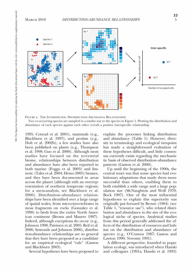
Figure 2. The Interspecific Distribution-Abundance RelationshipTwo co-occurring species are sampled in a similar way to the species in Figure 1. Plotting the distribution and
abundance of each species against each other reveals a positive interspecific relationship.
March 2010 5DISTRIBUTION-ABUNDANCE RELATIONSHIPS
Species 1
Species 2
sp 2
sp 1
Number of occupied cells
Mea
n ab
unda
nce
per c
ell
Inter-speci�c
Sp 2
Sp 1Sp 1
NB
: Thi
s figu
re h
as b
een
mod
ified
, by
repl
acin
g th
e bl
ack/
whi
te p
rinte
d fig
ure
with
the
colo
r ver
sion
pub
lishe
d as
supp
lem
enta
ry m
ater
ial.

34
TABLE 1Proposed hypotheses
Mechanisms/Effects Original explanationDistribution
measure Causality Reference Comment
Measurement effectsSampling bias Species with low abundances are
more likely to be missed bycensuses, thus theirdistributions areunderestimated.
Occupied sites A Bock andRickleffs (1983)
Not a mechanism
Phylogeny Species traits, such asdistribution and abundance,are not independent, andmay reflect phylogeny ratherthan ecology.
N/A N/A Gaston andLawton (1997)
Only interspecificrelationships;not supported
Range position If the study area overlapsdifferent parts of speciesranges, intraspecific spatialrelationships will lead tointerspecific relationships.
Range density N/A Brown (1984) Not a biologicalmechanism
Structural mechanismsResource use Species that are able to exploit a
broader range of resourcesmay acquire larger rangesand also be more locallyabundant, as they will havemore resources available tothem where they occur.
Potential habitat B Brown (1984) Ambiguousempiricalsupport
Resource availability Species that utilize abundantand widespread resourcesmay themselves becomeabundant and widespread.
Potential habitat B Hanski et al.(1993)
See text
Vital rates The local abundance and thenumber of occupied sites ofspecies are both determinedby rates of births and deathsamong populations: Highpopulation growth rate leadsto high abundance, as well asto more sites with a positiveabsolute growth.
Occupied sites B Holt et al.(1997)
See text
Unified theory If the spatial structure ofabundance follows amonotonically decreasingrelationship from the centerof a species’ distribution, theextent of the range (i.e., thearea where abundance � 0)is larger for more abundantspecies.
Extent B McGill andCollins (2003)
Distributionmeasure notempiricallysupported
continued
6 Volume 85THE QUARTERLY REVIEW OF BIOLOGY

35
TABLE 1(continued)
Mechanisms/Effects Original explanationDistribution
measure Causality Reference Comment
Dynamic mechanismsMetapopulation
dynamicsThe number of occupied patches
and local abundance bothinfluence the number ofdispersers, which againinfluences both occupancy andabundance.
Occupied sites C Hanski (1991)
Density-dependenthabitat selection
Individuals in populations withhigh densities might be drivenby intraspecific competition toexploit less suitable habitats,thus increasing the occupancyof the population.
Occupied/potentialhabitat
A O’Connor (1987) See text
Habitat dispersal Populations with much availablehabitat may produce sufficientnumbers of successfuldispersers to inflate localabundances.
Occupied sites C Venier andFahrig (1996)
Spatial aggregation/nonindependence
Individualaggregation
A random spatial dispersion ofindividuals leads to acorrelation between localabundance and site occupancy.This relationship isstrengthened when individualsare spatially aggregated.
Range density B/D Wright (1991),Hartley (1998)
Self-similarity The distribution of species is self-similar across a range of scales.Since the density of a speciesequals the range density at thescale where the average numberof individuals per cell equals 1,density and range density will becorrelated across scales.
Range density B/D Harte et al.(1999)
Neutral models Range-abundance relationships areobserved in neutral communitysimulations, but no explicitmechanism has been stated. Thecausal pathway is through spatialaggregation generated bydispersal limitation.
Range density B Bell (2000)
A: One variable causes the other.B: Both variables are controlled by another (unmeasured) variable.C: Both variables affect each other (the effect takes place in the future, since causality can never be simultaneously mutual).D: There is no causality between the variables.
This table lists all of the hypotheses proposed to explain distribution-abundance relationships. Hypotheses publishedbefore 1997 essentially follow Gaston and Lawton (1997).
March 2010 7DISTRIBUTION-ABUNDANCE RELATIONSHIPS

36
argued that the geographic distribution andabundance of a species need not be indepen-dent measures of its ecological success, butinstead could be directly linked to eachother through the action of metapopulationdynamics. At the same time, a statistical per-spective was added to the discussion of dis-tribution–abundance relationships byWright (1991), who pointed out that a ran-dom spatial distribution pattern of individu-als could in itself be predicted to result in acorrelation between the two variables.
These different frameworks were not easyto integrate, and analytical studies formu-lated within one of these hypotheses havetended to ignore the others (e.g,. Nee et al.1991; Venier and Fahrig 1996; Collins andGlenn 1997; Newton 1997; Hartley 1998;Gregory 1998; Gaston et al. 1998b), with thenotable exception concerning a large studyof British birds that attempted to test all ofthe proposed hypotheses (reviewed in Gas-ton et al. 2000). Recently, a number of com-prehensive macroecological theories aimedat explaining the multiplicity of observeddiversity patterns in a single theoreticalframework have also sought to account fordistribution–abundance relationships, nota-bly those of community self-similarity (Harteand Ostling 2001) and neutral theory (Bell2001; Hubbell 2001).
In all, at least thirteen different hypotheseshave been proposed to explain relationshipsbetween distribution and abundance (Table1). The tendency for explanations of generalempirical patterns to accumulate mechanistichypotheses is common in (macro)ecology, andcan probably be attributed to difficulties withapplying strong inference to ecological theo-ries (McGill et al. 2007). The complementarityand overlap between hypotheses of distribu-tion-abundance relationships mean that astrict Popperian approach of generating spe-cific and identifiable predictions from eachhypothesis is not likely to lead to clear-cutempirical tests. In addition, it is very unlikelythat any one of these hypotheses will befound to be correct to the exclusion of theothers (Gaston and Lawton 1997). Themechanisms are not mutually exclusive, andmay often act in concert to give rise to distri-bution-abundance relationships (Cowley et
al. 2001; Holt and Gaston 2003). The con-cept that several mechanisms may be respon-sible for creating general ecological patterns(see Chamberlain 1890) is well-established inthe study of large-scale species richness gra-dients (e.g., Rahbek and Graves 2001; Williget al. 2003; Colwell et al. 2004; Currie et al.2004) as well as species-area curves (Rosenz-weig 1995), as is the observation that therelative importance of factors and their in-teraction may change with spatial scale (e.g.,Rahbek and Graves 2001; Lyons and Willig2002; see Rahbek 2005 for a review).
The central claim of this review is that thedifferent mechanisms underlying distribu-tion-abundance relationships do not consti-tute competing hypotheses to be supportedor refuted; rather, they are descriptions ofprocesses working at different scales and indifferent manners to create and modifythese relationships. The key to moving froma list of potential hypotheses to a coherentview of the causation of distribution-abundance relationships is to consider thefactors that order and differentiate the hy-potheses, in order to develop a frameworkthat allows comparisons to be made (Leiboldet al. 2004). The factors identified in thispaper include spatial scale, type and direc-tion of causality, temporal dynamics, and themeasure of distribution and abundance thatare implicit in each hypothesis. This allianceof factors also serves to differentiate many ofthe primary ecological frameworks andworldviews that constitute contemporaryecological thought.
A Framework forDistribution-Abundance
RelationshipsDistribution-abundance relationships are
studied under a plethora of names: distribu-tion-abundance relationships (Bock 1987;Blanchard et al. 2005), density-distributionrelationships (Cowley et al. 2001; Paivinen etal. 2005), abundance-occupancy (or occu-pancy-abundance) relationships (Gaston etal. 1998b; Freckleton et al. 2006), densityrange-size relationships (Tales et al. 2004),and range size-abundance relationships (Sy-monds and Johnson 2006), just to name afew. While this variety in nomenclature re-
8 Volume 85THE QUARTERLY REVIEW OF BIOLOGY

37
flects the important efforts made to distin-guish precisely among different measuringtechniques, it has also fragmented the liter-ature, and may have prevented importantfindings and theoretical developments fromcoming to the attention of researchers. Ac-cordingly, although accurate nomenclatureis important, different names should only beupheld if they describe clearly separate phe-nomena. Unfortunately, until now it appearsthat the exact choice of wording tends to re-flect each researcher’s individual preference,rather than following an exact nomenclatureaimed at clarifying the measures in use.
Therefore, we propose reverting to the de-liberately general term “distribution-abundance relationships” to indicate anykind of correlation of a measure of rangeand a measure of abundance; more specificterms that do not contribute to the theoret-ical understanding of the pattern should beabandoned. This is the term used when thepattern was originally described (Andreawar-tha and Birch 1954; Brown 1984; Bock1987), and thus provides consistency withthe original literature. This term also allowsfor studies using nontraditional measures ofdistribution and abundance—for instance,the specificity and incidence of parasites onbirds (Poulin 1999)—to be understood inlight of distribution-abundance mechanisms.
Although we propose a general term toencompass all studies relating distributionand abundance, a first priority at the presentstage is to establish a clear consensus on ex-act empirical patterns (Wilson 2008). To thisend, a stringent terminology of distribution-abundance relationships is needed, and thisrequirement should be kept in mind whendefining mechanistic hypotheses.
Measures of AbundancePublished studies of distribution-abundance
relationships have correlated distribution witheither the total population size of the species(e.g., Blackburn et al. 1997; Webb et al. 2007)or the local abundance (i.e., the averageabundance at occupied sites; e.g., Hanski andGyllenberg 1997). The most interesting distri-bution-abundance relationship ecologically isthe relationship between local abundance anddistribution (Figure 3). Because population
size is the product of occupied area and localabundance, a positive correlation betweentotal population size and distribution inevi-tably follows; for distribution and populationsize to be unrelated would require a negativerelationship between distributional size andlocal abundance. Correlations between pop-ulation size and distribution, therefore, donot require any biological explanation.Although some of the hypothesized mecha-nisms of distribution-abundance relation-ships are phrased in terms of population size(e.g., neutral models [Bell 2001] and self-similarity [Harte and Ostling 2001]), thesemechanisms are also expected to lead to cor-relations between local abundance and dis-tribution.
In local scale analyses, abundance can bemeasured directly using site populationcounts (e.g., Bibby et al. 1992). This is thepreferred method of measurement whendata of sufficient quality are available(Blackburn et al. 1997), which may be thecase for certain organisms—typically verte-brates and plants—or where the extent ofthe study area is relatively limited. How-ever, the size of the data set often makes a
Figure 3. The Relationship between LocalAbundance and ProportionalOccupany among Danish Birds
Data taken from the Danish breeding bird Atlas(Grell 1998; for a description of data selection, seeBorregaard and Rahbek 2006) at the 5x5 km scale(black dots), and subsequently resampled by lumpinggrid cells to 25x25 km cells (white dots). The slopesare significantly different (t � 7.14, p � 0.001).
March 2010 9DISTRIBUTION-ABUNDANCE RELATIONSHIPS
38
direct estimation of local abundance im-practical, and, in these cases, local abun-dance is estimated by dividing the totalpopulation size of the given domain by thenumber of occupied sites within that do-main (Gaston and Lawton 1990). Althoughsome studies have estimated local abun-dance by averaging population size overthe entire study area (including unoccu-pied sites—termed the “true mean abun-dance” by Wilson [2008]), this division by aconstant is merely a different scale repre-sentation of total population size; there-fore, the division of population size by thenumber of occupied sites is to be preferred(Gaston and Lawton 1990).
It is important to note that the use of aver-aged local abundances may give rise to a num-ber of issues. Since local abundances aregenerally not normally distributed (McGill etal. 2007), the average value may not accuratelydescribe species abundance at any specificpoint on the landscape and should, thus, beinterpreted with caution. Furthermore, this ap-proach may lead to spurious inference of dis-tribution-abundance relationships. At largegrain sizes, a species usually occupies only aportion of each grid cell. When averagingoccurrences over grid cells, one implicitly as-sumes that the distribution of individuals is uni-form—or at least comparable among differentspecies—within each grid cell. If there are dif-ferences among species distributions withingrid cells (this in itself is a prediction of severalof the proposed hypotheses for distribution-abundance relationships), then studies usingaveraged abundances may in fact be compar-ing the range density at different scales (i.e.,comparing the within-cell occupancy with theacross-cells occupancy; see the discussion ofself-similarity theory below).
Measures of DistributionMeasures of distribution are fundamen-
tally different from measures of abundancein that distributions are spatial patterns;therefore, comparisons between the two vari-ables are not straightforward. Abundancesare counts of individuals within a predefinedarea, whereas the distribution of a species isessentially a representation of the complexspatial distribution of individuals (see Figure
1) (Brown et al. 1996). This is usually mea-sured as the sum of occupied areas and, assuch, is always a function of how areas aredefined and delimited. Much of the confu-sion regarding distribution-abundance rela-tionships comes from the inherent difficultyin relating absolute counts to measurement-dependent distributions.
Importantly, the measurement of species’distributions is strongly dependent upon thescale of extent and the grain size at whichthey are perceived (Hartley and Kunin 2003;Rahbek 2005). Accordingly, the variety ofdistribution definitions used in studies of dis-tribution-abundance relationships is evengreater than those used for abundance (seeGaston 1996; Blackburn et al. 2006; Wilson2008). The empirically supported relation-ship is a correlation of abundance with den-sity of occupied sites or grid cells on arange—a measure termed “range density” byHurlbert and White (2005). The extent ofthe distribution is not very well-correlatedwith local abundance (e.g., Harcourt et al.2005); a recent meta-analysis showed thatstudies using extent as the distribution mea-sure generally report no correlation withabundance (Blackburn et al. 2006). Thiscarries the implication that mechanisms pro-posed to lead only to extent-abundancecorrelations, such as the unified theory ofmacroecology (McGill and Collins 2003), arenot able to account for observed distribu-tion-abundance relationships.
A consequence of the spatial nature ofdistribution measures is that abundance anddistribution are not expected to scale in thesame way. Accordingly, the exact slope ofdistribution-abundance relationships is scale-specific, and can only be compared betweencommunities censused at the same grain size(He and Gaston 2000b) (see Figure 2). Thisis further complicated by the fact that theperception of scale varies between organisms(Wiens 1989; Chust et al. 2003; Rahbek2005). In any one assemblage, the samegrain size is likely to be perceived differentlyby an eagle and a sparrow, for instance(Wiens 1989).
Not all the proposed hypotheses are appli-cable at all scales. Although the exact scale israrely explicitly defined in mechanistic hy-
10 Volume 85THE QUARTERLY REVIEW OF BIOLOGY

39
potheses (Collins and Glenn 1997), many ofthe mechanisms are based on assumptionsthat are characteristic of biological processesoperating at a specific spatial scale of resolu-tion (see Figure 4). Scale issues are of greatimportance. Analyzing a specific mechanistichypothesis that is operational within a givenrange of spatial scales, but using data ob-tained outside of this range to do so, canseriously confound conclusions. For in-stance, applying the hypothesis of density-dependent habitat selection (O’Connor1989) to relationships between the distribu-tion and abundance measured at the spatialresolution of 100x100 km grid cells is clearlyflawed. Individuals dispersing as a result ofdensity dependence are likely to disperseinto lower quality habitat patches that areinterspersed with optimal habitat withinthe landscape matrix, and these individu-als are not likely to affect the distributionof the organism at a larger grain size. Aconverse example would be interpretingdistribution and abundance of butterfliesin a set of closely connected forest patchesby employing the “vital rates” model (Holt
et al. 1997). This model is only applicableat larger scales, where sites may be spacedsufficiently far apart such that dispersal be-tween them can be neglected. Anotherequally important aspect of spatial depen-dency is that some mechanisms, ratherthan acting as competing explanations, de-scribe processes working at different scales.For instance, Brown’s (1984) resource usehypothesis acts at a large landscape scale andaffects the distribution of potential habitatrather than the distribution of individuals,whereas metapopulation dynamics (Hanski,1981) determine the individual occupan-cies in a network of closely connectedpatches and, hence, act at an organismicscale nested within that of the resource usehypothesis (Storch et al. 2008). Regardlessof these scale associations, positive distri-bution-abundance relationships exist overa wide range of scales and display a certaindegree of scale invariance: organisms com-mon and widespread at one scale are gen-erally equally so at any other (e.g., Bock1987).
Another consequence of the spatial na-ture of ranges is that distribution measuresare proportion data (i.e., the proportion ofthe study area that is occupied). Because of
Figure 5. The Effect of Grain Size onMeasured Relationships
Log/log plots of occupancy on total population sizeoften exhibit saturation at large grid cell sizes. Data as inFigure 3. A positive relationship between local abun-dance and distribution is predicted to yield linear slopesof �1 in this type of plot (Blackburn et al. 1997).
Figure 4. Scale Dependency of the ProposedMechanistic Hypotheses
Several of the hypotheses assume biological pro-cesses that are characteristic of a certain spatial scale.For example, meta-population dynamics depend ondispersal between habitat patches and cannot explainpatterns at larger scales, whereas the unified theoryconcerns distributional extent and is only applicableat the largest scales. Individual aggregation modelsindividuals (dotted line) and is traditionally associ-ated with local scales, although this is not a strictassumption of aggregation theory.
March 2010 11DISTRIBUTION-ABUNDANCE RELATIONSHIPS

40
this, the linear trend of log-log plots of dis-tribution on population size often shows aflattening at high population sizes, wheredistribution cannot increase further (Greg-ory 1995; Gaston et al. 1998c; Webb et al.2007). This behavior is caused by the grainsize or focus of the study rather than by theextent (sensu Scheiner et al. 2000); as grainsize decreases, the flattened area moves pro-gressively higher, and the effect almost dis-appears at the smallest grain size (Figure 5).The claim that this flattening is “a real phe-nomenon” (Webb et al. 2007) seems to beinaccurate, as it is actually a measurementeffect of grain size. Smaller variation of mea-sured distributions among abundant speciesis a product of poor resolution in this part ofthe plot. A more appropriate approach is tonormalize the distribution values using logit(logit(p):�log(p/(1�p)) transformation(Hanski and Gyllenberg 1997; Williamsonand Gaston 1999), which generally leads tostronger distribution-abundance relation-ships (Blackburn et al. 2006) and removesthe above effect (Figure 3).
Sampling BiasSpurious relationships between measured
distribution and abundance may be createdby sampling bias. If species with low densitiesare more likely to elude detection at siteswhere they are actually present, they will beregistered at fewer sites than more numer-ous species, and a spurious relationship be-tween distribution and local abundance willresult (Bock and Ricklefs 1983; Brown 1984).This organism-specific sampling effect hasbeen demonstrated in empirical studies(e.g., Selmi and Boulinier 2004) and will al-ways contribute to distribution-abundanceanalyses, especially when sampling intensityis low or is carried out at small spatial scales.However, the generality of distribution-abundance relationships cannot be ascribedonly to the effect of sampling bias; positiverelationships are also found in studies wherethe species inventory in each site is almostcomplete (e.g., Figure 3).
Gaston and Lawton (1997) also sug-gested that distribution-abundance rela-tionships among related species may bebiased by phylogeny, as a result of the phy-
logenetic nonindependence of ecologicaltraits (Harvey and Pagel 1991). However,this postulate has received no empiricalsupport (see Paivinen et al. 2005), andthere is no a priori reason to assume thatphylogeny itself should lead to the infer-ence of spurious distribution–abundancerelationships.
Direction of CausalityCorrelation between two variables indi-
cates the existence of an unresolved causalrelationship (Shipley 2004). This correlationmay indicate that one of the variables causesthe other, that both cause the other overtime, that both are caused by some externallatent (unmeasured) factor, or that the twovariables are merely measures of the sameentity (see Figure 6).
Studies of distribution-abundance pat-terns have plotted both distribution andabundance on the x axis. The low consis-tency with regard to plotting this relation-ship probably reflects a generally assumedconsensus that causality between the twovariables is likely to be bidirectional (e.g.,Bock 1987; Gregory 1998). However, there isno clear empirical evidence supporting this as-
Figure 6. Possible Causal Pathways forDistribution-AbundanceRelationships
A correlation between two variables may indicate A)that one variable causes the other; B) that both arecontrolled by another (unmeasured) variable; C) thatboth variables affect each other (i.e., as causality cannotbe completely mutual, they can only affect each other ata future time [Shipley 2004]); and D) that there is nocausality as such between the variables, as they are justdifferent manifestations of an underlying entity.
12 Volume 85THE QUARTERLY REVIEW OF BIOLOGY

41
sumption, and the mechanistic hypotheses arebased on different assumptions of the causalpattern underlying the distribution-abundancecorrelation (as shown in Table 1).
Clarifying the causal direction of dis-tribution-abundance relationships has im-portant implications within the context ofconservation biology. Arguably, the mostserious threat against the world’s plants andanimal species is habitat destruction (Balmfordand Bond 2005; Jetz et al. 2007). If there is astrong effect of distribution on the abundancethat a species can attain within the distribu-tional range, species experiencing habitat de-struction or range retraction as a result of cli-matic change may actually face a “doublejeopardy” from the combined effects of smalldistribution and low population numbers(Gaston 1998; Johnson 1998). Similarly, spe-cies whose population numbers are dwin-dling as a consequence of human harvest-ing may experience double jeopardy if theinfluence of local abundance on distribu-tion causes the ranges of these species tocollapse (Gaston 1999).
Types of Distribution-AbundanceRelationships
There are at least three types of relation-ships between distribution and abundance(Figure 1): interspecific, intraspecific tempo-ral, and intraspecific spatial relationships. In-terspecific relationships, which are the mostempirically well-supported, refer to a positivecorrelation in a plot where each data pointrepresents the distribution and abundanceof one species (or other taxonomic level,such as genus or family [e.g., Harcourt et al.2005]). The distribution of data points usu-ally comprises all of the species belonging toan ecological community or taxonomicgroup within the study area (Gaston 1994).Interspecific relationships between localabundance and distribution have been re-ported to reveal both linear (e.g., Falster etal. 2001) and triangular (e.g., Gaston et al.1998c) shapes on log-log plots (“triangular,”in this sense, means that all the points of ascatter plot are located within a triangularregion in one corner of the graph [Brownand Maurer 1987]). In logit distribution-loglocal abundance plots, interspecific relation-
ships are generally linear (Figure 3) (Hanskiand Gyllenberg 1997; Frost et al. 2004).
Intraspecific temporal relationships de-scribe a positive correlation between the distri-bution and abundance of a single specieswhere each data point is a point in time—forinstance, a census done each year over a longerperiod of time (e.g., Gaston et al. 1999a). In-traspecific temporal relationships are far lessprevalent than interspecific ones, and positive,negative, and nonsignificant intraspecific tem-poral relationships have all been reported(Gaston et al. 1999a; Borregaard and Rahbek2006). In fact, the question of whether positiveintraspecific temporal relationships are a gen-eral phenomenon is still not settled (Gaston etal. 1998a), although recent evidence indi-cates that they are exhibited by most speciesof an assemblage over longer time scales (10years) (Borregaard and Rahbek 2006; Zuck-erberg et al. 2009).
Somewhat misleadingly, most researchersrefer to temporal relationships merely as “in-traspecific relationships” (but see Venier andFahrig 1998 and Guo et al. 2000 for excep-tions). However, intraspecific spatial distri-bution-abundance relationships also appearin the literature. These refer to a positiverelationship between the density of occupiedsites and the local abundance across differ-ent parts of a species’ range, with the greatestabundance and occupancy usually occurringnear the central parts of the range (Whit-taker 1965; Brown 1984). Although this pat-tern is generally assumed to exist, only fewempirical analyses actually demonstrate it(but see Venier and Fahrig 1998), and thereare also theoretical grounds upon which toassume an opposing, negative relationship. Ifthe relative lack of dispersers near the rangeedges leads to extinction of patches with lowabundance, then only a few high-abundancepatches will persist here, thus leading to apattern of larger local abundances togetherwith lower occupancy near range edges(Hanski 1999; Paivinen et al. 2005).
Structural and Dynamic Modes ofCausality
Although the three types of distribution-abundance relationships may be perceived asdifferent patterns, they are not causally inde-
March 2010 13DISTRIBUTION-ABUNDANCE RELATIONSHIPS
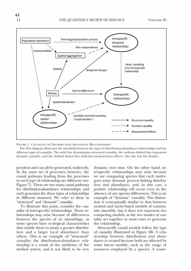
42
pendent and can all be generated, indirectly,by the same set of processes; however, thecausal pathways leading from the processesto each type of relationship are different (seeFigure 7). There are two main causal pathwaysfor distribution-abundance relationships, andeach generates the three types of relationshipsin different manners. We refer to these as“structural” and “dynamic” causality.
To illustrate this point, consider the cau-sality of interspecific relationships. These re-lationships may arise because of differencesbetween the species of an assemblage, assome species have ecological characteristicsthat enable them to attain a greater distribu-tion and a larger local abundance thanothers. This is an example of “structural”causality; the distribution-abundance rela-tionship is a result of the attributes of thestudied system, and is not likely to be very
dynamic over time. On the other hand, in-terspecific relationships may arise becausewe are comparing species that each under-goes some dynamic process linking distribu-tion and abundance, and, in this case, apositive relationship will occur even in theabsence of any species differences. This is anexample of “dynamic” causality. The distinc-tion is conceptually similar to that betweenneutral and niche-based models of commu-nity assembly, but it does not represent twocompeting models, as the two modes of cau-sality act together in most cases to generatethe relationship.
Structurally causal models follow the typeof causality illustrated in Figure 6B. A rela-tionship between distribution and abun-dance is created because both are affected bysome latent variable, such as the range ofresources employed by a species. A conse-
Figure 7. Causality of Distribution-Abundance RelationshipsThe flow diagram illustrates the interlinks between the types of distribution-abundance relationships and the
different types of causality. The solid line denominates structural causality, the uniform dashed line representsdynamic causality, and the slashed dotted line indicates measurement effects. (See the text for details.)
14 Volume 85THE QUARTERLY REVIEW OF BIOLOGY

43
quence of this is that distribution and abun-dance are not directly causally linked (i.e.,there are no arrows leading from one to theother in Figure 6B). Therefore, if the distri-bution of a species were suddenly halved byhabitat destruction, these models would notnecessarily predict any abundance changesin the remaining habitat.
Even though they are not dynamic per se,structural mechanisms will lead to temporalintraspecific relationships if the latent variable(e.g., the niche of a species) changes over time(Gaston and Lawton 1997). Such temporalchanges are predicted to move the speciesalong the regression line of the interspecificrelationship in distribution-abundance scatterplots—a pattern which has not been found inempirical studies (Webb et al. 2007). However,this is probably not a very common cause oftemporal relationships.
Dynamic causality works through a directmechanistic linkage between distributionand abundance—the type of causality illus-trated in Figure 6C. This implies that if oneof the variables changes, it will be reflectedby changes in the other; hence, distributionand abundance will track each other dynam-ically over time, although there may be a timelag in the response of one variable to the other(Gaston et al. 1999b; Conrad et al. 2001). Be-cause the distribution and abundance of thesame species are linked, the direct effect ofdynamic causality is to create intraspecific tem-poral distribution-abundance relationships. Asdescribed above, dynamic causality will alsogenerate interspecific relationships, al-though differences in the biology of spe-cies (e.g., dispersal ability) will generate“noise” and may lead to triangular relation-ships (Hartley 1998; Harte and Ostling2001).
It should be noted that the division intodynamic and structural mechanisms is notclear-cut. Metapopulation dynamics, for in-stance, have both dynamic and structuralcomponents. The basic model has dynamiccausality, as it provides a mechanistic linkagebetween the distribution and abundance ofone species: both distribution and abun-dance contribute to the number of dispers-ers in the system, and both are again affectedby the number of dispersers. But interspe-
cific differences in dispersal propensity, forexample, which may affect both distributionand abundance (Figure 6B), will contributeto interspecific relationships in a structuralmanner (this was discussed, though usingdifferent terms, in Hanski et al. 1993).
Figure 7 shows the causal linkage betweenintraspecific temporal and interspecific rela-tionships. In addition, intraspecific spatialrelationships may lead to local interspecificdistribution-abundance relationships; thisoccurs if the study area overlaps the centralpart of the range of some species, and theedges of the ranges of others (Brown 1984).This has been termed the “range position”hypothesis (Gaston and Gregory 1997) (seeTable 1), but it is not a first order biologicalmechanism in itself.
The higher empirical prevalence of inter-specific relationships (Gaston et al. 1999a)seems to indicate that structural mechanismsplay a role in the causality of distribution-abundance relationships; however, as tempo-ral relationships are regularly observed (e.g.,Borregaard and Rahbek 2006), there is alsoevidence for dynamic mechanisms. A num-ber of factors may make intraspecific rela-tionships appear weaker than they are. Forinstance, the time lag of intraspecific causal-ity tends to increase the statistical noise inrepresentations of the intraspecific distribu-tion-abundance relationship, and may pose amajor problem for the detection of patterns(Conrad et al. 2001). Furthermore, it hasbeen argued that temporal changes in thedistribution and abundance of a single spe-cies are generally of a significantly smallermagnitude than the range of values acrossthe entire assemblage, which may in itselfmake it more difficult to detect intraspecificrelationships (Gaston et al. 1999a).
A last group of mechanisms can be said tooperate within a third mode of “causality,”where distribution and abundance are notseparate entities, but merely two represen-tations of the same pattern (as argued byGregory 1998) (see Type D in Figure 6). Forexample, an interpretation of self-similaritytheory is that distribution and abundanceare just manifestations, at different scales, ofa scale-invariant clustering tendency of spe-cies distributions, measured by the fractal
March 2010 15DISTRIBUTION-ABUNDANCE RELATIONSHIPS

44
dimension (Kunin et al. 2000). This is not acausal relationship, but occurs becausedistribution and local abundance are bothmeasures of the spatial configuration of in-dividuals (see above) and, hence, are notnecessarily independent. Such nonindepen-dence between measurement of distributionand measurement of abundance may causethe observed relationship between distribu-tion and abundance to be tightly dynamic. Achange in one of the measured variables isimmediately mirrored in the measurementof the other variable. Although the consider-ation of nonindependence is conceptuallyimportant, self-similarity in itself must stillhave a cause. Thus, some other mechanism-based factor must link the distributional pat-terns of species across different spatial scales,following a straightforward Type B causality(Figure 6).
A Fresh Look at the Mechanisms:What are Distribution-AbundanceRelationships, and How Are They
Created?Hypotheses proposed to explain distribu-
tion-abundance relationships can be dividedinto groups based on their type of causality.These groups represent views describingcomplementary components of the processthat determines the distribution and abun-dance of species, and an integrated ap-proach incorporating these viewpoints isneeded to give a full picture of ecologicalcausality.
The hypotheses are formulated broadly,emphasizing general ecological structuresand dynamics while ignoring potential differ-ences between organisms. This is clearly anoversimplification. As previously noted, eachhypothesis pertains to a certain range ofscales and to certain measures of distributionand abundance, and each also reflects thebiology of the organism. For instance, meta-population dynamics are expected to occurat very different time scales for a populationof fruit flies than for forest trees. Studiesshould consider the explicit causality im-plied in relation to the temporal and spatialscale of the study, as well as how distributionand abundance were measured, and the wayin which the organism at the focus of the
study may perceive scale (Wiens 1989; Rah-bek 2005).
structural hypothesesStructural hypotheses have tended to deal
with the amount of resources available toorganisms. As originally formulated, the “re-source use” hypothesis is based on thebreadth of resource usage (Brown 1984): aspecies that can exploit a wider range of dif-ferent resources is expected to be able toexist over larger areas, and is also expectedto attain a higher density where it does oc-cur, as a greater range of resources would beavailable to the organism at any specific site.A problematic implication of this argumentis that there should be no advantage to hab-itat specialization, which can be expressed asa trade-off between high distribution andhigh local abundance. Since a specialist maybe more efficient than a generalist at exploit-ing the same resource, it may be able toattain a high abundance locally, at the cost ofa wide distribution. This implication seemsunrealistic in many cases, and there is someempirical evidence that a high degree of re-source specialization may counteract the re-source use mechanism and lead to negativedistribution-abundance relationships (seePaivinen et al. 2005 for an example amongbutterflies in Finland). In spite of this, manyauthors, somewhat misleadingly, refer to thehypothesis as the specialist-generalist hypoth-esis (e.g., Kotze et al. 2003).
Despite the intuitive appeal of the re-source hypothesis, the central assumptionthat high resource breadth should result inthe attainment of higher local abundancehas not always been empirically supported(e.g., Gregory and Gaston 2000; Kockemannet al. 2009), although several empirical stud-ies have supported this and all other keyassumptions of the hypothesis (Barger andEsch 2002; Kotze et al. 2003; Heino 2005).Breadth of resource use practically alwayscorrelates well with distribution (e.g., Har-court et al. 2005), and so claims that theresource use hypothesis can be discarded onthe basis of empirical evidence (e.g., Paivi-nen et al. 2005) seem premature.
Alternatively, a species may have more re-sources available to it if it is specialized with
16 Volume 85THE QUARTERLY REVIEW OF BIOLOGY

45
respect to a very plentiful resource. This “re-source availability” hypothesis argues thatsome species will be more widespread andabundant if the resources that they use arethemselves both widespread and abundant(Hanski et al. 1993). As the mechanism de-pends on a correlation between the distribu-tion and abundance of the resource, it hasbeen argued that this explanation merelymoves the question of causality to a lowertrophic level (Hanski et al. 1993) and, there-fore, is a secondary-level mechanism (i.e.,the distribution and abundance of the re-source still remains to be explained).
Since the distribution of resources is auto-correlated in the environment, the resource-based hypotheses are predicted to lead tointraspecific spatial distribution-abundancerelationships. The amount of suitable re-sources and habitat is predicted to be highestin an area close to the center of the range ofthe species, and to diminish away from thispoint. As the amount of resource availablecontrols both distribution and abundance, asimilar pattern is expected to appear forthese two variables, creating a spatially uni-modal relationship (Brown 1984; Brown etal. 1995).
The resource use of an organism has beeninterpreted as its “niche,” so that resourcebreadth is measured by niche width, and re-source availability by niche position (Gastonand Lawton 1997).This is convenient, sinceniche width and niche position can be quan-tified by using ordination analysis (Gregoryand Gaston 2000; e.g., Tales et al. 2004), forexample, or co-occurrence data (Fridley etal. 2007). However, care must be taken whenusing niche measures to evaluate resource-based hypotheses, as the niche encompassesboth biotic resources as well as abiotic con-ditions (Hutchinson 1957). Investigations ofthe impact of niche factors on distribution-abundance relationships should thereforeconsider the causality implied, and notmerely invoke the theory of resource avail-ability. The link between niche and distribu-tion size is straightforward (Grinnell 1917),whereas the influence of niche on abun-dance is far less clear and depends on howthe niche is defined. While the idea thatmore resources will allow a species to be-
come more abundant is not a matter of con-tention, there is no obvious link between thecommonality of a habitat—or any set of abi-otic conditions—and abundance.
Several studies have reported strong cor-relations between niche position and bothdistribution and local abundance (Gregoryand Gaston 2000; Tales et al. 2004; Heino2005). However, in these studies, niche posi-tion was based on habitat conditions at thesite where the species was found. This meansthat the resource availability mechanism, asdescribed here, cannot explain the distribu-tion-abundance correlations in these studies.Instead, studies quantifying the niche fromhabitat variables may in fact be comparingoccupancy at two scales. When the grain sizeof a study is coarser than the scale of habitatturnover, the species associated with themost sparsely distributed habitat will appearto have lesser abundance than the speciesthat are evenly distributed over the land-scape, even though the abundance withinthe species’ habitats may be the same.
In a paper entitled “Back to basics,” Holtet al. (1997) generalized the structurallycausal mechanism and integrated it with apopulation ecological perspective. Framing atheory of distribution-abundance relation-ships in terms of a simple population model,they described the limiting case in which nospatial dispersal connects the occupied sites,effectively enabling the model to ignore dy-namic processes directly linking distributionand abundance. In such a system, the relativegrowth rate r of a population is determinedby the rates of birth and death—the “vitalrates” of the population. High r leads tohigher local abundances, and, since all siteswith r � 0 are predicted to be occupied, acorrelation of abundance and distribution isexpected (Figure 6B with r as the latent vari-able), assuming that the r of populations ofthe same species are correlated (e.g., be-cause death rates are identical).
The idea is conceptually similar to Brown’sresource use hypothesis, which can be thoughtof as a special case of vital rates dynamics—thecase in which the variation in r between speciesis determined by the resource usage of thespecies. Additionally, the vital rates modelmakes explicit the required assumption that
March 2010 17DISTRIBUTION-ABUNDANCE RELATIONSHIPS

46
the strength of density-dependence is similaramong species (Holt et al. 1997). Since thevital rates model is cast explicitly in terms ofdemographic parameters, it should, at least intheory, be more amenable to empirical testing.However, very few empirical tests of this modelhave been conducted, probably because of theinherent difficulty in measuring population-level birth and death rates.
One prediction of the vital rates model isthat interspecific distribution-abundancerelationships should be shaped by the dis-tribution of habitat suitability on the land-scape and its effect on the birth rates ofpopulations. This prediction was recentlytested by Freckleton et al. (2006), in astudy that provided support for several ofthe predictions of the vital rates model.
dynamic mechanismsFor a species to be present in an area, the
presence or availability of suitable habitat andenvironment is not sufficient. The species alsohas to be able to reach the area and must besufficiently numerous (in terms of individuals)for viable population dynamics to occur (Han-ski 1999). Whereas resource-based mecha-nisms determine the distribution and size ofareas that are potentially habitable by a species,population dynamic mechanisms determinehow large a proportion of these habitable siteswill be occupied by the species at any giventime (see Figure 8 for an example).
According to the metapopulation theoryfor distribution-abundance relationships, apositive correlation between site occupancyand local population arises due to dispersalbetween patches of suitable habitat (Hanski1991a,b). The causality works in both direc-tions, and is based on the number of dispers-ing individuals in the metapopulation. Thisnumber is assumed to be a function of thenumber of occupied patches, as well as theabundance at each patch. A larger numberof dispersers will act to increase patch occu-pancy by increasing the number of coloniza-tion events, and may also serve to preventsmall subpopulations from undergoing ex-tinction (the “rescue effect”) (Hanski andGyllenberg 1993). If the level of dispersal issufficiently high compared to local popula-tion growth, immigrants may increase thelocal abundance of subpopulations by facili-tating a more rapid attainment of carryingcapacity (Hanski et al. 1993).
The metapopulation hypothesis has re-ceived some empirical support. Gonzalez et al.(1998) found that distribution-abundance re-lationships in a system of moss patches onrocks disappeared when dispersal betweenpatches was prevented, and Riis and Jensen(2002) demonstrated that aquatic plant specieswith better dispersal ability exhibited strongerrelationships between site occupancy and localabundance. However, some authors havequestioned whether most species exhibitmetapopulation dynamics at the relevanttemporal and spatial scales (e.g., Lawton1996; Newton 1997; Cowley et al. 2001).
Dynamic causality is not confined to popu-lation dynamic mechanisms. A hypothesisbased on resources was proposed by O’Connor(1987), who argued that individuals in popula-tions existing at high densities could be forcedto colonize lower quality habitats, which is ef-fectively equivalent to increasing the width ofthe realized niche. This “density-dependenthabitat selection” is expected to lead to distri-bution-abundance correlations at very localscales, although it is unlikely to result in thelinear relationships shown in Figure 3. Sincedensity is expected to be lower in the low-quality habitat, this mechanism might evenlead to a negative correlation between occu-pancy and average local density (Paivinen et al.
Figure 8. The Relationship between Structuraland Dynamic Causal Pathways
Different mechanisms affect different aspects of thedistribution of species, and may work together to createobserved patterns. Here the interaction is demonstratedfor the most commonly quoted hypotheses: the re-source use hypothesis and meta-population dynamics.
18 Volume 85THE QUARTERLY REVIEW OF BIOLOGY
47
2005). Nevertheless, this mechanism has beendemonstrated to play an important role forsome organisms, such as cod in the North At-lantic (Blanchard et al. 2005).
A hypothesis aimed at integrating theseviews was proposed by Venier and Fahrig(1996, 1998), who suggested that a synthesisbetween habitat availability and dispersal dy-namics would not have to make meta-population assumptions in order to generatedistribution-abundance relationships: If aspecies can establish and breed in a larger pro-portion of the available landscape, a largerproportion of dispersal propagules will be suc-cessful and will elevate both local abundanceand site occupancy at a landscape scale.
interspecies interactionsAt inspection, all of the proposed mecha-
nisms are found to fall within a noninteractingcommunity paradigm, in which species act outtheir population processes independently ofthe other species within the community. How-ever, species interactions are a fact of ecologi-cal reality and are repeatedly found in local aswell as individual-based studies (e.g., Brown etal. 2001; Suttle et al. 2007). In addition, thelong-lasting debate concerning whether spe-cies interactions play an important role instructuring community-level patterns nowseems to indicate that this is in fact the case(Gotelli and McCabe 2002). Processes such asinterspecific competition could certainly playan important role in structuring interspecificdistribution-abundance relationships (Holt etal. 2002b). By way of example, competitivelydominant species have been hypothesized toexpropriate portions of the potential nichespace of other species, enabling the dominantsto attain higher species densities and greatergeographical distributions (McNaughton andWolf 1970). The mechanism driving this pro-cess is basically an extension of the resourceuse hypothesis to incorporate interactions be-tween the niches of species in the community.This “competitive dominance” hypothesis isalso amenable to the critique that the effi-ciency of a species at exploiting a resource maybe related to niche breadth (as noted abovefor specialists vs. generalists); i.e., the com-petitive dominant may have a smaller niche,and hence attain a smaller spatial distribution
(the “included niche” phenomenon) (Chase1996).
Although the dispute over the influence ofinterspecific interactions on community pat-terns has persisted for more than 30 years (Di-amond 1975; Connor and Simberloff 1979;Gotelli and McCabe 2002), their potential im-portance for distribution-abundance relation-ships has been addressed by few studies. Instudies of microcosms, Holt et al. (2002b) dem-onstrated that communities where severalspecies were allowed to interact did, in fact,generate stronger distribution-abundance rela-tionships than noninteracting communities.While these results are promising, microcosmsare different from natural systems (Rick-lefs 2004), and we have yet to see any fieldstudies demonstrating the role of interspecificinteractions.
Distribution-AbundanceRelationships as Spatial Aggregation
Based on an argument by Wright (1991), adifferent school of thought maintains thatdistribution-abundance relationships aremerely the result of the clumped nature ofthe spatial distribution of organisms (Hartley1998; Holt et al. 2002a). To understand this,one can consider two extreme cases for aspecies increasing its population size: (1) ifnew individuals never occupy the same site asexisting individuals, the number of occupiedsites will increase linearly with populationsize, and (2) if new individuals always settlein already occupied sites, the local abun-dance will increase linearly with populationsize. For any case between those two ex-tremes, both the number of occupied sitesand the local abundance will increase whenpopulation size increases (Figure 6B).
Accordingly, even if the individuals of aspecies are randomly distributed, a positivedistribution-abundance relationship can beexpected (Wright 1991). This suggests that aPoisson distribution is a more correct null hy-pothesis for testing distribution-abundance re-lationships than the flat baseline assumption ofno relationship that is used in most studies(Hartley 1998; for a discussion of null models,see Gotelli and Graves 1996). However, the useof a Poisson-based baseline has not, somewhat
March 2010 19DISTRIBUTION-ABUNDANCE RELATIONSHIPS
48
surprisingly, been generally implemented (butsee Falster et al. 2001; Conlisk et al 2009).
Regressions of observed values of localabundance on distribution size are steeperthan those predicted by the Poisson distribu-tion (Wright 1991). However, the distribu-tion of most organisms is not random butrather exhibits some degree of spatial aggre-gation, which may be modeled as a negativebinomial (or similar) distribution (Hartley1998; He et al. 2002). Using realistic values forthe aggregation parameter in these distribu-tions renders a good fit with observed distribu-tion-abundance relationships (Hartley 1998).
Modeling aggregation patterns of individ-uals usually assumes rather small spatial ex-tents (e.g. Hartley 1998) in which the habitatis relatively homogenous; however, there isno reason why aggregation at higher levelscould not also be described by models ofindividual aggregation (hence the dottedline in Figure 4).
A different way of expressing aggregation inspecies’ distributions is described by the self-similarity theory. Whereas the individual aggre-gation theory models the structure of speciesdistributions at larger scales from very local-scale, individual locations, the self-similaritytheory takes a top-down approach and useslarge-scale distribution patterns to model ag-gregation at smaller scales (Kunin et al. 2000).The basis for this model is an observationthat many natural patterns have a similarstructure regardless of spatial scale; i.e., theyhave fractal properties (Halley et al. 2004).The distribution of the individuals of a spe-cies is one measure that has been shown tobe self-similar over a certain range of scales(Ostling et al. 2000). Models incorporatingthis species-level self-similarity consistentlygenerate a positive relationship between oc-cupancy and local abundance (Harte andOstling 2001).
Since self-similarity theory makes explicitmathematical predictions about the relation-ship between distribution and abundance, anumber of studies have attempted to use it toestimate abundance directly based on thedensity of occupied sites at larger scales. Thestudies carried out so far have yielded somepromising results (Hui and McGeoch 2007;Conlisk et al 2009), with potential applica-
tion for conservation-orientated monitoringprograms (Kunin 1998; He and Gaston2000a; Figueiredo and Grelle 2009).
The main theoretical difficulty associatedwith the application of the self-similarityhypothesis to distribution-abundance rela-tionships is that it is not clear whether theself-similarity condition should be assumedto apply to the distribution of individuals ofone species (species-level self-similarity), orto the distribution of the species within acommunity (community-level self-similarity)(Harte et al. 1999; Ostling et al. 2000). Thesetwo types of self-similarity are mutually exclu-sive unless the fractal dimensions of all spe-cies are identical (Green et al. 2003), andonly species-level similarity is expected tolead to realistic distribution-abundancerelationships (Harte and Ostling 2001).However, it has been suggested that the ho-mogenizing effect of factors such as geomet-ric constraints and the distribution of habitaton the fractal dimension of species couldreconcile these theories (Sizling and Storch2004).
Recently, Storch and colleagues imple-mented the general concept of aggregation asa determinant of most macroecological pat-terns in a framework based on the idea of“general fractals” (Storch et al. 2008). By sub-dividing patches into random sub-patches atconsecutive, discrete levels of spatial scale in asimulation model, they were able to generateseveral empirically established macroecologicalpatterns, including species-area relationshipsand realistic abundance frequency distribu-tions. They also suggested that the distribution-abundance relationship might be explained bythis framework. This work further strengthensthe argument for an aggregation-based causal-ity for distribution-abundance relationships.
It has been repeatedly argued that theconcept of spatial aggregation is merely away of rephrasing distribution-abundance re-lationships in terms of a different patternand is, thus, of limited value (Gaston et al.1998b; Paivinen et al. 2005; Blackburn et al.2006). However, synonymizing separate pat-terns and combining the theory surroundingthem is in itself a worthwhile goal of theoret-ical science (Lakatos 1978). Furthermore, itshould not be overlooked that if distribution-
20 Volume 85THE QUARTERLY REVIEW OF BIOLOGY

49
abundance relationships are merely anotherexpression of aggregation across spatialscales, this will significantly increase the num-ber of potential mechanisms and change ourview of their causality. Any behavioral or eco-logical process that acts to increase aggregation(e.g., limitations on juvenile dispersal, flockingbehavior, and habitat requirements) will thenplay a role in generating distribution-abundance relationships.
This accounts for the appearance of distri-bution-abundance relationships in the neu-tral model of biodiversity (Hubbell 2001). Inneutral models, distribution-abundance rela-tionships appear as a result of the spatialstructure of colonization and dispersal onthe community grid (Bell 2000, 2001). Thesefactors act to produce positive relationshipsthrough their combined effect on the spatialaggregation of individuals, as dispersers origi-nate from a few colonized spots and move onlya limited distance before settling (Bell 2001).
Not only does spatial aggregation underliethe distribution-abundance relationships gen-erated by these “unifying theories” of macro-ecology (Harte et al. 1999; Bell 2001; McGilland Collins 2003; Storch et al. 2008), but, asdescribed in the section on structural mecha-nisms, it may also be the factor driving theeffect of niche characteristics on relationshipsbetween distribution and abundance, as habi-tat specificity creates aggregation.
A Tentative SynthesisHave all the pieces of the puzzle regarding
the causality of distribution-abundance rela-tionships fallen into place? Not quite yet. Butthe scale-specific causal framework outlinedin this paper indicates how the complete pic-ture may appear.
Distribution-abundance relationships occuras a complex interplay of ecosystem structuralfactors and the dynamics of individual popula-tions (Figure 7). The different habitat and re-source requirements of organisms mean thateach species perceives the landscape in a spe-cific manner. Species with abundantly availableresources have dense distributions and attaingreater local abundances, resulting in positiveinterspecific distribution-abundance relation-ships. Within that context, population dy-namics link the occupancy of habitat patches
with local abundances of each species dy-namically, creating consistent relationshipsacross time (temporal intraspecific relation-ships). These two pathways are not sharply de-limited, and they affect each other mutually.Since interspecific relationships are compari-sons of species that each experience popula-tion dynamics, these relationships are alsoaffected by dispersal-based mechanisms, al-though the effect may be obscured by speciesdifferences. Similarly, since the resource basisfor species varies in time and space, both tem-poral and local spatial relationships of the dis-tribution and abundance of individual specieswill be created by the structural causal pathway.
This entire system describes a series of pro-cesses that causally link distribution andabundance as though they were two separatemeasures. However, it is questionablewhether they can be treated like completelyindependent entities. The spatial clusteringwill affect measures of both distribution andabundance for each species, further contrib-uting to linking the two variables. This non-causal link has very different properties fromthe mechanistic hypotheses, as it is primarilyan effect of how distribution and abundanceare measured and defined. Importantly, thisview of distribution-abundance relationshipsallows for a much wider range of potentialecological explanations. However, the de-gree to which distribution and abundanceare mechanistically linked or merely linkedthrough aggregation remains a largely unre-solved question that should be a priority forfuture investigations. This can only be inves-tigated, most likely, through controlledexperiments specifically targeted at the indi-vidual hypotheses. The few experimentalstudies that have been conducted thus farseem to indicate that a mechanistic causalityplays at least some role in generating thevarious forms of distribution-abundance re-lationships (e.g., Gonzalez et al. 1998).
acknowledgments
The authors thank the Danish National Research Foun-dation for its support of the Center for Macroecology,Evolution and Climate. We also thank Dr. Robert Holtand an anonymous reviewer for insightful commentsand constructive criticism of the manuscript, which sig-nificantly improved the final version.
March 2010 21DISTRIBUTION-ABUNDANCE RELATIONSHIPS

50
REFERENCES
Andrewartha H. G., Birch L. C. 1954. The Distributionand Abundance of Animals. Chicago (IL): Universityof Chicago Press.
Balmford A., Bond W. 2005. Trends in the state ofnature and their implications for human well-being. Ecology Letters 8(11):1218–1234.
Barger M. A., Esch G. W. 2002. Host specificity and thedistribution-abundance relationship in a communityof parasites infecting fishes in streams of NorthCarolina. Journal of Parasitology 88(3):446–453.
Bell G. 2000. The distribution of abundance in neu-tral communities. American Naturalist 155(5): 606–617.
Bell G. 2001. Neutral macroecology. Science 293(5539):2413–2418.
Bibby C. J., Burgess N. D., Hill D. A. 1992. Bird CensusTechniques. London (UK): Academic Press.
Blackburn T. M., Cassey P., Gaston K. J. 2006. Varia-tions on a theme: sources of heterogeneity in theform of the interspecific relationship betweenabundance and distribution. Journal of Animal Ecol-ogy 75(6):1426–1439.
Blackburn T. M., Gaston K. J., Quinn R. M., Arnold H.,Gregory R. D. 1997. Of mice and wrens: the relationbetween abundance and geographic range size inBritish mammals and birds. Philosophical Transactionsof the Royal Society of London, Series B: Biological Sciences352(1352):419–427.
Blanchard J. L., Mills C., Jennings S., Fox C. J., Rack-ham B. D., Eastwood P. D., O’Brien C. M. 2005.Distribution-abundance relationships for NorthSea Atlantic cod (Gadus morhua): observation ver-sus theory. Canadian Journal of Fisheries and AquaticSciences 62(9):2001–2009.
Bock C. E. 1987. Distribution-abundance relation-ships of some Arizona landbirds: a matter of scale.Ecology 68(1):124–129.
Bock C. E., Ricklefs R. E. 1983. Range size and localabundance of some North American songbirds: apositive correlation. American Naturalist 122:295–299.
Borregaard M. K., Rahbek C. 2006. Prevalence ofintraspecific relationships between range size andabundance in Danish birds. Diversity and Distribu-tions 12(4):417–422.
Brown J. H. 1984. On the relationship between abun-dance and distribution of species. American Natu-ralist 124:255–279.
Brown J. H., Maurer B. A. 1987. Evolution of speciesassemblages: effects of energetic constraints and spe-cies dynamics on the diversification of the NorthAmerican avifauna. American Naturalist 130:1–17.
Brown J. H., Maurer B. A. 1989. Macroecology: thedivision of food and space among species on con-tinents. Science 243(4895):1145–1150.
Brown J. H., Mehlman D. W., Stevens G. C. 1995. Spatialvariation in abundance. Ecology 76(7):2028–2043.
Brown J. H., Stevens G. C., Kaufman D. M. 1996. Thegeographic range: size, shape, boundaries, andinternal structure. Annual Review of Ecology andSystematics 27:597–623.
Brown J. H., Whitham T. G., Morgan Ernest S. K.,Gehring C. A. 2001. Complex species interactionsand the dynamics of ecological systems: long-termexperiments. Science 293(5530):643–650.
Chamberlain T. C. 1890. The method of multipleworking hypotheses. Science 15:92–96.
Chase J. M. 1996. Differential competitive interac-tions and the included niche: an experimentalanalysis with grasshoppers. Oikos 76:103–112.
Chust G., Pretus J. L., Ducrot D., Bedos A., DeharvengL. 2003. Identification of landscape units from aninsect perspective. Ecography 26(3):257–268.
Collins S. L., Glenn S. M. 1997. Effects of organismaland distance scaling on analysis of species distribu-tion and abundance. Ecological Applications 7:543–551.
Colwell R. K., Rahbek C., Gotelli N. J. 2004. Themid-domain effect and species richness patterns:what have we learned so far? American Naturalist163:E1–E23.
Conlisk E., Conlisk J., Enquist B., Thompson J., HarteJ. 2009. Improved abundance prediction frompresence-absence data. Global Ecology and Biogeog-raphy 18(1):1–10.
Connor E. F., Simberloff D. 1979. The assembly ofspecies communities: chance or competition? Ecol-ogy 60(6):1132–1140.
Conrad K. F., Perry J. N., Woiwod I. P. 2001. Anabundance-occupancy time-lag during the declineof an arctiid tiger moth. Ecology Letters 4(4):300–303.
Cowley M. J. R., Thomas C. D., Wilson R. J., Leon-Cortes J. L., Gutierrez D., Bulman C. R. 2001.Density-distribution relationships in British butter-flies. II. An assessment of mechanisms. Journal ofAnimal Ecology 70(3):426–441.
Currie D. J., Mittelbach G. G., Cornell H. V., Field R.,Guegan J. F., Hawkins B. A., Kaufman D. M., KerrJ. T., Oberdorff T., O’Brien E. M., Turner J. R. G.2004. Predictions and tests of climate-based hy-potheses of broad-scale variation in taxonomicrichness. Ecology Letters 7(12):1121–1134.
Diamond J. M. 1975. Assembly of species communi-ties. Pages 342–444 in Ecology and Evolution of Com-munities, edited by M. L. Cody and J. M. Diamond.Cambridge (MA): Harvard University Press.
Falster D. S., Murray B. R., Lepschi B. J. 2001. Linkingabundance, occupancy and spatial structure: anempirical test of a neutral model in an open-forest
22 Volume 85THE QUARTERLY REVIEW OF BIOLOGY

51
woody plant community in eastern Australia. Jour-nal of Biogeography 28(3):317–323.
Figueiredo M. S. L., Grelle C. E. V. 2009. Predictingglobal abundance of a threatened species from itsoccurrence: implications for conservation plan-ning. Diversity and Distributions 15(1):117–121.
Foggo A., Frost M. T., Attrill M. J. 2003. Abundance-occupancy patterns in British estuarine macroinver-tebrates. Marine Ecology Progress Series 265:297–302.
Freckleton R. P., Noble D., Webb T. J. 2006. Distribu-tions of habitat suitability and the abundance-occupancy relationship. American Naturalist 167:260–275.
Fridley J. D., Vandermast D. B., Kuppinger D. M., Man-they M. I. C. H., Peet R. K. 2007. Co-occurrencebased assessment of habitat generalists and special-ists: a new approach for the measurement of nichewidth. Journal of Ecology 95(4):707–722.
Frost M. T., Attrill M. J., Rowden A. A., Foggo A. 2004.Abundance-occupancy relationships in macro-fauna on exposed sandy beaches: patterns andmechanisms. Ecography 27(5):643–649.
Gaston K. J. 1994. Rarity. London (UK): Chapmanand Hall.
Gaston K J. 1996. The multiple forms of the interspecificabundance-distribution relationship. Oikos 76:211–220.
Gaston K. J. 1998. Ecology: rarity as double jeopardy.Nature 394(6690):229–230.
Gaston K. J. 1999. Implications of interspecific andintraspecific abundance-occupancy relationships.Oikos 86:195–207.
Gaston K. J., Blackburn T. M. 2003. Dispersal and theinterspecific abundance-occupancy relationshipin British birds. Global Ecology and Biogeography12(5):373–379.
Gaston K. J., Blackburn T. M., Gregory R. D. 1998a. Inter-specific differences in intraspecific abundance-rangesize relationships of British breeding birds. Ecography21(2):149–158.
Gaston K. J., Blackburn T. M., Gregory R. D. 1999a.Intraspecific abundance-occupancy relationships:case studies of six bird species in Britain. Diversityand Distributions 5(5):197–212.
Gaston K. J., Blackburn T. M., Lawton J. H. 1997.Interspecific abundance range size relationships:an appraisal of mechanisms. Journal of Animal Ecol-ogy 66(4):579–601.
Gaston K. J., Blackburn T. M., Lawton J. H. 1998b. Aggre-gation and interspecific abundance-occupancy rela-tionships. Journal of Animal Ecology 67:995–999.
Gaston K. J., Greenwood J. J. D., Gregory R. D., QuinnR. M., Lawton J. H. 2000. Abundance-occupancyrelationships. Journal of Applied Ecology 37:39–59.
Gaston K. J., Gregory R. D. 1997. Interspecific abundance-range size relationships: range position and phylog-eny. Ecography 20:390–399.
Gaston K. J., Gregory R. D., Blackburn T. M. 1999b.Intraspecific relationships between abundanceand occupancy among species of Paridae and Syl-viidae in Britain. Ecoscience 6:131–142.
Gaston K. J., Gregory R. D., Greenwood J. J. D. 1998c.The anatomy of the interspecific abundance-range size relationship for the British avifauna. I.Spatial patterns. Ecology Letters 1(1):38–46.
Gaston K. J., Lawton J. H. 1990. Effects of scale andhabitat on the relationship between regional dis-tribution and local abundance. Oikos 58:329–335.
Gonzalez A., Lawton J. H., Gilbert F. S., BlackburnT. M., Evans-Freke I. 1998. Metapopulation dy-namics, abundance, and distribution in a micro-ecosystem. Science 281(5385):2045–2047.
Gotelli N. J., Graves G. R. 1996. Null Models in Ecology.Washington (D.C.): Smithsonian Institution Press.
Gotelli N. J., McCabe D. J. 2002. Species co-occur-rence: a meta-analysis of J. M. Diamond’s assemblyrules model. Ecology 83(8):2091–2096.
Green J. L., Harte J., Ostling A. 2003. Species rich-ness, endemism and abundance patterns: tests oftwo fractal models in a serpentine grassland. Ecol-ogy Letters 6:919–928.
Gregory R. D. 1995. Phylogeny and relations amongabundance, geographical range and body-size ofBritish breeding birds. Philosophical Transactions ofthe Royal Society of London, Series B: Biological Sciences349(1330):345–351.
Gregory R. D. 1998. An intraspecific model of species’expansion, linking abundance and distribution.Ecography 21(1):92–96.
Gregory R. D., Gaston K. J. 2000. Explanations ofcommonness and rarity in British breeding birds:separating resource use and resource availability.Oikos 88(3):515–526.
Grell M. B. 1998. Fuglenes Danmark. Copenhagen (Den-mark): Gads Forlag.
Grinnell J. 1917. Field tests of theories concerningdistributional control. American Naturalist 51(602):115–128.
Guo Q., Brown J. H., Valone T. J. 2000. Abundanceand distribution of desert annuals: are spatial andtemporal patterns related? Journal of Ecology 88(4):551–560.
Halley J. M., Hartley S., Kallimanis A. S., Kunin W. E.,Lennon J. J., Sgardelis S. P. 2004. Uses and abusesof fractal method in ecology. Ecology Letters 7(3):254–271.
Hanski I. 1991a. Reply to Nee, Gregory and May. Oikos62:88–89.
Hanski I. 1991b. Single-species metapopulation dy-namics: concepts, models and observations. Biolog-ical Journal of the Linnean Society 42:17–38.
Hanski I. 1999. Metapopulation Ecology. Oxford (UK):Oxford University Press.
Hanski I., Gyllenberg M. 1993. Two general meta-
March 2010 23DISTRIBUTION-ABUNDANCE RELATIONSHIPS

52
population models and the core-satellite specieshypothesis. American Naturalist 142:17–41.
Hanski I, Gyllenberg M. 1997. Uniting two generalpatterns in the distribution of species. Science275(5298):397–400.
Hanski I., Kouki J., Halkka A. 1993. Three explana-tions of the positive relationship between distribu-tion and abundance of species. Pages 108–116 inSpecies Diversity in Ecological Communities: Historicaland Geographical Perspectives, edited by R. E. Rick-lefs and D. Schluter. Chicago (IL): University ofChicago Press.
Harcourt A. H., Coppeto S. A., Parks S. A. 2005. Thedistribution-abundance (density) relationship: itsform and causes in a tropical mammal order, Pri-mates. Journal of Biogeography 32(4):565–579.
Harte J., Kinzig A., Green J. L. 1999. Self-similarity inthe distribution and abundance of species. Science284(5412):334–336.
Harte J., Ostling A. 2001. Self-similarity and the rela-tionship between abundance and range size. Amer-ican Naturalist 157:374–386.
Hartley S. 1998. A positive relationship between localabundance and regional occupancy is almost in-evitable (but not all positive relationships are thesame). Journal of Animal Ecology 67(6):992–994.
Hartley S., Kunin W. E. 2003. Scale dependency ofrarity, extinction risk, and conservation priority.Conservation Biology 17(6):1559–1570.
Harvey P. H., Pagel M. 1991. The Comparative Method inEvolutionary Biology. Oxford (UK): Oxford Univer-sity Press.
He F. L., Gaston K. J. 2000a. Estimating species abun-dance from occurrence. American Naturalist 156:553–559.
He F. L., Gaston K. J. 2000b. Occupancy-abundancerelationships and sampling scales. Ecography 23:503–511.
He F. L., Gaston K. J., Wu J. G. 2002. On speciesoccupancy-abundance models. Ecoscience 9:119–126.
Heino J. 2005. Positive relationship between regionaldistribution and local abundance in stream in-sects: a consequence of niche breadth or nicheposition? Ecography 28:345–354.
Holt A. R., Gaston K. J. 2003. Interspecific abundance-occupancy relationships of British mammals and birds:is it possible to explain the residual variation? GlobalEcology and Biogeography 12:37–46.
Holt A. R., Gaston K. J., He F. L. 2002a. Occupancy-abundance relationships and spatial distribution:a review. Basic and Applied Ecology 3:1–13.
Holt A. R., Warren P. H., Gaston K. J. 2002b. Theimportance of biotic interactions in abundance-occupancy relationships. Journal of Animal Ecology71:846–854.
Holt R. D., Lawton J. H., Gaston K. J., Blackburn T. M.
1997. On the relationship between range size andlocal abundance: back to basics. Oikos 78:183–190.
Hubbell S. P. 2001. The Unified Neutral Theory of Biodi-versity and Biogeography. Princeton (NJ): PrincetonUniversity Press.
Hui C., McGeoch M. A. 2007. Capturing the “droopy-tail” in the occupancy-abundance relationship.Ecoscience 14(1):103–108.
Hurlbert A. H., White E. P. 2005. Disparity betweenrange map- and survey-based analyses of speciesrichness: patterns, processes and implications.Ecology Letters 8:319–327.
Hutchinson G. E. 1957. Concluding remarks. ColdSpring Harbour Symposium on Quantitative Biology22:415–427.
Jetz W., Wilcove D. S., Dobson A. P. 2007. Projectedimpacts of climate and land-use change on theglobal diversity of birds. PLoS Biology 5(6):e157.
Johnson C. N. 1998. Species extinction and the rela-tionship between distribution and abundance. Na-ture 394(6690):272–274.
Kockemann B., Buschmann H., Leuschner C. 2009.The relationship between abundance, range sizeand niche breadth in Central European tree spe-cies. Journal of Biogeography 36:854–864.
Kotze D. J., Niemela J., O’Hara R. B., Turin H. 2003.Testing abundance-range size relationships in Eu-ropean carabid beetles (Coleoptera, Carabidae).Ecography 26:553–566.
Kunin W. E. 1998. Extrapolating species abundanceacross spatial scales. Science 281(5382):1513–1515.
Kunin W. E., Hartley S., Lennon J. J. 2000. Scalingdown: on the challenge of estimating abundancefrom occurrence patterns. American Naturalist 156:560–566.
Lacy R. C., Bock C. E. 1986. The correlation betweenrange size and local abundance of some NorthAmerican birds. Ecology 67:258–260.
Lakatos I. 1978. Philosophical Papers. Cambridge (UK):Cambridge University Press.
Lawton J. H. 1996. Population abundances, geo-graphic ranges and conservation: 1994 WitherbyLecture. Bird Study 43:3–19.
Leibold M. A., Holyoak M., Mouquet N., AmarasekareP., Chase J. M., Hoopes M. F., Holt R. D., ShurinJ. B., Law R., Tilman D., Loreau M., Gonzalez A.2004. The metacommunity concept: a frameworkfor multi-scale community ecology. Ecology Letters7:601–613.
Lyons S. K., Willig M. R. 2002. Species richness, lati-tude, and scale-sensitivity. Ecology 83:47–58.
McGill B., Collins C. 2003. A unified theory for mac-roecology based on spatial patterns of abundance.Evolutionary Ecology Research 5:469–492.
McGill B. J., Etienne R. S., Gray J. S., Alonso D., Ander-son M. J., Benecha H. K., Dornelas M., Enquist B. J.,Green J. L., He F., Hurlbert A. H., Magurran A. E.,
24 Volume 85THE QUARTERLY REVIEW OF BIOLOGY
53
Marquet P. A., Maurer B. A., Ostling A., SoykanC. U., Ugland K. I., White E. P. 2007. Species abun-dance distributions: moving beyond single predic-tion theories to integration within an ecologicalframework. Ecology Letters 10:995–1015.
McNaughton S. J., Wolf L. L. 1970. Dominance andthe niche in ecological systems. Science 167(3915):131–139.
Nee S., Gregory R. D., May R. M. 1991. Core and satellitespecies: theory and artefacts. Oikos 62:83–87.
Newton I. 1997. Links between the abundance anddistribution of birds. Ecography 20:137–145.
Novotny V. 1991. Effect of habitat persistence on therelationship between geographic-distribution andlocal abundance. Oikos 61:431–433.
O’Connor R. J. 1987. Organization of avian assem-blages: the influence of intraspecific habitatdynamics. Pages 163–183 in Organization of Com-munities: Past and Present, edited by J. H. R. Geeand P. S. Giller. Oxford (UK): Blackwell ScientificPublications.
Ostling A., Harte J., Green J. L., Condit R. 2000.Self-similarity and clustering in the spatial distri-bution of species. Science 290:671a.
Paivinen J., Grapputo A., Kaitala V., Komonen A.,Kotiaho J. S., Saarinen K., Wahlberg N. 2005. Neg-ative density-distribution relationship in butter-flies. BMC Biology 3:5.
Pollard E., Moss D., Yates T. J. 1995. Populationtrends of common British butterflies at monitoredsites. Journal of Applied Ecology 32:9–16.
Rahbek C. 2005. The role of spatial scale and theperception of large-scale species-richness patterns.Ecology Letters 8:224–239.
Rahbek C., Graves G. R. 2001. Multiscale assessmentof patterns of avian species richness. Proceedings ofthe National Academy of Sciences USA 98:4534–4539.
Reif J., Horak D., Sedlacek O., Riegert J., Pesata M.,Hrazsky Z., Janecek S., Storch D. 2006. Unusualabundance-range size relationship in an Afromon-tane bird community: the effect of geographicalisolation? Journal of Biogeography 11:1959–1968.
Ricklefs R. E. 2004. A comprehensive framework for globalpatterns in biodiversity. Ecology Letters 7:1–15.
Riis T., Sand-Jensen K. 2002. Abundance-range sizerelationships in stream vegetation in Denmark.Plant Ecology 161(2):175–183.
Rosenzweig M. L. 1995. Species Diversity in Space and Time.Cambridge (UK): Cambridge University Press.
Scheiner S. M., Cox S. B., Willig M. R., MittelbachG. G., Osenberg C., Kaspari M. 2000. Species rich-ness, species-area curves, and Simpson’s paradox.Evolutionary Ecology Research 2:791–802.
Selmi S., Boulinier T. 2004. Distribution-abundancerelationship for passerines breeding in Tunisianoases: test of the sampling hypothesis. Oecologia139:440–445.
Shipley B. 2004. Cause and Correlation in Biology: AUser’s Guide to Path Analysis, Structural Equationsand Causal Inference. Cambridge (UK) and NewYork: Cambridge University Press.
Sizling A. L., Storch D. 2004. Power-law species-arearelationships and self-similar species distributionswithin finite areas. Ecology Letters 7:60–68.
Storch D., Sizling A. L., Reif J., Polechova J., Sizlin-gova E., Gaston K. J. 2008. The quest for a nullmodel for macroecological patterns: geometry ofspecies distributions at multiple spatial scales. Ecol-ogy Letters 11:771–784.
Suttle K. B., Thomsen M. A., Power M. E. 2007. Spe-cies interactions reverse grassland responses tochanging climate. Science 315:640–642.
Symonds M. R. E., Johnson C. N. 2006. Range size-abundance relationships in Australian passerines.Global Ecology and Biogeography 15:143–152.
Tales E., Keith P., Oberdorff T. 2004. Density-rangesize relationships in French riverine fishes. Oecolo-gia 138:360–370.
Thompson K., Hodgson J. G., Gaston K. J. 1998.Abundance-range size relationships in the herba-ceous flora of central England. Journal of Ecology86:439–448.
Venier L. A., Fahrig L. 1996. Habitat availability causes thespecies abundance-distribution relationship. Oikos 76:564–570.
Venier L. A., Fahrig L. 1998. Intra-specific abundance-distribution relationships. Oikos 82:483–490.
Webb T. J., Noble D., Freckleton R. P. 2007. Abundance-occupancy dynamics in a human dominated envi-ronment: linking interspecific and intraspecifictrends in British farmland and woodland birds.Journal of Animal Ecology 76(1):123–134.
Whittaker R. J. 1965. Dominance and diversity in landplant communities. Science 147:250–259.
Wiens J. A. 1989. Spatial scaling in ecology. FunctionalEcology 3:385–397.
Williamson M., Gaston K. J. 1999. A simple transforma-tion for sets of range sizes. Ecography 22:674–680.
Willig M. R., Kaufman D. M., Stevens R. D. 2003.Latitudinal gradients of biodiversity: pattern, pro-cess, scale, and synthesis. Annual Review of Ecology,Evolution, and Systematics 34:273.
Wilson P. D. 2008. The pervasive influence of samplingand methodological artefacts on a macroecologi-cal pattern: the abundance-occupancy relation-ship. Global Ecology and Biogeography 17:457–464.
Wright D. H. 1991. Correlations between incidenceand abundance are expected by chance. Journal ofBiogeography 18:463–466.
Zuckerberg B., Porter W. F., Corwin K. 2009. Theconsistency and stability of abundance-occupancyrelationships in large-scale population dynamics.Journal of Animal Ecology 78(1):172–181.
Associate Editor: Monica G. Turner
March 2010 25DISTRIBUTION-ABUNDANCE RELATIONSHIPS


Unpublished Manuscript
Chapter 2:Are species-range distributions
consistent with range-size heritability?

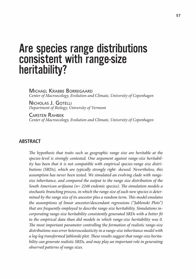
57
Are species range distributions consistent with range-size heritability?
Michael KraBBe BorregaardCenter of Macroecology, Evolution and Climate, University of Copenhagen
Nicholas J. gotelliDepartment of Biology, University of Vermont
carsteN rahBeKCenter of Macroecology, Evolution and Climate, University of Copenhagen
ABSTRACT
The hypothesis that traits such as geographic range size are heritable at the species-level is strongly contested. One argument against range-size heritabil-ity has been that it is not compatible with empirical species-range size distri-butions (SRDs), which are typically strongly right- skewed. Nevertheless, this assumption has never been tested. We simulated an evolving clade with range-size inheritance, and compared the output to the range size distribution of the South American avifauna (n= 2248 endemic species). The simulation models a stochastic branching process, in which the range size of each new species is deter-mined by the range size of its ancestor plus a random term. This model emulates the assumptions of linear ancestor/descendant regressions (“Jablonski Plots”) that are frequently employed to describe range-size heritability. Simulations in-corporating range-size heritability consistently generated SRDs with a better fit to the empirical data than did models in which range-size heritability was 0. The most important parameter controlling the formation of realistic range-size distributions was error heteroscedasticity in a range-size inheritance model with a log-log transformed Jablonski plot. These results suggest that range-size herita-bility can generate realistic SRDs, and may play an important role in generating observed patterns of range sizes.

58585858
INTRODUCTION
The existence of species-level heritability of species traits, such as geographic range size, is hotly contested. The notion of heritability is central to evolution: A certain proportion of the variance in a trait is passed on from parents to descendants, es-tablishing the basis for selective pressures to lead to trait evolution (Huxley 1942). Whereas this is basic knowledge at the level of individual organisms, some authors have also suggested that the notion of heritability could be transferred to other lev-els of organization, e.g. to the species level (Lewontin 1970; Stanley 1975; Jablonski 1987).This would create a theoretical basis for higher-level selection regimes, such as selection at the species level (for discussions of hierarchical selection models, see Rice 1995; Diniz-Filho 2004; Jablonski 2007).
Species-level traits can be divided into ‘aggregate’ and ‘emergent’ traits (Diniz-Filho 2004). Aggregate traits are traits such as body size, which is merely a statistical aggregate of the sizes of individuals. These traits are not expected to be affected by higher-level selection, because individual-level selection processes occur faster, and thus overwhelm any species-level effects (Williams 1966). Emergent traits, on the other hand, are traits existing only at the species level. Probably the clearest example of such an emergent trait is species range size (Diniz-Filho 2004; Jablonski 2007). Thus, most of the discussion of species-level heritability has concerned heritability of range sizes (Jablonski 1987; Webb & Gaston 2003; Hunt et al. 2005; Webb & Gaston 2005; Mouillot & Gaston 2007; Waldron 2007).
Importantly, ‘heritability’ at the level of individuals and species are not identi-cal concepts. When diploid individuals reproduce, the meiotic event transfers ge-netic material directly from parents to offspring. The genetic material then interacts with the environment to shape the phenotypical trait. The strength of this interaction determines the level of heritability, which can be estimated by the slope of a linear regression between the trait values of offspring and parents. In species-level herit-ability, the process of speciation is viewed as an analogue to the reproductive events of individuals. Species-level heritability thus refers to a relationship between the trait of a species, and the trait of its ancestor on the phylogenetic tree (Jablonski 1987).
Such relationships could occur if ancestors and descendants share some trait that predisposes them to attain a large distribution, such as dispersal ability (Bohning-Gaese et al. 2006; van Bocxlaer et al. 2010). Ancestors and descendants are also likely to have similar environmental niches (Peterson et al. 1999), and thus be confined to the same habitats (Mouillot & Gaston 2009). These putative causes of species-level heritability are similar to the cause of individual-level heritability, which is that par-ents and offspring share genes that predispose them for e.g. a certain body size.
However, the parallel is not absolute. In a speciation event, the original species ceases to exist (by definition); the disparate populations comprising the original spe-cies then constitute two new species (Mayr 1963). These two species occupy parts
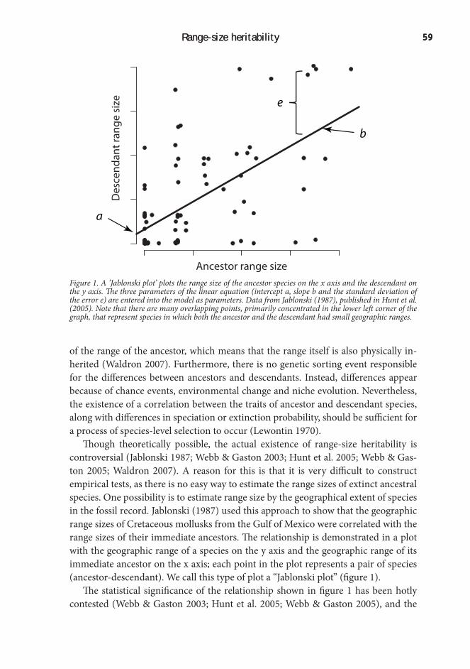
59Range-size heritability 59Range-size heritability
Ancestor range size
Des
cend
ant r
ange
siz
e
b
a
e
Figure 1. A ’Jablonski plot’ plots the range size of the ancestor species on the x axis and the descendant on the y axis. The three parameters of the linear equation (intercept a, slope b and the standard deviation of the error e) are entered into the model as parameters. Data from Jablonski (1987), published in Hunt et al. (2005). Note that there are many overlapping points, primarily concentrated in the lower left corner of the graph, that represent species in which both the ancestor and the descendant had small geographic ranges.
of the range of the ancestor, which means that the range itself is also physically in-herited (Waldron 2007). Furthermore, there is no genetic sorting event responsible for the differences between ancestors and descendants. Instead, differences appear because of chance events, environmental change and niche evolution. Nevertheless, the existence of a correlation between the traits of ancestor and descendant species, along with differences in speciation or extinction probability, should be sufficient for a process of species-level selection to occur (Lewontin 1970).
Though theoretically possible, the actual existence of range-size heritability is controversial (Jablonski 1987; Webb & Gaston 2003; Hunt et al. 2005; Webb & Gas-ton 2005; Waldron 2007). A reason for this is that it is very difficult to construct empirical tests, as there is no easy way to estimate the range sizes of extinct ancestral species. One possibility is to estimate range size by the geographical extent of species in the fossil record. Jablonski (1987) used this approach to show that the geographic range sizes of Cretaceous mollusks from the Gulf of Mexico were correlated with the range sizes of their immediate ancestors. The relationship is demonstrated in a plot with the geographic range of a species on the y axis and the geographic range of its immediate ancestor on the x axis; each point in the plot represents a pair of species (ancestor-descendant). We call this type of plot a “Jablonski plot” (figure 1).
The statistical significance of the relationship shown in figure 1 has been hotly contested (Webb & Gaston 2003; Hunt et al. 2005; Webb & Gaston 2005), and the

6060
analysis has never been repeated because of the lack of suitable fossil data. An al-ternative approach was suggested by Webb and Gaston (2003), who proposed that if range sizes were heritable, the range sizes of extant sister species should be more symmetrical than expected by chance. They defined a measure of asymmetry as the ratio of the smaller to the larger range size of sister species. Such an approach poten-tially offers important advantages, as it does not require fossil data and thus could be applied to the many data sets of extant species. For a clade of 103 sister species pairs of birds, Webb and Gaston (2003) showed that empirical range size asymmetries were not different from those expected from a null model.
Webb and Gaston’s (2003) test of range-size asymmetry has been critiqued on two fronts. Waldron (2007) objected that the physical division of the ancestor range at speciation would tend to make range sizes of sister species asymmetrical rather than symmetrical, thus invalidating the null model of Webb and Gaston (2003). Hunt et al. (2005) also criticized the null model of Webb and Gaston (2003), as assumes that the species-range size (SRD) of the organisms is uniform. Applying a null model based on the empirical SRD instead supported the interpretation of range size heritability. Webb and Gaston (2005) countered that Hunt et al.’s (2005) use of the empirical SRD is potentially circular: If range sizes are heritable, this itself would affect the SRD of assemblages. They write:
“Results [of modeling range size heritability] can also be applied to more general questions regarding the species–range size distribution; for instance, What form would the species–range size distribution take if range sizes were heritable? or, equivalently, Is the form and phylogenetic structure of the species–range size dis-tribution compatible with a scenario of range size heritability? The answer to this second question would generally appear to be no.”
Here, we address the latter question. Although Webb and Gaston (2005) maintain that the answer would generally appear to be no, they offer no further arguments in support of this claim. Whereas the second part of the question, concerning the phy-logenetic signal in range sizes, has been addressed by several authors (e.g. Freckleton et al. 2002; Jones et al. 2005), this study is the first to address the form of the species-range size distribution.
To evaluate the effects of range size heritability on the shape of SRDs, we con-structed a relatively simple stochastic branching model of speciation and extinction, and incorporated varying degrees of range-size heritability. We calibrated the model with data on the SRD of the extant South American avifauna and used the model results to address two questions: 1) If range sizes are heritable, what patterns would be expected to arise in a Jablonski plot of ancestral and descendant ranges? 2) Can a model of range-size heritability generate a SRD that resembles empirical data for extant assemblages?

61Range-size heritability
X
Figure 2. The range size of each species is determined by a branching process of speciation and extinction. Lineage termination (at point X) occurs with a probability that is inversely proportional to range size. The sizes of the ovals shown are generated with the assumption of log axis scaling on the Jablonski plot.
MATERIALS.AND.METHODS
We used a computer simulation approach to investigate the impact of range-size her-itability on the frequency distribution of range sizes. The simulation is based on a simple branching process of speciation, in which the range size of each new spe-cies is determined by that of its immediate ancestor (Figures 1 and 2). In nature, the range sizes of species undergo anagenetic changes over their lifetimes (Liow & Stenseth 2007), but we restricted ourselves to model the range size change during cladogenesis, similar to how individual-level heritability is measured. Although our model thus does not include all of the details of range size dynamics, it does provide a parsimonious representation of the effect of range size inheritance on the range size frequency distribution.
Domain.Size.and.Assemblage.Size
Our simulation is not spatially explicit in that we did not model the placement or location of species ranges in a geographic domain (Jetz & Rahbek 2001; Colwell et al. 2004). However, we do assume that species ranges are represented as occurrences in a

6262
domain of similar-sized grid cells. Within such a domain, we are modeling the range extent at a large spatial scale.
To evaluate the model, we compared its predictions to a high-quality empirical data set on the range sizes of the South American avifauna (Graves & Rahbek 2005). The domain size was set at 1689, which is the number of 1° x 1° grid cells encompass-ing the continent of South America. The number of extant species generated in a sin-gle run of the simulation was set at 2869, which is the number of endemic breeding species in South America whose geographic ranges are entirely contained within the continent (Rahbek et al. 2007). Preliminary analyses indicated that simulating addi-tional species did not change the shape of the SRD: Post hoc inspection showed that most simulations had reached a stable average range size by the end of the simulation.
The.Inheritance.of.Geographic.Range.Size
The simulation begins with a single ancestor species, with a given range size s, that will give rise to all the extant species at the end of the simulation. At each time step, each species in the assemblage may go extinct with a probability E. Each surviving species may then speciate with a probability S, thereby adding a new species to the as-semblage. Thus, multiple speciation and extinction events are possible within a single time step, although extinction always precedes speciation within a time step. The core of the simulation is the equation determining the range size of descendant species: the range size of the descendant species is a linear function of the range size of the ancestor species (see figure 1).
where D is the domain size (1689), desc and anc are the range sizes of the descendant and ancestor, and the slope (b), intercept (a) and error term (e) are model param-eters that are varied over a full factorial lattice design. This model corresponds to the empirical Jablonski plots (Jablonski 1987), in which geographic ranges of ancestor and descendant species are plotted on the x and y axes and fit with a simple linear regression.
The heritability function was calculated on either linear or logarithmic axes of range size. Plotting the equation on a log-log scale is equivalent to assuming a non-linear power function for the relationship between ancestor and descendant range size:
In Jablonski’s (1987) original paper, ‘range size’ referred to the linear one-dimen-sional extent of mollusk ranges measured along the Gulf of Mexico and the Atlantic coastal plain of North America. When applying this analysis to the two-dimensional ranges of many terrestrial organisms, a linear extent in one dimension scales with the
,desc aD b anc N eD0)= + + ^ h
( ) ( ) ( ) , (ln ln ln lndesc a D b anc N e D0) ) )= + + ^ h

63Range-size heritability
square root of the range’s total two-dimensional area. Hence, a linear measure would be roughly approximated as a plot of range areas on log-transformed axes. The choice between log and linear axes has important implications for the error term. An error term that is constant in log space will increase with the predicted value when back-transformed into linear space. This means that the variability will be greater for large range sizes.
Out-of-bounds.rule
When the stochastic range generated by the heritability equation falls outside the bounds of the geographic domain (i.e. smaller than 1 grid cell or larger than the size of the domain) it cannot be used as a descendant range. We tried two algorithms for correcting out-of-bound ranges : (1) The range is discarded, and a new value gener-ated, until a permissible range size is attained (truncation); (2) the new range size is set to 1 grid cell if it is too small or is set to the domain size if it is too large (absorbing boundaries). Both of these algorithms potentially alter the linearity of the ancestor-descendant relation, and the effects will be more extreme as more out-of-bounds range sizes are generated.
Likelihood.of.speciation.and.extinction
It is debated whether the probability of speciation is affected be range size, and there are empirical examples of both positive (Mouillot & Gaston 2007) and negative (Ja-blonski & Roy 2003) correlations between range size and speciation probability. To model positive correlations, we set the probability of speciation in one time step for each species as: range size / domain size * 0.01. To model negative correlations, we set the probability of speciation in one time step for each species as (1 - range size / domain size) * 0.01. Under a model of no relationship, we set the probability of spe-ciation as 0.01 for all species in each time step, regardless of their range sizes.
Extinction probability, on the other hand, is unambiguously related to range size: small ranging species are far more likely to go extinct than widespread species (McKinney 1997; McKinney & Lockwood 1999). The extinction probability in each time step was calculated as (1 – range size / domain size) * 0.005, where the constant 0.005 was chosen to ensure that speciation events outnumbered extinction events. Hence, species numbers grew throughout the simulation, from 1 ancestral species at the start of the simulation to the pre-established bound of 2248 extant descendant species at the end. To ensure that most simulations did not end with extinction of the entire assemblage, each simulation was preceded by a short burn-in period so that no extinctions were allowed until the assemblage contained at least 20 species.

6464
Mode.of.Speciation
The simulation implemented two speciation mechanisms: ‘range splitting’ and ‘found-er event’ speciation (Waldron 2007). Range splitting speciation models a vicariance event that splits a species into two isolated populations (Mayr 1963). Founder event speciation models a new species as a population that buds off the range of an existing species, e.g., as in an island-mainland scenario. Range splitting speciation was im-plemented by removing the ancestor species and adding two descendants with range sizes generated from the Jablonski model (figure 1). In founder-event speciation, one of the descendants retained the range size of the ancestor. We also implemented a ‘mixed’ scenario, where 50% of speciation events were of each type (determined ran-domly).
Empirical.data
The correspondence of the simulated SRD to the empirical data was quantified by calculating the χ2 deviation statistic on the rank-ordered sizes of the ranges of South American birds and the sizes of the rank-ordered simulated ranges. This is calculated as
where n is the number of species (2869), emp and sim are the empirical and simu-lated range-size distributions, and i refers to any particular rank (e.g., the smallest or largest range size of each distribution) (Gotelli & Ellison 2004). Empirical range size frequency distributions are typically very right-skewed, with only a small number of species having large ranges. We log-transformed range sizes before comparison be-cause we did not want the test to be overly weighted by the large frequency classes of small-ranged species. Log-transformed distributions often were approximately nor-mal, which gave more even weight to patterns in all of the range size classes than did the untransformed data (Graves & Rahbek 2005).
Lattice.structure
The entire model encompassed a set of four parameters with discrete values: Jablon-ski plot axis (linear, log), speciation mode (range splitting, founder event, mixed), boundary conditions (absorbing, truncating), speciation likelihood (proportional, inverse, constant); and three continuous parameters for range-size heritability: slope, intercept, and error variance (range of parameter values in Table 1).
To evaluate the effect of these parameters on the SRD, we ran the simulation for all different combinations of the parameters in a full lattice design, and compared the resulting SRD to the empirical data. The simulation was run twice to save computer time: In an initial run, all combinations of the categorical values were explored. In a subsequent run, the best fitting categorical parameter combinations were employed
( )emp
sim empX
i
i i
i
i n2
2
1
=-
=
=
/
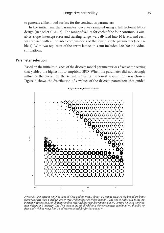
65Range-size heritability
Figure A1. For certain combinations of slope and intercept, almost all ranges violated the boundary limits (range size less than 1 grid square or greater than the size of the domain). The size of each circle is the pro-portion of species in a simulation run that exceeded the boundary limits, out of 300 runs for each combina-tion of slope and intercept. The clear area in the middle delimits those parameter combinations that did not frequently violate range limits and were retained for further analyses.
to generate a likelihood surface for the continuous parameters.In the initial run, the parameter space was sampled using a full factorial lattice
design (Rangel et al. 2007). The range of values for each of the four continuous vari-ables, slope, intercept error and starting range, were divided into 10 levels, and each was crossed with all possible combinations of the four discrete parameters (see Ta-ble 1). With two replicates of the entire lattice, this run included 720,000 individual simulations.
Parameter.selection
Based on the initial run, each of the discrete model parameters was fixed at the setting that yielded the highest fit to empirical SRD. When the parameter did not strongly influence the overall fit, the setting requiring the fewest assumptions was chosen. Figure 3 shows the distribution of χ2values of the discrete parameters that guided

6666
Figure 3. The influence of the static parameter assumptions on the fit (measured as the χ2 difference) of simulated to empirical RSFDs. Each panel gives the Tukey box plots for all 720,000 simulations in the initial model, partitioned by the discrete parameter settings. The box encompasses 50% of the distribution, the horizontal bar is the median, and the whiskers identify the largest (or smallest) non-outlier point. A low value indicates a good fit. A. The type of speciation. B. The relationship between range size and speciation likelihood. C. The scaling of the Jablonski plot axes. D. The action taken when a projected range is smaller than 1 or larger than the size of the domain. On all plots, the 5% significance level of 2358 (χ2 deviance on 2247 df) is indicated by a horizontal dashed line.
this selection.Simulation output was analyzed and visualized in R (R 2009). All simulations
were implemented in C++, compiling with MinGW gcc within the Code::Blocks open source IDE (http://www.codeblocks.org/).

67Range-size heritability
χ2
Freq
uenc
y
0 5000 10000 15000
020
0040
0060
0080
00
Figure 4. The distribution of fit values generated by the fine-grained second simulation. With 2247 d.f., the 0.05 significance level of the χ2 distribution is ≈2358 (indicated by the dashed line). 43% of the models in the second simulation showed an adequate fit with the empirical data (p > 0.05).
RESULTS
Discrete.parameter.selection
Seventy-eight percent of the simulations in the initial run went to completion within 5000 time steps. Of 720,000 simulations of the initial run, 58,140 (8%) of the simu-lated assemblages went extinct before reaching 2689 species, and 106,572 (14%) did not reach 2689 species within 5000 time steps (figure A1). These represented mainly non-viable parameter combinations: Altering these numbers by changing speciation and extinction likelihoods did not affect any of the results below.
Some parameter combinations led to impermissible ranges being generated, i.e. negative ranges or ranges higher than the domain size (figure A1). The range sizes of these species could still be incorporated according to the boundary procedure, but high numbers of impermissible ranges meant that the slope and intercept value de-fined a line outside the reasonable parameter space (i.e. parts of the line went outside the plotting region in figure 1). Instead of determining these from the outset, we ran the simulation for all combinations of slope and intercept, and then excluded the simulations for which more than 10% of the ranges had been affected by the bound-
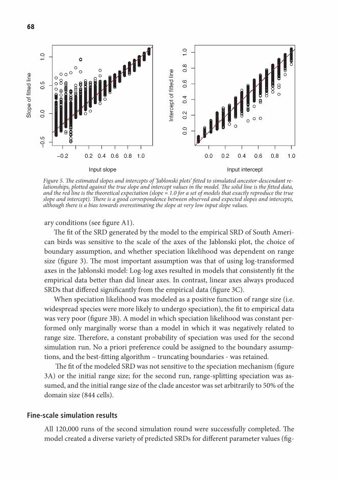
6868
Figure 5. The estimated slopes and intercepts of ‘Jablonski plots’ fitted to simulated ancestor-descendant re-lationships, plotted against the true slope and intercept values in the model. The solid line is the fitted data, and the red line is the theoretical expectation (slope = 1.0 for a set of models that exactly reproduce the true slope and intercept). There is a good correspondence between observed and expected slopes and intercepts, although there is a bias towards overestimating the slope at very low input slope values.
ary conditions (see figure A1).The fit of the SRD generated by the model to the empirical SRD of South Ameri-
can birds was sensitive to the scale of the axes of the Jablonski plot, the choice of boundary assumption, and whether speciation likelihood was dependent on range size (figure 3). The most important assumption was that of using log-transformed axes in the Jablonski model: Log-log axes resulted in models that consistently fit the empirical data better than did linear axes. In contrast, linear axes always produced SRDs that differed significantly from the empirical data (figure 3C).
When speciation likelihood was modeled as a positive function of range size (i.e. widespread species were more likely to undergo speciation), the fit to empirical data was very poor (figure 3B). A model in which speciation likelihood was constant per-formed only marginally worse than a model in which it was negatively related to range size. Therefore, a constant probability of speciation was used for the second simulation run. No a priori preference could be assigned to the boundary assump-tions, and the best-fitting algorithm – truncating boundaries - was retained.
The fit of the modeled SRD was not sensitive to the speciation mechanism (figure 3A) or the initial range size; for the second run, range-splitting speciation was as-sumed, and the initial range size of the clade ancestor was set arbitrarily to 50% of the domain size (844 cells).
Fine-scale.simulation.results
All 120,000 runs of the second simulation round were successfully completed. The model created a diverse variety of predicted SRDs for different parameter values (fig-

69Range-size heritability
Slope
Inte
rcep
t
−0.3 −0.075 0.15 0.3 0.45 0.6 0.75 0.9 1.05
−0.1
250.
10.
250.
40.
550.
70.
851
540
690
882
1126
1439
1839
2358
3001
3834
4899
6259
7997
10218
13054
16679
χ2
Figure 6. The fit of the model RSFD as a function of input slope and intercept values. The color scaling is based on log-transformed χ2 deviance values. Dark blue indicates the best fit, dark red indicate the poorest fit, with green and yellow indicating an intermediate fit. The bluish colors symbolize χ2 deviance values that are not significant at the 0.05 level assuming 2247 d.f., i.e. less than 2358 (indicated in bold on the legend). The black dot with cross hairs indicates the mean and 95% confidence intervals of the slope and intercept es-timates from the gastropod data of Jablonski (1987; reanalysis of the dataset published by Hunt et al 2005).
ure A2). However, 43% of the simulations generated a SRD that fit the empirical data well (p > 0.05, see figure 4). The goodness-of-fit (measured as the χ2 deviance) was positively correlated with the scatter parameter e, indicating that the process error of the Jablonski model played an important role in generating realistic range-size distri-butions. The relationship was monotonic over the range of parameters we modeled: a larger error term generally led to more realistic distributions. This indicates that the relationship between the error term and range size, created by using log axes in the Jablonski model, was a main driver of the model fit.
Post hoc regressions of simulated descendant and ancestor range sizes performed reasonably well at estimating the true slope and intercept (figure 5). This result sug-gests that simple Jablonski plots are a reasonable method for estimating range-size heritability. However, when the slope was close to zero, there was a bias towards over-estimating the slope in Jablonski plots (figure 5, left panel).
A small set of parameter combinations produced SRD’s that were statistically in-distinguishable from empirical patterns (figure 6). The ridge of light-blue shading in Figure 6 indicates that realistic SRDs can be generated over a range of moderate to

7070
steep slope values. A scenario of no heritability is equivalent to a slope of 0 in figure 6. The SRD generated using a slope of 0 is a log-normal distribution, which fits reason-ably well when the intercept equals the geometric mean of the empirical range sizes. However, the empirical SRD is more strongly right-skewed than a log-normal dis-tribution, and the best fit was obtained with a model in which range-size heritability had a steep slope of ~1 (darkest blue squares in figure 6). The heritability estimates from Jablonski’s gastropod data, when mapped on this parameter space, would gen-erate an SRD that fits the avian data more poorly (green shading).
DISCUSSION
The main result of our simulation analyses is that a simple evolutionary model can generate a realistic SRD, with characteristic right hand skew and a predominance of small-ranged species. Contrary to previous predictions, incorporating range-size heritability in the model led to a better fit with the SRD of the South American avi-fauna. The best fit was found with a model in which the heritability slope was steep (about 1.0; Figure 6), whereas a model with no heritability resulted in a log-normal distribution which fit the empirical data more poorly. Although these results do not conclusively demonstrate that range-size heritability occurs in nature, they do coun-ter Webb and Gaston’s (2005) claim that observed SRDs are incompatible with the hierarchical branching processes of an evolving clade.
When Jablonski’s estimated heritability values for gastropods are plotted on the simulation parameter space (figure 6), they fall within the favorable zone of param-eter values, although not in the region where the fit is best. We would not expect the fit to be perfect: the continental range sizes of extant birds are controlled by different processes than gastropod ranges inferred from fossil data. In addition, Jablonski’s (1987) analysis may underestimate the degree of heritability, due to unclarities in the phylogenetic relationship of species and incomplete sampling of the fossil strata.
A problematic assumption of the simulation model is that species ranges are mod-eled as a single value, though range sizes may change dramatically over evolutionary time (Liow & Stenseth 2007). The simulated range size may be interpreted as range-size ‘tendency’, or alternatively the mean range size of a species over its evolutionary lifetime. However, we cannot assume that the ranges of South American birds are all equivalent to the species’ mean lifetime range. The problem is related to determining heritability in the body size of constantly growing organisms, such as trees. This can be done by comparing size/time growth curves; unfortunately, such curves are not feasible to create for range sizes. Nevertheless, the high similarity of SRDs for differ-ent organism groups (Gaston 1996) implies that dynamical processes of range size changes do not markedly change the shape of range distributions.
The issue of range size heritability forces us to rethink our approach to macroevo-

71Range-size heritability
loutionary studies. Phylogenetic comparative methods are limited by the complica-tion that ranges are inherited in two different ways: indirectly, because ancestor and descendant species share ecological traits, and directly, because the physical range of the ancestor is shared by the descendants at the speciation event (Waldron 2007). These two types make contrasting predictions about the ranges of sister species. As we do not know the relative strengths of these two types of heritability, the method of sister species comparisons (e.g. Webb & Gaston 2003; Webb & Gaston 2005) is not reliable.
An innovative solution to this was suggested by Waldron (Waldron 2007), who used an explicit model of range division to generate an expected distribution of the symmetry of sister species’ range sizes, and compared this to the empirically observed pattern. The analysis showed that sister species were actually more symmetrical than expected from direct range inheritance, thus to some degree supporting the assump-tion of range-size heritability. However, this kind of null model only considers direct inheritance. In addition, it models only the terminal branching event, and thus does not emulate the patterns generated in a stochastic branching model of speciation and extinction.
Though challenging, the problem of multiple mechanisms of heritability is not unique to species-level heritability. Indeed, traditional heritability also results from mixed causality - including numerous forms of maternal and environmental effects, epistasis, and complex interactions between genes, environment, and phenotype (Futuyma 1998). Nevertheless, the large temporal scale involved in species-level processes limits the amount of data that may become available to bear on this issue, which means that simulation-based approaches like the one used here and in Wal-dron (Waldron 2007) is likely to play a major role in this field.
The observation that a simple function of range-size heritability can generate a realistic SRD is in itself an important result, because the causes of the strong right skew of empirical range distributions are not very well understood (Gaston 1996). In our model, the right skew of the SRD appears to result from variance heteroscedas-ticity in the descendant range size generated by the log-log transformation of the Jablonski plot: the descendant of a wide-ranging species might inherit either a large or a small geographic range, whereas the descendant of a small-ranging species is usually constrained to inherit a small geographic range. As a consequence, phyloge-netic lineages in the model that start out with small range sizes tend to pass that trait on to their descendants. Large-ranged species would tend to produce large-ranged descendants, but would also sometimes produce a descendant with a small range. As a consequence, with the passage of evolutionary time, many species with small ranges are generated, but relatively few species with large ranges are generated. Thus, range size inheritance combined with stochastic speciation and extinction in an evolving lineage is a simple mechanistic process that could account for the predominance of relatively small-ranged species in most empirical assemblages.
7272
ACKNOWLEDGEMENTS:
We thank Gary Graves and David Jablonski for comments on the manuscript. CR and MKB thank the Danish National Research Foundation for its support of the Center for Macroecology, Evolution and Climate. NJG was supported by the U.S. National Science Foundation (NSF DEB-0541936) and the Department of Energy (DOE DE-FG02-08ER64510).
REFERENCES:
van Bocxlaer I., Loader S.P., Roelants K., Biju S.D., Menegon M. & Bossuyt F. (2010). Gradual Adaptation Toward a Range-Expansion Phenotype Initiated the Global Radiation of Toads. Science, 327, 679-682.
Bohning-Gaese K., Caprano T., van Ewijk K. & Veith M. (2006). Range size: Disentangling cur-rent traits and phylogenetic and biogeographic factors. American Naturalist, 167, 555-567.
Colwell R.K., Rahbek C. & Gotelli N.J. (2004). The mid-domain effect and species richness pat-terns: What have we learned so far? American Naturalist.
Diniz-Filho J.A.F. (2004). Macroecology and the hierarchical expansion of evolutionary theory. Global Ecology and Biogeography, 13, 1-5.
Freckleton R.P., Harvey P.H. & Pagel M. (2002). Phylogenetic analysis and comparative data: A test and review of evidence. American Naturalist, 160, 712-726.
Futuyma D.J. (1998). Evolutionary Biology. Sinauer Associates, Inc., Sunderland, Massachu-setts.
Gaston K.J. (1996). Species-range-size distributions: Patterns, mechanisms and implications. Trends in Ecology & Evolution, 11, 197-201.
Gotelli N.J. & Ellison A.M. (2004). A primer of ecological statistics. Sinauer Associates, Inc., Sunderland, Massachusetts.
Graves G.R. & Rahbek C. (2005). Source pool geometry and the assembly of continental avifau-nas. Proceedings of the National Academy of Sciences, 102, 7871-7876.
Hunt G., Roy K. & Jablonski D. (2005). Species-Level Heritability Reaffirmed: A Comment on “On the Heritability of Geographic Range Sizes”. The American Naturalist, 166, 129-135.
Huxley J. (1942). Evolution: The Modern Synthesis. Allen & Unwin, London.
Jablonski D. (2007). Scale and hierarchy in macroevolution. Palaeontology, 50, 87-109.
Jablonski D. & Roy K. (2003). Geographical range and speciation in fossil and living molluscs. Proceedings of the Royal Society of London Series B-Biological Sciences, 270, 401-406.
Jablonski D.A.V.I. (1987). Heritability at the Species Level: Analysis of Geographic Ranges of Cretaceous Mollusks. Science, 238, 360-363.
Jetz W. & Rahbek C. (2001). Geometric constraints explain much of the species richness pattern

73Range-size heritability
in African birds. Proceedings of the National Academy of Sciences of the United States of America, 98, 5661-5666.
Jones K.E., Sechrest W. & Gittleman J.L. (2005). Age and area revisited: identifying global pat-terns and implications for conservation. In: Phylogeny and conservation (eds. Purvis A, Gittleman JL & Brooks TM). Cambridge University Press Cambridge, pp. 141-165.
Lewontin R.C. (1970). The Units of Selection. Annual Review of Ecology and Systematics, 1, 1-18.
Liow L.H. & Stenseth N.C. (2007). The rise and fall of species: implications for macroevolution-ary and macroecological studies. Proceedings of the Royal Society B: Biological Sciences, 274, 2745-2752.
Mayr E. (1963). Animal species and evolution. Harvard University Press, Boston, Massachu-setts.
McKinney M.L. (1997). Extinction vulnerability and selectivity: Combining ecological and pa-leontological views. Annual Review of Ecology and Systematics, 28, 495-516.
McKinney M.L. & Lockwood J.L. (1999). Biotic homogenization: a few winners replacing many losers in the next mass extinction. Trends in Ecology & Evolution, 14, 450-453.
Mouillot D. & Gaston K. (2009). Spatial overlap enhances geographic range size conservatism. Ecography, 32, 671-675.
Mouillot D. & Gaston K.J. (2007). Geographical range size heritability: what do neutral models with different modes of speciation predict? Global Ecology and Biogeography, 16, 367-380.
Peterson A.T., Sober¢n J. & S nchez-Cordero V. (1999). Conservatism of Ecological Niches in Evolutionary Time. Science, 285, 1265-1267.
R D.C.T. (2009). R: A language and environment for statistical computing. In. R Foundation for Statistical Computing Vienna, Austria.
Rahbek C., Gotelli N.J., Colwell R.K., Entsminger G.L., Rangel T.F.L.V. & Graves G.R. (2007). Predicting continental-scale patterns of bird species richness with spatially explicit models. Proceedings of the Royal Society B-Biological Sciences, 274, 165-174.
Rangel T.F.L.V., Diniz-Filho J.A.F. & Colwell R.K. (2007). Species richness and evolutionary niche dynamics: A spatial pattern-oriented simulation experiment. American Naturalist, 170, 602-616.
Rice S.H. (1995). A genetical theory of species selection. Journal of Theoretical Biology, 177, 237-245.
Stanley S.M. (1975). A theory of evolution above the species level. Proceedings of the National Academy of Sciences, 72, 646-650.
Waldron A. (2007). Null models of geographic range size evolution reaffirm its heritability. American Naturalist, 170, 221-231.
Webb T.J. & Gaston K.J. (2003). On the heritability of geographic range sizes. American Natu-ralist, 161, 553-566.
Webb T.J. & Gaston K.J. (2005). Heritability of Geographic Range Sizes Revisited: A Reply to Hunt et al. The American Naturalist, 166, 136-143.
Williams G.C. (1966). Adaptation and natural selection. Princeton University Press, Princeton,

NJ.

Published as:Borregaard, M. K. and Rahbek, C. 2010. Dispersion fields,
diversity fields and null models: Uniting range sizes and species richness. Ecography Early View.
Chapter 3:Dispersion fields, diversity fields and null models: uniting range sizes and
species richness

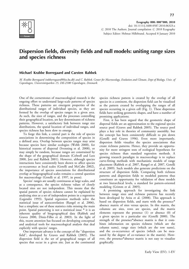
77
Dispersion fields, diversity fields and null models: uniting range sizesand species richness
Michael Krabbe Borregaard and Carsten Rahbek
M. Krabbe Borregaard ([email protected]) and C. Rahbek, Center for Macroecology, Evolution and Climate, Dept of Biology, Univ. ofCopenhagen, Universitetsparken 15, DK-2100 Copenhagen, Denmark.
One of the cornerstones of macroecological research is theongoing effort to understand large-scale patterns of speciesrichness. These patterns are emergent properties of thedistributional ranges of individual species, as they areformed by the overlap of species ranges in a given area.As such, the sizes of ranges, and the processes controllingtheir geographical location, are key determinants of richnesspatterns. However, a satisfactory link between range sizedistributions, the spatial location of individual ranges, andspecies richness has been slow to emerge.
To forge this link, a central part is the role of speciesassociations in determining the composition of species ina defined area. Overlap between species ranges may arisebecause species have similar ecologies (Webb 2000), forhistorical reasons of dispersal (Svenning et al. 2008), ormay simply be random, because ranges are constrained bythe shape of the geographical domain (Colwell and Lees2000, Jetz and Rahbek 2001). However, although speciesinteractions have consistently been shown to affect speciesco-occurrence at local scales (Gotelli and McCabe 2002),the importance of species associations for distributionaloverlap at biogeographical scales remains a central questionfor macroecology (Gotelli et al. 1997, in press).
Species’ ranges are usually continuous at large scales, andas a consequence, the species richness values of closelylocated sites are not independent. This means that thespatial pattern of species richness cannot be explained byanalyzing sites as a set of independent points in a regression(Legendre 1993). Spatial regression methods solve thestatistical issue of autocorrelation (Rangel et al. 2006),but a simplistic use of these statistics risks missing the mainpoint. Spatial patterning is not a statistical issue � it is aninherent quality of biogeographical data (Rahbek andGraves 2000, Diniz-Filho et al. 2003). In the light ofthis, recent attention has focused on developing conceptualand analytical tools for macroecological analysis that dealexplicitly with species’ ranges.
One important advance is the concept of the ‘‘dispersionfield’’, developed by Graves and Rahbek (2005). Thedispersion field is the set of geographical ranges of allspecies that occur in a given site. Just as the continental
species richness pattern is created by the overlap of allspecies in a continent, the dispersion field can be visualizedas the pattern created by overlapping the ranges of allspecies occurring in a given cell (Fig. 1). These dispersionfields have striking geometric shapes, and have a number ofpromising applications.
First, it has been argued that the geometric shape ofdispersal fields are an approximation to the regional speciessource pool (Graves and Rahbek 2005). The source poolplays a key role in theories of community assembly, butthe concept has been consistently difficult to pin down(Gotelli and Graves 1996). Even more importantly,dispersion fields visualize the species associations thatcreate richness patterns. Hence, they provide an opportu-nity for more stringent tests of ecological hypotheses forspecies richness than standard regression methods. Agrowing research paradigm in macroecology is to replacecurve-fitting methods with mechanistic models of rangeplacement (Rahbek et al. 2007, Rangel et al. 2007, Gotelliet al. 2009). Such models also generate predictions on thestructure of dispersion fields. Comparing both richnesspatterns and dispersion fields to modeled patterns thusconstitutes an opportunity for validation of these modelsat two hierarchical levels, a standard for pattern-orientedmodeling (Grimm et al. 2005).
A promising approach for investigating the linkbetween range sizes and richness patterns has recentlybeen developed by Arita et al. (2008). This approach isbased on dispersion fields, and starts with the presence�absence matrix of sites versus species. In this matrix, thecolumns are sites, rows are species, and the matrixelements represent the presence (1) or absence (0) ofa given species in a particular site (Gotelli 2000). Thestrength of the presence�absence matrix is that it com-bines information on species richness (which are thecolumn sums), range sizes (which are the row sums),and the co-occurrence of species (which can be mea-sured by the degree of co-variance in the matrix). How-ever, the presence�absence matrix is not easy to visualizegraphically.
Ecography 000: 000�000, 2010doi: 10.1111/j.1600-0587.2010.06323.x
# 2010 The Authors. Journal compilation # 2010 Ecography
Subject Editor: Helmut Hillebrand. Accepted 8 January 2010
Early View (EV): 1-EV
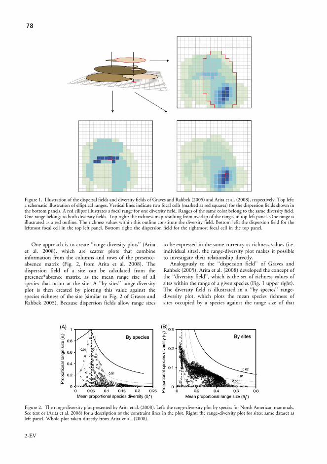
78
One approach is to create ‘‘range-diversity plots’’ (Aritaet al. 2008), which are scatter plots that combineinformation from the columns and rows of the presence-absence matrix (Fig. 2, from Arita et al. 2008). Thedispersion field of a site can be calculated from thepresence�absence matrix, as the mean range size of allspecies that occur at the site. A ‘‘by sites’’ range-diversityplot is then created by plotting this value against thespecies richness of the site (similar to Fig. 2 of Graves andRahbek 2005). Because dispersion fields allow range sizes
to be expressed in the same currency as richness values (i.e.individual sites), the range-diversity plot makes it possibleto investigate their relationship directly.
Analogously to the ‘‘dispersion field’’ of Graves andRahbek (2005), Arita et al. (2008) developed the concept ofthe ‘‘diversity field’’, which is the set of richness values ofsites within the range of a given species (Fig. 1 upper right).The diversity field is illustrated in a ‘‘by species’’ range-diversity plot, which plots the mean species richness ofsites occupied by a species against the range size of that
Figure 1. Illustration of the dispersal fields and diversity fields of Graves and Rahbek (2005) and Arita et al. (2008), respectively. Top left:a schematic illustration of elliptical ranges. Vertical lines indicate two focal cells (marked as red squares) for the dispersion fields shown inthe bottom panels. A red ellipse illustrates a focal range for one diversity field. Ranges of the same color belong to the same diversity field.One range belongs to both diversity fields. Top right: the richness map resulting from overlap of the ranges in top left panel. One range isillustrated as a red outline. The richness values within this outline constitute the diversity field. Bottom left: the dispersion field for theleftmost focal cell in the top left panel. Bottom right: the dispersion field for the rightmost focal cell in the top panel.
Figure 2. The range-diversity plot presented by Arita et al. (2008). Left: the range-diversity plot by species for North American mammals.See text or (Arita et al. 2008) for a description of the constraint lines in the plot. Right: the range-diversity plot for sites; same dataset asleft panel. Whole plot taken directly from Arita et al. (2008).
2-EV
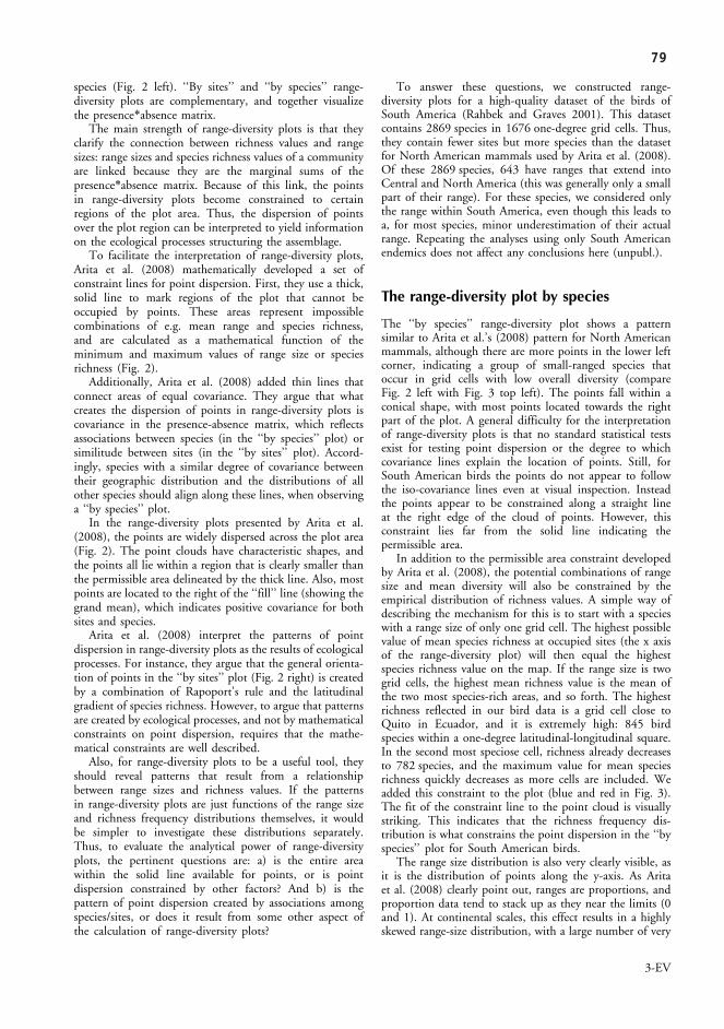
79
species (Fig. 2 left). ‘‘By sites’’ and ‘‘by species’’ range-diversity plots are complementary, and together visualizethe presence�absence matrix.
The main strength of range-diversity plots is that theyclarify the connection between richness values and rangesizes: range sizes and species richness values of a communityare linked because they are the marginal sums of thepresence�absence matrix. Because of this link, the pointsin range-diversity plots become constrained to certainregions of the plot area. Thus, the dispersion of pointsover the plot region can be interpreted to yield informationon the ecological processes structuring the assemblage.
To facilitate the interpretation of range-diversity plots,Arita et al. (2008) mathematically developed a set ofconstraint lines for point dispersion. First, they use a thick,solid line to mark regions of the plot that cannot beoccupied by points. These areas represent impossiblecombinations of e.g. mean range and species richness,and are calculated as a mathematical function of theminimum and maximum values of range size or speciesrichness (Fig. 2).
Additionally, Arita et al. (2008) added thin lines thatconnect areas of equal covariance. They argue that whatcreates the dispersion of points in range-diversity plots iscovariance in the presence-absence matrix, which reflectsassociations between species (in the ‘‘by species’’ plot) orsimilitude between sites (in the ‘‘by sites’’ plot). Accord-ingly, species with a similar degree of covariance betweentheir geographic distribution and the distributions of allother species should align along these lines, when observinga ‘‘by species’’ plot.
In the range-diversity plots presented by Arita et al.(2008), the points are widely dispersed across the plot area(Fig. 2). The point clouds have characteristic shapes, andthe points all lie within a region that is clearly smaller thanthe permissible area delineated by the thick line. Also, mostpoints are located to the right of the ‘‘fill’’ line (showing thegrand mean), which indicates positive covariance for bothsites and species.
Arita et al. (2008) interpret the patterns of pointdispersion in range-diversity plots as the results of ecologicalprocesses. For instance, they argue that the general orienta-tion of points in the ‘‘by sites’’ plot (Fig. 2 right) is createdby a combination of Rapoport’s rule and the latitudinalgradient of species richness. However, to argue that patternsare created by ecological processes, and not by mathematicalconstraints on point dispersion, requires that the mathe-matical constraints are well described.
Also, for range-diversity plots to be a useful tool, theyshould reveal patterns that result from a relationshipbetween range sizes and richness values. If the patternsin range-diversity plots are just functions of the range sizeand richness frequency distributions themselves, it wouldbe simpler to investigate these distributions separately.Thus, to evaluate the analytical power of range-diversityplots, the pertinent questions are: a) is the entire areawithin the solid line available for points, or is pointdispersion constrained by other factors? And b) is thepattern of point dispersion created by associations amongspecies/sites, or does it result from some other aspect ofthe calculation of range-diversity plots?
To answer these questions, we constructed range-diversity plots for a high-quality dataset of the birds ofSouth America (Rahbek and Graves 2001). This datasetcontains 2869 species in 1676 one-degree grid cells. Thus,they contain fewer sites but more species than the datasetfor North American mammals used by Arita et al. (2008).Of these 2869 species, 643 have ranges that extend intoCentral and North America (this was generally only a smallpart of their range). For these species, we considered onlythe range within South America, even though this leads toa, for most species, minor underestimation of their actualrange. Repeating the analyses using only South Americanendemics does not affect any conclusions here (unpubl.).
The range-diversity plot by species
The ‘‘by species’’ range-diversity plot shows a patternsimilar to Arita et al.’s (2008) pattern for North Americanmammals, although there are more points in the lower leftcorner, indicating a group of small-ranged species thatoccur in grid cells with low overall diversity (compareFig. 2 left with Fig. 3 top left). The points fall within aconical shape, with most points located towards the rightpart of the plot. A general difficulty for the interpretationof range-diversity plots is that no standard statistical testsexist for testing point dispersion or the degree to whichcovariance lines explain the location of points. Still, forSouth American birds the points do not appear to followthe iso-covariance lines even at visual inspection. Insteadthe points appear to be constrained along a straight lineat the right edge of the cloud of points. However, thisconstraint lies far from the solid line indicating thepermissible area.
In addition to the permissible area constraint developedby Arita et al. (2008), the potential combinations of rangesize and mean diversity will also be constrained by theempirical distribution of richness values. A simple way ofdescribing the mechanism for this is to start with a specieswith a range size of only one grid cell. The highest possiblevalue of mean species richness at occupied sites (the x axisof the range-diversity plot) will then equal the highestspecies richness value on the map. If the range size is twogrid cells, the highest mean richness value is the mean ofthe two most species-rich areas, and so forth. The highestrichness reflected in our bird data is a grid cell close toQuito in Ecuador, and it is extremely high: 845 birdspecies within a one-degree latitudinal-longitudinal square.In the second most speciose cell, richness already decreasesto 782 species, and the maximum value for mean speciesrichness quickly decreases as more cells are included. Weadded this constraint to the plot (blue and red in Fig. 3).The fit of the constraint line to the point cloud is visuallystriking. This indicates that the richness frequency dis-tribution is what constrains the point dispersion in the ‘‘byspecies’’ plot for South American birds.
The range size distribution is also very clearly visible, asit is the distribution of points along the y-axis. As Aritaet al. (2008) clearly point out, ranges are proportions, andproportion data tend to stack up as they near the limits (0and 1). At continental scales, this effect results in a highlyskewed range-size distribution, with a large number of very
3-EV

80
small-ranged species (Gaston 1996, Graves and Rahbek2005). The strong skew moves most points towards thebottom of the range-diversity plot, which potentiallyobscures any pattern between the points. To increase thelinearity of proportion data, logit-transformation is oftenrecommended prior to analysis (Sokal and Rohlf 1995).For South American birds, logit-transforming the rangesizes yields a much more uniform pattern (Fig. 3 top right).The fit of the null model is even more apparent, andthe points are evenly dispersed within the area between thenull model lines.
Although there are points everywhere between the redand blue lines, there remains an overweight of points to theright of the ‘‘fill’’ line (Fig. 3 top right). Still, there is nostrong evidence for an effect of biological inter-dependencebetween range size and mean species richness. Thus, theresults indicate that the ‘‘by species’’ range-diversity plot forthe South American bird fauna does not convey anyadditional information above that of the range sizedistribution.
The range-diversity plot by sites
The ‘‘by sites’’ plot (Fig. 3 bottom) for South Americanbirds is very different, both from the ‘‘by species’’ plot andfrom Arita et al.’s (2008) plot for North Americanmammals (Fig. 2). The most striking differences are theabsence of points around and to the left of the ‘‘fill’’ line,
and the pattern of point dispersion: the points fall into twoseparate point clouds with diverging shapes. In Fig. 3(bottom left), we have also added constraint lines based onthe range-size frequency distribution. These constraintsfollow a rationale similar to that presented for the ‘‘byspecies’’ plot: if a site contains only one species, the highestpossible mean range value is the range size of the largest-ranging species of the assemblage; if it contains two species,the highest value is the mean of the two largest range sizes,and so on. The right edge of the right-most group of pointsseems to follow the null constraint line (though at a smalldistance), but the fit is less convincing than for the ‘‘byspecies’’ plot.
All of the points in the ‘‘by sites’’ plot for SouthAmerican birds occur to the right of the ‘‘fill’’ line. Aritaet al. (2008) argued that all points are expected to clusteraround this line in the absence of biological processes,which means that deviations from this line indicatesimilarity between sites. However, unless the range sizedistribution is completely symmetric, most points areexpected to lie to the right of the ‘‘fill’’ line, simply as aconsequence of sampling effects. The reason is that larger-ranging species exist at more sites, and thus contribute arange size value to more data points in the ‘‘by sites’’ plot(for a discussion of the statistical consequences of range sizessee Jetz and Rahbek 2002, Lennon et al. 2004). As a result,each site does not randomly sample the range size frequencydistribution of the entire assemblage. Thus, the mean rangesize of each site will generally be higher than the grandmean range size of the assemblage. Figure 3 (bottom right)
Figure 3. Top left: the range-diversity plot by species for South American birds. Plots show isoclines connecting areas of equal covarianceand the mathematical constraint lines developed by Arita et al. (2008). An envelope delimiting the possible values is added in blue and red(see text for explanation of this null constraint). Top right: same as top left, except that range size values have been logit-transformed toremove the effect of skew in the range size frequency distribution. Bottom left: the range-diversity plot by sites for South American birds.The maximal constraint line of a null model similar the one shown in the top left panel is shown in red. Bottom right: same as bottomleft, with points added indicating the results of two null models. The green points indicate a simple null model, accounting for only thehigher contribution of larger-ranging species to the calculations. The blue points indicate a ‘‘spreading dye’’ model, which alsoincorporates the effects of the continuous nature of individual ranges.
4-EV

81
demonstrates this effect using a simple null model, whichallocates sites randomly to each species while maintainingthe empirical range size distribution (shown as greenpoints). Even though the effect seems to explain why thepoints are located in the right side of the plot, it cannotaccount for the dispersion of points. The empirical pointsare widely dispersed in the plots, whereas the null modelpoints are tightly clustered.
The wide dispersion of points in the ‘‘by sites’’ plotreveals a high level of spatial structure of the assemblage.Sites with high similarity are grouped together, whereas siteswith a very different species composition are located furtherapart. The complex pattern of points indicates a possiblerole for ecological assembly processes in structuring speciescomposition. However, a high degree of site similarity, andthus point dispersion, could also be generated simply byrange cohesiveness. Species ranges usually consist of severalclosely located cells, and thus random overlap is expected tolead to adjacent cells being highly similar.
To investigate this effect, we created 2869 random speciesrangemaps using a spreading dye algorithm (Jetz and Rahbek2001). This algorithm randomly places cohesive ranges onthe geographic domain, while maintaining the empiricalrange size frequency distribution. We then generated range-diversity plots for this dataset, adding the points to Fig. 3(blue points, bottom right panel). The set of points generatedby this null model are much more dispersed across the plot.The center of gravity for the points is close to the pointscreated without range cohesion (in green), and thus it doesnot seem that range cohesion in itself is responsible for thecovariance of sites (for a discussion of range cohesion and the‘‘by species’’ range-diversity plot, see Villalobos and Arita inpress).
Incorporating range cohesion clearly generates a morerealistic level of point dispersion. However, it still does notcapture the empirical pattern. The empirical pattern thusprobably reflects historical or ecological processes that havegenerated two disparate areas in South America: one largearea where species demonstrate a high degree of nestednessin their distribution, and one in which there is very littlenestedness.
The present analysis identified structural constraints onthe point dispersion in range diversity plots, beyond thoseconsidered by Arita et al. (2008). For our dataset of SouthAmerican birds, these constraints were more important forstructuring range-diversity plots than were the constraintlines described by Arita et al. (2008). Given the diversity ofdata sets that can be analyzed with range-diversity plots, apromising research avenue is to investigate how these resultsgeneralize. For instance, spatial scale is known to be animportant determinant of ecological patterns (Rahbek2005, Nogues-Bravo et al. 2008). At finer scales, whererange cohesion is lower and biotic interactions are morepronounced, it is likely that other processes drive thepatterns in range-diversity plots (H. Arita pers. comm.).The diverse patterns observed in ‘‘by sites’’ plots, which arerobust even after accounting for mathematical constraints,highlight the potential of these plots for generating andtesting hypotheses on how species’ distributions createpatterns of species richness.
Acknowledgements � The authors thank the Danish NationalResearch Foundation for its support of the Center for Macro-ecology, Evolution and Climate. We also thank Hector Arita forinsightful comments and constructive criticism on the manuscript,which significantly improved the final version.
References
Arita, H. T. et al. 2008. Species diversity and distribution inpresence�absence matrices: mathematical relationships andbiological implications. � Am. Nat. 172: 519�532.
Colwell, R. and Lees, D. C. 2000. The mid-domain effect:geometric constraints on the geography of species richness.� Trends Ecol. Evol. 15: 70�76.
Diniz-Filho, J. A. F. et al. 2003. Spatial autocorrelation and redherrings in geographical ecology. � Global Ecol. Biogeogr. 12:53�64.
Gaston, K. J. 1996. Species-range-size distributions: patterns,mechanisms and implications. � Trends Ecol. Evol. 11:197�201.
Gotelli, N. J. 2000. Null model analysis of species co-occurrencepatterns. � Ecology 81: 2606�2621.
Gotelli, N. J. and Graves, G. R. 1996. Null models in ecology.� Smithsonian Inst. Press, Washington DC, USA.
Gotelli, N. J. and McCabe, D. J. 2002. Species co-occurrence:a meta-analysis of J. M. Diamond’s assembly rules model.� Ecology 83: 2091�2096.
Gotelli, N. J. et al. 1997. Co-occurrence of australian land birds:Diamond’s assembly rules revisited. � Oikos 80: 311�324.
Gotelli, N. J. et al. 2009. Patterns and causes of species richness: ageneral simulation model for macroecology. � Ecol. Lett. 12:873�886.
Gotelli, N. J. et al. in press. Macroecological signals of speciesinteractions in the danish avifauna. � Proc. Nat. Acad. Sci.USA.
Graves, G. R. and Rahbek, C. 2005. Source pool geometry and theassembly of continental avifaunas. � Proc. Nat. Acad. Sci. USA102: 7871�7876.
Grimm, V. et al. 2005. Pattern-oriented modeling of agent-based complex systems: lessons from ecology. � Science 310:987�991.
Jetz, W. and Rahbek, C. 2001. Geometric constraints explainmuch of the species richness pattern in african birds. � Proc.Nat. Acad. Sci. USA 98: 5661�5666.
Jetz, W. and Rahbek, C. 2002. Geographic range size anddeterminants of avian species richness. � Science 297:1548�1551.
Legendre, P. 1993. Spatial autocorrelation: trouble or newparadigm? � Ecology 74: 1659�1673.
Lennon, J. J. et al. 2004. Contribution of rarity and commonnessto patterns of species richness. � Ecol. Lett. 7: 81�87.
Nogues-Bravo, D. et al. 2008. Scale effects and human impacton the elevational species richness gradients. � Nature 453:216�219.
Rahbek, C. 2005. The role of spatial scale and the perceptionof large-scale species-richness patterns. � Ecol. Lett. 8:224�239.
Rahbek, C. and Graves, G. R. 2000. Detection of macro-ecological patterns in south american hummingbirds isaffected by spatial scale. � Proc. R. Soc. B 267: 2259�2265.
Rahbek, C. and Graves, G. R. 2001. Multiscale assessmentof patterns of avian species richness. � Proc. Nat. Acad. Sci.USA 98: 4534�4539.
Rahbek, C. et al. 2007. Predicting continental-scale patternsof bird species richness with spatially explicit models. � Proc.R. Soc. B 274: 165�174.
5-EV

82
Rangel, T. F. L. V. et al. 2006. Towards an integratedcomputational tool for spatial analysis in macroecology andbiogeography. � Global Ecol. Biogeogr. 15: 321�327.
Rangel, T. F. L. V. et al. 2007. Species richness and evolutionaryniche dynamics: a spatial pattern-oriented simulation experi-ment. � Am. Nat. 170: 602�616.
Sokal, R. R. and Rohlf, F. J. 1995. Biometry: the principlesand practice of statistics in biological research. � W. H.Freeman.
Svenning, J. C. et al. 2008. Postglacial dispersal limitation ofwidespread forest plant species in nemoral europe. � Ecogra-phy 31: 316�326.
Villalobos, F. and Arita, H. T. in press. The diversity field of newworld leaf-nosed bats (phyllostomidae). � Global Ecol.Biogeogr.
Webb, C. O. 2000. Exploring the phylogenetic structureof ecological communities: an example for rain forest trees.� Am. Nat. 156: 145�155.
6-EV

Unpublished Manuscript
Chapter 4:Geographic species pools determine
the richness-temperature relationship for South American birds

84

85
Geographic species pools determine the richness-temperature relationship for South American birds
Michael KraBBe BorregaardCenter for Macroecology, Evolution and Climate, University of Copenhagen, Denmark
gary r. gravesNational Museum of Natural History, Smithsonian Institution, Washington, USA
carsteN rahBeKCenter for Macroecology, Evolution and Climate, University of Copenhagen, Denmark
ABSTRACT
Two bodies of theory dominate the discussion of geographic variation in spe-cies richness: Metabolic theory, which links diversification rates to temperature-controlled metabolic processes; and niche conservatism, which explains species distributions by latency in their ecological niches. Metabolic theory has lent itself more easily to clear-cut correlative tests; however, an approach that focuses on local correlations may overlook the effect of regional processes on species pools. Here, we address the issue using a completely novel approach. For the avifauna in each of 1689 1x1° grid cells in South America, we created the assemblage dis-persion field, which maps the decay of compositional similarity in all directions from the focal cell. This analysis demonstrates that the orientation and shapes of dispersion fields correspond strongly with the spatial configuration of biogeo-graphic regions, and that this structuring of the South American avifauna may explain the observed deviation from species-energy relationships.
8686
INTRODUCTION
“In considering the distribution of organic beings over the face of the globe, the first great fact which strikes us is, that neither the similarity nor the dissimilarity of the inhabitants of various regions can be wholly accounted for by climatal and other physical conditions.”Charles Darwin, 1859. The Origin of Species.
One of ecology’s most vibrant discussions, the cause of geographic variation in spe-cies richness, is dominated by two bodies of thought. As the first convincing attempt to move the field beyond correlative inference, the metabolic theory of ecology sug-gests a mechanistic explanation from first principles, by linking the species richness of communities to available kinetic energy and the activation energy of metabolic processes (Allen et al. 2002; Brown et al. 2004). Contrasting this theory, which as-sumes that species richness reflects local energy-dynamic processes, is the idea of niche conservatism, which stipulates that species richness patterns result from la-tency in species’ habitat associations that predispose species to stay in the areas where they evolved (Wiens & Donoghue 2004; Ricklefs 2007).
Metabolic theory links energy and richness of localities by assuming energetic equivalence of populations (Allen et al. 2002). Equivalence of the energy that flows through each population means that increasing available energy will elevate the num-ber of populations, ultimately by accelerating speciation (Allen et al. 2006). Though this relation is succinctly described in terms of mathematical relationships, metabolic theory is vague on central points. Importantly, metabolic theory is not spatially ex-plicit, and the relationship between speciation, which is a regional process, and local community assembly is not explored. Another unclarity is how the theory applies to endotherms, which are not at ambient temperature, but are still expected to exhibit energetic equivalence (Allen et al. 2002), and to be affected by available chemical energy in the form of primary productivity (Gillooly & Allen 2007).
Tests of metabolic theory have generally compared regression slopes between the temperature and species richness of single localities to the values predicted by meta-bolic theory (e.g. Allen et al. 2002; Hawkins et al. 2003; Stegen et al. 2009). However, this vertical (sensu Ricklefs 2008) site-based approach is incomplete, as it ignores the horizontal aspects of assemblage structure, i.e. the identities and distributions of in-dividual species. These aspects are stressed by niche conservatism theory, which em-phasizes that niche adaptations link species to their natal biomes (Wiens & Graham 2005). Changes to a different biome are rare events, even as a consequence of specia-tion or trans-oceanic dispersal (Crisp et al. 2009). This means that local communities should be as strongly structured by biome configuration and regional species pools as by energy dynamics.
Here, we explore the role of biogeographic boundaries in shaping assemblage

87Species pools 87Species pools
structure of the continental assemblage of an endotherm group, the avifauna of South America, and demonstrate that energy-based models that do not take into account niche latency are incomplete descriptions of richness dynamics. We do this by apply-ing a horizontal approach, focusing on patterns in species co-occurrence over all of their range instead of focusing on local overlap in single grid cells.
The basis for the analysis is the dispersion field morphology of the South Ameri-can bird assemblage (Graves & Rahbek 2005). Dispersion fields can be visualized by overlapping the range maps of all species that occur in a specified grid cell (see Borregaard & Rahbek 2010b). The resulting contour map peaks at the focal cell, and declines asymmetrically in all directions from this peak (Figure 1). The contour slope
D_field_amazon_edge.txt
−90 −70 −50 −30
D_field_amazon_center.txt
Figure 1: Examples of dispersion field asymmetry in the Amazon. A. The dispersion field of the cell located at 70-71° W, 11-12° S on the western edge of Amazonia is strongly asymmetrical, with high values of as-semblage similarity stretching all the way towards the center of the biome. The focal cell is indicated by a black dot, and the center of the dispersion field (based on the entire continental extent) is indicated by a blue dot. The arrow connecting the dots describes two components of the dispersion field: Orientation, which is measured as the direction of the arrow; and asymmetry, which is measured as the length of the arrow. B. The dispersion field of the cell at 62-63° W, 1-2° S near the center of Amazonia is highly symmetrical.

8888
along any vector illustrates the decay of assemblage similarity with distance from the focal cell. The shape of dispersion fields has been linked to the influence of bio-geographic boundaries on local community assembly (Graves & Rahbek 2005). For instance, the dispersion field of a focal cell located in the western Amazon stretches eastward, with high richness values within all of the Amazonian biome (Figure 1A).
Figure 2: Key variables. A. The species richness of South American birds (n=2869). Colors are on equal in-terval scale. B. The dispersion field of the grid cell located at N S. The center of gravity of the dispersion field is indicated by an X. A black arrow indicates the direction and distance from the focal cell to the dispersion field center. These arrows are the basis for the maps shown in Figure 3. C. The mean range of all species oc-curring in each grid cell.. D. The biogeographical regions of South America (from Stotz et al. 1996).

89Species pools
If community assembly is constrained by habitat conservatism, dispersion fields will be asymmetrical when the focal cell occurs near an ecotone (boundary) between two biomes.
Metabolic theory has two components, which make subtly different predictions about the structure of continental richness patterns: If metabolic energy determines richness patterns by elevating diversification rates, areas with high temperatures are expected to be cradles of speciation, characterized by many small-ranging species. This is complemented by the energetic-equivalence assumption, which predicts that areas with high productivity should have high species richness, irrespective of spe-cies identity. Niche conservatism, on the other hand, predicts that species identities are constrained by the pool of species preadapted to biomes, and that the size of the species pools will alter species richness values beyond the effect of temperature. We extend the horizontal approach by investigating the impact of species’ range sizes on their contribution to patterns of species assembly.
RESULTS.
Richness.patterns.of.the.South.American.Avifauna
The South American continent has three distinct major biomes (Stotz et al. 1996): The Amazonian rainforest, which constitutes one relatively circular area centered in the continent’s tropics; the adjoining prairie biome that stretches along the eastern coast of the continent; and the Andean mountains, which runs the entire length of the continent near the western coast. There are also a number of smaller biomes, no-tably the Tepuis highlands in the center of the Amazon, and the Atlantic forest along the southeastern coast of Brazil.
As reported previously (Rahbek & Graves 2001), the species richness of birds measured in 1° x 1° grid cells exhibits marked geographical variation in South Amer-ica (Figure 2A ). Most species inhabit the tropical parts of the continent, and there is a very pronounced peak in species richness along the transition between the Amazon and the eastern Andes. There is also a distinctive pattern in mean range size, which varies considerably between different biomes (compare Figure 2C and D).
Spatial.patterns.in.the.effect.of.temperature
There is a linear relationship between species richness and the inverse of absolute temperature (Figure 3B), consistent with the predictions of metabolic theory. How-ever, the residuals around the relationship are large, and exhibit a strong pattern of geographic autocorrelation. The signature of biogeographic regions is very clear (Fig-ure 3A): The highland forest regions of the Tepuis and Northern Andes, and the

9090
Atlantic coastal forest of Brazil, have comparatively high levels of richness, whereas the highly arid regions of the Caatinga, the Atacama desert, Patagonia and the arid Caribbean coast are comparatively species poor. The slope of the species—tempera-ture relationship is -0.12; as expected, this is significantly lower than the -0.65 value predicted to hold for ectotherms.
Distributions.of.range-size.quartiles
The distribution pattern of widespread South American birds is very different from that of rare species, as demonstrated by the locations of the geometric centroids of ranges (Figure 4). The species in the two smallest range-quartiles are centered almost exclusively in the Andean region (Figure 4 A + B), and to a lesser degree the Atlantic rainforest of Brazil. In contrast, the ranges of the most widespread species are geo-metrically constrained by the shape of the South American continent, making their geometric centroids cluster together near the middle of the continent. As a conse-quence of these patterns, the most varied distribution is exhibited by the 3rd quartile species. Many 3rd quartile species occur in the Andes, though the arched shape of the
39 40 41 42
36
temperature, 1/(0.0000862(273 + C))
ln(r
ichn
ess) 5
4
Figure 3:The relationship between ln(species richness) and the inverse of absolute temperature. The re-siduals are colored so that blue shades indicate points that are one and two standard deviations below the regression line; red shades are one and two standard deviations above. B. The geographical distribution of the residuals. The borders between biomes are shown as black lines.

91Species pools
Northern Andes means that the range centroids are located in the Amazon region just east of the mountain range (Figure 4C).
Patterns.of.dispersion.field.asymmetry
There are clear patterns in the symmetry and orientation of dispersion fields (Figure 5). The arrows in figure 5 indicate the direction from a grid cell towards the center of gravity of that cell’s dispersion field (as shown in Figure 1 for two example cells). The colors indicate the distance between the two, which is a measure of the degree of
Figure 4: Location of the range centers of South American birds. The area of circles is proportional to the number of species with range centers within a 1° square. Data is divided by range-size quartiles: A. 1st range-size quartile, containing the 25% rarest (in terms of range size) species. B. 2nd quartile. C. 3rd quar-tile. D. 4th quartile, containing the 25% most widespread species.
Figure 5:The orientation and distance from each 1° square to the center of the corresponding dispersion field. Each arrow shows the orientation from the focal cell to the dispersion field center; the asymmetry is indicated by a color scale. This figure summarizes the arrows shown in figure 2, for all grid cells on the continent.
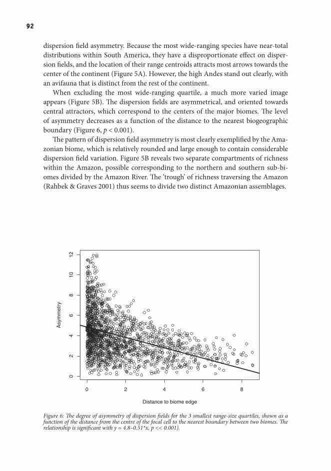
9292
dispersion field asymmetry. Because the most wide-ranging species have near-total distributions within South America, they have a disproportionate effect on disper-sion fields, and the location of their range centroids attracts most arrows towards the center of the continent (Figure 5A). However, the high Andes stand out clearly, with an avifauna that is distinct from the rest of the continent.
When excluding the most wide-ranging quartile, a much more varied image appears (Figure 5B). The dispersion fields are asymmetrical, and oriented towards central attractors, which correspond to the centers of the major biomes. The level of asymmetry decreases as a function of the distance to the nearest biogeographic boundary (Figure 6, p < 0.001).
The pattern of dispersion field asymmetry is most clearly exemplified by the Ama-zonian biome, which is relatively rounded and large enough to contain considerable dispersion field variation. Figure 5B reveals two separate compartments of richness within the Amazon, possible corresponding to the northern and southern sub-bi-omes divided by the Amazon River. The ‘trough’ of richness traversing the Amazon (Rahbek & Graves 2001) thus seems to divide two distinct Amazonian assemblages.
0 2 4 6 8
02
46
810
12
Distance to biome edge
Asy
mm
etry
Figure 6: The degree of asymmetry of dispersion fields for the 3 smallest range-size quartiles, shown as a function of the distance from the centre of the focal cell to the nearest boundary between two biomes. The relationship is significant with y = 4.8–0.51*x, p << 0.001).

93Species pools
DISCUSSION
We investigate the interaction between biome configuration and energy dynamics, taking a uniquely spatial approach to species turnover. This approach highlights how changes in species composition between communities are highly non-random in space, and offers a range of new possibilities. The method contrasts with previous studies that have focused on the mean turnover of a grid cell: A traditional approach has been to study mean values of assemblage similarity between a cell and its adja-cent cells (e.g. Gaston et al. 2007) or with all grid cells within a certain distance (e.g. Buckley & Jetz 2008). Alternatively, a method that focuses more on assemblage-wide patterns is to count the number of range boundaries that occur in a cell (McInnes et al. 2009). However, the limitation of such analyses is that they ignore the direction of turnover gradients. In allowing us to address such spatial relationships directly, dispersion field analysis is a powerful tool for identifying patterns in regional species assembly.
Applying dispersion field analysis to the avifauna of South America reveals a strong signal of biogeographic boundaries in the structure of species assemblages. Except for a small number of nearly cosmopolitan species, South American birds are structured into distinctive assemblages that mirror the spatial configuration of biomes. This creates characteristic patterns of species turnover, so areas close to the boundaries between biomes have much higher similarity with areas located nearer to the biome’s center. Such regionally distinct species assemblages are tangible expres-sion of species source pools, a concept which has otherwise been consistently difficult to pin down (Graves & Rahbek 2005).
The organization of the avifauna into distinct species pools explains why energy levels are not sufficient to explain the species richness of South America (Figure 3). Though there is a clear relationship between temperature and richness, highland forest biomes consistently have higher species numbers for the same temperature, whereas arid biomes have lower. This effect of regional species pools is not explicitly incorporated in metabolic theory, though Allen et al. (2002) pointed out that differ-ent regions may have different intercepts for the temperature-richness relationship. In fact, the importance of regional species pools for species-energy relationships was realized already by Wright (1983). He based his species-energy model on the equi-librium theory of island biogeography, which models species richness on islands as a joint function of area and isolation (MacArthur & Wilson 1967). Wright’s innovation was to substitute energy levels for area; energy would then interact with isolation to determine richness patterns. In this context, biogeographic barriers to species disper-sal could be interpreted as a continental parallel to island isolation.
The tenet of metabolic theory that energy levels correlate with richness because energy controls the rate of speciation implicitly assumes that speciation happens in situ. In South America, however, the highly clumped occurrence of small-ranged

9494
species points to a few areas such as the Northern Andes as cradles of speciation. The Andean region has a highly dynamic geological history, and have been shown in several studies to be hotspots of diversification for plants (Hughes & Eastwood 2006; Antonelli et al. 2009) and amphibians (Santos et al. 2009). The dynamic history and physical configuration of this region means that opportunities for vicariance and al-lopatric speciation are created often (Fjeldsa 1994)Graves 1985?. This pattern does not exclude a primary role for metabolic kinetics, as energetic control of metabolic processes may be instrumental in determining the rate with which such vicariance leads to actual speciation.
Certain caveats apply to this interpretation. First, the distribution of small-ranged species is not an unequivocal indicator of speciation rates (Jetz et al. 2004). Tropical mountains can either be ‘cradles’ (Stebbins 1974) where speciation rates are unusual-ly high; or they can be ‘museums’, where climatic stability allows relictual populations to persist after going extinct elsewhere (Fjeldsa 1994). Studies on the relative ages of montane taxa seem to indicate that mountains are both. Also, the relative absence of small-ranged species in the Amazon, where energy levels are among the highest in the world, does not mean that speciation does not occur there. Though there is very little data on the speed of post-speciation range expansion, marine studies indicate that they may be high (Liow & Stenseth 2007), so that newly evolved species in the Amazon, where dispersal barriers are few, could expand freely.
The implication of this is that metabolic theory could advance significantly by explicitly incorporating the scaling mechanics that link regional speciation processes to local energy dynamics. Regional differences in speciation rates interact with biome conservatism to create species pools. In local sites, communities with surplus energy are supplemented with the very widespread species, which are not constrained by the configuration of biomes. Such species may have evolved an ‘expansion’ phenotype (van Bocxlaer et al. 2010) that enables them to expand far outside their natal biome. Instead, widespread species have been shown to have high levels of cell-to-cell turn-over (Gaston et al. 2007), and to correlate highly with available energy (Jetz & Rahbek 2002; Evans et al. 2005). These species may depend on high energy levels to persist (Evans et al. 2005), as species with large ranges generally also have significantly more numerous local populations (Brown 1984; Borregaard & Rahbek 2010a). Thus, they may be responsible for the high predictive power of incoming energy on levels of spe-cies richness. Though relatively few, these very widespread species dominate species richness patterns in correlative analyses, as they contribute many more data points than other species (Jetz & Rahbek 2002).
95Species pools
METHODS
We used a data set describing the occupancy of all 2869 bird species breeding in South America in 1689 1° latitude-longitude grid cells, which has been the object of several previously published analyses (e.g. Graves & Rahbek 2005; Rahbek et al. 2007). The South American continent is ideal for continental studies of range patterns, as it is relatively well delimited, only adjoining the rest of the Americas along a narrow strip in the northwestern corner. For the minority of species (n = 643) that have ranges extending into Central and North America, we restricted our analyses to the range within South America. The resulting range sizes of South American birds vary by more than three orders of magnitude at the 1° scale used here. To investigate differ-ences between widespread and rare species, we divided all species into four quartiles based on their total range size, and performed separate analyses for each subset.
To compare the pattern of richness with that predicted by metabolic theory, we compared the species richness of birds to values of mean annual temperature. Tem-perature values were extracted from the mean monthly climatic database published by New et al. (1999), which was compiled globally at a 0.5° latitude-longitude resolu-tion for the period 1961-1990.
For each species, we calculated the range center, defined as the center of gravity of the distributional range. This was defined as:
where (xi, yi) are the coordinates of cells occupied by the species, and n is the number of occupied cells. Note that this definition means that the center of a range map may actually lie in an unoccupied cell. Though this is problematic if we wish to infer spa-tial processes around the range center for individual species, the measure is robust for use in mapping location of ranges to a geographical point for assemblage-wide analysis. We then generated dispersion fields for each grid cell, using the approach of Graves and Rahbek (2005). We calculated the center of gravity for each dispersion field, by taking the grand mean of the range center coordinates of all species occur-ring in the cell:
where N is the number of species occurring in the focal cell. We also calculated the mean range of each grid cell.
To describe the orientation of the dispersion field for a given grid cell, we calcu-lated the distance and angular direction from the focal cell to the center of the disper-sion field of that cell. We then used these data to express dispersion field assymetries on maps using ArcGIS. All calculations were done using custom-made software
, ,W SN
X
N
Yjj
N
jj
N
0 0=
= =^ eh o/ /
, ,X Yn
x
n
yii
ni
i
n
0 0= = =^ ch m/ /
9696
written in C++. The maps and figures were generated using R-2.10.1 (R 2009).
REFERENCES
Allen A.P., Brown J.H. & Gillooly J.F. (2002). Global Biodiversity, Biochemical Kinetics, and the Energetic-Equivalence Rule. Science, 297, 1545-1548.
Allen A.P., Gillooly J.F., Savage V.M. & Brown J.H. (2006). Kinetic effects of temperature on rates of genetic divergence and speciation. Proceedings of the National Academy of Sciences, 103, 9130-9135.
Antonelli A., Nylander J.A.A., Persson C. & Sanmartà n I. (2009). Tracing the impact of the Andean uplift on Neotropical plant evolution. Proceedings of the National Academy of Sci-ences, 106: 9749-9754.
Borregaard M.K. & Rahbek C. (2010a). Causality in the relationship between geographic distri-bution and species abundance. The Quarterly Review of Biology, 85, 3-25.
Borregaard M.K. & Rahbek C. (2010b). Dispersion fields, diversity fields and null models: unit-ing range sizes and species richness. Ecography, 9999.
Brown J.H. (1984). On the relationship between abundance and distribution of species. Ameri-can Naturalist, 124 255-279.
Brown J.H., Gillooly J.F., Allen A.P., Savage V.M. & West G.B. (2004). Toward a metabolic theory of ecology. Ecology, 85, 1771-1789.
Buckley L.B. & Jetz W. (2008). Linking global turnover of species and environments. Proceedings of the National Academy of Sciences, 105, 17836-17841.
Crisp M.D., Arroyo M.T.K., Cook L.G., Gandolfo M.A., Jordan G.J., McGlone M.S., Weston P.H., Westoby M., Wilf P. & Linder H.P. (2009). Phylogenetic biome conservatism on a global scale. Nature, 458, 754-756.
Evans K.L., Greenwood J.J.D. & Gaston K.J. (2005). Relative contribution of abundant and rare species to species-energy relationships. Biology Letters, 1, 87-90.
Fjeldsa J. (1994). Geographical patterns for relict and young species of birds in africa and south-america and implications for conservation priorities. Biodiversity and Conservation, 3, 207-226.
Gaston K.J., Davies R.G., Orme C.D.L., Olson V.A., Thomas G.H., Ding T.S., Rasmussen P.C., Lennon J.J., Bennett P.M., Owens I.P.F. & Blackburn T.M. (2007). Spatial turnover in the global avifauna. Proceedings of the Royal Society B-Biological Sciences, 274, 1567-1574.
Gillooly J.F. & Allen A.P. (2007). Linking global patterns in biodiversity to evolutionary dynam-ics using metabolic theory. Ecology, 88, 1890-1894.
Graves G.R. & Rahbek C. (2005). Source pool geometry and the assembly of continental avifau-nas. Proceedings of the National Academy of Sciences, 102, 7871-7876.
Hawkins B.A., Field R., Cornell H.V., Currie D.J., Guegan J.F., Kaufman D.M., Kerr J.T., Mit-

97Species pools
telbach G.G., Oberdorff T., O’Brien E.M., Porter E.E. & Turner J.R.G. (2003). Energy, water, and broad-scale geographic patterns of species richness. Ecology, 84, 3105-3117.
Hughes C. & Eastwood R. (2006). Island radiation on a continental scale: Exceptional rates of plant diversification after uplift of the Andes. Proceedings of the National Academy of Sci-ences, 103, 10334-10339.
Jetz W. & Rahbek C. (2002). Geographic range size and determinants of avian species richness. Science, 297, 1548-1551.
Jetz W., Rahbek C. & Colwell R.K. (2004). The coincidence of rarity and richness and the poten-tial signature of history in centres of endemism. Ecology Letters, 7, 1180-1191.
Liow L.H. & Stenseth N.C. (2007). The rise and fall of species: implications for macroevolution-ary and macroecological studies. Proceedings of the Royal Society B: Biological Sciences, 274, 2745-2752.
MacArthur R.H. & Wilson E.O. (1967). The theory of Island Biogeograph. Princeton University Press, Princeton.
McInnes L., Purvis A. & Orme C.D.L. (2009). Where do species’ geographic ranges stop and why? Landscape impermeability and the Afrotropical avifauna. Proceedings of the Royal Society B: Biological Sciences, -.
New M., Hulme M. & Jones P. (1999). Representing twentieth-century space-time climate vari-ability. Part I: Development of a 1961-90 mean monthly terrestrial climatology. Journal of Climate, 12, 829-856.
R D.C.T. (2009). R: A language and environment for statistical computing. In. R Foundation for Statistical Computing Vienna, Austria.
Rahbek C., Gotelli N.J., Colwell R.K., Entsminger G.L., Rangel T.F.L.V. & Graves G.R. (2007). Predicting continental-scale patterns of bird species richness with spatially explicit models. Proceedings of the Royal Society B-Biological Sciences, 274, 165-174.
Rahbek C. & Graves G.R. (2001). Multiscale assessment of patterns of avian species richness. Proceedings of the National Academy of Sciences, 98 4534-4539.
Ricklefs R.E. (2007). History and Diversity: Explorations at the Intersection of Ecology and Evolution. The American Naturalist, 170, S56-S70.
Ricklefs Robert E. (2008). Disintegration of the Ecological Community. The American Natural-ist, 172, 741-750.
Santos J.C., Coloma L.A., Summers K., Caldwell J.P., Ree R. & Cannatella D.C. (2009). Amazo-nian Amphibian Diversity Is Primarily Derived from Late Miocene Andean Lineages. PLoS Biol, 7, e1000056.
Stebbins G.L. (1974). Flowering plants: Evolution above the species level. Belknap Press of Har-vard University Press, Cambridge, MA.
Stegen J.C., Enquist B.J. & Ferriere R. (2009). Advancing the metabolic theory of biodiversity. Ecology Letters, 12, 1001-1015.
Stotz D.F., Fitzpatrick J.W., Parker T.A. & Moskovits D.K. (1996). Neotropical Birds. Ecology and conservation. University of Chicago Press, Chicago and London.

9898
van Bocxlaer I., Loader S.P., Roelants K., Biju S.D., Menegon M. & Bossuyt F. (2010). Gradual Adaptation Toward a Range-Expansion Phenotype Initiated the Global Radiation of Toads. Science, 327, 679-682.
Wiens J.J. & Donoghue M.J. (2004). Historical biogeography, ecology and species richness. Trends in Ecology & Evolution, 19, 639-644.
Wiens J.J. & Graham C.H. (2005). Niche conservatism: Integrating evolution, ecology, and con-servation biology. Annual Review of Ecology, Evolution, and Systematics, 36, 519-539.
Wright D.H. (1983). Species-energy theory - an extension of species-area theory. Oikos, 41, 496-506.

Published as a book chapter:Borregaaard, M. K., Hendrichsen, D. K. and Nachman, G. N. 2009.
Spatial distribution. In: Encyclopedia of Ecology, edited by S.-E. Jørgense. Elsevier.
Chapter 5:Spatial distribution

100

101Author's personal copy
Spatial DistributionM K Borregaard, D K Hendrichsen, and G Nachman, University of Copenhagen, Copenhagen, Denmark
ª 2008 Elsevier B.V. All rights reserved.
The Distribution of Organisms Over Landscapes
Dispersion of Individuals
Biological Impacts on Spatial Patterns
Processes Mediated by Spatial Structuring of
Populations
Large-Scale Distribution Patterns
Summary
Further Reading
Organisms do not occur randomly in space. Any species ofplant or animal may be found in some areas, while theyare completely absent from others. Likewise, the indivi-duals of any one species are distributed in relation to eachother in distinct patterns. The reasons for the readilyapparent nonrandomness of the spatial distribution pat-terns of organisms are numerous, and the patterns resultfrom processes acting throughout the whole life cycle ofthe organism, and on various spatial scales. Although thisspatial structuring of populations is often ignored in eco-logical theory, it has profound implications for themediation of biological processes: interactions betweenindividuals and across species all take place in space aswell as in time, and an understanding of spatial patterns isbasic to understanding real-life ecological processes.Indeed, patterns of spatial distribution play an importantrole in shaping a wide range of ecological dynamics, suchas intra- and interspecific competition, mating systems,predation, population genetics, and the spread of conta-gious diseases.
This article presents an overview of how spatial pat-terns in the distribution of organisms are created, andhow they influence the way ecological processes runtheir course in ecological communities, exemplified bypredator–prey dynamics. These patterns are scale depen-dent: organisms which are distributed in one way whenobserved at a large spatial scale may be distributed verydifferently at closer scales. To accommodate this, thepresentation is structured according to the main spatialscale of the patterns under discussion. The initial focuslies on the way organisms are distributed at a landscapelevel, at which spatial distribution is mainly influenced bytopographical features and variation in habitat availabil-ity. The subsequent discussion moves the scale to patternsin the dispersion of individuals, which can be seen pri-marily as an effect of behavioral interactions withconspecifics and with those of predator and prey species.To conclude, large-scale regional distribution patternsare briefly discussed, in relation to how they may con-tribute to the observed spatial distribution patterns atsmaller scales.
The Distribution of Organisms OverLandscapes
An organism may only persist where the physical condi-tions (temperature, humidity, etc.) are tolerable and thefood resources are adequate. In other words, the environ-ment should match the niche space of the species (seeEcological Niche). Consequently, all organisms are asso-ciated with a specific type of habitat, and hence view thearea around them in widely different manners. In thiscontext, it is useful to think of the landscape as a mosaic,consisting of patches of favorable habitat surrounded byuninhabitable areas. Within such patches the species mayform more or less permanent local populations (alsocalled subpopulations), while the species is only rarelyfound in the intervening areas.
The dynamics of a subpopulation are driven by severalprocesses, as shown in Figure 1. Individuals enter thepopulation through birth and immigration, and leave itas a result of death and emigration. Of these processes,birth and death rates may be controlled by the number ofindividuals already present, their density, and theresource availability. Immigration and emigration mayalso be affected by these factors, as well as by the favor-ability of the surrounding landscape and the size of theadjacent subpopulations.
If we increase our vantage point to include severalsuch subpopulations located over the landscape, whichare separated by uninhabitable areas but with migrationoccurring between them, then a very complex pictureappears (Figure 2). All these interacting subpopulationscan be viewed as one large spatially structured popula-tion, known as a metapopulation (see MetapopulationModels). The complex spatial dynamics of the metapo-pulation result from the patterns of between-patchmovement and local birth and death rates, as well aslocal extinction and colonization of subpopulationswhich occur over larger timescales. These processescan be modeled by a set of connected differential equa-tions, which allows quantitative predictions to be madeabout the dynamics of the metapopulation.
3304 Population Dynamics | Spatial Distribution

102Author's personal copy
Other factors, which are not accounted for by the basicmodel described above, may be included in more sophisti-
cated representations. These factors include the size andfavorability of patches, their relative isolation, and the
nature of the intervening habitat relative to the dispersalability of the organism. There are also dynamic processesaffecting the occupancy of each patch over time. These
processes rely on the observation that over time, the sub-population in many cases causes a reduction in the quality
of the patch which it inhabits (e.g., reduces the amount ofresources and/or attracts predators, parasites, and patho-gens). As the environment deteriorates, mortality and
emigration is likely to increase while the rate of reproduc-tion correspondingly decreases. In addition, Allee effects(see later) can hasten the demise of the subpopulation.
A further complication to this pattern is that these effectsare not restricted to the species in question, but are equally
likely to affect its predators and the vital bioresources, suchas food resources on which it depends.
An interesting consequence of the spatial movement ofindividuals between subpopulations is that some patchesmay be occupied, even though they cannot in themselvessustain viable populations of the species. The subpopula-tion of such a patch is actually kept alive by theimmigration of individuals from more productive patchesin the vicinity. The movement of individuals resembleswater flowing from its source to a sink, and correspond-ingly this type of system is usually termed source–sinkdynamics (see Dispersal–Migration). In some areas, espe-cially in transition zones between habitats or biomes andin areas severely affected by human disturbance, suchsource–sink dynamics may play a key role in structuringthe occurrence and distribution of individuals.
Dispersion of Individuals
An alternative way of describing spatial distributions is tomove the focus to the position of separate individuals inspace. When viewed from above, the distribution of indi-viduals over the landscape can be visualized as a patternof tiny dots dispersed over a blank area. This pattern mayin theory be completely random, but usually individualsare either clumped together, or at the opposite, spread outin a regular fashion (see Figure 3).
Empirically, dispersion patterns can be characterized bythe average number of individuals in randomly sampledunits of area within the landscape �xð Þ and the variancebetween number of individuals occurring per samplingunit (s2). The ratio s2=�x is commonly known as the indexof dispersion. In randomly distributed populations, theindex of dispersion is approximately equal to 1 (see Box 1).
Clearly, dispersion patterns are strongly dependentupon the scale at which they are perceived – for instance,the distribution of an insect species living on leaves oftrees can be studied on many different spatial scales, suchas the distribution on each leaf, among leaves within abranch, among branches within a tree, and between treeswithin a forest.
From the beginning, it seems obvious that there shouldbe some clumping of individuals – organisms do notappear out of the thin air. Each individual originatesfrom a parent, and as such appears in close vicinity toother individuals, which in most cases are relatives. Afterbirth, or at a later stage in the life cycle, they undergosome juvenile dispersal (see Dispersal–Migration) beforesettling down in a favorable location, but some degree ofaggregation is still retained. Another factor which predis-poses for aggregation is that individuals of the samespecies are attracted to a set of conditions and resources,which are themselves patchily distributed.
Aggregated dispersion patterns are very common innature. An example of an extremely aggregated species is
Births
Deaths
Emigration
Immigration
Figure 1 The abundance of a subpopulation within a patch ofsuitable habitat is affected by the processes of birth, death,
immigration, and emigration.
Figure 2 In a landscape consisting of several suitable habitatpatches, the population dynamics become dependent on dispersal
and colonization between interconnected subpopulations. Such a
system is described by metapopulation dynamics.
Population Dynamics | Spatial Distribution 3305

103Author's personal copy
the Kashmir cave bat (Myotis longipes), which is onlyknown from nine localities in the Himalaya region, eachhome to populations of a thousand individuals or more.
A regular or even distribution, on the other hand, is theresult when individuals compete for limited resources.
This type of pattern is commonly exhibited by manysessile organisms such as trees, which space themselvesevenly as a result of competition for water or sunlight.Also many animals have approximately regular distribu-tions – a familiar example is the territories of songbirds.
Figure 3 A schematic representation of the dispersion of individuals in a subpopulation with (from left to right) either a regular
s2 < �x� �
, a random s2 � �x� �
, or a clumped s2 > �x� �
distribution.
Box 1 Analysis of spatial data
As the null hypothesis, it is assumed that individuals in a population are randomly distributed among the n sampling units of a sample. Ifthis is the case, it is expected that the variance should equal the average so that the ‘index of dispersion’, s2/x, is approximately equal to 1.If the ratio exceeds 1, it indicates that the population has a patchy (or clumped) distribution whereas a value less than unity indicates aneven (or regular) distribution. However, since data originate from sampling, they will always be associated with some variation, so it islikely that some deviation in s2/x from unity will occur even if the underlying distribution is random. Especially if the sample size n issmall, s2/x will exhibit large variation due to sampling noise. A �2-test can be used for testing whether s2/x deviates significantly from 1since �2¼ (n�1)s2/x with n�1 degrees of freedom. It should be noted that the test is two-tailed (in contrast to the majority of cases where�2-tests are used) since values significantly smaller or larger than n�1 can lead to rejection of the null hypothesis.
Though the index of dispersion indicates whether a population is evenly, randomly, or patchily distributed in space, it does notexplicitly reveal information about the underlying spatial distribution. This requires that the empirical distribution of sampling units with x
individuals can be fitted by a theoretical ‘probability function’ called P(x), which denotes the probability that a randomly selected spatialunit contains exactly x individuals. As all probability functions, P(x) for all possible integer values of x equal to or larger than 0 should sum tounity.
The Poisson distribution is used to describe the underlying distribution when it is random, the positive binomial distribution when it iseven and the negative binomial distribution when it is clumped. However, other less frequently used distributions are also available tomodel clumped populations, for example, the Thomas distribution, the logarithmic series distribution, the Polya–Aeppli distribution, andNeyman’s type A, B, and C distributions. Once an adequate probability function has been identified and fitted to data, the quality of the fitcan be assessed by means of a goodness-of-fit test, usually a �2 one-sample test or a Kolmogorov–Smirnov one-sample test.
A problem often encountered in analyzing spatial data statistically is the fact that they do not represent independent observations.Thus, if sampling unit i is separated from sampling unit j by a distance dij, it seems likely that xiwill be more similar to xj, the smaller the dij is.This phenomenon is known as ‘spatial autocovariation’. Spatial autocovariance is often depicted as a so-called ‘semivariogram’ wherethe ‘semivariance’ (�d) is plotted against d. The semivariance at distance d is calculated as �d¼
Pi¼1nd (xi+d� xi)
2/2nd,where xiþd is the valueof x measured at distance d from another measurement xi and nd is the number of measurements separated by distance d.
Spatial patterns can be depicted graphically by means of a technique known as ‘kriging’. The principle is to place a large number ofpoints spaced out over the entire area under study. Each point is characterized by its coordinates in the two-dimensional x–y space, andby the value of a given attribute (for instance the population density in the area around the point). The value of the attribute is denoted the zcoordinate, which represents a height above the x–y plane. Hence, small and large values of zwill appear as troughs and peaks in a three-dimensional (3-D) landscape. 3-D landscapes can be projected into two-dimensional (2-D) landscapes by means of contour plots wherepoints with identical z-values are connected with lines (isoclines), similar to how temperature and atmospheric pressure are depicted inmeteorological maps. The more fine-grained the information is, the more precise the map will be. Various algorithms have beendeveloped to interpolate values between neighboring points so as to estimate z in points that have not been sampled, and to smoothout the landscape by removing local peaks and troughs caused by sampling noise.
Since kriging is computationally demanding, various specialized software products exist to perform it, for example, easy_krig, DACE,GSþ. In addition, kriging can be handled by some statistical packages, such as R.
3306 Population Dynamics | Spatial Distribution

104Author's personal copy
Biological Impacts on Spatial Patterns
As mentioned above, the dispersion pattern of indivi-duals is affected by the structure of the landscape andthe resource demands of the organism. Theoretically, ifindividuals were similar and completely free to move,they would be dispersed over the landscape so that eachindividual had the same access to the resource. Thispattern is known as the ideal free distribution, and willsimply reflect the instantaneous distribution of resources.However, differences between the competitive abilitiesof individuals, habitat barriers hindering free movement,and the individuals’ lack of perfect knowledge about thedistribution of resources all contribute to making exam-ples of populations following the ideal free distributionrare in nature.
The behavior and life styles of organisms are extre-mely varied, and patterns of spatial distribution exhibit agreat deal of variation. Mobile organisms move around inorder to acquire resources and may also engage in socialinteractions with conspecifics. This means that behavioralchoices play a profound role in shaping occurrence pat-terns. One of the most obvious cases of this effect is thecongregation into cooperative flocks seen in many animalspecies. The exact nature of these flocks differs widelyamong organisms – from the loose aggregations of restingbrent geese (Branta bernicla), via the socially complexcooperative units of wolf (Canis lupus) packs to thesuper-individual hive structure of eusocial insects.
Optimal Group Size
Despite the great variation in types of animal groups, thebiology of flock behavior has important commonalitiesacross all species. An example is the determinants ofgroup size, which can be seen as a function of the costsand benefits of being part of a group.
A group consisting of N individuals can increase itssize without recruitment of individuals from outside aslong as the group’s per capita growth rate r in eqn [1] ispositive:
dN
dt¼ rN ½1�
r is likely to be a function of group size, reflecting thedifference between benefits and costs of adding furtherindividuals to the group. Hence, r may be modeled as adifference between two functions:
r Nð Þ ¼ benefits – costs ¼ f Nð Þ – g Nð Þ N � 1ð Þ ½2�
where f (N) denotes the benefit function and g(N) the costfunction. Both functions can either be independent ofN orincrease with N. Since groups cannot be infinitely large,there will exist a value for N satisfying the condition that
r(N)¼ 0 for N¼Nmax and r(N) < 0 for N>Nmax. Benefitsof increasing group size are likely to level off with N,while costs are likely to accelerate as N becomes large asindicated in Figure 4a. Nmax corresponds to the value ofN when costs and benefits balance.
When group size reaches its maximum size, r will be 0,indicating that the fitness of group members is low. By
reducing group size from this point, the fitness of each
–1
0
1
2
3
4
5
Rat
es
B C
r
Nmax
(a)
–0.4
–0.2
0
0.2
0.4
0.6
0.8
1
1.2
1.4
Rat
es
BC
r
(b)
10 20 30 40 50 60Group size (N )–0.5
0
0.5
1
1.5
2
Rat
es
B C
rNopt
Nmax
(c)
10 20 30 40
Group size (N )
10 20 30 40 50 60Group size (N )
Nopt
Nopt
Nmax
Nmin
50 60
Figure 4 Group formation is predicted to occur when therelative growth rate (r) increases with group size. Depending on
how the benefits (B) and costs (C) of group behavior change with
group size (N), three different cases can be identified: (a) Benefits
increase more steeply than costs when group size is small, andvice versa when group size is large, leading to an optimal group
size (Nopt) toward which the group is predicted to converge. If a
group does not split up whenN>Nopt, it will continue to grow until
N¼Nmax. (b) Solitary behavior (i.e., N¼1) is predicted if costsincrease more than benefits as group size increases. (c) A group
must be larger thanNmin in order to persist and grow, whereas it is
goes toward to extinction ifN falls belowNmin because the relativegrowth rate is negative (the so-called Allee effect).
Population Dynamics | Spatial Distribution 3307

105Author's personal copy
individual will increase. The optimal group size (denotedNopt) is reached when r is at maximum (Figure 4b). If Nopt
is close to 1, individuals will gain by living alone, forinstance, in territories, and their spatial distribution willtend to be regular or random. In contrast, species withhigh values of Nopt will be patchily distributed. This willapply to species that can adjust their group size in accor-dance to net benefits, for instance, in animals whereindividuals can join (if N<Nopt) or leave groups (ifN>Nopt). If groups are not formed by such behavioralmechanisms, as with plants, group size will continue togrow until N¼Nmax. A special case of eqn [2] is whenbenefits and costs balance at two different group sizes, asshown in Figure 4c. When N is below Nmin, the group willgo extinct because the smaller the group the more nega-tive r becomes (the so-called Allee effect) (see AlleeEffects). The only way the extinction of such a groupcan be avoided is by recruiting individuals from outside.
Population-Level Variation in DispersionPatterns
As noted above, the behavioral life styles of animalsdetermine their distribution. While some animals, suchas the wildebeest (Connochaetes taurinus), live in groupsthat migrate over large areas or restrict their dispersal toextended home ranges, many others are territorial, divid-ing the available habitat into separate areas which aredefended against the intrusion of conspecifics.
In addition, different members of a population mayexhibit widely different patterns of dispersion, resultingin highly complex overall spatial patterns. Territoriality,for instance, causes all reproducing individuals to adhereto a regular dispersion pattern – but for nonreproducingindividuals the situation may be very different.
An example is provided by the tawny owl (Strix aluco)which is a long-lived, monogamous, territorial bird(Figure 5). Juveniles only get access to optimal resourceswhen adults die and thereby leave vacant territories.Adults defend their territories fiercely against intruders,though they are more willing to accept juveniles withinthe territory boundaries during July and August, when thejuveniles disperse from their natal territories.
This difference between the lifestyles of adults andjuveniles means that only few individuals survive toreach adulthood. Adult birds within their territorieshave a relatively high survival; telemetry studies showthat a main cause of death within the fragmented land-scapes of Western Europe is traffic. The juveniles, on theother hand, are vulnerable to a range of factors. Since theyhave no territory, they are forced to move around andhunt in unknown areas and marginal habitats where sur-vival chances are poorer (Figure 6). They are also morevulnerable to predators. Because only individuals posses-sing a territory can breed, the density of breeding animals
500 m
Owl 91
Night locationsDay locationsDeciduous forestConiferous forestBuild-up areasOpen land95% Minimum convex polygon95% Kernel
Figure 5 Habitat map showing observations of juvenileindividuals of tawny owl (Strix aluco) in a mosiac landscape of
agricultural land, forest, and urban areas. The minimum convex
polygon and the Kernel denote different methods of establishing
the core area used by an individual or a group of individuals, andprovide information on the habitat preferences, home range, and
territory boundaries. Copyright: Peter Christiansen and Peter
Sunde, unpublished data.
Figure 6 Juvenile tawny owls (Strix aluco) live a precarious life
as vagrants while they are waiting to take over a vacant territorywhen an adult individual dies. Copyright: Peter Christiansen.
3308 Population Dynamics | Spatial Distribution
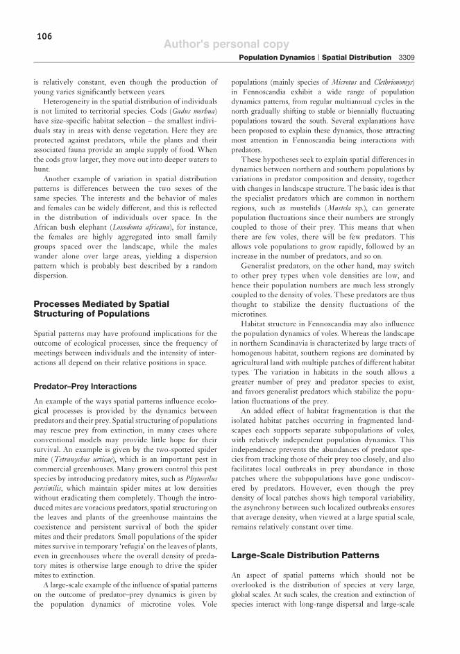
106Author's personal copy
is relatively constant, even though the production ofyoung varies significantly between years.
Heterogeneity in the spatial distribution of individualsis not limited to territorial species. Cods (Gadus morhua)have size-specific habitat selection – the smallest indivi-duals stay in areas with dense vegetation. Here they areprotected against predators, while the plants and theirassociated fauna provide an ample supply of food. Whenthe cods grow larger, they move out into deeper waters tohunt.
Another example of variation in spatial distributionpatterns is differences between the two sexes of thesame species. The interests and the behavior of malesand females can be widely different, and this is reflectedin the distribution of individuals over space. In theAfrican bush elephant (Loxodonta africana), for instance,the females are highly aggregated into small familygroups spaced over the landscape, while the maleswander alone over large areas, yielding a dispersionpattern which is probably best described by a randomdispersion.
Processes Mediated by SpatialStructuring of Populations
Spatial patterns may have profound implications for theoutcome of ecological processes, since the frequency ofmeetings between individuals and the intensity of inter-actions all depend on their relative positions in space.
Predator–Prey Interactions
An example of the ways spatial patterns influence ecolo-gical processes is provided by the dynamics betweenpredators and their prey. Spatial structuring of populationsmay rescue prey from extinction, in many cases whereconventional models may provide little hope for theirsurvival. An example is given by the two-spotted spidermite (Tetranychus urticae), which is an important pest incommercial greenhouses. Many growers control this pestspecies by introducing predatory mites, such as Phytoseiluspersimilis, which maintain spider mites at low densitieswithout eradicating them completely. Though the intro-ducedmites are voracious predators, spatial structuring onthe leaves and plants of the greenhouse maintains thecoexistence and persistent survival of both the spidermites and their predators. Small populations of the spidermites survive in temporary ‘refugia’ on the leaves of plants,even in greenhouses where the overall density of preda-tory mites is otherwise large enough to drive the spidermites to extinction.
A large-scale example of the influence of spatial patternson the outcome of predator–prey dynamics is given bythe population dynamics of microtine voles. Vole
populations (mainly species of Microtus and Clethrionomys)in Fennoscandia exhibit a wide range of populationdynamics patterns, from regular multiannual cycles in thenorth gradually shifting to stable or biennially fluctuatingpopulations toward the south. Several explanations havebeen proposed to explain these dynamics, those attractingmost attention in Fennoscandia being interactions withpredators.
These hypotheses seek to explain spatial differences indynamics between northern and southern populations byvariations in predator composition and density, togetherwith changes in landscape structure. The basic idea is thatthe specialist predators which are common in northernregions, such as mustelids (Mustela sp.), can generatepopulation fluctuations since their numbers are stronglycoupled to those of their prey. This means that whenthere are few voles, there will be few predators. Thisallows vole populations to grow rapidly, followed by anincrease in the number of predators, and so on.
Generalist predators, on the other hand, may switchto other prey types when vole densities are low, andhence their population numbers are much less stronglycoupled to the density of voles. These predators are thusthought to stabilize the density fluctuations of themicrotines.
Habitat structure in Fennoscandia may also influencethe population dynamics of voles. Whereas the landscapein northern Scandinavia is characterized by large tracts ofhomogenous habitat, southern regions are dominated byagricultural land with multiple patches of different habitattypes. The variation in habitats in the south allows agreater number of prey and predator species to exist,and favors generalist predators which stabilize the popu-lation fluctuations of the prey.
An added effect of habitat fragmentation is that theisolated habitat patches occurring in fragmented land-scapes each supports separate subpopulations of voles,with relatively independent population dynamics. Thisindependence prevents the abundances of predator spe-cies from tracking those of their prey too closely, and alsofacilitates local outbreaks in prey abundance in thosepatches where the subpopulations have gone undiscov-ered by predators. However, even though the preydensity of local patches shows high temporal variability,the asynchrony between such localized outbreaks ensuresthat average density, when viewed at a large spatial scale,remains relatively constant over time.
Large-Scale Distribution Patterns
An aspect of spatial patterns which should not beoverlooked is the distribution of species at very large,global scales. At such scales, the creation and extinction ofspecies interact with long-range dispersal and large-scale
Population Dynamics | Spatial Distribution 3309

107Author's personal copy
differences in climate to generate patterns of speciesrichness and control the composition of regional speciespools. Over time, new patterns are created as speciesexpand into new areas while going extinct in others, andas isolated subpopulations give rise to new species due toevolution.
The basic unit of large-scale ecology is the geographicdistribution range. Ranges can be represented in manyways, from the colored blotches known from popular fieldguides to exact mapping of territories and point counts ofindividual locations, and the definition of ranges is, likemost spatial patterns, strongly scale dependent.
The concept of ranges and their distribution hasattracted considerable attention in recent years, becauseof their profound importance for biodiversity. Identifyingand describing patterns of overall species richness and thelocation of areas with large numbers of endemics (i.e.,species with small range sizes) play a key role in theconservation and management of nature, since they areinstrumental in directing conservation efforts to the mostoptimal areas. In addition, an understanding of thesepatterns is at the center of attempts to predict the resultof the recent changes in diversity following human habitatdestruction and global warming (see Climate ChangeModels). These patterns all result from the location ofspecies ranges and the manner in which they overlap.
What determines large-scale distribution patternsremains the subject of debate: a long-standing controversyin ecology regards whether the size and location of spe-cies’ ranges are primarily decided by contemporaryecological (mainly climatic) factors, or by the interactionof dispersal and competition with other species present inthe area.
The shape and location of the range at large scales arealso mirrored by the distribution of individuals at smallerscales. Toward the edges of a range, populations of thespecies tend to become more patchily distributed, withmore widely separated individual subpopulations.Additionally, peripheral populations are smaller and sup-port fewer individuals, so that the abundance andoccupancy of the species co-vary across the range. Whatcreates this pattern is not completely known, but it seemslikely that it reflects that the density of habitats withoptimal conditions for the organism is higher in the corearea than in the periphery.
In this way, large-scale patterns interact with localprocesses, behavior, and biotic interactions to producethe distributions of plants and animals in nature. Thecomplexity of these distributions underline the increasingrealization that a consideration of spatial patterns is a vitalpart of any comprehensive framework for biology.
Summary
Patterns in the spatial distribution of organisms are extre-mely varied, and are affected by numerous factors in theecology and behavior of species. Distribution patterns notonly differ between species as a result of differences introphic level and relative commonness, but may also varywith the age, sex, and social status of individual organisms.Nonetheless, the overall patterns can be described usingrelatively simple models, providing a key factor for theunderstanding of ecological processes such as the rela-tionships between predator and prey populations.
See also: Allee Effects; Biodiversity; Climate Change
Models; Dispersal–Migration; Habitat Selection and
Habitat Suitability Preferences; Individual-Based Models;
Landscape Modeling; Mating Systems; Metapopulation
Models; Prey–Predator Models; Social Behavior.
Further Reading
Andreawartha HG and Birch LC (1954) The Distribution and Abundanceof Organisms. Chicago: University of Chicago Press.
Hanski I and Henttonen H (2002) Population cycles of small rodents inFennoscandia. In: Berryman A (ed.) Population Cycles. The Casefor Trophic Interactions, pp. 44–68. Oxford: Oxford UniversityPress.
Jongman RHG, Ter Braak CJF, and van Tongeren OFR (eds.) (1995)Data Analysis in Community and Landscape Ecology. Cambridge:Cambridge University Press.
Ranta E, Lundberg P, and Kaitala V (2006) Ecology of Populations.Cambridge: Cambridge University Press.
Rhodes OE, Chesser RK, and Smith MH (eds.) (1996) PopulationDynamics in Ecological Space and Time. Chicago: University ofChicago Press.
Rosenzweig ML (1995) Species Diversity in Space and Time.Cambridge: Cambridge University Press.
Stenseth NC and Lidicker WZ (eds.) (1992) Animal Dispersal – SmallMammals as a Model. New York: Chapman and Hall.
Tilman D and Kareiva P (eds.) (1997) Monographs in Population Biology30: Spatial Ecology. Princeton, NJ: Princeton University Press.
3310 Population Dynamics | Spatial Distribution

108

Manuscript, currently in revision with Ecography
Appendix I:Range size patterns in European
freshwater trematodes

110

111
Range size patterns in European freshwater trematodes
david W. thieltgesDepartment of Zoology, University of Otago
christiaN hofCenter for Macroecology, Evolution & Climate, University of Copenhagen
Michael K. Borregaard, Center for Macroecology, Evolution & Climate, University of Copenhagen
d. Matthias dehliNg Department of Ecology, Philipps-Universität Marburg, Germany
MartiN BräNdle Department of Ecology, Philipps-Universität Marburg, Germany
rolaNd BraNdl Department of Ecology, Philipps-Universität Marburg, Germany
roBert PouliNDepartment of Zoology, University of Otago
ABSTRACT
While patterns in geographic range sizes in free-living species have received much attention, little is known on the corresponding patterns in parasites. For the first time, we report on patterns in geographic range sizes and dimensions of endoparasites, using published species lists of freshwater trematodes in 25 bio-geographic regions of Europe. In general, the range sizes of trematodes showed a typical hollow curve frequency distribution, with most species having small ranges. Contrary to expectations, there were no differences in range sizes among trematodes using hosts with high (birds) and limited (e.g. fish) dispersal capac-ity. This suggests that the well known importance of host dispersal capacity for parasite dispersal at small local spatial scales is overridden by other factors on larger continental scales. Regression analyses and Rohde plots showed that the relationship between the latitudinal centre and range size was hump-shaped in

112112
all host groups except for reptiles, for which it was linear. Most of the variation fell within the expectations given by null models, suggesting that the patterns mainly result from the geographic properties of the European continent and the biogeographic regions. Finally, trematode ranges tended to stretch more in east-west than in north-south directions, indicating dispersal barrier effects for para-site faunas, probably due to the orientation of major geographical features such as the Alps.
INTRODUCTION
There is substantial variation in the size of the geographic ranges of species, span-ning up to 12 orders of magnitude (Brown et al. 1996). Species with very limited distributions, e.g. confined to oceanic islands, lie at one end of the spectrum. At the other end are cosmopolitan species with extremely large range sizes, spreading over much of the globe. This includes many marine animals like algae, jellyfish, fish, sea-birds and cetaceans have wide distributions throughout the marine realm (Gaston 2003). Within any taxonomic group, this variation in the size of geographic ranges can be visualised with a frequency distribution of the species-specific range sizes. Most groups of plants and animals show a unimodal distribution of range sizes with a strong right skew, sometimes called the “hollow curve” (Willis 1922, MacDonald 2003). This means that the majority of species within a taxon have small to medium geographic range sizes and only a few species have very large ranges.
While the hollow curve distribution of species’ geographic range sizes is a univer-sal pattern, the mean size of geographic ranges differs among major phylogenetic lin-eages. Within the vertebrates, freshwater fish have the smallest range sizes, followed by, in increasing order, amphibians, reptiles, mammals and birds (Anderson 1977, 1984a,b, Anderson and Marcus 1992, Brooks et al. 2001). There are also patterns in range size variation within taxonomic groups. For example, the range sizes of species tend to decrease from high to low latitudes, a phenomenon known as Rapoport’s rule (Stevens 1989). Geographic ranges may not only vary in extent but also in shape, i.e. ranges do not necessarily have the same extent in all dimensions. For example, Major biogeographic barriers or large-scale climatic zones can restrict the contours of spe-cies’ ranges (Brown and Maurer 1989). However, geographic patterns in species rich-ness may also simply result from the geometric properties of the study area, resulting in the so-called mid-domain effect, which can be tested using null models (Colwell and Hurtt 1994, Colwell and Lees 2000, Colwell et al. 2004).
Whereas patterns in geographic range sizes of free-living species have received much interest, little is known about the geographic range sizes of parasites. Some studies have found a positive correlation between the range sizes of hosts and the
113Range sizes in trematodes
numbers of parasite species infecting these hosts (Dritschilo et al. 1979, Gregory 1990, Brändle and Brandl 2001, Krasnov et al. 2004). However, to our knowledge only two related studies to date have investigated patterns in geographic range sizes of parasites themselves. The geographic ranges of ectoparasitic fleas (Siphonaptera) from small mammals show the same hollow curve distribution as seen in free-living species (Krasnov et al. 2005, 2008). The geographic range size of flea species was negatively correlated with their degree of host specificity, i.e. highly host specific flea species had smaller ranges than generalists that infect a wide range of host species (Krasnov et al. 2005). However, host specificity is not the only determinant of the size of geographic ranges of parasites. As parasites, depend on their hosts for dispersal, the dispersal capacity of the hosts should be strong determinants of the size of geo-graphic ranges of parasites. In parasites with complex life cycles, like digenean trema-todes, definitive hosts should be most relevant in this respect, as adult worms inside definitive hosts are the main dispersal stage of the parasites. The first intermediate hosts of trematodes are molluscs, which have a very limited dispersal capacity (plank-tonic larval stages are not infected). The second intermediate hosts are invertebrates, amphibians or fish, all of which again have limited dispersal capacity. Definitive hosts of trematodes are always vertebrates, which carry the adult parasites and disperse the parasites via their eggs shed with faeces. In general, the dispersal capacity of parasites in bird definitive hosts is considered to be higher than that of parasites utilising fish and other less vagile definitive hosts (Esch et al. 1988), an assumption supported by data on population genetics (Criscione and Blouin 2004). Hence, we expect parasites using freshwater fish as definitive hosts to have, on average, the smallest range sizes, and parasites utilising birds to have the largest range sizes within a regional assem-blage of trematodes.
In this study, we investigate patterns in range sizes and dimensions in European freshwater trematodes. Besides determining the frequency distributions of trema-tode range sizes, we investigate whether the range sizes of trematode species are de-termined by the dispersal capacity of their definitive hosts. To the best of our knowl-edge, both have not been investigated in endoparasites. Also, other patterns in range sizes of parasites like Rapoport’s rule or the dimensional shapes of parasites’ ranges have, as far as we know (other than the flea study mentioned above), not been studied to date. Based on the published distributions of trematodes over 25 biogeographical regions in Europe, we ask the following questions: 1) Do the range sizes of trema-todes exhibit the typical hollow curve distribution known from free-living species?, 2) Do the mean range sizes of trematodes differ depending on the type of definitive host they use?, 3) Are the range sizes of trematodes larger at higher latitudes (Ra-poport’s rule)? and 4) Do the shapes of the ranges of trematodes in Europe follow major topographic features like the Alps?

114114
MATERIALS.AND.METHODS
The data set used for the analyses was extracted from the Limnofauna Europaea (Il-lies 1978), using the data on presence/absence of digenean trematodes in each of 25 bioregions. All trematode species included in these tables spend at least the first part of their life cycle in freshwater habitats, i.e. the first intermediate host is always a freshwater mollusc. For each trematode species, we extracted information on the type of definitive hosts used from the original tables in the book: 1) fish, 2) amphib-ians, 3) reptiles, 4) mammals, 5) birds and mammals (in the case of trematode species that can use either), and 6) birds. Species with unknown type of definitive host were excluded from the analyses. In addition to information on the parasites we acquired geographic data on the 25 biogeographic regions. For each biogeographic region, as defined in the book, we determined the northern and southern as well as the eastern and western boundaries using http://earth.google.com/ and calculated the latitudinal and longitudinal ranges of each region from these data (Table 1; see Hof et al. 2008 for a map). In addition, using GIS, we calculated the area of each bioregion (Table 1).
Based on these data, we calculated various geographic range measures for each trematode species: 1) number of biogeographic regions in which each species was recorded; 2) total area occupied by each trematode species; 3) latitudinal and longi-tudinal range (degrees), using the boundaries of the northern-, southern-, western- and eastern-most regions in which each species occurred; and 4) dimensional shapes of each range (maximum north-south and east-west extent in km), using great circle calculations. Since the distance between longitudinal bands depends on latitude, we identified the eastern and western longitudinal extremes of the range and calculated the distance between them at the mean latitude of the species’ range.
To visualise the geographic ranges of the European freshwater trematode species, we plotted the frequency distribution of range sizes, separately for each major host group, using the total number of regions occupied by each species as this measure is least vulnerable to area overestimation (see discussion). We tested for differences in the mean range of trematode species utilising different definitive host groups with one-way ANOVAs (type 3 SS), using log-transformed data of 1) number of regions occupied by each species, 2) total area occupied, 3) latitudinal range and 4) longi-tudinal range. Post-hoc comparisons were conducted with Tukey’s HSD tests (for unequal n).
To investigate the relationships between the latitudinal centres of each species’ range and the total area occupied by the species (log-transformed), we used regres-sion analyses and Rohde plots (named after Rohde 1993, although this type of plot was originally introduced by Graves 1985). For the regression analyses, we includ-ed simple and squared latitudinal centre as independent variables, since plots of log(area) vs. latitudinal centre suggested a hump-shaped relationship. For the Rohde plots, we divided the geographic domain into latitudinal bands of 3° width. Within

115Range sizes in trematodes
each of these bands, we calculated the mean log(area) of all species whose latitudinal centre falls within this band (for details, see Rohde et al. 1993).
Because the shape of Europe constrains the possible locations and shapes of geographic ranges, a hump-shaped relationship between latitude and range size is expected even in the absence of ecological processes (Colwell and Hurtt 1994). To account for the effect of such geometric constraints, we compared the observed pat-terns to a null model. For each host group, we used a modification of the ‘spreading dye’ algorithm (Jetz and Rahbek 2001) to generate a set of random cohesive ranges. This algorithm keeps the range size distribution constant (in this case the number of occupied regions), while randomizing the geographic location of each range. We then used the generated ranges to calculate slopes and intercepts for regressions of log(area) vs. latitudinal centre (including both the linear and quadratic term of the latter). This procedure was repeated 1000 times, and the coefficients were averaged to generate composite models for the null expectation of area-latitude plots. We also added 95% confidence intervals of the null model to all Rohde plots, based on the 2.5 and 97.5 quantile values from the 1000 sets of simulated ranges.
To visualise the geographical orientation of ranges, we plotted the east-west ex-tent of ranges versus their north-south extent (km). If the orientation of ranges were
Region code Region Latitudinal range (˚)
Longitudinal range (˚) Area (km2)
IBE Ibero-Macaronesian region 11.12 33.28 623512PYR Pyrenees 1.08 4.28 47177ITA Italy, Corsica and Malta 10.55 11.13 259796ALP Alps 4.32 11.53 230555DIN Dinaric western Balkan 5.03 8.15 169565HEL Hellenic western Balkan 8.42 8.95 148864EAB Eastern Balkan 5.97 8.07 166136WEH Western highlands 6.88 5.28 163624CEH Central highlands 4.35 11.53 265879CAR The Carpathians 5.34 9.83 187997HUN Hungarian lowlands 3.52 7.30 171969PON Pontic province 5.35 16.08 245422WEP Western plains 9.00 11.48 403351CEP Central plains 10.70 25.40 551551BAP Baltic province 6.00 13.20 205697EAP Eastern plains 12.72 40.02 2320724IRE Ireland and Northern Ireland 3.95 5.18 91572GBR Great Britain 12.42 10.38 246186ICE Iceland 3.08 11.00 110541BOR Borealic uplands 12.33 16.42 321639TUN Tundra 10.95 48.62 415856NSW Northern Sweden 9.40 13.42 258423TAI Taiga 11.37 38.68 1647955CAU The Caucasus 6.60 12.57 379397CAS Caspic depression 10.22 20.85 780402
Table 1: Latitudinal and longitudinal range as well as area of the 25 different biogeographic regions, as defined in Illies (1978), used for the analyses.

116116
random, we would expect these values to cluster around a diagonal line with slope = 1 (Brown and Maurer 1989). To account for the shape of the European continent and the location of biogeographic regions, we also added a line indicating the orientations of the null ranges generated above.
As the analyses of Rapoport’s rule and of geographical orientation of ranges along the north-south and east-west axes combine data from various trematode lineages, we tested for potential phylogenetic effects. Unfortunately, no complete phylogeny of trematodes is currently available. Instead we used the latest taxonomy used in a cur-rent comprehensive revision of the Trematoda (Gibson et al. 2002, Jones et al. 2005,
0
5
10
15
20
1 3 5 7 9 11 13 15 17 19 21 23 25
Fishes
0
4
8
12
1 3 5 7 9 11 13 15 17 19 21 23 25
Amphibians
0
2
4
6
1 3 5 7 9 11 13 15 17 19 21 23 25
Reptiles
0
5
10
15
20
25
30
1 3 5 7 9 11 13 15 17 19 21 23 25
Mammals
0
2
4
6
1 3 5 7 9 11 13 15 17 19 21 23 25
Birds and Mammals
0
20
40
60
80
100
120
1 3 5 7 9 11 13 15 17 19 21 23 25
Birds
No. of regions occupied
Freq
uenc
y
n=67 n=50
n=18 n=93
n=29 n=307
0
5
10
15
20
1 3 5 7 9 11 13 15 17 19 21 23 25
Fishes
0
4
8
12
1 3 5 7 9 11 13 15 17 19 21 23 25
Amphibians
0
2
4
6
1 3 5 7 9 11 13 15 17 19 21 23 25
Reptiles
0
5
10
15
20
25
30
1 3 5 7 9 11 13 15 17 19 21 23 25
Mammals
0
2
4
6
1 3 5 7 9 11 13 15 17 19 21 23 25
Birds and Mammals
0
20
40
60
80
100
120
1 3 5 7 9 11 13 15 17 19 21 23 25
Birds
No. of regions occupied
Freq
uenc
y
n=67 n=50
n=18 n=93
n=29 n=307
Figure 1: Frequency distribution of species-specific range sizes of European freshwater trematodes utilising different types of definitive hosts. Note that data are non-transformed. Number of trematode species in each group are indicated on the figure.
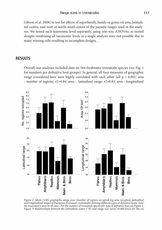
117Range sizes in trematodes
Gibson et al. 2008) to test for effects of superfamily, family or genus on area, latitudi-nal centre, east-west or north-south extent of the parasite ranges used in the analy-ses. We tested each taxonomic level separately, using one-way ANOVAs, as nested designs combining all taxonomic levels in a single analysis were not possible due to many missing cells resulting in incomplete designs.
RESULTS
Overall, our analyses included data on 564 freshwater trematode species (see Fig. 1 for numbers per definitive host groups). In general, all four measures of geographic range considered here were highly correlated with each other (all p < 0.001; area - number of regions: r2=0.84; area – latitudinal range: r2=0.83; area - longitudinal
FishAmphibians
ReptilesMammals
BirdsMammalsBirds
40
44
48
52
56
60
64
rang
e lo
ng
FishAmphibians
ReptilesMammals
BirdsMammalsBirds
4.5
5.0
5.5
6.0
6.5
7.0
7.5
8.08.5
no s
ites
No.
regi
ons
occu
pied
FishAmphibians
ReptilesMammals
BirdsMammalsBirds
2.4
2.8
3.2
3.6
4.0
4.4
4.8
area
Are
a 10
6km
2
FishAmphibians
ReptilesMammals
BirdsMammalsBirds
14
16
18
20
22
24
rang
e la
tLa
titud
inal
rang
e
Long
itudi
nal r
ange
Fish
es
Am
phib
ians
Rep
tiles
Mam
mal
s
Mam
. & B
irds
Bird
s
Fish
es
Am
phib
ians
Rep
tiles
Mam
mal
s
Mam
. & B
irds
Bird
sFishAmphibians
ReptilesMammals
BirdsMammalsBirds
40
44
48
52
56
60
64
rang
e lo
ng
FishAmphibians
ReptilesMammals
BirdsMammalsBirds
4.5
5.0
5.5
6.0
6.5
7.0
7.5
8.08.5
no s
ites
No.
regi
ons
occu
pied
FishAmphibians
ReptilesMammals
BirdsMammalsBirds
2.4
2.8
3.2
3.6
4.0
4.4
4.8
area
Are
a 10
6km
2
FishAmphibians
ReptilesMammals
BirdsMammalsBirds
14
16
18
20
22
24
rang
e la
tLa
titud
inal
rang
e
Long
itudi
nal r
ange
Fish
es
Am
phib
ians
Rep
tiles
Mam
mal
s
Mam
. & B
irds
Bird
s
Fish
es
Am
phib
ians
Rep
tiles
Mam
mal
s
Mam
. & B
irds
Bird
s
Figure 2: Mean (+SE) geographic range sizes (number of regions occupied, log area occupied, latitudinal and longitudinal range) of European freshwater trematodes utilising different types of definitive hosts. Note the truncated y-axes in all cases. For the number of trematode species per type of definitive host see Figure 1.Figure 3: Relationships between the latitudinal centre (˚N) and range size (area*10.000 km2) for the six

118118
range: r2=0.77; number of regions - latitudinal range: r2=0.70; number of regions - longitudinal range: r2=0.71; latitudinal range - longitudinal range: r2=0.77).
The species-range size distributions showed that most trematode species occupy only a few bioregions (Fig. 1). Overall, this pattern was less clear in trematodes of definitive host groups for which only limited numbers of parasite species are available (reptiles, birds & mammals, Fig. 1). In general, the range size distributions among host groups were similar, with trematodes from none of the definitive host groups having particularly large ranges. This was reflected in the mean geographic range siz-es or dimensions of trematode species among the different types of definitive hosts. Although trematode species utilising mammals or birds as definitive hosts had the smallest geographic ranges (Fig. 2), the difference was not or only marginally signifi-cant, depending on the measure of range size used (ANOVAs: Area: F5,558= 1.66, p= 0.14; number of regions: F5,558= 2.59, p= 0.02; latitudinal range: F5,558= 2.34, p= 0.04; longitudinal range: F5,558= 1.92, p= 0.09). Subsequent post-hoc compari-sons in the two significant ANOVAs showed no significant differences among any of the different comparisons (in all comparisons p≥0.53 (number of regions) or p≥0.47 (latitudinal range)).
groups of definitive hosts showing values for each trematode species (black points). Black lines indicate the observed relationships fitted from these points (area vs. linear and squared term of latitudinal centre; reptiles: area vs. linear term of latitudinal centre only). Grey lines indicate the relationships rendered by the null model simulations, based on slopes and intercepts from 1000 simulations (straight line) and the according 95% confidence intervals (For values of observed and simulated slopes and intercepts, see Table S1 in the supplementary material). Figure 4: Relationships between the latitudinal centre (˚N) and range size (area*10.000 km2) for the six

119Range sizes in trematodes
We found the relationship between latitudinal centre and area to be hump-shaped in all host groups except for reptiles, for which it was linear (Fig. 3 & 4). The linearity of the relationship for reptiles may arise because only a part of the latitudinal gradi-ent is realized: no trematode species are associated with reptiles above 55° N (Fig. 3 upper left). Both the regression analyses and the Rohde plots showed that most of the variation falls within the expectations due to geometric constraints. However, com-paring observed and simulated values, most observed relationships are steeper than expected from the null model simulations. This is also indicated by the differences in the slopes and intercepts between observed and simulated relationships.
Trematodes in all six types of definitive hosts showed similar trends in the shape of their ranges. All ranges tended to stretch more in east-west than in north-south directions (Fig. 5), as the vast majority of points fall below the diagonal line indicat-ing equal north-south and east-west extents. Furthermore, most of the points also fall below the lines indicating the pattern expected from the null models – most spe-cies have range shapes that stretch even more towards east-west vs. north-south than expected given the geographic extent and shape of the European continent and the biogeographic regions (Fig. 5).
groups of definitive hosts using Rohde plots. Black points are the mean values of log10(area), calculated from those species whose latitudinal centres fall within latitudinal bands of 3° width. Error bars indicate the standard errors of the mean. Grey lines indicate the values rendered by the null model simulations (straight line) and their respective 95% confidence intervals (dashed lines). For the number of trematode species per type of definitive host see Fig. 1. For details on null model setup, see text.
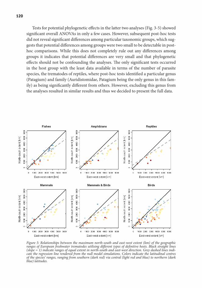
120120
Tests for potential phylogenetic effects in the latter two analyses (Fig. 3-5) showed significant overall ANOVAs in only a few cases. However, subsequent post-hoc tests did not reveal significant differences among particular taxonomic groups, which sug-gests that potential differences among groups were two small to be detectable in post-hoc comparisons. While this does not completely rule out any differences among groups it indicates that potential differences are very small and that phylogenetic effects should not be confounding the analyses. The only significant tests occurred in the host group with the least data available in terms of the number of parasite species, the trematodes of reptiles, where post-hoc tests identified a particular genus (Patagium) and family (Auridistomidae, Patagium being the only genus in this fam-ily) as being significantly different from others. However, excluding this genus from the analyses resulted in similar results and thus we decided to present the full data.
Figure 5: Relationships between the maximum north-south and east-west extent (km) of the geographic ranges of European freshwater trematodes utilising different types of definitive hosts. Black straight lines (slope = 1) indicate ranges of equal extent in north-south and east-west direction. Grey dashed lines indi-cate the regression line rendered from the null model simulations. Colors indicate the latitudinal centres of the species’ ranges, ranging from southern (dark red) via central (light red and blue) to northern (dark blue) latitudes.

121Range sizes in trematodes
DISCUSSION
The geographic range sizes of parasites in all definitive host groups showed the typi-cal right-skewed pattern observed in free-living species: most parasite species oc-cupy small ranges, and only a few species occupy large ones. The range size measures for each parasite species are likely to be overestimates as parasite species occurring within a bioregion do not necessarily occur everywhere within this region. This may particularly affect the range size measures of parasites occurring in large regions as it results in large total range sizes. However, the number of regions occupied should be the least problematic measure in this respect and thus the general trend of a right-skewed pattern seems to be robust. Fleas (Siphonaptera) ectoparasitic on small mam-mals show a similar pattern (Krasnov et al. 2005) and their geographic range size is negatively correlated with their degree of host specificity: generalist flea species, infecting a wide range of host species, had larger ranges than highly specific spe-cies (Krasnov et al. 2005). Host specificity may also underlie the pattern observed in European trematode species, although we cannot test this formally as no informa-tion on host specificity is currently available. The extreme right skew of trematode range sizes might suggest that the majority of trematodes are relatively host specific and analyses of regional parasite faunas of vertebrates indicate that the majority of helminth species are indeed relatively host specific (Gregory et al. 1991, Poulin 1992, Poulin 2007).
Being restricted to a single or just a few host species means that the spatial dis-tribution of a parasite species strongly depends on the dispersal capacities of its par-ticular host species. Dispersal capacity is probably limited in the majority of potential hosts as vertebrates also generally show hollow curve distributions of their geograph-ic range sizes (Gaston 2003). Hence, the dispersal potential of parasites should be limited by that of their hosts, and consequently their geographic ranges have to be relatively small in the majority of cases, resulting in the observed hollow curve shapes for the frequency distributions of their geographic range sizes. Dispersal limitations of the intermediate hosts involved in the complex life cycles of trematodes might further restrict the parasites’ dispersal. Host specificity is universally high for the first intermediate (mostly gastropods) host (Galaktionov and Dobrovolskij 2003) and gastropods are usually restricted in their dispersal capacity as adults (planktonic stages are not infected).
Contrary to expectation, parasites utilizing host groups presumed to have high dispersal capacities, like birds, did not have, on average, larger range sizes than those utilizing host groups with smaller dispersal capacity. Of course, the resolution of the available data might have been too coarse to detect any differences. However, con-sidering the well known importance of definitive host type for parasite dispersal, we would have expected strong differences among groups well exceeding the resolution of our data. For example, findings from parasite community structure in fish hosts

122122
on local scales indicate the dispersal capacity of the definitive host to be crucially important for parasite dispersal (Esch et al. 1988). In addition, phylogeographic evi-dence suggests that parasites using birds should achieve a greater geographic range (especially considering the large migrations of water birds in Europe). Typically, freshwater parasites using fish as definitive hosts show pronounced genetic structure among different populations on a scale of a few hundred kilometres, whereas those using birds do not, suggesting that the latter have much greater dispersal potential (Criscione and Blouin 2004). Perhaps the structuring forces acting on local scales are overcome by other forces on regional to continental scales as used in our analysis. Several non-exclusive mechanisms might be at work on these larger spatial scales. For instance, hosts with a high dispersal capacity may often also carry a high number of parasite species, as the number of parasite species exploiting a particular host spe-cies increases with that host’s geographic range size (Dritschilo et al. 1979, Gregory 1990, Shenbrot el al. 2007). Hence, a few highly mobile and widely distributed host species (e.g. migratory fish) might distribute many parasite species on a large spatial scale, although the host group in general (e.g. fish) has a relatively small dispersal capacity. In addition, the actual infection levels (e.g. prevalence, or percentage of hosts infected) of parasite species in host populations may be of importance. Inter-estingly, mean helminth prevalence in fish hosts, i.e. the proportion of individual hosts in a population that are infected, seem to be higher than in bird hosts based on comprehensive compilations of published data (Poulin 1998a,b). Hence, the higher dispersal capacity of birds might be offset by their relatively low levels of infection, decreasing the chances for a parasite species to disperse. Another mechanism blur-ring the expected pattern could be that there are simply more specialist parasites using birds compared to those using fish. These specialists would be confined to the dispersal ranges of their single definitive hosts, most of which would have limited dispersal capacity themselves as suggested by small ranges, and this may again offset any advantage associated with the high dispersal capacity of the host group in gen-eral. However, consistent comparative data from the different host groups are not available to test these ideas.
Regression analyses and Rohde plots showed that the relationship between latitu-dinal centre and range size was hump-shaped in all host groups (except for reptiles). We acknowledge that both of these methods have their pitfalls and that the coarse resolution of the data limits the analyses. Also, using latitude alone does not allow identifying underlying structuring environmental factors like climate (Hawkins and Diniz-Filho 2004). However, we think that the data are still valuable for a simple analysis of latitudinal patterns; especially since such patterns have never been stud-ied in endoparasites before. Should more detailed distributional data become avail-able in the future, more elaborate and detailed analyses will be feasible, expanding on our basic findings. However, the graphs suggest that latitude does not seem to have an important effect on range size patterns as most of the variation falls within the expectations given by the null models. Hence, the pattern arises due to the geo-

123Range sizes in trematodes
graphic shape and extent of the European continent and the biogeographic regions, with land masses being interrupted along a latitudinal band by the Mediterranean Sea in the south. Species with the mid-point of their range in the south may thus have a restricted dispersal capacity simply due to the geographical topology. In addi-tion, mid-domain effects due to the geographic extent of the continent and the biore-gions probably add to the phenomenon (Colwell and Hurtt 1994, Colwell and Lees 2000, Colwell et al. 2004). However, although the latitudinal distribution of range size largely followed the expectations from the null models, most host groups showed somewhat steeper slopes in the observed values versus the null model simulations. This might indicate that other factors besides non-biological domain effects addi-tionally mediate the latitudinal distribution of range sizes. For example, host spe-cificity may play a role in that generalist trematodes may occur in more regions than null models suggest because a higher number of potential hosts should translate into a higher dispersal capacity (see above).
The pattern of range sizes stretching more in east-west than in north-south direc-tions remained after controlling for geometric constraints of the study area with null models and is similar to the one observed in European birds (Brown and Maurer 1989). If the orientation of ranges was only determined by the shape of Europe, we would expect the data to follow the null model expectations. However, the orienta-tion is longer in the East-West direction than expected, which is probably an effect of the orientation of major climatic zones and major topographical features like moun-tain chains (e.g. the Alps), which run in an east-west direction in Europe (Brown and Maurer 1989). They act as a dispersal barrier for both free-living and parasite species. Interestingly, the effect in our data was most pronounced in trematodes with centres of distribution in the south to mid Europe. This probably points to the par-ticular importance of the southern mountain chains like the Alps and Pyrenees as biogeographic barriers for hosts and parasites. In contrast, the pattern was more or less absent in trematode species with northern distributional centres. This may be interpreted as a legacy of the ice ages with highly dispersive northern species re-colonising large parts of northern Europe after a large-scale eradication of northern faunas (Hof et al. 2008).
Any large scale analysis of geographical patterns depends on the quality of the underlying data. As discussed above, the coarse resolution of the data might be of particular concern. However, we think using these data is valid considering that the simple biogeographic patterns we investigate should not be too sensitive in this re-spect (see above) and considering that such patterns have never been investigated in endoparasites before. There are certainly data sets of better quality but for trematodes this data base is probably as good as it can get. Hence, we believe the data presented make a valuable start to investigate biodiversity patterns in this group. Other critical issues with the data set might be sampling effort and synonyms. Potential differences in sampling effort among bioregions could affect our measures of trematode range sizes. However, the trematode fauna of Europe is probably one of the best known

124124
in the world, and it has been the focus of much interest, particularly with respect to vertebrates, for a very long time. In addition, a quantitative analysis of the proportion of singletons per bioregion (species present in a single bioregion only) shows a rela-tively even distribution of singletons among bioregions (Thieltges et al. in prep.). As singletons can be good indicators of sampling effort (Novotny and Basset 2000), this suggests that sampling effort is relatively uniform among the 25 bioregions and thus not confounding our study. Synonyms among the named parasite species in the data set might be problematic but the original data set was compiled by experts in their field and therefore the nomenclature should be consistent across the bioregions. It is also difficult to see how the spatial distribution of synonymous species could occur in a way that leads to the patterns observed in our analyses. Hence, we think the data set and our analyses are sufficiently robust to test for the observed patterns.
In conclusion, the geographic range size patterns of European freshwater trema-todes show a typical hollow curve distribution, with most species having small ranges. Interestingly, varying within-range dispersal capacity among host groups (e.g. high in birds and low in fish) did not affect the range sizes of parasites, suggesting that the dispersal capacity of definitive hosts is of much less importance on large spatial scales than small-scale studies have suggested. Range sizes of trematodes showed a hump-shaped distribution along a latitudinal gradient similar to null model expecta-tions, suggesting that the observed pattern is caused by the extent and shape of the geographic domain and that no latitudinal trend exists. Finally, trematode ranges tended to stretch more in east-west than in north-south directions, even when the geographic domain was considered by null models, pointing to geographic features like the Alps as major barriers for the dispersal of parasites. Our analysis was con-fined to trematodes and it will be interesting in futures studies to investigate other parasite groups (e.g. cestodes, nematodes, ectoparasites etc.) to see if the patterns hold true more generally.
ACKNOWLEDGEMENTS
DWT acknowledges support by a fellowship from the German Research Founda-tion (DFG) (Th 1361/1-1). CH and MKB acknowledge the Danish National Research Foundation for its support of the Danish Center for Macroecology, Evolution and Climate. We thank the reviewers for their help in improving the manuscript.
125Range sizes in trematodes
REFERENCES
Anderson, S. 1977. Geographic ranges of North American terrestrial mammals. - Am. Mus. Novitates 2629: 1-15.
Anderson, S. 1984a. Geographic ranges of North American birds. - Am. Mus. Novitates 2785: 1-17.
Anderson, S. 1984b. Areography of North American fishes, amphibians and reptiles. - Am. Mus. Novitates 2802: 1-6.
Anderson, S. and Marcus, L.F. 1992. Areography of Australian tetrapods. - Austral. J. Zool. 40: 627-651.
Brändle, M. and Brandl, R. 2001. Species richness of insects and mites on trees: expanding Southwood. - J. Anim. Ecol. 70: 491-504.
Brooks, T. et al. 2001. Toward a blueprint for conservation in Africa. - BioScience 51: 613-624.
Brown, J.H. 1984 On the relationship between abundance and distribution of species. - Am. Nat. 124: 255-279.
Brown, J.H. 1995. Macroecology. University of Chicago Press.
Brown, J.H. and Maurer, B.A. 1989. Macroecology: the division of food and space among spe-cies on continents. - Science 243: 1145-1150.
Brown, J.H. et al. 1996. The geographic range: size, shape, boundaries and internal structure. - Ann. Rev. Ecol. Syst. 27: 597-623.
Colwell, R.K. and Hurtt, G.C. 1994. Nonbiological gradients in species richness and a spurious Rapoport effect. - Am. Nat. 144: 570–595.
Colwell, R.K. and Lees, D.C. 2000. The mid-domain effect: geometric constraints on the geogra-phy of species richness. - Trends Ecol. Evol. 15: 70-76.
Colwell. R.K. et al. 2004. The mid-domain effect and species richness patterns: what have we learned so far? - Am. Nat. 163: E1-E23
Criscione, C.D. and Blouin, M.S. 2004. Life cycles shape parasite evolution: comparative popu-lation genetics of salmon trematodes. - Evolution 58: 198-202.
Dritschilo, W. et al. 1975. Insular biogeography: of mice and mites. - Science 190: 467-469.
Esch, G.W. et al. 1988. Patterns in helminth communities in freshwater fish in Great Britain: alternative strategies for colonization. - Parasitology 96: 519-532.
Galaktionov, K.V. and Dobrovolskij, A.A. 2003. The biology and evolution of trematodes: an essay on the morphology, life cycles, transmission, and evolution of digenetic trematodes. Kluwer Academic Publisher.
Gaston, K.J. 2003. The structure and dynamics of geographic ranges. Oxford University Press.
Gaston, K.J. et al. 1998. Rapoport’s rule: time for an epitaph? - Trends Ecol. Evol. 13: 70-74.
Gibson, D.I. et al. (eds) (2008) Keys to the Trematoda. Vol. 3. CAB International.
Gibson, D.I. et al. (eds) (2002) Keys to the Trematoda. Vol. 1. CAB International.

126
Graves, G. R. 1985. Elevational correlates of speciation and intraspecific geographic-variation in plumage in andean forest birds. — Auk 102: 556-579.
Gregory, R.D. 1990. Parasites and host geographic range as illustrated by waterfowl. - Funct. Ecol. 4: 645-654.
Gregory, R.D. et al. 1991. Life history, ecology and parasite community structure in Soviet birds. - Biol. J. Linn Soc. 43: 249-262.
Griffiths, D. 2006. Pattern and process in the ecological biogeography of European freshwater fish. - J. Anim. Ecol. 75: 734–751.
Hewitt, G.M. 1999. Post-glacial re-colonazation of European biota. - J. Linn Soc. 68: 87-112.
Hof, C. et al. 2008. Latitudinal variation of diversity in European freshwater animals is not con-cordant across habiat types. - Global Ecol. Biogeogr. 17: 539-546.
Illies, J. 1978. Limnofauna Europaea, 2nd edn. Gustav Fischer Verlag, Stuttgart.
Jetz, W. and Rahbek, C. 2001. Geometric constraints explain much of the species richness pat-tern in african birds. — Proceedings of the National Academy of Sciences of the United States of America 98: 5661-5666.
Jones, A. et al. (eds) 2005. Keys to the Trematoda. Vol. 2. CAB International
Krasnov, B.R. et al. 2005. Host specificity and geographic range in haematophagous ectopara-sites. - Oikos 108: 449-456.
Krasnov, B.R. et al. 2004. Flea species richness and parameters of host body, host geography and host ‘milieu’. - J. Anim. Ecol. 73: 1121-1128.
Krasnov, B.R. et al. 2008. Latitudinal gradients in niche breadth: empirical evidence from hae-matophagous ectoparasites. - J. Biogeogr. 35: 592-601.
Letcher, A.J. and Harvey, P.H. 1994. Variation in geographic range size among mammals of the Palearctic. - Am. Nat. 144: 30-42.
MacDonald, G.M. 2003. Biogeography: space, time, and life. Wiley.
Novotny V. and Basset, Y. 2000. Rare species in communities of tropical insect herbivores: pon-dering the mystery of singletons. - Oikos 89: 564–572.
Poulin, R. 1992. Determinants of host-specificity in parasites of freshwater fishes. - Int. J. Para-sitol. 22: 753-758.
Poulin, R. 1998a. Large-scale patterns of host use by parasites of freshwater fish. - Ecol. Letters 1: 118-128.
Poulin, R. 1998b. Comparison of three estimators of species richness in parasite component communities. - J. Parasitol. 84: 485-490.
Poulin, R. 2007. Evolutionary ecology of parasites. Princeton University Press.
Rapoport, E.H. 1982. Areography: geographical strategies of species. Pergamon.
Rohde, K. et al. 1993. Rapoport’s rule does not apply to marine teleosts and cannot explain lati-tudinal gradients in species richness. - Am. Nat. 142: 1-16.
Rohde, K. 1993. Ecology of marine parasites: an introduction to marine parasitology. CAB In-ternational.

127Range sizes in trematodes
Rohde, K. 1996. Rapoport’s rule is a local phenomenon and cannot explain latitudinal gradients in species richness. - Biodiv. Letters 3: 10-13.
Shenbrot, G. et al. (2007) Geographical range size and host specificity in ectoparasites: a case study with Amphisylla fleas and rodent hosts. - J. Biogeogr. 34: 1679–1690.
Stevens, G.C. 1989. The latitudinal gradient in geographical range: how so many species co-exist in the tropics. - Am. Nat. 133: 240-25.
Willis, J.C. 1922. Age and area. Cambridge University Press.

128128

Published as:Nachman, G. N. and Borregaard, M. K. 2010. From complex spatial
dynamics to simple Markov chain models: do predators and prey leave footprints?
Ecography 33: 137-147
Appendix II:From complex spatial dynamics to
simple Markov chain models: do predators and prey leave footprints?

130
From complex spatial dynamics to simple Markov chain models:do predators and prey leave footprints?
Gosta Nachman and Michael K. Borregaard
G. Nachman ([email protected]) and M. K. Borregaard, Section of Ecology and Evolution, Dept of Biology, Univ. of Copenhagen,Universitetsparken 15, DK 2100 Copenhagen Ø, Denmark.
In this paper we present a concept for using presence�absence data to recover information on the population dynamics ofpredator�prey systems. We use a highly complex and spatially explicit simulation model of a predator�prey mite systemto generate simple presence�absence data: the number of patches with both prey and predators, with prey only, withpredators only, and with neither species, along with the number of patches that change from one state to another in eachtime step. The average number of patches in the four states, as well as the average transition probabilities from one state toanother, are then depicted in a state transition diagram, constituting the ‘‘footprints’’ of the underlying populationdynamics. We investigate to what extent changes in the population processes modeled in the complex simulation (i.e. thepredator’s functional response and the dispersal rates of both species) are reflected by different footprints.The transition probabilities can be used to forecast the expected fate of a system given its current state. However, the
transition probabilities in the modeled system depend on the number of patches in each state. We develop a model for thedependence of transition probabilities on state variables, and combine this information in a Markov chain transitionmatrix model. Finally, we use this extended model to predict the long-term dynamics of the system and to reveal itsasymptotic steady state properties.
The simplest models of predator�prey systems, such as theLotka-Volterra model (cf. Lotka 1925), describe populationdynamics by means of only two variables: the meandensities of prey and predators. Changes in the density ofone species are linked to changes in the other through thefunctional response (Solomon 1949), which predicts howmany prey individuals a predator consumes per time unit ata given mean prey density. However, if prey and predatorsare not evenly distributed in space, mean densities alone arelikely to be poor predictors of predation rates, because theyprovide no information about the actual degree of spatialoverlap between the species (Nachman 2006a, b).
Spatially explicit population models (Gurney et al.1998), on the other hand, apply information about thenumbers of prey and predators occupying every spatial unit(called patches) within a system. The changes in populationsizes within each patch due to births, deaths, immigrationsand emigrations can then be computed for each small timestep. These models are powerful strategic tools for under-standing predator�prey dynamics, because they generatedetailed predictions of the system’s trajectory through time.However, spatially explicit models need to be fed by highresolution data about the current distributions of thespecies, which limits their practical application for e.g.pest management or conservation. A solution in these casesis to develop spatially implicit models that only need low
resolution data easily obtainable from field samples, as e.g.proportion of plants or leaves with or without prey andpredators, but still retain enough complexity to generaterealistic predictions.
In this paper, we model the dynamics of an acarinepredator�prey system consisting of the two-spotted spidermite Tetranychus urticae and its phytoseiid predatorPhytoseiulus persimilis. The spider mite is a serious pest inmany crops, including greenhouse cucumbers. The predatorspecies is known as a very efficient predator of T. urticaeand therefore widely used as a biocontrol agent against it(Helle and Sabelis 1985).
We use a spatially explicit stochastic simulation model ofthe above system to produce spatio-temporal patterns ofprey and predators. The output of these simulations formsthe basis for developing a spatially implicit matrix model.The advantage of using model-simulated data instead offield-collected data is that we are in control of the processesthat produce the observed predator�prey dynamics. Thismeans that we can test the hypothesis that these underlyingprocesses are revealed by the parameters of the matrixmodel. Specifically, we address the hypothesis that thetransition probabilities reflect the dispersal ability of bothspecies and the efficacy of the predators. If this hypothesis isconfirmed, transition probabilities and steady state distribu-tions, which can be combined and depicted graphically as a
Ecography 33: 137�147, 2010doi: 10.1111/j.1600-0587.2009.06045.x
# 2010 The Authors. Journal compilation # 2010 Ecography
Subject Editors: Joaquin Hortal and Carsten Rahbek. Accepted 24 September 2009
137
SPEC
IA
LISSU
E
131
From complex spatial dynamics to simple Markov chain models:do predators and prey leave footprints?
Gosta Nachman and Michael K. Borregaard
G. Nachman ([email protected]) and M. K. Borregaard, Section of Ecology and Evolution, Dept of Biology, Univ. of Copenhagen,Universitetsparken 15, DK 2100 Copenhagen Ø, Denmark.
In this paper we present a concept for using presence�absence data to recover information on the population dynamics ofpredator�prey systems. We use a highly complex and spatially explicit simulation model of a predator�prey mite systemto generate simple presence�absence data: the number of patches with both prey and predators, with prey only, withpredators only, and with neither species, along with the number of patches that change from one state to another in eachtime step. The average number of patches in the four states, as well as the average transition probabilities from one state toanother, are then depicted in a state transition diagram, constituting the ‘‘footprints’’ of the underlying populationdynamics. We investigate to what extent changes in the population processes modeled in the complex simulation (i.e. thepredator’s functional response and the dispersal rates of both species) are reflected by different footprints.The transition probabilities can be used to forecast the expected fate of a system given its current state. However, the
transition probabilities in the modeled system depend on the number of patches in each state. We develop a model for thedependence of transition probabilities on state variables, and combine this information in a Markov chain transitionmatrix model. Finally, we use this extended model to predict the long-term dynamics of the system and to reveal itsasymptotic steady state properties.
The simplest models of predator�prey systems, such as theLotka-Volterra model (cf. Lotka 1925), describe populationdynamics by means of only two variables: the meandensities of prey and predators. Changes in the density ofone species are linked to changes in the other through thefunctional response (Solomon 1949), which predicts howmany prey individuals a predator consumes per time unit ata given mean prey density. However, if prey and predatorsare not evenly distributed in space, mean densities alone arelikely to be poor predictors of predation rates, because theyprovide no information about the actual degree of spatialoverlap between the species (Nachman 2006a, b).
Spatially explicit population models (Gurney et al.1998), on the other hand, apply information about thenumbers of prey and predators occupying every spatial unit(called patches) within a system. The changes in populationsizes within each patch due to births, deaths, immigrationsand emigrations can then be computed for each small timestep. These models are powerful strategic tools for under-standing predator�prey dynamics, because they generatedetailed predictions of the system’s trajectory through time.However, spatially explicit models need to be fed by highresolution data about the current distributions of thespecies, which limits their practical application for e.g.pest management or conservation. A solution in these casesis to develop spatially implicit models that only need low
resolution data easily obtainable from field samples, as e.g.proportion of plants or leaves with or without prey andpredators, but still retain enough complexity to generaterealistic predictions.
In this paper, we model the dynamics of an acarinepredator�prey system consisting of the two-spotted spidermite Tetranychus urticae and its phytoseiid predatorPhytoseiulus persimilis. The spider mite is a serious pest inmany crops, including greenhouse cucumbers. The predatorspecies is known as a very efficient predator of T. urticaeand therefore widely used as a biocontrol agent against it(Helle and Sabelis 1985).
We use a spatially explicit stochastic simulation model ofthe above system to produce spatio-temporal patterns ofprey and predators. The output of these simulations formsthe basis for developing a spatially implicit matrix model.The advantage of using model-simulated data instead offield-collected data is that we are in control of the processesthat produce the observed predator�prey dynamics. Thismeans that we can test the hypothesis that these underlyingprocesses are revealed by the parameters of the matrixmodel. Specifically, we address the hypothesis that thetransition probabilities reflect the dispersal ability of bothspecies and the efficacy of the predators. If this hypothesis isconfirmed, transition probabilities and steady state distribu-tions, which can be combined and depicted graphically as a
Ecography 33: 137�147, 2010doi: 10.1111/j.1600-0587.2009.06045.x
# 2010 The Authors. Journal compilation # 2010 Ecography
Subject Editors: Joaquin Hortal and Carsten Rahbek. Accepted 24 September 2009
137
SPEC
IA
LISSU
E

132
‘‘footprint’’ diagram, may serve as a diagnostic tool underfield conditions, with application for e.g. pest control.
The spatially implicit model is based on a model byMaynard Smith (1974), who simplified predator�preydynamics by dividing patches into a set of categories: empty,inhabited by few individuals (of prey and/or predators), orinhabited by many individuals. Gurney and Nisbet (1978)simplified this classification further to just four groups:patches with both prey and predators, with prey only, withpredators only, and empty patches. Over a certain timeinterval patches are likely to change from one state toanother. The likelihood of such discrete events can beexpressed through transition probabilities, which are ele-ments of a finite Markov chain model and are defined by atransition matrix (Dharmadhikari 1963). Once the elementsof the transition matrix and the current state of the system areknown, it is straightforward to calculate the expected state ofthe system after one time step, and to do this recurrently forany desired number of time steps. Matrix transition models(also called population projection matrices) are useful asanalytical and predictive tools in e.g. conservation (Lusseau2003), landscape management (Yemshanov and Perera2002) and pest control strategies (Woolhouse and Harmsen1991).
A challenge for applying matrix models to predator�preysystems is that the transition probabilities are likely to benon-stationary, i.e. to depend on the number of patches ineach state; e.g. if there are many patches already containingprey, it is more likely that an empty patch will be occupiedby prey in the next time step (Gurney and Nisbet 1978,Woolhouse and Harmsen 1987a, b). We apply a correla-tion-based approach to identify simple functional relation-ships between the state variables and the transitionprobabilities and use simulated data to parameterize theserelationships. The resulting projection matrix can be used topredict the system’s asymptotic behaviour in order toinvestigate emergent properties such as stability, bifurca-tions, sensitivity etc. (Caswell 2001).
Methods
The biological system
As the biological background for modeling, we used a seriesof experiments conducted in 500m2 commercial green-houses (Nachman 1981). Each greenhouse hosted 720cucumber plants arranged in 8 rows. Early in the growingseason every second plant in the greenhouses were inocu-lated with five or six adult female spider mites and two dayslater two, three or four adult female predators were releasedonto the same plants. The plants were sampled every weekduring the following 23 weeks. At each sampling occasion36 plants were randomly selected and three leaves werepicked from each. All mites occurring on their lower leafsurface were counted. Details on the biology of the involvedspecies can be found elsewhere (Helle and Sabelis 1985).
The simulation model
The complex simulation model used to simulate the green-house system and to parameterize the transition matrices
is described in Nachman (2001). Basically the modelapplies a metapopulation concept where each plant in agreenhouse is considered as a patch with its own localdynamics. In contrast to the classic metapopulationapproach (Levins 1969), the model is spatially explicitwith respect to patch location. Furthermore, patches arecharacterized by their size/quality and the numbers ofindividuals present. Finally, dispersal from a patch iscondition-dependent and the likelihood that an individualsucceeds to move from one patch to another depends on thedistance between them. The model incorporates demo-graphic stochasticity to cope with discrete events as births,deaths, immigrations and emigrations; this stochasticityplays an important role in creating patch asynchrony(Nachman 1987a, b). Sex and age structure of the popula-tions are modeled implicitly by using weighted parametervalues. The model is implemented in Delphi 7 (Borland).
The model described in Nachman (2001) appliedHolling’s (1959) disc equation to model the functionalresponse of P. persimilis. Since this model assumes that thepredators search for prey at random, it is unrealistic whenthe prey is patchily distributed and the predators exert non-random search (Nachman 2006a). The problem was partlyalleviated in Nachman (2001) by increasing the parameterexpressing the predator’s attack efficiency, but since then amore mechanistic functional response model has beenproposed (Nachman 2006b). It incorporates the spatialdistribution of the prey among leaves within plants, theaggregative response of the predators to the prey distribu-tion and mutual interference among searching predators.This new model was chosen to represent the functionalresponse of P. persimilis in the simulations.
The simulations
The model simulated a greenhouse system consisting of 400fully grown plants arranged in 8 rows. The distances betweenplants and the physical conditions were assumed to be thesame as those described in Nachman (2001). At day 0, everysecond plant was inoculated with 60 spider mites, and twodays later the same plants were inoculated with 3 predatorymites. The duration of a simulation was set to 3000 d.Provided both mite species were still present in the system atthe end of a simulation, the last 2000 d were used for thesubsequent analyses. For each of the 2000 d, the followinginformation was recorded: average number of prey andpredators per plant, the number of plants without mites, withboth species, with prey only and with predators only, and thenumber of transitions from one state to another during thepreceding day. The growing season for greenhouse cucum-bers is normally ca 200 d, but since we were interested in thelong term dynamics of prey and predators, it was necessary toassume that the plants do not deteriorate for reasons otherthan exploitation by the spider mites, and that they are able torecover from any level of damage; though the time to recovercompletely increases with the severity of the damage. Thisassumption also facilitates generalization to other multi-patch systems, where the level of biological patch deteriora-tion is often negligible.
The model was used to simulate six different scenarios:Scenario 1: the prey is patchily distributed among leaves
138
SPEC
IA
LISSU
E
within plants and the predators search non-randomly. Thisscenario served as the standard case against which the otherfive scenarios were compared. The simulations were basedon the default parameter values in Nachman (2001,2006b). Scenario 2: the prey is distributed as in Scenario1, but the predators exhibit random search. Since it turnedout that a randomly searching predator performed so poorlythat it could not obtain sufficient prey for its survival, weassumed that low predation efficiency is partly compensatedby a better ability to exploit consumed prey. This wasachieved by doubling the per capita birth rate and halvingthe per capita death rate compared with the predator inScenario 1. Scenario 3: as Scenario 1 except that the prey isevenly distributed among leaves within plants. Scenario 4:as Scenario 1 except that the dispersal rate of the prey isreduced by a factor 10. Scenario 5: as Scenario 1 except thatthe dispersal rate of the predator is increased by a factor 10.Scenario 6: as Scenario 1 except that the dispersal rate of theprey is reduced by a factor 10 and the dispersal rate of thepredator is increased by a factor 10.
In order to compare the state transition diagrams (called‘‘footprints’’) originating from different scenarios, it isnecessary to compare them with the variation amongreplicates within the same scenario; this ensures that thedifferences are not just due to the inherent stochasticityassociated with the simulations. We therefore also ran sixreplicates of Scenario 1 and calculated the standard deviationof the state variables and the transition probabilities aftersubjecting the data to an arcsine square root transformation.95% confidence limits for the variables were obtained after aback transformation (Sokal and Rohlf 1995).
The matrix model
The full transition matrix can be described by consideringthat at any given time t a patch (plant) can be in one of thefour states: occupied by neither species (State 1); occupiedby prey only (State 2), occupied by both species (State 3),and occupied by predators only (State 4). The distributionof the N plants in each of the four states at time t can beexpressed as a vector with four elements Q (t )�fQ 1(t ) Q 2(t ) Q 3(t ) Q 4(t )g where Qi(t) denotes thenumber of plants in state i (i�1, 2, 3, 4). Note thata4
i�1Qi(t )�N and that a4i�1qi(t )�1; where qi is the
proportion of plants in state i, i.e. qi�Qi=N : Theprobability that a plant will be in state i at time t�1 givenit is in state j at time t (j�1, 2, 3, 4) is denoted aij. Hence,the index j represents the donor state and index i therecipient state (Caswell 2001).
The state vector Q at time t�1 can therefore be found as
Q (t�1)�
Q1(t�1)Q2(t�1)Q3(t�1)Q4(t�1)
8>><>>:
9>>=>>;
�
a11 a12 a13 a14a21 a22 a23 a24a31 a32 a33 a34a41 a42 a43 a44
8>><>>:
9>>=>>;
Q1(t )Q2(t )Q3(t )Q4(t )
8>><>>:
9>>=>>;�AQ (t )
(1)
where A is a non-negative transition matrix. The valuesof aij are constrained by aij]0 and a4
i�1aij�1 for j�1, 2,3, 4.
The transition probabilities for the time interval (t, t�1)are estimated from sampling data as
aij (t )�nij
Qj (t )(2)
where nij denotes the number of transitions from state j tostate i.
Transition probabilities depend on the time intervalsbetween successive samplings. The shorter the intervals, theless likely it will be that a patch changes to another state,and in particular that a patch passes through more than asingle state. Ideally, the system should be sampled atintervals that are so short that the likelihood that a patchundergoes more than a single transition can be ignored.This reduces the 16 elements of the full 4 times 4 transitionmatrix to (maximally) 12 non-zero elements: the probabil-ities for each of the four patch types to remain the sametype, change to the next type in the sequence, or revert tothe immediately preceding type. Because a patch is allowedto revert to the preceding type, the matrix includes morethan the eight non-zero elements employed when aunidirectional sequence is assumed. A unidirectional cyclicsequence from state 1 through state 4 and back to state 1was suggested by Gurney and Nisbet (1978) as sufficient tomodel Huffaker (1958) and Huffaker et al.’s (1963)experiments with acarine prey and predators in a patchysystem composed of oranges; however, as pointed out byWoolhouse and Harmsen (1987a), at least some of thetransitions are likely to be reversible. For instance, predatorsmay leave a patch before all prey individuals have beenconsumed or new prey individuals may move to patcheswhere only predators remain after having eradicated preyindividuals from the patch.
Test for stationarity
Time-homogeneity of the transition matrix was tested bymeans of log-linear analyses; this method is recommendedby Caswell (2001) as an alternative to the procedureproposed by Anderson and Goodman (1957). Matricesthat fail to be time-homogenous because one or more of itstransition probabilities vary with time are said to be non-stationary (Anderson and Goodman 1957). Log-linearanalysis was also applied to check the similarity of matricesobtained from replicated runs of the same model and to testwhether matrices obtained from different models differsignificantly. The log-linear analyses were carried out bymeans of PROC CATMOD in SAS Enterprise guide 4.1(SAS Inst.).
State transition diagrams
The average values of qi (t) and aij (t), recorded on a dailybasis for the last 2000 d in a simulation, were visualizedgraphically as a state transition diagram, where states arerepresented by circles with an area proportional to theaverage value of qi, and transitions are represented by arrows
139
SPEC
IA
LISSU
E

133
‘‘footprint’’ diagram, may serve as a diagnostic tool underfield conditions, with application for e.g. pest control.
The spatially implicit model is based on a model byMaynard Smith (1974), who simplified predator�preydynamics by dividing patches into a set of categories: empty,inhabited by few individuals (of prey and/or predators), orinhabited by many individuals. Gurney and Nisbet (1978)simplified this classification further to just four groups:patches with both prey and predators, with prey only, withpredators only, and empty patches. Over a certain timeinterval patches are likely to change from one state toanother. The likelihood of such discrete events can beexpressed through transition probabilities, which are ele-ments of a finite Markov chain model and are defined by atransition matrix (Dharmadhikari 1963). Once the elementsof the transition matrix and the current state of the system areknown, it is straightforward to calculate the expected state ofthe system after one time step, and to do this recurrently forany desired number of time steps. Matrix transition models(also called population projection matrices) are useful asanalytical and predictive tools in e.g. conservation (Lusseau2003), landscape management (Yemshanov and Perera2002) and pest control strategies (Woolhouse and Harmsen1991).
A challenge for applying matrix models to predator�preysystems is that the transition probabilities are likely to benon-stationary, i.e. to depend on the number of patches ineach state; e.g. if there are many patches already containingprey, it is more likely that an empty patch will be occupiedby prey in the next time step (Gurney and Nisbet 1978,Woolhouse and Harmsen 1987a, b). We apply a correla-tion-based approach to identify simple functional relation-ships between the state variables and the transitionprobabilities and use simulated data to parameterize theserelationships. The resulting projection matrix can be used topredict the system’s asymptotic behaviour in order toinvestigate emergent properties such as stability, bifurca-tions, sensitivity etc. (Caswell 2001).
Methods
The biological system
As the biological background for modeling, we used a seriesof experiments conducted in 500m2 commercial green-houses (Nachman 1981). Each greenhouse hosted 720cucumber plants arranged in 8 rows. Early in the growingseason every second plant in the greenhouses were inocu-lated with five or six adult female spider mites and two dayslater two, three or four adult female predators were releasedonto the same plants. The plants were sampled every weekduring the following 23 weeks. At each sampling occasion36 plants were randomly selected and three leaves werepicked from each. All mites occurring on their lower leafsurface were counted. Details on the biology of the involvedspecies can be found elsewhere (Helle and Sabelis 1985).
The simulation model
The complex simulation model used to simulate the green-house system and to parameterize the transition matrices
is described in Nachman (2001). Basically the modelapplies a metapopulation concept where each plant in agreenhouse is considered as a patch with its own localdynamics. In contrast to the classic metapopulationapproach (Levins 1969), the model is spatially explicitwith respect to patch location. Furthermore, patches arecharacterized by their size/quality and the numbers ofindividuals present. Finally, dispersal from a patch iscondition-dependent and the likelihood that an individualsucceeds to move from one patch to another depends on thedistance between them. The model incorporates demo-graphic stochasticity to cope with discrete events as births,deaths, immigrations and emigrations; this stochasticityplays an important role in creating patch asynchrony(Nachman 1987a, b). Sex and age structure of the popula-tions are modeled implicitly by using weighted parametervalues. The model is implemented in Delphi 7 (Borland).
The model described in Nachman (2001) appliedHolling’s (1959) disc equation to model the functionalresponse of P. persimilis. Since this model assumes that thepredators search for prey at random, it is unrealistic whenthe prey is patchily distributed and the predators exert non-random search (Nachman 2006a). The problem was partlyalleviated in Nachman (2001) by increasing the parameterexpressing the predator’s attack efficiency, but since then amore mechanistic functional response model has beenproposed (Nachman 2006b). It incorporates the spatialdistribution of the prey among leaves within plants, theaggregative response of the predators to the prey distribu-tion and mutual interference among searching predators.This new model was chosen to represent the functionalresponse of P. persimilis in the simulations.
The simulations
The model simulated a greenhouse system consisting of 400fully grown plants arranged in 8 rows. The distances betweenplants and the physical conditions were assumed to be thesame as those described in Nachman (2001). At day 0, everysecond plant was inoculated with 60 spider mites, and twodays later the same plants were inoculated with 3 predatorymites. The duration of a simulation was set to 3000 d.Provided both mite species were still present in the system atthe end of a simulation, the last 2000 d were used for thesubsequent analyses. For each of the 2000 d, the followinginformation was recorded: average number of prey andpredators per plant, the number of plants without mites, withboth species, with prey only and with predators only, and thenumber of transitions from one state to another during thepreceding day. The growing season for greenhouse cucum-bers is normally ca 200 d, but since we were interested in thelong term dynamics of prey and predators, it was necessary toassume that the plants do not deteriorate for reasons otherthan exploitation by the spider mites, and that they are able torecover from any level of damage; though the time to recovercompletely increases with the severity of the damage. Thisassumption also facilitates generalization to other multi-patch systems, where the level of biological patch deteriora-tion is often negligible.
The model was used to simulate six different scenarios:Scenario 1: the prey is patchily distributed among leaves
138
SPEC
IA
LISSU
E
within plants and the predators search non-randomly. Thisscenario served as the standard case against which the otherfive scenarios were compared. The simulations were basedon the default parameter values in Nachman (2001,2006b). Scenario 2: the prey is distributed as in Scenario1, but the predators exhibit random search. Since it turnedout that a randomly searching predator performed so poorlythat it could not obtain sufficient prey for its survival, weassumed that low predation efficiency is partly compensatedby a better ability to exploit consumed prey. This wasachieved by doubling the per capita birth rate and halvingthe per capita death rate compared with the predator inScenario 1. Scenario 3: as Scenario 1 except that the prey isevenly distributed among leaves within plants. Scenario 4:as Scenario 1 except that the dispersal rate of the prey isreduced by a factor 10. Scenario 5: as Scenario 1 except thatthe dispersal rate of the predator is increased by a factor 10.Scenario 6: as Scenario 1 except that the dispersal rate of theprey is reduced by a factor 10 and the dispersal rate of thepredator is increased by a factor 10.
In order to compare the state transition diagrams (called‘‘footprints’’) originating from different scenarios, it isnecessary to compare them with the variation amongreplicates within the same scenario; this ensures that thedifferences are not just due to the inherent stochasticityassociated with the simulations. We therefore also ran sixreplicates of Scenario 1 and calculated the standard deviationof the state variables and the transition probabilities aftersubjecting the data to an arcsine square root transformation.95% confidence limits for the variables were obtained after aback transformation (Sokal and Rohlf 1995).
The matrix model
The full transition matrix can be described by consideringthat at any given time t a patch (plant) can be in one of thefour states: occupied by neither species (State 1); occupiedby prey only (State 2), occupied by both species (State 3),and occupied by predators only (State 4). The distributionof the N plants in each of the four states at time t can beexpressed as a vector with four elements Q (t )�fQ 1(t ) Q 2(t ) Q 3(t ) Q 4(t )g where Qi(t) denotes thenumber of plants in state i (i�1, 2, 3, 4). Note thata4
i�1Qi(t )�N and that a4i�1qi(t )�1; where qi is the
proportion of plants in state i, i.e. qi�Qi=N : Theprobability that a plant will be in state i at time t�1 givenit is in state j at time t (j�1, 2, 3, 4) is denoted aij. Hence,the index j represents the donor state and index i therecipient state (Caswell 2001).
The state vector Q at time t�1 can therefore be found as
Q (t�1)�
Q1(t�1)Q2(t�1)Q3(t�1)Q4(t�1)
8>><>>:
9>>=>>;
�
a11 a12 a13 a14a21 a22 a23 a24a31 a32 a33 a34a41 a42 a43 a44
8>><>>:
9>>=>>;
Q1(t )Q2(t )Q3(t )Q4(t )
8>><>>:
9>>=>>;�AQ (t )
(1)
where A is a non-negative transition matrix. The valuesof aij are constrained by aij]0 and a4
i�1aij�1 for j�1, 2,3, 4.
The transition probabilities for the time interval (t, t�1)are estimated from sampling data as
aij (t )�nij
Qj (t )(2)
where nij denotes the number of transitions from state j tostate i.
Transition probabilities depend on the time intervalsbetween successive samplings. The shorter the intervals, theless likely it will be that a patch changes to another state,and in particular that a patch passes through more than asingle state. Ideally, the system should be sampled atintervals that are so short that the likelihood that a patchundergoes more than a single transition can be ignored.This reduces the 16 elements of the full 4 times 4 transitionmatrix to (maximally) 12 non-zero elements: the probabil-ities for each of the four patch types to remain the sametype, change to the next type in the sequence, or revert tothe immediately preceding type. Because a patch is allowedto revert to the preceding type, the matrix includes morethan the eight non-zero elements employed when aunidirectional sequence is assumed. A unidirectional cyclicsequence from state 1 through state 4 and back to state 1was suggested by Gurney and Nisbet (1978) as sufficient tomodel Huffaker (1958) and Huffaker et al.’s (1963)experiments with acarine prey and predators in a patchysystem composed of oranges; however, as pointed out byWoolhouse and Harmsen (1987a), at least some of thetransitions are likely to be reversible. For instance, predatorsmay leave a patch before all prey individuals have beenconsumed or new prey individuals may move to patcheswhere only predators remain after having eradicated preyindividuals from the patch.
Test for stationarity
Time-homogeneity of the transition matrix was tested bymeans of log-linear analyses; this method is recommendedby Caswell (2001) as an alternative to the procedureproposed by Anderson and Goodman (1957). Matricesthat fail to be time-homogenous because one or more of itstransition probabilities vary with time are said to be non-stationary (Anderson and Goodman 1957). Log-linearanalysis was also applied to check the similarity of matricesobtained from replicated runs of the same model and to testwhether matrices obtained from different models differsignificantly. The log-linear analyses were carried out bymeans of PROC CATMOD in SAS Enterprise guide 4.1(SAS Inst.).
State transition diagrams
The average values of qi (t) and aij (t), recorded on a dailybasis for the last 2000 d in a simulation, were visualizedgraphically as a state transition diagram, where states arerepresented by circles with an area proportional to theaverage value of qi, and transitions are represented by arrows
139
SPEC
IA
LISSU
E
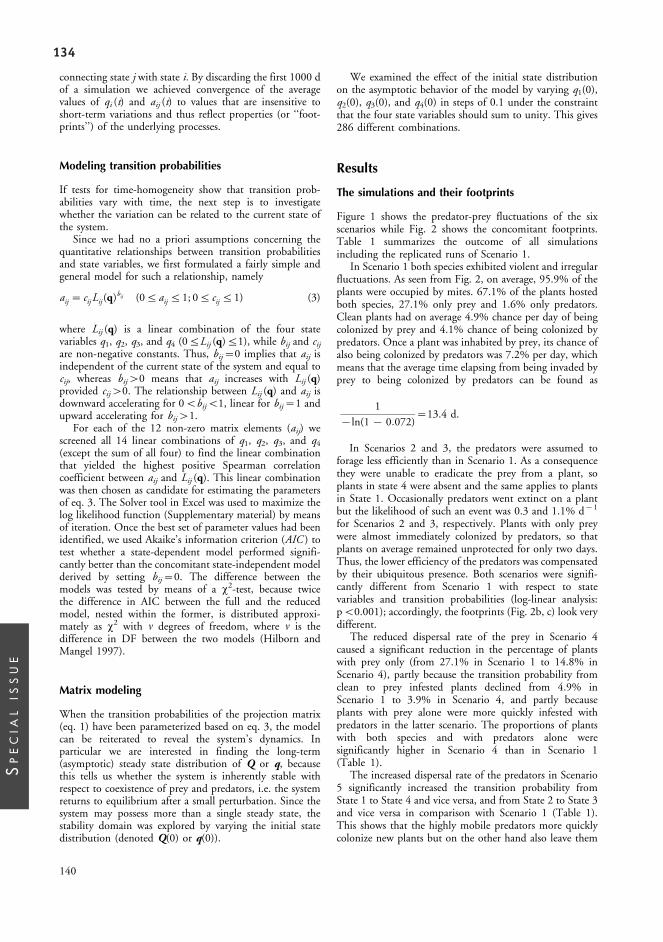
134
connecting state j with state i. By discarding the first 1000 dof a simulation we achieved convergence of the averagevalues of qi (t) and aij (t) to values that are insensitive toshort-term variations and thus reflect properties (or ‘‘foot-prints’’) of the underlying processes.
Modeling transition probabilities
If tests for time-homogeneity show that transition prob-abilities vary with time, the next step is to investigatewhether the variation can be related to the current state ofthe system.
Since we had no a priori assumptions concerning thequantitative relationships between transition probabilitiesand state variables, we first formulated a fairly simple andgeneral model for such a relationship, namely
aij� cijLij (q)bij (05aij51; 05 cij51) (3)
where Lij (q) is a linear combination of the four statevariables q1, q2, q3, and q4 (05Lij (q)51), while bij and cijare non-negative constants. Thus, bij�0 implies that aij isindependent of the current state of the system and equal tocij, whereas bij�0 means that aij increases with Lij (q)provided cij�0. The relationship between Lij (q) and aij isdownward accelerating for 0BbijB1, linear for bij�1 andupward accelerating for bij�1.
For each of the 12 non-zero matrix elements (aij) wescreened all 14 linear combinations of q1, q2, q3, and q4(except the sum of all four) to find the linear combinationthat yielded the highest positive Spearman correlationcoefficient between aij and Lij (q). This linear combinationwas then chosen as candidate for estimating the parametersof eq. 3. The Solver tool in Excel was used to maximize thelog likelihood function (Supplementary material) by meansof iteration. Once the best set of parameter values had beenidentified, we used Akaike’s information criterion (AIC ) totest whether a state-dependent model performed signifi-cantly better than the concomitant state-independent modelderived by setting bij�0. The difference between themodels was tested by means of a x2-test, because twicethe difference in AIC between the full and the reducedmodel, nested within the former, is distributed approxi-mately as x2 with n degrees of freedom, where n is thedifference in DF between the two models (Hilborn andMangel 1997).
Matrix modeling
When the transition probabilities of the projection matrix(eq. 1) have been parameterized based on eq. 3, the modelcan be reiterated to reveal the system’s dynamics. Inparticular we are interested in finding the long-term(asymptotic) steady state distribution of Q or q, becausethis tells us whether the system is inherently stable withrespect to coexistence of prey and predators, i.e. the systemreturns to equilibrium after a small perturbation. Since thesystem may possess more than a single steady state, thestability domain was explored by varying the initial statedistribution (denoted Q(0) or q(0)).
We examined the effect of the initial state distributionon the asymptotic behavior of the model by varying q1(0),q2(0), q3(0), and q4(0) in steps of 0.1 under the constraintthat the four state variables should sum to unity. This gives286 different combinations.
Results
The simulations and their footprints
Figure 1 shows the predator-prey fluctuations of the sixscenarios while Fig. 2 shows the concomitant footprints.Table 1 summarizes the outcome of all simulationsincluding the replicated runs of Scenario 1.
In Scenario 1 both species exhibited violent and irregularfluctuations. As seen from Fig. 2, on average, 95.9% of theplants were occupied by mites. 67.1% of the plants hostedboth species, 27.1% only prey and 1.6% only predators.Clean plants had on average 4.9% chance per day of beingcolonized by prey and 4.1% chance of being colonized bypredators. Once a plant was inhabited by prey, its chance ofalso being colonized by predators was 7.2% per day, whichmeans that the average time elapsing from being invaded byprey to being colonized by predators can be found as
1
�ln(1� 0:072)�13.4 d.
In Scenarios 2 and 3, the predators were assumed toforage less efficiently than in Scenario 1. As a consequencethey were unable to eradicate the prey from a plant, soplants in state 4 were absent and the same applies to plantsin State 1. Occasionally predators went extinct on a plantbut the likelihood of such an event was 0.3 and 1.1% d�1
for Scenarios 2 and 3, respectively. Plants with only preywere almost immediately colonized by predators, so thatplants on average remained unprotected for only two days.Thus, the lower efficiency of the predators was compensatedby their ubiquitous presence. Both scenarios were signifi-cantly different from Scenario 1 with respect to statevariables and transition probabilities (log-linear analysis:pB0.001); accordingly, the footprints (Fig. 2b, c) look verydifferent.
The reduced dispersal rate of the prey in Scenario 4caused a significant reduction in the percentage of plantswith prey only (from 27.1% in Scenario 1 to 14.8% inScenario 4), partly because the transition probability fromclean to prey infested plants declined from 4.9% inScenario 1 to 3.9% in Scenario 4, and partly becauseplants with prey alone were more quickly infested withpredators in the latter scenario. The proportions of plantswith both species and with predators alone weresignificantly higher in Scenario 4 than in Scenario 1(Table 1).
The increased dispersal rate of the predators in Scenario5 significantly increased the transition probability fromState 1 to State 4 and vice versa, and from State 2 to State 3and vice versa in comparison with Scenario 1 (Table 1).This shows that the highly mobile predators more quicklycolonize new plants but on the other hand also leave them
140
SPEC
IA
LISSU
E again more rapidly. Plants colonized by prey alone arefound by predators within 7.4 d on average.
Finally, in Scenario 6 when the dispersal rate wasreduced for the prey and increased for the predator, thechance that a clean plant was colonized by prey decreased to3.4% and the chance that it was colonized by predatorsincreased to 14.9% d�1 (Table 1). The chance that a plantwith prey alone is colonized by predators increased to18% d�1, which means that a plant on average is leftunprotected for only five days.
Overall, there are consistent differences between thefootprints of the six scenarios. This is especially clear forScenarios 2 and 3 versus all other scenarios, indicating astrong effect of the predator’s functional response on theresultant state distributions.
Dynamics of state distributions
The upper panel of Fig. 3 shows the temporal variation instate distribution obtained from the simulation of Scenario 1(Fig. 1), while the lower panel shows the development instate distribution averaged over time. The latter can beinterpreted as the expected distribution of plants at timet when the initial distribution is known. The expecteddistribution gradually approaches a stable state distribution,which after 3000 d is found to be 5.3% empty plants,29.5% plants with prey alone, 63.5% with both prey andpredators, and 1.7% with predators only. This distributionis close to the one shown in the footprint diagram (Fig. 2),The latter, however, discards the transient period, whicharbitrarily was set to the first 1000 d of a simulation.
0
20
40
60
80
100
Pre
y p
er p
lan
t (x
103 )
Scenario 1
0
2
4
6
8
10
Pred
ators p
er plan
t (x103)
Scenario 2
0
20
40
60
80
100
Pre
y p
er p
lan
t (x
103 )
Scenario 3
0
2
4
6
8
10
Pred
ators p
er plan
t (x103)
Scenario 4
1000 1500 2000 25000
20
40
60
80
100
Pre
y p
er p
lan
t (x
103 )
Scenario 5
1000 1500 2000 2500 30000
2
4
6
8
10
Pred
ators p
er plan
t (x103)
Scenario 6
Time (days)
Figure 1. Temporal dynamics of prey (blue line) and predators (red line) during the last 2000 d of a simulation. Scenario 1 (the standardcase); prey is patchily distributed within plants and the predators exhibit non-random search; Scenario 2: the prey is patchily distributedwithin plants, but the predators exhibit random search; Scenario 3: the prey is evenly distributed within plants; Scenario 4: like Scenario 1except that prey dispersal is reduced; Scenario 5: like Scenario 1 except that predator dispersal is increased; Scenario 6: like Scenario 1except that prey dispersal is reduced and predator dispersal is increased.
141
SPEC
IA
LISSU
E
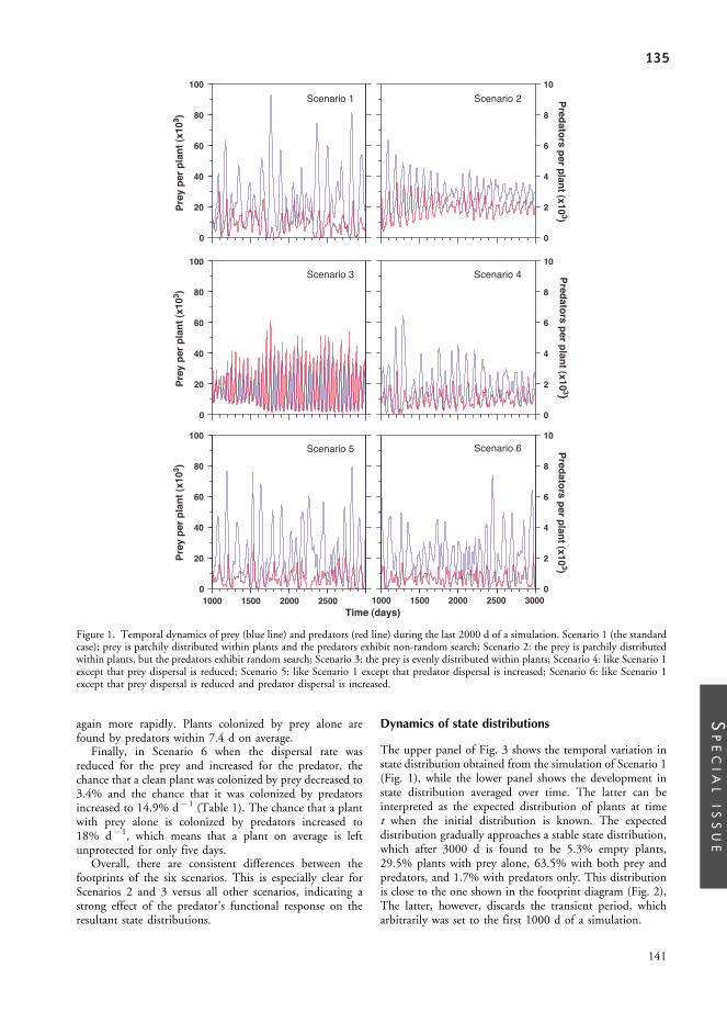
135
connecting state j with state i. By discarding the first 1000 dof a simulation we achieved convergence of the averagevalues of qi (t) and aij (t) to values that are insensitive toshort-term variations and thus reflect properties (or ‘‘foot-prints’’) of the underlying processes.
Modeling transition probabilities
If tests for time-homogeneity show that transition prob-abilities vary with time, the next step is to investigatewhether the variation can be related to the current state ofthe system.
Since we had no a priori assumptions concerning thequantitative relationships between transition probabilitiesand state variables, we first formulated a fairly simple andgeneral model for such a relationship, namely
aij� cijLij (q)bij (05aij51; 05 cij51) (3)
where Lij (q) is a linear combination of the four statevariables q1, q2, q3, and q4 (05Lij (q)51), while bij and cijare non-negative constants. Thus, bij�0 implies that aij isindependent of the current state of the system and equal tocij, whereas bij�0 means that aij increases with Lij (q)provided cij�0. The relationship between Lij (q) and aij isdownward accelerating for 0BbijB1, linear for bij�1 andupward accelerating for bij�1.
For each of the 12 non-zero matrix elements (aij) wescreened all 14 linear combinations of q1, q2, q3, and q4(except the sum of all four) to find the linear combinationthat yielded the highest positive Spearman correlationcoefficient between aij and Lij (q). This linear combinationwas then chosen as candidate for estimating the parametersof eq. 3. The Solver tool in Excel was used to maximize thelog likelihood function (Supplementary material) by meansof iteration. Once the best set of parameter values had beenidentified, we used Akaike’s information criterion (AIC ) totest whether a state-dependent model performed signifi-cantly better than the concomitant state-independent modelderived by setting bij�0. The difference between themodels was tested by means of a x2-test, because twicethe difference in AIC between the full and the reducedmodel, nested within the former, is distributed approxi-mately as x2 with n degrees of freedom, where n is thedifference in DF between the two models (Hilborn andMangel 1997).
Matrix modeling
When the transition probabilities of the projection matrix(eq. 1) have been parameterized based on eq. 3, the modelcan be reiterated to reveal the system’s dynamics. Inparticular we are interested in finding the long-term(asymptotic) steady state distribution of Q or q, becausethis tells us whether the system is inherently stable withrespect to coexistence of prey and predators, i.e. the systemreturns to equilibrium after a small perturbation. Since thesystem may possess more than a single steady state, thestability domain was explored by varying the initial statedistribution (denoted Q(0) or q(0)).
We examined the effect of the initial state distributionon the asymptotic behavior of the model by varying q1(0),q2(0), q3(0), and q4(0) in steps of 0.1 under the constraintthat the four state variables should sum to unity. This gives286 different combinations.
Results
The simulations and their footprints
Figure 1 shows the predator-prey fluctuations of the sixscenarios while Fig. 2 shows the concomitant footprints.Table 1 summarizes the outcome of all simulationsincluding the replicated runs of Scenario 1.
In Scenario 1 both species exhibited violent and irregularfluctuations. As seen from Fig. 2, on average, 95.9% of theplants were occupied by mites. 67.1% of the plants hostedboth species, 27.1% only prey and 1.6% only predators.Clean plants had on average 4.9% chance per day of beingcolonized by prey and 4.1% chance of being colonized bypredators. Once a plant was inhabited by prey, its chance ofalso being colonized by predators was 7.2% per day, whichmeans that the average time elapsing from being invaded byprey to being colonized by predators can be found as
1
�ln(1� 0:072)�13.4 d.
In Scenarios 2 and 3, the predators were assumed toforage less efficiently than in Scenario 1. As a consequencethey were unable to eradicate the prey from a plant, soplants in state 4 were absent and the same applies to plantsin State 1. Occasionally predators went extinct on a plantbut the likelihood of such an event was 0.3 and 1.1% d�1
for Scenarios 2 and 3, respectively. Plants with only preywere almost immediately colonized by predators, so thatplants on average remained unprotected for only two days.Thus, the lower efficiency of the predators was compensatedby their ubiquitous presence. Both scenarios were signifi-cantly different from Scenario 1 with respect to statevariables and transition probabilities (log-linear analysis:pB0.001); accordingly, the footprints (Fig. 2b, c) look verydifferent.
The reduced dispersal rate of the prey in Scenario 4caused a significant reduction in the percentage of plantswith prey only (from 27.1% in Scenario 1 to 14.8% inScenario 4), partly because the transition probability fromclean to prey infested plants declined from 4.9% inScenario 1 to 3.9% in Scenario 4, and partly becauseplants with prey alone were more quickly infested withpredators in the latter scenario. The proportions of plantswith both species and with predators alone weresignificantly higher in Scenario 4 than in Scenario 1(Table 1).
The increased dispersal rate of the predators in Scenario5 significantly increased the transition probability fromState 1 to State 4 and vice versa, and from State 2 to State 3and vice versa in comparison with Scenario 1 (Table 1).This shows that the highly mobile predators more quicklycolonize new plants but on the other hand also leave them
140
SPEC
IA
LISSU
E again more rapidly. Plants colonized by prey alone arefound by predators within 7.4 d on average.
Finally, in Scenario 6 when the dispersal rate wasreduced for the prey and increased for the predator, thechance that a clean plant was colonized by prey decreased to3.4% and the chance that it was colonized by predatorsincreased to 14.9% d�1 (Table 1). The chance that a plantwith prey alone is colonized by predators increased to18% d�1, which means that a plant on average is leftunprotected for only five days.
Overall, there are consistent differences between thefootprints of the six scenarios. This is especially clear forScenarios 2 and 3 versus all other scenarios, indicating astrong effect of the predator’s functional response on theresultant state distributions.
Dynamics of state distributions
The upper panel of Fig. 3 shows the temporal variation instate distribution obtained from the simulation of Scenario 1(Fig. 1), while the lower panel shows the development instate distribution averaged over time. The latter can beinterpreted as the expected distribution of plants at timet when the initial distribution is known. The expecteddistribution gradually approaches a stable state distribution,which after 3000 d is found to be 5.3% empty plants,29.5% plants with prey alone, 63.5% with both prey andpredators, and 1.7% with predators only. This distributionis close to the one shown in the footprint diagram (Fig. 2),The latter, however, discards the transient period, whicharbitrarily was set to the first 1000 d of a simulation.
0
20
40
60
80
100
Pre
y p
er p
lan
t (x
103 )
Scenario 1
0
2
4
6
8
10
Pred
ators p
er plan
t (x103)
Scenario 2
0
20
40
60
80
100
Pre
y p
er p
lan
t (x
103 )
Scenario 3
0
2
4
6
8
10
Pred
ators p
er plan
t (x103)
Scenario 4
1000 1500 2000 25000
20
40
60
80
100
Pre
y p
er p
lan
t (x
103 )
Scenario 5
1000 1500 2000 2500 30000
2
4
6
8
10
Pred
ators p
er plan
t (x103)
Scenario 6
Time (days)
Figure 1. Temporal dynamics of prey (blue line) and predators (red line) during the last 2000 d of a simulation. Scenario 1 (the standardcase); prey is patchily distributed within plants and the predators exhibit non-random search; Scenario 2: the prey is patchily distributedwithin plants, but the predators exhibit random search; Scenario 3: the prey is evenly distributed within plants; Scenario 4: like Scenario 1except that prey dispersal is reduced; Scenario 5: like Scenario 1 except that predator dispersal is increased; Scenario 6: like Scenario 1except that prey dispersal is reduced and predator dispersal is increased.
141
SPEC
IA
LISSU
E

136
Variation among scenarios
The six replicates of Scenario 1 showed little variationamong the individual replicates. Thus, the coefficient ofvariation (CV) ranged from 0.05 to 1.2% for the statevariables, and from 0.002 to 1.9% for the transitionprobabilities. The variation among scenarios was consider-ably larger than the within-scenario variation, both withrespect to state variables and transition probabilities (Table 1)which is a prerequisite for comparing footprints obtainedfrom scenarios with different population dynamics. Thus,Scenario 1 could be separated from the five other scenarioson at least one, but in most cases several, parameters.
Test for stationarity
The log-linear analyses of the transition matrices clearlyshowed for all scenarios that the transition probabilitieswere non-stationary (pB0.0001). Consequently, at leastsome of the transition probabilities are likely to be state-dependent.
Modeling transition probabilities
Table 2 gives an overview of those linear combinations of qi(i�1, 2, 3, 4) that correlated best with the transitions
20.7%
14.9%
81.0%
0.3%
3.4%
81.6%
18.0%
4.0%95.7%
3.0%
0.3%
75.4%
4.5%
17.1%
3.8%
74.6%
17.7%
4.1%
90.7%
0.2%
4.9%
92.5%
7.2%
2.7%
97.0%
2.4%
0.3%
79.1%
27.1%
1.6%
4.1%
67.1%
59.9%
40.1%
0.3%
99.7%
0.6%
99.4%
98.9%1.1%
40.3%
59.7%
2.8%
97.2%13.6%
7.9%
87.6%
0.3%
3.9%
86.6%
13.1%
2.3%
97.3%
2.6%
0.3%
83.2%
4.6%
3.7%
77.0%
14.8%
25.8%
8.9%
86.2%
0.3%
4.3%
87.1%
12.6%
4.5%95.2%
3.1%
0.2%
70.0%
25.2%
4.3%
68.7%
1.9%
Scenario 1 Scenario 2
Scenario 3 Scenario 4
Scenario 5 Scenario 6
Figure 2. Transition diagrams (also called ‘‘footprints’’) of the six scenarios. The framed values show the proportion of total time plantson average spend in the various states (also indicated by the circle’s area). The arrows connecting the states mark the transitions with theassociated transition probabilities annotated. Note that the transition probabilities from a state may not necessarily sum to unity becauserare transitions involving more than a single event are omitted. State 1 (green) is empty, State 2 (blue) is with prey alone, State 3 (purple)is with both species and State 4 (red) is with predators alone.
142
SPEC
IA
LISSU
E
obtained from Scenario 1. All relationships are highlysignificant and confirm the a priori assumption thatcolonization probabilities of plants without prey (a21 anda34) correlate with the proportion of plants alreadyoccupied by prey (q2�q3) and that the probabilities ofplants without predators being colonized by predators (a41and a32) correlate best with the proportion of plants alreadyoccupied by predators (q3�q4). The probabilities that preygoes extinct depend on whether predators are present on theplant. In the absence of predators, the extinction probability(a12) declines with an increase in q2, whereas a43 declineswith an increase in q3 in the presence of predators.Similarly, the probabilities that predators go extinct dependon whether prey is present. When prey is present, a23decreases as q3 increases; when there is no prey a14 decreasesas q4 increases.
The remaining transitions occurred with low frequenciesand the probabilities of these transitions were all set to 0.Hence, the eight transition probabilities listed in Table 2require estimation of 16 parameters.
Table 3 summarizes the results of the maximumlikelihood analyses. All analyses except for a14 yieldedpositive values of both bij and cij (eq. 3), though b34 was notsignificantly different from 0 and was therefore replaced by 0.In the remaining six cases, setting bij equal to 0 resulted in asignificant increase in AIC, which confirms that thesetransitions are indeed state-dependent.
The model for a21 indicates that empty plants will becolonized by prey with an increasing probability as theproportion of plants occupied by prey increases and willapproach a maximum of ca 9% d�1. Likewise, theprobability that an empty plant becomes occupiedby predators increases with the proportion of plantsalready occupied by predators up to a maximum of ca13% d�1.
The models for a12 and a32 show that transitionsfrom plants inhabited by prey to empty plants occurwith decreasing probability the higher the proportionof prey plants is, while the probability of transitionsfrom plants with only prey to plants with bothspecies increases with the proportion of plants alreadyoccupied by predators. The former transition is a muchslower process than the latter, which has a maximum of�16% d�1.
The models for a23 and a43 show that the transitionprobabilities accelerate as the proportion of plantsoccupied by both prey and predators approaches 0.However, the maximum probabilities for both processesare low, especially for the rate at which plants becomedevoid of prey (a43), indicating that once a plant isinhabited by both species it takes rather long time beforethe predators have eradicated the prey, partly due to thefact that both prey and predators continuously immigrateto such plants.
Finally, the models for a34 and a14 show that these twoprobabilities can be regarded as state-independent. Theparameters indicate that predators quickly disappearfrom plants without prey (a14�0.19), whereas plantsoccupied by only predators are rather unlikely to be(re)colonized by prey (a34�0.0058).Ta
ble
1.ComparisonsbetweenScen
ario
1an
dthefive
other
scen
arios.Values
inbold
falloutsidethe95%
confiden
celimitsforScen
ario
1obtained
from
sixreplicatedruns.q1�per
centofplantsin
State1(neither
preynorpredators),q2�per
centofplantsin
State2(only
prey),q3�per
centofplantsin
State3(both
preyan
dpredators),q4�per
centofplantsin
State4(only
predators).a ijisthe
estimated
probab
ilitythat
aplantin
statejat
day
twillbein
statei(i,j�
1,2,3,4)at
day
t�1.
Scen
ario
States
(%)
Tran
sitionprobab
ilities(%
)
q1
q2
q3
q4
a 11
a 21
a 31
a 41
a 12
a 22
a 32
a 42
a 13
a 23
a 33
a 43
a 14
a 24
a 34
a 44
Scen
ario
1(avg)
4.05
27.09
67.12
1.63
90.72
4.87
0.27
4.10
0.25
92.52
7.20
0.02
0.02
2.70
97.02
0.26
17.73
0.73
2.43
79.08
lower
limit
2.07
21.80
59.70
1.29
87.69
3.81
0.11
2.46
0.15
90.70
5.46
0.01
0.01
2.43
96.71
0.18
15.71
0.40
1.60
77.33
upper
limit
6.69
32.96
74.97
2.00
93.80
6.06
0.49
6.15
0.36
94.36
9.17
0.03
0.04
2.97
97.34
0.35
19.89
1.16
3.43
80.84
Scen
ario
20.00
0.65
99.35
0.00
0.00
0.00
0.00
100.00
0.00
59.87
40.13
0.00
0.00
0.26
99.74
0.00
8.33
0.00
25.00
66.67
Scen
ario
30.00
2.76
97.24
0.00
0.00
0.00
0.00
0.00
0.00
59.70
40.30
0.00
0.00
1.15
98.85
0.00
0.00
0.00
16.67
83.33
Scen
ario
44.55
14.76
76.99
3.70
87.65
3.92
0.58
7.85
0.29
86.59
13.08
0.03
0.02
2.31
97.34
0.33
13.62
0.51
2.63
83.24
Scen
ario
54.30
25.15
68.66
1.89
86.23
4.32
0.52
8.94
0.31
87.05
12.59
0.05
0.04
4.48
95.23
0.25
25.76
1.21
3.05
69.98
Scen
ario
64.51
17.08
74.65
3.77
80.97
3.37
0.81
14.86
0.34
81.57
18.00
0.08
0.04
3.97
95.67
0.33
20.68
0.88
3.01
75.43
143
SPEC
IA
LISSU
E

137
Variation among scenarios
The six replicates of Scenario 1 showed little variationamong the individual replicates. Thus, the coefficient ofvariation (CV) ranged from 0.05 to 1.2% for the statevariables, and from 0.002 to 1.9% for the transitionprobabilities. The variation among scenarios was consider-ably larger than the within-scenario variation, both withrespect to state variables and transition probabilities (Table 1)which is a prerequisite for comparing footprints obtainedfrom scenarios with different population dynamics. Thus,Scenario 1 could be separated from the five other scenarioson at least one, but in most cases several, parameters.
Test for stationarity
The log-linear analyses of the transition matrices clearlyshowed for all scenarios that the transition probabilitieswere non-stationary (pB0.0001). Consequently, at leastsome of the transition probabilities are likely to be state-dependent.
Modeling transition probabilities
Table 2 gives an overview of those linear combinations of qi(i�1, 2, 3, 4) that correlated best with the transitions
20.7%
14.9%
81.0%
0.3%
3.4%
81.6%
18.0%
4.0%95.7%
3.0%
0.3%
75.4%
4.5%
17.1%
3.8%
74.6%
17.7%
4.1%
90.7%
0.2%
4.9%
92.5%
7.2%
2.7%
97.0%
2.4%
0.3%
79.1%
27.1%
1.6%
4.1%
67.1%
59.9%
40.1%
0.3%
99.7%
0.6%
99.4%
98.9%1.1%
40.3%
59.7%
2.8%
97.2%13.6%
7.9%
87.6%
0.3%
3.9%
86.6%
13.1%
2.3%
97.3%
2.6%
0.3%
83.2%
4.6%
3.7%
77.0%
14.8%
25.8%
8.9%
86.2%
0.3%
4.3%
87.1%
12.6%
4.5%95.2%
3.1%
0.2%
70.0%
25.2%
4.3%
68.7%
1.9%
Scenario 1 Scenario 2
Scenario 3 Scenario 4
Scenario 5 Scenario 6
Figure 2. Transition diagrams (also called ‘‘footprints’’) of the six scenarios. The framed values show the proportion of total time plantson average spend in the various states (also indicated by the circle’s area). The arrows connecting the states mark the transitions with theassociated transition probabilities annotated. Note that the transition probabilities from a state may not necessarily sum to unity becauserare transitions involving more than a single event are omitted. State 1 (green) is empty, State 2 (blue) is with prey alone, State 3 (purple)is with both species and State 4 (red) is with predators alone.
142
SPEC
IA
LISSU
E
obtained from Scenario 1. All relationships are highlysignificant and confirm the a priori assumption thatcolonization probabilities of plants without prey (a21 anda34) correlate with the proportion of plants alreadyoccupied by prey (q2�q3) and that the probabilities ofplants without predators being colonized by predators (a41and a32) correlate best with the proportion of plants alreadyoccupied by predators (q3�q4). The probabilities that preygoes extinct depend on whether predators are present on theplant. In the absence of predators, the extinction probability(a12) declines with an increase in q2, whereas a43 declineswith an increase in q3 in the presence of predators.Similarly, the probabilities that predators go extinct dependon whether prey is present. When prey is present, a23decreases as q3 increases; when there is no prey a14 decreasesas q4 increases.
The remaining transitions occurred with low frequenciesand the probabilities of these transitions were all set to 0.Hence, the eight transition probabilities listed in Table 2require estimation of 16 parameters.
Table 3 summarizes the results of the maximumlikelihood analyses. All analyses except for a14 yieldedpositive values of both bij and cij (eq. 3), though b34 was notsignificantly different from 0 and was therefore replaced by 0.In the remaining six cases, setting bij equal to 0 resulted in asignificant increase in AIC, which confirms that thesetransitions are indeed state-dependent.
The model for a21 indicates that empty plants will becolonized by prey with an increasing probability as theproportion of plants occupied by prey increases and willapproach a maximum of ca 9% d�1. Likewise, theprobability that an empty plant becomes occupiedby predators increases with the proportion of plantsalready occupied by predators up to a maximum of ca13% d�1.
The models for a12 and a32 show that transitionsfrom plants inhabited by prey to empty plants occurwith decreasing probability the higher the proportionof prey plants is, while the probability of transitionsfrom plants with only prey to plants with bothspecies increases with the proportion of plants alreadyoccupied by predators. The former transition is a muchslower process than the latter, which has a maximum of�16% d�1.
The models for a23 and a43 show that the transitionprobabilities accelerate as the proportion of plantsoccupied by both prey and predators approaches 0.However, the maximum probabilities for both processesare low, especially for the rate at which plants becomedevoid of prey (a43), indicating that once a plant isinhabited by both species it takes rather long time beforethe predators have eradicated the prey, partly due to thefact that both prey and predators continuously immigrateto such plants.
Finally, the models for a34 and a14 show that these twoprobabilities can be regarded as state-independent. Theparameters indicate that predators quickly disappearfrom plants without prey (a14�0.19), whereas plantsoccupied by only predators are rather unlikely to be(re)colonized by prey (a34�0.0058).Ta
ble
1.ComparisonsbetweenScen
ario
1an
dthefive
other
scen
arios.Values
inbold
falloutsidethe95%
confiden
celimitsforScen
ario
1obtained
from
sixreplicatedruns.q1�per
centofplantsin
State1(neither
preynorpredators),q2�per
centofplantsin
State2(only
prey),q3�per
centofplantsin
State3(both
preyan
dpredators),q4�per
centofplantsin
State4(only
predators).a ijisthe
estimated
probab
ilitythat
aplantin
statejat
day
twillbein
statei(i,j�
1,2,3,4)at
day
t�1.
Scen
ario
States
(%)
Tran
sitionprobab
ilities(%
)
q1
q2
q3
q4
a 11
a 21
a 31
a 41
a 12
a 22
a 32
a 42
a 13
a 23
a 33
a 43
a 14
a 24
a 34
a 44
Scen
ario
1(avg)
4.05
27.09
67.12
1.63
90.72
4.87
0.27
4.10
0.25
92.52
7.20
0.02
0.02
2.70
97.02
0.26
17.73
0.73
2.43
79.08
lower
limit
2.07
21.80
59.70
1.29
87.69
3.81
0.11
2.46
0.15
90.70
5.46
0.01
0.01
2.43
96.71
0.18
15.71
0.40
1.60
77.33
upper
limit
6.69
32.96
74.97
2.00
93.80
6.06
0.49
6.15
0.36
94.36
9.17
0.03
0.04
2.97
97.34
0.35
19.89
1.16
3.43
80.84
Scen
ario
20.00
0.65
99.35
0.00
0.00
0.00
0.00
100.00
0.00
59.87
40.13
0.00
0.00
0.26
99.74
0.00
8.33
0.00
25.00
66.67
Scen
ario
30.00
2.76
97.24
0.00
0.00
0.00
0.00
0.00
0.00
59.70
40.30
0.00
0.00
1.15
98.85
0.00
0.00
0.00
16.67
83.33
Scen
ario
44.55
14.76
76.99
3.70
87.65
3.92
0.58
7.85
0.29
86.59
13.08
0.03
0.02
2.31
97.34
0.33
13.62
0.51
2.63
83.24
Scen
ario
54.30
25.15
68.66
1.89
86.23
4.32
0.52
8.94
0.31
87.05
12.59
0.05
0.04
4.48
95.23
0.25
25.76
1.21
3.05
69.98
Scen
ario
64.51
17.08
74.65
3.77
80.97
3.37
0.81
14.86
0.34
81.57
18.00
0.08
0.04
3.97
95.67
0.33
20.68
0.88
3.01
75.43
143
SPEC
IA
LISSU
E

138
Matrix modeling
The exploration of the asymptotic behavior of the matrixmodel parameterized by means of data from Scenario 1revealed that the long-term state distribution (denotedq�i )depends on the initial conditions. Hence, the model is non-ergodic (Caswell 2001). Three of the asymptotic statedistributions are identical to the initial state distributionsand occur when the systems starts in a completelysynchronized state, i.e. q�1�q1(0) �1 (all plants are clean),q�2�q2(0) �1 (all plants are occupied by prey) or q�3�q3(0) �1 (all plants are occupied by both prey andpredators). The fourth synchronized state with all plantsoccupied by predators alone (i.e. q�
4�q4(0)�1) of coursequickly leads to an equilibrium where all plants areclean (i.e. q�
1 �1): However, if the initial distribution is
asynchronous, i.e. qi(0)B1 for all i, the system willconverge toward one of three asymptotic states (Fig. 4): a)extinction of both species, b) extinction of predators and avery high (99.95%) frequency of prey-infested plants, andc) coexistence of both species with 4.46% of the plants inState 1, 21.67% in State 2, 71.26% in State 3, and 2.61%in State 4. Outcome (a) occurred in 44% of the cases andwas associated with combinations where the initial propor-tion of plants with prey was low relative to the proportionof plants with predators. Outcome (b) occurred in 35% ofthe cases and was associated with combinations where theinitial proportion of plants with prey was high and theproportion with predators low. Finally, outcome (c)occurred in 21% of the cases and was associated withcombinations where the initial proportions of plants withprey (q2(0)�q3(0)) and with predators (q3(0)�q4(0)) wereboth high. In particular, all cases where 0.645q3(0)B1lead to outcome (c) irrespective of the three other states.Outcome (c) agrees well with that obtained from thesimulation model (Fig. 3 lower panel), although 3000 d ofsimulation is not sufficient for the system to attain a steady-state distribution.
Discussion
Our preliminary study, based on a single specific model anda few characteristic scenarios, has demonstrated thatcomplex population dynamics can be summarized by meansof simple state transition diagrams which are likely torepresent ‘‘footprints’’ of the underlying population pro-cesses. Thus, the footprints of predator�prey dynamics arecomposed by merely four state variables, each representingpresence/absence of prey and predators, as well as theconnections between these states. Connectivity is expressedin terms of transition probabilities which provide informa-tion about the turn-over rates of the states. This may serveas a diagnostic tool in biological control programmes,because the time elapsing from a plant becomes infestedwith a pest organism to it is found by a natural enemy isoften crucial (Huffaker and Messenger 1964). Likewise,turn-over rates can be used to forecast the risk of localextinctions, a factor that may influence the persistence ofspecies living in fragmented habitats (Burkey 1989). In fact,many metapopulation (Hanski 1999) and biogeographicalstudies (Soberon 2010) rely on incidence data only, and insuch cases it can be valuable if a link from this type of data
0
0.1
0.2
0.3
0.4
0.5
0.6
0.7
0.8
0.9
1
1000 1500 2000 2500 3000Days
Pro
po
rtio
n o
f p
lan
ts
0
0.1
0.2
0.3
0.4
0.5
0.6
0.7
0.8
0.9
1
1000 1500 2000 2500 3000Days
Pro
po
rtio
n o
f p
lan
ts
Figure 3. Upper panel: temporal variation in the distribution ofplants based on Scenario 1. Lower panel: expected state distribu-tion at time t obtained by cumulating the distributions in theupper panel and then averaging over time. Colours as in Fig. 2.
Table 2. List of functions yielding the highest positive Spearman correlation coefficient between state variables (qi) and transitionprobabilities (aij) obtained from Scenario 1. The functions tested comprise all linear combinations of qi (i.e. q1, q2, q3, q4, q1�q2, q1�q3,q1�q4, q2�q3, q2�q4, q3�q4, 1�q1, 1�q2, 1�q3, and 1�q4) except q1�q2�q3�q4�1.
Transition probability (aij) Function (Lij(q)) Corr. coeff. (rs) Sample size (n) p
a21 c21(q2�q3)b21 0.809 964 B0.0001
a41 c41(q3�q4)b41 0.627 824 B0.0001
a12 c12(1�q2)b12 0.716 448 B0.0001
a32 c32(q3�q4)b32 0.775 1979 B0.0001
a23 c23(1�q3)b23 0.474 1869 B0.0001
a43 c43(1�q3)b43 0.546 817 B0.0001
a34 c34(q2�q3)b34 0.475 255 B0.0001
a14 c14(1�q4)b14 0.462 1040 B0.0001
144
SPEC
IA
LISSU
E
and back to the underlying population dynamics can beestablished via the footprints.
In this study we used plants as the units of measurement.However, the footprints obtained from Scenarios 2 and 3(Fig. 2) indicate that this spatial unit may not be optimalbecause State 3 dominates at the expense of especially State1 and 4. Thus, using a smaller spatial scale (e.g. a leaf as inNachman 1999) will increase the proportion of the emptypatches and patches occupied by only a single species.Applying a smaller scale would also make sampling easierand increase the creditability of absences (Soberon 2010).On the other hand, if sampling units become very small,occupied patches will become too rare. It is thereforeimportant to choose an appropriate spatial unit formeasuring and interpreting spatial dynamics (Wiens 1989,Rahbek 2005).
The transition matrices were found to be non-stationary,confirming our expectation that at least some of thetransition probabilities vary with time. As Gurney andNisbet (1978), we assumed that the temporal variations intransition probabilities are due to feed-backs between statevariables and transition probabilities, although the relation-ships linking them are not necessarily linear (as assumed byGurney and Nisbet 1978). By fitting a generic model to thetransition probabilities obtained from Scenario 1 we wereable to describe this non-stationarity: the results demon-strate a strong positive feed-back between the chance that anempty plant becomes colonized by prey and the proportionof plants already occupied by prey. Likewise, plants withoutpredators will quickly become occupied by predators whenthis species already inhabits the majority of plants.
Extinction probabilities, on the other hand, were notalways state-dependent. In the cases where extinctionprobabilities were found to be state-dependent, the func-tional relationships show that extinction probability in-creases as the number of extant populations declines. Thiscreates positive feedbacks which tend to accelerate existingtrends and make the system sensitive to perturbations thateventually lead to extinction. The stability analysis revealedthat the projection model based on Scenario 1 is non-ergodic, i.e. its asymptotic state distribution depends on itsinitial state (Caswell 2001). Six different equilibria wereidentified: a) all plants are clean, b) all plants are inhabitedby prey, c) all plants are occupied by both prey andpredators, d) 99.95% plants are occupied by prey while theremaining are clean, and e) 4.46% of the plants are clean,21.67% infested with prey alone, 71.26% with both prey
Table 3. Maximum likelihood estimates of the parameters used to model the state-dependent transition probabilities in Table 2 obtained fromScenario 1. bij is either estimated to be 0 (as for a14) or to be so close to 0 (as for a34) that it can be set to 0 (i.e. the transition probability isstate-independent). p is the probability that a state-dependent and a state-independent model are equally good to fit data. State-dependentprobabilities are only used if pB0.05.
Transition probability (aij) bij cij DAIC x21 p
a21 4.542 0.088 242.2 483.7 B0.0001a41 2.378 0.134 445.2 967.4 B0.0001a12 0.596 0.0041 18.4 36.8 B0.0001a32 1.477 0.163 2818.3 5636.5 B0.0001a23 0.627 0.063 1288.8 2577.6 B0.0001a43 0.209 0.0040 19.2 38.3 B0.0001a34 0 0.0058 0.027 0.053 0.82a14 0 0.190 0 0 1
0
0.1
0.2
0.3
0.4
0.5
0.6
0.7
0.8
0.9
1
0 100 200 300 400 500 600 700 800 900 1000Days
Cu
mu
late
d p
rop
ort
ion
of
pla
nts
00.10.20.30.40.50.60.70.80.9
1
0 100 200 300 400 500 600 700 800 900 1000Days
Cu
mu
late
d p
rop
ort
ion
of
pla
nts
00.10.20.30.40.50.60.70.80.9
1
0 100 200 300 400 500 600 700 800 900 1000Days
Cu
mu
late
d p
rop
ort
ion
of
pla
nts
Figure 4. Predictions for Scenario 1 based on the matrix model(eq. 1) and with parameter values given in Table 3 for threedifferent initial state distributions. Upper panel: 40% in State 1,10% in State 2, 30% in State 3, and 20% in State 4. Middle panel:40% in State 1, 30% in State 2, 20% in State 3, and 10% in State4. Lower panel: 20% in State 1, 40% in State 2, 30% in State 3,and 10% in State 4. Colours as in Fig. 2.
145
SPEC
IA
LISSU
E
139
Matrix modeling
The exploration of the asymptotic behavior of the matrixmodel parameterized by means of data from Scenario 1revealed that the long-term state distribution (denotedq�i )depends on the initial conditions. Hence, the model is non-ergodic (Caswell 2001). Three of the asymptotic statedistributions are identical to the initial state distributionsand occur when the systems starts in a completelysynchronized state, i.e. q�1�q1(0) �1 (all plants are clean),q�2�q2(0) �1 (all plants are occupied by prey) or q�3�q3(0) �1 (all plants are occupied by both prey andpredators). The fourth synchronized state with all plantsoccupied by predators alone (i.e. q�
4�q4(0)�1) of coursequickly leads to an equilibrium where all plants areclean (i.e. q�
1 �1): However, if the initial distribution is
asynchronous, i.e. qi(0)B1 for all i, the system willconverge toward one of three asymptotic states (Fig. 4): a)extinction of both species, b) extinction of predators and avery high (99.95%) frequency of prey-infested plants, andc) coexistence of both species with 4.46% of the plants inState 1, 21.67% in State 2, 71.26% in State 3, and 2.61%in State 4. Outcome (a) occurred in 44% of the cases andwas associated with combinations where the initial propor-tion of plants with prey was low relative to the proportionof plants with predators. Outcome (b) occurred in 35% ofthe cases and was associated with combinations where theinitial proportion of plants with prey was high and theproportion with predators low. Finally, outcome (c)occurred in 21% of the cases and was associated withcombinations where the initial proportions of plants withprey (q2(0)�q3(0)) and with predators (q3(0)�q4(0)) wereboth high. In particular, all cases where 0.645q3(0)B1lead to outcome (c) irrespective of the three other states.Outcome (c) agrees well with that obtained from thesimulation model (Fig. 3 lower panel), although 3000 d ofsimulation is not sufficient for the system to attain a steady-state distribution.
Discussion
Our preliminary study, based on a single specific model anda few characteristic scenarios, has demonstrated thatcomplex population dynamics can be summarized by meansof simple state transition diagrams which are likely torepresent ‘‘footprints’’ of the underlying population pro-cesses. Thus, the footprints of predator�prey dynamics arecomposed by merely four state variables, each representingpresence/absence of prey and predators, as well as theconnections between these states. Connectivity is expressedin terms of transition probabilities which provide informa-tion about the turn-over rates of the states. This may serveas a diagnostic tool in biological control programmes,because the time elapsing from a plant becomes infestedwith a pest organism to it is found by a natural enemy isoften crucial (Huffaker and Messenger 1964). Likewise,turn-over rates can be used to forecast the risk of localextinctions, a factor that may influence the persistence ofspecies living in fragmented habitats (Burkey 1989). In fact,many metapopulation (Hanski 1999) and biogeographicalstudies (Soberon 2010) rely on incidence data only, and insuch cases it can be valuable if a link from this type of data
0
0.1
0.2
0.3
0.4
0.5
0.6
0.7
0.8
0.9
1
1000 1500 2000 2500 3000Days
Pro
po
rtio
n o
f p
lan
ts
0
0.1
0.2
0.3
0.4
0.5
0.6
0.7
0.8
0.9
1
1000 1500 2000 2500 3000Days
Pro
po
rtio
n o
f p
lan
ts
Figure 3. Upper panel: temporal variation in the distribution ofplants based on Scenario 1. Lower panel: expected state distribu-tion at time t obtained by cumulating the distributions in theupper panel and then averaging over time. Colours as in Fig. 2.
Table 2. List of functions yielding the highest positive Spearman correlation coefficient between state variables (qi) and transitionprobabilities (aij) obtained from Scenario 1. The functions tested comprise all linear combinations of qi (i.e. q1, q2, q3, q4, q1�q2, q1�q3,q1�q4, q2�q3, q2�q4, q3�q4, 1�q1, 1�q2, 1�q3, and 1�q4) except q1�q2�q3�q4�1.
Transition probability (aij) Function (Lij(q)) Corr. coeff. (rs) Sample size (n) p
a21 c21(q2�q3)b21 0.809 964 B0.0001
a41 c41(q3�q4)b41 0.627 824 B0.0001
a12 c12(1�q2)b12 0.716 448 B0.0001
a32 c32(q3�q4)b32 0.775 1979 B0.0001
a23 c23(1�q3)b23 0.474 1869 B0.0001
a43 c43(1�q3)b43 0.546 817 B0.0001
a34 c34(q2�q3)b34 0.475 255 B0.0001
a14 c14(1�q4)b14 0.462 1040 B0.0001
144
SPEC
IA
LISSU
E
and back to the underlying population dynamics can beestablished via the footprints.
In this study we used plants as the units of measurement.However, the footprints obtained from Scenarios 2 and 3(Fig. 2) indicate that this spatial unit may not be optimalbecause State 3 dominates at the expense of especially State1 and 4. Thus, using a smaller spatial scale (e.g. a leaf as inNachman 1999) will increase the proportion of the emptypatches and patches occupied by only a single species.Applying a smaller scale would also make sampling easierand increase the creditability of absences (Soberon 2010).On the other hand, if sampling units become very small,occupied patches will become too rare. It is thereforeimportant to choose an appropriate spatial unit formeasuring and interpreting spatial dynamics (Wiens 1989,Rahbek 2005).
The transition matrices were found to be non-stationary,confirming our expectation that at least some of thetransition probabilities vary with time. As Gurney andNisbet (1978), we assumed that the temporal variations intransition probabilities are due to feed-backs between statevariables and transition probabilities, although the relation-ships linking them are not necessarily linear (as assumed byGurney and Nisbet 1978). By fitting a generic model to thetransition probabilities obtained from Scenario 1 we wereable to describe this non-stationarity: the results demon-strate a strong positive feed-back between the chance that anempty plant becomes colonized by prey and the proportionof plants already occupied by prey. Likewise, plants withoutpredators will quickly become occupied by predators whenthis species already inhabits the majority of plants.
Extinction probabilities, on the other hand, were notalways state-dependent. In the cases where extinctionprobabilities were found to be state-dependent, the func-tional relationships show that extinction probability in-creases as the number of extant populations declines. Thiscreates positive feedbacks which tend to accelerate existingtrends and make the system sensitive to perturbations thateventually lead to extinction. The stability analysis revealedthat the projection model based on Scenario 1 is non-ergodic, i.e. its asymptotic state distribution depends on itsinitial state (Caswell 2001). Six different equilibria wereidentified: a) all plants are clean, b) all plants are inhabitedby prey, c) all plants are occupied by both prey andpredators, d) 99.95% plants are occupied by prey while theremaining are clean, and e) 4.46% of the plants are clean,21.67% infested with prey alone, 71.26% with both prey
Table 3. Maximum likelihood estimates of the parameters used to model the state-dependent transition probabilities in Table 2 obtained fromScenario 1. bij is either estimated to be 0 (as for a14) or to be so close to 0 (as for a34) that it can be set to 0 (i.e. the transition probability isstate-independent). p is the probability that a state-dependent and a state-independent model are equally good to fit data. State-dependentprobabilities are only used if pB0.05.
Transition probability (aij) bij cij DAIC x21 p
a21 4.542 0.088 242.2 483.7 B0.0001a41 2.378 0.134 445.2 967.4 B0.0001a12 0.596 0.0041 18.4 36.8 B0.0001a32 1.477 0.163 2818.3 5636.5 B0.0001a23 0.627 0.063 1288.8 2577.6 B0.0001a43 0.209 0.0040 19.2 38.3 B0.0001a34 0 0.0058 0.027 0.053 0.82a14 0 0.190 0 0 1
0
0.1
0.2
0.3
0.4
0.5
0.6
0.7
0.8
0.9
1
0 100 200 300 400 500 600 700 800 900 1000Days
Cu
mu
late
d p
rop
ort
ion
of
pla
nts
00.10.20.30.40.50.60.70.80.9
1
0 100 200 300 400 500 600 700 800 900 1000Days
Cu
mu
late
d p
rop
ort
ion
of
pla
nts
00.10.20.30.40.50.60.70.80.9
1
0 100 200 300 400 500 600 700 800 900 1000Days
Cu
mu
late
d p
rop
ort
ion
of
pla
nts
Figure 4. Predictions for Scenario 1 based on the matrix model(eq. 1) and with parameter values given in Table 3 for threedifferent initial state distributions. Upper panel: 40% in State 1,10% in State 2, 30% in State 3, and 20% in State 4. Middle panel:40% in State 1, 30% in State 2, 20% in State 3, and 10% in State4. Lower panel: 20% in State 1, 40% in State 2, 30% in State 3,and 10% in State 4. Colours as in Fig. 2.
145
SPEC
IA
LISSU
E

140
and predators and 2.61% with predators alone. Case a istrivial, while case b and c represent unstable equilibriabecause infinitely small deviations from equilibrium willchange case b to case d and case c to case e. From abiological point of view case b and c represent artifacts,which can be attributed, at least partly, to the fact that themodel does not explicitly incorporate plant condition,which means that plants can host high densities of preywithout suffering permanent damage.
The advantages of using model-generated data toparameterize a discrete state model are: 1) it is a quickand easy way of obtaining lots of detailed data, 2) we knowexactly the processes that have produced these data, and 3)we do not need to worry about sampling error (cf. Gastonand McArdle 1994). Consequently, we can be quiteconfident that the estimated parameters are representativefor the studied system. However, the drawback of usingartificial data is that they can never be more correct than themodel that has generated them. Complex simulationmodels, irrespective of how realistic they are, or believedto be, will always represent unrealistic simplifications thatcan bias the results. Thus, by using simulated data toparameterize a Markov chain model, we risk to exaggerateerrors already present in the simulated data. It is thereforeimportant to validate model predictions against real dataoriginating from field studies before the model is used forpractical purposes.
It is possible to parameterize discrete state transitionmodels directly from field data (Woolhouse and Harmsen1989). However, field data are likely to be too coarse-grained unless sampling takes place with very short(e.g. daily) intervals, and to be influenced by factors thatcannot be controlled by the experimenter such as theweather. In contrast, a simulation model can be developedby means of data obtained from specific experimentsconducted under controlled conditions.
Clements and Harmsen (1991) used a mechanisticsimulation model to complement an empirical transitionmatrix model of an acarine predator�prey system andconcluded that the transition matrix produced accuratepredictions, but could not provide information on what willhappen if the system under study was subject to manipula-tion. In contrast, the mechanistic (or reductionist) simula-tion approach provided information on how complexbiological interactions affect population dynamics, butcould not be used as a predictive tool.
The projection matrix employed in this paper simulatesthe system deterministically, by regarding the transitionprobabilities as the expected rates of state transitions.However, if the system consists of a finite number ofpatches (plants) and especially if this number is small,stochastic phenomena may play an important role (Nisbetand Gurney 1982). Even if the environment is constant,endogenous stochastic processes like extinctions and colo-nizations will perturb the system and, depending on itscurrent state, be able to push it from one stability domain toanother. Such sudden shifts in predator�prey dynamics havebeen observed in experimental studies of spider mites andpredatory mites (van de Klashorst et al. 1992, Janssen et al.1997, McCauley et al. 2000) and do also occur when thesystem is modeled by means of a stochastic simulationmodel (Nachman 1987b).
The deterministic projection model can be made stochas-tic by using Monte Carlo methods to generate the actualnumber of transitions in a system consisting of N plantsbased on the multinomial distribution (Supplementarymaterial eq. S1). In a following paper we plan to pursuethis approach in order to develop a stochastic version of adiscrete state transition model that can be used as a tacticaltool to forecast short and long-term changes in the system.The reliability of the predictions will be evaluated on basis ofthe amount information available at day 0 (depends onsample size) and the length of the forecasted period. Finally,it should be noted that although the matrix model only needsinput data on a classification scale (i.e. presence/absence) andyields predictions on the same scale, proportions of samplingunits with prey and/or predators can easily be converted todensities using regression models based on e.g. the negativebinomial distribution (Wilson and Gerrard 1971) or theWeibull distribution (Nachman 1984).
References
Anderson, T. W. and Goodman, L. A. 1957. Statistical inferenceabout Markov chains. � Ann. Math. Stat. 28: 89�110.
Burkey, T. V. 1989. Extinction in nature reserves: the effect offragmentation and the importance of migration betweenreserve fragments. � Oikos 55: 75�81.
Caswell, H. 2001. Matrix population models. � Sinauer.Clements, D. R. and Harmsen, R. 1991. A mechanistic simulation
to complement an empirical transition matrix model of acarinepopulation dynamics. � Ecol. Model. 59: 257�277.
Dharmadhikari, S. W. 1963. Functions of finite Markov chains.� Ann. Math. Stat. 34: 1022�1032.
Gaston, K. J. and McArdle, B. H. 1994. The temporal variabilityof animal abundance: measures, methods and patterns. � Phil.Trans. R. Soc. B 345: 335�358.
Gurney, W. S. C and Nisbet, R. M. 1978. Predator�preyfluctuations in patchy environments. � J. Anim. Ecol. 47:85�102.
Gurney, W. S. C. et al. 1998. Circles and spirals: populationpersistence in a spatially explicit predator�prey model.� Ecology 79: 2516�2539.
Hanski., I. 1999. Metapopulation ecology. � Oxford Univ. Press.Helle, W. and Sabelis, M. W. 1985. Spider mites. Their biology,
natural enemies and control. � Elsevier.Hilborn, R. and Mangel, M. 1997. The ecological detective.
� Princeton Univ. Press.Holling, C. S. 1959. Some characteristics of simple types of
predation and parasitism. � Can. Entomol. 91: 385�398.Huffaker, C. B. 1958. Experimental studies of predation: dispersal
factors and predator�prey oscillations. � Hilgardia 27: 343�383.
Huffaker, C. B. and Messenger, P. S. 1964. The concept andsignificance of natural control. � In: DeBach, P. (ed.),Biological control of insect pests & weeds. Chapman andHall, pp. 74�117.
Huffaker, C. B. et al. 1963. Experimental studies on predation:complex dispersion and levels of food in acarine predator�preyinteraction. � Hilgardia 34: 305�330.
Janssen, A. et al. 1997. Metapopulation dynamics of a persistingpredator�prey system in the laboratory: time-series analysis.� Exp. Appl. Acarol. 21: 415�430.
Levins, R. 1969. Some demographic and genetic consequences ofenvironmental heterogeneity for biological control. � Bull.Entomol. Soc. Am. 15: 237�240.
146
SPEC
IA
LISSU
E
Lotka, A. J. 1925. Elements of physical biology. � Williams andWilkins. Reprinted in 1956. Elements of mathematicalbiology. Dover Publ.
Lusseau, D. 2003. Effects of tour boats on the behaviour ofbottlenose dolphins: using Markov Chains to model anthro-pogenic impacts. � Conserv. Biol. 17: 1785�1793.
Maynard Smith, J. 1974. Models in ecology. � Cambridge Univ.Press.
McCauley, E. et al. 2000. Inferring colonization processes frompopulation dynamics of spatially structured predator�preysystems. � Ecology 81: 3350�3361.
Nachman, G. 1981. Temporal and spatial dynamics of an acarinepredator�prey system. � J. Anim. Ecol. 50: 435�451.
Nachman, G. 1984. Estimates of mean population density andspatial distribution of Tetranychus urticae (Acarina: Tetra-nychidae) and Phytoseiulus persimilis (Acarina: Phytoseiidae)based upon the proportion of empty sampling units. � J. Appl.Ecol. 21: 903�912.
Nachman, G. 1987a. Systems analysis of acarine predator�preyinteractions. I. A stochastic simulation model of spatialprocesses. � J. Anim. Ecol. 56: 247�265.
Nachman, G. 1987b. Systems analysis of acarine predator�preyinteractions. II. The role of spatial processes in system stability.� J. Anim. Ecol. 56: 267�281.
Nachman, G. 1999. The effect of dispersal on the dynamics andpersistence of an acarine predator�prey system in a patchyenvironment. � In: Needham, G. R. et al. (eds), Proc. IXth Int.Congress of Acarology, pp. 175�184.
Nachman, G. 2001. Predator�prey interactions in a nonequili-birum context: the metapopulation approach to modelling‘‘hide-and-seek’’ dynamics in a spatially explicit tri-trophicsystem. � Oikos 94: 72�88.
Nachman, G. 2006a. The effects of prey patchiness, predatoraggregation, and mutual interference on the functionalresponse of Phytoseiulus persimilis feeding on Tertranychusurticae (Acari: Phytoseiidae, Tetranychidae). � Exp. Appl.Acarol. 38: 87�111.
Nachman, G. 2006b. A functional response model of a predatorpopulation foraging in a patchy environment. � J. Anim. Ecol.75: 948�958.
Nisbet, R. M. and Gurney, W. S. C. 1982. Modelling fluctuatingpopulations. � Wiley.
Rahbek, C. 2005. The role of spatial scale and the perception oflarge-scale species-richness patterns. � Ecol. Lett. 8: 224�239.
Soberon, J. 2010. Niche and distributional range: a populationecology perspective. � Ecography 33: 159�167.
Sokal, R. R. and Rohlf, F. J. 1995. Biometry, 3rd ed. � W. H.Freeman.
Solomon, M. E. 1949. The natural control of animal populations.� J. Anim. Ecol. 18: 1�32.
van de Klashorst, G. et al. 1992. A demonstration of asynchronouslocal cycles in an acarine predator�prey system. � Exp. Appl.Acarol. 14: 185�199.
Wiens, J. A. 1989. Spatial scaling in ecology. � Funct. Ecol. 3:385�397.
Wilson, L. F. and Gerrard, D. J. 1971. A new procedure forrapidly estimating European pine sawfly (Hymenoptera:Diprionidae) population levels in young pine plantations.� Can. Entomol. 103: 1315�1322.
Woolhouse, M. E. J. and Harmsen, R. 1987a. Prey�predatorcycles and lags in space: descriptive models from a laboratoryexperiment. � Theor. Popul. Biol. 32: 366�382.
Woolhouse, M. E. J. and Harmsen, R. 1987b. A transition matrixmodel of seasonal changes in mite populations. � Ecol. Model.37: 167�189.
Woolhouse, M. E. J. and Harmsen, R. 1989. A transition matrixmodel of European red mites (Panonychus ulmi ) populationdynamics in a managed apple orchard. � Ecol. Model. 46:269�282.
Woolhouse, M. E. J. and Harmsen, R. 1991. Population dynamicsof Aphis pomi: a transition matrix approach. � Ecol. Model.55: 103�111.
Yemshanov, D. and Perera, A. H. 2002. A spatially explicitstochastic model to simulate boreal cover transitions: generalstructure and properties. � Ecol. Model. 150: 189�209.
Download the Supplementary material as file E6045 from<www.oikos.ekol.lu.se/appendix>.
147
SPEC
IA
LISSU
E

141
and predators and 2.61% with predators alone. Case a istrivial, while case b and c represent unstable equilibriabecause infinitely small deviations from equilibrium willchange case b to case d and case c to case e. From abiological point of view case b and c represent artifacts,which can be attributed, at least partly, to the fact that themodel does not explicitly incorporate plant condition,which means that plants can host high densities of preywithout suffering permanent damage.
The advantages of using model-generated data toparameterize a discrete state model are: 1) it is a quickand easy way of obtaining lots of detailed data, 2) we knowexactly the processes that have produced these data, and 3)we do not need to worry about sampling error (cf. Gastonand McArdle 1994). Consequently, we can be quiteconfident that the estimated parameters are representativefor the studied system. However, the drawback of usingartificial data is that they can never be more correct than themodel that has generated them. Complex simulationmodels, irrespective of how realistic they are, or believedto be, will always represent unrealistic simplifications thatcan bias the results. Thus, by using simulated data toparameterize a Markov chain model, we risk to exaggerateerrors already present in the simulated data. It is thereforeimportant to validate model predictions against real dataoriginating from field studies before the model is used forpractical purposes.
It is possible to parameterize discrete state transitionmodels directly from field data (Woolhouse and Harmsen1989). However, field data are likely to be too coarse-grained unless sampling takes place with very short(e.g. daily) intervals, and to be influenced by factors thatcannot be controlled by the experimenter such as theweather. In contrast, a simulation model can be developedby means of data obtained from specific experimentsconducted under controlled conditions.
Clements and Harmsen (1991) used a mechanisticsimulation model to complement an empirical transitionmatrix model of an acarine predator�prey system andconcluded that the transition matrix produced accuratepredictions, but could not provide information on what willhappen if the system under study was subject to manipula-tion. In contrast, the mechanistic (or reductionist) simula-tion approach provided information on how complexbiological interactions affect population dynamics, butcould not be used as a predictive tool.
The projection matrix employed in this paper simulatesthe system deterministically, by regarding the transitionprobabilities as the expected rates of state transitions.However, if the system consists of a finite number ofpatches (plants) and especially if this number is small,stochastic phenomena may play an important role (Nisbetand Gurney 1982). Even if the environment is constant,endogenous stochastic processes like extinctions and colo-nizations will perturb the system and, depending on itscurrent state, be able to push it from one stability domain toanother. Such sudden shifts in predator�prey dynamics havebeen observed in experimental studies of spider mites andpredatory mites (van de Klashorst et al. 1992, Janssen et al.1997, McCauley et al. 2000) and do also occur when thesystem is modeled by means of a stochastic simulationmodel (Nachman 1987b).
The deterministic projection model can be made stochas-tic by using Monte Carlo methods to generate the actualnumber of transitions in a system consisting of N plantsbased on the multinomial distribution (Supplementarymaterial eq. S1). In a following paper we plan to pursuethis approach in order to develop a stochastic version of adiscrete state transition model that can be used as a tacticaltool to forecast short and long-term changes in the system.The reliability of the predictions will be evaluated on basis ofthe amount information available at day 0 (depends onsample size) and the length of the forecasted period. Finally,it should be noted that although the matrix model only needsinput data on a classification scale (i.e. presence/absence) andyields predictions on the same scale, proportions of samplingunits with prey and/or predators can easily be converted todensities using regression models based on e.g. the negativebinomial distribution (Wilson and Gerrard 1971) or theWeibull distribution (Nachman 1984).
References
Anderson, T. W. and Goodman, L. A. 1957. Statistical inferenceabout Markov chains. � Ann. Math. Stat. 28: 89�110.
Burkey, T. V. 1989. Extinction in nature reserves: the effect offragmentation and the importance of migration betweenreserve fragments. � Oikos 55: 75�81.
Caswell, H. 2001. Matrix population models. � Sinauer.Clements, D. R. and Harmsen, R. 1991. A mechanistic simulation
to complement an empirical transition matrix model of acarinepopulation dynamics. � Ecol. Model. 59: 257�277.
Dharmadhikari, S. W. 1963. Functions of finite Markov chains.� Ann. Math. Stat. 34: 1022�1032.
Gaston, K. J. and McArdle, B. H. 1994. The temporal variabilityof animal abundance: measures, methods and patterns. � Phil.Trans. R. Soc. B 345: 335�358.
Gurney, W. S. C and Nisbet, R. M. 1978. Predator�preyfluctuations in patchy environments. � J. Anim. Ecol. 47:85�102.
Gurney, W. S. C. et al. 1998. Circles and spirals: populationpersistence in a spatially explicit predator�prey model.� Ecology 79: 2516�2539.
Hanski., I. 1999. Metapopulation ecology. � Oxford Univ. Press.Helle, W. and Sabelis, M. W. 1985. Spider mites. Their biology,
natural enemies and control. � Elsevier.Hilborn, R. and Mangel, M. 1997. The ecological detective.
� Princeton Univ. Press.Holling, C. S. 1959. Some characteristics of simple types of
predation and parasitism. � Can. Entomol. 91: 385�398.Huffaker, C. B. 1958. Experimental studies of predation: dispersal
factors and predator�prey oscillations. � Hilgardia 27: 343�383.
Huffaker, C. B. and Messenger, P. S. 1964. The concept andsignificance of natural control. � In: DeBach, P. (ed.),Biological control of insect pests & weeds. Chapman andHall, pp. 74�117.
Huffaker, C. B. et al. 1963. Experimental studies on predation:complex dispersion and levels of food in acarine predator�preyinteraction. � Hilgardia 34: 305�330.
Janssen, A. et al. 1997. Metapopulation dynamics of a persistingpredator�prey system in the laboratory: time-series analysis.� Exp. Appl. Acarol. 21: 415�430.
Levins, R. 1969. Some demographic and genetic consequences ofenvironmental heterogeneity for biological control. � Bull.Entomol. Soc. Am. 15: 237�240.
146
SPEC
IA
LISSU
E
Lotka, A. J. 1925. Elements of physical biology. � Williams andWilkins. Reprinted in 1956. Elements of mathematicalbiology. Dover Publ.
Lusseau, D. 2003. Effects of tour boats on the behaviour ofbottlenose dolphins: using Markov Chains to model anthro-pogenic impacts. � Conserv. Biol. 17: 1785�1793.
Maynard Smith, J. 1974. Models in ecology. � Cambridge Univ.Press.
McCauley, E. et al. 2000. Inferring colonization processes frompopulation dynamics of spatially structured predator�preysystems. � Ecology 81: 3350�3361.
Nachman, G. 1981. Temporal and spatial dynamics of an acarinepredator�prey system. � J. Anim. Ecol. 50: 435�451.
Nachman, G. 1984. Estimates of mean population density andspatial distribution of Tetranychus urticae (Acarina: Tetra-nychidae) and Phytoseiulus persimilis (Acarina: Phytoseiidae)based upon the proportion of empty sampling units. � J. Appl.Ecol. 21: 903�912.
Nachman, G. 1987a. Systems analysis of acarine predator�preyinteractions. I. A stochastic simulation model of spatialprocesses. � J. Anim. Ecol. 56: 247�265.
Nachman, G. 1987b. Systems analysis of acarine predator�preyinteractions. II. The role of spatial processes in system stability.� J. Anim. Ecol. 56: 267�281.
Nachman, G. 1999. The effect of dispersal on the dynamics andpersistence of an acarine predator�prey system in a patchyenvironment. � In: Needham, G. R. et al. (eds), Proc. IXth Int.Congress of Acarology, pp. 175�184.
Nachman, G. 2001. Predator�prey interactions in a nonequili-birum context: the metapopulation approach to modelling‘‘hide-and-seek’’ dynamics in a spatially explicit tri-trophicsystem. � Oikos 94: 72�88.
Nachman, G. 2006a. The effects of prey patchiness, predatoraggregation, and mutual interference on the functionalresponse of Phytoseiulus persimilis feeding on Tertranychusurticae (Acari: Phytoseiidae, Tetranychidae). � Exp. Appl.Acarol. 38: 87�111.
Nachman, G. 2006b. A functional response model of a predatorpopulation foraging in a patchy environment. � J. Anim. Ecol.75: 948�958.
Nisbet, R. M. and Gurney, W. S. C. 1982. Modelling fluctuatingpopulations. � Wiley.
Rahbek, C. 2005. The role of spatial scale and the perception oflarge-scale species-richness patterns. � Ecol. Lett. 8: 224�239.
Soberon, J. 2010. Niche and distributional range: a populationecology perspective. � Ecography 33: 159�167.
Sokal, R. R. and Rohlf, F. J. 1995. Biometry, 3rd ed. � W. H.Freeman.
Solomon, M. E. 1949. The natural control of animal populations.� J. Anim. Ecol. 18: 1�32.
van de Klashorst, G. et al. 1992. A demonstration of asynchronouslocal cycles in an acarine predator�prey system. � Exp. Appl.Acarol. 14: 185�199.
Wiens, J. A. 1989. Spatial scaling in ecology. � Funct. Ecol. 3:385�397.
Wilson, L. F. and Gerrard, D. J. 1971. A new procedure forrapidly estimating European pine sawfly (Hymenoptera:Diprionidae) population levels in young pine plantations.� Can. Entomol. 103: 1315�1322.
Woolhouse, M. E. J. and Harmsen, R. 1987a. Prey�predatorcycles and lags in space: descriptive models from a laboratoryexperiment. � Theor. Popul. Biol. 32: 366�382.
Woolhouse, M. E. J. and Harmsen, R. 1987b. A transition matrixmodel of seasonal changes in mite populations. � Ecol. Model.37: 167�189.
Woolhouse, M. E. J. and Harmsen, R. 1989. A transition matrixmodel of European red mites (Panonychus ulmi ) populationdynamics in a managed apple orchard. � Ecol. Model. 46:269�282.
Woolhouse, M. E. J. and Harmsen, R. 1991. Population dynamicsof Aphis pomi: a transition matrix approach. � Ecol. Model.55: 103�111.
Yemshanov, D. and Perera, A. H. 2002. A spatially explicitstochastic model to simulate boreal cover transitions: generalstructure and properties. � Ecol. Model. 150: 189�209.
Download the Supplementary material as file E6045 from<www.oikos.ekol.lu.se/appendix>.
147
SPEC
IA
LISSU
E


“Next to determining the question whether species have a real existence, the con-sideration of the laws which regulate their geographical distribution is a subject of primary importance to the geologist. It is only by studying these laws with at-tention, by observing the position which groups of species occupy at present, and inquiring how these may be varied in the course of time by migrations, by chang-es in physical geography, and other causes, that we can hope to learn whether the duration of species be limited, or in what manner the state of the animate world is affected by the endless vicissitudes of the inanimate.”Charles Lyell. 1830. Principles of Geology.