GEOGRAPHICAL ORIGIN PREDICTION OF FOLK MUSICRECORDINGS FROM THE UNITED KINGDOM

Vytaute Kedyte1 Maria Panteli2 Tillman Weyde1 Simon Dixon2

1 Department of Computer Science, City University of London, United Kingdom2 Centre for Digital Music, Queen Mary University of London, United Kingdom{Vytaute.Kedyte, T.E.Weyde}@city.ac.uk, {m.panteli, s.e.dixon}@qmul.ac.uk

ABSTRACT

Field recordings from ethnomusicological research sincethe beginning of the 20th century are available today inlarge digitised music archives. The application of musicinformation retrieval and data mining technologies can aidlarge-scale data processing leading to a better understand-ing of the history of cultural exchange. In this paper we fo-cus on folk and traditional music from the United Kingdomand study the correlation between spatial origins and mu-sical characteristics. In particular, we investigate whetherthe geographical location of music recordings can be pre-dicted solely from the content of the audio signal. We builda neural network that takes as input a feature vector cap-turing musical aspects of the audio signal and predicts thelatitude and longitude of the origins of the music record-ing. We explore the performance of the model for differentsets of features and compare the prediction accuracy be-tween geographical regions of the UK. Our model predictsthe geographical coordinates of music recordings with anaverage error of less than 120 km. The model can be usedin a similar manner to identify the origins of recordings inlarge unlabelled music collections and reveal patterns ofsimilarity in music from around the world.

1. INTRODUCTION

Since the beginning of the 20th century ethnomusicolog-ical research has contributed significantly to the collec-tion of recorded music from around the world. Collectionsof field recordings are preserved today in digital archivessuch as the British Library Sound Archive. The advancesof Music Information Retrieval (MIR) technologies makeit possible to process large numbers of music recordings.We are interested in applying these computational tools tostudy a large collection of folk and traditional music fromthe United Kingdom (UK). We focus on exploring musicattributes with respect to geographical regions of the UKand investigate patterns of music similarity.

c© Vytaute Kedyte, Maria Panteli, Tillman Weyde, SimonDixon. Licensed under a Creative Commons Attribution 4.0 InternationalLicense (CC BY 4.0). Attribution: Vytaute Kedyte, Maria Panteli,Tillman Weyde, Simon Dixon. “Geographical origin prediction of folkmusic recordings from the United Kingdom”, 18th International Societyfor Music Information Retrieval Conference, Suzhou, China, 2017.

The comparison of music from different geographicalregions has been the topic of several studies from the fieldof ethnomusicology and in particular the branch of com-parative musicology [13]. Savage et al. [17] studied stylis-tic similarity within music cultures of Taiwan. In particu-lar, they formed music clusters for a collection of 259 tra-ditional songs from twelve indigenous populations of Tai-wan and studied the distribution of these clusters across ge-ographical regions of Taiwan. They showed that songs ofTaiwan can be grouped into 5 clusters correlated with geo-graphical factors and repertoire diversity. Savage et al. [18]analysed 304 recordings contained in the ‘Garland Ency-clopedia of World Music’ [14] and investigated the dis-tribution of music attributes across music recordings fromaround the world. They proposed 18 music features thatare shared amongst many music cultures of the world anda network of 10 features that often occur together.

The aforementioned studies incorporated knowledgefrom human experts in order to annotate music characteris-tics for each recording. While expert knowledge providesreliable and in-depth insights into the music, the amount ofhuman labour involved in the process makes it impracticalfor large-scale music corpora. Computational tools on theother hand provide an efficient solution to processing largenumbers of music recordings. In the field of MIR severalstudies have used computational tools to study large musiccorpora. For example, Mauch et al. [10] studied the evo-lution of popular music in the USA in a collection of ap-proximately 17000 recordings. They concluded that popu-lar music in the US evolved with particular rapidity duringthree stylistic revolutions, around 1964, 1983 and 1991.With respect to non-Western music repertoires Moelants etal. [12] studied pitch distributions in 901 recordings fromCentral Africa from the beginning until the end of the 20thcentury. They observed that recent recordings tend to usemore equally-tempered scales than older recordings.

Computational studies have also focused on predict-ing the geographic location of recordings from their musiccontent. Gomez et al. [3] approached prediction of musicalcultures as a classification problem, and classified musictracks into Western and non-Western. They identified cor-relations between the latitude and tonal features, and thelongitude and rhythmic descriptors. Their work illustratesthe complexity of using regression to predict the geograph-ical coordinates of music origin. Zhou et al. [23] also ap-proached this as a regression problem, predicting latitudes

and longitudes of the capital city of the music’s country oforigin, for pieces of music from 73 countries. They usedK-nearest neighbours and Random Forest regression tech-niques, and achieved a mean distance error between pre-dicted and target coordinates of 3113 kilometres (km). Theadvantage of treating geographic origin prediction as a re-gression problem is that it allows the latitude and longitudecorrelations found by Gomez et al. [3] to be considered aswell as the topology of the Earth. The disadvantage is notaccounting for latitudes getting distorted towards the poles,and longitudes diverging at±180 degrees. Location is usu-ally used as an input feature in regression models, howeversome studies have explored prediction of geographical ori-gin in a continuous space in the domains of linguistics [2],criminology [22], and genetics [15, 21].

In this paper we study the correlation between spatialorigins and musical characteristics of field recordings fromthe UK. We investigate whether the geographical locationof a music recording can be predicted solely based on itsaudio content. We extract features capturing musical as-pects of the audio signal and train a neural network to pre-dict the latitude and longitude of the origins of the record-ing. We investigate the model’s performance for differentnetwork architectures and learning parameters. We alsocompare the performance accuracy for several feature setsas well as the accuracy across different geographical re-gions of the UK.

Our developments contribute to the evaluation of ex-isting audio features and their applicability to folk musicanalysis. Our results provide insights for music patternsacross the UK, but the model can be expanded to processmusic recordings from all around the world. This couldcontribute to identifying the location of recordings in largeunlabelled music collections as well as studying patternsof music similarity in world music.

This paper is organised as follows: Section 2 providesan overview of the music collection and Section 3 de-scribes the different sets of audio features considered inthis study. Section 4 provides a detailed description of theneural network architecture as well as the training and test-ing procedures. Section 5 presents the results of the modelfor different learning parameters, audio features, and geo-graphical areas. We conclude with a discussion and direc-tions for future work.

2. DATASET

Our music dataset is drawn from the World & Traditionalmusic collection of the British Library Sound Archive 1

which includes thousands of music recordings collectedover decades of ethnomusicological research. In particu-lar, we use a subset of the World & Traditional music col-lection curated for the Digital Music Lab project [1]. Thissubset consists of more than 29000 audio recordings with alarge representation (17000) from the UK. We focus solelyon recordings from the UK and process information on therecording’s location (if available) to extract the latitude and

1 http://sounds.bl.uk/World-and-traditional-music

(a) Geographical spread

0

200

400

600

1890 1920 1950 1980 2010Year

Cou

nt

(b) Year distribution

Figure 1: Geographical spread and year distribution in ourdataset of 10055 traditional music recordings from the UK.

longitude coordinates. We keep only those tracks whoseextracted coordinates lie within the spatial boundaries ofthe UK.

The final dataset consists of a total of 10055 recordings.The recordings span the years between 1904 and 2002 withmedian year 1983 and standard deviation 12.3 years. SeeFigure 1 for an overview of the geographical and temporaldistribution of the dataset. The origins of the recordingsspan a range of maximum 1222 km. From the origins of all10055 recordings we compute the average latitude and av-erage longitude coordinates and estimate the distance be-tween each recording’s location and the average latitude,longitude. This results in a mean distance of 167 with stan-dard deviation of 85 km. A similar estimate is computedfrom recordings in the training set and used as the randombaseline for our regression predictions (Section 5).

3. AUDIO FEATURES

We aim to process music recordings to extract audio fea-tures that capture relevant music characteristics. We usea speech/music segmentation algorithm as a preprocessingstep and extract features from the music segments usingavailable VAMP plugins 2 . We post-process the output ofthe VAMP plugins to compute musical descriptors basedon state of the art MIR research. Additional dimensional-ity reduction and scaling is considered as a final step. Themethodology is summarised in Figure 2 and details are ex-plained below.

Several recordings in our dataset consist of compila-tions of multiple songs or a mixture of speech and mu-sic segments. The first step in our methodology is to usea speech/music segmentation algorithm to extract relevantmusic segments from which the rest of the analysis is de-rived. We choose the best performing segmentation algo-rithm [9] based on the results of the Music/Speech Detec-tion task of the MIREX 2015 evaluation 3 . We apply thesegmentation algorithm to extract music segments from

2 http://www.vamp-plugins.org3 http://www.music-ir.org/mirex/wiki/2015:

Music/Speech_Classification_and_Detection

British Library

IOI Ratio Histogram

Min, Max, Mean, Std

Min, Max, Mean, Std

Pitch Histogram

Contour Features

Onset Times

Mel-Freq. Cepstral Coeff.

Melody

ChromagramPCA

Lat Lon

MusicSpeech Speech

Figure 2: Summary of the methodology: UK folk music recordings are processed with a speech/music segmentationalgorithm and VAMP plugins are applied to music segments. Audio features are derived from the output of the VAMPplugins, PCA is applied, and output is fed to a neural network that predicts the latitude and longitude of the recording.

each recording in our dataset. We require a minimum of10 seconds of music for each recording and discard anyrecordings with total duration of music segments less thanthis threshold.

Our analysis aims to capture relevant musical charac-teristics which are informative for the spatial origins of themusic. We focus on aspects of rhythm, melody, timbre,and harmony. We derive audio features from the followingVAMP plugins: MELODIA - Melody Extraction 4 , QueenMary - Chromagram 5 , Queen Mary - Mel-Frequency Cep-stral Coefficients 6 , and Queen Mary - Note Onset Detec-tor 7 . We apply these plugins for each recording in ourdataset and omit frames that correspond to non-music seg-ments as annotated by the previous step of speech/musicsegmentation.

The raw output of the VAMP plugins cannot be directlyincorporated in our regression model. We post-process theoutput to low-dimensional and musically meaningful de-scriptors as explained below.

Rhythm. We post-process the output of the QueenMary - Note Onset Detector plugin to derive histograms ofinter-onset interval (IOI) ratios [4]. Let O = {o1, ..., on}denote a sequence of n onset locations (in seconds) asoutput by the VAMP plugin. The IOIs are defined asIOI = {oi+1−oi} for index i = 1, ..., n−1. The IOI ratiosare defined as IOIR = { IOI j+1

IOI j} for index j = 1, ..., n−2.

The IOI ratios denote tempo-independent descriptors be-cause the tempo information carried with the magnitudeof IOIs vanishes with the ratio estimation. We computea histogram for the IOIR values with 100 bins uniformlydistributed between [0, 10).

Timbre. We extract summary statistics from the outputof the Queen Mary - Mel-Frequency Cepstral Coefficients(MFCC) plugin [8] with the default values of frame andhop size. In particular, we remove the first coefficient (DCcomponent) and extract the min, max, mean, and standarddeviation of the remaining 19 MFCCs over time.

Melody. The output of the MELODIA - Melody Ex-traction plugin denotes the frequency estimates over time

4 http://mtg.upf.edu/technologies/melodia5 http://vamp-plugins.org/plugin-doc/

qm-vamp-plugins.html#qm-chromagram6 http://vamp-plugins.org/plugin-doc/

qm-vamp-plugins.html#qm-mfcc7 http://vamp-plugins.org/plugin-doc/

qm-vamp-plugins.html#qm-onsetdetector

of the lead melody. We extract a set of features captur-ing characteristics of the pitch contour shape and melodicembellishments [16]. In particular, we extract statisticsof the pitch range and duration, fit a polynomial curveto model the overall shape and turning points of the con-tour, and estimate the vibrato range and extent of melodicembellishments. Each recording may consist of multipleshorter pitch contours. We keep the mean and standarddeviation of features across all pitch contours extractedfrom the audio recording. We also post-process the out-put from MELODIA to compute an octave-wrapped pitchhistogram [20] with 1200-cent resolution.

Harmony. The output of the Queen Mary - Chroma-gram plugin is an octave-wrapped chromagram with 100-cent resolution [5]. We use the default frame and hopsize and extract summary statistics denoting the min, max,mean, and standard deviation of chroma vectors over time.

The above process results in a total of 1484 featuresper recording. Before further processing, the features werestandardised with z-scores. Dimensionality reduction wasalso applied with Principal Component Analysis (PCA) in-cluding whitening and keeping enough components to rep-resent 99% of the variance.

4. REGRESSION MODEL

The prediction of spatial coordinates from music data hasbeen treated as a regression problem in previous researchusing K-nearest neighbours and Random Forest Regres-sion methods [23]. We explore the application of a neu-ral network method. Neural networks have been shown tooutperform existing methods in supervised tasks of musicsimilarity [7, 11, 19]. We evaluate the performance of aneural network under different parameters for the regres-sion problem of predicting latitude and longitudes frommusic features.

A neural network with two continuous value outputs,latitude and longitude predictions, was built in Tensorflow.We used the Adaptive Moment Estimation (Adam) algo-rithm for optimisation, Rectified Linear Unit (ReLU) asactivation function, and drop-out rate of 0.5 for regularisa-tion. The evaluation of the model performance was basedon the mean distance error in km, calculated using theHaversine formula [6]. The Haversine distance d betweentwo points in km is given by

Parameters Values

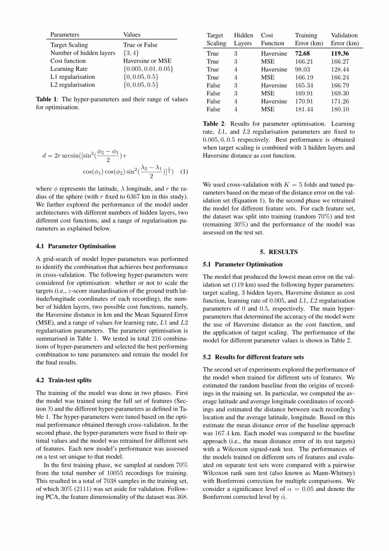
Target Scaling True or FalseNumber of hidden layers {3, 4}Cost function Haversine or MSELearning Rate {0.005, 0.01, 0.05}L1 regularisation {0, 0.05, 0.5}L2 regularisation {0, 0.05, 0.5}

Table 1: The hyper-parameters and their range of valuesfor optimisation.

d = 2r arcsin([sin2(φ2 − φ1

2)+

cos(φ1) cos(φ2) sin2(λ2 − λ1

2)]

12 ) (1)

where φ represents the latitude, λ longitude, and r the ra-dius of the sphere (with r fixed to 6367 km in this study).We further explored the performance of the model underarchitectures with different numbers of hidden layers, twodifferent cost functions, and a range of regularisation pa-rameters as explained below.

4.1 Parameter Optimisation

A grid-search of model hyper-parameters was performedto identify the combination that achieves best performancein cross-validation. The following hyper-parameters wereconsidered for optimisation: whether or not to scale thetargets (i.e., z-score standardisation of the ground truth lat-itude/longitude coordinates of each recording), the num-ber of hidden layers, two possible cost functions, namely,the Haversine distance in km and the Mean Squared Error(MSE), and a range of values for learning rate, L1 and L2regularisation parameters. The parameter optimisation issummarised in Table 1. We tested in total 216 combina-tions of hyper-parameters and selected the best performingcombination to tune parameters and retrain the model forthe final results.

4.2 Train-test splits

The training of the model was done in two phases. Firstthe model was trained using the full set of features (Sec-tion 3) and the different hyper-parameters as defined in Ta-ble 1. The hyper-parameters were tuned based on the opti-mal performance obtained through cross-validation. In thesecond phase, the hyper-parameters were fixed to their op-timal values and the model was retrained for different setsof features. Each new model’s performance was assessedon a test set unique to that model.

In the first training phase, we sampled at random 70%from the total number of 10055 recordings for training.This resulted in a total of 7038 samples in the training set,of which 30% (2111) was set aside for validation. Follow-ing PCA, the feature dimensionality of the dataset was 368.

Target Hidden Cost Training ValidationScaling Layers Function Error (km) Error (km)

True 3 Haversine 72.68 119.36True 3 MSE 166.21 166.27True 4 Haversine 98.03 128.44True 4 MSE 166.19 166.24False 3 Haversine 165.34 166.79False 3 MSE 169.91 169.30False 4 Haversine 170.91 171.26False 4 MSE 181.44 180.10

Table 2: Results for parameter optimisation. Learningrate, L1, and L2 regularisation parameters are fixed to0.005, 0, 0.5 respectively. Best performance is obtainedwhen target scaling is combined with 3 hidden layers andHaversine distance as cost function.

We used cross-validation with K = 5 folds and tuned pa-rameters based on the mean of the distance error on the val-idation set (Equation 1). In the second phase we retrainedthe model for different feature sets. For each feature set,the dataset was split into training (random 70%) and test(remaining 30%) and the performance of the model wasassessed on the test set.

5. RESULTS

5.1 Parameter Optimisation

The model that produced the lowest mean error on the val-idation set (119 km) used the following hyper parameters:target scaling, 3 hidden layers, Haversine distance as costfunction, learning rate of 0.005, and L1, L2 regularisationparameters of 0 and 0.5, respectively. The main hyper-parameters that determined the accuracy of the model werethe use of Haversine distance as the cost function, andthe application of target scaling. The performance of themodel for different parameter values is shown in Table 2.

5.2 Results for different feature sets

The second set of experiments explored the performance ofthe model when trained for different sets of features. Weestimated the random baseline from the origins of record-ings in the training set. In particular, we computed the av-erage latitude and average longitude coordinates of record-ings and estimated the distance between each recording’slocation and the average latitude, longitude. Based on thisestimate the mean distance error of the baseline approachwas 167.4 km. Each model was compared to the baselineapproach (i.e., the mean distance error of its test targets)with a Wilcoxon signed-rank test. The performances ofthe models trained on different sets of features and evalu-ated on separate test sets were compared with a pairwiseWilcoxon rank sum test (also known as Mann-Whitney)with Bonferroni correction for multiple comparisons. Weconsider a significance level of α = 0.05 and denote theBonferroni corrected level by α.

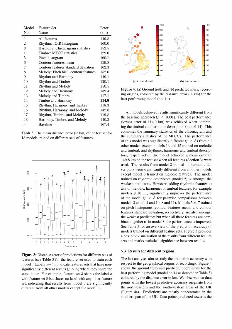
Model Feature Set ErrorNo. Name (km)

1 All features 149.82 Rhythm: IOIR histogram 160.03 Harmony: Chromagram statistics 152.54 Timbre: MFCC statistics 129.05 Pitch histogram 160.16 Contour features mean 159.87 Contour features standard deviation 162.38 Melody: Pitch hist., contour features 152.69 Rhythm and Harmony 149.110 Rhythm and Timbre 120.111 Rhythm and Melody 150.512 Melody and Harmony 139.413 Melody and Timbre 117.114 Timbre and Harmony 114.015 Rhythm, Harmony, and Timbre 118.316 Rhythm, Harmony, and Melody 142.817 Rhythm, Timbre, and Melody 119.818 Harmony, Timbre, and Melody 140.3

– Baseline 167.4

Table 3: The mean distance error (in km) of the test set for18 models trained on different sets of features.

1 2 3 4 5 6 7 8 9 10 12 14 16 18

010

020

030

040

0

f

h

a bc

h

h h

af

f

g

f ce

dg

d

dg

ce

bg

e

Feature sets

Dis

tanc

e er

ror

(km

)

Figure 3: Distance error of predictions for different sets offeatures (see Table 3 for the feature set used to train eachmodel). Labels a−l in indicate features sets that have non-significantly different results (p > α) where they share thesame letter. For example, feature set 3 shares the label awith feature set 8 but shares no label with any other featureset, indicating that results from model 3 are significantlydifferent from all other models except for model 8.

0

100

200

300

400

500

600

700

800

900

1000

(a) Ground truth

0

100

200

300

400

500

600

700

800

900

1000

(b) Predictions

Figure 4: (a) Ground truth and (b) predicted music record-ing origins, coloured by the distance error (in km) for thebest performing model (no. 14).

All models achieved results significantly different fromthe baseline approach (p < .0001). The best performance(lowest error of 114.0 km) was achieved when combin-ing the timbral and harmonic descriptors (model 14). Thiscombines the summary statistics of the chromagram andthe summary statistics of the MFCCs. The performanceof this model was significantly different (p < α) from allother models except models 13 and 15 trained on melodicand timbral, and rhythmic, harmonic and timbral descrip-tors, respectively. The model achieved a mean error of149.8 km on the test set when all features (Section 3) wereused. The results from model 3 trained on harmonic de-scriptors were significantly different from all other modelsexcept model 8 trained on melodic features. The modeltrained on rhythmic descriptors (model 2) is amongst theweakest predictors. However, adding rhythmic features toany of melodic, harmonic, or timbral features, for examplemodels 9, 10, 11, significantly improves the performanceof the model (p < α for pairwise comparisons betweenmodels 3 and 9, 4 and 10, 8 and 11). Models 5, 6, 7 trainedon pitch histograms, contour features mean, and contourfeatures standard deviation, respectively, are also amongstthe weakest predictors but when all these features are com-bined together as in model 8, the performance is improved.See Table 3 for an overview of the prediction accuracy ofmodels trained on different feature sets. Figure 3 providesa box-plot visualisation of the results from different featuresets and marks statistical significance between results.

5.3 Results for different regions

The last analyses aim to study the prediction accuracy withrespect to the geographical origins of recordings. Figure 4shows the ground truth and predicted coordinates for thebest performing model (model no.14 as denoted in Table 3)coloured by the distance error in km. We observe that datapoints with the lowest predictive accuracy originate fromthe north-eastern and the south-western areas of the UK(Figure 4a). Predictions are mostly concentrated in thesouthern part of the UK. Data points predicted towards the

0

100

200

300

400

500

600

700

800

900

1000

(a) Rhythm

0

100

200

300

400

500

600

700

800

900

1000

(b) Harmony

0

100

200

300

400

500

600

700

800

900

1000

(c) Timbre

0

100

200

300

400

500

600

700

800

900

1000

(d) Melody

Figure 5: Music recording origins coloured by the distance error (in km) for models trained on (a) rhythmic, (b) harmonic,(c) timbral, and (d) melodic features (models no. 2, 3, 4, 8 respectively as defined in Table 3).

eastern areas indicate a larger distance error (Figure 4b).In Figure 5 we visualise the prediction accuracy of mod-

els trained on different feature sets with respect to geogra-phy. We observe that for all models the northern areas ofthe UK (i.e., in the region of Scotland) are predicted witha relatively large distance error (lowest accuracy). For themodel trained on timbral features (Figure 5c) we also ob-serve the south west of England predicted with lower ac-curacy than the models trained on harmonic and melodicfeatures (Figures 5b and 5d).

6. DISCUSSION

Our results provide insights on the contribution of differentfeature sets and suggest patterns of music similarity acrossgeographical regions. The methodology can be improvedin various ways.

The initial corpus of folk and traditional music from theUK consisted of a total of 17000 of which only 10055were processed in this study. The final dataset had askewed geographical distribution with over-representationof the south-eastern and south-western UK regions, e.g.,Devon and Suffolk, and under-representation of the North-Eastern, North-Western areas, e.g., Scotland and NorthernIreland. Effects from the skewness of the dataset could beobserved in the distribution of predicted latitude and longi-tude coordinates (Figure 4b). A larger and more represen-tative corpus can be used in future work.

We used features derived from the output of VAMP plu-gins to describe musical content of audio recordings. Someof these plugins were designed for different music stylesand their application to folk music might not give robustresults. A thorough evaluation of the suitability of thefeatures can give valuable insights for improving their ro-bustness to different corpora such as the one used in thisstudy. We used feature representations averaged over timebut in future work preserving temporal information in thefeatures could provide better music content description.

We observed that results from models trained on indi-vidual features showed on average larger distance errors.When however combinations of features were considered,the model achieved on average higher accuracies. An ex-ception is the case when all features were considered butthe performance of the model had a relatively large dis-

tance error. This could be due to limitations of the modelespecially with regards to over-fitting or the lack of ade-quate music information captured by the features. Inte-grating additional audio features could help capture moreof the variance of the data and improve the model.

The model was validated for a range of parameters andseveral approaches were considered to avoid over-fitting.However, evidence of over-fitting could still be observedin the final results. Training with more data could helpmake the model more generalisable in future work. What ismore, oversampling techniques could be explored to over-come the problem of under-represented geographical re-gions in our dataset.

Neural networks in combination with audio features asproposed in this study, can provide good predictions of theorigins of the music. This can aid musicological researchas well as improve spatial metadata associated with largemusic collections.

7. CONCLUSION

We studied a collection of field recordings from theUK and investigated whether the geographical origins ofrecordings can be predicted from the music attributes ofthe audio signal. We treated this as a regression prob-lem and trained a neural network to take as input audiofeatures and predict the latitude and longitude of the mu-sic’s origin. We trained the model under different hyper-parameters and tested its performance for different featuresets. Highest accuracy was achieved for the model trainedon timbral and harmonic features but no significant differ-ences were found to the same model with rhythm featuresadded or with melody replacing harmony. The southernregions of the UK were predicted with a relatively high ac-curacy whereas northern regions were predicted with lowaccuracy. Effects of the skewness of the dataset and the re-liability of audio features were discussed. The corpus andmethodology can be improved in future work and the ap-plicability of the model could be extended to music fromaround the world.

8. ACKNOWLEDGEMENTS

MP is supported by a Queen Mary research studentship.

9. REFERENCES

[1] S. Abdallah, E. Benetos, N. Gold, S. Hargreaves,T. Weyde, and D. Wolff. The Digital Music Lab: ABig Data Infrastructure for Digital Musicology. ACMJournal on Computing and Cultural Heritage, 10(1),2017.

[2] J. Eisenstein, B. O’Connor, N.A Smith, and E.P. Xing.A Latent Variable Model for Geographic Lexical Varia-tion. In Proceedings of the 2010 Conference on Empir-ical Methods in Natural Language Processing, pages1277–1287, 2010.

[3] E. Gomez, M. Haro, and P. Herrera. Music and geog-raphy: Content description of musical audio from dif-ferent parts of the world. In Proceedings of the Inter-national Society for Music Information Retrieval Con-ference, pages 753–758, 2009.

[4] F. Gouyon, S. Dixon, E. Pampalk, and G. Widmer.Evaluating rhythmic descriptors for musical genre clas-sification. In Proceedings of the AES 25th InternationalConference, pages 196–204, 2004.

[5] C. Harte and M. Sandler. Automatic chord identifca-tion using a quantised chromagram. In 118th Audio En-gineering Society Convention, 2005.

[6] J. Inman. Navigation and Nautical Astronomy: For theUse of British Seamen. F. & J. Rivington, 1849.

[7] I. Karydis, K. Kermanidis, S. Sioutas, and L. Iliadis.Comparing content and context based similarity formusical data. Neurocomputing, 107:69–76, 2013.

[8] B. Logan. Mel-Frequency Cepstral Coefficients forMusic Modeling. In Proceedings of the InternationalSymposium on Music Information Retrieval, 2000.

[9] M. Marolt. Music/speech classification and detectionsubmission for MIREX 2015. In MIREX, 2015.

[10] M. Mauch, R. M. MacCallum, M. Levy, and A. M.Leroi. The evolution of popular music: USA 1960-2010. Royal Society Open Science, 2(5):150081, 2015.

[11] C. McKay and I. Fujinaga. Automatic genre classifi-cation using large high-level musical feature sets. InProceedings of the International Society for Music In-formation Retrieval Conference, pages 525–530, 2004.

[12] D. Moelants, O. Cornelis, and M. Leman. ExploringAfrican Tone Scales. In Proceedings of the Interna-tional Society for Music Information Retrieval Confer-ence, pages 489–494, 2009.

[13] B. Nettl. The Study of Ethnomusicology: Thirty-one Is-sues and Concepts. University of Illinois Press, Urbanaand Chicago, 2nd edition, 2005.

[14] B. Nettl, R. M. Stone, J. Porter, and T. Rice, editors.The Garland Encyclopedia of World Music. GarlandPub, New York, 1998-2002 edition, 1998.

[15] J. Novembre, K. Bryc, S. Bergmann, A.R. Boyko,C.D. Bustamante, A. Auton, M. Stephens, Z. Kuta-lik, A. Indap, T. Johnson, M.R. Nelson, and K.S.King. Genes mirror geography within Europe. Nature,456(7218):98–101, 2008.

[16] M. Panteli, R. Bittner, J. P. Bello, and S. Dixon. To-wards the characterization of singing styles in worldmusic. In IEEE International Conference on Acoustics,Speech and Signal Processing, pages 636–640, 2017.

[17] P. E. Savage and S. Brown. Mapping Music: Clus-ter Analysis Of Song-Type Frequencies Within andBetween Cultures. Ethnomusicology, 58(1):133–155,2014.

[18] P. E. Savage, S. Brown, E. Sakai, and T. E. Currie.Statistical universals reveal the structures and func-tions of human music. Proceedings of the NationalAcademy of Sciences of the United States of America,112(29):8987–8992, 2015.

[19] D. Turnbull and C. Elkan. Fast recognition of musi-cal genres using RBF networks. IEEE Transactionson Knowledge and Data Engineering, 17(4):580–584,2005.

[20] G. Tzanetakis, A. Ermolinskyi, and P. Cook. Pitch his-tograms in audio and symbolic music information re-trieval. Journal of New Music Research, 32(2):143–152, 2003.

[21] W. Yang, J. Novembre, E. Eskin, and E. Halperin. Amodel-based approach for analysis of spatial structurein genetic data. Nature Genetics, 44(6):725–731, 2012.

[22] J. M. Young, L. S. Weyrich, J. Breen, L. M. Mac-donald, and A. Cooper. Predicting the origin of soilevidence: High throughput eukaryote sequencing andMIR spectroscopy applied to a crime scene scenario.Forensic Science International, 251:22–31, 2015.

[23] F. Zhou, Q. Claire, and R. D. King. Predicting the Geo-graphical Origin of Music. In IEEE International Con-ference on Data Mining, pages 1115–1120, 2014.