geodetic aspects of engineering surveys requiring … · geodetic aspects of engineering surveys...
TRANSCRIPT

GEODETIC ASPECTS OF ENGINEERING SURVEYS
REQUIRING HIGH ACCURACY
BILL TESKEY
September 1979
TECHNICAL REPORT NO. 65

PREFACE
In order to make our extensive series of technical reports more readily available, we have scanned the old master copies and produced electronic versions in Portable Document Format. The quality of the images varies depending on the quality of the originals. The images have not been converted to searchable text.

GEODETIC ASPECTS OF ENGINEERING SURVEYS REQUIRING HIGH ACCURACY
Bill Teskey
Department of Surveying Engineering University of New Brunswick
P.O. Box 4400 Fredericton, N .B.
Canada E3B 5A3
September 1979 Latest Reprinting June 1993

PREFACE
This report is an unaltered version of the author's
masters thesis of the same title.
The thesis advisers under whom this work was
carried out were Dr. Adam Chrzanowski and Dr. Klaus-Peter
Schwarz. Acknowledgement of the assistance rendered by
others is given in the Acknowledgeme~ts.

ABSTRACT
Nany of today's engineering surveys require relative
positional accuracies in the order of 1/100 000 or better. This means
that positional observations must be very accurate, ancl that a rigor
ous geodetic approach must be followed.
This thesis is directed tov1ard the geodetic aspect. Chapter
2 reviews the geodetic models and coordinate systems available. For
an engineering survey requiring high relative positional accuracy a
local p_lane coordinate system and a geodetic height system, both
based on the classical geodetic model, is the appropriate choice.
Chapter 3 reviews the well known geometric and gravimetric effects in
a local coordinate system.
Specia·l emphasis is placed on methods to determine deflections
of the vertical in chapter 4. It was felt that a contribution could be
made if a simple method could be developed to determine deflections,
which describe variations in the gravity field. (Very often the
effect of variations in the gravity field on survey observations are
neglected only because they are difficult to determine,') Such a
method was developed by the author by applying a difference method to
the usual astrogeodetic deflection determination. The method is very
simple and practical, and field test results indicate it is accurate
i i
to 1" to 2". Extensive field work associated with the use of
trigonometric levelling to determine local deflections led to
inconclusive results because the effect of vertical refraction
could not be isolated.
Chapter 5 shows the application of the material presented
in the first four chapte"s, Nith emphasis on the effect of deflection
of the vertical. The two problems considereu show that often, even
for engineering surveys requiring high accuracy, the effect of
variations in the earth•s gravity field can be safely neglected. This
however can only be determined by analyzing each problem using
accurate deflection components to estimate the effect in the horizontal
and a small number of gravity values to estimate the effect on heights.
Being able to easily-define the local gravity field a priori
by the astrogeodetic difference method will probably have its best
application in situations in which the local variations have their
greatest effect, for example in the determination of heights in a three
dimensional conrdinate system and in the determination of horizontal
· positions with inertial surveying systems.
iii

ABSTRJl.CT . . . • • •
TABLE OF CONTENTS
LIST OF 'FIGURES .
LIST OF TABLES .•
ACKNOWLEDGEMENTS.
1. INTRODUCTION
TABLE OF CONTENTS
1.1 General • • . . . . . . . . . ....• 1.2 Engineering Surveys and an In~egrated Survey
ii
iv
vii
ix
X
System . , . . . . . . . . . . . . . . 2
2. A GEODETIC MODEL AND COORDINATE SYSTEf~ 5
2.1 Choices of Geodetic Models .....
2.1. 1 2.1.2 2. 1. 3 2. 1. 4
Time Varying Model ..... . Contemporary Three-Dimensional Classical Geodetic Model .•• The Choice of a Geodetic Model En~i neeri ng Survey . • o • • •
Model .
for an
2.2 The Classical Geodetic Model and a Local Coordinate
5
System o o • • • • • • • • • • • • •. • • • 17
2.2. 1 Establishment of a Horizontal Datu~ 19 2.2.2 A Plane Coordinate System . . . . . . 24 2.2.3 A Geodetic Height D~tum ... , . . . 25
3. GEOMETRIC AND GRAVIMETRIC EFFECTS IN A LOCAL COORDINATE SYSTEM • • . . . . . . . . . 27
3.1 Heights ........... o o 0 28 3.2 Horizontal Positioning . . . . . . 32
iv

3.2.1 Reduction of Observations from Terrain to Ellipsoid . . . . . . . . . . . . . . . . . 35
3.2. 1.1 Reduction of Spatial Distances . . . 35 3.2.1.2 Reduction of Astronomic Azirr.uths . . 38 3.2~1.3 Reduction of Horizontal Directions 39 3.2.1.4 Reduction of Horizontal Angles.· .· 39 3.2.1.5 Magnitude of the torrections . . . 4Q
3.2.2 Reduction of Observations from Ellipsoid to Transverse Mercator Conformal Mapping Plane 45
3.2.2.1 Reduction of Ellipsoid Distances·. 3.2.2.2 Reduction of Geodetic Azimuths .. 3.2.2.3 Reduction of Horizontal D~rections 3.2.2.4 Reduction of Horizontal Angles . 3.2.2.5 Magnitude of the Corrections ...
4. DETERMINATIO~ OF DEFLECTIONS OF THE VERTICAL
4.1 Review of Existing Methods ..... . . ..
46 48 49 49 . 50
54
55
4.1.1 Trigonometric Method ..... · 55 4.1.2 Astrogeodetic Method • . . . . . . • . 58 4. 1. 3 .Gra vi metric Method • · . · . . • . . . . . . . 58 4. 1. 4 T apograph i c ~1e thad . . . . . . • . . . . . 60 4. 1. 5 Combined Method (Least .Squares ·Colloc-ation· ~1ethod)53 4.1.6 ·Inertial Method . . . . . 64
4.2 Astrogeodetic Difference Method
4.2.1 Description ..... . 4.2.2 A Priori Error Analysis .
4.3 Field Tests ..... .
4.3. 1 Frederi c.ton Area
65
65 71
75
76
4.3.1. 1 Use of the Trigonometric Method. . 78 4.3.1.2 Use of the Astrogeodetic Difference
~ethod • . . . . . . . . • 82 4.3.1.3 Comparison of the Results . . . . . 88
4.3.2 Fundy Park Area . . . . . . . . . . . . . . 88
v

5. APPLICATION TO ENGINEERING SURVEYS .
5.1 A Simulated Tunnel Survey .•
94
94
. 5. 1.1 Lateral Breakthrough Error • • 95 5.1.2 Vertical Breakthrough Error . . . . . • . . 102 5.1.3 The Effect of Neglecting.the Gravity Field 106r
5.2 Alignment of a Straight Line in Space . 109
6. CONCLUSICNS AND RECOM~1E"lDATIONS • 115
REFERENCES 119
APPENDIX I •
APPENDIX II
vi
. . . 125
127

LIST OF FIGURES
Figure 2-1 Ellipsoidal {~, X, h) and Geodetic Cartesian {XG, YG, ZG) Coordinates •.•.•.•... . . . . . 10
Figure 2-2 The Local Three-Dimensional Cartesian Coordinate System • • . . • . • • . . . . • • • • • • 18
;.igure 2-3 A Geocentric ~eference Ellipsoid .•
Figure 2-4 A Nongeocentric Reference Ellipsoid
. . . .
Figure 3-1 Ellipsoid and Conformal Mapping Plane for a National
21
21
Geodetic Network •••..•. _ . . • . • • • • • • • . . . 34
Figure 3-2 Ellipsoid and Conformal Mapping Plane for a Local Geodetic Network . • • • .
Figure 3-3 Spatial Diitance Reduction .
Figure 3-4 Slope Correction •••.
Figure 3-5 Gravimetric Cor1·ection •.
Figure 3-6 s~ew Normal Correction ••.
Figure 3-7 Normal Section to Geodesic Correction.
Figure 3-8 Geometry of Projected Curves •.••.•
Figure 3-9 Scale.Factor Correction (Transverse Mercator Projection) . . . • .•.•...•....•
Figure 3-10 Meridian Convergence Correction (Transverse Mercator Projection) • • • • . • • • • • • • • . • .
. .
. .
. .
34
36
41
. . 42
43
44
47
. - . 51
. . 52
Figure 3-11 (T -t) Correction (Transverse Mercator Projection) • • 53
Figure 4-1 Effect of Topography on Deflection of the Vertical •.••. 62
Figure 4-2 Basic Concept of Measurement of Change in Deflection by an ISS . . • . • • • . • . . . • . • . • . • . . . . . 65
Figure 4-3 Deflections of the Vertical in the Fredericton Area by the Astrogeodetic Difference Method • . • . • • • • . . 77
vii

Figure 4-4 Deflections of the Vertical in the Fundy Park Area . 89
Figure 5-1 Horizontal Control for a Simulated Tunnel Survey .• 96
Figure 5-2 The Vertical Component of Alignment of a Straight Line in Spree ..•.•••••..••.•••.•. 112
viii
LIST OF TABLES
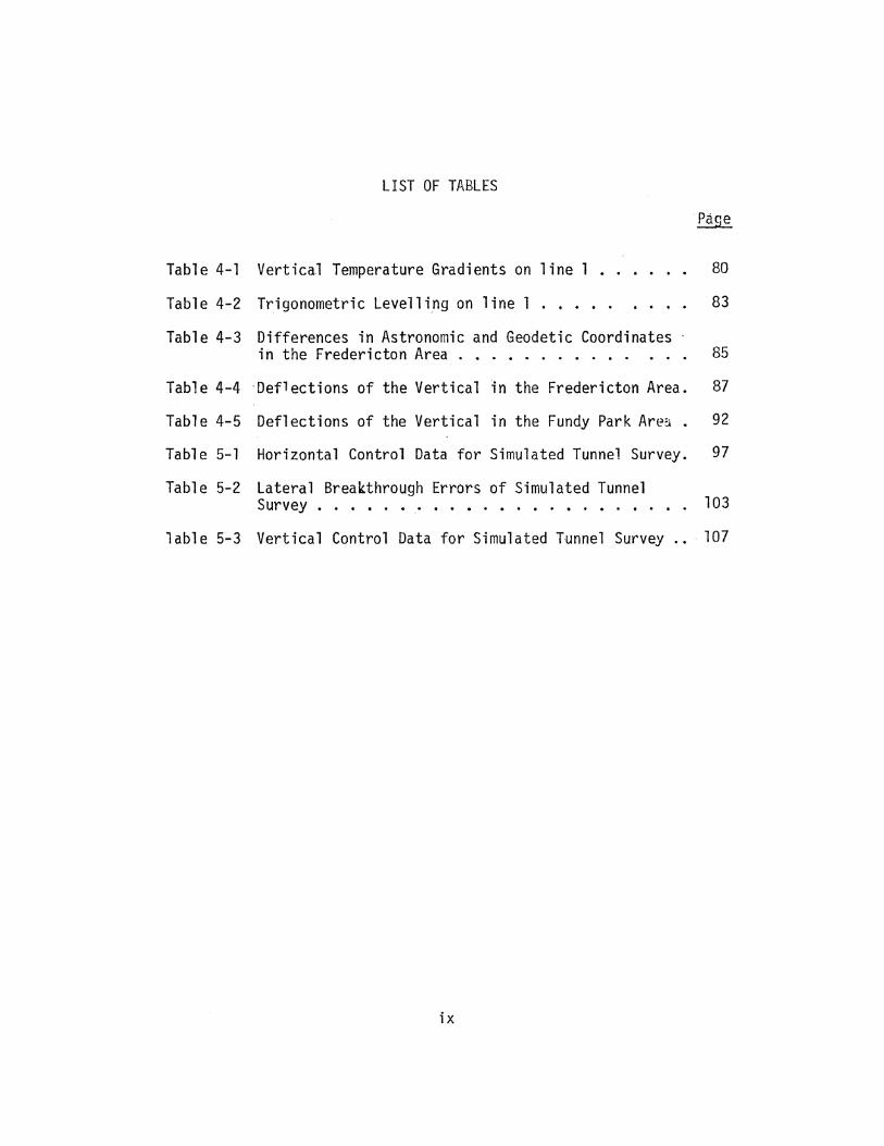
Table 4-1 Vertical Temperature Gradients on line 1 ..
Table 4-2 Trigonometric Levelling on line 1
Table 4-3 Differences in Astronomic and Geodetic Coordinates
80
83
in the Fredericton Area . . . • . . . • . . . 85
Tabie 4-4 ·Deflections of the Vertical in the Fredericton Area. 87
Table 4-5 Deflections of the Vertical in the Fundy Park Are~ • 92
Table 5-l Horizontal Control Data for Simulated Tunnel Survey. 97
Table 5-2 Lateral Breakthrough Errors of Simulated Tunnel Survey . . . . . • . • . . . . . • . • . . 103
lable 5-3 Vertical Control Data for Simulated Tunnel Survey .• · 107
ix
ACKNOWLEDGEMENTS
I would l~ke to express my appreciation to Dr. Adam·chrzanowski,
my advis~r, for his unwavering support and encouragement. I would
also like to thank Dr. Klaus-Peter Schwarz and Dr. Gerard Lachapelle
for discussing the astrogeodetic difference method with me and
providing an independent solution with which to compare.
Many people are to be thanked for assisting me with the field
work. The students of Survey Camp III measured the length of line l.
The students of Survey Camp II' performed 20 km of precise spirit
ievelling, the quality of which would be difficult to surpass. Pablo
Romero, Julio Leal, Ashoki Sujanani, Conrad Saulis~and Derek Davidson
are to be especially thanked for giving freely of their time on .
clear cold nights this spring and summer when sensible people were at
home·in bed. Appreciation is gratefully extended to Mr. Winston
·Smith, Superintendent of Fundy'National Park,· for providing two-way
radio communication in the Fundy Park area.
Susan Biggar is thanked for her excellent job of typing this
thesis. Financial support received from the Department of Surveying
Engineering, University of New Brunswick is gratefully acknowledged.
Often moral support was more urgently required than material
support. When encouragement was needed, my fellow graduate students
and my family and friends at home.provided it.
X

1. INTRODUCTION
1.1 GenP.ral
Throughout history there has been a nted for engineering
surveys. The accuracy requirements of most were such that no special
effort or knowledge was r~quired to execute them. There were some
problems however. that taxed the best minds of the day; the setting
out of a long tunnel is the classic example. Today this same
problem would challenge the abilities of any.surveying engineer. Two
other exam:-'les of modern day projects requiring engineering surveys
of high accuracy are the setting out of nuclear accelerators and the
alignment of a straight line in space for the positioning of the
aerials of a radio telescope array.
Today's demand for engineering surveys of high accuracy has
been matched by advances in survey instrumentation. With the advent
of EDM, angles and distances can be measured with comparable accuracy;
with careful use of ro~tinely available equipment both can be measured
with an accuracy greater than 1/100 000. Using proper methods of
network design, measurement and adjustment, relative positional
accuracies of the same order can be attained.

2
If relative positional accuracies of the order of l/100 000
are actually to be atta ir.ed, a rigorous geodetic approach must be
follm'led. This means that for even small project are·as the effect of
the e 11 i psoi da 1 shape of the earth and the effect of the earth's
gravity field must be accounted for. Although th~s-e two effects are
inextricably linked, they are most often dealt with separately. In
this thesis the same approach will be ;·allowed.
Throughout this thesis reference to engineerin_g surveys
requiring high accuracy will imply relative positional accuracies in
the order of l/100 000 between locally stable points. Special
eng-ineering surveys concerned with the movements of points will not
be considered.
1.2 Engin~ering Surveys and an Integrated S~rveying System·
_Much work has been done in recent years to develop a workable
survey control frc.mework for position - related information at a
regional or national level. This survey control framework and the
position related information tied to it is generally referred to as
an integrated survey system.
In order for int~grated systems to_ operate for maximum
benefit all surveying and mapping activities should be tied.to them.
For routine engineerins surveys requiring relative positional accuracies
in the order of l/10 000, the survey control framework of integrated
survey systems could be used directly as control. For engineering
surveys requiring relative pGsitional accuracies in the order of l/100 000
or better, the survey control framework of integrated survey systems
might not be adequate.
3
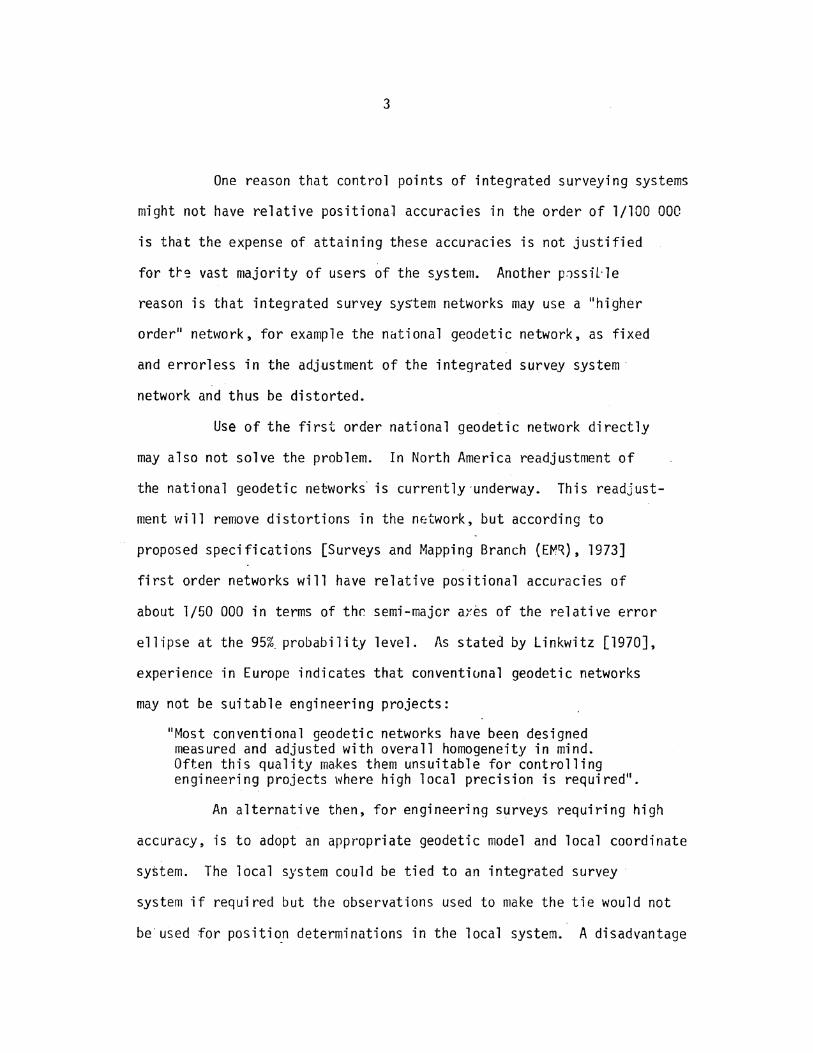
One reason that control points of integrated surveying systems
might not have relative positional accuracies in the order of l/100 000
is that the expense of attaining these accuracies is not justified
for tre vast majority of users of the system. Another p~ssiL·le
reason is that integrated survey sys-tem networks may use a "higher
order" network, for example the national geodetic network, as fixed
and errorless in the adJustment of the integrated survey system·
network and thus be distorted.
Use of the first order national geodetic network directly
may also not solve the problem. In North America readjustment of
the national geodetic networks· is currently-underway. This readjust-
ment will remove distortions in the network, but according to
proposed specifications [Surveys and Mapping Branch (EM~). 1973]
first order networks will have relative positional accuracies of
about l/50 000 in terms of thr. semi-majcr aYes of the relative error
ellipse at the 95%. probability level. As stated by Linkwitz [1970],
experience in Europe indicates that conventi0nal geodetic networks
may not be suitable engineering projects:
"Most conventional geodetic networks have been designed measured and adjusted with overall homogeneity in mind. Often this quality makes them unsuitable for controlling engineering projects 1'/here high local precision is required 11 •
An alternative then, for engineering surveys requiring high
accuracy, is to adopt an appr·opriate geodetic model and local coordinate
system. The local system could be tied to an integrated survey ·
system if required but the observations used to make the tie would not
be'used for positi~n determinations in the local system. A disadvantage
4
of this approach is that coordinates {and their accuracies) from
another coordinate system could not be utilized as additional information
for position determinations in the local system without a transfo~mation.
The use of coordinates as observations {additional 1nformation) is
discussed in ChrzanmoJski et al [1979] and Vanicek and Krakh-1sky [in
prep];
In revie\Jing the literature on engineering surveys requiring
high accuracy it was found that only rarely,outside of Europe, is this
approach followed. Often it seemed that only the mystique surrounding
geodesy prevented those responsible for the survey control from
attaining better accuracies.

2 .. A GEODETIC MODEL AND COORDINATE SYSTEM
2.1 Choices of Geodetic Models
A geodetic model of a set of points on the surface of the
earth consists of a definition of a coordinate system and its location
within the earth, and the coordinates of the points in this coordinate
system •.
Basically, there exist two different approaches to the
problem of geodetic positioning. One approach regards the points on
the surface of the earth as being perpetually in motion with respect
to each other as well as with respect to th~ coordinate system. In
this model the coordinates are therefore time varying and the model
is four dimensional: three coordinates specifying position, and
one coordinate specifying time. The other more conventional approach
treats the positions of the points as permanent with respect to
the coordinate system.
2.1.1 Time Varying Model
The ultimate goal in geodesy is to be able to provide
instantaneous positions of ground points as they vary with time
[Mather, 1974].
5

6
Ground, or more generally, surface movements can be due to
three effects. These three effects are earth tides, sea tides loading,
and aperiodic surface or crustal movements.
(i) The earth tides. This is a global phenomenon. It changes the
shape of the earth so that a point on the surface of the earth can
oscillate as much as -15 em to +30 em with respect to the center
of mass of the earth.
There is also an annual distortion of the earth's surface
caused partly by earth tides but mainly by atmospheriC variations.
Very little is known about the geodetic effects of this distortion.
(ii) Sea tides' loading. Sea tides are a more complex phenomenon
than earth tides. Only at tidal stations can sea tides by directly
measured, and in .order to predict the lJading at a point on the
surface of the earth, the distribution of sea tides mu~t be known
over a large area. In addition to this the elastic properties of
the earth's crust must be well known. For these reasons, the degree
of reliability in predicting distoritons caused by sea tides' loading
is low.
One sea tides loading prediciton gives a semi-diurnal (12
hour) loading effect in the immediate vicinity of ti1e Bay of Fundy
of several centimeters vertical. The associated grount tilt
is ahout 0~1. both of these effects fade waay inland. It
should also be noted that the sea tides' loading effect in this

7
area probably would be the largest experienced anywhere in the world
since the Bay of Fundy experiences the world's highest tides.
(iii) Aperiodic surface.or crustal movements. All other surface
movements have .bren lumped together i11to this category only because
they do not show a regular variation with time. These movements can
be further divided into movements due to crustal loading (other ~han
.sea tides' loading}, movements due to tectonic action, movements due
to man's activities and movements due to other causes.
Movements due to crustal loading are predominautly vertical
movements. The loading (or unloading) causing this movement may be
due to a large water reservoir, a large city, sediments depos.ited
or material eroded by a major river, post glacial isostatic rebound,
or other factors. Tectonic action refers to movements of large
plates of the earth's crust on the upper mantle material. These
movements have recently become the subject of vigorous resea~ch,
for example the movements associated with the San Andreas fault in
California. Movements due to man's activities could be ground
consolidation due to withdrawal of fluids such as oil or water, or
ground swelling due to fluid waste disposal. Man's activities
.,.C.ould also cau·se landslides,and subsidences following mining exploitation.
Movements due to other causes would include thermo-elastic deformations
of the earth, about which very little is known quantitatively, and
regional anomalous uplifts or subsidences of no immediately
explainable origin. An example of the latter is the vertical
movement in the Lac St. Jean area of Quebec [Vanicek and Hamilton, 1972].

Before concluding this discussion of surface movemerts, the.
long term movement of mean sea level should be mentioned )ecause mean
sea level is commonly used as a height datum. Studies have shown a
eustatic (world mean sea level) rise of the order of 10 em per century
[Holdahl, 1974].
2. 1.2 Contemporary Three-Dimensional Model
In this model the coordinate system is three-dimensional and
the positions of points are considered invariant ~ith time. This
approach is not new - it was first suggested by Bruns in 1878. The
formulae used in contemporary three-dimensional geodesy are generally
those contained· in Wolf [1963], Hirvonen [1964] or Hotine [1969] and
summarized in Heiskanen and Moritz [1967]. Many authors have refined
these or similar formulae and applied them to simulated or actual
networks. Examples are: Bacon [1966], Henderson [1968], Hradilek
[1968; 1972], Fubara [1969], Stolz [1972], Vincenty [1973], Vincenty
and Bowring [1978], Lehman [1979].
In recent years the three-dimensional approach has gained in
popularity. There are several reasons for this. One reason is that
surveying methods using photogrammetry, satellite receivers or inertial
systems are inherently three-dimensional. Another reasons is that the
computational requirements of simultaneously dea·ling with three
coordinates are no longer a problem due to advances in computer tech
nology. A third reason is that deflections of the vertical and geoid

9
heights, which can ~e used as input into the three-dimensional model
to obtain the most accurate values for the coordinates, can now be
better determined., (Deflections of the vertical and changes in geoid
heights express the variation of the earth•s gravity field. They also
affect the classical geodetic model, and this aspect is discussed in
deta~l in chapter 3.)
In the three-dimensional model the position of a point on tne
terrain is given by the ellipsoidal coordinates (~. A, h) or by the
geodetic cartesian coordinates (X6, v6, z6). ~ and A are taken as
positive to the north and east respectively. The geometric relationship
between these coordinates is indicated in Figure 2-1.
The ellipsoid height h is obtained by adding together the
orthometric height H and the geoid height N. A complete discussion
of the relationship between ellipsoidal and cartesian coordinates,
as well as other coordinate systems used in geodesy, is given in
Krakiwsky and Wells [1971].
2.1.3 Classical Geodetic Model
In th~ classical geodetic model, the triplet of coordinates
used to define the position of a point on-the surface of the earth are
separated into horizontal coordinates and a vertical coordinate. The
horizontal coordinates may be geodetic latitude ~ and geodetic longitude
A, or cartesian coordinates X and Y on a mapping plane. The vertical
coordinate is a rigorous geodetic height such as dynamic height or.
orthometric height.

10
Greenwich mean astronomic meridian
terrain
origin of geodetic A;---1-¥---.---+---------r---J- 7 Y G system /
A.
Figure 2-1
z l G
I / I /
/ /
/ XG
average terrestrial equator
Ellipsoidal (~, A., h) and Geodetic Cartesian (XG' YG' ZG) Coordinates
11
The main reason for the separation of coordinates is purely
practical. Horizontal geodetic stations, in order to be intervisible
so that-the traditional surveying measurements can be made, are
generally located on hilltops. Precise godet.c levelling between
these stations is usually very difficult and is very seldom perform~d
[Krakiwsky and Thomson; 1974]. Vertical control points, on the other
hand, are generally located along roads to that the levelling route is
easily accessible.
2.1.4 The Choice of a Geodetic Model for an Engineering Survey
The time-varying model would only be an appropriate choice
~or special engineering surveys concerned with the movements of points.
These types of surveys will not be considered in this thesis.
Movements due to earth-tides and sea tides• loading can cause
movements with respect to the center of mass of the earth in the order
of centimeters, but the relative changes in angles and distances in
the area covered by an engineering project are very small - of the order
of 10-8 [~1elchior, 1966] and undetectable with present surv.:ying. instru
ments. Relative movements due to crustal loading are of the same or~er.
Movements due to some of the remaining causes, for example tectonic
action and man•s activities, and anomalous movements could easily be
large enough so that terrain points could not be used for local control
purposes. In these cases terrain points would have to be carefully
chosen so that they would be locally stable.
The choice of a geodetic model for an engineering survey has
been reduced to either a three-dimensional model or the classical model.
The choice between thec;e two will take a little more consideration, for

12
each model has a number of distinct advantages and disadvantages.
One of the advantages of a three-dimensional model is that
observations do not have to be reduced to a reference surface. Only
the usual atmospheric and irstr~:nental corrections are made to the
observations.
Another advantage of the three-dimensional model is that
all three coordinates are determined for every point; however, for an
engineering project this advantage might not be utilized. Just as
design, measurement and adjustment of separate horizontal and vertical
networks is a practical procedure, it is .also a practical procedure
to set out heights from vertical control and horizontal positions from
horizontul control.
A third advantag~ of the three-dimensional model is that.it
can fully utilize satellite data. The three-dimensional model can
?lso utilize the output of other systems that operate ir. three~dimensional
space, for example photogrammetric systems [El Hakim, 1979] and inertial
survey systems.
The fact that in a·thre~-dimensional·model the three
coordinates are solved for simultaneously, leads to certain difficulties.
The most obvious difficulty is that a larger system of equations must
be solved. Another difficulty is that in a three-dimensional-model the
formulation of observation equations must be done in the ellipsoidal
coordinate system since horizontal directions (or angles) and zenith
angles cannot be expressed completely in cartesian coordinates
[Hotine, 1969; Chovitz, 1974].

13
Neither of these difficulties however, should be considered as
serious because of the computer facilities available today.
The most serious difficulty with a three-dimensional model
is that a height cooruinate is solved for at every point. This
requires additional ob5ervations. Spatial distances, except where
lines of sight are very steep, do little to accurately determine
heights [Hradilek, 1968]. Measurement of tt-e spatial distance
between two points together with the zenith angles corrected for
deflections of the vertical allow·differences of ellipsoid heights
to be calculated. These observations are essential for a three
dimensional geodetic model but, by themselves, are not sufficient
to determine the height coordinates as accurately as the horizontal
coordinates. Observations of astronomic latitude and astronomic
longitude and observations of differences in spirit levelled heights
are necessary to increase the accuracy of thE. heig:1t coo··dinates
[Fubara, 1969; Vincenty, 1973]. (These observations provide
information on the variation of the earth's gravity field between
points in the network. The role of astronomic observations and
observation~ of changes in height are discussed in detail in chapters
3 and 4}. Even with these additional observations the height coordin
ates may not be of the same accuracy as the horizontal coordinates.
This is because of the uncertainty associated with vertical refraction.
For smaller scale three-dimensional networks, such as those used to

14
determine ground movements, the uncertainty associated with vertical
refraction still has a significant effect [Dodson, 1978].
Vertical refraction can be treated as an unknown parameter
in a three-dimensional adjustment [Hradil~k, 1J72; Ramsayer, 1978]
but only with special observing methods, for example simultaneous
reciprocal zenith angles, or under special conditions, for example
lines high abrve the ground, can vertical refraction and heights be
well determined. An alternative to treating vertical refroction as
an unknown parameter is ta input it as a kno\'m quantity, but the
difficulty of adequately modelling vertical refraction is \vell
illustrated by the work of Angus-Leppan [1967; 1978], Brunner [1977]
and others.
Another alternative to treating vertical refr.action as an
unknown parameter may be available in th~ future. Work is currently
being carried cut by Tengs"':rcm [1977] at UppsalC~ University in Sweden
and by ~!ill iams [1977] at the National Physical Laboratory in England -I
on instruments to determine refraction directly by measuring the
· dispersion of two colours of 1 ight. (Vertical refraction is dealt
with in more detail in chapter 4 in connection with determination of
deflection of the vertical;)
The disadvantages of the classical geodetic model, especially
when applied to an engineering survey, are minor.
One disadvantage is that observations have to be reduced from
the terrain to the ellipsoid to the mapping plane. Since these
reductions are performed together with the atmospheric and instrumental

15
corrections, most likely within a co~·puter program, it cau~es no real
problem. The reductions due to gravity can be determined by a global
geoid model or, with more accuracy, by any of the methods outlined in Chapter 4.
Another disadvahtage of the classical geodetic model is that
horizontal control points have accurate horizontal coordinates but
only approximate heights, and vertical control points have accurate
heights but only approximate horizontal coordinates. Again, this
causes nc real problem. Just as design, measurement and a~justment of
separate horizontal and vertical networks is a practical procedure, it
is also a practical procedure tb set out heights from vertical control
and horizontal positions from horizontal control.
A third disadvantage of the classica 1 geodetic model is that
it cannot fully utilize three-dimensional data such as satellite data.
This is a very real disadvantage for national geodetic networks, but
is not a mu.jor consideration for most· engineering surveys requiring high.
accuracy. The reason for this is that in a small area, like that
covering an engineering project, three-dimensional data (satellite,
photogrammetric or inertial) is generally not sufficient to produce
horizontal and vertical positional accuracies of l/100 000; this
is especially true for the heights. For small areas the traditional
surveying measurements still provide the highest positional
accuracies. An except1on to this would be the positional accuracies.
of some satellite solutions, for exam~le the short arc satellite
solution in which accuracies of 0.25 m in all three coordinates
are claimed [Brown, 1976]. If some of the control for an
engineering survey were to be established by satellite methods, a datum
shift would be required to make the satellite derived coordinates

16
compatible with the coordinates derived from the traditional surveying
methods. (The reasons for the datum shift is explained in section 2.2.1.)
In this case the datum shift could be performed by a method outlined by
Merry and Vanicek [1974]. A few special engineering surveying problems
would be very difficult without satellite position determinat~ons;
Examples are the positioning and orientation of nuclear accelerators
and radio telescopes in which "absclute" position and "absolute" orient
ation (position with respect to the center of mass of the earth and
orientation with respect to the best-fitting geocentric ellipsoid -
see section 2.2.1) are necessary.
·The advantages of the classical geodetic model are due to practical
considerations. The classical geodetic model minimizes the effect of
atmospheric refraction by separating horizontal and vertical control. This
enables positional accuracies of l/100,000 to be attained. As has been
discussed previously, it is also very practical to deal with horizontal and
vertical control networks separately, and to set out from these networks separately
Another practical aspect of the classical. geodetic model is it height
component. In the classical geodetic model, he_ights whether dynamic or
orhtometric, have a definite physical meaning. Points having the same dynamic
height lie on the same equipotential surface. ·Points having the same ortho
metric·height are the.sa~e height above the geoid. ·(Heights will be discussed
in more detail in. chapter 3.} In the three-dimensional geodetic model, the
height ·component is either the local cartesian coordinate ZL or the ellipsoid
height h. Figure 2-2 shows the position and orientation of a local three
dimensional cartesian coordinate system. Given the parameters defining the shape
and position of the reference ellipsoid, ZL can be transformed to h and vice versa.
Ellipsoid height h is related to orthometric height H by the f6rnula h = H + N
(see section 2.1.2) but it is difficu1t to obtain an accurate value for Nat
a given point.

17
For engineering purposes neither ZL or hi~ very useful. If
heights on a given project were defined by zL•s it would cause a great
deal of confusion. By studying Figure 2-2, one can see that depending
on the location of points with resper.t to the origin of the local three
dimensional cartesian coordinate system a point with a larger ZL value
than another point may or may not be higher than the other point! Use
of ellipsoid heights would be bett2r but still not saiisfactory.
Changes in ellipsoid heights approximate changes in dynamic or ortho
metric heights but for engineering surveys requiring high accuracy,
especially in areas where variations in the gravity field are large,
use of ellipsoid heights would not be satisfactory.
The classical geodetic model has been in use since man fil·st
began to investigate the size and shape of the earth. It is still in
use today in all the national geodetic netwat~ks of the world. Despite
advances in all areas of surveying-new equipment and methods, more
dense coverage of data, the ability to rigorously adjust networks- the
classical geodetic model remains the most practical and useful. For
these reasons the classical geodetic model should be used in preference
to the three-dimensional geodetic model for·an engineer1ng survey
requiring high accuracy.
2.2. The Classical Geodetic Model.and a Local Coordinate System
In this section well known features of ·-horizontal and vertical
geodetic networks are reviewed. Definitions are kept to a minimum.
No references are given to formulae as these are readily available from

azimuth of XL axis
origin of geodetic system
18
Figure· 2-2
direction of .astronomic north
direction of local gravity
reference ellipsoid
The Local Three~Dimensional Coordinate System

19
any textbook on geodesy, for example Bamford [1975] and Vanicek and
Krakiwsky [in prep].
In the classical geodetic model the horizontal position of a
point is defined by geodetic latitude and long;tude on the surface of
a reference ellipsoid or by cartesian coordinates X andY on a mapping
plane. The vertical position in a classical geodetic model is defined
by a rigorous geodetic height.
For local control purposes two-dimensional· cartes-ian coordinates are
preferable to geodetic coordinates. Cartesian coordinates are most easily obtainec
by reducing horizontal position observations to the mapping plane and
then adjusting the reduced observations on the mapping plane. Before
this can be done however, a horizontal geodetic datum must be established.
2.2.1 Establishment of a Horizontal Geodetic Datum
A horizontal geodetic datum is simply the surface of the
reference ellipsoid. There are several ways in which a datum can be
defined. The classical approach is to determine a set of parameters
which define the datum, by making measurements on the sur.face of the
earth. This is the approach that will be followed here.
A set of eight parameters which define a horizontal geodetic
datum are: a, f, cp0 , J-0 , N0 , e0 , n0 , oa0 •
·a and f define the size and shape of the reference ellipsoid.
a is the dimension of the semi-major axis of the reference ellipsoid.
f is the flattening of the reference ellipsoid, and f ~' ~ v1here a
b is the dimension of the semi-minor axis of the reference ellipsoid.

20
The values of a and f have been refin~d by satellite data. Typical values
for a best-fitting geocen~ric ellipsoid for the entire earth have a=6378.135
km and f = 29~. 2~-ISeppelin, 1974]~ Before going further, geocentric and best-·fitting should be
explained. Geocentric means that the center of the ellipsoid is
located at the center of mass of the earth, and the semi-minor axis of
the ellipsoid is coincident with the srin axis of the earth. Best
fitting fJr the entire earth means that the ellipsoid apprLximates the
geoid to within~ 100 m everywhere. (The geotd or figure of the earth
would coincide with the surface of the oceans if they were not subject
to external influences such as tides, prevailing winds, currents,
differences in density, etc. The departure cf average sea level over
a long period of time, or mean sea level, from the geoid is of the
order of 1 m.) Figure 2-3 shoVJS the relationship between a best fitting
geocentric ellipsoid for the entire earth and the geoid. Later it will
be shown that a non-geocentric reference ellipsoid, approximating the
geoid (or some other equipotential surface closer to the terrain) in
the region of use, is satisfa.ctory.
Returning to the parameters which define a horizontal geodetic
datum, the remaining six parameters (4>0 , A0 , N0, ~0 ; n0 , oa0 ) all refer
to the initial point of the network. 4>0 and A0 are the geodetic latitude
and geodetic longitude respectively of the initial point. N is the 0
geoid height or geoid-ellipsoid separation at the initial point. ~ and 0
n0 are the components of the deflection of the vertical at the initial
point. oa0 is the difference between the astronomic azimuth and the

a
Figure 2-3
21
spin axis of the earth and semi-mino. axis of the ellipsoiJ
center of mass of the earth and center of the ellipsoid
ellipsoid
geoid
equator of the earth and plane of the semi-major- axis of the ellipsoid
A Geocentric Reference Ellipsoid
tenter of the ellipsoid
ellipsoid
tenter of mass of the earth
Figure 2-4
A Nongeocentric Reference Ellipsoid

22
geodetic azimuth between the initial point and another point. <h A
and N have been defined previously; E,_ 11 and 8a are defined in the
following paragraphs.
Deflection of the vertical is the spatial angle between the
plumbline and the normal to the r~ference ellipsoid. E and 11 are the
orth0gonal components of the deflection of the vertical. E is the
r10rth-south or meridian component; 11 is the east-west or prime vertical
component. E and 11 are taken to be positive to the ·t,Jrth and east
respectively in order to correspond to the sign convention for 4> and A.
Since the plumbline is a spatial curve, the value of deflection of the
vertical will depend on where the angle is measured. Many tasks in
geodesy require the deflection of the vertical at the geoid, others
require the deflection of the vertical at the earth's surface; the latter
are called surface deflections. Differences in deflection o·f the
vertical between the terrain and the geoid have been computed to be as
high as 311 /1000 m in the Alps [Kobold and Hunziker, 1962]. If the
earth had no terrain, the geoid coincided with the reference ellipsoid
and the density distribution within the earth were unifo~m, deflections
of the vertical would be zero everywhere. Because of the earth's
terrain, the position of the reference ellipsoid within the earth and
density variations near the surface of the earth, deflections.of the
vertical of up to 01 1 can exist [Heiskanen and Vening Meinesz, 1958].
oa is expressed by the Laplace azimuth condition
23
oa =A- a= n tan ~ + (~sin a- n cos a) cot z (2-1)
where ., E, n have been given previously
and A = astronomic azimuth
a = geodetic aziwuth
z = zenith angle
The Laplace azimuth condition is one of the three parallelity
condition equations. The other two equations are
(2-2)
n = (A ~ A) cos • (2-3)
where ., A, E and n were given previously
and ¢ = astronomic latitide
A = astronomic longitude
Together the parallelity condition equations ensure that the semi-miner
axis of the reference ellipsoid is parallel with the spin axis of the
earth and the plane of the G~eenwich meridia~ is rarallPl. ~o the .
zero meridian of the ellipsoid.
~lith all of the parameters defining a horizontal geodetic
datum explained, the problem of establishing a datum can be considered.
Simply stated, the problem is to choose values for (a, f, $ , A , N , . 0 0 0
E0 , n0 , oa0 ) such that the values of (E, n) or N elsewhere in the
network are minimized. When this is done, it will result in a non
geocentric reference ellipsoid which approximates the geoid in the
region of the network. (See figure 2-4).
The only practical problem of applying this to any network is
to determine accurate (say! 1") values for E and n. (In any network
~ and n are unlikely to vary by more than 2011 .) Traditionally E and n

24
have been determined by laborious 2nd order astronomic observations
for ~ and A. More recently terrestrial gravity data has been used to
improve the interpolation between astronomic stations, or satellite,
astronomic and terrestrial data have been combined.
In chapter 4 a. new very simple method to determine ~ and n is
. given. This new method, which was deve 1 oped by the author, is based
on astrcnomic difference· observations for I!? an·d A. It was field
tested and shown to be accurate to about+ 1".
The usual methods to determine deflections of the vertical ·and
the new method are discussed in detail in chapter 4.
2.2.2 A Plane Coordinate System
A plane coordi~ate system can be obtained by the conformal
mapping of the ellipsoid surface, along Hith coordinates of points on
it, onto a flat two-dimensional plane. rf tilis approach is used the
observations m~st fi:st be adjusted on the elli~soid. An equivalent
alternative approach is to reduce the observations to a conformal
mapping plane, using reduction formulae derived from the particular
conformal mapping function, and adjust the observations on the conformal
mapping plane. The second approach is generally used wh~n establishing
a local horizontal control system since it is simpler: plane trigollometry
is used as opposed to ellipsoidal geometry vthen work~ng on the ellipsoid.
Mapping is a general term in mathematics. It means the
transformation of information from one surface to another. For surveying
purposes a conformal mapping is used because in this type of mapping
angles are preserved and, as a result, linear scale is a function of
position only.

25
By imposing different conditions various conformal map
projections can be deduced. The more familiar conformal map projections
are Hercator, Tra.nsverse· Mercator, Sten~ographic and Lambert Conformal
Conic. The Tran::.vcrse ~1ercator map ~roje~tion is probably the most
commonly used map projection in surveying; for this reason the
corrections to observations in reducing from ellipsoid to a Transverse
Mercator mapping plane will be given in detail in chapter ~.
In a small area, sue~ as that covering an engineering project,
no conformal mapping projection has a distinct advantage; however,
corrections to observations in all ~onformal mapping projections can be
minimized by choosing a reasonable origin for the conformal mapping
projection and a reasonable scale factor at the origin. This aspect
will also Le discussed in chapter 3, in reference to the.Transverse
Mercator m?..p projection.
A complete cove_rage of Transverse Mercator and other map
projections can be obtained in references such as Maling [1973],
Richardus and Adler [1974] and Krakiwsky [1973].
2.2.3 A Geodetic Height Datum
A geodetic height.datum is a surface to which heights are
referred. In national geodetic networks it is common to use height
above the geoid, as approximated by mean sea level, as the height
datum. The problems with this approach were mentioned in sections 2.1.1
and 2.2.1. A more reasonable approach would be to use the equi
potential surface:passing through a stable point in the height network
as the height datum. The height bf this point would be arbitrarily

26
assigned its approximate elevation above mean sea level.
In the classical geodetic model, heights are obtained from
precise levelled height differences corrected_for differences in gravity
along the levelling route. Details of the geometric and gravimetric
effects on heights are discussed in chapter 3 ..

3. GEOMETRIC AND GRAVIMETRIC EFFECTS IN A
LOCAL COORDINATE SYSTH1
In this chapter the grtvimetric and geometric effects on the
traditional observations ~sed t~ obtain accurate heights and horizontal
positions in a local coordinate system are discussed, and the corrections
for these effects are given. No references are given for the correction
formulae since they are well knmoJn and available from textbooks on
geodesy, for example Bamford [1975], Vanicek and, Krakiwsky [in prep],
or from other sources, for example; Department of the Army [1958],
Krakiwsky [1973], Krakiwsky and Thomson [1974] and Thoms0n ct al [1978].
It should also be noted that the gravimetric and geometric
effects on traditional surveying observations is just one small aspect
of the overall problem. If an accurate local coordinate system were
to be estab}ished it would invo.lve many other tasks- reconnaissance,
preanalysis and design, performing field observations, and obtaining
coordinrtes of control points together with their associated accuracies
by adjusting the corrected observations. To discuss all these tasks
is beyond the scope of this thesis; however, in chapter 5 preanalysis
and adjustment are used to show the effect of neglecting the gravity
field in a simulated tunnel survey.
27

28
3.1 Heights
Heights are obtained from measurements of height differences
above or below the height datum.Using the well known procedures for . . '
precise spirit levelling, accuracies of height differences of the order
of 2 mm/lkm of levelling route can be attained.
The most important procedure in precise spirit levelling is
the equalizing of backsight and foresight distances. By this procedure
the geometric effect due to the curvature of the earth is eliminated.
This procedure also eliminates the error due to the horizontal
call imation error of the instrument and the error due to the refraction
of the line of sight on the backsight and foresight, assuming that the
refraction is the same in the backsight and foresight directions.
If trigonometric levelling is carried out using equal
oacksight and foresight distances, and if heights of targets at
beginning and end, zenith angles and slope distances are measured with
a comparable high accuracy, the accuracy of the height difference may
approach that of spirit levelling. This method should be considered
where accurate heights are required in rough terrain. Because of the
problems discussed in section 2.1.4, single observation trigonometric
levelling or even reciprocal trigonometric levelling may be an order
ofmagnitude less accurate than precise spirit levelling or trigonometric
levelling with equal backsight and foresight distances.
The geometric effect on heights is removed by merely equalizing
backsight and foresight distances. The gravimetric effect on heights
however, cannot be eliminated, and can only be accounted for by making

29
gravity observations along the levelling route. The gravity values
obtained are used to make corrections to the measured height differences.
Gravity must be accounted fo~ in l~velling because equi
potentials that is level, surfaces are not para1lel. Since differences
in level are actually differences in vertical distances between
equipotential surfaces, and since equipotential surfaces are not parallel,
a sum of differences in level wiil be path dependent. In order to
uniquely define heights of points the effect of gravity must be
included in levelling. Mathematically, f dl t 0 indicates that
observed level differences are path dependent; f gdl ~ 0 indicates
that the product of observed level differences and corresponding
gravity values are not path· dependent. (9 is the integration around a
closed circuit.)
There are several height systems which include the effect
of gravity so that heights of points can be defined uniquely. The system
of geopotential numbers uses the property 9 gdl = 0 directly.
Geopotential numbers are seldom used in engineering work because
numerically they depart from measured heights by about 2% even when
units are chosen in the most convenient way, that is gravity is
expressed in kgals so that g = 1.
The system of dynamic heights and the system of orthometric
heights are two other height systems which include the effect of
·gravity by making a small correction to a measured height difference.
In either system the difference in height between two points A and B
is expressed as

30
where
t.HAB = difference in dynamic or orthometric height
t.H~B = mEJSUrtd difference in hei~ht
( 3-1)
AAB = dynamic or orthometric corrLction to the measured difference
in height.
In the dynamic height system
D t.HAB =
N D t.HAB + AAB
and g.-G D 1 oL. t.AB = E -r i 1
where
gi = average value of gravity in a levelling section
G = reference gravity for the area
oli = measured difference in height in a levelling section.
In the orthometric height system
and M 98' -G
H --B G
G '. G g '·-G = E gi- oL; + H t1 gA··:- .: H M_B_._ i G 1 A G B G
where
g;, G, ali were given previously t1 M HA , H8 = measured heights of points A and B
(3-2)
(3-3)
(3-4)
(3-5)

31
-' - ., gA ' gB = average va 1 ue of gravity on the plumb 1 i ne betv:een the
terrain point and the geoid at point A and point B; _; gA = g + 0.0424 x HAM
Aobs
(HAM in meters for g and gA,, in milligalc; J; ·· Aobs _,
similarly for gB
The physical interpretation of dynamic and orthometric heights
is slightly different. Dynan.ic heights are closely rE~ated to the
concept of equipotential surfaces. One may say that they reflect the
geometry of the physical space surrounding us. As was stated previously,
the points lying on one equipotential surface have the same dynamic
height. Orthom~tric heights may be considered 11 Common sense heights ...
Points having the same orthometric height are the same vertical distance
from the geoid but do not lie on the same equipotential surface.
The. size of the corrections to measured heights in the dynamic
and orthometric height systems depend on tne differences in gravity
values along the levelling route. Usually the corrections are smaller
than the accuracy of the measured height differences. In many engineering
surveys including some requiring high accuracy, gravity corrections are
·not made. This was the case, for examp 1 e, in the Snowy Mountains
Scheme in Australia which contained 90 miles of trans mountain tunnels
and 80 miles of aqueducts [Wasserman, 1967]. In the Orange-Fish Tunnel
in South Africa it was recommended that gravity corrections be made to
measured height diffe~ences primarily due to a very large gravity anomaly
in the area of the tunnel [Williams, 1969].

32
In the simulated tunnel problem discussed in chapter 5, the
effect of neglecting the gravity corrections to measured height differences
is sho'fm.
The effect o: gravity on heights is generally covered best
by books on physical geodesy such as Heiskanen and Moritz [1967] and
Vanicek [1976]. The subject is dealt with in detail in Krakiwsky
[1966] and Nassar [1977].
3.2 Horizontal P-ositioning
Unlike heights,generally more than one type of measurement is
necessary to obtain accurate horizontal positions. The traditional
surveying measurements used to determ·ine horizontal poshions are
azimuths, directions, angles and distances. The corrections to these
observations in reducing from terrain to ellipsoid and ellipsoid to
Transverse Mercator conformal mapping plane are given in sections 3.2.1
and 3.2.2.
It will be seen in the reduction formulae that corrective
terms are very often functions of the horizontal position (either grid
coordinates X and Y or geodetic coordinates • an~ ~} of the point to
which the observation is made. ·The easiest solutfon to this problem is
to use the raw observations (except that all spatial distances are
reduced to the horizontal and all azimuths are corrected for meridian
convergence; approximate corrections for these are given in sections
3.2.1.1 and 3.2.2.2) to get an approximate graphical solution for all
the grid coordinates of the horizontal network.

33
Grid coordinates are coordinates on a mapping plane
determined with respect to the coordinates of one point in the network
being given arbitrary X and Y.values such that the X andY Vdlues of
all other points are positive. The positive Y axis is directed
north and the positive X axis is directed east.
With the approximate geodetic coordinat~s (t;' li) of one
point in the network known, the approxi.nate geodetic coordinates of all
other points can be determined by the following formulae: . y .. - y .
• . = •. + J 1 pll J 1 (R + Ho)
' . ""j
X. - X. = .:\. + --...:..1---'-1 --
1 (R + H ) cos t· ·. 0 1
pll
·where
(R + H0 ) =mean radius of the reference ellipsoid (see section
3.2.1.1)
p 11 = seconds of arc per radian = 206265 11
(3-6)
(3-7)
Before the reductions from terrain to ellipsoid and ellipsoid
to conformal mapp.ing plane are given, the relative positjons of the
terrain, geoid or arbitrarily chosen equipotential surface, reference
ellipsoid and conformal mapping plane should be showr.. Figure 3-1 shows
the usual situation for a national geodetic network. The reference
ellipsoid approximates the geoid but may be separated from it (as
shown here) to get the best fit to the geoid for the entire country.
For a national geodetic network the geoid level is the most convenient

\
\ \ \
I
I
I
I
., geoid _0:1.-----LF-
.,------- .\ I . ---------ellipsoid
\ \
_ __;__ ___ __._ _________ _._ ______ conformal mapping i" j"
Figure 3-1
Ellipsoid and Conformal ~1apping PLane for a National Geodetic Network
ellipsoid
Figure 3-2
Ellipsoid and Confor.mal Mapping Plane for a Local Geodetic Network
plane
terrain

35
location for a reference ellipsoid. The conformal mapping plane is
usually a secant plane to the reference ellipsoid in order to minimize the
ellipsoid to conformal mapping plane linear scale distortion over the
area of the conformal mapping plane.
For local control purposes a more convenient positioning of
the surfaces is shown in Figure 3-2. The reference ellipsoid approximates
an equipotential surface at the average elevation of the area. fhe
conformal mapping plane is a tangent plane to the reference ellipsoid
near the center of the area.· This positioning of the surfaces minimizes
the reduction corr~ctions.
3.2.1 Reduction of Observations from Terrain to Ellipsoid 3.~.1.1 Reduction of Spatial Distances
A terrain spatial distance is reduced to the ellipsoid by
the following ~ormula {see Figure 3-3):
S •. = 2 {R + H0 ) lJ .
where
-1 sin
2 2 r .. -l!h lJ
h. {1 + l ){1 +
(R+H0 )
Sij = ellipsoid distance between points i and j
rij =terrain spatial distance between points i and j, corrected
for instrumental effects and atmospheric refraction
6h =difference in ellipsoid height of points i, j
h.,h. =ellipsoid height of points i, j 1 J
1/~ (3-8)

h. l
Figure 3-3
Spatia] Distance Reduction

37
R =mean radius of the ellipsoid which best fits the geoid or mean
sea level locally
l/2 = a(l - 2f + f 2) · · and
1 - (2f - f 2) sin2 ~m ~ = m
<P· .+q,. , .l 2
from values of. a= 6378.)35 km and
f = - 1-- (see stction 2. 2.1) 298.26
R ~o = 6335.438 km <P -= \J
R = 6356.715 km <P =. 45°
R<P =: .. goo = 6378.135 km
H0 =approximate elevation of the reference ellipsoid above the
ellipsoid of mean radius R; if H0 is chosen to position the
reference ellipsoid at the average elev~tion of the area,
hi and hj may be positive or negative.
For purposes of determining approximate coordinates on the
mapping plane
(3-9}
where
Sij and r;j were defined previously
-~ij =distance on the mapping_ plane between points i and j
z .. = zenith angle from point i to point j uncorrected for curvature lJ
of the earth and refraction.
This approximate reduction formula considers only the approximate slope
correction which is generally much larger than the corrections included

38
in the rigorous reduction formula.
3. 2.1. 2 Reduction of AstronomiC ·Azimuths
An astronomic (observed) azimuth is reduced from the terrain
to the ellipsoid by the following formula:
a.... . = A. . - n . tan cp • + c1 + c2 + c3 lJ lJ 1 1 (3-10)
where
a .. = geodetic azimuth from point ito point j lJ
A .. = astronomic azimuth from point ito point j lJ
. .
ci = gravimetric correction; correction due to·the deflection of
the vertical at the instrument staticn;
c1 = (~~i sin ~ij + ni cos aij) cot zij (3-11)
in which ~i' ni =components of the deflection of the vertical
at point i
aij and zij were defined previously;
z,. uncorrected for the effects of the deflection of lJ
the vertical is sufficient as a first approximation
c2, .c3 = geometric corrections; corrections due to the positions of
the instrument and target stations with respect to ·the reference
ellipsoid; c2 = skew normal or height-of-target correction; - .
c3 = normal section to geodesic correction
h .. c = ---'J..__
2 (R + H0 ) (2f - f2) sin a .. cos a .. cos2 cp.
lJ lJ J (3-12)

and
39
2 2 . 2 SiJ. cos ·~m s1n aij. c = -----'-><---------"---3
.i 2 (R + H )2 0
where rll the terms were defined previously.
3.2.1.3 Reduction of Horizontal Directions
(3-13)
A horizontal direction is reduced from the terrain to the
ellipsoid by the following furmula:
(3-14)
where e dij =horizontal direction on the ellipsoid from point i to point j.
d .. t =horizontal direction on the terrain from point ito point j lJ
c1 , c2 , c3 w.ere defined previously.
3.2.1.4 Reduction of Horizontal Angles
A horizontal angle is reduced from the terrain to the ellipsoid
by the following formula:
e t ~ijk = ~ijk + {cl + c2 + c3)ik -(cl + c2 + c3)ij
{3-15)
where
a e.= Pijk . horizontal angle on the ellipsoid. at point i from points
j to k
Sijkt = horizontal angle on the terrain at point i from points j to k
c1 , c2 , c3 were defined previously except that they n01-1 refer to the
1 i nes i k or i j

40
3.2.1.5 Magnitude of the Corrections
Figures 3-:-4 to 3-7 inclusive shm'l the magnitude of corrections
to observations in reducing the observations from the terrain to the
ellipsoid.
Figure 3,4 shows the slope correction to a terrain spatial
distence. This is generally the largest correction incorporated in
the rigorous reduction formula. In this figure the api)roximate slop:~
of the line of observation is given by its un-corrected zenith angle,
whereas in the rigorous reduction formula the quantities rij' hi' hj
and (R + H0 ) determine the slope of the line of observation.
Even without figure 3-4 it is obvious that a terrain spatial
distance must be properly reduced to the ellipsoid. In the lowest
order horizontal position computations the slope distance is 11 reduced
to the horizontal", usually by formula {3-9).
Figures 3-5, 3-6 and 3-7 show the corrections c1, c2 and c3
respectively.
c1, the gravimetric correction~can easily reach a magnitude
of several seconds in rugged terrain. As noted in chapter 2 and
discussed in detail in chapter 4 there are many methods, including a new
very'simpie method, to determine~ and n so that the gravimetric
correction can be applied. In chapter 5 the effects of negle~ting the
gravimetric correction in two different engineering surveying problems
is sho'r'm.
c2 and c3, the geometric corrections, are very small. ln
most cases they will be opposite in sign and of approximately equal

80 85
. I
41
90
-lQO
correction (m)
Fi gurr: 3-4
Slope Correction
Conditions
r .. = 5 km lJ
95 100
z .. (degrees) . lJ .
\

2
1
vi "'0· c:: 0 (J 10 20 (U .,
I .-c:: 0 ..... +> u <:U ·S.. s.. 0
u -1
-2
42
Conditions
30 I
r
l; = 10 11
z .. = 80° lJ
70 -I
Figure 3-5
Gravimetric Correction
[Thomson et al, 1978]
80 I
90 I >a
ij (degrees)

(/)
"'0 s:: 0 u QJ (/)
s:: 0 .,... ...., u QJ SS-0 u
0.07
0.06
0.05
0.04
0.03
0.02
0.01
43
Conditions
<jlj = 4~0. hj = 1000 m
- - <Pj = 41°. h. = 100 m J
<P . = 40 11
1
/~ ' \
~-~-.----.~-r---.---,,---,----~~4-----~> a .. lJ
(degrees) 10 20 30 40 50 60 70 90
Figure 3-6 ·
Skew Normal Correction
[Thomson et al, 1978]

0.016
0.014
0.012
0.010 .......
<n '"C s::
0.008 0 u (lJ <n
s:: 0.006 0 .....
.j..) u (lJ S- 0.004 S-0
<..>
0.002
44
/
10 20 30 40 50 60
Figure 3-7
Conditions
a .. = 45o lJ
a .. = 15o lJ
<P = 45° m
/ /
/
/ /
/
76 80 90 100
Distance (km)
Normal Section to Geodesic Correction

45
magnitude so that neglecting to make these corrections would have an
almost negl.igible effect on the accuracy of the horizontal position •
computations.
3.2.2 Reduction of Observations from·Ellipsoid·to Transverse
Mercator Conformal ·Mapping·Plane
Before giving the corrections to observations, the Transverse
Mercator projection should be briefly described and the geometry of
curves projected from the ellipsoid onto the mapping plane should be
shown.
In the Transverse Mercator projection the scale is constant
along an arbitrarily chosen central meridian. For local control
purposes the central meridian should be chosen to pass near the center
of the area so that reduction ~orrections are minimized. If the
Transverse Mercator mapping plane is tangent to the reference
ellipsoid along the central meridian, the scale is true at the central
meridian and the scale factor at the central meridian, k0 , is equal to
1.
The origin of the Y-axis in the Transverse Mercator projection - -
is at the equator. In order to avoid Y-coordinate values in the
millions of metres, the origin,can_be arbitrarily shifted to the north
or south as required. The origin of the X-axis in the Transverse
Mercator projection is at the central meridian. In order to avoid
negative X-coordinate values the origin can be arbitrarily shifted to
the west; X0 is then the x-coordinate-of any point on the central
meridian.
46
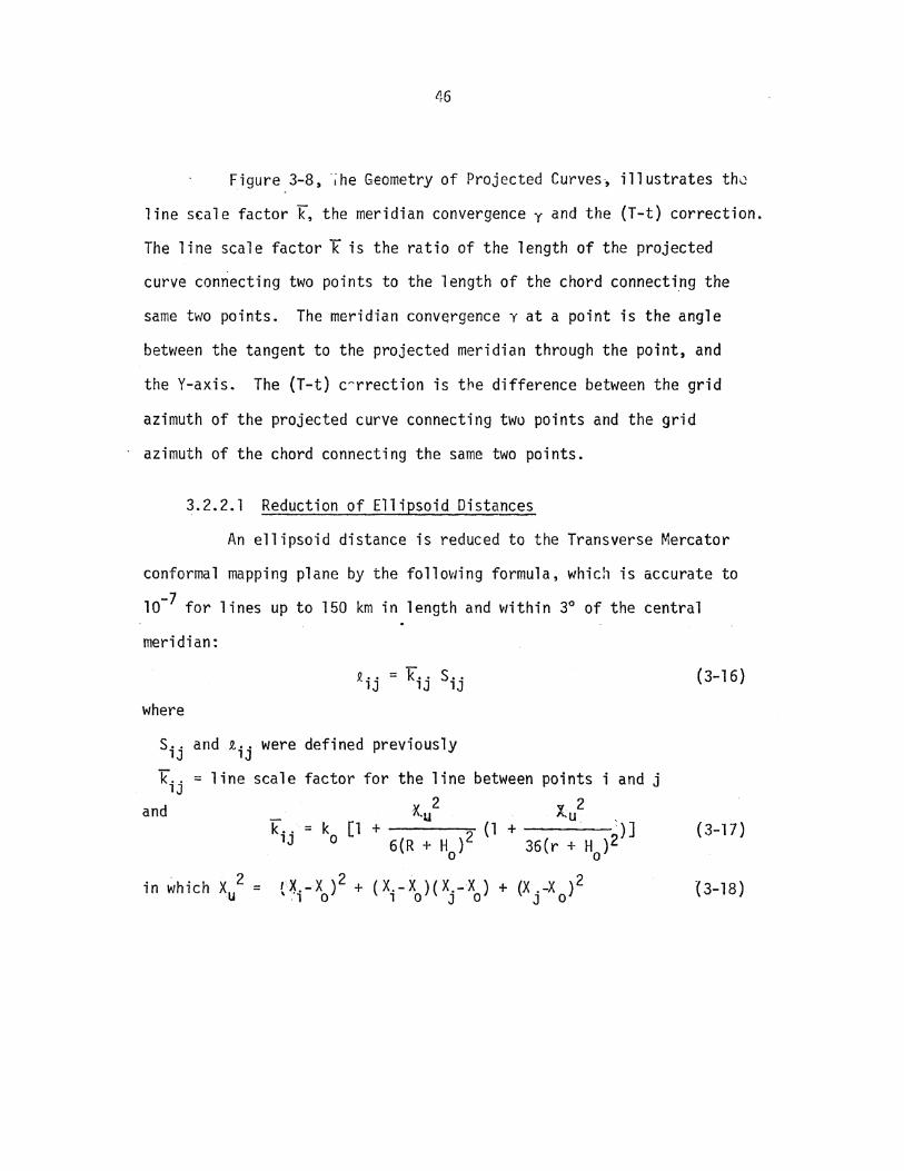
Figure 3-8, ·i he Geometry of Projected Curves·, i 11 ustrates th~
line scale factor k, the meridian convergence y and the (T-t) correction.
The line scale factor k is the ratio of the length of the projected
curve connecting two points to the length of the chord connecting the
same two points. The meridian convergence y at a point is the angle
between the tangent to the projected meridian through the point, and
the Y-axis. The (T-t) c~rrection is tre difference between the grid
azimuth of the projected curve connecting two points and the grid
azimuth of the chord connecting the same two points.
3.2.2.1 Reduction of Ellipsoid Distances
An ellipsoid distance is reduced to the Transverse Mercator
conformal mapping plane by the follovJing formula, which is accurate to
10-7 for lines up to 150 km in length and vtithin 3° of the central
meridian:
where
£ •• = k .. s .. lJ lJ lJ
s .. lJ
and tij were defined previously
k .. = lJ
line scale factor for the line between points i and j
and - x.,/ x./ k .. = k [1 + 2 (1 + :)] lJ 0 6(R + H ) 36(r + H )2
0 0
in which X 2 = {X.-X )2 + ( X.-X )( X.-X ) + ·U :·1 0 1 0 J 0
(X .-X )2 J 0
(3-16)
(3-17)
{3-18)

y
i .
47
projected meridian
to projected meridian
~projected curve
~ · -tangent to S projected geodesic
p raj ected para 11 e 1
~----------------------------------------------~~x
X, Y = grid coordinates S = length of projected curve d = c;JOrd 1ength k = line scale factor a = geodetic azimuth y = meridian convergence T = grid azimuth of projected curve t = grid azimuth of chord
Figure 3-8
Geometry of Projected Curves

48
3:2.2.2 Reduction of Geodetic Azimuths
A geodetic azimuth is reduced to the conformal mapping plane
by the following formula:
t. ·=a .. - y· - {T-t) .. 1J 1J 1 1J
where
a .. was defined p\·eviously 1J
yi = meridian convergence at point i
{T-t)ij = the {T-t) correction between points i and j
(3-19)
~1eri dian convergence for the Transverse Mercator projection
is given by the following expression \'lhich is accurate to o~·o1 within
3° of the central meridian: 2 2 8A· cos $· 2 4
~ . :: 8A . sin cp • [1 + 1 1 { 1 + 3n . + 2n . ) 1 1 1 3 (p 11) 2 1 1
4 4 8Ai cos $; + {3-20)
where
8Ai = change in longitude from the central meridian; positive east and
negative west to conform to the usual sign convention for
longitude
and 2 2f - f 2 2 ni = cos cpi {1 - f) 2
{ 3-21)
The (T-t) correction for the Transverse Mercator projection
is given by the follm-Jing expression \'-lhich is accurate to 0~02 for
lines up to 100 km in length within 3° of the central meridian:

49
(Y.-Y.) (X.+2X.-2X) (T -t) . . = J ~ J 1 o
lJ 6(R+H )2 0
(Y .+2X. -2X. )2 [1 - J 1 0 ] p"
27 {R+H )2 0
(3-22)
where all the terms have been defined previously.
For purposes of determining approximate grid coordinates.
tij ~ Aij ~ ~A; sin$; (3-23)
where all the terms havP. been defined previously. This approximate
reduction formula considers only the approximate meridian convrrgence
which is generally much larger than the other corrections included
in the complete reduction formula.
3.2.2.3 Reduction of Horizontal Directions
A horizontal direction is reduced from the ~llipsoid to the
Transverse Mercator conformal mapping plane by the following formula:
d .. P =d .. e- (T-t) .. 1J 1J 1J
(3-24)
where
d .. P = horizontal direction on the mapping plane from point i to 1J
point j
dij e and (T-t)ij were defined pre,yiously_.
3.2.2.4 Reduction of Horizontal Angles
A horizontal angle is reduced from the ellipsoid to the
Transverse Mercator conformal mapping plane by the following formula:
p e ( 8··k = S· 'k + T-t) .. - (T-t).k lJ lJ lJ 1
(3-25)

50
where
sijkp = horizontal angle on the mapping plane at point i from points
· j to k
Sijkt was defined previously
(T-t) was defined previously except that now one (T-t) term refers
to line ij ari the other to line ik
3.2.2.5. ~ag~itud~ Of the Corrections
Figures 3-9 to 3-11 inclusive show the magnitude of corrections
to observations in reducing from the ellipsoid to the Transverse
Mercator conformal mapping plane.
Figure 3-9 shows the scale factor correction for the 7ransverse
Mercator projection. The correction is proportional to the length of
the line and increases approximately as the square of the distance of . the line from the central meridian. At 10 km from the cent~al meridian
the correction is about 2ppm, at 50 km about 44ppm · and at 100 km about
175ppm. Neglecting this correction in horizontal position computations
on a plane would obviously only be possible in a very small area.
Figure 3-10 shows the meridian
convergence correction for the Transverse Mercator projection. Like
the slope correction to a spatial distance, this correction is so large
that it i~ applied even.in the lowest order horizontal position
computations.~ __
Figure 3-11 shows the (T-t) correction for the Transverse
Mercator projection. This correction is larger than 111 only for very
long lines having large north- south components.

........ ,...... II
0 ~
1. 0002
s.... 0 +l u <a u..
1. 0001
CLI ,...... <a u Vl
\
51
Conditions
S .. = 5 km lJ
¢ = 45° m
H = 0 o m
Distance of Midpoint of Line from Central Meridian (km)
Figure 3-9
Scale Factor Correction (Transverse f~ercator Projection)
-La
I ......... E
c: 0
·-0.3 •r-
I +> u CLI s.... s.... 0 u

52
5000" 1 (1°23'20")
/ Cor.ditions I I
¢. =- 45° I 1
2500" 1 (0°41 1 40") I
Central f1eridian (km)
-100 50 100
-2500"
-5000"
Correction (seconds)
Figure 3-10
t4eridian Convergence Correction (Transverse t4ercator Projection)

53
I
6.0 t 4.0
. 2. 0
I -,
-~.0 -
-4.0 . -·
-6.0
Correction (seconds)
Figure 3-11
v.-v: =so km J 1
the Central lleridian (km) -~·
100 50
\ v.-Y. =.:.so km
J 1
(T-t) Correction (Transverse ~1ercator Projection)

4. DETERMINATION OF DEFLECTIONS OF THE VERTICAL
In this chapter various methods of determining deflections of
the vertical i~ the small area covered by an engineering survey will
be considered. Unless noted otherwise, all deflections will be surface
deflections rather than geoid deflections since it is the surface
deflections that are required to make the gravimetric corrections to
the traditional survey observations.
A chapter is devoted to this topic because of all the
corrections applied to the traditional survey observations only the
gravimetric correction to horizontal position observations, being a
function of deflection of the vertical, is difficult to determine. All
other corrections are functions of the observations themselves, the
approximate positions of the ends of the lines of observation, or
quantities ~uch as the radius of the reference ellipsoid (R + H0 ),
reference gravity G, etc.; all of which are readily available. These
corrections can therefore be easily made if the accuracy of the survey
requires it. The. gravimetric corrections on the other hand are often
neglected for no better reason than the fact that deflections of the
vertical are difficult to determine. Section 4.2 describing a new
simple method to determine deflection of the vertical will show that
this no longer has to be the case.
54

55
Parameters describing the earth•s gravity field, one of
which is deflection of the vertical, are most often used to determine
the general shape of the geoid over a large area. Fo~ purposes of
national geodetic control this is sufficient. However, for purpos~s
of local geodetic control, for example engineering surveys requiring
high accuracy, local variations in the earth•s gravity field may have
to be considered. For this reason, in this chapter only methods
having a resolution sufficient to determine a change in deflection of
the vertical in the order of 211 in 5 km will be considered.
In the following sections seven methods to determine deflection
of the vertical, which meet the resolution criteria, will be discussed.
The existing methods will be discussed only briefly. The astrogeodetic
difference method wiil be discussed in detail, and field test results
from the trigonometric method and the astrogeodetic difference method
will be presented and evaluated.
4.1 Review of Existing Methods
4.1.1 Trigonometric Method
This method through which change in deflection of the vertical
is determined is well known, but it is·seldom used because the uncer
tainty associated with vertical refraction makes it difficult to deter
mine the accuracy of the result. Only in mountainous areas where
atmospheric conditions are stable and lines of observation are high
above the ground does the method appear to give satisfactory results
[Hradilek, 1968].
56
V.Jher. trigonometric levelling is used to determine change in
deflection it is usually done within a three-dimensional adjustment in
which c:, and n of each point are solved for as unknown parameters
together with thr. three-dimensional roordinates of each point. The
use of trigonometric levelling_data in a three-dimensional adjustment
is in fact the only new development associated with this method ~ince
problems with the method were outlined by Kobold [1956].
A unique solution f0r change in deflection of the vertical
along the line connecting_ two points can be made if accurate trigonometric
and spirit levelled heigpt differences are available and if the
coefficient of refraction is assumed to be the same at each end of the
line.
From simultaneous reciprocal trigonometric levelling
[Chrzanowski, 1978], z -z ~hAB = Ss sin ~
where
~hAB = difference in trigono~tric height between points A and B
Ss = slope distance between points A and 8
zA,zB = simultaneous reciprocal zenith angles at points A and B
corrected for defiections of the vertical.
(4-1)
If ~HAB is the spirit levelled height difference between points .A and z -z
8, then(Ss si.n ~- ~HAB) is the separation, at point B. of the
reference ellipsoid passing through point A and th~ equipotential surface
passing .through point A.
This separation is related to the change in deflection of the
vertical along the line between the two points by.[Vanicek and Krakiwsky.
in prep]
57
2LlN !J.£ = -~
where
tJ.c. = change in deflection of the vertical
t:.N = difference in ellipsoid - equipoteAtial surface separation
S0 = ellipsoid distance between the points.
Substituting for N, and expressing ~c.-ln seconds, 2(t~H - S sin -8-·~ ) AB s 2
so • - ---------- pll "c.AB .- ·
(4-2)
(4-3)
where tJ.c. positive means that the change in deflection of the vertical
is outward along the line joining the points. To determine tJ.c.AB from
this formula iteration is required because llc.AB.appears on both sides
of the equation: explicitly on the left hand side, and as a correction
to observed zenith angles on the right hand side.
f,s was noted previously,. when the difference in trigonometric
and spirit levelled height differences is assumed to be due nnly to a
change in the deflection it is necessary to assume that the coefficient
or refraction is the same at each end of the line of observation. The
coefficient of refraction kin this case is [Chrzanowski, 1978].
_R_ [180° - (zA + z8}] + 1 s pll
0
where zA' zs-• S 0 and p 11 were defined previously and
R = mean radius of the reference ellipsoid.
(4-4)
A completely different approach can be taken in which the
difference in trigonometric and spirit levelled heights is assumed to
be due to only a difference in coefficient of refraction at each end
of the line of observation. The necessary assumption now is that there
is no change in deflection from one point to another. The coefficient
of refraction from point A to point B, kAB' in this case
is [Brunner, 1977]
( 4-5). S s . 2 s s1n zAB
A simil~r expression can be written for the coefficient of refraction
from point B to point A, k8A.
4.1.2. Astrogeodetic Method
This method was mentioned previously in the context of
establishment of a horizontal geodetic datum. (See section 2.2.1~)
The formula for the components of the deflection of the
vertical are
\'lhere
r; = q, - ~
n = (A - A) cos ~
(4-6)
(4-7)
{r;, n) =components of deflection of the vertical, north-south
and east-west respectively
(q,, A) = astronomic coordinates, latitude and longitude respectively
(~, A) = geodetic coordinates, latitude and longitude respectively.
This i~ the classical method of determining deflection of
the vertical, and should provide the highest accuracy. (See Section
4.3.2.) The only disadvantage of this method is that laborious and
costly 2nd order astronomic observations are required.
4.1.3 Gravimetric Method
This method uses gravity anomalies to determine deflections
of the vertical. The conversion of gravity anomalies to.def~ection of
the vertical is by the well knovm Vening-fcleinesz formulae:
where
{cpA, A.ti) = point of interest
(cp, A) = running or dummy point
59
dv (4-8)
G =mean value of gravity on the surface of the refere~ce ellipsoid
= 9.8 m;s 2
Ag = gravity anomaly.
a= geodetic azimuth between (cpA' AA) and (cp, A)
d ~$1/1) = Vening-f1einesz funtion; a known function of spherical distance
v = solid angle between (cpA, AA) and {cp, A)
Often gravimetric deflections are only used to interpolate deflections
between points at which astrogeodetic deflections have been determined.
This approach is knm'in as the astrogravimetric method.
Deflections from gravity anomalies are deflections at the geoid
with respect to a geocentric reference ellipsoid. Small corrections
would have to be made for curvature of the p1umbline (the difference
between geoid and surface deflection- see section 2.2.1), the datum
shift and what is known as the indirect effect (see Vanicek·and
Krakiwsky [in prep]) to obtain surface d~flections with respect to a
nongeocentric reference ellipsoid. In addition to this, the theoretical
requirement of the Venin~-Meinesz formulae is that Ag must be given
continuously over the entire earth. However, because the gravfmett"ic

60
deflection is often us~d only for interpolation, the Vening-f·1einesz integration
can be carried out over a small area (say 100 km radius) in the region
of intere~t to obtain incomplete gravimetric deflections. These
;~complete gravimetrir. deflections {which are also uncorrected for
curvature of the plumbline, datum shift and the indirect effect)
differ from the correct ones by an almost constanc amount and thus are
adequate to obtain accurate interpolated values of deflection between
points of know~ astrogeodetic deflection •
The interpolation between points of known astrogeodetic
deflectioncan be linear U1olodenskii, et al , 1962] but this results
in a loss of information since deflections are inherently two dimensional.
The loss of information is overcome by a method developed at the
University of New Brunswick [Merry, 1975] which uses a two dimensional
surface to interpolate between points of known astrogeodetic deflection.
One disadvantagE' of the ~ravimetr'ic or .astrogravimetric methods is that
large amount of gravity data is required. A second disadvantage is the
computational complexity of the method. Access to a large computer
would be essential if these methods were to be used.
· 4.1.4 ·Topographic Method
Deflections, at a local level, are highly correlated with
topograpny; as a result variations in deflections in rugged terrain are
due almost entirely to the topography.
The formulae for the deflection components in a rectangular
coordinate system expressed as a function of adjacent masses is given
by_ Fischer [1974]:

61
(4-9}
wliere
K = universal gravitational constant = 6.81 x 10⁻¹¹. m3kg-ls-2
G = mean value of gravity on the surface of the earth= 9.8 m/s2
m = mass of an adjac{'nt unit of mass
(Ym-YA), (Xm-XA} = horizontal distance f1om the centroid of the
unit of mass to the point of interest.
Numerical integration of the formulae is required but it can
be readily seen that the effect of distant masses decreases rapidly
because of the s3 term in the denominator. When used to determine
deflections on an atoll in the Pacific Ocean [Fischer, 1974] an
integration distance of several hundred kilometers proved to be
adequate. The assumption of a flat earth, implicit in the formulae,
was also adequate. ·If topographic deflections were used to interpolate
between known astrogeodetic deflections, in the same way that incomplete
gravimetric deflections are used in the astrogravimetric method, a
much shorter integration distance would be satisfactory.
The se~ious disadvantage of this method is that the density
distribution of the earth in the vicinity of the point of interest should
be known. In very rugged terrain however, where the topography itself
rather than the density distribution within the topography has the
predominant effect, the method produces accurate results. On the Pacific
atoll referred to previously a standard deviation of the difference in
deflection (between astrogeodetic deflections and topographic deflections
based on a simple density distribution model) of 1~5 \'Jas obtained for

+Y
6?.
23 deflections ranging from about -30 11 to +30 11 • In the horizontal
control network for the 20 km long Simplon tunnel in Switzerland
deflections were calculated by this method usin~ only the visible
mountain masses. (Richardus, 1974].
As an illustration of the general effect of topography on
deflection consider the follovling example. Figure 4-1 shows hills
having slopes nf 5%, 10%, 50% and 100%; all 2 km long at the base.
/
/ / 100.%
25~'6
10% 5%
~------ -----·----;;.->-~1<<--------km 1 km
Figure 4-1 General Effect of Topography on
Deflection of the Vertical
~ ---·--==-··---~
63
The hills are also 2 km l:Jng in the plane of the page and have the
same cross section from one end to the other. The material in the
hills has a uniform dP.ns1ty of 2670 kg/m3• The deflection of a point
half way up to the north side of each hill with respect to zero
deflection at a point not on the hill or a point at the top of the
hills is 1~'5 for th~ hill of 5% slope, 3~0 for-the hill of 10% slope,
14~4 for the hill of 50% slope and 25~6 for the hill of lOG% slope.
All. deflections are "downhill".
4.1.5 Combined Method (Least Squares Collocation Method)
A method of this type combines heterogenous data through
least squares collocation to produce an optimal solution. By a
combined method it is possible to compensate certain disadvantages
in one type of data by advantages inherent in data of another type,
and to interpolate numerically between discrete observations
The method of Lachapelle [1975] which combines astrogeodetic
deflections, gravity anomalies and low degree geopotential coefficients
is a method of this type. The low degree geopotential coefficients
provide the general features of the geoid and define a reference
surface. The finer features are provided by astrogeodetic deflections
which are accurate but widely spaced, and gravity anomalies which are
usually abundant on land but sparse in the oceans. The solution for
deflection at any point is given on the geoid with respect to a
geocentric reference ellipsoid. The solution can be given with respect
to any nongeocentric reference ellipsoid if its datum shift parameters
are known. For a complete description of this method see Lachapelle [1975].

64
The disadvantages of this method are the same as those for
the astrogravimetric method, that is data and computational requireme·nts,
only more so.
4.1.6 Inertial Hethod
An inertial survey system {ISS) has two types of main sensors,
gyroscopes and accelerometers. The. gyroscopes maintain the alignment
of the ISS, and from the accelerometers a change. in positlijon can be
determined by double integration of acceleration over time. This is
the basic concept on an ISS; an actual ISS. is a complex electromechanical
device with many error sources. Adams [1979] describes the lor.al
level ISS and simulates position errors of.the system caused by
accelerometer bias and gyro drift.
The primary use of an ISS has been to determine horizontal
posi.tions between 2nd order points; Because of the sensors in an ISS,
changes in deflection of the vertical can also be measured. Figure 4-2
show~ the basic concept. In this figure, E is the deflection, g is the
gravity vector andy is the vector normal to the_ reference ellipsoid. Accuracies ..
of the order of 2" have been reported [Tod~ .. 19.78] but there are apparently
systematic errors due to the filtering procedure [Schw~rz, 1978].
ISS's are very complex and barely beyond the prototype stage
but the speed and ease with which changes in deflection can be determined
may offer advantages in certain applications. The method, if not

65
equipotential surface
_i - -:_-;-::::::::::.::..:::::::::_=-.::: __ \_ ------===:::::::==.
~~-- p
reference ellipsoid
Figure 4-2
Basic Ccncept of Heasurement of Change
in Deflection by an ISS
frame transported
2
already economically competitive with other methods to determine
changes in deflection, will certainly be so in the future as Iss•s
become more generally available.
4.2 Astrogeodetic Difference Method
4.2.1 Description
This method to determine change in deflection of the vertical
has been developed by the author, and to his best knowledge, it has
never before been used.

66
The method i~ based on relative rather than absolute astroncmic
observatio1s; that is it is a difference method. Accuracies of the
order of 1" appear to be attainable using two 1" Theodolites with
automatic vertical circle compensators and two-way radio communication
so that a timer can give a simultaneous read signal to both observers.
The reason that the high accuracy is attainable is that, as with other
difference methods, a difference of tvJO observabl es can be measured more
accurately than either observable itself. by differencing, the effect
of common systematic errors is eliminated.
~ = ~ - ~ and n = (A - A.) cos ~ are the expressions for the
meridian or north-south,and prime vertical or east-west deflections of
the vertical respectively, where (~. A) are astronomic latitude and
longitude and ($,A.) are geodetic latitude and longitude. After differ-
entiation, the expressions become
and
d~ = diP - dcj>
dn = ·(dA - dA.) cos cp
~ (dA - dA.) cos 4>
(4-10)
(A - A.) sin ~ dcp ( 4-11)
For sma 11 changes in t; and n,d' can be replaced by ¢. • It would also
be permissible to. drop the term {A-A.) sin cpll.<f> for determinations of
ll.n in which.ll.cp were small. . . .
For example, with {A -.A) = ao", <j>=45°,
llcp = 1000" (32 kn!:!:_), the error in neglecting the second term \</Ould be only +0~'1.
To determine ~he differences llcp and ll.A. various. methods can be used. Fo1
ll.<f> and ll.A. to be accurate to 0~1, ll.Y and ll.X have only to be accurate to
about 3 m and 2 m respectively at 4> = 45°. ll.<f> and ll.A. can therefore
be determined from a large scale map, if it is available, or from any
horizontal position determination--giving a relative positional accuracy
of about 2 m.
67
A~ and AA in the math models for A~ and An are determined
by simultaneous astronomic zenith angles.
·By applying spherical trigonometry to the astronomic triangle,
or equivalently, by transforming between the horizon. and hour angle
celestial coordinate systems through the use of rotation matrices the
following expression can be obtained [~1ueller, 1969]:
cos i = sin 8 sin ~ + cos 8 tJS h cos ~
where
z = zenith angle to the star
6 =declination of the star as tabulated by a star catalogue
~ = astronomic latitude of the point of observation
h = hour angle of the star
(4-1!)
After differentiation with respect to the observed quantities
~ ~ and·h, and simplification (see Appendix I), the expression becomes
~~ = - sec A AZ - cos ~ tan A Ah ( 4-13)
This expression is used in Mueller [1969] to show the effect of small
systemmatic errors in the measurements of zenith angle and hour angle
on the determination of astronomic latitude. When the expression is
used to determine M between two points at which simultaneous
observations of zenith angle of the same star are made, then
A~ = - sec A Az since Ah = 0. Further, if the star is chosen such
that A - 0, then M = - A z.
The ideal choice of a star for the determination of A~ in
the Northern hemisphere is obviously Polaris (a Ursae Minoris) since

68
its azimuth at any time is very small. To illustrate this, consider
the choice of Polaris for the determination of~~ at~= 45°. The
azimuth of a star is maximum at elongation, and [Mueller, 1969]
. -1 ( ) Aelongation = s1n cos o sc~ ~ . ( l- 14)
For Polaris ,
0 = 89° 10 1 (1979), and
Ael ongation = .:!:_ 1 ~2, sec A = 1. 0002
Thtrefore, if.Polaris is chosen for the determination of ~~at
~ = 45°, the math model ~~ =- ~z can be used in place of~~= 'sec A ~z
with a maximum error of -0~2 in 1000. 11
In order to determine ~A from simultaneous astronomic zenith
angles, the expression for zenith angle, cos z = sin o sin ~ + cos o
cos h cos ~, is again used except that astronomic longitude A is
entered into the expression by making th~ substitution
h=A-a.+T
where
h and A were defined previously
a. = right ascension of the star as tabulated by a star catalogue
T = time
(4-15)
After differentiation with respect to the observed quantities
z, ~.A and T, and simplification (see Appendix I), the expression
becomes
~A= - sec ~cot A~~- sec~ cosec A ~z- ~T (4-16)

69
This expression is used in r~ueller [1969] to show _the effect of small
systematic errors in the measurements of astronomic latitude, zenith
angle and time on the determination of astronomic longitude. When
the exr-ression is used to determine AA beb1een two points at '.-hich
simultaneous observations of zenith angle of the same star are made,
then bA= - sec 1 cot A bl - sec 1 cosec A bZ since bT = 0.
The appropriate choice of a star for the determination of
~A is one for which A=~ 90°, that is a star near east or west prime
vertical crossing, since with A=~ 90°, cot A= 0, cosec A~ 1 and
~A = - sec ~ ~z. The last expression shows only the predominant term
in the determination of ~A; to avoid large errors the complete expression
must be used in which ~~ was determinsd previously, ~ is the tpproximate
astronomic latitude and [Mueller, 1969]
A _ -1 (sin o - cos z s -; n tP - cos sin ~ cos 1
where
o and 1 were defined previously
: zl + ':Z z = 2 2 + refraction correction
) ( 4-17}
In the actual determination of AA, the star chosen is one
near -~ast or 'West prime vertical crossing at the time of observation.
To positively identify the star, the approximate azimuth, zenith ans1e
and time are used to compute the approximate declination o and right
ascension a of the star. From [Mueller, 1969]
70
6 = sin-1 (cos A sin ~ cos 1 + cos t sin 1) (4-18)
a = A _ h + UT + R; h·= cos-1 (cosz - sin o -sin 1) cos o COS I
where (4-19)
a, A, z, 1, a, A, and h were defined previously
UT = universal time
R = a - 12h m in which am = right ascension of the mean sun.
R or am are tabulated in star catalogues. With the star identified,
the tabulated value of o is used in the formula for azimuth.
The description of the determination of ~~ and 8A is complete
except for the application of the differential refraction correction.
In order to make this correction pressure and temperature are measured
at both points before and after each set of observations. The
differential refraction correction is then applied to ~z by using
refraction tables, for example those provided in Mueller [1969].
Summarizing the method of determining change in deflection of
the vertical by the astrogeodetic difference method;
(4-10 repeated)
where
·~~is determined approximately {to 0~1) by any suitable method,
~~ (for Polaris)=- ~z + diff. refr. carr.; (4-20)

71
An = (AA - 41) cos ~ ( 4-11 repeated)
where
AA. is d·etermined approximately (to 0~1) by any suitable method,
M = - sec ct> cot A M - sec ct> cosec A (t.Z + diff. refr. corr.), (4-21)
in which M was determined previously a11d A is calculated
from z, ct>, and 6 of the kncwn star near prime vertical
crossing.
An HP-29C program for the determination of M from 8.":!, is
given in Appendix II.
4.2.2 A Priori Error Analysis
Applying the law of propagation of errors to the math model
for M,, 2 - 2 + 2
a A~ - a A~ a A~ (4-22)
If the error in M is assumed· to be-small in comparison to the error
in -M , therr - . - - 2 2 a A~ = a Act> (4-23)
Applying the law of propagation of errors to A~ = - A~ + differential
refraction correction, 2 = a2 . + 2
a M AZ cr Ar (4-24)
where
A r = differential reftaction correction
and 2 . 2 + ~2 . a A~ = a AZ v Ar (4-25)
In the measurement of zenith angles there are three errors;
the error in reading the zenith ang1e in the readout system, the error
in pointing the vertical crosshairs of the instrument at the target
and the error in levelling of the vertical circle index.
72
The reading, pointing and levelling errors (crr' crp and cr1
respectively) are determined by the types of instruments used to make
the simultaneous zenith angle measurements. For example, if two -
28X, 111 theodolites with automatic vertical circle compensators and
artificial light for the readout system were useQ, the errors would
be:
cr = 111 (from previous experience of the author) r
cr = 0~5 (from Chrzanowski [1977]) p
cr = 0~3 (from Cooper [1971]) 1
The error in the differential refraction correction {crAr)
is estimated to be of the same order as the correction itself, and
a value of 0~5 is u~ed.
For each determination of Az, four measurements of zenith
angle are taken (one measurement on each face of each instrument}.
If the previous vaiues of crr, crp' a1 and cr6r are used, the standard
deviation for each determination of A~ would be
2 2 1/2 0 6~ = (cr Az + 0 A r) · '
( 2 + 2 + 2) 2 112 = [4 crr crp o1 + cr6r ]
= 2~1 4
crr, op' cr1 but not crAr can be reduced by ;n sets, therefore
if, for example, 12 sets are taken

73
[ 4 (12 + ~.52 + 0.32) + 0.52}1/2 = 0~8 12
Applying the la1-1 of propagation of errors to the math model
for ln1,
2 2 2 + 2 ~ 2 cr &n = cos cp cr &A cos ~ cr &A (4-26)
If the error in ~A is assumed to be small in comparison to the error
in M, then 2 2 2
J &n=COS t/> a M (4-271.
Assuming that &A is determined when the star is near prime vertical
crossing,
&A ~ sec ~ ( &z + &r)
Applying the law of propagation of errors to this expression,
2 - 2 .( 2 + 2 ) cr AA - sec ~ a &z cr &r
Substituting into the expression abJve fo·~ o 26n ..
cr2 = 2 + r/ lln cr Az llr
which is the same as the expression for cr 2ll~·
(4-28)
(4-29)
(4-30)
In the determination of Az for An however, there is a simultan-
eous timing error in addition to the other errors. This error is
negligible in the determination of A~ because for ll~ a star near the
celestial pole is observed. The apparent motion of this star is vet·y
slow. For.AA a star near prime vertical crossing is chosen. The
apparent motion of a star, along its track, at prime vertical crossing
equals the rotation rate of the earth, that is 360° per 24 hours or

74
15" arc per ls time, making the star more difficult to track and to
point to at an instant of time. The vertical component of the apparent
motion of~ star at prime vertical crossing is 15" cos cp per ls.
Thr simultaneous timinr error {aAt) of two observers reacting to a
read signal given by a third person is estimated to be 0~1. At
cp = 45° this corresponds to an error in zenith angle of 1~0. If the
previous values of ar• ap,a~ and aAt are used, the total standard
deviation for each determination of An is
a An = 2 2 l/2
(aAz + aAr )
[4 ( 2 + 2 + 2 + 2) 2 l/2
= ar ap a~ aAt + a Ar ]
l/2 = [4 (1 2 + 0.52 + 0.32 + 1.02) + 0.52]
= 31:1
ar' ap' a2 ~ aAt but not aAr can be reduced by In sets,
therefore if,for example, 12 sP.ts are taken
aAn = [4(12 + 0.52 ;20.32 + 1.02) + 0.52]1/2 = 1~0
This error analysis for A~ and An assumes that there is no
systematic shift between the two observers and instruments making the
simultaneous observations. To check for this possibility, a set of
simultaneous zenith angles on the same star near prime vertical crossing
should be determined faY' the two observers and instruments side- by side.
This procedure should be performed at the beginning and at the end of
a night of observations.

75
In the field work which was done {see section 4.3) some
practice time was required to eliminate this shift. It was noticed
during these practice sessions that shifts as high as 10" could occur
when one or more of the following condition~ existed:
1. parallax betv-1een the instrument crosshairs and the star~
2. vibration of the vertical circle compensator causing vibration
in the readout system because of an unstable instrument setup,
3. ~oar lighting of the crosshairs and readout system.
During the observations care must be taken to eliminate these conditions:
crosshairs and star must be properly focussed, a stable instrument setup
must be made and batteries for the lighting system must be changed as
soon as the light begins to dim.
4.3 Field Tests
In order to determine whether the astrogeodeti c difference
method was actually practical and produced results more or less consistent
with other independent determinations, field tests were carried out in
the Fredericton and Fundy Park areas.
In the Fredericton area results from the astrogeodetic
difference method were compared with results from the trigonometric
. method and results provided by Dr. Lachapelle using his combined method.
Dr. Lachapelle also provided results for the Fundy Park area and these
were compared vii th results from the astrogeodeti c method and the astro
geodet·ic difference method.

76
The astrogeodetic difference and trigonometric methods
produce surface deflections of the vertical. The results which Dr.
Lachapelle provided are geoid deflections. Section 2.2.1 gives the
maximum curvature of the plumbline between the geoid and the terrain as
311 /1000 m height above the terrain; therefore for both the Fredericton
area (H ~ 10 m) and Fundy Park area (H ~ 350m) the geoid deflectiQnS
provided by Dr. Lachape 11 e are essenti a·lly the same as the surface
deflections.
Dr. Lachapelle's results were determined from the Goddard
Earth Model (GEM) lOB potential coefficients and adjacent gravity
anomalies. No astrogeodetic deflection data was used in either the
Fredericton or Fundy Park areas.
4.3.1 Fredericton Area
J:igu.re 4-3 shows the location of three points in the Fredericton
area ("Pillar 11 , "~1aple 11 and "Minto") between which changes ir. deflection
of the verti ca 1 were determined.
The Fredericton area was chosen for convenience and, in order
to utilize the terrain to make the changes in deflection as large as
possible, the three points were located on opposite sides of the St. John
and Nashwaak River valleys. "Pillar" is the East astro pillar located
on the roof of the Eng·: neeri ng Building, University of New Brunswick ..
11 Maple" is marked by an orang~· colored ,wooden stake on a slight rise in
an open field. "Minto" is marked by a brass marker set in a rock outcrop.
The line between 11 Pillar" and 11 Minto" is denoted as line 1, the line

-....,J -....,J
Scale 1:25 000 All elevations in feet
r 0 2 4 6 8 10
Scale for Deflections {seconds)
Figure 4-3
Deflections of the Vertical in the Fredericton Area
by the Astrogeodetic Difference Method

78
between 11 Pillar11 and 11 Maple 11 as line 2 and the line between 11 Maple"
and "lvlinto11 as line 3.
4.3. 1.1 Use of the Trigonometric Method
The trigonometric method was used only on line 1.
The slope distance (Ss) of line 1 was measured independently
by four groups of students using microwave EDM equipment, and is
believed to be accurate to+ 0.1 m.
The difference in heigf)t (..~H) between "Pillar 11 and 11Minto 11
{each end of line 1) was measured by two groups of students under the
supervision of the writer. Precise levelling equipment was used and
precise levelling procedures were rigorously followed. The levelling
route was divided into short sections so that blunders.could be
isolated. The misclosure in each section and for the entire levelling
route was smaller than that required for special order levelling which
has an allowable misclosure of~ 3 mmjlkm of levelling route [Surveys
and Mapping Branch (EMR), 1973]. The total misclosure for the entire
route was 0.00527 m. Based on 200 sightings and a standard deviation
of 0.4 mm/sighting [Chrzanowski, 1978], the standard devaition of the
height difference was estimated to be ~ 0.006 m. Because the forward
and backward levellings were performed on essentially the same route,.
the gravity correction was negligible.
The standard deviations given for 6E, k, kAB and kBA were
determined by applying the law of propagation of errors to the expressions
for each of these terms. In each case, the contribution of the standard

79
deviation of 4H , Ss and S0 was negligible in ca.mparison to the contri- ·
bution to the standard deviation of z:
( 4-31 ).
(4-32)
2 R 2 2 2 cr = (-s u) (cr ·z + <1z ) k oP A 'B
(4-33)
where
cr 2 = {standard deviation )2 or variance
The standa~~ deviation of each zenith angle was determined from a set
of 12 zenith angles. Each. reciprocal zenith angle was measured
simultaneously {by means of two-way radio communication)and in rapid
succession.
Line l is far from an ideal choice of a line on which to
determine an accurate trigonometric height difference. According
to Bamford [1975] there are several unfavorable situations·for the
determination of accurate trigonometric height differences:
1. great width of river crossing,
2. low ground or water clearance,
3. asyrrunetry of terrain profile,
4. aymmmetry of ground and water,
5. clear skies,
6. great heat or cold,
7. absense of wind.
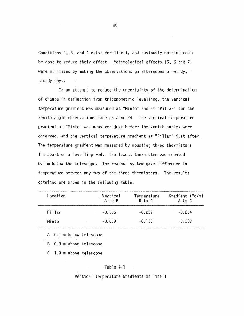
80
Conditions 1, 3, and 4 exist for line 1, anJ obviously nothing could
be done to reduce their effect. Meterological effects (5, 6 and 7)
were minimized by making the observations gn afternoons of windy,
cloudy days.
In an attempt to reduce the uncertainty of the determination
of change in deflection from trigonometric levelling, the vertical
temperature gradient was measured at "Minto 11 .and at "Pillar11 for the
zenith angle observations made on June 24. The vertical te~perature
gradient at "Minto" was measured just before the zenith angles were
observed, and the ver.tical temperature gradient at 11 Pillar" just after.
The temperature gradient was measured by mounting three thermisters
I m apart on a levelling rod. The lowest thermister was mounted
0. l m below the telescope. The readout system gave difference in
temperature between any two of the three thermisters. The results
obtained are shown in the following table.
Location
Pillar
Minto
A 0.1 m below telescope
Vertical A to B
-0.306
-0.639
B 0.9 m above telescope
C 1.9 m above telescope
Table 4-1
Temperature B to C
-0.222
-0.133
Vertical Temperature Gradients on line 1
Gradient ( 0 c/m) A to C
-0.264
-0.389

81
To min1mize the effect of heat from the Engineering Bu·ilding., zenith
angles and vertical temperature gradients for"Pillar'' were measured
close to the edge of the building.
The results were not what had been expected. If the average
value of vertical temperature gradient (A to C) is used to determine
coefficient of refraction,
from P dT k = 502 2 (0.0341 + dh) [Angus-Leppan, 1967] T
(4-34)
where
P = atmospheric pressure in millibars
T = temperature in °K
dT temperature gradient in °C/m dh = kPillar = -1. 37
k = -2 13 "Minto ·
An average value of vertical temper3ture ~radient of -0.009 °C/m had
been expected, which would have produced k values of about 0.150. The
conclusion that can be drawn is that vertical temperature gradients
in the immediate vicinity of the instrument are not representative of
the average vertical temperature gradient at one end of a line of
observation, probably because of the rapid change in ~~ and k near the
ground.·
A solution to this problem might have been to measure the
temperature gradient further away from the instrument but still along
the line of observation. For line 1 this was not feasible: at the

82
"Pillar" end the instrument was already near the edge of a high
building,.and at the "Minto" end the slope dropped off rapidly along
the 1ine of observation.
Table 4-2 shows the results of a difference in trigonometric
and spirit levelled height differences interpreted a~ a change in
deflection of the vertical (Approach 1) and as a difference in coefficient
of refraction at each erd of the line of observation (Approach 2).
For this particular line the difference in heights may have beln due . .
just as much to one as the other, but the relative contribution of
each could not be determined because of the unsuccessful attempt to
make an independent determination of the coefficient of refraction
at each end of the line of observation.
4.3. 1.2 Use of the Astrogeodetic Difference Method
The astrogeodetic difference method was used on lines 1, 2
and 3 so that the misclosure in ~~ and ~A could be calculat~d to
check for a possible systematic error in either of these quantities.
"Pillar" was arbitrarily assigned a zero deflection of the
vertical. The values of A~ and ~A were determined by measuring
azimuths accurate to about + 10" and EDM distances accurate to about
. 0.1 m, and applying Puissant's formula. Astronom~c coordinates
accurate to about 0~1 had been previously determined for "Pillar" and
these \'tere used in the computations, but approximate astronomic
coordinates would have been just as good.
In all the determinations of~~ and ~n , values f9r o, a, and

Observers Date Time Weather *\(m) *t.H(m) Approach 1 (Zenith Angle) M;(")
I I
,Lea 1 30% cloud 41.739 .:. 0. 0061 _,_ 4 .:. 1. 0 lc!IC ~lay 17 3:30 pm cover ,1 i ght 4833.0 + 0.1
ITeskey wind -I
!Lea 1 I 10n% cloud land May 20 112~30 pm cover,light 4833.8 + 0.1 41.732 ::t. 0.006! -ID.6.:t. 0.6 I
Tes~ey
I wind
Leal ,_
1 100% cloud jand June 24 4 pm r cover ,light 4832.5::!:. 0.1 41.695 + 0.006 -0.8.:. 0. 7 ITeskey wind
I
Appl'Oach 1: Samek at each end of the line of observation assumed.
Approach 2: No change in deflection of the vertical assumed.
k
0.136 + 0.005 -
0.139.:!: O.OG::i
0.147.:. 0.004
*Ss and ~H different for each set of observations bec~use ··nstrument and target setups different.
Table 4-2
Trigonometric Levelling on line 1
Approach 2 I kAB
. kBA !
i 0.163 + 0.011 o.1o3 + o.oc6 I - - j
I I I
I 0.150.:. 0.00510.128::!:. 0.004
0.162.:. 0.00710.131::!:. 0.004
I : o::> w
84
.. R for the stars observed were taken from 11 Ple Star Almanac for Land
Surveyors for the Year 197911 (SALS, 1979} [Her Majesty•s Nautical
Almanac Office, 1978]. 12 sets of observations were made. Values of
6~ and 6n were determined twice for line l to check that time of
observation and star observed did not have a significant effect.
The check for the systematic shift between the two observers
and instruments was performed before and after the observations for
6~ and 6n on line l. The check was performed only after the observa
tions for 6~ and 6n on line 2 because the results from line 1 had
shown no significant _systematic shift. (The system.atic shifts for
both determinations of A~ and 6n on line 1 were less than 111 and the
standard deviations were about 211 .) The check was not performed
after the observations for A~ and 6n on line 3 because no stars were
visible at the time due to heavy cloud cover.
One pair of.observers (Leal and Teskey) p.erformed the
observations on lines 1 and 2. A different pair of observers (Sujanani
and Teskey) performed the observations on line 3 •. This was done only
because Leal.was not available for the observati~ns on line 3.
Table 4-3 summarizes the determinations of 6~, AA, A~ and AA
in the Fredericton area. When M and M were not corrected for
differential refraction, the misclosures (about 111 for A~ and 2~·5 for AA)
were about the same magnitude as the standard deviations of the mis-
closures. When M and .AA \</ere corrected for differential refraction,
the misclosures (about 0~5 for A~ and 1~0 for AA) were about one-half
the magnitude of the standard deviations of the misclosures. These

Observers Date Line From To t~cp(ll) flA (II } M>(ll} M'(u) M(u) M(u) (uncorrected) (corrected) (uncorrected) (corrected)
Leal and June 27 2 Pi 11 ar Maple 97.2 15.2 94.9 .:t. l. 1 94.4 + l. 1 17.3 + 1.5 16.6 + 1.5 Teskey
Sujanani co and July. 7 3 Maple Minto -85.9 208.5 -80.9 + 0. 8 -80.4 + 0.8. 205.6 + 2.1 205.5 .:t. 2.1 U"1
Teskey & 8 - -
leal fay 22} {-13.0 + 0.8} rl3.3 .:t. 0.81t220.8 .:t_l.9lt221.5 .:t. 1.9~ and 23 1 Minto Pillar -11.3 -224· 7 -13.1 ~ 0.7 Teskey May1 ~7,
-13.5 .:t. 0.7 -220.3 .:t. 1.3 -221.3 .:t. 1.3,
Sum 0.0 0.0 D·o::1.6} {0.7:: l.j i2.1 :: 3.J (0.6 + 3.21 0.9 + 1.5 a. 4 + 1. 2.5 + 2.9 (o.9 ~ 2!9]
Table 4-3
Differences in Astronomic and Geodetic Coordinates in the Fredericton Area

86
results indicate that a small systematic error may exist in the results
and that the differential refraction correction may reduce the system
atic error. Table 4-3 also shows that the time o~ observation and
the star observed probably do not have a significant effect on the
determination of M and tJ.A since the two detenninations of M and
~A on line 1 are the same at the lcr level.
The final results, t; and n of "Maple 11• and 11 ~1into 11 with respect
to 1;_ = n = 0 at the pillar, are shown on Figure 4-3. The standard
deviations of the results compare well with those calculated from
an a priori error analysis. The t; and n values for "Maple" are those
determined from the astronomic observations at "Pillar11 and "Maple .. ,
and the t; and n va 1 ues for ur~i nto 11 are those dete.rmi ned from the
astronomic observations at 11 Pillar11 and 11Minto", that is neither
set of deflection components were adjusted for the small misclosure
around the triangl~.
Figure 4-3 also shows the deflection of the vertical as a
vector. When shown this way it appears that.the deflection is affected
by the topography in the general area of the station. This may be
by chance considering the magnitude of the deflection components and
their standard deviations, or it may be due to a small systematic
shift betwe~n ~bservers and instruments during the observations. It
may also be that the deflection components are substantially correct,
and that they exist because of the high correlation between topography
and deflection of the vertical. This correlation between topography and
deflection was discussed in sectipn 4.1.4.

Point
Maple
Minto
1Deflection Component
E; (II )
n (II)
E;.(ll}
n(ll)
87
Astrogeudetic Difference Trigonometric 2combined·
-2.8+1.1 -o.n- + 1.4
+0.4 + 1.1 -0.02 + 1.3
{+2.3 ~ 0.7:} -0.05 + 1.4 +1.6 + 0.8
t2.2 ~ l.3l 3 fi .4:!:. 1.0} +0.34 + 1.3 -2.4 ~ 0.9] 0.6 + 0.6
0.8 + 0.7 - -
Notes: 1. Determined with respect to f;, = n = 0 at· 11 Pi 11ar 11 •
2. Provided by Dr. Lachapelle using GEM10B potential ceofficients and aJjace;lt gra·iity anomalies only.
3. Determined only along line of observation which is predominantly east and west.
Table 4-4
Deflections of the Vet·tical in the Fredericton Area

88
4.3. 1.3 Comparison of the Results
Table 4-4 shows a compar.ison of deflection components in the
Fredericton area.
Because the deflection components determined by each
independent method are roughly the same magnitude as their standard
deviations, no conclusions can be drawn regarding the correctness of
one method versus another. Certain observations concr:ning the
methods however, can be ~ade. The trigonometric determination is
probably the weakest due to the effect of vertical refraction on a
line of observation near the ground. The astrogeodetic difference
determinations could easily be affected by a small systematic shift
between instruments and observers during the observations. The
resolution of the combined determinations may not be-as high as the
astronomic or trigonometric determinations because point gravity
anomalies used are an average distance of 10 km apart.
4.3.2 Fundy. Park Area
Figure 4-4 shows the location of two 1st order geodetic control
points in the Fundy National Park area. Also shown on Figure 4-4 are
the deflections of the vertical (with respect to NAD 27) that were
determined for these points by the observation of astronomic latitude
and astronomic longitude. At 11 Alma 11 (station No. 14103) astronomic·
coordinates were observed in 1914, 1929 and 1964. At 11 Church11
(station No. 641007) astronomic coordinates were observed in 1964.
The standard deviations of the deflection components are estimated to

Scale 1: 250 000 All elevations in feet
I
0 10 20 30
Scale for Deflections (seconds)
Figure 4-4
Deflections of the Vertical in the Fundy Park Area
co \..0

MISCELLAN(OUS CULTURE Build;:;r:
Chun:::1
SciJ,;ui
. Cuilt-up ;Jren
ToNn
Vil';t::e. or settlement .
1:250,000
SYMBOLS BLACK (UNLESS OTHERWISE STATED)
SYMBOLES NOIRS (SAUF INDICATION CONTRAIRE)
OUVRAGES D'ART Bdtirnent ..
Eglrsc.
Ecole.
Agglomeration .
...................................
. . . . . . . . . . . . ... . . . . . . . . . . . . . . ' ............................. =:iif.'E::-_:t. •. .;:.. ~ \ _.STc.reened red
--~-___....j J rame rc'Jge
...... Vil!e ............. . ········· ............................... 0
. Village ou han1e3u . ... o
p

90
be .:!:_ 0~1 3 for both no.rth-south components and .:!:_ 0~1 5 for both east
west components [Robbins, 1977], since the standard deviation of a
north-south comp.onent is about the same as the standard deviation of
astronomic latitude and the standard deviation of an east-west
component is about the same as the standard deviation of (astronom1c
longitude) x cos (astronomic latitude). M~ by this determination i~
12~1 with crM; = o•:3 x 12 = o~·4 becaus.= each deflection component was
determined independently. An by the same determination is 8~3 with
crA~ = 0~5 x /2 = 0~7, again because each deflection component was
determined independently.
In addition to the astrogeodetic determination of the
deflection components, a combined determination was provided by
Dr. Lachapelle. M; by this determination is 11 ~·3 .:!:_ 1•:4, and An is
4~8 + 1 ~·4.
Because both of these determinations of deflection components
are independent of one another, it is almost certain that the differences
in deflection components, which are large in comparison with their
standard deviations, do exist between "Alma" and "Church". The
reason for the large differencesin deflection components is due mostly
to the fact that 11 Alma 11 is located at a point where the highlands of - .
the Caledonia Hills begin to slope steep.ly toward tne Bay of Fundy.
Large differences in deflection components could have been found in
other coastal areas or in the Rocky Mountains but the close proximity
of the Fundy Park.area to Fredericton made it the obvious choice.

91
The field procedures followed in the Fundy Park area were
essentially the same as those follo~ted in the Fredericton area.
Geodetic coordinates of "Alma 11 and "Church 11 were provided by the
Geodetic Survey of Canada. !lei> and Mt were each determi n~d by 12 sets
of observations. Davidson and Teskey performed the observations.
Because the two-:-way radios used i r1 the Fredericton area did not have
sufficient range, previous arrangements had been made for the Fundy
Park two-way radio system to be used.
After the observations had been completed, the check for a
systematic shift was performed. The magnitude of the shift (0~8)
was again smaller than its standard deviation {±. l~·s), and no
correction was applied to the observations. Small eccentric LO~rections were
app 1 i ed to M and M because both instruments had to be set up a short
distance away from the stations in order to get a reasonable field of
view.
Table 4-5 shows a comparison of the deflection components
determined by the astrogeodetic, combined and astrogeodetic difference
methods. The agreement of the results of the three methods is
remarkably good. The results of the astrogeodetic difference method
agree more closely with those of the astrogeodetic method than the
combined method possibly because- the astronomic methods are conceptually
the same while the combined method is based on a completely different
concept.
These field results, together with those obtained in the
Fredericton area, indicate wi.th some certainty that changes in

Point Deflection Astrogeodetic *Combined Astrogeodetic Difference Difference Component ..
·:!" ·; Without !:J.r With !:J.r (Astra - Astra Diff) ~.. :
(NAD 27) Without !:J.r With !:J.r --
Church ~(11) +0.9 + 0.3 1.9 + 1.4
n(u) -4.2 + 0.5 -3.4 + 1.4 ---------------- ---~---~-~ --------- - ~-- ---
ll~(ll) -12.1 + 0.4 -11.4 + 2.0 . -·11.0.::: 1.3 -12.7 + 1.3 - l. 1 + 0.6
!:J.nc·) +8.4 + 0.7 +4.8 + 2.0 +8. 3 + l. 8 +10.6 + 1.8 + 0.1 - 2.2
--Alma E;,(ll) -11.2 + 0.3 -9.5 + 1.4
n ( .. ) +4.2 + 0.5 +1.4 + 1.4
* provid~d by Dr. Lachapelle using GEM lOB potential coefficients and adjacent gravity anomalies only
Table 4-5
Deflections of the Vertical in the Fundy Park Area
~0 rv

93
deflections of the vertical can be determined by the astrogeodetic
difference method with an accuracy of 111 to 2". The weakness of
the methop is the possibility of an undetected systematic shift
b-~tween observers and instruments during the observations.

5 APPLICATION TO ENGINEERING ~URVEYS
In this chapter the application of the materi~l presented
in chapters 1 to 4 will be shown. Two different engineerin9:- surveying
problems will be considered: a simulated. tunnel survey and alignment
of a straight line in space. The emphasis in both problems will be
on the effect of the gravity field.
5.1 A Simulated Tunnel Survey
A tun,·,el st..rvey is an .~xcellent probler:~ to inv·estigate when
considering high accuracy requirements in an engineering survey. The
critical problem in a tunnel survey_ is to minimize the breakthrough
error of headings driven from opposite ends of the tunnel. This is
difficult to do since the lateral breakthrough is determined by an open
traverse and the vertical breakthrough by an open levelling line.
For short tunnels the portals are commonly -:onnected on the
surface by a traverse; for longer tunnels the portals are connected by
a trigonometric network [Wassermann, 1967]. In either case the only
alternative for horizontal control in the tunnel itself is a traverse.
For vertical control precise ~pirit levelling is used. The portals may
94

95
be connected by a sing.le precise levelling l-ine or by a network of
such lines [Wassermann, 1967]. Vertical control in the tunnel itself
is extended by a precise levelling line.
The problem that will be considered is the error which will
occur at the breakthrough of a tunnel in a mo~ntainous area if the
effect of the gravity field is neglected. It \'lill be
assumed that Jll systematic errors (ot!-Jer than those due to neglecting
th~ gravity fi~ld) have been eliminated by proper survey procedures,
and that the only errors which remain are random errors. The lateral
and vertical breakthrough errors will be considered separately.
5. 1.1 Lateral Breakthrough Error
For horizontal control various network and traverse configur
ations have been considered. The configurations are shown on Figure
5-l. Table 5-l show approximate plane coordinates; heights and
deflection components of each point in a local coordinate system.
For sake of convenience the X-axis has been aligned along the tunnel.
Heights of the points were estimated assuming that the
tunnel passes beneath q high mountain in a range which runs generally
north and south. Deflections were assumed to be dependent largely on
. topog.raphy and thus all de.flections are 11 downhil1 1'~ Differences
in deflection were estimated to be larger across the mountain range, that
is east-west, than along it, that is north-south. The maximum difference
in east-west deflection was estimated to be 2011 ; the maximum difference
in north-south deflection, 1011 • Both the magnitude of the deflection

3500
Height(m) 2500
1500 j Y(km)
6l 5
1
3
2
4 ~
approximate centerline profile
0 , 7X( km)
0 1 2 3
Configuration 1 2 3 4 5 6 7
4 5 6 7 8 9 10 11 12 13 14 15 16 17 18
Observations between Portals all distances all directions with 2 distances all distances and directions South side traverse (1-11-10-9-7) North side traverse (1-3-4-5-6-7) South and North side traverses Zig-zag traverse (1-11-4-10-5-9-7)
Figure 5-l
Hortzontal Control for a Simulated Tunnel Survey
1..0 0"1

97
Point X(m) Y(m) Ht (m) E;(ll) T) (II )
1 4000 3000 1500 0 0 2 2000 2500 2000 -5 +5
3 3000 5000 2500 +5 +5
4 7000 550G 3000 +5 -10 5 11500 5500 3250 +5 +10 6 16000 4500 2000 +5 -5 7 14000 40C.J 1500 J 0 8 15000 3000 2250 -5 -5 9 12000 1500 2500 -5 10 10 9000 1500 3500 -5 0 11 4500 2500 2500 -5 -5 12 5000 1500 1500 0 -2.5 13 6000 3000 1500 0 -5.0 14 7000 3000 1500 0 -2.5 15 8000 3000 1500 0 0 16 9000 3000 1500 0 0 17 10000 3000 1500 0 +2.5 18 10000 3000 1500 0 +2.5 19 11000 3000 1500 0 +5.0 20 12000 3000 1500 0 +5.0 21 13000 3000 1500 0 +2.5
Table 5-l Horizontal Control Data for Simulated Tunnel Survey
98
differences and the directic~ of the deflections is in general agreement
with those reported for mountainous terrain in Wassermann [1967],
Ri.chardus [1974] and ~1aclean [1977]. (In a real p.roblem deflections
could be determined by any of the methods discussed in chapter 4.
Probably the easiest and most convenient method would be the astra
geodetic difference method.)
Directions, angles and distances were used to determine
horizontal positions. The estimated standard deviation of each of these
observations was obtained by referring to Chrzanowski [1977],
considering that directions and angles were measured with a 111
theodolite and distances were measured with commonly available
electro-optical EDM equiQment. The estimated standard deviations
were:
directions: + 1~5
angl~s: + 2~0
distances: ~ (5 mm + 4 ppm)
No azimuths were included since the standard deviation of an azimuth
determined with a 111 theodolite is 511 to 1011 [Robbins, 1976] and this
would do very little to improve the horizontal position determinations
in a small area considering the much smaller standard deviations of
directions, angle~ and distances. {In a real problem, a low. order
azimuth would be required to approximately orient the Y-axis to
north so that geometric and gravimetric corrections could be applied
to the observations.)

99
The random lateral breakthrough error for each configuration
was determined by the method proposed by Chrzanowski [1978]. In
this method the random lateral break-throug.h_ error (at the 1 cr level)
is the error in the direction perpendicular to the tunnel centerline
of the error (pedal) curve described on the standard relative error
ellipse between two points very close to the bre~kthrough point.
The breakthrough point must be considered as two separate points in
this method so that a relative error ellipse can be obtained.
The relative error ellipse is usually interpreted as depicting
a region which defines. the relative positional accuracy of two points
whose positions were determined from observations having only random
errors. The parameters defining a relative error elliose are a, the dimension
of its semi-major axis; b, the dimension of its semi-minor axis; and
~. the azimuth of the semi-major axis. These parameters are determined
from the estimated variances of the set of observations for a particular
configuration of points, by parametric least squares preanalysis.
Parametric least squares preanalysis for horizontal geodetic
networks is described in many references, for example Krakiwsky and
Thomson [1978] and Chrzanowski [1977].
The error in any direction between two points is obtained from
. the relative error ellipse between the two points by [Chrzanowski, 1977]:
2 2 2 2 1/2 cra = ( a cos a+ b sin a) (5-l) \'Jhere a= clock\'lise angle from the semi-major axis to the desired direction
For this problem a = (180° - $) (5-2)

101)
therefore (J :::: e {5-3)
The systematic lateral breakthrough error for each configur
ation was determined by calculating errorless observations and then
adjusting these by the corrections which should have been applied fo~
deflections o·.~ the vertical. Using th; errorless observations adjusted
for the deflections, the misclosure in theY direction at the break
through is the systematic lateral error.
The corrections applied to the directions and angles were the
c1 corrections described in section 3.2.1. The corrections for
directions varied from -3~0 to +4~0, and for angles from ~4~2 to +6~2.
The corrections applied to the distances were obtained by
differentiating, with respect to the zenith angle, the expression for
the reduction of slope distance to the horizontal:
L. lJ
:::: r .. lJ
sin z .. lJ (5-4)
and dR.ij = r ..
lJ cos z ..
lJ dZ .. lJ
(5-5)
The correction for a zenith angle is [Thomson et a 1 , 1978]
,t:,z • . = ( t;.. cos a. .• + n. sin a.. ) lJ 1 lJ 1 lJ
(5-6)
It was assumed that to obtain the highest accuracy in the reduction
of.sp1tial distancesto the mapping plane simultaneous reciprocal
zenith angles were observed, therefore t:,zij for a given distance

101
would be the sum of llz .. •s at .·each end of the line. The corrections for lJ
distances varied from -0.033m to +0.090 m.
Several. things can be noticed about the-corrections to the
observations:
1. There are no corrections to the observations for the underground
traverse since it is horizontal.
2. The corrections to directions and angles are proportional to th~
component of the deflection perpendicular to the line(s) and the
slope of the line(s); the corrections to distaoces are proportional
to the sum of the components along the line at each end of the line,
and the slope of the line.
3. Because of the orientation of the deflection components, the
corrections for distances are largest for steep lines running
generally e.ast and west or north and south; the corrections for
directions are largest for lines running gQnerally northeast and
southwest or northwest and. southeast.
4. The corrections in most cases are withiR the 2o level and appear
to be random.
Calculation of the misclosures at the breakthrough was done
by parametric least squares adjustment which is just an extention of
parametric least square~ preanalysis. In preanalysis of horizontal
geodetic networks variances of observations yield variances and
covari ances of coordinates. In adjustment of horizontal geodetic
networks observations with variances yield adjusted coordinates with
variances and covariances. Any reference which describes preanalysis

102
of horizontal geodetic networks, such as those referred to previously,
would .also describe adjustment.
-To perform the calculations for the random and"systematic
;ateral breakthrough errors the program GEOPAN (Geodetic Plane
Adjustment and Analysis) [Steeves, 1978] was used. With the program
used in the adjustment mode only one run was required for each patt
icular configuration and set of observatior.s since the adjusted
coordinates of the two points at the breakthrough provide the
systematic error,and the relative error ellipse between the two points
at the breakthrough, ca 1 cul a ted from the variances of and the covari ances
beb1een these points, provides the random error.
Table 5-2 shows the random and systematic lateral break
through errors associated with each configuration connecting the
portals. The random error is about 0.120 m (1 cr) for all configurations,
and is little affected by the degrees of fre.2dom. In ft·.ct, the lowest
random error is a combination of two traverses having only three
degrees of freedom. The systematic error due to neglecting.the
gravity field,on the other hand,can be reduced to less than the 1 cr
random error by only a few degrees of freedom. With zero degrees
of freedom or a uniqut determination (all the single traverses)
the-systematic error can be larger than the 2o random error
unquestionably large enough that it should be eliminated.
5. 1.2 Vertical Breakthrough Error
The random vertical breakthrough error and systematic

Observations Minimum Constraints Degrees of Lateral Errbr (m) Con fi g_u ra:t ion between Point Azimuth Freedom Random *Systematic
Portals
1 all 5 5-4 3 + 0.126 -0.079 distances
2 all 5 5-4 16 + 0. 125 +0;059 directions with 2 distances
3 all distances 5 5-4 36 + 0.114 +0. 001 and directions
4 south side traverse 10 10-11 0 + 0.122 -'0.093 _.
0 w
5 north side 5 5-4 0 + 0.144 +0.210 traverse
6 south and 5 5-4 3 + 0. 107 +0.076 North side traverses
7 zig-zag 10 10-4 0 + 0.129 -0.293 traverse
* + indicates heading from east is to the riorth of heading from West at breakthrough
Table 5-2
Lateral Breakthrough Errors of Simulated Tunnel Su~vey
104
vertical. breakthrough error will be discussed separately. For both
the random and systematic errors it will be assumed that a single
precise levelling line is used.
The estimate for the random vertical breakthrough error,
based on a standard. devjation of 0.4 mm/sighting [Chrzanowski, 1973]
and an average sighting distance of 25 m, is + 0.00283 m/lkm of
levelling rOI!te. Considering the rug9ed terrain, the length of the
lEvelling route would be several times .longer than the stl~aight line
distance. With the levelling route 50 km long the random vertical
breakthrough error would be + 0.020 m.
The systematic vertical breakthrough error was estimated by
using estimated values of gravity along the route 17-1-3-4-5-6-7-17
shown in Figure 5-l. Heights of these points are shown in Table 5-l
although in an actual levelling line thr height of the 1-3-4-5-6-7
portion of the line would be at a slightly lower elevation. The
length of each levelling section with a gr~vity correction varied
from about 2 km to 6 km,since according to Ramsayer [Heiskanen and
Moritz, 1967] gravity values 5 km apart are sufficient in mountainous
areas.
Values of gravity along the 1-3-4-5-6-7 portion of the lihe . . were estimatedvusing the Bouquer vertical gradient cf gravity
(= -0.2 mg~l/m height) since this ~radient is the best estimate for
the surface of the earth [Vanicek and Krakiwsky, in Rrep]. Along this
same portion of the line the values of gravity \'/ere also adjusted
for the effect of the mountainous terrain. This effect was assumed

105
to vary uniformly from - 50 mgal at H = 1500 m to -100 mgal at H = 3500 m.
This estimate of the effect of the terrain was obtained by referring
to Vanicek an~Krakiwskj [in prep.]. In the tunnel (sections 17-1
and 7-17) values of gravity were estimated using the Poi11carr-Prey
vertical gradient of gravity c~ -0.1 mgal/m height) from the surface
downward to the level of the tunn~l. The Poincare-Prey vertical
gradient of gravity is the average value of the gradient in the
surface layer of the earth [Vanicek and Krakiwsky, in prep]. As a
starting point for the calculation of gravity values along the route,
the gravity values at the points land 7 were estimated to be 981 000
mga 1.
A second set of gravity values was also calculated a~suming
a gradient of the refined Bouguer anomaly (the Bouguer anomaly corrected
for the terrain effect) of about 20 mgal/10 km distance caused by a
mass anomc.ly. This value of t:he gradient o-f the refined Bouguer
anomaly is believed to be a reasonable estimate of its maximum value.
The maximum value of the gradient was assumed to be parallel to the
tunnel centerline so that is had its largest effect.
For sake of simplicity the gravity corrections for a dynamic
height system are calculated. In this system the gravity correction
to a height difference is
where
g. - G 1
G oL.
1
g. = averag~ value of gravity in a levelling section 1
G = arbitrarily chosen reference gravity for an area
(5-7)

106
6Li = change in height. in a levelling section
Since the levelling line 17-1-3-4-5-6-7-17 is a closed loop the
gravity corrections represent the systematic vertical breakthrough error.
Table 5-3 summarizes the vertical control data for this
simulated tunnel survey. Using this data and formula (5-7) with
G = 980 500 mgal the systematic vertical breakthrougl: error is -O.C0382
m without the mass anor1.aly and +0.0629 m with the mass anomaly. The
positive sign indicates that the heading from the east is below the
heading from the west at the breakthrough.
The very small systematic vertical breakthrough error for no
mass anomaly is to be expected since the gravity correctior.s up the
mountain will almost completely cancel those down the mountain. There
is no gravity correction in the tunnel since 6L. = 0. The systematic 1
vertical breakthrough error with the mass anomaly is several times
the random vertical breakthrough error but it may be unrealistically
high because tbe value used for the gradient of the Bouguer anomaly
is unrealistically high.
5.1.3 The Effect of Neglecting the Gravity Field
Baseo on the results of this simulated tunnel survey and the
results of actua~ tunnel surveys in rugged terrain [Wassermann, 1967;
R~chardus,l974; Maclean, 1977] the following conclusions have been
reached regarding the effect of neglecting the gravity field:
1. Because changes i,n deflection may be largely determined by topography,
these changes will generally·be largest parallel to rather than

107
. Section eLi {m) gavg without anomaly g . with anomaly avg {mgal) (mgal)
17-1 0 980810 980816
1-3 1000 980835 980833
3-4 500 980665 980867
4-5 250 980580 980590
5-6 -1250 980695 980715
6-7 -500 980895 980917
7-17 0 980805 980820
Table 5-3
Vertical Control Data for Simulated Tunnel Survey
108
perpendicular to the tunnel. These large deflection differences
will most affect distances parallel to the tunnel and di-rections
perpendicular to the tuQnel, both of which have little effect on the
lateral bre~kthi·ough error. Thus, if changes in deflection are
determined mainly by topography, by the nature of
direction and distance observations for horizontal control of a
tunnel, the effect of the gravity field is minimized. If however,
changes in deflection are determined by mass anomalies near. the
surface of the earth, this argument is no longer valid.
2. For the simulated tunnel survey which had. deflections estimated
on the basis of topography only, the systematic lateral error due to
neglecting the gravity field was reduced to less than the la random
error by simply increasing the degrees of freedom. Further simulations
would have to be carried out to determine if the same \'ioul d be true
for deflections due to a mass anomaly n€ar the surface of t...,e earth.
3. The effect of the gravity field on the lateral breakthrough error
might be safely neglected but this can only be determined by analyzing
the specific problem. Good estimates of deflection components at
main points in the horizontal control network would be necessary for
this analysis.
4. The effect of the ~ravity Held on the vertical breakthrough error
might also be safely neglected. Again, this can only be determined by
analyzing the specific problem. For this analysis gravity values at
a spacing of about 5 km would be adequate. These could be estimated
from a detailed gravity anomaly map of the area, if it is available,

109
or ob·..:ained by actual gravhy measurements in the field. Field
gravity measurements are easily made with a portable gravimeter.
5.2 Alignment of a Straight Line in Space
This is a very specialized engineering surveying pr"~blem
which illustrates w~ll several points:
1. the advantages of using a local coordinate system,
2. the advantage of using the astrogeodetic difference method rather
than the astrogeodetic method to determine deflections of the
vertical,
3. the significant effect of deflection of the vertical.
Discussion of this problem will be based on Preiss [1971]
which describes the alignment in space of a 5 km radio telescope
aerial array for the Cavendish Laboratory, Cambridge. An accurate
alignment was required because the performance of the telescope is
dependent on how accurately t~e intersection of the polar and
declination aAes of eight dish aerials fits a straight line in space.
The end result of t_he alignment survey were three orthogonal
corrections to a preliminary reference line defined by stable ground
marks.
The corrections to the ground marks in the direction parallel
to the line o-f ground marks were determined by measurements with a
Mekometer, the most accurate short range EOM instrument available.
The corrections to ground marks in the horizontal direction perpendicular
to line of ground marks were determined by the usual optical
alignment method except that the best available equipment was used

110
(a lOOX Fennel alignment te-lescope mounted on a massive concrete
pillar and targets specially designed for the long distances), and
a large number of observations were made with experienced personnel.
The corrections to the ground ~arks in the vertica 1 direction were
made by combining the results of precise spirit levelling along the
lin2 of ground marks and determinations of deflection of the vertical,
by the astrogeodetic method, at four of the ground marks.
The alignment parallel to the line of ground marks and the
alignment in the horizontal direction perpendicular to the line of
ground marks will not be discussed further. Only the alignment in
the vertical direction will be examined in more detail since the
alignme~t in this direction is most affected by the shape of the
earth and the variations in its gravity field. The method used for
the Cambridge radio teiescope will be briefly described and suggestions
\'li 11 be given as to how the same or better accuracy mi ']ht have been
attained in a much shorter time.
Basically, the problem of determining corrections to the
ground marks in the vertical direction consists of locating, along
the line of ground marks, the equipotential surface passing through
an arbitrarily chosen ground mark by precise spirit levelling; and
then determining the shape of the equipotential surface, .wit-h .respect
to the ellipsoid surface, along this line by deflections of the
vertical .. When this has been done corrections can easily be
calculated.

111
Figure 5-2 shows the correction a;plied along the vertical
at one ground mark to obtain a straight line in space. The corrections
along the vertical at all other ground marks would be obtained in a
similar manner. The straight line in space in this example is the
straight line, in the tangent plane to the equipotential surface at
A, along the line of ground marks. The terms in Figure 5-2 are defined
as fo 11 c..ws:
~HAB = precise levelled height difference between points A and B
~hAB = height difference between tangent plane to equipotential
surface at point A, and at point B, measured along the
vertical at point B 2
S AB = -2R
~NAB = change in separation between ellipsoid and equipotential
surface from point A to poi11t B
.£ AB 5AB = --=-:::=--..:...::=..
2
Consider a typical example:
t:.N =
0.3129 m 2 3 S AB
2R= 2000 . = 0.3146 m 2 X 6375 X 103
0.2 X 2000 11 2 . 2 k ) = 2 x 206265 (~tAB at Cambridge was about 0. 1n m
= 0.0010 m
(5-8)
(5-9)

see Detai 1
straight line in spa~e
surface
reference ellipsoid correction = llh + LIN - LIH
LIHAB
stable ground mark
-~_Q terrain
,_ deflection of the vertical
-2- _ ____- straight line in space s-~
-2R
-r- 1 <1 1 ~reference ellipsoid _ ll £AB 5AB - 2
equipotential surface
Figure 5-2
The Vertical Component of Alignment of a Straight Line in Space
N

and correction
= ~h + ~N - ~H
= + 0.0027 m
113
To dete·.·mine corrections to the ground marks in the vertical
direction for the Cambridge radio telescope geodetic levell~ng was
first perfor~ along the line of ground marks. The national geodetic
network in the area of the project was then reobserved. \'lith
connections to the ground marks, and readjusted to obtain geodetic
coordinates for the ground marks. 1st order astronomic observations
for latitude and longitude were observed at four of the ground marks.
Combining the results of the astronomic and geodetic position
determinations, deflections of the vertical were obtained.
f~uch of this work was not necessary. If a local geodetic
coordinate system such as that described in chapter 4 for the deter
mination of changes of deflection in the Fredericton area ha:l bee1
used, all of the work associated with the determination of geodetic
coordinates could have been reduced to a single determination of
second order astronomic azimuth (cr = 511 ) and a few distances accurate
to about 0.1 m.(A 1st order azimuth of the line was required however
for other purposes.)
Field and computation work could have·been further reduced by
using the astr\ogeodetic difference method rather than the usual astro
geooetic method to determine deflections. Standard deviations of
deflection changes for the astrogeodetic difference method quoted in
chapter 4 could be substantially reduced by using two 1st order
114
instruments (for example two- Wild T-4's), each with an impersonal
micrometer and a chronocord. The tracking record from each instrument
with simultaneous timing marks would provide a very accurate
measure of difference in zenith angle from which a difft::renc~ in
deflection is calculated. To ensure the hig~est accuracy a correction
for the systematic shift between the two observers and instruments
would be applied. Standard deviations of.about 0~1 were quoted for
the astronomic lutitude and longitude determinations for the Cambridge
radio telescope. If the same equipment and observers were used to
determine M and !lA~ the standard deviation could be 0~1 x 12 = 0~'14
or better with much less observation time.
The alignment of a straight line in space for the Camb-ridge
radio telescope was performed by considering the align,nent in the
horizontal and vertical separately. For this particuhr problem it
might have been more appropriate to use ~ three-dimensional gtodetic
model. A three-dimensional geodetic model was used for a similar
alignment of a series of baselines connected to the National
Aeronautics and Space Administration/Jet Prop.ulsion Laboratory
(NASA/JPL) MARS Deep Sapce Station located at the Goldstone Deep
Space ConmlUnication Complex in California [Carter and Pettey, 1978].

6. CONCLUSIONS AND RECOMMENDATIONS
Many of today's engineering surveys require relative posi
tional accuracies in the order of 1/100 000 or better. Advances in
survey instrumentation and development of a methodology to eliminate
systematic ·errors from the survey observations themse 1 ves has generally
kept pace with the demand for higher and higher accuracies. However,
in order to obtain the full benefit of these higher measuring
accuracies and actually attain the high relative positional accuracies,
a rigorous geodetic approach has to be followed.
Against this bac~ground the followirg rer.ommendat;ons are
made for engineering surveys requiring high accuracy:
1. A local coordinate system should be used to avoid propagating errors
from other coordinate systems. The local system could be tied to an
integrated survey system if required but the observations used to make
the tie would not be used for position determinations in the local
system. A disadvantage of this ·approach·· is that coordinates (and ·their
accuracies) from another coordinate system could not be utilized without
a transformation. The advantages of a local coordinate system are well
illustrated by the two problems considered in chapter 5, especially by
the method used for the vertical component of the alignment of a
115

116
straight line in space.
2. The local coordinate system should be based on the classical geodetic
model. Thi.s involves the separation of horizontal and vertical posi- .
tioning but allows relative positional accurac" in the height component
to be determinP.d with about the same acc·uracy as relative positional
accuracy of the hori zonta 1 components. Because of variations in the
gravity field and the uncertainty associated with vertical refraction
the relative positional accuracy in the height component of a three
dimensional coordinate system determined only by trigonometric measurements
i! at least one order 6f magnitude greater than the relative positional
accuracy of the horizontal components.
3. Gravity corrections may have to be applied to precise levelling
lines in engineering surveys requiring high accuracy. The error due
to not making this correction can be estimated by using a detailed
gravity anomal•t map or by making small number of gravity measurements.
If gravity corrections are required, gravity values can easily be
measured with a portable gravimeter.
4. Horizontal position observations should be rigorously reduced to a
mapping plane. In certain applications some of the reduction corrections
can be omitted without adversely affecting the relative horizontal
~ositional accuracy,.but this should first be shown by analysis of the
particular problem. This is especially true of the gravimetric reduc
tion correction which is often omitted only because it is difficult to
determine.
In this thesis special emphasis was placed on methods to

117
determine deflection of the vertical. It was felt that a contribution
could be made if a sim~le m~thod could be developed to determine
deflections in the small area covered by an engineering_ survey.
Application of a iifference method tc the usual astrogeodetic deflection
determination proved to be completely successful. Deflection changes
accurate to 111 to 2" were determined on five different nights artd in
two different locations using only two 111 theodolites and two-way
radio communication. Attempts to use trigonometric levelling to
determine deflection changes led to inconclusive results because of
the uncerta·inty associated with vertical refraction.
Concerning the astrogeodetic difference method to determine
deflections, the following recommendations are made:
1. The method should be tested with more sets of observers to 1earn
more about the systematic shift between instruments and observers,
since this is the only real weakness of t~e method.
2. The method should be tested with 1st order astronomic equipment to
determine the saving in time over the astrog_eodetic method. This
could be an important application since geodetic astronomy still
provides the most accurate deflection determinations [Robbins, 1977].
3. In a three-dimensional coordinate system unknown deflection
components have a large effect on height determinations. The astra
geodetic difference method could be used to provide these components
(in the form of a priori astronomic latitudes and longitudes) and
reduce the standard deviations of the heights.
4. Variations in the local gravity field have a large effect on ISS

118
position determinations. This is an area in which more research is
required [Adams, 1979]. A possible' application of the astroReodetic
difference method· is the definition of the local gravity field so
that this information can be provided a priori, although an ·;,,ter
polation method such as the as~rogravimetric method would probably
be more useful since by this method the gravity field can be
determined at any point.

119
REFERENCES
Adams, J.R. "Description of the Local Level Inertial Survey System and ·its Simulation", M.Sc. ThP.sis, Department of Surveying Engineering, University of New Brunswick, Fredericton, Canada, 197~.
Angus-Leppan, P.V. "D·iurnal and Seasonal Variations in the Coefficient of Refraction", The Canadian Surveyor, Volume 21, Number 2, June 1967.
Angus-Leppan, P.V. "Use of ~1eterological Me.asurements for Comp11ting Refraction Effects", IAU International Symposium on Refractional Influences in Astrometry and Geodesy, Uppsala, Sweden, August 1978.
Department.of the Army. "Universal Transverse Mercator Grid", Department of the Army Technical Manual TMS-241-9, Washington, D.C., U.S.A., 1958.
Bacon, C.J. "Deflections of the Vertical from Nountain Net AdjustmenC, ~1.Sc. Thesis, Department of Surveying Engineering, University of New Brunswick, Fredericton, Canada, 1966.
Bamford, G. Geodesy (third edition), Oxford University Press, Oxford England, 1975.
Brmm, D. C. "Doppler Positioning by the Short Arc f·1ethod", Proceedings of the International Geodetic Symposium on Satellite Doppler Positioning , DMA and NOS of the NOAA, Physical Science laboratory of the New Mexico State University, las Cruces, U.S .A., 1976.
Brunner, F.K. "Experimental Determination of the Coefficients of Refraction from Heat Flux Measurements", Proceedings of the
· IAG Symposium on EDM and the Influence of Atmospheric Refraction, Wageningen, The Netherlands, 1977.
Carter, l~.E. and Pettey, J.E. "Goldstone Validation Survey-Phase I", NOAA Technical t1emorandum NOS NGS-13; r~atiorial Geodetic Survey, Rockville, U.S.A., 1978.
Chovitz, B. "Three Dimensional Model Based on Hotine's '~1athematical Geodesy"', The Canadian Surveyor, Volume 28, 1'4umber 5, December 1974.
Chrzanowski, A., "Design and Error.Analysis of Surveying Projects", Department of Surveying Engineering, University of New Brunswick, Fredericton, 1977.

120
·Chrzanowski, A. Unpublished lecture notes, 1978.
Chrzanowski, A. et al. Urban Surveying and Mapping, Springer-Verlag, New York, 1979 .
Cooper, M.A.R .. Modern Theodolites and levels~. Crosby lockwood and Son limited, London, England, 1971.
Dodson, A.H. "The Role of Refraction in the ~1easurement of ThreeDimension a 1 Movements by Geodetic Methods", IAU Internatiuna 1 Symposium on Refraction Influences in Astr-ometry and Geodesy, Uppsala, Sweden, August, 1978.
El Hakim, S.f.A. "Potentials and Limitations of Photogrammetry for Urban Surveying", Ph. D. thesis, Department of S(.!rveying Engineering, University of New Brunswick, Fredericton, Canada, 1979.
Fischer, I. "Deflections at Sea", Journal of Geophysical Research, Volume 79, Number 14, May 1974.
Fubara, D.~1.J. "Three-Dimensional Geodesy Applied to Terrestrial Networks", Ph.D. Thesis, Department of Sur.veying Engineering, University of New Brunswick, Fredericton, Canada, 1969.
Heiskanen, W .. A. and Moritz, H. Physica·i Geodesy, W.H. Freeman and Company, San Francisco, U.S.A., 1967.
Heiskanen, W. and Vening-~-1einesz, F.A. The Earth and Its Gravity Field, McGraw-HLl Book Company, New York, U.S.A., 1958.
Henderson, J.P. "Three~Dimensional Adjustment of Geodetic Triangulation", ~-1.Sc. Thesis, Department of Surveying Engineering, University of New Brunswick, Fredericton, Canada, 1968.
Her Majesty's Nautical Almanac Office. "The Star Almanac for Land Surveyors for the Year 1979" ~ Her Majesty's Stationery Office, london, England, 1978.
121
Hirvonen, R.A. "Praktische Rechenformeln fur die dreidimensionale Geodasie", Zeitschrift fur Vermessungswesen, Volume 89, Number 5, 1964.
Holdahl, S.R. "Time and Heights", The Canadian Surveyor, Volume 28, Number 5, December 1974.
Hotine, M. Mathematical Geodesy, Environmental Science S~rvi~es Administration, United States Department of Commerce_, Washington, D.C., U.S.A., 1969.
Hradilek, L. "Trigonometric Levelling and Spatial Triangulation in Mountain Regions", Bulletin Geodesigue, Volume 87, Mar~h, 1968.
Hradilek, L. "Refraction in Trigonometric and Three-Dimensional Terrestrial Networks", The Canadian Surveyor, Volume 26, Number 1, March, 1972.
Kobold, F. ·"Report of Study Group No. 13, Determination of the Geoid from the Zenith Distance Measurements", Bulletin Geodesique, Number 42, December 1956.
Kobold, F. and Hunziker, E. "Communication sur la Courbure de ia Verticale 11, Bulletin Geodesigue, Volume 65, September, 1962.
Krakiwsky, E.J. "Heights", M.Sc. Thesis, Department of Geodetic Science, The Ohio State University, Columbus, U.S.A., i965.
Krakiwsky, E.J. "Conformal Map Projections in Geodesy", Department of Surveying Engineering, University of New Brunswick, Fredericton! Canada, 1973.
Kraki\'Jsky, E.J. and Thomson, D.B. "Geodetic Position Computations", Department of Surveying Engineering, University of New Brunswick, Fredericton, Canada, 1974.
Krakiwsky, E.J. and Thomson, D.B. "Mathematical Models for Horizontal Geodetic Networks", Department of Surveying Engineering, Univer~ity of New Brunswick, Fredericton, Canada, 1978.
Krakiwsky, E.J. and Wells, D.E. "Coordinate Systems in Geodesy", Department of Surveying Engineering, University of New Brunswick, Frederi ctor1, Canada, 1971.

122
Lachapelle, G. "Determination of the Geoid Using Heterogeneous Data", Ph.D. Thesis, Institute of Physical Geodesy, The Technical University at Graz, Graz, Austria, 1975.
Lehman, O.J. "Three-Dimensional Positioning for Micro Geodetic Networks", M.Eng. Report, Department of Surveying Engineerfng, University of New Brunswick, Fredericton, Canada, 1q79.
linkwitz, K. "Geodetic Survey Control Networks for Engineering Surveys", The Canadian Surveyor, Volume 24, Number 5, Decemb~r 1970.
Maling, D.H. Coordinate Systems and Map Projections, George Philip and Son Limited, London, England, 1973.
Mather, R.S. "Geodetic Coordinates in Four Dimensions", The Canadian Surveyor, Volume 28, Number 5, December 1974.
Mclean, R.F. "Surveys for Alignment of the ~1oawhange and Kaimai Tunnels, New Zealand", XV International Congress of Surveyors, Stockholm, Sweden, June 1977.
Melchior, P. Jhe Earth Tides, Pergamon Press, New York, 1966.
Merry, C.L. "Astrogravimetric Geoid Determination", Ph.D. Thesis, Department of Surveying Engineering, University of New Brunswick, Fredericton, Canada, 1975.
Merry, C.L. and. Vanicek, P. "The Geoid and Datum Trans:ation Components", Jhe Canadian Surveyo~, Volume 28, Number 5, December. 1974.
Molodenskii, M.S. et al. "Methods for Study of the External Gravitational Field and Figure of the Earth", translated from Russian (1960) by the Israel Program for Scientific Translations for the Office of Technical Services, Department of Commerce, Washington, U.S.A., 1962.
Mueller, I.I. Spherical and Practical Astronomy as Applied to Geodesy, Frederick Ungar Publishing Company, New York, U.S.A., 1977.
Nassar, M.M. "Gravity Field and Levelled Heights in Canada", Ph.D. Thes i.s, Department of Surveying Engi neeri.ng, University of New Brunswick, Fredericton, Canada, 1977.
Preiss, W.J. "The Precise Alignment of a 5 km Radio Telescope Aerial Array for the Cavendish Laboratory, Cambridge University, Proceedings of the Conference of Commonwealth Surveyors, Cambridge, England, August 1971.

123
Ramsayer, K. 11 The Accuracy of the Determination of Terrestrial Refraction from Reciprocal Zenith Angles 11 , IAU Symposium Number 89 on Refractional Influences in Astronomy and Geodesy, Uppsala, Sweden, Augu~t 1978.
Richardus, P. Project Surveying, North-Holland Publishing Company, Amsterdam, The Netherlands, 1974.
Richardus, P. and Ad~er, R.K. Map Projections, North-Holland Publishing Company, Amsterdam, The Netherlands, 1974.
Robbins, A.R. 11 Mili-::ary:· Engineering, Volume XIII, Part IX, Field and Geodetic Astronomy 11 , School of Military Survey, Hermitage, England, 1976.
Robbins, A.R. 11 Geodetic Astronomy in the Next Decade 11 , Survey Review Volume XXIV, Number 185, July 1977.
Seppelin, T.O. 11 The Department of Defence World Geodetic System 1972 11 ,
The Canadian Surveyor, Volume 28, Number 5, DecembPr 1974.
Steeves, R.R. 11 A Users• Manual for the Program GEOPAN 11 , Department of Surveying Engineering, University of New Brunswick, Fredericton, Canada, 1978.
Stolz, A. 11 The Computatio;l of Three-Dimensional Cartesian Coordinates of Terrestrial Networks by the Use of Local Astronomic Vector Sy.:.tems 11 , UNISURV Report No. 18, University of New South Wales, Kensington, Australia, 1970.
Surveys and Mapping Branch, Department of Energy, Mines and Resources. 11 Specifications and Recommendations for Control Surveys and Survey Markers 11 , Ottawa, Canada, 1973.
Schwarz, K. P·~ 11 Accuracy of Deflection Determination~:by Present-Day Inertial Instrumentation 11 , Proceedings of the 9th GEOP Conference, Department of Geodetic Science Report No. 280, The Ohio State University,· Columbus, U.S.A~, 1978.
Tengstrom, E. 11 Some 1\bsol ute Tests of the Results of EDM in the Field with a Description of Formulas used in the Tests 11 ,·Proceedings of the IJ\.G Sympos i urn on Em1 and the· Influence' of Atmosphertc Refraction, Wageningen, The Netherlands, 1977.
Thomson, D.B. et al. 11A Nanual for Geodetic Position Computations in The t1aritime Provinces 11 , Department of Surveying Engineering, University of New Brunswick, Fredericton, Canada, 1978. ·

124
Todd, M.S. 11 The Development of the Inertial Rapid Geodetic Survey Sys~2m at USAETL 11 , The Canadian Surveyor, Volume 32, Number 4, December 1978 •
Vanicek, P. and Krakiwsky, E.J. 11 Concepts in Geodesy (_in prep)_.
Vanicek, P. 11 Physical Geodesy", Department of Surveying Engineering, University of New Brunswick, Fredericton, Canada, 1976.
Vanicek, P. and Hamilton, A.C. "Further t.naly~is of Vertical Crus;;al Movement Observations in the Lac St. Jean Area, Quebec", The Canadian Journal of Earth Science, Volume 9, Number 9, September 1972.
Vincenty, T. "Three Dimensional Adjustment of Geodetic Networks", DMAfC Geodetic Survey Squadron, F.E. Warren AFa, Wyoming, u.s.A., 1973.
Vincenty, T. and Bowring, B.R. "Application of Three-Dimensional Geodesy to Adjustments of Horizontal Networks", NOAA Technical Memorandum NOS NGS-13, National Geodetic Survey, Rockville, U.S.A., 1978.
Wassermann, W. "Underground Survey Procedures 11 , The New Zealand Surveyor, March 1967.
~Jassermann, W. 11 Control Surveys for the Construction of the Snowy Mountains Scheme", Proceedings of the Conference of Commonwealth Surveyors, Cambridge, Englan~, August 1967.
Williams, D.C. 11 First Field Tests of an Angular Dual Wavelength Instrl.lment'•, Pror:eE:dings of the IAG·Sy~posium on EDM and the Influence of Atmospheric Refraction, Wageningen, The Netherlands, 1977.
Williams, H.S. 11 Gravity and Gradients of Long Tunnels", Journal of the Surveying and Mapping Division, American Society of Civil Engineers, Volume 96, Number SUl, October 1969.
Wolf, H. 11 Die Grundgleichungen der Dreidimensionalen Geodasie in elementarer Darstellung", Zeitschrift fur Vermessungswesen, Volume 88, Number 6, 1963.

APPENDIX I
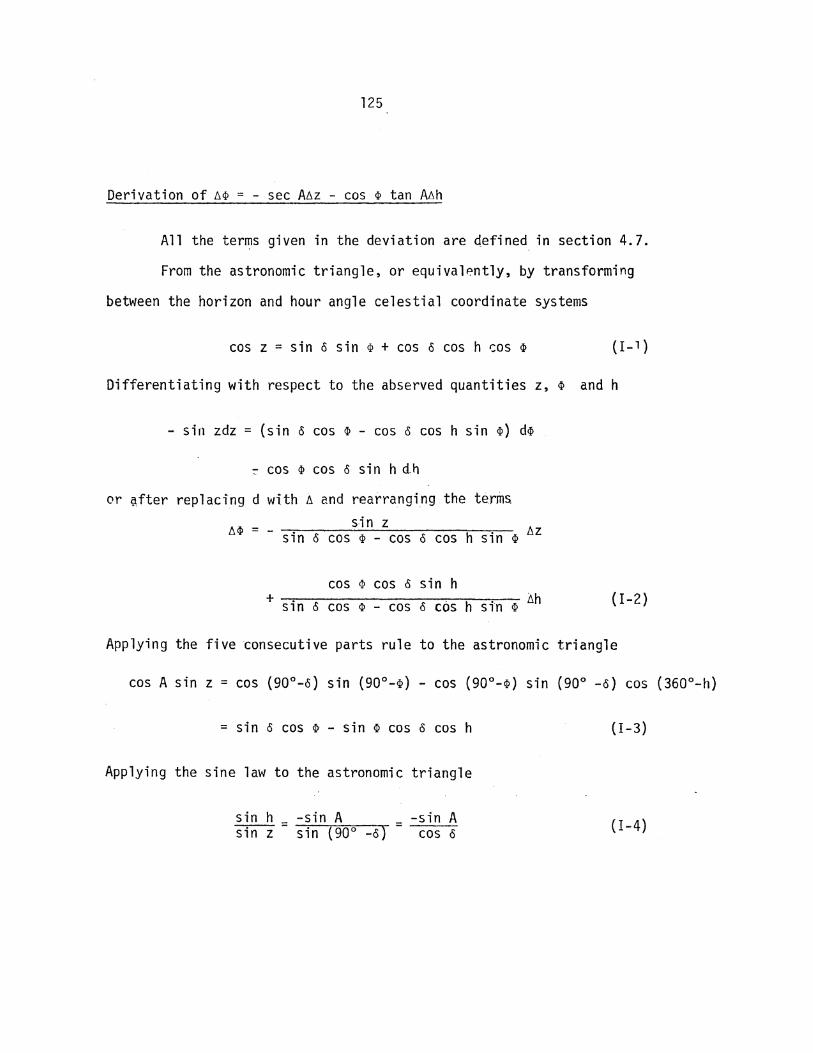
125
Derivation of ~~ = - sec A~z - cos ~ tan AAh
All the terms given in the deviation are ~efined_ in section 4.7.
From the astronomic triangle, or equival~ntly, by transforming
between the horizon and hour angle celestial coordinate systems
cos z = sin o sin ~ + cos o cos h cos ~ (I-1)
Differentiating with respect to the abserved quantities z, ~ and h
- sin zdz = (sin o cos ~ - cos o cos h sin ~) d~
7 cos ~ cos o sin h dh
or ~fter replacing d with fl and rearranging the terms. s-in z
fl~ = - sin o cos ~ - cos o cos h sin ~ flz
cos ~ cos o sin h + sin o cos ~ - cos o c6s h sin ~ Ah (I-2)
Applying the five consecutive parts rule to the astronomic triangle
= sin o cos ~ sin ~ cos o cos h (I-3)
Applying the sine law to the astronomic triangle
sin h _ -sin A = -sin A sin z - sin ( 90° -ol cos o {I-4)

126
Substituting cos A sin z for (sin o cos ~ - sin ~ cos o cos h) from
(I-3) and- sin A sin z for sin h from (I-4) into (I-2), and cos 0
simplifying yields
~~ = - sec A ~z - cos ~ tan A ~h (I-5)
Derivation of ~A = - sec ~ cot A ~~ - sec ~ cosec A ~z + ~T
All the terms given in the derivation are defined in Section
4.7.
From the astronomic triangle, or equivalently, by transforming
between the horizon and hour angle coordinate systems
A =a.+h-T (I-6)
Differentiating with respect to the observed quantities ~. h and T
di\ = dh - dT (I-7)
Replacing d with i1 and substituting (M· + 6T} for h from (I-7) it.to
'(·1-:-5}. and si.mplifying yields
~A = -.sec ~ cot A~~ - sec ~cosec A ~z + ~T (I-8)

127
HP-29C Program for ~A
The appropriate formula, in whch all terms are defined in
section 4.7, is
where
and
~A = - sec ~ cot A ~~ - sec ~ esc A ~z
A= cos-1 (sin o - cos z sin ~ ) sin z cos ~
z + z z = 1 2 2 + refraction correction
~ (0 I II)' o( 0 • 11 ), ~~( 11 ) and the refraction correction
(II) are stored as shown in the program listing.
The step by step program listing follows.
+~nter z( 11 ), z1( 0 I 11), z2(o I II)
[1] LBLl [21] RCL4 (o) [41] RCL6 [2] -+H [22] sin [42] X [3] ST05·; [23] + [43] CHS [4] R+ [24] RCLO [44] RCL7 (M) [5] -+H [25] ·cos [45] RCL8 [6] RCL5:; [26] RCL5 [46] tan [7] + [27] sin [47] 1/x [8] 2. [28] X [48] X [9] ..:. [29] . [49] RCLO -[10] RCL9_ (refr. carr.) [30] cos-1 [50] cos [11 J + [31] CHS / [51] 1/x [12] STC5 [32] 360 ( for WPVC only [52] X [13] R+ [33] + ~ [53] CHS [14] ST06·· · [34] s"ro8 [54] + [15] RCLO (~) [35] sin [55] RTN + displays ~A [16] sin [36] 1/x [17] RCL5 [37] RCLO [18] cos [38] cos [19] }( [39] 1/x [20] CHS [40] X