Geodesic shape regression in the

framework of currents

James Fishbaugh1, Marcel Prastawa1, Guido Gerig1, and Stanley Durrleman2

1 Scientific Computing and Imaging Institute, University of Utah2 INRIA/ICM, Pitie Salpetriere Hospital, Paris, France

Abstract. Shape regression is emerging as an important tool for thestatistical analysis of time dependent shapes. In this paper, we developa new generative model which describes shape change over time, by ex-tending simple linear regression to the space of shapes represented as cur-rents in the large deformation diffeomorphic metric mapping (LDDMM)framework. By analogy with linear regression, we estimate a baselineshape (intercept) and initial momenta (slope) which fully parameterizethe geodesic shape evolution. This is in contrast to previous shape re-gression methods which assume the baseline shape is fixed. We furtherleverage a control point formulation, which provides a discrete and low di-mensional parameterization of large diffeomorphic transformations. Thisflexible system decouples the parameterization of deformations from thespecific shape representation, allowing the user to define the dimension-ality of the deformation parameters. We present an optimization schemethat estimates the baseline shape, location of the control points, andinitial momenta simultaneously via a single gradient descent algorithm.Finally, we demonstrate our proposed method on synthetic data as wellas real anatomical shape complexes.

1 Introduction

Shape regression is of crucial importance for statistical shape analysis. It isuseful to find correlations between shape configuration and a continuous scalarparameter such as age, disease progression, drug delivery, or cognitive scores.When only few follow-up observations are available, regression is also a necessarytool to interpolate between data points and provide a scenario of continuousshape evolution over the parameter range [5,13]. Longitudinal studies also requireto compare such regressions across different subjects [5,8,10,11].

Extending traditional scalar regression for shape is not straightforward asshape intrinsically live on a Riemannian manifold. Therefore, methods differaccording to the choice of metric on the shape space and the corresponding re-gression function. In [5], a piecewise geodesic method has been proposed, whichextends piecewise linear regression for shape time-series. In [7,16] second-ordermodels have been proposed which are controlled by the acceleration of shapechanges or the deviation from geodesic paths. Non-parametric regression hasbeen proposed in [3], extending kernel regression to Riemannian manifolds. In [9]

geodesic regression is proposed as a straightforward extension of linear regres-sion on Riemannian manifolds. Geodesic regression is fully characterized by thebaseline shape (the intercept) and the tangent vector defining the geodesic at thebaseline shape (the slope). Therefore, it seems well adapted for longitudinal stud-ies, since different regressions could be compared by transporting baseline andtangent vectors from subject to subject, using parallel transport for instance [12].

Methods in [5,7,14] are based on the large deformation diffeomorphic metricmapping (LDDMM) paradigm, which is well suited for regression purposes sinceit is built on a continuous flow of diffeomorphisms that model continuous shapechanges over a time period. In [14], geodesic regression is proposed in the LD-DMM framework for image data. Extending it for geometric data such as curvesand surfaces is challenging for at least two reasons.

First, images seen as measures on R3 inherit from a linear structure which

eases the estimation of the baseline image (images could be averaged by aver-aging grey levels for instance). Curves or surfaces could be also embedded intoa vector space if we assume point correspondences between shapes [2]. Alterna-tively, we can avoid explicit correspondence by embedding shapes into the spaceof currents, which defines a generic metric which can handle both surfaces andcurves or any mix of them. However, the average of surfaces in the space of cur-rents is usually not a surface anymore [5]. To overcome this limitation, we willuse here the new formulation initiated in [6], which allows to optimize a giventemplate in the space of currents, while preserving its topology.

Second, the parameterization of the deformations in the LDDMM settingis given by a scalar momenta map (which plays the role of the tangent vectordefining the geodesic path), which has the same dimension as the images. Forpoint data, the parameterization is given by one momentum vector at everypoint of the baseline shape. The dimension of this parameterization explodeswhen shape complexes are analyzed. To overcome this limitation, we will usethe control point formulation in the LDDMM setting that has been introducedin [4]. Consequently, our geodesic model characterizes complex evolution witha small number of parameters (defined by the user), compared to [5,7] whichrequire vectors at every shape point and every time point in the discretization.

2 Methods

2.1 Shape regression

In shape regression, the goal is to estimate a continuous shape evolution from adiscrete set of observed shapes Oti at time ti within the time interval [t0, T ].Here we consider shape to be generic geometric objects that can be representedas curves, landmark points, or surfaces in 2D or 3D. Shape evolution is modeledas the geodesic flow of diffeomorphisms acting on a baseline shape X0, definedas X(t) = φt(X0) with t varying continuously within the time interval deter-mined by the observed data. The baseline shape X0 is continuously deformedover time to match the observation data (X(ti) ∼ Oti) with the rigidity of the

evolution controlled by a regularity term. This setting is naturally expressed asa variational problem, described by the regression criterion

E(X0, φt)) =

Nobs∑

i=1

||(φti(X0)−Oti)||2W∗ +Reg(φt)

=

Nobs∑

i=1

D(X(ti),Oti) + L(φt) (1)

where D represents the squared distance on currents (||·||2W∗) and L is a measureof the regularity of the time-varying deformation φt.

2.2 Control point parameterization of deformations

We adopt a discrete parameterization of deformations, where dense diffeomor-phisms of the underlying space are built by interpolating momenta located atcontrol points [4]. Let c0 = {c1, ..., cNc

} be a finite set of control points whichcarry initial momenta vectors α0 = {α1, ...αNc

}, together referred to as theinitial state of the system S0 = {c0,α0}.

The set of control point positions c0 and initial momenta α0 serve as initialconditions for the geodesic equations, which define the time evolution of thesystem of control points and momenta, given by

ci(t) =

Nc∑

p=1

K(ci(t), cp(t))αp(t)

αi(t) = −

Nc∑

p=1

αi(t)tαp(t)∇1K(ci(t), cp(t))

(2)

where K is the interpolating kernel assumed (without loss of generality) to beGaussian: K(x, y) = exp(−|x− y|2)/σ2). These equations describe the evolutionof the state of the system S(t) = {ci(t), αi(t)} and can be written in short asS(t) = FS(t)

Thanks to the geodesic equations, the trajectories of control points ci(t) andαi(t) now parameterize the time-varying velocity field v(x, t) defined at any pointin space x and time t as

x(t) = v(x, t) =

Nc∑

p=1

K(x, cp(t))αp(t). (3)

which can be written in short as x(t) = G(x(t),S(t)).The time-varying velocity field v(x, t) can then be used to build the flow

of deformations φt(x) in the spirit of the LDDMM framework by integratingthe ODE: φt(x) = v(φt(x), t). Using the coordinates of the baseline shape X0

as initial conditions, integrating this ODE computes the deformation of thebaseline shape from time t0 to T . Therefore the flow of diffeomorphisms is fullydetermined by the initial state of the system S0: the set of initial control pointsc0 and initial momenta vectors α0.

2.3 Minimization of regression criterion

Fig. 1. Overview ofgeodesic regressionwith estimated pa-rameters in red.

The geodesic flow of diffeomorphisms φt in the criterion (1)is parameterized by Nc control points and momenta vectorsS0 = {c0,α0}, which act as initial conditions for the flowequations (2). The baseline shape X0 can then be deformedaccording to this flow by applying equation (3). Thereforewe seek to estimate the position of the control points, initialmomenta, and position of the points on the baseline shapesuch that the resulting geodesic flow of the baseline shapebest matches the observed data. An overview of our controlpoint formulation of geodesic shape regression is shown inFig. 1. With all elements of our framework defined, geodesicshape regression can now be described by the specific regres-sion criterion

E(X0,S0) =

Nobs∑

i=1

1

2λ2D(X(ti),Oti) + L(S0) (4)

subject to{

S(t) = F (S(t)) with S(0) = {c0,α0}

X(t) = G(X(t),S(t)) with X(0) = X0(5)

where λ2 is used to balance the importance of the data term and regularity,L(S0) =

∑

p,q αt0,pK(c0,p, c0,q)α0,q is the regularity term defined by the kinetic

energy of the control points. The first part of (5) describes the trajectory of thecontrol points and momenta as in (2). The second equation of (5) representsflowing the baseline shape along the deformation defined by S(t) as in (3).

As shown in the appendix, the gradients of the criterion (4) are

∇S0E = ξ(0) +∇S0

L ∇X0E = θ(0) (6)

where the auxiliary variables θ(t) and ξ(t) = {ξc, ξα} satisfy the ODEs:

θ(t) = −∂1G(t)tθ(t) +

NObs∑

i=1

∇X(ti)D(ti)δ(t− ti) θ(T ) = 0

ξ(t) = −(∂2G(t)tθ(t) + dS(t)F (t)tξ(t)) ξ(T ) = 0

(7)

The gradient is computed by first integrating equations (2) forward in timeto construct the flow of diffeomorphisms. The deformations are then applied tothe baseline shape by integrating forward in time equation (3). With the fulltrajectory of the deformed baseline shape, one can compute the gradient of thedata term ∇X(ti)D(ti), corresponding to each observation. The ODEs (7) arethen integrated backwards in time, with the gradients of the data term actingas jump conditions at observation time points, which pull the geodesic towardstarget data. The final values of the auxiliary variables θ(0) and ξ(0) are thenused to update the location of the control points, the initial momenta, and thelocation of the points on the baseline shape.

The method, summarized in Algorithm 1, is implemented via a gradient de-scent scheme. The parameters of the algorithm are the tradeoff between datamatching and regularity λ, the standard deviation of the deformation kernel σV ,and the standard deviation of the metric on currents σW . The value of σV con-trols the scale at which points in space move in a correlated manner, while thevalue of σW controls the scale at which shape differences are considered noise.The algorithm also requires an initial baseline shape. For surfaces, initializationconsists of an ellipsoid for each connected component of the shapes, which de-fines the number of shape points as well as the connectivity, which is preservedduring optimization.

Algorithm 1: Geodesic shape regression

Input: X0 (initial baseline shape), Oti (observed shapes), t0 (start time), T(end time), σ (tradeoff), σV (std. dev. of deformation kernel), σW (std.dev. of currents metric)

Output: X0, c0,α0

1 α0 ← 02 Initialize control points c0 on regular grid with spacing σV

3 repeat4 {Compute path of control points and momentum (forward integration)}

5 ci(t) = ci(0) +∫ T

t0

∑Nc

p=1 K(ci(s), cp(s))αp(s)ds

6 αi(t) = αi(0)−∫ T

t0

∑Nc

p=1 αi(s)tαp(s)∇1K(ci(s), cp(s))ds

7 {Compute trajectory of deformed baseline shape (forward integration)}

8 xk(t) = xk(0) +∫ T

t0

∑Nc

p=1 K(xk(s), cj(s))αj(s)ds

9 {Compute the gradient of the data term for each observation}10 ∇X(ti)D(ti)11 {Compute auxiliary variable θ(t) (backward integration)}

12 θk(t) = θk(T ) +∫ t

T

∑Nc

p=1 αp(s)tθk(s)∇1K(xk(s), cp(s)) −

13

∑Nobs

i=1 ∇xk(ti)Dδ(s− ti)ds14 {Compute auxiliary variable ξc(t) (backward integration)}

15 ξck(t) = ξck(T )−∫ t

T

∑Nx

p=1 αk(s)tθp(s)∇1K(ck(s), xp(s)) +

16 (∂cFc)ξck(s) + (∂cF

α)ξαk (s)ds17 {Compute auxiliary variable ξα(t) (backward integration)}

18 ξαk (t) = ξαk (T )−∫ t

T

∑Nx

p=1 K(ck(s), xp(s))θp(s) +

19 (∂αFc)ξck(s) + (∂αF

α)ξck(s)ds20 {Compute gradients}21 ∇c0

E = ξc(0) +∇c0L

22 ∇α0E = ξα(0) +∇α0

L

23 ∇X0E = θ(0)

24 {Update control points, momenta, and baseline shape}25 ci(0)← ci(0)− ε∇ciE αi(0)← αi(0)− ε∇αi

E xi(0)← xi(0)− ε∇xiE

26 until Convergence27 return X0, c0,α0

3 Results

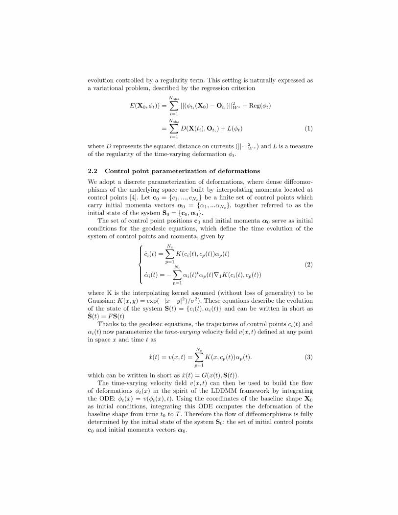
Fig. 2. Initial baseline shapeand observed amygdala.

Synthetic Transformations We explore the abil-ity of the geodesic regression model to capturesimple synthetic transformations applied to a realanatomical surface. We consider the amygdala sur-face extracted from a 4 year old child and investi-gate translation and scaling. For both experiments,we initialize the baseline shape to be an ellipse, asshown in Fig. 2, which defines the topology of thebaseline shape, which will remain unchanged dur-ing optimization. We define 12 control points on aregular grid and parameters σV = 12 mm, σW = 5 mm, and λ = 0.1. Bothexperiments contain three shape observations spaced one time unit apart.

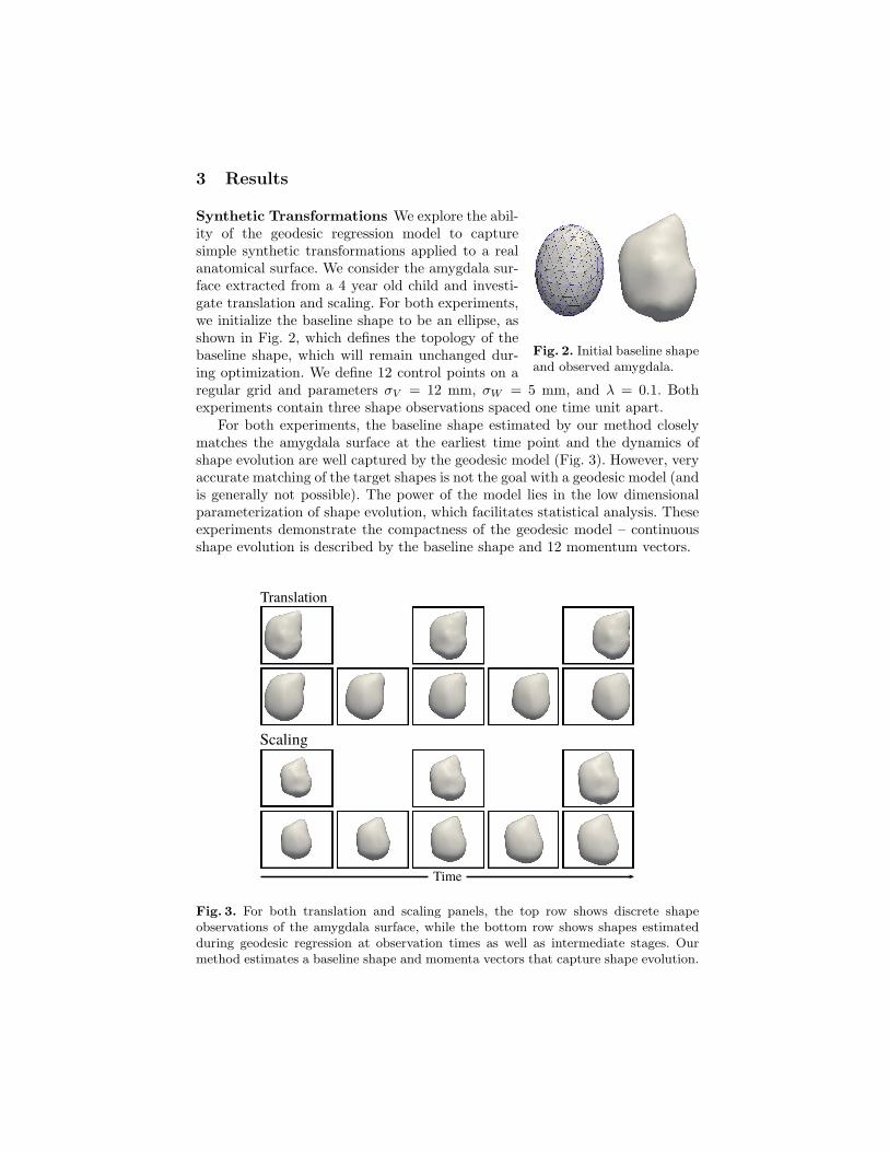
For both experiments, the baseline shape estimated by our method closelymatches the amygdala surface at the earliest time point and the dynamics ofshape evolution are well captured by the geodesic model (Fig. 3). However, veryaccurate matching of the target shapes is not the goal with a geodesic model (andis generally not possible). The power of the model lies in the low dimensionalparameterization of shape evolution, which facilitates statistical analysis. Theseexperiments demonstrate the compactness of the geodesic model – continuousshape evolution is described by the baseline shape and 12 momentum vectors.

Fig. 3. For both translation and scaling panels, the top row shows discrete shapeobservations of the amygdala surface, while the bottom row shows shapes estimatedduring geodesic regression at observation times as well as intermediate stages. Ourmethod estimates a baseline shape and momenta vectors that capture shape evolution.

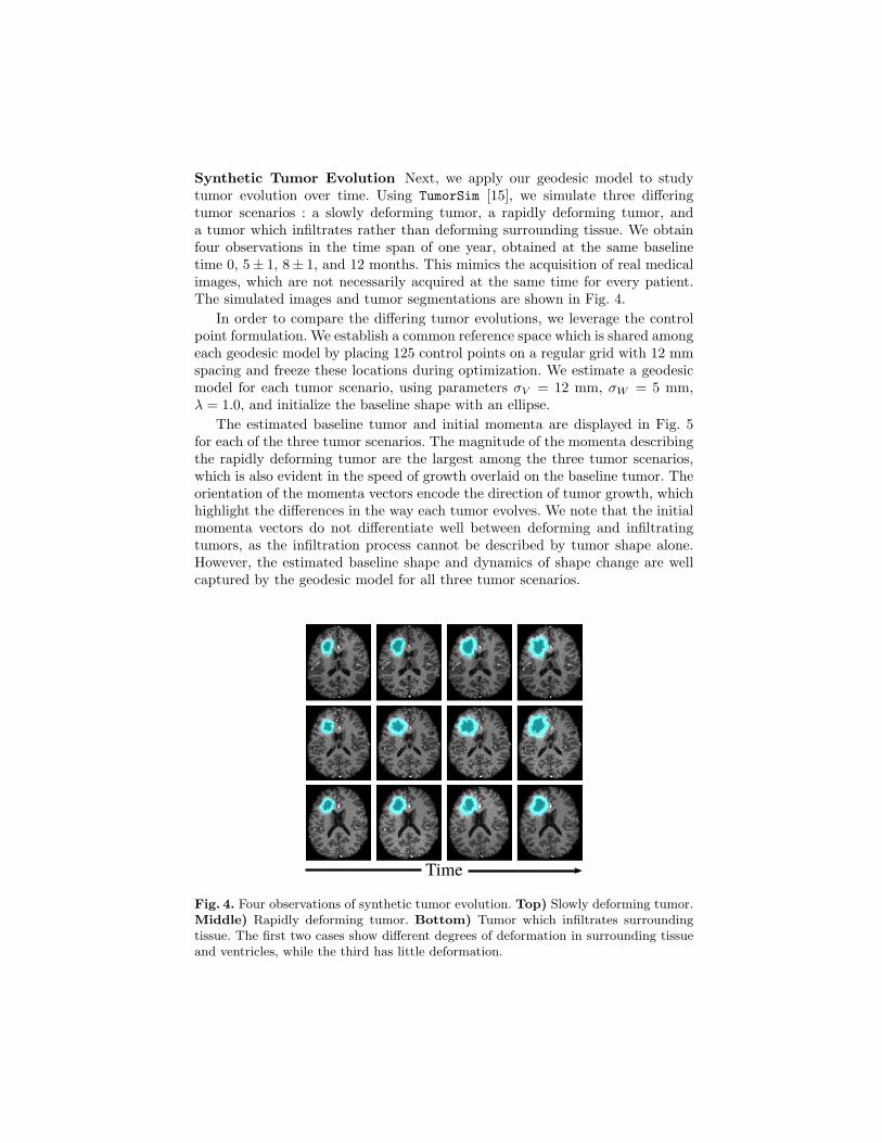
Synthetic Tumor Evolution Next, we apply our geodesic model to studytumor evolution over time. Using TumorSim [15], we simulate three differingtumor scenarios : a slowly deforming tumor, a rapidly deforming tumor, anda tumor which infiltrates rather than deforming surrounding tissue. We obtainfour observations in the time span of one year, obtained at the same baselinetime 0, 5± 1, 8± 1, and 12 months. This mimics the acquisition of real medicalimages, which are not necessarily acquired at the same time for every patient.The simulated images and tumor segmentations are shown in Fig. 4.

In order to compare the differing tumor evolutions, we leverage the controlpoint formulation. We establish a common reference space which is shared amongeach geodesic model by placing 125 control points on a regular grid with 12 mmspacing and freeze these locations during optimization. We estimate a geodesicmodel for each tumor scenario, using parameters σV = 12 mm, σW = 5 mm,λ = 1.0, and initialize the baseline shape with an ellipse.

The estimated baseline tumor and initial momenta are displayed in Fig. 5for each of the three tumor scenarios. The magnitude of the momenta describingthe rapidly deforming tumor are the largest among the three tumor scenarios,which is also evident in the speed of growth overlaid on the baseline tumor. Theorientation of the momenta vectors encode the direction of tumor growth, whichhighlight the differences in the way each tumor evolves. We note that the initialmomenta vectors do not differentiate well between deforming and infiltratingtumors, as the infiltration process cannot be described by tumor shape alone.However, the estimated baseline shape and dynamics of shape change are wellcaptured by the geodesic model for all three tumor scenarios.

Fig. 4. Four observations of synthetic tumor evolution. Top) Slowly deforming tumor.Middle) Rapidly deforming tumor. Bottom) Tumor which infiltrates surroundingtissue. The first two cases show different degrees of deformation in surrounding tissueand ventricles, while the third has little deformation.

Fig. 5. Baseline shape and initial momenta for geodesic models of tumor evolution.Our regression framework captures the different tumor growth characteristics, withmomenta vectors constrained to be in the same coordinates for comparison purposes.

Pediatric Subcortical Development We next investigate the application ofgeodesic shape regression to model pediatric subcortical development. Three sub-cortical shapes are considered as a multi-object shape complex: putamen, amyg-dala, and hippocampus. The structures were obtained from MRI of a healthychild scanned at approximately 9, 13, and 24 months of age. Geodesic regressionwas conducted using 126 control points and parameters σV = 8 mm, σW = 6mm, and λ = 1.0. To improve speed of convergence, we initialize the baselineshapes for each subcortical structure with an ellipse that has been coarsely reg-istered to its corresponding subcortical shape. Regression was conducted on allshapes simultaneously, resulting in one deformation of the ambient space.

Several snapshots of the evolution of subcortical structures is shown in Fig.6, with estimated baseline shape shown at 6 months. From 6 to 26 months,all subcortical structures increase in size, with the putamen demonstrating themost dramatic growth. The evolution of the putamen is characterized by ac-celerated growth at the superior anterior and inferior posterior regions, whilethe hippocampus grows mostly at the extreme posterior region, expanding andbending at the tip. The geodesic model is able to capture interesting non-lineargrowth patterns with few parameters; the full time evolution is modeled by threebaseline shapes and 126 momenta vectors.

This experiment demonstrates the applicability of the geodesic model in char-acterizing pediatric subcortical development. Our regression framework simulta-neously handles multiple shapes, including those with complex geometry. Multi-object regression allows for a more complete analysis, compared to an indepen-dent treatment of each subcortical structure, which ignores potentially importantspatial relationships between structures. This single subject experiment can alsobe extended to a population analysis thanks to the control point formulation ofdeformations. As with the previous tumor experiment, one can fix the controlpoint locations for all subjects. The differences between and within populations

Fig. 6. Snapshots of subcortical shape evolution after geodesic regression on a multi-object complex: putamen, amygdala, and hippocampus.

can be quantified by exploring the variability between estimated baseline shapes,and between initial momenta at identical locations for all subjects.

White Matter Fibers in Early Brain Development Finally, we study earlybrain development by considering the evolution of white matter connections frombirth to 2 years of age. For this experiment, we have diffusion tensor imaging(DTI) data from 17 subjects with scans obtained at clustered time points of2± 2, 12± 2 months, and 24± 2 months. We extract the genu fiber tract fromeach DTI using the framework of [1]. In our experiment, we use 26 genu fibertracts which are represented as a collection of 3D curves. By considering fibergeometry obtained from multiple subjects, the estimated geodesic model canbe considered as the development of the genu tract for an average child. Weinitialize the baseline shape with the genu fiber bundle from the atlas space,define 75 control points on a regular grid, and set parameter values as σV = 5mm, σW = 8 mm, and λ = 0.1.

The average development of the genu tract estimated by our geodesic model issummarized in Fig. 7, which shows several snapshots on the genu fibers over time.The elongation of the fibers reflects the myelination process that occur duringearly development, where myelin sheaths grows to cover white matter regionsoutward to the cortex. Our geodesic regression framework handles the multiplefiber structure that form the genu fiber bundle, using the currents framework tomatch the curvilinear fiber structures.

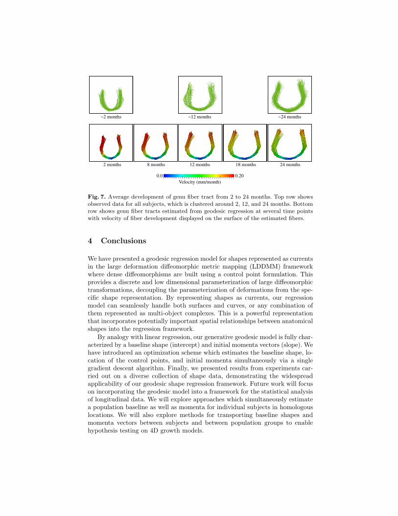
Fig. 7. Average development of genu fiber tract from 2 to 24 months. Top row showsobserved data for all subjects, which is clustered around 2, 12, and 24 months. Bottomrow shows genu fiber tracts estimated from geodesic regression at several time pointswith velocity of fiber development displayed on the surface of the estimated fibers.

4 Conclusions

We have presented a geodesic regression model for shapes represented as currentsin the large deformation diffeomorphic metric mapping (LDDMM) frameworkwhere dense diffeomorphisms are built using a control point formulation. Thisprovides a discrete and low dimensional parameterization of large diffeomorphictransformations, decoupling the parameterization of deformations from the spe-cific shape representation. By representing shapes as currents, our regressionmodel can seamlessly handle both surfaces and curves, or any combination ofthem represented as multi-object complexes. This is a powerful representationthat incorporates potentially important spatial relationships between anatomicalshapes into the regression framework.

By analogy with linear regression, our generative geodesic model is fully char-acterized by a baseline shape (intercept) and initial momenta vectors (slope). Wehave introduced an optimization scheme which estimates the baseline shape, lo-cation of the control points, and initial momenta simultaneously via a singlegradient descent algorithm. Finally, we presented results from experiments car-ried out on a diverse collection of shape data, demonstrating the widespreadapplicability of our geodesic shape regression framework. Future work will focuson incorporating the geodesic model into a framework for the statistical analysisof longitudinal data. We will explore approaches which simultaneously estimatea population baseline as well as momenta for individual subjects in homologouslocations. We will also explore methods for transporting baseline shapes andmomenta vectors between subjects and between population groups to enablehypothesis testing on 4D growth models.

Acknowledgments. This work was supported by NIH grant RO1 HD055741(ACE, project IBIS) and by NIH grant U54 EB005149 (NA-MIC).

References

1. Basser, P., Pajevic, S., Pierpaoli, C., Duda, J., Aldroubi, A.: In vivo fiber tractog-raphy using DT-MRI data. Magnetic resonance in medicine 44(4), 625–632 (2000)

2. Datar, M., Cates, J., Fletcher, P., Gouttard, S., Gerig, G., Whitaker, R.: Particlebased shape regression of open surfaces with applications to developmental neu-roimaging. In: Yang, G.Z., Hawkes, D.J., Rueckert, D., Noble, J.A., Taylor, C.J.(eds.) MICCAI 2009, Part II. LNCS, vol. 5762, pp. 167–174. Springer (2009)

3. Davis, B., Fletcher, P., Bullitt, E., Joshi, S.: Population shape regression fromrandom design data. In: ICCV. pp. 1–7. IEEE (2007)

4. Durrleman, S., Allassonniere, S., Joshi, S.: Sparse adaptive parameterization ofvariability in image ensembles. IJCV pp. 1–23 (2012)

5. Durrleman, S., Pennec, X., Trouve, A., Braga, J., Gerig, G., Ayache, N.: Toward acomprehensive framework for the spatiotemporal statistical analysis of longitudinalshape data. IJCV pp. 1–38 (2012)

6. Durrleman, S., Prastawa, M., Korenberg, J.R., Joshi, S.C., Trouve, A., Gerig, G.:Topology preserving atlas construction from shape data without correspondenceusing sparse parameters. In: Ayache, N., Delingette, H., Golland, P., Mori, K. (eds.)MICCAI. LNCS, vol. 7512, pp. 223–230. Springer (2012)

7. Fishbaugh, J., Durrleman, S., Gerig, G.: Estimation of smooth growth trajectorieswith controlled acceleration from time series shape data. In: Fichtinger, G., Peters,T. (eds.) MICCAI. LNCS, vol. 6892, pp. 401–408. Springer (2011)

8. Fishbaugh, J., Prastawa, M., Durrleman, S., Piven, J., Gerig, G.: Analysis of lon-gitudinal shape variability via subject specific growth modeling. In: Ayache, N.,Delingette, H., Golland, P., Mori, K. (eds.) MICCAI. LNCS, vol. 7510, pp. 731–738.Springer (2012)

9. Fletcher, P.: Geodesic Regression on Riemannian Manifolds. In: Pennec, X., Joshi,S., Nielsen, M. (eds.) MICCAI MFCA. pp. 75–86 (2011)

10. Hart, G., Shi, Y., Zhu, H., Sanchez, M., Styner, M., Niethammer, M.: DTI longi-tudinal atlas construction as an average of growth models. In: Gerig, G., Fletcher,P., Pennec, X. (eds.) MICCAI STIA (2010)

11. Liao, S., Jia, H., Wu, G., Shen, D.: A novel longitudinal atlas construction frame-work by groupwise registration of subject image sequences. NeuroImage 59(2),1275–1289 (2012)

12. Lorenzi, M., Ayache, N., Pennec, X.: Schilds ladder for the parallel transport ofdeformations in time series of images. In: Szekely, G., Hahn, H. (eds.) IPMI. LNCS,vol. 6801, pp. 463–474 (2011)

13. Mansi, T., Voigt, I., Leonardi, B., Pennec, X., Durrleman, S., Sermesant, M.,Delingette, H., Taylor, A.M., Boudjemline, Y., Pongiglione, G., Ayache, N.: Astatistical model for quantification and prediction of cardiac remodelling: Appli-cation to tetralogy of fallot. IEEE Trans. on Medical Imaging 9(30), 1605–1616(2011)

14. Niethammer, M., Huang, Y., Vialard, F.X.: Geodesic regression for image time-series. In: Fichtinger, G., Peters, T. (eds.) MICCAI. LNCS, vol. 6982, pp. 655–662.Springer (2011)

15. Prastawa, M., Bullitt, E., Gerig, G.: Simulation of brain tumors in mr images forevaluation of segmentation efficacy. Medical Image Analysis 13(2), 297–311 (2009)

16. Vialard, F., Trouve, A.: Shape splines and stochastic shape evolutions: A second-order point of view. Quarterly of Applied Mathematics 70, 219–251 (2012)

A Differentiation of the Regression Criterion

Consider a perturbation δS0 to the initial state of the system (c0, α0), whichleads to a perturbation of the motion of the control points δS(t), a perturbationof the template shape trajectory δX(t), and a perturbation of the criterion δE

δE =

Nobs∑

i=1

(

(∇X(ti)D(ti))tδX(ti)

)

+ (∇S0L)tδS0. (8)

The perturbations δS(t) and δX(t) satisfy the ODEs:

δS(t) = dS(t)F (t)δS(t) δS(0) = δS0

δX(t) = ∂1G(t)δX(t) + ∂2G(t)δS(t) δX(0) = δX0(9)

Let Rst = exp(

∫ t

sdS(u)F (u)du

)

and Vst = exp(

∫ t

s∂1G(u)du

)

. The first ODE

is a linear homogeneous ODE with well known solution

δS(t) = R0tδS0 (10)

The second ODE is a linear inhomogeneous ODE with solution

δX(ti) =

(∫ ti

0

Vuti∂2G(u)R0udu

)

δS0 + V0tiδX0 (11)

which can now be plugged into (8). After arranging terms we have

δE =

Nobs∑

i=1

[∫ ti

0

R0ut∂2G(u)tVuti

t∇X(ti)D(ti)du

]t

δS0 + [∇S0L]

tδS0

+

Nobs∑

i=1

[

V0tit∇X(ti)D(ti)

]tδX0

(12)

Letting θ(t) =∑Nobs

i=1 Vttit∇X(ti)D(ti)1{t≤ti}, g(t) = ∂2G(t)θ(t), and ξ(t) =

∫ ti

tRtu

tg(u)du leads to the gradient of the criterion written as

∇S0E =

∫ ti

0

R0utg(u)du+∇S0

L = ξ(0) +∇S0L

∇X0E = θ(0)

(13)

where auxiliary variables θ(t) and ξ(t) satisfy the ODEs

θ(t) = −∂1G(t)tθ(t) +

NObs∑

i=1

∇X(ti)D(ti)δ(t− ti) θ(T ) = 0

ξ(t) = −(∂2G(t)tθ(t) + dS(t)F (t)tξ(t)) ξ(T ) = 0.

(14)