gennaro d’angelo and matthew r. bate - arxiv · gennaro d’angelo and matthew r. bate ... in the...

arX

iv:a

stro

-ph/

0411

705v

1 2

5 N

ov 2

004

November 2004

The dependence of protoplanet migration rates on coorbital torques1

Gennaro D’Angelo and Matthew R. BateSchool of Physics, University of Exeter, Stocker Road, Exeter EX4 4QL, United Kingdom

[email protected], [email protected]

and

Steve H. LubowSpace Telescope Science Institute, 3700 San Martin Drive, Baltimore, MD 21218, USA

[email protected]

ABSTRACT

We investigate the migration rates of high-mass protoplanets embedded in accretion discs via two andthree-dimensional hydrodynamical simulations. The simulations follow the planet’s radial motion andemploy a nested-grid code that allows for high resolution close to the planet. We concentrate on thepossible role of the coorbital torques in affecting migration rates. We analyse two cases: (a) a Jupiter-massplanet in a low-mass disc and (b) a Saturn-mass planet in a high-mass disc. The gap in case (a) is muchcleaner than in case (b). Planet migration in case (b) is much more susceptible to coorbital torques than incase (a). We find that the coorbital torques in both cases do not depend sensitively on whether the planetis allowed to migrate through the disc or is held on a fixed orbit. We also examine the dependence of theplanet’s migration rate on the numerical resolution near the planet. For case (a), numerical convergenceis relatively easy to obtain, even when including torques arising from deep within the planet’s Hill sphere,since the gas mass contained within the Hill sphere is much less than the planet’s mass. The migration ratein this case is numerically on order of the Type II migration rate and much smaller than the Type I rate,if the disc has 0.01 solar-masses inside 26AU. Torques from within the Hill sphere provide a substantialopposing contribution to the migration rate. In case (b), the gas mass within the Hill sphere is largerthan the planet’s mass and convergence is more difficult to obtain. Torques arising from within the Hillsphere are strong, but nearly cancel. Any inaccuracies in the calculation of the torques introduced by griddiscretization can introduce spurious torques. If the torques within the Hill sphere are ignored, convergenceis more easily achieved but the migration rate is artificially large. At our highest resolution, the migrationrate for case (b) is much less than the Type I rate, but somewhat larger than the Type II rate.

Subject headings: accretion, accretion discs — hydrodynamics — planetary systems: formation, protoplanetarydiscs

1. Introduction

When the first planetary systems were discovered, migra-tion provided the natural explanation for the existence of theso-called “Hot Jupiters” (Lin, Bodenheimer & Richardson1996). For this explanation to hold, migration time-scalesshould be no longer than disc life-times of several millionyears (e.g., Haisch, Lada & Lada 2001). However, the migra-tion and planet formation processes are inter-related. Clearly,there would be complications and possibly difficulties in un-derstanding planet formation by a process whose time-scaleis long compared to the migration time-scale.

1To appear in the Monthly Notices of the Royal

Astronomical Society. A version with high resolutionfigures is available athttp://www.astro.ex.ac.uk/people/gennaro/publications/.

In the case of giant planet formation by the core accre-tion process (e.g., Bodenheimer & Pollack 1986; Wuchterl1991a), the formation time-scale of about 107 years (Pollacket al. 1996; Tajima & Nakagawa 1997) is rather long com-pared to migration time-scales of about 105 years (e.g., Lin &Papaloizou 1986; Ward 1997) for a Jupiter-mass planet andabout 106 years for an Earth-mass core (Tanaka, Takeuchi& Ward 2002; D’Angelo, Kley & Henning 2003; Bate et al.2003).

However, it has been found recently (Rice & Armitage2003; Alibert, Mordasini & Benz 2004) that the effects of ac-cretion and migration of a planetary core can significantlyreduce the time needed by the core to reach the mass neces-sary for the nucleated instability to occur (Wuchterl 1991b;Magni & Coradini 2004). Furthermore, several recent studieshave suggested that additional effects may be of importance

1

http://arxiv.org/abs/astro-ph/0411705v1

http://www.astro.ex.ac.uk/people/gennaro/publications/

2 Migration rates of protoplanets

to migration. These include thermal effects of the disc mate-rial near a planet (Morohoshi & Tanaka 2003; Jang-Condell& Sasselov 2004), effects of radial opacity jumps in the disc(Menou & Goodman 2004), effects of vortices induced by aplanet (Koller, Li & Lin 2003), effects of turbulent fluctu-ations (Nelson & Papaloizou 2004), and effects of coorbitalmaterial (Masset & Papaloizou 2003, hereafter MP03). Inthe current study, we consider effects of coorbital material,along the lines of MP03.

Corotation torques arise in the coorbital region. In theabsence of dissipation or other time-dependent effects, thecorotation torque is zero in a smooth disc. The reason is thatin a steady-state, fluid elements circulate in closed orbits.Over a libration time-scale, a fluid element will gain and losetorque, but the result is zero average torque. Formally, thecorotation region in linear theory gives rise to a torque thatdepends on the gradient of the disc vortensity (e.g., Goldreich& Tremaine 1979). This torque is properly interpreted asan “unsaturated” or maximal torque that arises over time-scales less than a libration time-scale or when the effects ofviscosity are sufficiently large in steady-state. A derivationthat includes nonlinear feedback shows that the steady-statecorotation torque is indeed zero for a fluid in a smooth invisciddisc (Balmforth & Korycansky 2001; Ogilvie & Lubow 2003,see also Masset 2001). But, even the unsaturated corotationtorque for typical planet-disc systems is somewhat smaller inmagnitude than the other (Lindblad) torques present (Tanakaet al. 2002). Furthermore, for typical disc parameters, thistorque is likely saturated (reduced to a smaller value), sincethe effects of turbulent viscosity are not sufficiently strong, atleast in an alpha model description.

The above-described analyses did not take into accountthe effects of the radial migration of the planet. This motionmay cause enough asymmetry in the corotational flow that anet torque occurs, which may lead to a “runaway” situation(MP03). That is, the migration of the planet might cause acorotational torque that enhances the migration rate, whichin turn further promotes asymmetry and leads to a strongertorque, etc. Examples of such a runaway phenomenon werereported in simulations by MP03. The most favourable cir-cumstances for such a process are expected when a planetinteracts with a massive disc in which there is not a cleangap.

In addition to the classical corotational torques that arisefrom nearly librating orbits, coorbital torques can also arisewithin the Hill sphere of the planet. Material flows intothis region and forms a circumplanetary disc with shocks(Lubow, Seibert & Artymowicz 1999; D’Angelo, Henning &Kley 2002).

Our previous studies did not allow the planet to migrateduring the course of the simulation and therefore could nothave found such a runaway migration. Numerical resolution isa key issue because densities near a planet are relatively highand fractionally small density errors there can give rise tolarge spurious torques. Bate et al. (2003) found that torquesnear the planet may contribute somewhat (∼ 20 per cent) tothe migration rate. However, that study lacked the resolutionto reliably determine such torques.

In this paper, we investigate if the torques exerted on a

high-mass planet by a disc depend significantly on whetherthe planet is kept on a fixed orbit or allowed to migrate.We also investigate the possible role of torques due to ma-terial within the Hill sphere. We do this by means of two-dimensional (2D) and three-dimensional (3D) high resolutionhydrodynamical simulations. A key feature of the code isthat it allows high resolution to be achieved by means ofnested grids that encompass a region around the planet asit migrates. With this code, we are able to examine the con-tribution of the material inside the planet’s Hill sphere to thetotal torque on the planet.

The outline of the paper is as follows. In Section 2 thephysical model is described. In Section 3 we present anoverview of the numerical procedures employed in these com-putations. The results of the calculations are provided inSections 4 and 5. In Section 6 we present a discussion ofthese results and our conclusions.

2. Description of the physical model

It is generally believed that the interaction between a cir-cumstellar disc and a Jupiter-sized object can be studied bymeans of a two-dimensional approximation (Kley, D’Angelo& Henning 2001; D’Angelo et al. 2003). However, while this ispossibly true when considering interactions occurring at Lind-blad resonance locations (i.e., at distances from the planetlarger than a disc scale-height, H), it is not yet clear whetheror to what extent this remains a valid assumption when deal-ing with other interactions occurring at coorbital locations(Masset 2002). Therefore, in this investigation we consideredboth 2D and 3D disc models.

In the 2D geometry we employed a cylindrical coordinateframe O; r, φ, z, with the disc confined in the plane z = 0,whereas in the 3D geometry we used a spherical polar coor-dinate frame O;R, θ, φ. The rotational axis of the disc iseither parallel to the z-axis or to the polar direction, θ = 0.Both reference frames have their origin, O, on the star androtate about the disc axis with an angular velocity Ω andan angular acceleration Ω, being this last vector also parallelto the disc axis. The magnitudes of Ω and Ω are specifiedlater in this section. For the sake of clarity we point out that,whenever the variable r is used in the context of spherical po-lar coordinates, it indicates the distance from the rotationalaxis r = R sin θ.

2.1. Equations of motion for the disc

The hydrodynamical equations describing the disc evolu-tion are usually written in the conservative form for the radialand angular momenta. This can be derived from the Navier-Stokes equations for the velocities (see, e.g., Mihalas &WeibelMihalas 1999, Chapter 3) and the continuity equation. Sincethe 2D equations in cylindrical coordinates can be formallyderived from the 3D equations in spherical polar coordinates,we explicitly write them only for the latter reference frame.Indicating with ρ the mass density, with u ≡ (uR, uθ, uφ)the fluid velocity, and with ωA = ω + Ω the absolute angu-lar velocity of the fluid around the disc axis (ω r = uφ), theequations of motion for the disc in conservative form can be

G. D’Angelo, M. Bate, & S. Lubow 3

written as∂ρ

∂t+∇ · (ρu) = 0, (1)

∂ξR∂t

+∇·(ξR u) = ρ (u2θ

R+ω2

A R sin2 θ)−∂p

∂R−ρ

∂Φ

∂R+fR, (2)

∂ξθ∂t

+∇ · (ξθ u) = ρ ω2A R2 sin 2 θ

2−

∂p

∂θ− ρ

∂Φ

∂θ+Rfθ , (3)

∂ξφ∂t

+∇ · (ξφ u) = −∂p

∂φ− ρ

∂Φ

∂φ+R sin θ fφ, (4)

where(ξR, ξθ, ξφ) = ρ (uR, uθ R,ωA R2 sin2 θ) (5)

are the radial and angular momentum densities. Equationsin 2D cylindrical coordinates can be obtained from equa-tions (1), (2), (4), and (5) by replacing ρ with the surfacedensity Σ, using the appropriate expression for the divergenceoperator, dropping all terms that contain the velocity uθ, andsetting θ = π/2.

Note that ξφ is the absolute azimuthal angular momentum(density) of the fluid rather than that relative to the rotatingreference frame. This basically means that the non-inertialterms arising from the rotation of the reference frame (i.e.,Coriolis and angular velocity accelerations) are incorporatedin the left-hand side of equation (4). This choice assures abetter numerical treatment of the associated conservation law(Kley 1998).

We adopted a locally isothermal equation of state by set-ting p = c2s ρ (or p = c2s Σ in 2D) . The sound speed, cs, isequal to the disc aspect ratio, H/r, times the Keplerian ve-locity, vK. We used a constant disc aspect ratio throughoutthe disc, implying that the temperature distribution scales asthe inverse of the distance from the disc axis.

Since self-gravity is ignored, the gravitational potential,Φ,only includes contributions from the star, the planet, and thenon-inertial forces arising from the motion of the frame origin,O. Indicating the position vector of a fluid element as x andthat of the planet as xp, the disc gravitational potential reads

Φ = −GM∗

|x|−

GMp√

|x − xp|2 + ε2+

GMp

|xp|3x · xp, (6)

where M∗ is the stellar mass, Mp is the planet mass, andε is a smoothing length (see the discussion in section 2.4).The third term on the right-hand side of equation (6) origi-nates from the fact that the origin of the coordinate frame isaccelerated by the planet2.

The viscosity force density, f ≡ (fR, fθ , fφ) (or f ≡(fr, fφ) in 2D), is written as f = ∇ · S. It assumes a stan-dard viscous stress tensor, S, for a Newtonian fluid with aconstant kinematic viscosity, ν, and a zero bulk viscosity. Ex-plicit forms for the components of f can be found in Mihalas& Weibel Mihalas (1999, Chapter 3), for the 3D sphericalpolar coordinates case and in D’Angelo et al. (2002), for the2D cylindrical coordinates case.

2To be strict, an additional term should appear in equation (6)due to the force exerted by the disc material on to the star, asmeasured from the centre-of-mass reference frame. We neglectedthis contribution, as is done when assuming that the centre-of-massof the whole system coincides with that of the star–planet system.

2.2. Equation of motion for the planet

In the present study the planet’s orbit evolves under thegravitational action of the central star and of the disc mate-rial. Moreover, since the orbit is described with respect toa varying rotating reference frame, all non-inertial terms in-volving the angular velocity, Ω, and the angular acceleration,Ω, of the coordinate system have to be taken into account.Restricting to those orbits coplanar with the disc midplane

(θ = π/2 or z = 0), the equation of motion of the planet is

xp = −G(M∗ +Mp)

|xp|3xp +Ap −A∗ (7)

−Ω× (Ω× xp)− 2Ω× xp − Ω× xp.

We recall that, by working hypothesis, Ω as well as Ω areperpendicular to the disc midplane and produce a counter-clockwise rotation. The acceleration applied by the disc mat-ter to the planet is given by

Ap = G

∫

MD

(x − xp) dMD(x)

(|x − xp|2 + ε2)3/2, (8)

while the acceleration applied to the star is

A∗ = G

∫

MD

x dMD(x)

|x|3. (9)

In both cases the integration is carried out over the simulateddisc mass, MD (see section 2.4).

Equation (8) contains the smoothing length in its denomi-nator. This expression for acceleration appears in the secondterm of equation (6). An acceleration with smoothing is ap-plied to the planet’s motion in order to satisfy Newton’s thirdlaw.

2.3. Rotational elements of the reference frame

The main aim of this paper is to study the exchange ofangular momentum occurring between a migrating planet anddisc material moving on U-turns of horse-shoe orbits. In orderto accurately resolve the flow variables in this region by meansof a local grid-refinement technique, the planet needs to movethrough the grid as slowly as possible. To achieve this, weworked in reference frames that rotate about the disc axis ata variable rate, Ω = Ω(t). We then chose Ω and Ω so as tocompensate for the fastest component of the planet motion,i.e., the azimuthal one. This is accomplished by calculatingthe total orbital angular momentum of the planet per unitmass, HA, and then requiring that

HA = xp × (Ω× xp), (10)

HA = xp × (Ap −A∗). (11)

These equations are to be solved with the additional require-ments that both Ω and Ω must be perpendicular to the planeof the orbit and produce a positive (i.e., counter-clockwise)rotation. Equations 10 and 11 constrain the angular veloc-ity and acceleration of the rotating coordinate system so thatthe planet trajectory reduces to a purely radial motion. Inother terms, all of the planet’s orbital angular momentum isconveyed to the rotation of the non-inertial reference frame.


If the orbital eccentricity remains close to zero during thesystem evolution, as we found in our simulations, then theplanet’s radial motion is only due to the disc gravitationaltorques. We denote the planet’s semi-major axis as a = |xp|and the time-scale of this drifting motion as τM = a/|a|. Thequantity Nr ∆r (or NR ∆R) is the radial extent of the high-est refinement region and the time spent within this regionis Nr ∆r/|a| = Nr (∆r/a) τM, which is on the order of 0.1 τMfor the parameters used in the calculations. Numerical sim-ulations (e.g., Lubow et al. 1999; Nelson et al. 2000; Kleyet al. 2001; D’Angelo et al. 2002) as well as analytical the-ories (Goldreich & Tremaine 1980; Lin & Papaloizou 1986;Ward 1997) on disc torques suggest time-scales, τM, on theorder of 104 periods. Therefore, with this method one canexpect to track the planet and the coorbital regions, with thenecessary numerical resolution, for hundreds of orbits.

2.4. Physical parameters

We performed two kinds of simulations: the first kind isdedicated to planets interacting with a low-mass disc and thesecond is dedicated to planets orbiting in a high-mass disc.In all of the calculations, the mass of the star, M∗, representsthe unit of mass whereas the initial semi-major axis of theplanet’s orbit, a0, gives the length unit. The unit of time issuch that 1/t0 =

√

G (M∗ +Mp)/a30. However, when it is

necessary to convert quantities into physical units, we usedM∗ = 1M⊙ and a0 = 5.2AU.

2.4.1. Parameters for low-mass discs

In these models the simulated disc domain extends radiallyfrom 0.4 to 4.0 length units around the star and, azimuthallyin angle, from 0 to 2π. These simulations describe a discof mass MD = 7.5 × 10−3 M∗ within the radial limits of thecomputational domain, which is equivalent to 0.01M⊙ within26AU of a 1M⊙ star. In the case of 3D models, we simu-lated only the upper half of the disc between 80 ≤ θ ≤ 90

and assumed mirror symmetry with respect to the midplane.The aspect ratio of the disc was fixed to H/r = 0.05. Theoverall initial surface density scales as r−1/2 and is axisym-metric. This would give an unperturbed disc surface densityat the location of the planet of 76 g cm−2, but we includedan initial gap along the planetary orbit that accounts for anapproximate balance of viscous and tidal torques. One modelwas also run without an initial gap, in order to determine itsinfluence on the results. In 3D models, the initial latitudedependence of the mass density is taken to be a Gaussian.

We employed a constant kinematic viscosity, ν, to accountfor the effects due to turbulence in the disc. In the unitsintroduced above, we set ν = 10−5 that is also equivalent toShakura & Sunyaev parameter α = 4 × 10−3 at the initiallocation of the planet. This choice is compatible with whatwas recently found in studies of embedded Jupiter-size bodiesin discs with MHD turbulence (Papaloizou & Nelson 2003;Winters et al. 2003). However, we do not include the spatialvariations in α consistent with the MHD results, nor the timefluctuations due to MHD turbulence (Nelson & Papaloizou2004).

The planet mass is such that Mp/M∗ = 10−3 (i.e., oneJupiter-mass, MJ, for a one-solar-mass star). The planet

starts on a circular orbit of semi-major axis a0 = 1, whichis kept static for a certain number of periods to allow the re-laxation of the system. This was done by setting to zero theterms (8) and (9), in equation (7), and activating them at the“release” time, t = trls. We used trls equal to either 100 or300 orbits. The migration rates were found to be insensitiveto the release time (less than 10 per cent differences in rates),provided it is greater than 100 orbits. The azimuthal positionof the planet remains constant throughout the computations(see section 2.3) and it is equal to φ = φp = π.

The smoothing length of the planet potential, ε, in equa-tion (6) was chosen to be a fraction of the planet’s Hill radius,

RH = a [Mp/(3M∗)]1/3 = 0.069 a. We employed three differ-

ent values: ε = 0.4, 0.2, and 0.1RH, in order to study theeffects of smoothing on the results.

2.4.2. Parameters for high-mass discs

When simulating planets embedded in a high-mass disc,we used parameters as similar as possible to those adoptedby MP03, in order to have a direct comparison with theirresults. Therefore, in contrast to the previous settings, theradial extent of the disc and its aspect ratio were reduced to[0.4, 2.5] length units and 0.03, respectively. The simulationsdescribe a disc of mass MD = 2.37×10−2 M∗ within the radiallimits of the computational domain, which is equivalent to≈ 24MJ within 13AU of a 1M⊙ star. As in MP03, the initialsurface density scales as r−3/2 and there is no initial gap.This gives an unperturbed disc surface density at the locationof the planet of 653 g cm−2. The planet-to-star mass ratiois Mp/M∗ = 3 × 10−4, roughly corresponding to a Saturn-mass object for M∗ = 1M⊙. We again employed a constantkinematic viscosity ν = 10−5 in dimensionless units. Theplanet was held on a static orbit (a0 = 1) and released at t =trls. For most of the 2D calculations the planet was releasedafter 477 orbits, as done by MP03. For comparisons between2D and 3D models we could not afford the time required torun 3D calculations to 477 orbits, so we released the planetat 200 orbits. For a convergence test with high-resolution2D calculations we set trls = 277 orbits. The value of thesmoothing length was set to ε = 0.3878RH (RH = 0.046 a),which is equal to 60 per cent of the local disc scale-height.

3. Description of the numerical method

The hydrodynamical equations (1) through (5) that de-scribe the evolution of the disc are solved numerically bymeans of a finite-difference scheme with directional operatorsplitting. The method is second-order accurate in space andfirst-order in time (Ziegler & Yorke 1997). The numerical res-olution of the regions around the planet is greatly enhancedby utilising a nested-grid technique (for details, see D’Angeloet al. 2002, 2003). Each subgrid level increases the resolution,with respect to the hosting grid, by a factor 2 in each direc-tion. Thus, the total gain in resolution for each added subgridis 22 or 23 in 2D or 3D simulations, respectively. Subgrids arefully nested, i.e., each occupies a region of space completelycontained inside the hosting grid. This implies that the num-ber of zones of any subgrid, along any direction, can be atmost twice the number of zones of the hosting grid along that


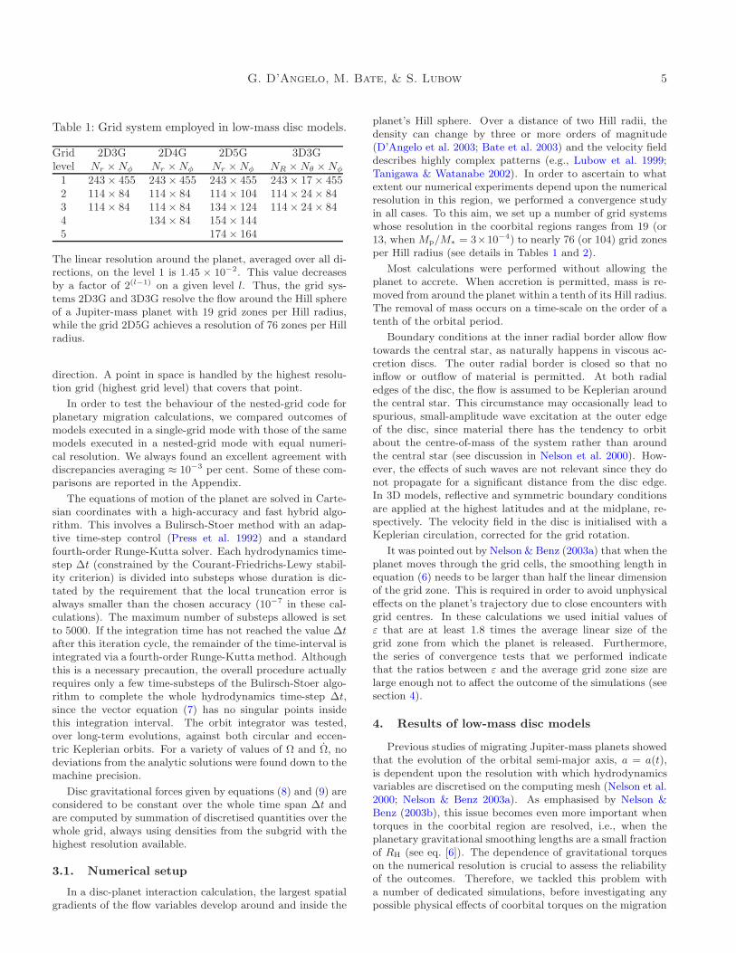
Table 1: Grid system employed in low-mass disc models.

Grid 2D3G 2D4G 2D5G 3D3Glevel Nr ×Nφ Nr ×Nφ Nr ×Nφ NR ×Nθ ×Nφ

1 243× 455 243× 455 243× 455 243× 17× 4552 114× 84 114× 84 114× 104 114× 24× 843 114× 84 114× 84 134× 124 114× 24× 844 134× 84 154× 1445 174× 164

The linear resolution around the planet, averaged over all di-rections, on the level 1 is 1.45 × 10−2. This value decreasesby a factor of 2(l−1) on a given level l. Thus, the grid sys-tems 2D3G and 3D3G resolve the flow around the Hill sphereof a Jupiter-mass planet with 19 grid zones per Hill radius,while the grid 2D5G achieves a resolution of 76 zones per Hillradius.

direction. A point in space is handled by the highest resolu-tion grid (highest grid level) that covers that point.

In order to test the behaviour of the nested-grid code forplanetary migration calculations, we compared outcomes ofmodels executed in a single-grid mode with those of the samemodels executed in a nested-grid mode with equal numeri-cal resolution. We always found an excellent agreement withdiscrepancies averaging ≈ 10−3 per cent. Some of these com-parisons are reported in the Appendix.

The equations of motion of the planet are solved in Carte-sian coordinates with a high-accuracy and fast hybrid algo-rithm. This involves a Bulirsch-Stoer method with an adap-tive time-step control (Press et al. 1992) and a standardfourth-order Runge-Kutta solver. Each hydrodynamics time-step ∆t (constrained by the Courant-Friedrichs-Lewy stabil-ity criterion) is divided into substeps whose duration is dic-tated by the requirement that the local truncation error isalways smaller than the chosen accuracy (10−7 in these cal-culations). The maximum number of substeps allowed is setto 5000. If the integration time has not reached the value ∆tafter this iteration cycle, the remainder of the time-interval isintegrated via a fourth-order Runge-Kutta method. Althoughthis is a necessary precaution, the overall procedure actuallyrequires only a few time-substeps of the Bulirsch-Stoer algo-rithm to complete the whole hydrodynamics time-step ∆t,since the vector equation (7) has no singular points insidethis integration interval. The orbit integrator was tested,over long-term evolutions, against both circular and eccen-tric Keplerian orbits. For a variety of values of Ω and Ω, nodeviations from the analytic solutions were found down to themachine precision.

Disc gravitational forces given by equations (8) and (9) areconsidered to be constant over the whole time span ∆t andare computed by summation of discretised quantities over thewhole grid, always using densities from the subgrid with thehighest resolution available.

3.1. Numerical setup

In a disc-planet interaction calculation, the largest spatialgradients of the flow variables develop around and inside the

planet’s Hill sphere. Over a distance of two Hill radii, thedensity can change by three or more orders of magnitude(D’Angelo et al. 2003; Bate et al. 2003) and the velocity fielddescribes highly complex patterns (e.g., Lubow et al. 1999;Tanigawa & Watanabe 2002). In order to ascertain to whatextent our numerical experiments depend upon the numericalresolution in this region, we performed a convergence studyin all cases. To this aim, we set up a number of grid systemswhose resolution in the coorbital regions ranges from 19 (or13, when Mp/M∗ = 3×10−4) to nearly 76 (or 104) grid zonesper Hill radius (see details in Tables 1 and 2).

Most calculations were performed without allowing theplanet to accrete. When accretion is permitted, mass is re-moved from around the planet within a tenth of its Hill radius.The removal of mass occurs on a time-scale on the order of atenth of the orbital period.

Boundary conditions at the inner radial border allow flowtowards the central star, as naturally happens in viscous ac-cretion discs. The outer radial border is closed so that noinflow or outflow of material is permitted. At both radialedges of the disc, the flow is assumed to be Keplerian aroundthe central star. This circumstance may occasionally lead tospurious, small-amplitude wave excitation at the outer edgeof the disc, since material there has the tendency to orbitabout the centre-of-mass of the system rather than aroundthe central star (see discussion in Nelson et al. 2000). How-ever, the effects of such waves are not relevant since they donot propagate for a significant distance from the disc edge.In 3D models, reflective and symmetric boundary conditionsare applied at the highest latitudes and at the midplane, re-spectively. The velocity field in the disc is initialised with aKeplerian circulation, corrected for the grid rotation.

It was pointed out by Nelson & Benz (2003a) that when theplanet moves through the grid cells, the smoothing length inequation (6) needs to be larger than half the linear dimensionof the grid zone. This is required in order to avoid unphysicaleffects on the planet’s trajectory due to close encounters withgrid centres. In these calculations we used initial values ofε that are at least 1.8 times the average linear size of thegrid zone from which the planet is released. Furthermore,the series of convergence tests that we performed indicatethat the ratios between ε and the average grid zone size arelarge enough not to affect the outcome of the simulations (seesection 4).

4. Results of low-mass disc models

Previous studies of migrating Jupiter-mass planets showedthat the evolution of the orbital semi-major axis, a = a(t),is dependent upon the resolution with which hydrodynamicsvariables are discretised on the computing mesh (Nelson et al.2000; Nelson & Benz 2003a). As emphasised by Nelson &Benz (2003b), this issue becomes even more important whentorques in the coorbital region are resolved, i.e., when theplanetary gravitational smoothing lengths are a small fractionof RH (see eq. [6]). The dependence of gravitational torqueson the numerical resolution is crucial to assess the reliabilityof the outcomes. Therefore, we tackled this problem witha number of dedicated simulations, before investigating anypossible physical effects of coorbital torques on the migration


Table 2: Grid system utilised in high-mass disc models.

Grid 2D1Gb 2D3Gb 2D4Gb 2D5Gb 2D6Gb 3D3Gblevel Nr ×Nφ Nr ×Nφ Nr ×Nφ Nr ×Nφ Nr ×Nφ NR ×Nθ ×Nφ

1 147× 455 147× 455 147× 455 147× 455 147× 455 147× 17× 4552 114× 84 114× 84 114× 84 134× 104 84× 24× 843 114× 84 114× 84 114× 84 134× 104 84× 24× 844 114× 84 134× 84 164× 1045 164× 104 194× 1246 324× 204

The average linear resolution around the planet on the level l is 1.43× 10−2/2(l−1). Hence, thegrid systems 2D3Gb and 3D3Gb resolve the flow around the Roche lobe of a 0.3MJ planet with13 grid zones per Hill radius while the grid 2D6Gb achieves a resolution of more than 100 zonesper Hill radius. We used the single-level grid system, 2D1Gb, only for purposes of comparisonwith the calculations reported in MP03,

of giant planets.

4.1. A convergence study

Convergence tests were carried out on each of the low-massdisc models described in Section 2.4.1. The resolution wasprogressively increased by employing the grid systems 2D3G,2D4G, and 2D5G (see Table 1). The last two grid systems,compared to the first, provide a linear resolution gain of afactor 2 and 4, respectively. For comparison purposes, we set

Fig. 1.— Global surface density around a Mp = 1MJ planetorbiting in a low-mass disk (see section 2.4.1). The density isshown after 370 orbits, when the planet has migrated for 70orbits. In the linear grey-scale, at 5.2AU, Σ = 10−4 corre-sponds to 32.9 g cm−2.

the release time to trls = 100 orbits, except for the simulationsconcerning the accreting model that have trls = 300 orbits.The overall surface density from one of such calculations isdisplayed in Figure 1.

Figure 2 shows that we achieved numerical convergencein all cases, with either accreting or non-accreting planetsand with different values of ε. In some panels, the out-

Fig. 3.— Surface density profile along the azimuthal position(φ = φp) of a Mp = 1MJ planet, after 100 orbital periods,orbiting in a low-mass disc. Different line types indicate mod-els with different values of the gravitational potential soften-ing: ε = 0.1RH (solid line); ε = 0.2RH (short-dash line);ε = 0.4RH (dash-dot line); accreting planet (long-dash line).If a0 = 5.2AU and M∗ = 1M⊙, Σ = 10−4 corresponds to32.9 g cm−2.


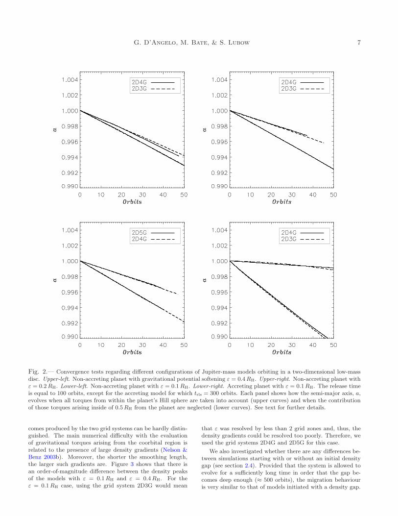
Fig. 2.— Convergence tests regarding different configurations of Jupiter-mass models orbiting in a two-dimensional low-massdisc. Upper-left. Non-accreting planet with gravitational potential softening ε = 0.4RH. Upper-right. Non-accreting planet withε = 0.2RH. Lower-left. Non-accreting planet with ε = 0.1RH. Lower-right. Accreting planet with ε = 0.1RH. The release timeis equal to 100 orbits, except for the accreting model for which trls = 300 orbits. Each panel shows how the semi-major axis, a,evolves when all torques from within the planet’s Hill sphere are taken into account (upper curves) and when the contributionof those torques arising inside of 0.5RH from the planet are neglected (lower curves). See text for further details.

comes produced by the two grid systems can be hardly distin-guished. The main numerical difficulty with the evaluationof gravitational torques arising from the coorbital region isrelated to the presence of large density gradients (Nelson &Benz 2003b). Moreover, the shorter the smoothing length,the larger such gradients are. Figure 3 shows that there isan order-of-magnitude difference between the density peaksof the models with ε = 0.1RH and ε = 0.4RH. For theε = 0.1RH case, using the grid system 2D3G would mean

that ε was resolved by less than 2 grid zones and, thus, thedensity gradients could be resolved too poorly. Therefore, weused the grid systems 2D4G and 2D5G for this case.

We also investigated whether there are any differences be-tween simulations starting with or without an initial densitygap (see section 2.4). Provided that the system is allowed toevolve for a sufficiently long time in order that the gap be-comes deep enough (≈ 500 orbits), the migration behaviouris very similar to that of models initiated with a density gap.


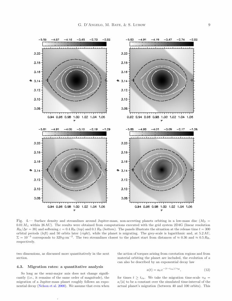
Two sets of lines are displayed in each panel of Figure 2.These are intended to address the lingering question of theimportance of torques exerted by matter residing deep insidethe planet’s Hill sphere (D’Angelo et al. 2003; Bate et al.2003). Thus, two configurations were simulated, differing onlyin whether or not torques within a radius βRH from the planetare included in the calculation of the gravitational force inequations (8) and (9). In one configuration, all torques aretaken into account (i.e., β = 0). In the second configuration,the simulations were repeated neglecting the contribution ofmaterial lying inside the inner half of the Hill sphere (i.e., β =0.5). The choice β = 0.5 was made to avoid the region wherethe density gradient is largest (see Fig. 3) and which mostlycontains material orbiting the planet before it is released (seeFig. 4).

The streamlines in Figure 4 are constructed by integrat-ing the velocity field (ur, uφ) at an instant in time. Strictlyspeaking, this procedure is in error for a migrating planet(right panels), as it moves during the interval of integration.But provided the planet moves only a small fraction of its Hillsphere over the integration time, the streamlines obtainedare reasonably accurate. This condition is satisfied for thestreamlines plotted in this Figure. It is of course incorrectto ignore torques from within the Hill sphere since materialcan move into or out of it (see Fig. 3) and the angular mo-mentum associated with this mass flux is lost instead of beingtransferred to the planet’s orbit. Therefore, migration ratesobtained from configurations with β > 0 are not fully consis-tent from a physical standpoint, unless one can assure thatthe neglected material is constantly and not temporarily or-biting the planet.

In all cases we considered, the β = 0 calculations resultedin slower migration and, thus, these results appear as theupper curves in each panel of Figure 2. We note that evenwhen torques coming from material within the Hill sphereare included, numerical convergence is still achieved. Thislast point turns out to be crucial when high-mass discs areconsidered (see section 5).

4.2. Three-dimensional simulations

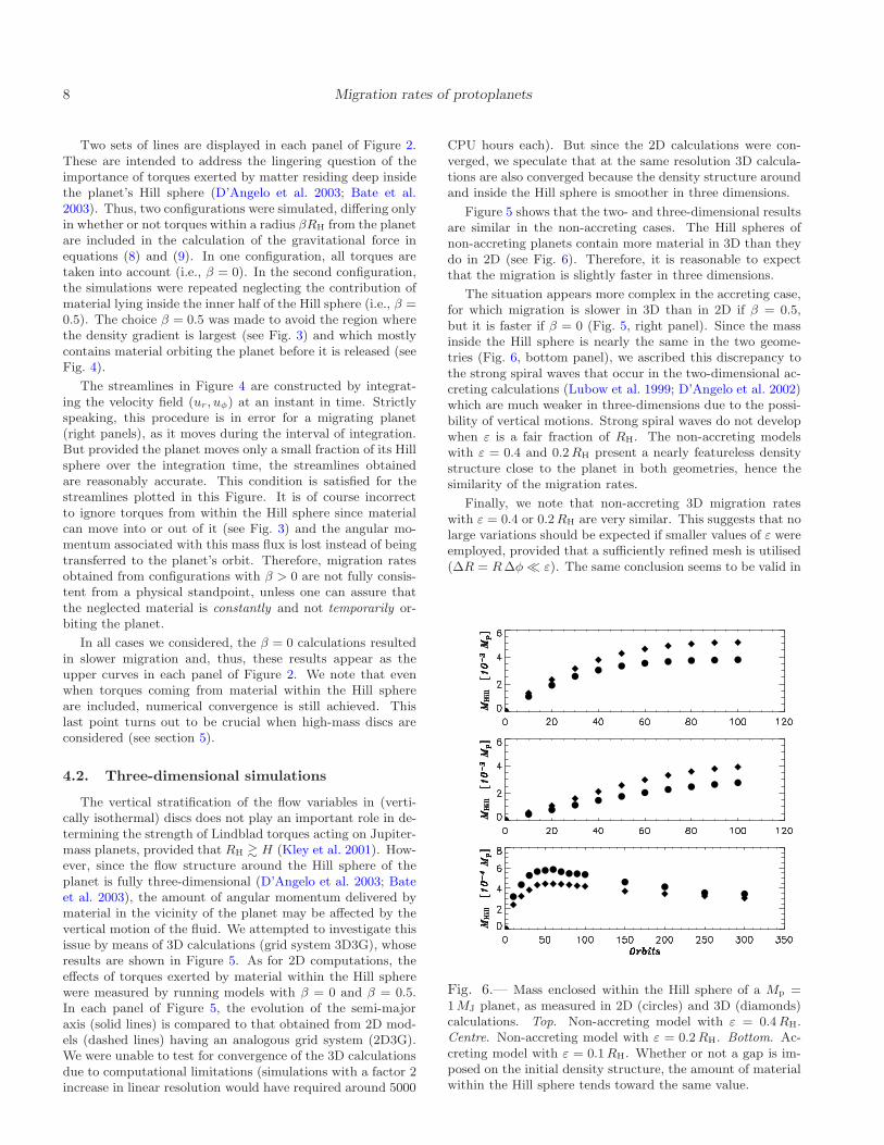
The vertical stratification of the flow variables in (verti-cally isothermal) discs does not play an important role in de-termining the strength of Lindblad torques acting on Jupiter-mass planets, provided that RH & H (Kley et al. 2001). How-ever, since the flow structure around the Hill sphere of theplanet is fully three-dimensional (D’Angelo et al. 2003; Bateet al. 2003), the amount of angular momentum delivered bymaterial in the vicinity of the planet may be affected by thevertical motion of the fluid. We attempted to investigate thisissue by means of 3D calculations (grid system 3D3G), whoseresults are shown in Figure 5. As for 2D computations, theeffects of torques exerted by material within the Hill spherewere measured by running models with β = 0 and β = 0.5.In each panel of Figure 5, the evolution of the semi-majoraxis (solid lines) is compared to that obtained from 2D mod-els (dashed lines) having an analogous grid system (2D3G).We were unable to test for convergence of the 3D calculationsdue to computational limitations (simulations with a factor 2increase in linear resolution would have required around 5000

CPU hours each). But since the 2D calculations were con-verged, we speculate that at the same resolution 3D calcula-tions are also converged because the density structure aroundand inside the Hill sphere is smoother in three dimensions.

Figure 5 shows that the two- and three-dimensional resultsare similar in the non-accreting cases. The Hill spheres ofnon-accreting planets contain more material in 3D than theydo in 2D (see Fig. 6). Therefore, it is reasonable to expectthat the migration is slightly faster in three dimensions.

The situation appears more complex in the accreting case,for which migration is slower in 3D than in 2D if β = 0.5,but it is faster if β = 0 (Fig. 5, right panel). Since the massinside the Hill sphere is nearly the same in the two geome-tries (Fig. 6, bottom panel), we ascribed this discrepancy tothe strong spiral waves that occur in the two-dimensional ac-creting calculations (Lubow et al. 1999; D’Angelo et al. 2002)which are much weaker in three-dimensions due to the possi-bility of vertical motions. Strong spiral waves do not developwhen ε is a fair fraction of RH. The non-accreting modelswith ε = 0.4 and 0.2RH present a nearly featureless densitystructure close to the planet in both geometries, hence thesimilarity of the migration rates.

Finally, we note that non-accreting 3D migration rateswith ε = 0.4 or 0.2RH are very similar. This suggests that nolarge variations should be expected if smaller values of ε wereemployed, provided that a sufficiently refined mesh is utilised(∆R = R∆φ ≪ ε). The same conclusion seems to be valid in

Fig. 6.— Mass enclosed within the Hill sphere of a Mp =1MJ planet, as measured in 2D (circles) and 3D (diamonds)calculations. Top. Non-accreting model with ε = 0.4RH.Centre. Non-accreting model with ε = 0.2RH. Bottom. Ac-creting model with ε = 0.1RH. Whether or not a gap is im-posed on the initial density structure, the amount of materialwithin the Hill sphere tends toward the same value.


Fig. 4.— Surface density and streamlines around Jupiter-mass, non-accreting planets orbiting in a low-mass disc (MD =0.01M⊙ within 26AU). The results were obtained from computations executed with the grid system 2D4G (linear resolutionRH/∆r = 38) and softening ε = 0.4RH (top) and 0.1RH (bottom). The panels illustrate the situation at the release time t = 300orbital periods (left) and 50 orbits later (right), while the planet is migrating. The grey-scale is logarithmic and, at 5.2AU,Σ = 10−3 corresponds to 329 g cm−2. The two streamlines closest to the planet start from distances of ≈ 0.36 and ≈ 0.5RH,respectively.

two dimensions, as discussed more quantitatively in the nextsection.

4.3. Migration rates: a quantitative analysis

So long as the semi-major axis does not change signifi-cantly (i.e., it remains of the same order of magnitude), themigration of a Jupiter-mass planet roughly follows an expo-nential decay (Nelson et al. 2000). We assume that even when

the action of torques arising from corotation regions and frommaterial orbiting the planet are included, the evolution of acan also be described by an exponential decay law

a(t) = a0 e−(t−trls)/τM , (12)

for times t ≥ trls. We take the migration time-scale τM =a/|a| to be a constant over the simulated time-interval of theactual planet’s migration (between 40 and 100 orbits). This


Fig. 5.— Three-dimensional simulations of Jupiter-mass models (grid system 3D3G) orbiting in a low-mass disc, comparedto analogous two-dimensional models (grid system 2D3G). Left. Non-accreting planet with gravitational potential softeningε = 0.4RH. Centre. Non-accreting planet with ε = 0.2RH. Right. Accreting planet with ε = 0.1RH. The release time is equalto 100 orbits for the non-accreting models and 300 orbits for the accreting models. In each panel, the slower migration occurswith the configuration executed with β = 0, whereas the faster migration occurs with the configuration run with β = 0.5.

simple parameterisation of a = a(t) is very useful becauseτM can be directly connected to the acting torques. In fact,if the orbit eccentricity is negligible then the conservation ofthe orbital angular momentum leads to the relation

a =2T ·Ω

Mp aΩ2, (13)

in which the vector T denotes the total external torque. Thisexpression is commonly used to evaluate a from the verticalcomponent of T (which we simply indicate as T ), when aplanet moves on a static orbit (i.e., it is not allowed to mi-grate).

We obtained estimates of τM for all of the 2D models (gridsystem 2D4G) by performing a linear least-mean-squared fitof the relation ln (a/a0) = −(t − trls)/τM. The results arelisted in the second and third columns of Table 3, labelledas “moving” migration time-scale. The relative error on eachestimate is at most 10−3 and only for this reason τM is givenwith three significant digits. Discrepancies between estimatescomputed from 2D and 3D non-accreting models are below∼ 10 per cent. Since the accreting models present a moresignificant discrepancy, τM is also reported for the simulationsin three dimensions.

Including the effect of matter orbiting the planet tends toslow down its inward drifting motion, regardless of the em-ployed disc geometry, as clearly indicated in Figure 5. Thecomparison between the β = 0 and β = 0.5 migration time-scales shows that the torque from this material can be compa-rable to that from corotation and Lindblad resonances. Thetotal (positive) torque produced inside the inner half of theHill sphere is

THS = T − TLC ∝1

τM[β = 0]−

1

τM[β = 0.5], (14)

whereas the magnitude of the total (negative) torque ex-erted from the rest of the disc (i.e., Lindblad and corotation

torques), |TLC|, is proportional to 1/τM[β = 0.5]. Hence, theratio between the two contributions is

THS

|TLC|= 1−

τM[β = 0.5]

τM[β = 0]. (15)

Entries in the second and third columns of Table 3 indicatethat in the model with softening ε = 0.4RH the material closeto the planet accounts for a relatively small contribution (22per cent). However, shorter smoothing lengths dramaticallyincrease the torque ratio, which becomes greater than 60 percent in the non-accreting models with ε = 0.2RH and 0.1RH.A similar ratio between torques is obtained in the 3D accret-ing model.

These migration time-scales can be compared with theType I (no gap, resonant) time-scale of about 4 × 102 or-bits in 2D and 6× 102 orbits in 3D (Tanaka et al. 2002) andthe Type II (viscous) time-scale 2 a2/(3 ν) ≃ 104 orbits.

Note that the 2D migration rates tend to converge as ε isdecreased. In particular, the migration rates for ε = 0.2RH

and 0.1RH differ by less than 10 per cent.

4.4. Comparison of migration rates of static and

migrating planets: the Jupiter-mass case

We examined whether the torque exerted on the planetby the disc material is influenced by the radial motion of theplanet. As discussed in Section 1, the motion of the planetmight be able to affect the coorbital torques and thereforethe migration rate. In order to test this hypothesis, we com-puted the total torque acting on the planet during the lastten orbital periods before it was released. This was done forboth β = 0 and β = 0.5 configurations. Since no angularmomentum is actually extracted from or added to the plan-etary orbit, which thus remains static, we shall refer to suchtorques as static torques. The migration time-scales listed inthe two right-most columns of Table 3 were obtained from theaverage static torques by using equation (13). In Table 3 we


compared these “static” migration time-scales, τSM, with the

migration time-scales, τM, measured from the moving planetcalculations. In all cases, there is close agreement between thestatic and moving migration time-scales. These results showthat under these circumstances of disc and planetary masses,there is no strong dependence of the torques on whether plan-ets are on fixed orbits or allowed to migrate.

5. Results of high-mass disc models

The Type II migration rate depends only on the viscoustime-scale of the disc near the location of the planet and is in-dependent of the disc density, provided that the gap is devoidof material. Yet gaps are generally not completely cleared andthe Type II time-scale prediction does not take into consider-ation the angular momentum exchanged between the planetand the “gap” material. Some of this material travels onhorse-shoe orbits, while other material circulates within theplanet’s Hill sphere. The angular momentum delivered in ei-ther case may play a major role in planetary migration (see,e.g., Masset 2001) and it is proportional to the local massdensity. In fact, MP03 recently claimed that there exists acritical mass (when the material around the planet is moremassive than the planet), beyond which a runaway migrationprocess sets in.

We ran simulations of Saturn-like bodies (Mp = 0.3MJ)embedded in a disc as massive as 24MJ inside 13AU. Theannular region within 2RH from the planet is initially 7.5 asmassive as the planet. Nonetheless, the aspect ratio is smallenough (H/r = 0.03) so the thermal condition for gap for-mation, Mp/M∗ > 3 (H/r)3 (e.g., Lin & Papaloizou 1993),is fulfilled and therefore the migration might be within theType II regime, although the gap is not completely clearedas can be seen in Figure 7. In these cases, with massive discs

Table 3: Comparison of static and moving migrationtime-scales for a Jupiter-mass planet in a low-mass disc.

Moving Staticε

β = 0 β = 0.5 β = 0 β = 0.5

0.4RH 9.94× 103 7.75× 103 1.0× 104 7.8× 103

0.2RH 1.76× 104 6.34× 103 1.8× 104 6.2× 103

0.1RH 1.51× 104 5.71× 103 1.8× 104 5.7× 103

0.1RH† 5.97× 104 4.86× 103 4.8× 104 4.2× 103

0.1RH‡ 1.54× 104 5.77× 103 1.5× 104 5.4× 103

† 2D accreting model. ‡ 3D accreting model.

The migration time-scales labelled as “moving” refer to thetime-scale, τM, in equation (12) and were computed as ex-plained in Section 4.3. They are expressed in units of initialorbital periods, i.e., 11.9 years if a0 = 5.2AU. One-standarddeviation uncertainties for these estimates range from 1 to 10orbits. See Section 4.1 for an explanation of configurationsβ = 0 and β = 0.5. Migration time-scales labelled as “static”were determined from equation (13) by employing torques av-eraged over the last ten orbits before the release time. Com-putations were executed with the grid system 2D4G.

and small aspect ratios, very large density gradients developinside the Hill sphere. Therefore, it is especially important toinvestigate the dependence of the results on numerical resolu-tion. We achieved convergence for the flow outside of the Hillsphere by using numerical resolutions of order 13 grid zonesper Hill radius. However, in order to accurately determinethe contributions to the migration rate from material insidethe Hill sphere, resolutions higher than 52 grid zones per Hillradius are necessary.

5.1. Convergence tests

As mentioned in Section 2.4.2, the model setup and thedisc parameters were chosen to match as closely as possiblethose in MP03. The smoothing length was 60 per cent of thelocal disc thickness, H , (i.e., ε = 0.3878RH), the planet wasnon-accreting, and trls = 477 orbits. We performed a calcu-lation using a single-level grid (2D1Gb, see Table 2) aimedat reproducing the resolution used by MP03 (∆r/RH ≃ 0.3and ∆r/ε ≃ 0.8). We then performed a convergence test us-ing different numerical resolutions, as provided by the gridsystems 2D3Gb, 2D4Gb, and 2D5Gb (see Table 2). An addi-tional convergence test, involving the grid system 2D6Gb, isdiscussed in Section 5.1.1.

The left panel of Figure 8 shows the outcomes of the testsfor the evolution of the semi-major axis concerning the con-figuration with β = 0. The dot-dash line in this panel rep-resents the result from the single-grid computation 2D1Gb,

Fig. 7.— Global surface density around aMp = 0.3MJ (non-accreting) planet orbiting in a 0.024M⊙ disk. The density isdisplayed at t = 550 orbits, when the planet has migrated forabout 70 orbits. The grey-scale is logarithmic and 10−3 cor-responds to 329 g cm−2, at 5.2AU. The average gap densityis 2.5× 10−4 or 82 g cm−2.


Fig. 8.— Computations of a Saturn-mass planet orbiting in a high-mass disc: convergence tests. The gravitational potentialsoftening, ε, is 60 per cent of the local disc scale-height. The release time is equal to 477 orbits. The left panel shows theevolution of a when all torques are taken into account (i.e., β = 0). The right panel shows how the evolution of the semi-majoraxis proceeds when the contribution of those torques arising from inside the Hill sphere (i.e., β = 1.0) are neglected . Thedot-dash line (labelled as 2D1Gb) refers to a calculation executed with the same numerical resolution as in MP03.

which should be compared to the model labelled as S8 in Fig-ure 2 of MP03. Given the remarkable agreement between ourand their outcome, we are confident that we reproduced thesame physical and numerical conditions for runaway migra-tion. Yet, computations repeated with finer and finer res-olutions gave smaller and smaller migration rates which, asdisplayed in Figure 8 (left panel), failed to converge. The gainin linear resolution achieved (over the single-grid simulation)with the employed grid systems ranges from 4 (2D3Gb) to16 (2D5Gb). In the highest resolution models, there are 52grid zones per Hill radius. Comparing the short-dash anddot-dash curves in left panel of Figure 8, one realises thatthe average migration speed obtained over the first 25 or-bits with the grid system 2D3Gb is only half (in physicalunits, 〈a〉 ≈ −5 × 10−3 AUyr−1) of that in MP03. Calcu-lations executed with the grid systems 2D4Gb and 2D5Gbgive even lower migration speeds of 〈a〉 ≃ −5 × 10−4 and−1.4× 10−4 AUyr−1, respectively.

While there is a factor of 10 decrease in disc torques actingon the planet in going from grid systems 2D3Gb to 2D4Gb,this factor reduces to 3.6 when the two most refined gridsystems are considered. Yet, from the behaviour of semi-major axis evolution shown in the left panel of Figure 8, wecannot determine whether it is converging. To assess thispoint we employed the grid system 2D6Gb (see section 5.1.1)which indicates that the solid line in Figure 8 is basically aconverged evolution.

The right panel in Figure 8 shows the semi-major axisevolution from the same calculations as in the left panel butexecuted with β = 1.0, i.e., excluded torques arising inside theplanet’s Hill sphere. As before, this choice of β was made to

Fig. 9.— Mass enclosed within the Hill sphere of a Mp =0.3MJ planet, as measured from simulations with increasingresolutions: single-level grid 2D1Gb (asterisks); grid system2D3Gb (diamonds); grid system 2D4Gb (squares); grid sys-tem 2D5Gb (circles).


exclude the region around the planet with largest density gra-dients as well as largest torque densities. Clearly, numericalconvergence was readily achieved with this configuration. Themigration time-scale, obtained from a least-mean-squared fitto the data (see section 4.3), is τM = 493 orbits. Furthermore,outcomes of simulations executed with β = 0.75 attained con-vergence at almost the same rate of migration as with β = 1.0.Therefore, we conclude that the material close to the planetmust be held responsible for the non-convergence of the β = 0configuration in the left panel of Figure 8. That is, the torquearising from within the Hill sphere converges very slowly withincreasing resolution. Despite the fact that the amount of ma-terial inside the planet’s Hill sphere increases as the grid res-olution is raised (see Fig. 9), the resulting migration rates ornet torques are actually smaller. Figure 10 shows the surfacedensity near the planet at an advanced time, shortly before itis allowed to migrate. We note that the mass near the planetseems to be converging at the highest resolutions, but conver-gence is not yet formally achieved. This Figure also impliesthat most of the material is piled up very close to the planet.We measured that 80 per cent of the mass contained insidethe Hill sphere is concentrated within a distance of 0.2RH

from the planet.

The mass build up within the Hill sphere appears to sug-gest that disc self-gravity may be dynamically important.However, this may not actually be the case. A simple cal-culation of a viscous disc that accretes at the typical rates of

Fig. 10.— Surface density profile at the azimuthal posi-tion of a planet with Mp/M∗ = 3 × 10−4, after 450 orbitalperiods (the planet starts migrating at trls = 477 orbits),orbiting within a high-mass disc. Different line types re-fer to computations performed with different grid systems:2D5Gb (solid line); 2D4Gb (long-dash line); 2D3Gb (short-dash line). If a0 = 5.2AU and M∗ = 1M⊙, Σ = 10−2 is equalto 3.29× 103 g cm−2.

10−8 M⊙ per year suggests that it is likely not self-gravitating(the value of the Toomre parameter Q is much greater thanunity for the parameters in this paper). In the simulationspresented here, the mass build up is concentrated in a re-gion of order the smoothing length (see Fig. 10). Within thatradius, further inward viscous accretion is artificially slow be-cause the gravitational potential of the planet tends to enforcerigid rotation (see second term in eq. [6]). In addition, theboundary condition of no accretion on the planet prevents theaccumulated gas from being removed from the simulation. Assuch, much of the gas accumulated within a smoothing lengthrepresents material that is incorporated by the planet, ratherthan residing in the disc.

Although the configuration with β = 1.0 provides nu-merically converged migration rates, one has to be wary oftheir physical meaning. Figure 11 illustrates that before theplanet is released (top-left panel) material on horse-shoe or-bits passes through the Roche lobe as close to the planet as≈ 0.5RH. Yet, if the planet starts rapidly migrating thispicture is bound to change. The top-right panel shows asnapshot after 20 orbits from the release time, as the planetradially moves at a speed a ≃ −1.5 × 10−4 AUyr−1 (con-figuration β = 1.0 and grid system 2D5Gb). The situationappears less symmetric than before the release and the flowstructure within the Hill sphere has been altered by the rapidplanetary motion. As a reference, we also show in the bottompanel what happens when all torques are consistently takeninto account (β = 0). We calculated the torques arising fromthe Hill sphere in the situation depicted in the top-right paneland we found that they are three times as large (and morepositive) as those exerted, at the same time, in the configura-tion β = 0 (bottom panel). This difference may indicate thatthe faster motion in the β = 1 case has artificially changedthe density distribution inside the Hill sphere and thus thecirculation in the coorbital region.

The reason for the very fast migration rate, measured atthe lowest resolution (single-level grid 2D1Gb), can be un-derstood by examining the two dimensional linear map of thetorque density magnitude in the left panel of Figure 12. Theplot describes the situation after 19 orbits from the planet’srelease, when it is migrating inwards at an average rate ofroughly 10−2 AUyr−1. The map clearly shows how the poorresolution (the grid zone size is indicated by the shaded pix-els) cannot properly handle the large torque gradients withinthe Hill sphere and produces a very large differential torque.This resolution effect led to the vastly different migrationtime-scales between the lowest and highest curves in the leftpanel of Figure 8. A cut of the torque density magnitude,through the planet’s radial position, is shown in the rightpanel of Figure 12 for both the computation executed withthe grid 2D1Gb (solid line) and that executed with the high-resolution grid system 2D5Gb (dashed line). The dashed-lineprofile was rescaled so that the maximum values were similarto those of the solid-line profile. The filled circles representthe actual data. The low-resolution torque density is highlyasymmetric. The two maxima alone exert a negative torquethat would result in a migration time-scale of 80 orbits. Thelarge mismatch between the torque density extrema is not ob-served in high-resolution model, in which their opposite signcontributions nearly cancel each other.


Fig. 11.— Surface density and streamlines around aMp = 0.3MJ, non-accreting planet orbiting in a high-mass disc (MD = 0.024M⊙ within 13AU). The dashedline indicates the Roche lobe and the crosses mark theposition of the L1 and L2 Lagrange points. The top-left panel refers to the time t = 450 orbital periods(i.e., before it is released) whereas the top-right paneldisplays the situation at t = 497 orbits with the con-figuration β = 1.0 (its instantaneous radial speed isa ≃ −1.5× 10−4 AUyr−1). The bottom panel refers tothe same time but when all torques are taken into ac-count (i.e., β = 0). The grey-scale is logarithmic and, at5.2AU, 10−3 corresponds to 329 g cm−2. These resultswere obtained from computations executed with the gridsystem 2D5Gb (linear resolution ∆r/RH ≃ 2 × 10−2).As in Figure 4, the streamlines in the bottom paneldo not account for the planet’s motion because of thesmall a. A more strict procedure was instead employedto calculate the streamlines in the top-right panel. Inthis case we integrated the velocity field (ur − a, uφ),where a is the instantaneous radial speed of the planet.

The differences between the two highest resolution calcu-lations discussed here are less evident and require some dis-cussion. Two-dimensional logarithmic maps of the magni-tude of the torque density for such models are shown in thetop panels of Figure 13. They were obtained from the com-putations with the grid systems 2D4Gb (left) and 2D5Gb(right). Both maps describe the situation 60 orbits after theplanet’s release. The torque density is positive on the sideleading the planet, φ > φp, and negative on the oppositeside (φ < φp). As clearly indicated in the Figure, the torquedensity within the inner half of the Hill sphere is orders ofmagnitudes larger than it is anywhere else in the surroundingregion and, therefore, in the whole disc. This is the reasonwhy the migration speed is so susceptible to the torques ex-erted within the planet’s Hill lobe. Any mismatch between

the positive (φ > φp) and negative (φ > φp) contributionscan produce a very large net (either positive or negative)torque acting on the planet. From the top panels in Fig-ure 13, the torque density magnitude appears rather symmet-ric with respect to the direction φ = φp. This is clear fromthe bottom-left panel, where cuts through the planet’s radialposition are compared for the two grid systems. The solidline corresponds to the more resolved model. Nevertheless,the results shown in the bottom-left panel of Figure 8 implythat the torque exerted by the Hill sphere is more positive(i.e., greater than zero and larger) in the higher resolutionmodel (grid system 2D5Gb) than it is in the lower resolutionone (grid system 2D4Gb). Indeed, this effect is highlightedby the ratio between the two torque density cuts (solid todashed profile, that is higher to lower resolution results) re-


Fig. 12.— Left. Absolute value of the torque density (linear scale) close to a planet with Mp/M∗ = 3× 10−4 and orbiting in ahigh-mass disc. The dashed line indicates the Roche lobe and the crosses mark the L1 and L2 Lagrange points. This calculationwas executed with the single-level grid 2D1Gb (∆r ≃ 0.3RH). Shaded pixels represent the actual size of the grid zones. Thetorque distribution is illustrated at t = 496 orbital periods while the planet is migrating at an average rate 〈a〉 ≈ −10−2 AUyr−1.The torque density is negative when φ < φp = π and positive when φ > φp. It is evident that at such low resolution there is anunbalanced inward torque that is not observed in higher resolution calculations (see top panels of Fig. 13). Right. The solid lineshows the profile of the absolute value of the torque density (shown in the left panel) through the radial position of the planet.The filled circles indicate the positions of the data. The dashed line refers to an analogous profile from the highest resolutioncalculation (grid system 2D5Gb), which was rescaled so that its maximum value was 1.3× 10−6.

ported in the bottom-right panel of Figure 13. The importantthing to note is that the curve is asymmetric, with respect tothe direction φ = φp, towards the the outer parts of the Hillsphere |φ− φp| > 0.02 ≃ 0.4RH/a. This means that the mis-match between the positive (φ > φp) and negative (φ < φp)torques arising from the region |φ − φp| > 0.02 produces anet positive torque that is greater in the higher resolutionmodel than it is in the lower resolution model. Most of theasymmetry, and therefore the discrepancy between the twocomputations, must be confined to the region enclosed be-tween roughly 0.4RH and 0.75RH from the planet becauseconvergence tests executed with the configuration β = 0.75gave the same migration behaviour for the two models.

We also performed 3D simulations, using the grid system3D3Gb (see Table 2), yet no appreciable differences from 2Dcalculations executed with the grid system 2D3Gb were ob-served. This was easily predictable, given the large smoothinglength adopted in these models and the very small the discthickness.

5.1.1. A converged migration rate

In order to evaluate how close to convergence the orbitalevolution given by the grid system 2D5Gb is (see Fig. 8, leftpanel), we made a final attempt and ran a model with thegrid system 2D6Gb (see Table 2), which resolves the Hill ra-dius with about 104 grid zones. However, we could not runa complete model as those in Section 5.1. In fact, evolving a

model for about 550 orbits with such a grid system would haverequired around 8000 CPU hours. We only had the compu-tational resources to run this particular model for about 292orbital periods. Therefore we set the release time to trls = 277orbits and let the planet migrate for about 15 orbits.

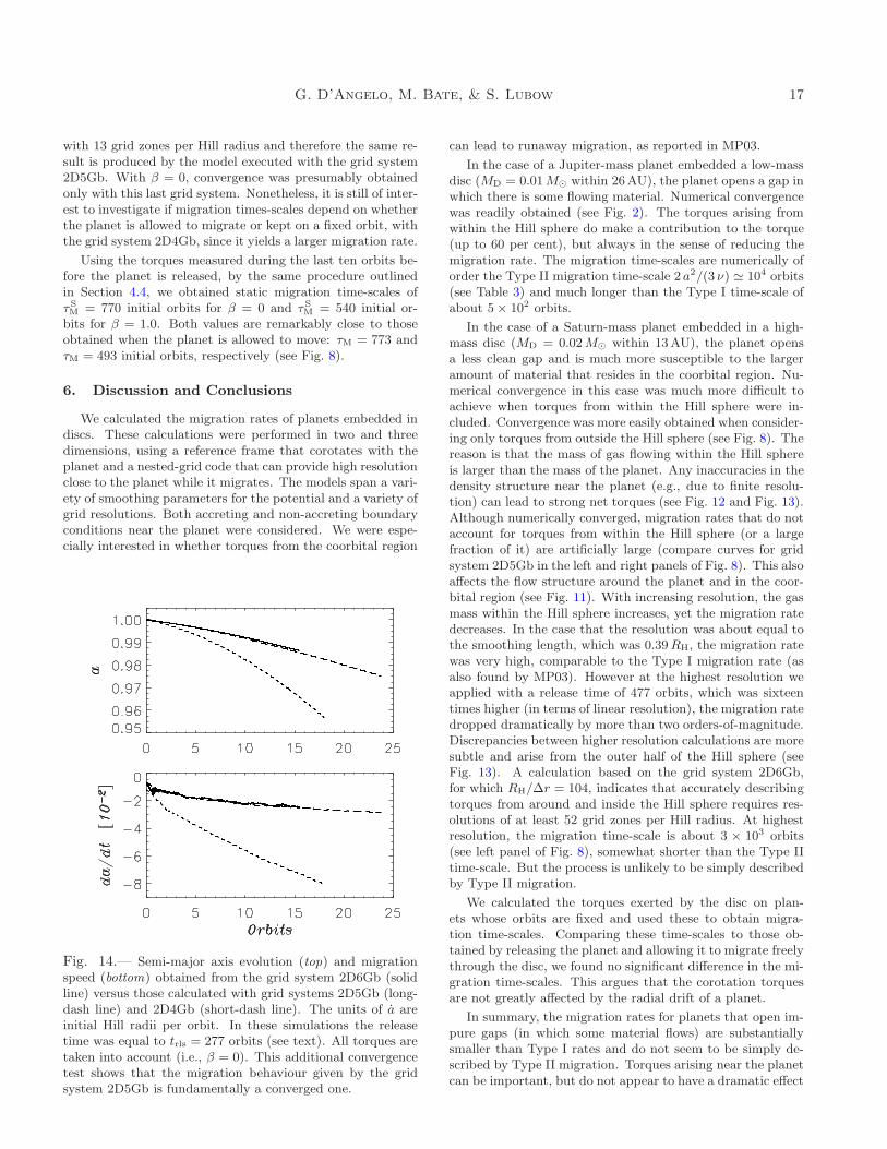
To carry out a consistent comparison, we performed cal-culations with the grid systems 2D4Gb and 2D5Gb imposingthe same release time. The results are shown in Figure 14.Despite the short time over which the planet actually mi-grated, the highest resolution model (solid lines) providedevolutions of both a (top panel) and a (bottom panel) thatare in very good agreement with those computed with the gridsystem 2D5Gb (long-dash lines). This implies that the ratesof migration obtained with the latter grid system (2D5Gb)can be considered as converged rates. This also indicatesthat in order to accurately compute torques from within andaround the Hill sphere, in a configuration as described in Sec-tion 2.4.2, linear resolutions on the order of 52 grid zones perHill radius are required.

It has to be emphasised that, while for Jupiter-mass plan-ets in low-mass discs torques were converged with respect toboth the numerical resolution and the smoothing length ofthe planet’s potential (see section 4), in the present case weonly examined convergence with respect to the numerical res-olution.


Fig. 13.— Top. Absolute value of the torque density (logarithmic scale) and contour lines around and inside the Hill sphere ofa planet with Mp/M∗ = 3× 10−4, orbiting in a high-mass disc. The snapshots are taken at t = 537 orbital periods, i.e., afterthe planet has migrated for 60 orbits. The left panel refers to the calculation executed with the grid system 2D4Gb while theright panel refers to that executed with the grid system 2D5Gb. The torque density is negative when φ < φp and positive whenφ > φp. Note that the torque density at the planet position is not exactly zero because the planet does not sit on the centre ofa mesh zone, where density torque is computed. Bottom. The left panel shows the cut of the torque density magnitude throughthe planet’s radial position for the models shown in the top panels. The solid line represents the outcome of the higher resolutionsimulation (2D5Gb) whereas the dashed line corresponds to the lower resolution simulation (2D4Gb). The ratio between thesetwo curves (higher to lower resolution calculation) is displayed in the right panel. The profile appears asymmetric (with respectto φ− φp = 0) only towards the outer regions |φ− φp| > 0.02 ≃ 0.4RH/a.

5.2. Comparison of migration rates of static and

migrating planets: the Saturn-mass case

We performed the same type of comparison, as done above,for the torques acting on a static and migrating planet. We

considered both the configurations β = 0 and β = 1.0. Theseresults were obtained from the calculation run with the gridsystem 2D4Gb (26 grid zones per Hill radius). Recall thatwith β = 1.0, complete numerical convergence was attained


with 13 grid zones per Hill radius and therefore the same re-sult is produced by the model executed with the grid system2D5Gb. With β = 0, convergence was presumably obtainedonly with this last grid system. Nonetheless, it is still of inter-est to investigate if migration times-scales depend on whetherthe planet is allowed to migrate or kept on a fixed orbit, withthe grid system 2D4Gb, since it yields a larger migration rate.

Using the torques measured during the last ten orbits be-fore the planet is released, by the same procedure outlinedin Section 4.4, we obtained static migration time-scales ofτSM = 770 initial orbits for β = 0 and τS

M = 540 initial or-bits for β = 1.0. Both values are remarkably close to thoseobtained when the planet is allowed to move: τM = 773 andτM = 493 initial orbits, respectively (see Fig. 8).

6. Discussion and Conclusions

We calculated the migration rates of planets embedded indiscs. These calculations were performed in two and threedimensions, using a reference frame that corotates with theplanet and a nested-grid code that can provide high resolutionclose to the planet while it migrates. The models span a vari-ety of smoothing parameters for the potential and a variety ofgrid resolutions. Both accreting and non-accreting boundaryconditions near the planet were considered. We were espe-cially interested in whether torques from the coorbital region

Fig. 14.— Semi-major axis evolution (top) and migrationspeed (bottom) obtained from the grid system 2D6Gb (solidline) versus those calculated with grid systems 2D5Gb (long-dash line) and 2D4Gb (short-dash line). The units of a areinitial Hill radii per orbit. In these simulations the releasetime was equal to trls = 277 orbits (see text). All torques aretaken into account (i.e., β = 0). This additional convergencetest shows that the migration behaviour given by the gridsystem 2D5Gb is fundamentally a converged one.

can lead to runaway migration, as reported in MP03.

In the case of a Jupiter-mass planet embedded a low-massdisc (MD = 0.01M⊙ within 26AU), the planet opens a gap inwhich there is some flowing material. Numerical convergencewas readily obtained (see Fig. 2). The torques arising fromwithin the Hill sphere do make a contribution to the torque(up to 60 per cent), but always in the sense of reducing themigration rate. The migration time-scales are numerically oforder the Type II migration time-scale 2 a2/(3 ν) ≃ 104 orbits(see Table 3) and much longer than the Type I time-scale ofabout 5× 102 orbits.

In the case of a Saturn-mass planet embedded in a high-mass disc (MD = 0.02M⊙ within 13AU), the planet opensa less clean gap and is much more susceptible to the largeramount of material that resides in the coorbital region. Nu-merical convergence in this case was much more difficult toachieve when torques from within the Hill sphere were in-cluded. Convergence was more easily obtained when consider-ing only torques from outside the Hill sphere (see Fig. 8). Thereason is that the mass of gas flowing within the Hill sphereis larger than the mass of the planet. Any inaccuracies in thedensity structure near the planet (e.g., due to finite resolu-tion) can lead to strong net torques (see Fig. 12 and Fig. 13).Although numerically converged, migration rates that do notaccount for torques from within the Hill sphere (or a largefraction of it) are artificially large (compare curves for gridsystem 2D5Gb in the left and right panels of Fig. 8). This alsoaffects the flow structure around the planet and in the coor-bital region (see Fig. 11). With increasing resolution, the gasmass within the Hill sphere increases, yet the migration ratedecreases. In the case that the resolution was about equal tothe smoothing length, which was 0.39RH, the migration ratewas very high, comparable to the Type I migration rate (asalso found by MP03). However at the highest resolution weapplied with a release time of 477 orbits, which was sixteentimes higher (in terms of linear resolution), the migration ratedropped dramatically by more than two orders-of-magnitude.Discrepancies between higher resolution calculations are moresubtle and arise from the outer half of the Hill sphere (seeFig. 13). A calculation based on the grid system 2D6Gb,for which RH/∆r = 104, indicates that accurately describingtorques from around and inside the Hill sphere requires res-olutions of at least 52 grid zones per Hill radius. At highestresolution, the migration time-scale is about 3 × 103 orbits(see left panel of Fig. 8), somewhat shorter than the Type IItime-scale. But the process is unlikely to be simply describedby Type II migration.

We calculated the torques exerted by the disc on plan-ets whose orbits are fixed and used these to obtain migra-tion time-scales. Comparing these time-scales to those ob-tained by releasing the planet and allowing it to migrate freelythrough the disc, we found no significant difference in the mi-gration time-scales. This argues that the corotation torquesare not greatly affected by the radial drift of a planet.

In summary, the migration rates for planets that open im-pure gaps (in which some material flows) are substantiallysmaller than Type I rates and do not seem to be simply de-scribed by Type II migration. Torques arising near the planetcan be important, but do not appear to have a dramatic effect


in raising the rates. Resolution is key to obtaining accuratetorques.

Acknowledgments

We thank the referee, P. Armitage, for his prompt and use-ful comments. We also thank F. Masset and J. Papaloizoufor carefully reading the manuscript and providing comments.The computations reported in this paper were performed us-ing the UK Astrophysical Fluids Facility (UKAFF). GD isgrateful to the Leverhulme Trust for support under a UKAFFFellowship and acknowledges support from the STScI VisitorsProgram. SL acknowledges support from NASA Origins ofSolar Systems grants NAG5-10732 and NNG04GG50G.

REFERENCES

Alibert Y., Mordasini C., Benz W., 2004, A&A, 417, L25

Balmforth N. J., Korycansky D. G., 2001, MNRAS, 326, 833

Bate M. R. ., Lubow S. H., Ogilvie G. I., Miller K. A., 2003,MNRAS, 341, 213

Bodenheimer P., Pollack J. B., 1986, Icarus, 67, 391

D’Angelo G., Henning T., Kley W., 2002, A&A, 385, 647

D’Angelo G., Kley W., Henning T., 2003, ApJ, 586, 540

Goldreich P., Tremaine S., 1979, ApJ, 233, 857

Goldreich P., Tremaine S., 1980, ApJ, 241, 425

Haisch K. E., Lada E. A., Lada C. J., 2001, ApJ, 553, L153

Jang-Condell H., Sasselov D. D., 2004, ApJ, 608, 497

Kley W., 1998, A&A, 338, L37

Kley W., D’Angelo G., Henning T., 2001, ApJ, 547, 457

Koller J., Li H., Lin D. N. C., 2003, ApJ, 596, L91

Lin D. N. C., Bodenheimer P., Richardson D. C., 1996, Na-ture, 380, 606

Lin D. N. C., Papaloizou J., 1986, ApJ, 309, 846

Lin D. N. C., Papaloizou J. C. B., 1993, in Protostars andPlanets III On the tidal interaction between protostellardisks and companions. pp 749–835

Lubow S. H., Seibert M., Artymowicz P., 1999, ApJ, 526,1001

Magni G., Coradini A., 2004, Planetary and Space Science,52, 343

Masset F. S., 2001, ApJ, 558, 453

Masset F. S., 2002, A&A, 387, 605

Masset F. S., Papaloizou J. C. B., 2003, ApJ, 588, 494

Menou K., Goodman J., 2004, ApJ, 606, 520

Mihalas D., Weibel Mihalas B., 1999, Foundations of radia-tion hydrodynamics. New York: Dover, 1999

Morohoshi K., Tanaka H., 2003, MNRAS, 346, 915

Nelson A. F., Benz W., 2003a, ApJ, 589, 556

Nelson A. F., Benz W., 2003b, ApJ, 589, 578

Nelson R. P., Papaloizou J. C. B., 2004, MNRAS, 350, 849

Nelson R. P., Papaloizou J. C. B., Masset F., Kley W., 2000,MNRAS, 318, 18

Ogilvie G. I., Lubow S. H., 2003, ApJ, 587, 398

Papaloizou J. C. B., Nelson R. P., 2003, MNRAS, 339, 983

Pollack J. B., Hubickyj O., Bodenheimer P., Lissauer J. J.,Podolak M., Greenzweig Y., 1996, Icarus, 124, 62

Press W. H., Teukolsky S. A., Vetterling W. T., Flan-nery B. P., 1992, Numerical recipes in FORTRAN. Theart of scientific computing. Cambridge: University Press,—c1992, 2nd ed.

Rice W. K. M., Armitage P. J., 2003, ApJ, 598, L55

Ruffert M., 1992, A&A, 265, 82

Tajima N., Nakagawa Y., 1997, Icarus, 126, 282

Tanaka H., Takeuchi T., Ward W., 2002, ApJ, 565, 1257

Tanigawa T., Watanabe S., 2002, ApJ, 580, 506

Ward W., 1997, Icarus, 126, 261

Winters W. F., Balbus S. A., Hawley J. F., 2003, ApJ, 589,543

Wuchterl G., 1991a, Icarus, 91, 39

Wuchterl G., 1991b, Icarus, 91, 53

Yorke H. W., Bodenheimer P., Laughlin G., 1993, ApJ, 411,274

Yorke H. W., Kaisig M., 1995, Computer Physics Communi-cations, 89, 29

Ziegler U., Yorke H. W., 1997, Computer Physics Communi-cations, 101, 54

This 2-column preprint was prepared with the AAS LATEX macrosv5.0, modified by Gennaro D’Angelo.


A. Numerical tests

The purpose of this Appendix is to demonstrate the re-liability of the nested-grid technique when it is applied todisc-planet interaction calculations and, more specifically, toplanetary migration. The capabilities of this technique in thecontext of astrophysical fluid-dynamics modelling have beenaddressed by a number of authors (e.g., Ruffert 1992; Yorke,Bodenheimer & Laughlin 1993; Yorke & Kaisig 1995; Ziegler& Yorke 1997, and references therein). We therefore concen-trate on specific test computations that closely concern theapplication we did in this paper. The tests that we reporthere were done in two dimensions only to avoid excessivelylong computing times.

We set up a model of a Jupiter-mass planet (Mp/M∗ =10−3) in a massive disc with MD = 1.1 × 10−2 M∗ (inside13AU of a 1M⊙ star) and whose aspect ratio is H/r = 0.03.The initial surface density drops as r−1/2 but it also includesa theoretical gap along the planetary orbit, as done for mostof the Jupiter-mass models discussed so far. The adoptedviscosity prescription was the same as that chosen for all theother calculations (see section 2.4.1). The radial extent of thecomputational domain ranges from 0.4 to 2.5 length units andreflective boundary conditions were applied to both edges ofthe disc to enforce mass conservation (the planet was not ac-creting). The planet’s orbit was initialised with a0 = 1 (andwith zero eccentricity) and it was kept steady for the firstorbital period (i.e., trls = 1). The reference frame was set torotate at a variable rate Ω = Ω(t) so that φp = π through-out the simulations, according to the procedure introduced inSection 2.3.

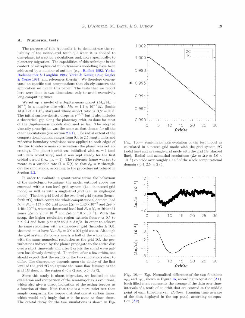
In order to evaluate in quantitative terms the behaviourof the nested-grid technique, the model outlined above wasexecuted with a two-level grid system (i.e., in nested-gridmode) as well as with a single-level grid (i.e., in single-gridmode). The first grid level of the two-level grid system (hence-forth 2G), which covers the whole computational domain, hadNr ×Nφ = 147×455 grid zones (∆r ≃ 1.46×10−2 and ∆φ ≃1.40×10−2), whereas the second level had Nr×Nφ = 264×464zones (∆r ≃ 7.3 × 10−3 and ∆φ ≃ 7.0 × 10−3). With thissetup, the higher resolution region extends from r ≃ 0.5 tor ≃ 2.4 and from φ ≃ π/2 to φ ≃ 3π/2. In order to achievethe same resolution with a single-level grid (henceforth 1G),the mesh must haveNr×Nφ = 290×904 grid zones. Althoughthe grid system 2G covers nearly a half of the whole domainwith the same numerical resolution as the grid 1G, the per-turbations induced by the planet propagate to the entire discover a short time-scale and after 5 orbits the spiral wave pat-tern has already developed. Therefore, after a few orbits, oneshould expect that the results of the two simulations start todiffer. The discrepancy depends upon the ability of the firstlevel of the grid 2G to capture the same flow features as thegrid 1G does, in the region φ < π/2 and φ > 3π/2.

Since this study is about migration, we focused on theevaluation and comparison of the semi-major axis evolutions,which also give a direct indication of the acting torques asa function of time. Note that this is a more strict test thansimply comparing the torque distributions at certain times,which would only imply that a is the same at those times.The orbital decay for the two simulations is shown in Fig-

Fig. 15.— Semi-major axis evolution of the test model ascalculated in a nested-grid mode with the grid system 2G(solid line) and in a single-grid mode with the grid 1G (dashedline). Radial and azimuthal resolutions (∆r ≃ ∆φ ≃ 7.0 ×10−3) coincide over roughly a half of the whole computationaldomain ([0.4, 2.5]× 2π).

Fig. 16.— Top. Normalised difference of the two functionsa2G and a1G, shown in Figure 15, according to equation (A1).Each filled circle represents the average of the data over time-intervals of a tenth of an orbit that are centred at the middlepoint of each time-interval. Bottom. Running time averageof the data displayed in the top panel, according to equa-tion (A2).


ure 15. The solid and dashed lines pertain to grids 2G and1G, respectively. To estimate the differences in more detail,we computed the normalised difference

∆a

a= 2

(

aII − aI

aII + aI

)

, (A1)

where the labels I and II identify the used grids 1G and 2G,respectively. Since the time-step is different in the two sim-ulations, a1G and a2G were averaged over time-intervals of0.1 orbits and the value measured from equation (A1) wasassigned to the central time of each interval. As shown inthe top panel of Figure 16, ∆a/a is typically a few times10−5 and it doesn’t increase beyond 1.5× 10−4. The bottompanel of Figure 16 illustrates the running time average of thenormalised difference

⟨

∆a

a

⟩

t

=1

t

∫ t

0

∆a

adt′, (A2)

which indicates that the discrepancies in the orbital evolu-tions are on average around a few times 10−3 per cent.

From the viewpoint of the computational load, the ad-vantage of the nested-grid technique is remarkable: in thecomputations reported above, the time-step required for nu-merical stability by grid 2G (first level) is twice as long asthat required by grid 1G and so the time needed to completeone orbital period is twice as short. It is also worthwhile topoint out that the refinement capabilities of the nested-gridstrategy does not reduce the accuracy of the numerical algo-rithm, which strictly remains second-order accurate in spacesince the mesh step size is always constant on each grid level.

For the sake of completeness, we show a test on the ac-celerated grid technique that we implemented and employedin this work. Other tests (not reported here) on the angu-lar momentum conservation of both the disc and the planetproved that conservation was achieved down to the machineprecision. Thus, we refer to a more relevant situation andshow how the migration calculated in a reference frame ro-tating with a variable Ω compares to that calculated in auniformly rotating grid with Ω = Ω0 =

√

GM∗/a30. The

outcome of such comparison is illustrated in Figure 17. Wecomputed the normalised difference (top panel) and the run-ning time average (bottom panel), where the quantity aII inequation (A1) was obtained from the grid 1G with Ω 6= 0while the quantity aI was obtained from the grid 1G withstatic rotation (i.e., Ω = 0). As Figure 17 proves, the dis-crepancy between the two semi-major axis evolutions is notsignificant. It has to be stressed that although the planetmoves on a “continuous” path, the gravitational potentialis centred in a grid zone. Therefore, results cannot be ex-actly the same since the planet’s trajectory through the gridcentres is different in the two simulations. In fact, in themodel with Ω 6= 0 there is only radial motion due to mi-gration, thus the time taken by the planet to cross a gridzone is ∆r/a ≃ (∆r/a) τM. Instead, in the other model, theazimuthal drift soon becomes the fastest component of theplanet’s motion and the time needed to cross a grid zone is

then given by ∆φ/ |ΩK − Ω0| or (∆φ/2π)

[

1−√

(a/a0)3

]−1

orbits. For instance, when ∆r/a ≈ ∆φ and a = 0.99 a0, in

Fig. 17.— Comparison between the orbital evolutions com-puted with the grid 1G setting a constant rotation rateΩ = Ω0 =

√

GM∗/a30 and a variable rate (i.e., Ω 6= 0) such

that the planet’s azimuthal position remains constant. Top.Normalised difference (see eq. [A1]) sampled as in the toppanel of Figure 16. Bottom. Running time average of thedata displayed in the top panel.

a steadily rotating grid a planet undergoes ≈ τM/11 ≈ 300(see Fig. 15) as many encounters with the grid centres as itdoes in a grid rotating at a variable rate where there is noazimuthal drift.

gennaro d’angelo and matthew r. bate - arxiv · gennaro d’angelo and matthew r. bate ... in the...

Documents