genetic interaction network - hcbravo
TRANSCRIPT
Yeast highthrouput doubleknockdown assay~5000 genes~800k interactions
http://www.geneticinteractions.org/
Costanzo et al. (2016) Science. DOI: 10.1126/science.aaf1420
Genetic Interaction Network
1 / 60
Yeast highthrouput doubleknockdown assay~5000 genes~800k interactions
http://www.geneticinteractions.org/
Costanzo et al. (2016) Science. DOI: 10.1126/science.aaf1420
Genetic Interaction Network
2 / 60
Genetic Interaction NetworkNumber of vertices: 2803Number of edges: 67,268
3 / 60
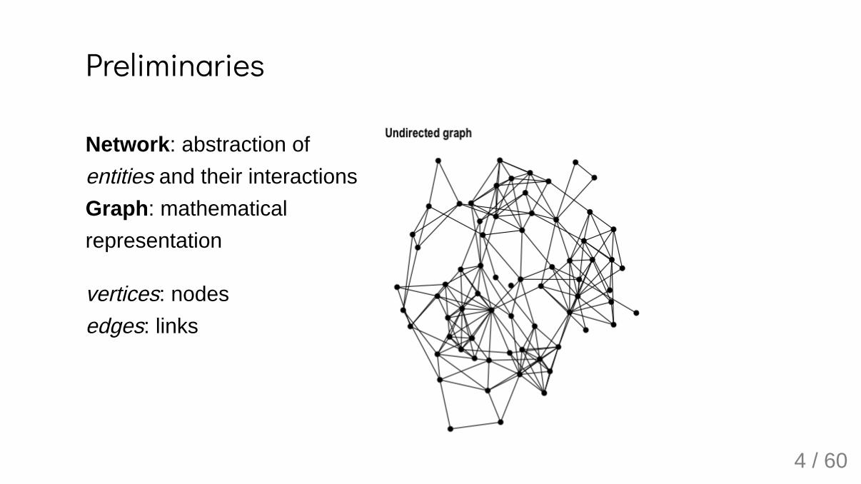
Network: abstraction ofentities and their interactions Graph: mathematicalrepresentation
vertices: nodes edges: links
Preliminaries
4 / 60
Network: abstraction ofentities and their interactions Graph: mathematicalrepresentation
vertices: nodes edges: links
Preliminaries
5 / 60
Network statistics: notationNumber of vertices:
In our example: number of genes
n
6 / 60
Network statistics: notationNumber of vertices:
In our example: number of genes
Number of edges:
In our example: number of genetic interactions
n
m
7 / 60
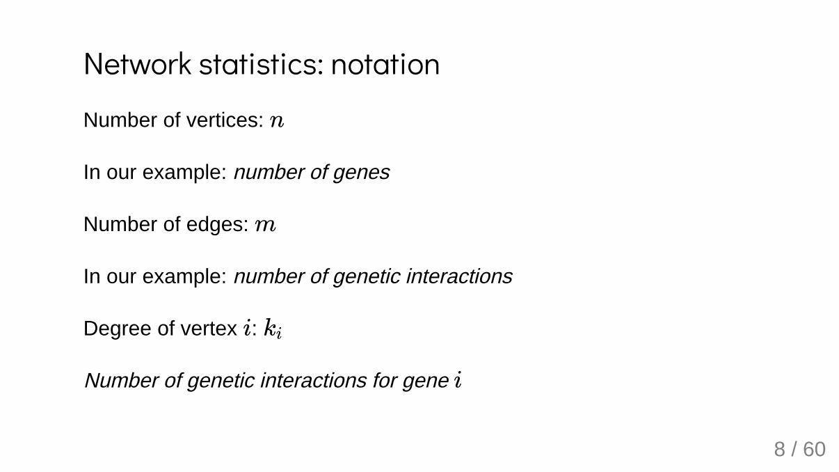
Network statistics: notationNumber of vertices:
In our example: number of genes
Number of edges:
In our example: number of genetic interactions
Degree of vertex :
Number of genetic interactions for gene
n
m
i ki
i
8 / 60
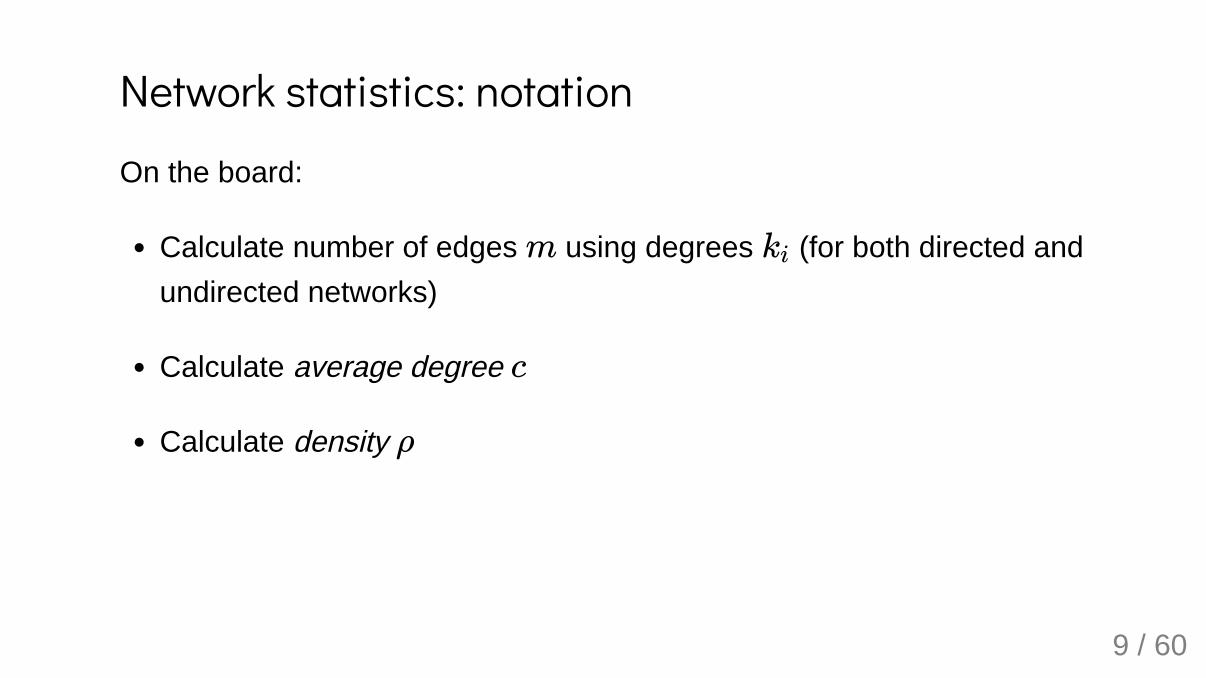
Network statistics: notationOn the board:
Calculate number of edges using degrees (for both directed andundirected networks)
Calculate average degree
Calculate density
m ki
c
ρ
9 / 60
Network statistics: notationOn the board:
Calculate number of edges using degrees (for both directed andundirected networks)
Calculate average degree
Calculate density
In our example:
Average degree: 47.9971459 Density: 0.0171296
m ki
c
ρ
10 / 60
(On the board)Number of edges using degrees (undirected)
Number of edges using degrees (directed)
m =n
∑i=1
ki1
2
m =n
∑i=1
kini =
n
∑i=1
kouti
11 / 60
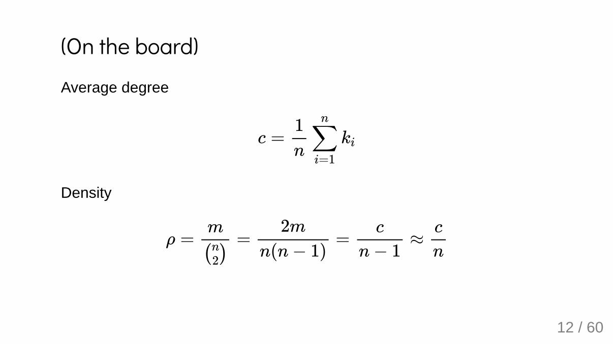
(On the board)Average degree
Density
c =n
∑i=1
ki1
n
ρ = = = ≈m
( )n2
2m
n(n − 1)
c
n − 1
c
n
12 / 60
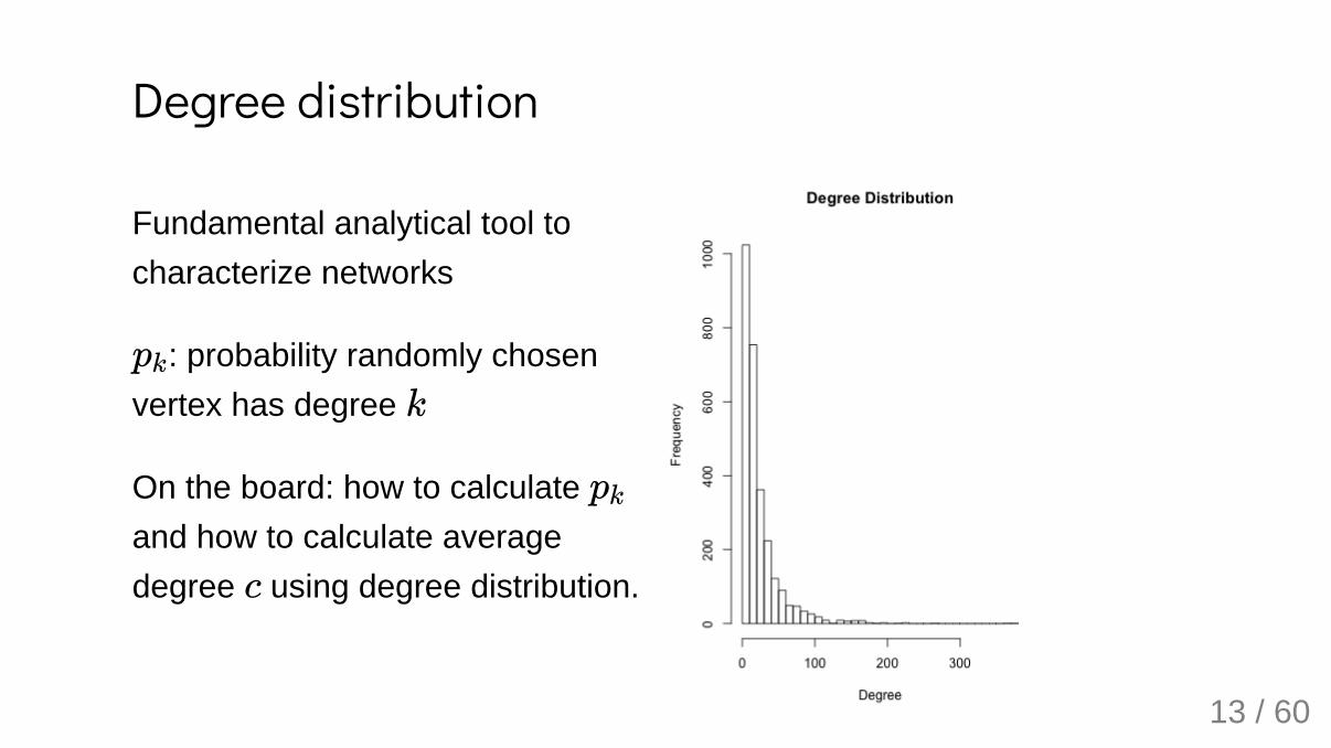
Fundamental analytical tool tocharacterize networks
: probability randomly chosenvertex has degree
On the board: how to calculate and how to calculate averagedegree using degree distribution.
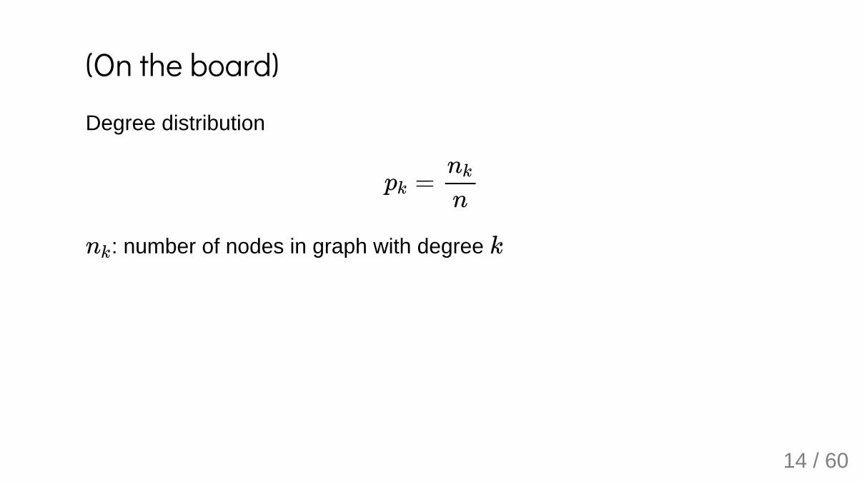
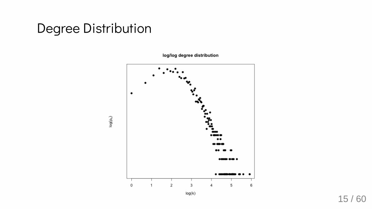
Degree distribution
pkk
pk
c
13 / 60
(On the board)Degree distribution
: number of nodes in graph with degree
pk =nk
n
nk k
14 / 60
Degree Distribution
15 / 60
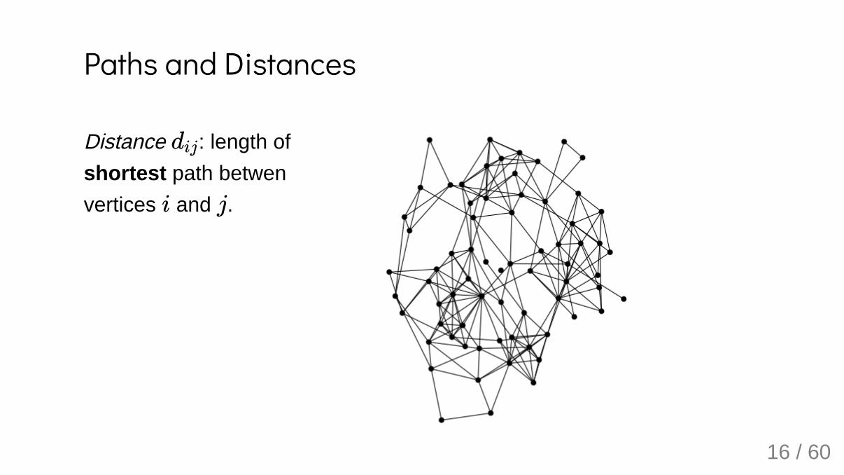
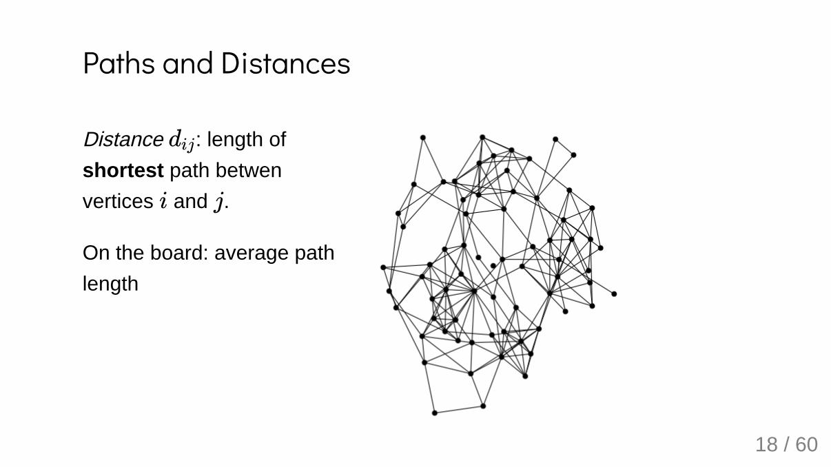
Distance : length ofshortest path betwenvertices and .
Paths and Distances
dij
i j
16 / 60
Distance : length ofshortest path betwenvertices and .
Diameter: longest shortestpath
Paths and Distances
dij
i j
maxij dij
17 / 60
Distance : length ofshortest path betwenvertices and .
On the board: average pathlength
Paths and Distances
dij
i j
18 / 60
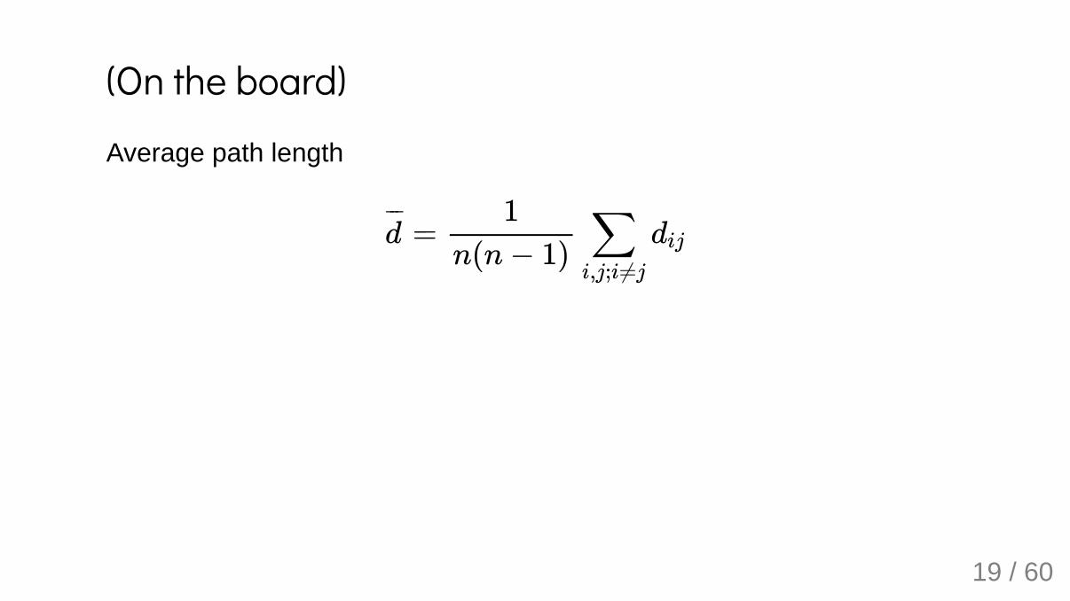
(On the board)Average path length
¯̄̄d = ∑
i,j;i≠j
dij1
n(n − 1)
19 / 60
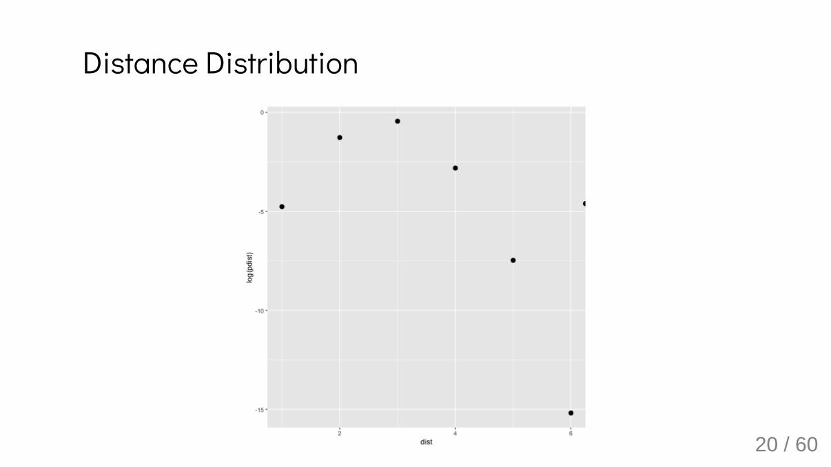
Distance Distribution
20 / 60
Distances and pathsBy convention: if there is no path between vertices and then i j dij = ∞
21 / 60
Distances and pathsBy convention: if there is no path between vertices and then
Vertices and are connected if
i j dij = ∞
i j dij < ∞
22 / 60
Distances and pathsBy convention: if there is no path between vertices and then
Vertices and are connected if
Graph is connected if for all ,
i j dij = ∞
i j dij < ∞
dij < ∞ i j
23 / 60
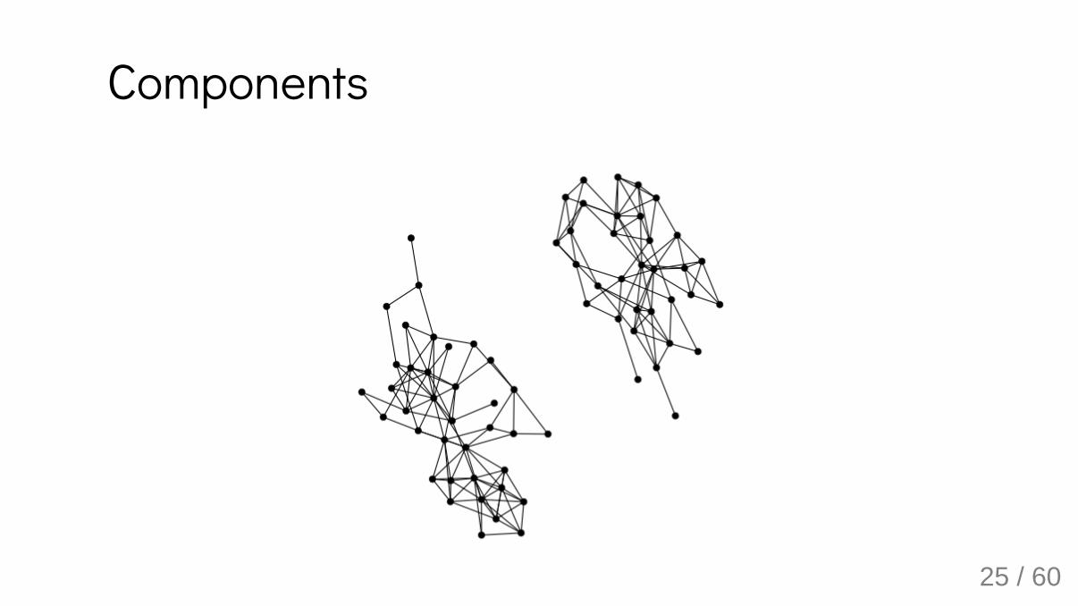
Distances and pathsBy convention: if there is no path between vertices and then
Vertices and are connected if
Graph is connected if for all ,
Components maximal subset of connected components
i j dij = ∞
i j dij < ∞
dij < ∞ i j
24 / 60
Components
25 / 60
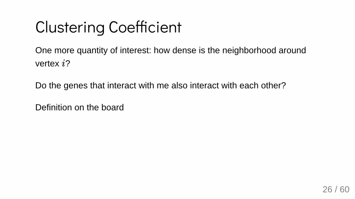
Clustering Coe�cientOne more quantity of interest: how dense is the neighborhood aroundvertex ?
Do the genes that interact with me also interact with each other?
Definition on the board
i
26 / 60
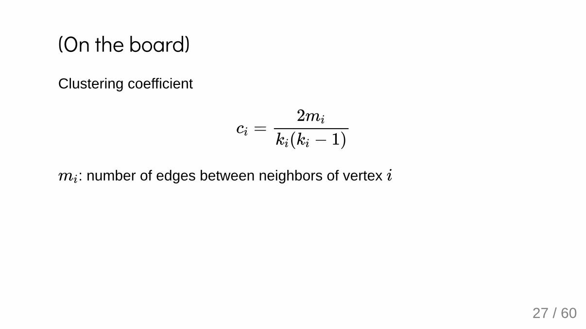
(On the board)Clustering coefficient
: number of edges between neighbors of vertex
ci =2mi
ki(ki − 1)
mi i
27 / 60
Clustering coe�cient
28 / 60
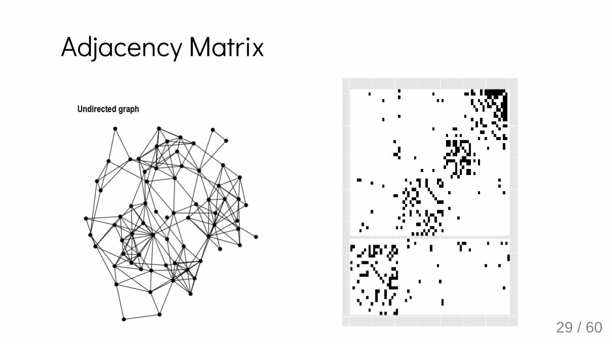
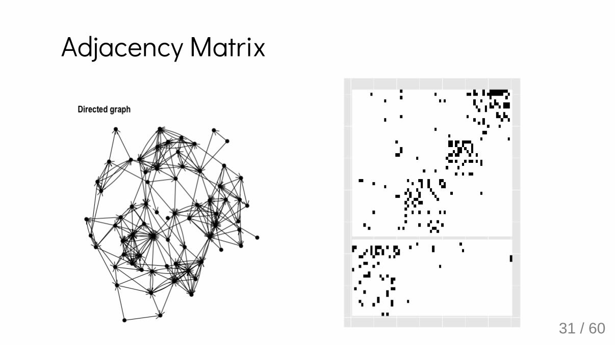
Adjacency Matrix
29 / 60
On the board:
DefinitionComputing degree with adj.matrixComputing num. edges withadj. matrixComputing paths with adj. matrix
Adjacency Matrix
m
30 / 60
Adjacency Matrix
31 / 60
Weighted networksEdges are assigned a weight indicating quantitative property ofinteraction
32 / 60
Weighted networksEdges are assigned a weight indicating quantitative property ofinteraction
Strength of genetic interaction (evidence from experiment)
Rates in a metabolic network
Spatial distance in an ecological network
33 / 60
Adjacency matrix contains weights instead of 0/1 entries
34 / 60
Adjacency matrix contains weights instead of 0/1 entries
Path lengths are the sum of edge weights in a path
35 / 60
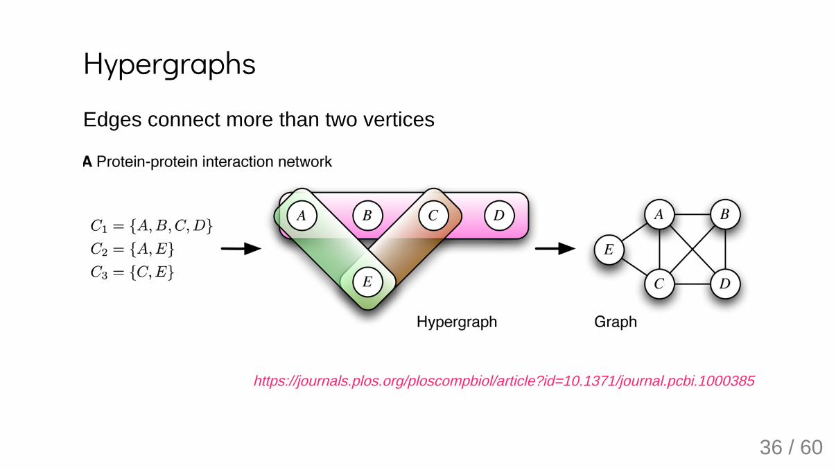
https://journals.plos.org/ploscompbiol/article?id=10.1371/journal.pcbi.1000385
HypergraphsEdges connect more than two vertices
36 / 60
Acyclic graphs
Single path between any pair ofvertices
https://www.sciencedirect.com/science/article/pii/S0981942817304321
Trees
37 / 60
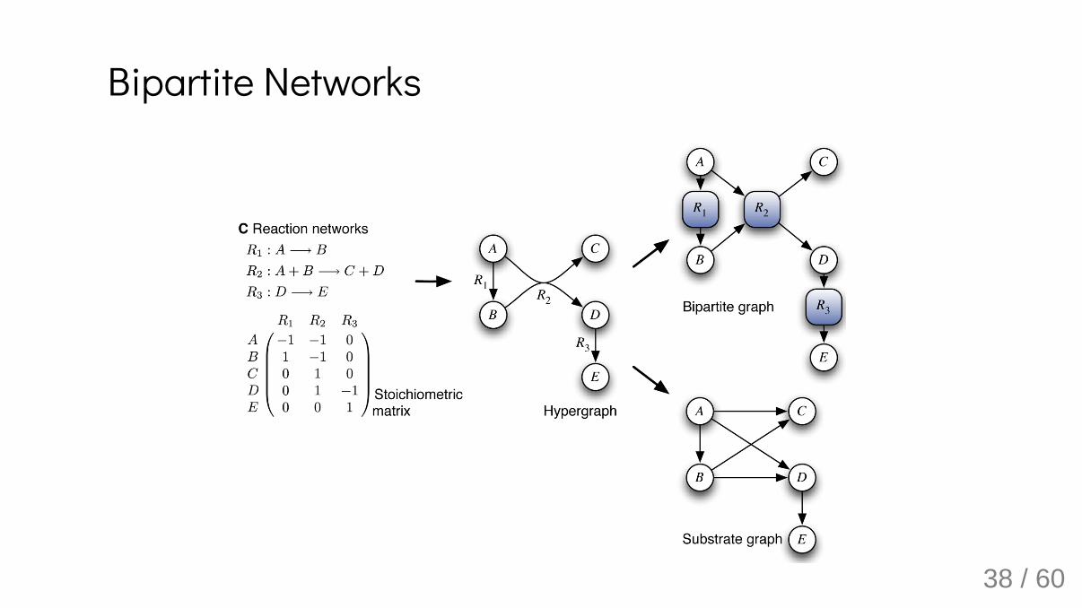
Bipartite Networks
38 / 60
Bipartite NetworksWe use an Incidence Matrix instead of Adjacency Matrix
(On the board): definition
B
39 / 60
Bipartite Networks
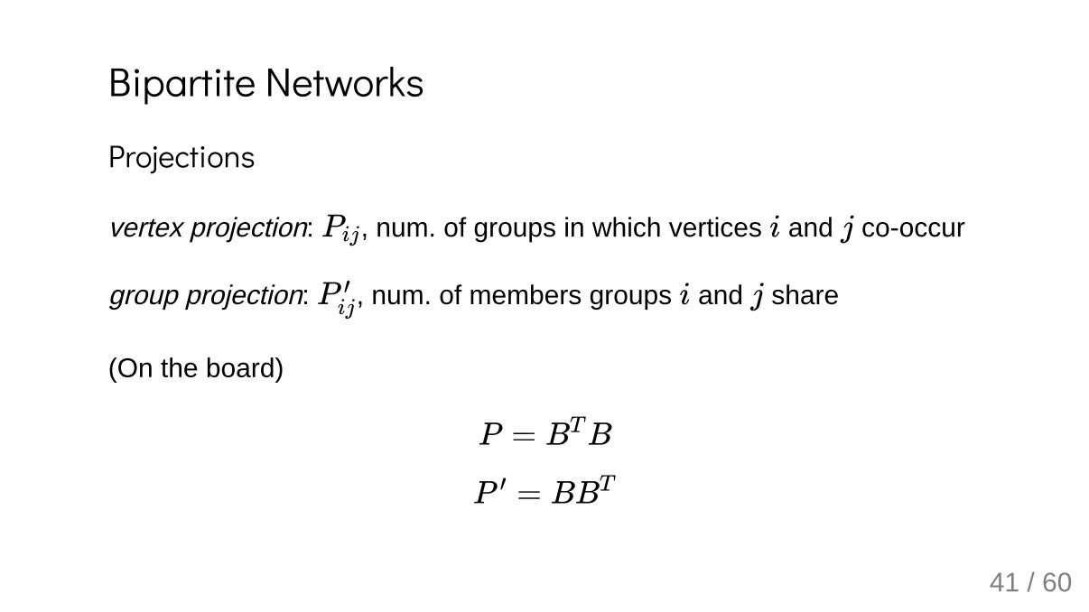
Projections
vertex projection: , num. of groups in which vertices and cooccur
group projection: , num. of members groups and share
Pij i j
P ′ij i j
40 / 60
Bipartite Networks
Projections
vertex projection: , num. of groups in which vertices and cooccur
group projection: , num. of members groups and share
(On the board)
Pij i j
P ′ij i j
P = BTB
P ′ = BBT
41 / 60
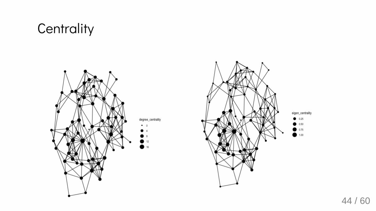
What are the importantnodes in the network?
What are central nodes inthe network?
Centrality
42 / 60
Centrality
Undirected Graphs
Eigenvalue Centrality
Directed Graphs
Katz CentralityPagerank
43 / 60
Centrality
44 / 60
What are the importantedges in the network?
What are edges that mayconnect clusters of nodes inthe network?
Betweenness
45 / 60
GirvanNewman Algorithm hierarchical method topartition nodes intocommunities using edgebetweenness
Betweenness
46 / 60
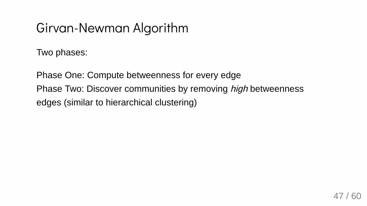
Girvan-Newman AlgorithmTwo phases:
Phase One: Compute betweenness for every edge Phase Two: Discover communities by removing high betweennessedges (similar to hierarchical clustering)
47 / 60
Girvan-Newman Algorithm
Calculating Betweenness
Formally, : fraction of vertex pairs whereshortest path crossess edge
Path Counting: For each vertex , use breadthfirstsearch to countnumber of shortest paths through each edge in graph between andevery other vertex .
Sum result across vertices for each edge , and divide by two
Presentation from Mining Massive Datasets Leskovec, et al.http://mmds.org/ (Ch. 10)
betweenness(e) (x, y)
e
x
e x
y
e
48 / 60
Girvan-Newman Algorithm
Counting Paths
Algorithm (starting from node )
1. Construct breadthfirst search tree2. (Root>Leaf) Label each vertex with the number of shortest pathsbetween and : sum of labels of parents
3. (Leaf>Root) Count the (weighted) number of shortest paths that gothrough each edge: next slide
x
v
x v
49 / 60
Girvan-Newman Algorithm
Counting Paths
Step 3, counting number of shortest paths through each edge
a. Leafs in search tree get a credit of
b. Incoming edge to vertex in search tree gets credit
: number of shortest paths between and (computed in Step 2)sum is over parents of
v Cv = 1
ei = (yi, v) v
Cei = Cv ∗pi
∑j pj
pi x yi∑j v
50 / 60
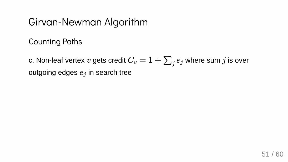
Girvan-Newman Algorithm
Counting Paths
c. Nonleaf vertex gets credit where sum is over
outgoing edges in search tree
v Cv = 1 + ∑j ej j
ej
51 / 60
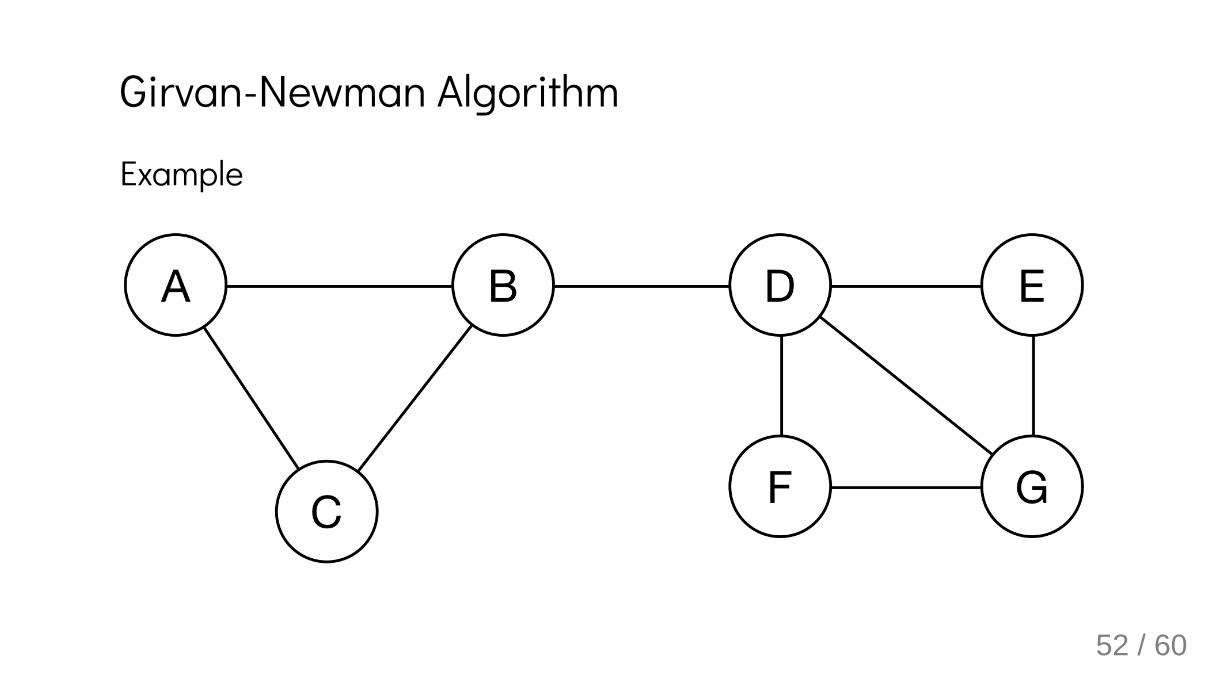
Girvan-Newman Algorithm
Example
52 / 60
Resources
Cross-language
igraph: http://igraph.org/ Boost Graph Library:https://www.boost.org/doc/libs/1_71_0/libs/graph/doc/
53 / 60
Resources
Python
igraphnetworkx
54 / 60
Resources
R
Workhorses:
igraphRgraphviz
Tidyverse (https://tidyverse.org):
tidygraphggraph
55 / 60
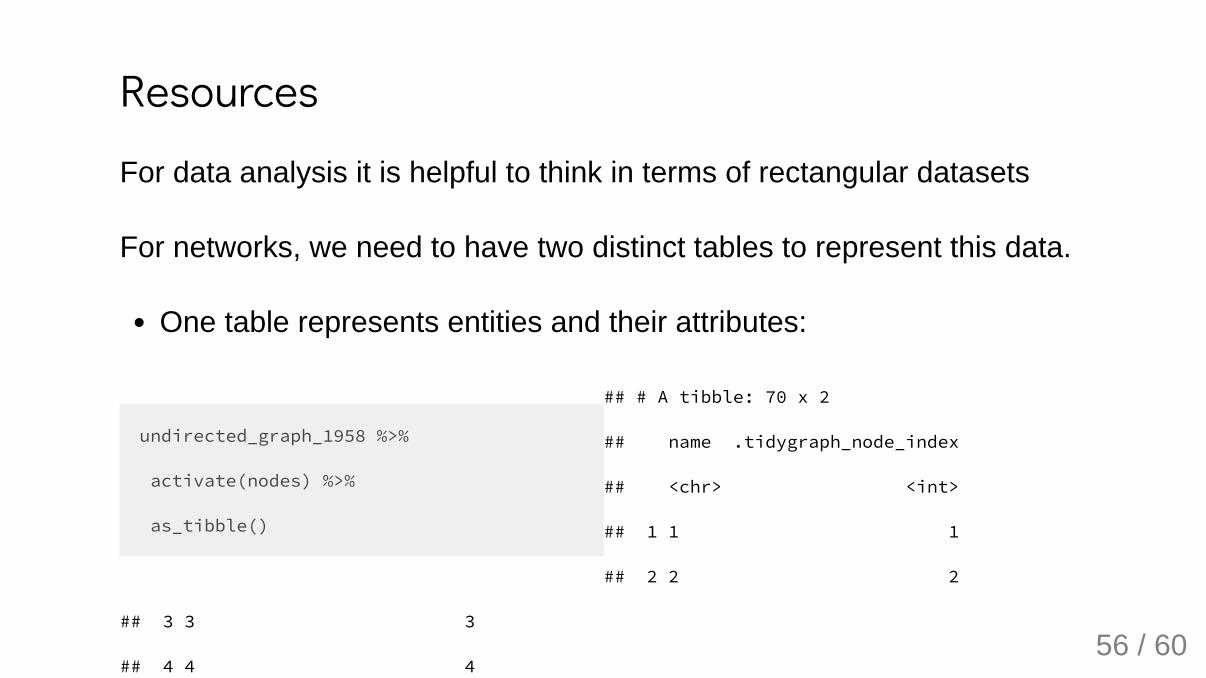
undirected_graph_1958 %>%
activate(nodes) %>%
as_tibble()
ResourcesFor data analysis it is helpful to think in terms of rectangular datasets
For networks, we need to have two distinct tables to represent this data.
One table represents entities and their attributes:
## # A tibble: 70 x 2
## name .tidygraph_node_index
## <chr> <int>
## 1 1 1
## 2 2 2
## 3 3 3
## 4 4 456 / 60
undirected_graph_1958 %>%
activate(edges) %>%
as_tibble()
ResourcesSecond table to represent edges and their attributes:
## # A tibble: 202 x 4
## from to .tidygraph_edge_index .orig_data
## <int> <int> <list> <list>
## 1 1 14 <int [2]> <tibble [2 × 3]>
## 2 1 16 <int [1]> <tibble [1 × 3]>
## 3 1 20 <int [1]> <tibble [1 × 3]>
## 4 1 21 <int [1]> <tibble [1 × 3]>
## 5 2 9 <int [1]> <tibble [1 × 3]>
## 6 2 21 <int [1]> <tibble [1 × 3]>
## 7 4 5 <int [2]> <tibble [2 × 3]> 57 / 60
Network-derived attributesBesides attributes measured for each node, we have seen we can derivenode and edge attributes based on the structure of the network.
For instance, we can compute the degree of a node, that is, the numberof edges incident to the node.
58 / 60
Network-derived attributes## # A tibble: 70 x 3
## name .tidygraph_node_index degree
## <chr> <int> <dbl>
## 1 1 1 4
## 2 2 2 2
## 3 3 3 0
## 4 4 4 5
## 5 5 5 5
## 6 6 6 5
## 7 7 7 3
## 8 8 8 5
## 9 9 9 6
undirected_graph_1958 <- undirected_graph_19
activate(nodes) %>%
mutate(degree = centrality_degree())
undirected_graph_1958 %>%
activate(nodes) %>%
as_tibble
59 / 60
Network-derived attributesThe distribution of newly created attributes are fundamental analyticaltools to characterize networks.
undirected_graph_1958 %>%
activate(nodes) %>%
as_tibble() %>%
group_by(degree) %>%
summarize(n=n()) %>%
ungroup() %>%
mutate(num_nodes = sum(n)) %>%
mutate(deg_prop = n / num_nodes) %>% 60 / 60
Network PreliminariesHéctor Corrada Bravo
University of Maryland, College Park, USA CMSC828O 20190904

Yeast highthrouput doubleknockdown assay~5000 genes~800k interactions
http://www.geneticinteractions.org/
Costanzo et al. (2016) Science. DOI: 10.1126/science.aaf1420
Genetic Interaction Network
1 / 60

Yeast highthrouput doubleknockdown assay~5000 genes~800k interactions
http://www.geneticinteractions.org/
Costanzo et al. (2016) Science. DOI: 10.1126/science.aaf1420
Genetic Interaction Network
2 / 60

Genetic Interaction NetworkNumber of vertices: 2803Number of edges: 67,268
3 / 60
Network: abstraction ofentities and their interactions Graph: mathematicalrepresentation
vertices: nodes edges: links
Preliminaries
4 / 60

Network: abstraction ofentities and their interactions Graph: mathematicalrepresentation
vertices: nodes edges: links
Preliminaries
5 / 60
Network statistics: notationNumber of vertices:
In our example: number of genes
n
6 / 60
Network statistics: notationNumber of vertices:
In our example: number of genes
Number of edges:
In our example: number of genetic interactions
n
m
7 / 60
Network statistics: notationNumber of vertices:
In our example: number of genes
Number of edges:
In our example: number of genetic interactions
Degree of vertex :
Number of genetic interactions for gene
n
m
i ki
i
8 / 60
Network statistics: notationOn the board:
Calculate number of edges using degrees (for both directed andundirected networks)
Calculate average degree
Calculate density
m ki
c
ρ
9 / 60

Network statistics: notationOn the board:
Calculate number of edges using degrees (for both directed andundirected networks)
Calculate average degree
Calculate density
In our example:
Average degree: 47.9971459 Density: 0.0171296
m ki
c
ρ
10 / 60

(On the board)Number of edges using degrees (undirected)
Number of edges using degrees (directed)
m =
n
∑i=1
ki
1
2
m =
n
∑i=1
kin
i=
n
∑i=1
kout
i
11 / 60
(On the board)Average degree
Density
c =n
∑i=1
ki
1
n
ρ = = = ≈m
( )n2
2m
n(n − 1)
c
n − 1
c
n
12 / 60
Fundamental analytical tool tocharacterize networks
: probability randomly chosenvertex has degree
On the board: how to calculate and how to calculate averagedegree using degree distribution.
Degree distribution
pk
k
pk
c
13 / 60
(On the board)Degree distribution
: number of nodes in graph with degree
pk =
nk
n
nk k
14 / 60
Degree Distribution
15 / 60
Distance : length ofshortest path betwenvertices and .
Paths and Distances
dij
i j
16 / 60

Distance : length ofshortest path betwenvertices and .
Diameter: longest shortestpath
Paths and Distances
dij
i j
maxij dij
17 / 60
Distance : length ofshortest path betwenvertices and .
On the board: average pathlength
Paths and Distances
dij
i j
18 / 60
(On the board)Average path length
¯̄̄d = ∑
i,j;i≠j
dij1
n(n − 1)
19 / 60
Distance Distribution
20 / 60
Distances and pathsBy convention: if there is no path between vertices and then i j dij = ∞
21 / 60

Distances and pathsBy convention: if there is no path between vertices and then
Vertices and are connected if
i j dij = ∞
i j dij < ∞
22 / 60

Distances and pathsBy convention: if there is no path between vertices and then
Vertices and are connected if
Graph is connected if for all ,
i j dij = ∞
i j dij < ∞
dij < ∞ i j
23 / 60
Distances and pathsBy convention: if there is no path between vertices and then
Vertices and are connected if
Graph is connected if for all ,
Components maximal subset of connected components
i j dij = ∞
i j dij < ∞
dij < ∞ i j
24 / 60
Components
25 / 60
Clustering Coe�cientOne more quantity of interest: how dense is the neighborhood aroundvertex ?
Do the genes that interact with me also interact with each other?
Definition on the board
i
26 / 60
(On the board)Clustering coefficient
: number of edges between neighbors of vertex
ci =2mi
ki(ki − 1)
mi i
27 / 60

Clustering coe�cient
28 / 60
Adjacency Matrix
29 / 60

On the board:
DefinitionComputing degree with adj.matrixComputing num. edges withadj. matrixComputing paths with adj. matrix
Adjacency Matrix
m
30 / 60
Adjacency Matrix
31 / 60
Weighted networksEdges are assigned a weight indicating quantitative property ofinteraction
32 / 60
Weighted networksEdges are assigned a weight indicating quantitative property ofinteraction
Strength of genetic interaction (evidence from experiment)
Rates in a metabolic network
Spatial distance in an ecological network
33 / 60
Adjacency matrix contains weights instead of 0/1 entries
34 / 60

Adjacency matrix contains weights instead of 0/1 entries
Path lengths are the sum of edge weights in a path
35 / 60
https://journals.plos.org/ploscompbiol/article?id=10.1371/journal.pcbi.1000385
HypergraphsEdges connect more than two vertices
36 / 60

Acyclic graphs
Single path between any pair ofvertices
https://www.sciencedirect.com/science/article/pii/S0981942817304321
Trees
37 / 60
Bipartite Networks
38 / 60
Bipartite NetworksWe use an Incidence Matrix instead of Adjacency Matrix
(On the board): definition
B
39 / 60

Bipartite Networks
Projections
vertex projection: , num. of groups in which vertices and cooccur
group projection: , num. of members groups and share
Pij i j
P ′
ij i j
40 / 60
Bipartite Networks
Projections
vertex projection: , num. of groups in which vertices and cooccur
group projection: , num. of members groups and share
(On the board)
Pij i j
P ′
ij i j
P = BT B
P ′= BBT
41 / 60

What are the importantnodes in the network?
What are central nodes inthe network?
Centrality
42 / 60

Centrality
Undirected Graphs
Eigenvalue Centrality
Directed Graphs
Katz CentralityPagerank
43 / 60
Centrality
44 / 60

What are the importantedges in the network?
What are edges that mayconnect clusters of nodes inthe network?
Betweenness
45 / 60

GirvanNewman Algorithm hierarchical method topartition nodes intocommunities using edgebetweenness
Betweenness
46 / 60
Girvan-Newman AlgorithmTwo phases:
Phase One: Compute betweenness for every edge Phase Two: Discover communities by removing high betweennessedges (similar to hierarchical clustering)
47 / 60
Girvan-Newman Algorithm
Calculating Betweenness
Formally, : fraction of vertex pairs whereshortest path crossess edge
Path Counting: For each vertex , use breadthfirstsearch to countnumber of shortest paths through each edge in graph between andevery other vertex .
Sum result across vertices for each edge , and divide by two
Presentation from Mining Massive Datasets Leskovec, et al.http://mmds.org/ (Ch. 10)
betweenness(e) (x, y)
e
x
e x
y
e
48 / 60

Girvan-Newman Algorithm
Counting Paths
Algorithm (starting from node )
1. Construct breadthfirst search tree2. (Root>Leaf) Label each vertex with the number of shortest pathsbetween and : sum of labels of parents
3. (Leaf>Root) Count the (weighted) number of shortest paths that gothrough each edge: next slide
x
v
x v
49 / 60
Girvan-Newman Algorithm
Counting Paths
Step 3, counting number of shortest paths through each edge
a. Leafs in search tree get a credit of
b. Incoming edge to vertex in search tree gets credit
: number of shortest paths between and (computed in Step 2)sum is over parents of
v Cv = 1
ei = (yi, v) v
Cei= Cv ∗
pi
∑j pj
pi x yi
∑j v
50 / 60
Girvan-Newman Algorithm
Counting Paths
c. Nonleaf vertex gets credit where sum is over
outgoing edges in search tree
v Cv = 1 +∑j ej j
ej
51 / 60
Girvan-Newman Algorithm
Example
52 / 60

Resources
Cross-language
igraph: http://igraph.org/ Boost Graph Library:https://www.boost.org/doc/libs/1_71_0/libs/graph/doc/
53 / 60

Resources
Python
igraphnetworkx
54 / 60

Resources
R
Workhorses:
igraphRgraphviz
Tidyverse (https://tidyverse.org):
tidygraphggraph
55 / 60
undirected_graph_1958 %>%
activate(nodes) %>%
as_tibble()
ResourcesFor data analysis it is helpful to think in terms of rectangular datasets
For networks, we need to have two distinct tables to represent this data.
One table represents entities and their attributes:
## # A tibble: 70 x 2
## name .tidygraph_node_index
## <chr> <int>
## 1 1 1
## 2 2 2
## 3 3 3
## 4 4 456 / 60

undirected_graph_1958 %>%
activate(edges) %>%
as_tibble()
ResourcesSecond table to represent edges and their attributes:
## # A tibble: 202 x 4
## from to .tidygraph_edge_index .orig_data
## <int> <int> <list> <list>
## 1 1 14 <int [2]> <tibble [2 × 3]>
## 2 1 16 <int [1]> <tibble [1 × 3]>
## 3 1 20 <int [1]> <tibble [1 × 3]>
## 4 1 21 <int [1]> <tibble [1 × 3]>
## 5 2 9 <int [1]> <tibble [1 × 3]>
## 6 2 21 <int [1]> <tibble [1 × 3]>
## 7 4 5 <int [2]> <tibble [2 × 3]> 57 / 60

Network-derived attributesBesides attributes measured for each node, we have seen we can derivenode and edge attributes based on the structure of the network.
For instance, we can compute the degree of a node, that is, the numberof edges incident to the node.
58 / 60
Network-derived attributes## # A tibble: 70 x 3
## name .tidygraph_node_index degree
## <chr> <int> <dbl>
## 1 1 1 4
## 2 2 2 2
## 3 3 3 0
## 4 4 4 5
## 5 5 5 5
## 6 6 6 5
## 7 7 7 3
## 8 8 8 5
## 9 9 9 6
undirected_graph_1958 <- undirected_graph_19
activate(nodes) %>%
mutate(degree = centrality_degree())
undirected_graph_1958 %>%
activate(nodes) %>%
as_tibble
59 / 60

Network-derived attributesThe distribution of newly created attributes are fundamental analyticaltools to characterize networks.
undirected_graph_1958 %>%
activate(nodes) %>%
as_tibble() %>%
group_by(degree) %>%
summarize(n=n()) %>%
ungroup() %>%
mutate(num_nodes = sum(n)) %>%
mutate(deg_prop = n / num_nodes) %>% 60 / 60