genetic diversity of native and crossbreed sheep breeds in
TRANSCRIPT

GENETIC DIVERSITY OF NATIVE AND CROSSBREED SHEEP BREEDS IN ANATOLIA
A THESIS SUBMITTED TO THE GRADUATE SCHOOL OF NATURAL AND APPLIED SCIENCES
OF MIDDLE EAST TECHNICAL UNIVERSITY
BY
EVREN KOBAN
IN PARTIAL FULFILLMENT OF THE REQUIREMENTS FOR
THE DEGREE OF DOCTOR OF PHILOSOPHY IN
DEPARTMENT OF BIOLOGY
DECEMBER 2004

Approval of the Graduate School of Natural and Applied Sciences
________________________
Prof. Dr. Canan ÖZGEN
Director
I certify that this thesis satisfies all the requirements as a thesis for the degree of
Doctor of Philosophy.
________________________
Prof. Dr. Semra KOCABIYIK
Head of the Department
This is to certify that we have read this thesis and that in our opinion it is fully
adequate, in scope and quality, as a thesis for the degree of Doctor of Philosophy.
________________________
Prof. Dr. �nci TOGAN
Supervisor
Examining Committee Members
Prof. Dr. Zeki KAYA (METU, BIO) _________________
Prof. Dr. �nci TOGAN (METU, BIO) _________________
Prof. Dr. M. �hsan SOYSAL (Trakya Ünv., TZF) _________________
Prof. Dr. Mehmet N�ZAMLIO�LU (Selçuk Ünv., Vet. Fak.) _________________
Prof. Dr. Okan ERTU�RUL (Ankara Ünv., Vet. Fak.) _________________

iii
I hereby declare that all information in this document has been obtained and
presented in accordance with academic rules and ethical conduct. I also declare that,
as required by these rules and conduct, I have fully cited and referenced all material
and results that are not original to this work.
Evren KOBAN

iv
ABSTRACT
GENETIC DIVERSITY OF NATIVE AND CROSSBREED SHEEP BREEDS IN
ANATOLIA
Koban, Evren
Ph.D., Department of Biology
Supervisor: Prof. Dr. �nci Togan
December 2004, 125 pages
In this study the genetic diversity in Turkish native sheep breeds was
investigated based on microsatellite DNA loci. In total, 423 samples from 11 native
and crossbreed Turkish sheep breeds (Akkaraman, Morkaraman, Kıvırcık, �vesi,
Da�lıç, Karayaka, Hem�in, Norduz, Kangal, Konya Merinosu, Türkgeldi) and one
Iraqi breed (Hamdani) were analyzed by sampling from breeding farms and local
breeders.
After excluding close relatives by Kinship analysis, the genetic variation
within breeds was estimated as gene diversities (HE), which ranged between 0.686
and 0.793. The mean number of observed alleles (MNA) ranged between 5.8 and
11.8. The allele frequency distribution across Turkey showed no gradient from east
to west expected in accordance with the Neolithic Demic Diffusion model. The
differentiation between different samples of Akkaraman, Da�lıç and Karayaka
breeds was tested by FST index. Akkaraman1 sample from the breeding farm was

v
significantly (P<0.001) different from the other two Akkaraman samples. Deviation
from HW expectations observed for Akkaraman1, �vesi, Morkaraman and Hem�in
breeds. AMOVA analysis revealed that most of the total genetic variation (~90%)
was partitioned within the individuals. In parallel to this observation, when factorial
correspondence analysis and shared alleles distances were used to analyze the
relationship between the individuals of the breeds, there was no clear discrimination
between breeds. Moreover, NJ tree constructed based on DA genetic distance, and PC
analyses were used to analyze among breed differentiation. Delaunay Network drew
4 genetic boundaries (two of them being parallel to geographic boundaries) between
breeds. All the results indicated that Kıvırcık was the most differentiated breed.
Finally, Mantel Test and Bottleneck analysis did not reveal a significant result.
Kıvırcık breed, among all native Turkish breeds, was found to be the
genetically closest to the European breeds based on the loci analyzed. The genetic
variation in Turkish breeds was not much higher than that of European breeds, which
might be a consequence of the recent sharp decrease in sheep number.
Keywords: Genetic variation, microsatellite, sheep, Turkish breeds.

vi
ÖZ
ANADOLU YERL� VE MELEZ KOYUN IRKLARININ GENET�K ÇE��TL�L���
Koban, Evren
Doktora, Biyoloji Bölümü
Tez Yöneticisi: Prof. Dr. �nci Togan
Aralık 2004, 125 sayfa
Bu çalı�mada, Türk koyun ırklarında mevcut genetic çe�itlilik Mikrosatelit
DNA lokusları kullanılarak incelenmi�tir. Devlet üretim çiftlikleri, üniversite üretim
çiftlikleri ve yerel yeti�tiricilerin elinde bulunan sürülerden yerli ve melez onbir Türk
ırkı (Akkaraman, Morkaraman, Kıvırcık, �vesi, Da�lıç, Karayaka, Hem�in, Narduz,
Kangal, Konya Merinosu, Türkgeldi) ile bireyleri Irak'tan getirilmi� yabancı bir ırkı
(Hamdani) temsil eden toplam 423 örnek bu çalı�mada kullanılmı�tır.
Öncelikle üretim çiftliklerinden toplanan populasyonlardan akrabalık derecesi
yüksek bireylere ait veriler yakınlık (kinship) analizinin sonuçları do�rultusunda
çıkartılmı�tır. Genetik varyasyonun ölçütlerinden beklenen heterozigotluk (HE) 0.686
ile 0.793 arasında, ortalama gözlenen alel sayıları (OAS) ise 5.8 ile 11.8 arasında
de�i�mi�tir. Türkiye üzerinde alel frekans da�ılımları Neolitik Gruplarca Yayılma
Modeli'nin bekledi�i gibi bir de�i�im göstermemi�tir. FST indeksi Akkaraman,
Karayaka ve Da�lıç'ta aynı ırkın farklı populasyonlarındaki farklıla�mayı ölçmek
için kullanılmı�tır ve yeti�tirme çiftli�inden alınan Akkarman1'in di�er iki
vii
Akkaraman populasyonundan istatistiki önemle (P<0.001) farklı oldu�u
bulunmu�tur. FIS indeksi ile ırklar Hardy-Weinberg dengesi açısından test edilmi�,
Akkaraman1, �vesi, Morkaraman ve Hem�in'de H-W'den sapma tespit edilmi�tir.
AMOVA analizi toplam genetik varyasyonun büyük bir kısmının (~%90) bireyler
içinde ayrı�arak payla�ıldı�ını göstermi�tir. Paralel sonuçlar bireyler arası genetik
ili�kinin incelendi�i faktöryel benzerlik analizi ve alel payla�ım uzaklı�ı ile de elde
edilmi� ve ırklar arası belirgin bir fark görülmemi�tir. DA genetik uzaklı�ı ile çizilen
NJ a�acı ve temel ögeler analizi ise populasyonlar arası farklıla�mayı incelemek için
kullanılmı�tır. Delaunay örgüsü ırklar arasında 4 adet (ikisi co�rafi bariyer ile
paralel) genetik sınır belirlemi�tir. Sonuçların hepsi Kıvırcık'ın di�erlerinden çok
farklı oldu�u yönündedir. Mantel testi ve Bottleneck testi istatistiksel olarak anlamlı
bir sonuç ortaya koymamı�tır.
Avrupa ırklarının ço�una genetik olarak en yakın bulunan Kıvırcık'tır. Türk
ırklarında Avrupa ırklarından farklı ve yüksek bir genetik çe�itlilik belirlenmemi�tir.
Bunda son yıllarda koyun sayısında ya�anan hızlı dü�ü� etkili olmu� olabilir.
Anahtar Kelimeler: Genetik varyasyon, mikrosatelit, koyun, Türk ırkları.

viii
.
To My Grandmothers..

ix
ACKNOWLEDGEMENTS
I would deeply like to express my sincere appreciation to my supervisor, Prof. Dr.
�nci Togan, for letting me be a part of this project. Moreover, I am thankful to her for
her guidance, advices and encouragements throughout this study. I learned a lot from
her during my MSc. and PhD studies, which greatly increased my skills in the
laboratory and in the field; challenged me intellectually and changed my direction. I
will always be indebted to her.
I am sincerely thankful to Prof. Mike Bruford for such a warm welcoming me to his
laboratory in Cardiff University to complete a part of the experiments of this study.
He treated me as a part of his team; he guided me whenever I needed. I will always
be grateful to him for his kindness and understanding. Moreover, I will never forget
the Christmas lunch I had with his family.
My best wishes go to all the academic and administrative staff and the technicians at
METU, Department of Biology and at Cardiff University, School of Biosciences.
I would like to thank all the jury members; Prof. Dr. M. �hsan Soysal, Prof. Dr.
Mehmet Nizamlıo�lu, Prof. Dr. Okan Ertu�rul and Prof. Dr. Zeki Kaya for their
helpful comments and criticisms on the manuscript.
My sincere thanks go to Prof. Dr. �nci Togan, Prof. �hsan Soysal, Prof. Okan
Ertu�rul, Doç Dr. Vahdettin Altunok, Dr. Zafer Bulut, Emel Özkan, Trinidad Perez,

x
Ahmet Zehir, Ay�e Koca and Arzu Sandıkçı for their endless help and friendship
during the sampling trips. Otherwise, it was impossible to collect all these samples.
We are all very grateful to all those people we met in the field including the
veterinarians and veterinary technicians, who helped us for the collection of the
samples. We are also grateful to all the farmers and their families for letting us take
the samples from their sheep and for their warm welcome. The best part of the
sampling trips was to meet all these kind people.
I am indebted to the members of Lab-G10 in Cardiff University for their warm
welcome and for their help when I started at G10; especially to Lounés Chikhi,
Katherine Little, Helen Wilcock, Kathryn Jeffery, Ceri Williams, Sofia Seabra and
Carlos Fernandes.
I would also like to thank to my lab mates at Lab147 (ex Lab29) in METU; Emel
Özkan, Havva Dinç, Sinan Can Açan, Ceren Caner Berkman, Çi�dem Gökçek and
Ceran �ekeryapan.
Without my dearest friends I would have lost my way. Bülent Zorlulular (my brother
in law), Carlos Fernandes, Demet Erkan, Emel Özkan, Emine Özak, Erika Baus,
Evrim Zorlular (my sister), Funda Tu�ut, Sofia Seabra, Trinidad Perez, �eyma
Seçen... thank you all for being there no matter what.
Furthermore, I am indebted to my father Halil Koban, my friends Havva Dinç and
Emel Özkan for their help in data analysis and typing the manuscript of my thesis to
speed up. Their support is so precious to me.
This study was possible by the financial support both from Turkish Scientific and
Technical Reseach Council (TBAG-2127) and the British Council Turkey.
Last, but not least I would like to thank my dear family for their endless support and
love through all my life.

xi
TABLE OF CONTENTS
PLAGIARISM................................ HATA! YER ��ARET� TANIMLANMAMI�.
ABSTRACT .......................................................................................................... IV
ÖZ ......................................................................................................................... VI
DEDICATION. ...................................................................................................VIII
ACKNOWLEDGEMENTS ................................................................................... IX
TABLE OF CONTENTS....................................................................................... XI
CHAPTER
I. INTRODUCTION .............................................................................................1
I.1. Domestication History of Livestock Animals and Neolithic Demic Diffusion
Model.................................................................................................................2
I.1.1. Cattle .....................................................................................................6 I.1.2. Goat .......................................................................................................7 I.1.3. Sheep .....................................................................................................8
I.2. The Significance of the Native Turkish Sheep Breeds and the Justification of
the Present Study................................................................................................9
I.3. Microsatellite DNA Markers ......................................................................11
I.4. The Objectives of the Study........................................................................13
II. MATERIALS AND METHODS ....................................................................15
II.1. Samples ....................................................................................................15
II.2. DNA Isolation...........................................................................................20
II.3. Microsatellite Used ...................................................................................21
II.4. Polimerase Chain Reaction (PCR) Conditions...........................................22
II.5. Polyacrylamide Gel Electrophoresis and Data Collection ..........................23

xii
II.6. Data Analysis............................................................................................24
II.6.1 Kinship Analysis ..................................................................................25 II.6.2 Genetic Variation Analysis...................................................................26
a) Allelic variation .....................................................................................26 b) Heterozygosity estimations.....................................................................26
II.6.3. F-statistics ..........................................................................................27 II.6.4. Anaysis of Molecular Variance (AMOVA)...........................................29 II.6.5. Genetic Distance Estimations and Tree Construction..........................32 II.6.6. Factorial Correspondance Analysis (FCA) .........................................33 II.6.7. Assignment Test ..................................................................................34 II.6.8. Principal Component (PC) Anaysis.....................................................34 II.6.9. Delaunay Network Analysis ................................................................35 II.6.10. Mantel Test .......................................................................................36 II.6.11. Bottleneck Analysis ...........................................................................36 II.6.12. List of Statistical Analysis Methods Applied and the Softwares Used.37
III. RESULTS.....................................................................................................39
III.1. Kinship.................................................................................................39 III.2. Allelic Variation ...................................................................................40 III.3. Heterozygosity Analysis .......................................................................46 III.4. Pairwise FST comparisons of the samples of Akkaraman, Karayaka and Da�lıç breeds ................................................................................................49 III.5. Within Breed Variation and Hardy-Weinberg Equilibrium....................51 III.6. Analysis of Molecular Variance (AMOVA)..........................................52 III.7. Allele Sharing Distance (ASD) and Factorial Correspodance Analysis (FCA)............................................................................................................53 III.8. Assignment Test Results.......................................................................57 III.9. Genetic Distance Estimates and Genetic Relationships Between the Breeds...........................................................................................................57 III.10. Principal Component (PC) Analysis....................................................61 III.11. Delaunay Anaysis Based on DA Genetic Distance...............................63 III.12. Mantel Test.........................................................................................64 III.13. Bottleneck Test...................................................................................64
IV. DISCUSSION...............................................................................................65
IV.1. Discussion of the Results of the Present Study.........................................66
VI.1.1. Inferences from the Allelic Data.........................................................66 IV.1.2. Inferences from the Heterozygosity Estimations and Inbreeding Test .67 IV.1.3. Inferences from AMOVA Results ........................................................68 IV.1.4. Inferences from genetic distance estimations, NJ trees constructed, and FCA results ...................................................................................................69 IV.1.5. Infrences from Delaunay Network analysis results .............................70 IV.1.6. Evaluation of the statistical analysis results of Turkish samples together.........................................................................................................71 IV.2. Discussion Including The New Analyses From The Literature...............73 IV.2.1. Allelic Diversity and Gene Diversity Comparisons.............................73 IV.2.2. AMOVA Results .................................................................................77 IV.2.3. FCA Results .......................................................................................79

xiii
IV.2.4. Assignment Test Results .....................................................................80 IV.2.5. Genetic Relationship Between Turkish and European Sheep Breeds...81 IV.2.6. The PC analysis Plot of the Turkish and European Sheep Breeds.......84
IV.3. Summary of the Results...........................................................................86
V. CONCLUSIONS............................................................................................88
REFERENCES .......................................................................................................91
APPENDICES
A. Sampling Places .............................................................................................98
B. Table of Allelic Data ....................................................................................103
C. Table of Allele Frequencies ..........................................................................113
D. Allele Frequency Distribution Graphs ..........................................................118
CURRICULUM VITAE .......................................................................................123

1
���������
INTRODUCTION
The onset of the permanent settlements built by Neolithic hunter-gatherers is
when the climatic conditions became favorable to grow plants. The first settlements
are seen in the region called Fertile Crescent in the Near East. It extends from the
southern Levant through Syria till southeastern Turkey in the north and Iran in the
east including northern Iraq.
The domestication of food items started with plants. The archaeological
evidences from several excavation sites in the Old World reveal that the cereals were
already domesticated about 10.000 years ago (Zohary and Hopf, 2000). Thus, wheat
cultivation in this area should have started even earlier.
Animal domestication started with dogs. Hunters first used the dog to track
down and kill other wild animals. They also provided companionship. Sheep and
goat were the first domesticated animals as the food items among the other livestock
animals. Domestication ensured a steady food supply. Mainly mammals and birds
were domesticated to provide meat, milk, and eggs as well as to provide wool and
hides. Larger mammals were used to carry or pull heavy loads. Land management
became easier and tasks became quicker. So, the animals provided assistance with
farm work, clothing, protection, as well as food and in return, they received
protection and a constant food supply.

2
In this chapter, important findings, based on molecular markers, in the
literature about the domestication history of livestock animals will be summarized. In
these studies, one of the most commonly used markers was microsatellites. Along
with their basic properties the reasons of their preference will be given. Finally, the
aims of the study will be presented.
I.1. Domestication History of Livestock Animals and Neolithic Demic Diffusion
Model
After the recent advances in molecular genetic techniques and the
development of computational methods it became possible to study the
domestication history of plants and animals based on genetic data. Before that, there
were only archaeological findings, concerning the remains found at the excavation
sites, telling about the possible location and timing of the domestication events.
However, it must be noted that for the identification of wild ancestors of the
domestics is equally important, which is possible by genetic studies. Only then
conclusive decisions can be made about the evolutionary history of animals. Since
the beginning of 90's, the geneticists are working on the genetics of livestock animals
using different kinds of molecular markers. Together with the archaeological
findings, the results of the genetic studies are providing a more detailed view of the
domestication history of the livestock. This in turn, may help to develop proper
conservation strategies for modern day sheep breeds. Furthermore, genetic analyses
on domestics provide new realizations about the genetic compositions of the breeds.
The archaeological and genetic studies suggest that the two of the three main
areas for livestock domestication are Southwest Asia and East Asia, where
domestication of cattle, sheep, goat, pig, camel and buffalo took place (Bradley et al.,
1996; Tanaka et al., 1996; Lau et al., 1998; Hanotte et al., 2000; Luikart et al., 2001;
Troy et al. 2001; Bruford et al., 2003).
With every single genetic study completed, it is better seen that the
domestication process was very complex. First domestication took place in different

3
places, and then the products of different domestication centers might have been
introgressed. This introgression was sometimes asymmetric with respect to sexes.
Also, there were differences in domestication of males and females of a species, may
be because the herders usually slaughtered the males but kept the females to produce
offspring or they kept few males for breeding in every generation. Although each
species has its own domestication history, a common finding is the East-West duality
in the domestication events suggesting that cattle (MacHugh et al., 1997), pig
(Guiffra et al., 2000), sheep (Hiendleder et al., 2002), and water buffalo (Tanaka et
al., 1996; Lau et al., 1998) were domesticated at least twice, independently at
different sites. The phylogenetic trees constructed from the results of these studies
are given in Figure I.1.
Figure I.1. Unrooted neighbor joining trees constructed by using uncorrected
mtDNA sequence divergences (taken from MacHugh and Bradley, 2001).
The common features of these neighbor-joining trees are;
* The sequences cluster in two distinct groups separated by a long internal
branch. It is estimated that the two groups were diverged hundreds of thousands

4
years ago, well before the domestication. Hence, there are at least two distinct
domestication centers.
* These two distinct groups represent the samples from different geographic
origin.
* These two distinct groups in cattle also follow the taxonomic categorization
based on morphology and represent zebu (humped, eastern cattle) and taurine
(western) cattle.
* Similarly, in water buffalo, the two distinct groups represent river and swamp
buffalo, the two taxonomic classification based on morphology.
* The two distinct groups in pigs suggest two domestication events; one from an
Asian and one from a Near Eastern or European wild boar species.
However, the "East-West Duality" found in mtDNA and visually presented in
Figure I.1 is prone to modifications. A more recent study (Bruford and Townsend,
2004) suggested the possible presence of third domestication center and all three of
them are possibly in the southwestern Asia.
In addition, the above studies revealed that the samples near the
domestication centers had high genetic diversity and there was a decrease in genetic
variation when one moves away from the domestication center (Bradley et al., 1996;
Loftus et al., 1999).
In accordance with the neolithic demic diffusion model (NDD) as first stated
by Ammermann and Cavalli-Sforza in 1973, farming culture was developed in or
near Fertile crescent nearly 10.000 years ago in Neolithic period. Technological
advances (eg. farming techniques) resulted in increased food supply and, in turn, in
increased population size. When the carrying capacity was reached, individuals
needed to move in to new areas. This was done by gradual dispersals of the small
groups (demes) of Neolithic farmers. The farming techniques may have been carried
to new areas by these local movements of peasants from the farming regions to the
regions where farming was not practiced, yet (Barbujani et al., 1994 and the

5
references there in). Human genetic studies (see for example Barbujani et al., 1994;
Chikhi et al., 2002) seem to support this model.
There are 4 nuclear zones (centers of domestications for both plants and
animals) and slow migrations from these zones, as shown in Figure I.2, took place in
the expended form of the NDD model (Renfrew et al., 1991).
Figure I.2. The migration routes of the Neolithic farmers of related proto-languages
originally located within the 4 nuclear zones of domestication as predicted by NDD
model (taken from Renfrew, 1991); (1) Afro-Asiatic, (2) Elamo-Dravidian, (3) Indo-
European and (4) Altaic language families.

6
Although the three ancestral mtDNA lineages found in goats are not
associated well with the geographic structure (Luikart et al., 2001), the two ancestral
mtDNA lineages of cattle show a gradual decline in mtDNA diversity from
southwestern Asia to northeastern Europe (Troy et al., 2001). This finding was in
accordance with the predictions of the NDD model. In addition, the decrease of
diversity proportional to distance from the domestication center was detected in
European sheep of mtDNA lineage A (Townsend, 2000; Bruford and Townsend,
2004) providing that Germany, Netherlands and Hungary samples are excluded. The
geographic pattern of domestic sheep mtDNA lineages still needs further
investigations.
I.1.1. Cattle
Cattle are the one of the livestock species studied in detail. While the
probable wild ancestors of sheep, goat and pigs still survive the ancestor of domestic
cattle is extinct. The common ancestor of domestic cattle was Bos primigenius, the
auroch. Genetic studies conducted by using different molecular markers reveal
different parts of the story of the domestication and spread of cattle breeds. Today,
there are two different types of cattle, taurine (Bos taurus) and humped back zebu
(Bos indicus). Taurine cattle are found in Europe, Middle East, North and West
Africa and zebu cattle is found in Eastern Eurasia and Eastern Africa.
A mtDNA control region sequence study (Troy et al., 2001) among the
samples of taurine and zebu cattle together with the remains of 6 British aurochs
(Bos primigenius) and a study on the whole mtDNA RFLP analysis (Loftus et al.,
1994) revealed that there were two domestication centers in Near East Asia; one
close to southeastern Anatolia (for taurine cattle) and one close to Baluchistan (for
zebu cattle) (see also Bradley et al., 1996). British breeds are the descendants of Near
Eastern taurine cattle and not the wild populations (aurochs) of Britain. The two
lineages were separated hundreds of thousands of years ago. The last finding
suggested, having known that its domestication event took place about 10.000 years
ago, domestication of cattle occurred in two different regions from different

7
subspecies of the ancestral wild cattle. MtDNA diversity decreased from Near East to
Europe indicating the migration along that direction in parallel to the expectation of
NDD. These mtDNA studies also revealed that African zebu cattle were different
from Asian zebu cattle. In fact, the mtDNA of African zebu cattle were similar to
that of African and European taurine cattle. Moreover, the genetic studies conducted
by using microsatellites (MacHugh et al, 1997; Loftus et al., 1999) and Y
chromosome markers (Bradley et al., 1994) showed that African zebu cattle was in
fact most similar to Asian zebu cattle. These findings revealed that the origin of
African zebu cattle was as follows: African taurine cattle females were interbred with
Asian zebu bulls, and in the next generations the crossbreed females were again
mated with zebu males. Hence, there was an introgression from East to West (from
zebu to taurine).
Diversity decrease in microsatellite variability from neareast to Europe was
also observed by Loftus and collaborators (1999). Furthermore, they have detected
13 alleles in 6 microsatellite loci among 20 they used, which they classified as
diagnostic of zebu cattle. These diagnostic alleles revealed the introgression from
zebu cattle into Near Eastern taurine cattle. There was a gradual decrease in the allele
frequencies from East Indian to West Anatolia and alleles were not detected in
European breeds. In a similar study by MacHugh and colleagues (1997), some alleles
of the 10 loci among 20 that they analyzed, were classified as diagnostic of zebu.
The presence of zebu specific microsatellite alleles is parallel to the dualism
found in mtDNA studies of cattle. These alleles help to analyze the admixture
between the two cattle types (MacHugh et al., 1997; Loftus et al., 1999) and to track
the migration routes (Hanotte, 2002).
I.1.2. Goat
A detailed study by Luikart and colleagues (2001) on goat mtDNA Hyper
Variable Region-I revealed that there were three matrilineal roots for goats. They
analyzed 406 goat samples of different origin together with 14 samples from wild

8
capra species. None of the samples of the wild goat species was grouped with 3
domestic lineages; A, B and C. They estimated the coalescence time for domestic
goat using sequences of complete cyt-b region of samples from all these three
lineages, which was found to be 20-280 thousand years ago. The mismatch
distribution suggested sample expansion in all three lineages. The lineage A was the
oldest and the most diverse haplogroup. Then lineage C was the second and lineage
B was the youngest.
Based on the distribution of the lineages and the archaeological evidences, it
is concluded that the oldest goat domestication was in Near East close to Anatolia
(Luikart et al., 2001). An important finding of this study is the distribution of these
lineages across the old world. Only lineage A is found everywhere. Lineage B is
found exclusively in breeds of Southern Asia. Moreover lineage C is confined to a
small number of European breeds, and also a single sample from Mongolia was
grouped in this lineage. The absence of lineage C in Near East is a question that was
not answered, yet. Increasing the sample size and addition of different kinds of
molecular markers can provide a better picture on the origin and distribution of these
lineages.
I.1.3. Sheep
Several archaeological and genetics studies have shed light on sheep
domestication (e.g. Clutton-Brock, 1981; Uerpmann, 1996; Hiendleder et al., 2002;
Bruford and Townsend, 2004). However, the information on the evolutionary history
of domestic sheep and particularly their relationship to wild species remained
limited. According to the archeological finds, the domestication of sheep is believed
to have occurred approximately 10.000 BP in the region of the Zagros Mountains on
the border of Turkey and Iran (Legge, 1996; Uerpmann, 1996).
The studies on sheep domestication in the literature contain samples mainly
from Europe and New Zealand (Hiendleder et al., 1998; Hiendleder et al., 1999;
Townsend, 2000; Hiendleder et al., 2002). The total number of analyzed samples of

9
wild Ovis species is quite low in these studies and does not include all the subspecies
of Ovis gmelini. Therefore, it is still unclear which wild species or subspecies
was/were the ancestor(s) of the modern day domestic sheep, and where and how
many times the domestication of sheep took place.
In the last decade, the molecular genetic studies using mtDNA revealed that
Ovis gmelini is the most likely domestic ancestor (Hiendleder et al., 1998;
Hiendleder et al., 1999; Townsend, 2000; Hiendleder et al., 2002). Moreover,
MtDNA control region sequence and RFLP analysis provided evidence for two
domestication events (Hiendleder et al., 1998), where the two distinct lineages were
named as A and B. In addition, Townsend (2000) has found evidence for a possible
third domestication event as a part of her PhD thesis and the third lineage found was
named as C. However, it is important to mention here that the lineages, named as
"A" and "B" by Hiendleder and collaborators (1998), were named as "B" and "A" by
Townsend (2000), respectively (see also Bruford and Townsend, 2004). She included
many samples across Europe, few samples from Turkey and Near East into her study
including an Ovis gmelini anatolica sample grouped in lineage B. She also had few
samples of wild species. Unfortunately, none of the wild species samples is grouped
within domestic sheep clusters in these studies. Only Ovis musimon, the European
mouflon samples are grouped within clusters A and B, but not in cluster C. Today,
Ovis musimon is not accepted as the members of the wild species but as the feral
remnants of the first domestic populations (Bruford and Townsend, 2004).
The increasing data on genetics of sheep breeds using different genetic
markers will help to understand the evolutionary history of sheep better. In addition,
it will help to refine the definition of breed (see Soysal and Özkan, 2002).
I.2. The Significance of the Native Turkish Sheep Breeds and the Justification of
the Present Study
The archaeological and genetic evidences point that the sheep domestication
took place either in a region close to eastern/southeastern Turkey or within Turkey.

10
Thus, it is highly likely that the Turkish native sheep breeds of today are the
oldest/one of the oldest living descendants of their first domesticated ancestors.
Given the fact that no wild sheep species naturally existed in Europe, there is a high
probability that Turkish native sheep breeds gave rise to most/all of the European
sheep breeds of today.
Today's European so called "economically important" breeds lost their ability
to survive on the extremes of climatic conditions and on poor food on the way of
migration and breed improvement. The adaptation of Turkish sheep breeds to the
harsh environmental and poor feeding conditions, and to some diseases is much
greater than European breeds. For example the Turkish breeds can survive on
extremes of heat. There is about 20-30°C difference between summer and winter
temperatures in the distribution region of some Turkish native breeds, like
Morkaraman, which can also survive on a range of altitude from 1500 to 3500
meters. However, the survival rate of Welsh Mountain decreases sharply with an
altitude difference of 500 meters (personnel communication).
With every single extinction event, if there is any genetic information
confined only in that breed is also lost. Therefore, the characterization of the native
genetics resources before being lost and developing proper conservation strategies
are important.
Bruford and colleagues (2003) pointed that ancestral populations and closely
related species might be a source of alleles of economic value that have been lost by
chance during domestication, and the eastern-most Asian breeds or those nearest the
putative centers of domestication contain greater genetic diversity and therefore,
these higher diversity breeds should receive a concomitant higher priority for
conservation. Since the Turkish native sheep breeds are close to one of the
domestication centers, their genetic diversity must be studied and those, which have
the highest diversities, must be identified for conservation with highest priority.

11
One of the most important problems that Food and Agricultural Organization
(FAO) of the United Nations draws attention to is the sharp decrease in the number
of livestock animals (FAO, 1996). The 22.5% of the total livestock of the European
local breeds was also extinct and replaced by economically important breeds. Turkey
is one of the countries affected by the decrease in the number of livestock animals
with about 47% decrease in sheep number in the last two decades. “Genetic erosion”
and “genetic pollution” are the two important factors causing an important decrease
in the number and size of the livestock breeds of Europe. Probably, both factors are
operating in Turkey. Furthermore, social unrest is also a very important reason for
the decline and extinction in eastern and southeastern Turkey. The heaviest genetic
toll among the Turkish native sheep breeds was ‘perhaps’ on the most precious ones,
that is, on the ones nearest to the putative centers of origins. Therefore, genetic
diversity of the native sheep breeds must be studied both to understand the
evolutionary history of the sheep and to develop proper conservation strategies for
the sheep breeds.
I.3. Microsatellite DNA Markers
In evolutionary history studies of domestic animals one of the most preferred
DNA markers is microsatellites. They are stretches of DNA that consist of tandem
repeats of a specific sequence of DNA bases or nucleotides, which contains mono,
di, tri, or tetra tandem repeats (for example, AAT repeated 15 times in succession).
In the literature they can also be called simple sequence repeats (SSR), short tandem
repeats (STR), or variable number tandem repeats (VNTR). Alleles at a specific
location (locus) can differ in the number of repeats. Microsastellites are inherited in
a Mendelian fashion.
Microsatellites are "junk" DNA, and the variation is mostly neutral. They usually
don't have any measurable effect on phenotype. In humans, 90% of known
microsatellites are found in noncoding regions of the genome. When found in human
coding regions, microsatellites are known to cause disease. Interestingly, when found
in coding regions, microsatellites are usually trinucleotide repeats. Any other type of

12
nucleotide repeat would be too detrimental to the coding region, as it would cause a
frameshift mutation.
Microsatellite loci are highly abundant and almost uniformly distributed over
the entire genome (Ortí et al., 1997; Schlötterer, 1998). They exhibit exceptionally
high mutation rate, high polymorphism and they are relatively easy to survey. It is
estimated that microsatellites mutate 100 to 10,000 as fast as base pair substitutions.
This makes microsatellites useful for studying evolution over short time spans
(hundreds or thousands of years), whereas base pair substitutions are more useful for
studying evolution over long time spans (millions of years).
The highly polymorphic nature of microsatellites provide an important source
of molecular markers (Goldstein and Shlötterer, 2000) for many areas of genetic
research such as studying relationships among closely related species or samples of a
single species (Bowcock et al., 1994), determination of paternity and kinship
analyses, forensic studies (Edwards et al., 1992), linkage analysis (Francisco et al.,
1996; Mellersh et al., 1997) and the reconstruction of phylogenies (Bowcock et al.,
1994).
The microsatellite loci have been increasingly used for evolutionary
purposes. Yet, a concensus has not been achieved on a particular mutational model
generating the allelic variation at these loci. There are several mutation models
considered for microsatellites. The infinite allele model (IAM, Kimura and Crow,
1964) and the stepwise mutation model (SMM, Kimura and Ohta, 1978), are the two
extreme models. The SMM states that mutation of microsatellite alleles occurs by the
loss or gain of a single tandem repeat. So, alleles mutate towards allele states already
present in the sample. However, in the IAM, mutation involves any number of
tandem repeats and always results in an allele state not previously encountered in the
sample. Two-phase model (TPM, DiRienzo et al., 1994) is intermediate to the SMM
and IAM. It describes mutation at microsatellite loci by loss or gain of X repeats
where P is the probability of X equals 1 (like SMM) and 1-P is the probability of X
following a geometric distribution (like IAM).

13
The statistical analysis methods used for classical genetic markers do not
account for microsatellites. That's why new methods are developed to retrieve
information from microsatellite data. Luikart and England (1999) have summarized
the most recent and innovative statistical methods and computer programs to analyze
microsatellite data.
The use of microsatellites in livestock animal studies started in the beginning
of 90s (MacHugh et al., 1994) and FAO conducted studies to standardize the
microsatellite loci to be used in analyzing the genetic variation within and among
breeds. The list of the microastellite loci suggested by FAO can be found from its
webpage: http://dad.fao.org/en/refer/library/guidelin/marker_without_link.pdf.
However, not much data based on these have accumulated, yet.
There are mainly three uses of microsatellites in livestock animals:
i) To measure the genetic variation within and among breeds (e.g., Diez-
Tascón et al., 2000),
ii) To determine the "genetic admixture" experienced by the samples (e.g.,
MacHugh et al., 1997),
iii) To assign the individuals to the breeds according to their genetic
resemblence (Cornuet et al., 1999).
I.4. The Objectives of the Study
The aims of the study are listed below:
1. The samples collcted from Turkish native sheep breeds were analyzed based on 5
microsatellite loci;
• To determine the genetic diversity among the breeds analyzed.
• To assess their degree of variability compared to that of European breeds.
• To assess the genetic distinctiveness of the Turkish breeds and to compare it
with that of found among the breeds from Europe.

14
2. To compare the results with literature;
• To find out if some of the breeds are associated with different domestication
events.
• To assess if Kıvırcık breed is the closest relative of the European breeds.
• To find out if the traces of NDD can be identified in the form of spatial
genetic diversity distribution of the sheep.
• To examine the presence of the admixture in Anatolian sheep breeds as it was
in the case for cattle breeds.
3. The genetic data obtained will be assessed;
• To determine the genetic variation between different samples of the breeds.
Hence, to obtain a better understanding for the term “gene pool of a breed”.
• To use the results of the study to develop conservation strategies for Turkish
native sheep breeds.

15
���������
MATERIALS AND METHODS
II.1. Samples
In this project, samples were collected from individuals of 12 breeds;
Kıvırcık, Türkgeldi, Da�lıç, Karayaka, Hem�in, Akkaraman, Konya Merinosu,
Kangal, �vesi, Morkaraman, Norduz and Hamdani. The total number of individuals
that were analyzed was 423. The sampled material was 10 ml. of blood collected in
tubes containing K3EDTA.
All the breeds in this study were represented by one sample except for
Akkaraman, Karayaka and Da�lıç breeds. Regarding the time and place of the
sampling, Akkaraman sampling was repeated three times while Karayaka and Da�lıç
were sampled twice.
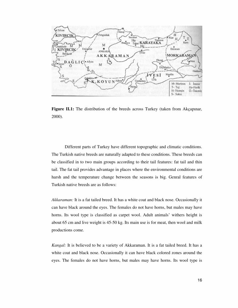
The distribution of the native sheep breeds of Turkey is given in the Figure
II.1 below. The most widely distributed breed is Akkaraman.
16
Figure II.1: The distribution of the breeds across Turkey (taken from Akçapınar,
2000).
Different parts of Turkey have different topographic and climatic conditions.
The Turkish native breeds are naturally adapted to these conditions. These breeds can
be classified in to two main groups according to their tail features: fat tail and thin
tail. The fat tail provides advantage in places where the environmental conditions are
harsh and the temperature change between the seasons is big. Genral features of
Turkish native breeds are as follows:
Akkaraman: It is a fat tailed breed. It has a white coat and black nose. Occasionally it
can have black around the eyes. The females do not have horns, but males may have
horns. Its wool type is classified as carpet wool. Adult animals’ withers height is
about 65 cm and live weight is 45-50 kg. Its main use is for meat, then wool and milk
productions come.
Kangal: It is believed to be a variety of Akkaraman. It is a fat tailed breed. It has a
white coat and black nose. Occasionally it can have black colored zones around the
eyes. The females do not have horns, but males may have horns. Its wool type is

17
classified as carpet wool. Adult animals’ withers height is about 85 cm and live
weight is 80 kg. Its main use is for meat, then wool and milk productions come.
Norduz: It is a fat tailed breed. It has a white coat color with some brown or grey
colored regions on it. There are black spots on head, neck and legs. Usually the ears
and eyes are in black, too. The females do not have horns, but males may have horns.
Its wool type is classified as carpet wool. Adult animals’ withers height is about 65-
70 cm and live weight is 45-55 kg. Its main use is for meat, then milk and wool
productions come.
Morkaraman: It is a fat tailed breed. It has a red or brownish coat color. The females
do not have horns, but males may have horns. Its wool type is classified as carpet
wool. Adult animals’ withers height is about 68 cm and live weight is 50-60 kg. Its
main use is for wool, then meat and milk productions come.
�vesi: It is a fat tailed breed. It has a white coat color with brown marks on feet, ears
and neck. The females do not have horns, but males do have horns. Its wool type is
classified as carpet wool. Adult animals’ withers height is about 65 cm and live
weight is 45-50 kg. Its main use is for milk, then meat and wool productions come.
Da�lıç: It is a fat tailed breed. It has a white coat color with occasional black marks
around mouth, nose and eyes. The females do not have horns, but males may have
horns. Its wool type is classified as carpet wool. Adult animals’ withers height is
about 58 cm and live weight is 35-40 kg. Its main use is for wool, then meat and milk
productions come.
Kıvırcık: It is a thin tailed breeds. It has a white coat color and may have black spots
on legs and face. The females may have horns, but males always have horns. Its wool
type is classified as carpet wool. Adult animals’ withers height is about 58 cm and
live weight is 35-40 kg. Its main use is for wool, then meat and milk productions
come.

18
Karayaka: It is a thin tailed breeds. It has a white coat color and black eyes, head and
legs. The females do not have horns, but males do have horns. Its wool type is
classified as carpet wool. Adult animals’ withers height is about 60-62 cm and live
weight is 35-40 kg. Its main use is for wool, then meat and milk productions come.
Hem�in: It is a thin tailed breeds with a fat deposition at the tail base. It has a mixed
coat color of white, brown and black. The females may have horns, but males always
have horns. Its wool type is classified as carpet wool. Adult animals’ withers height
is about 65 cm and live weight is 45-50 kg. Its main use is for meat, then wool and
milk productions come.
Konya Merinosu: It is a thin tailed crossbreed of German meat Merino (80%) and
Akkataman (20%). It has a white coat color. Adult animals’ withers height is about
66 cm and live weight is 54-56 kg. Its main use is for meat, then wool and milk
productions come.
Türkgeldi: It is a thin tailed crossbreed of East Friesian (9/16) and Kıvırcık (7/16), It
has a white coat color. It is found in Thrace, Turkey. They are a dairy breed also used
for meat and wool productions.
Hamdani: It is a fat tailed breed found in Iraq and Iran. It has a white coat color with
brown/black color on the face, ears and legs. Unfortunately, there is not much
information found in the literature about the breed characteristics of Hamdani.
There were two sampling strategies used during sample collection;
1. Some of the samples of the breeds were taken from governmental enterprises
or university farms. The names of the breeds and where they were taken from
are as follows: Akkaraman1 and Konya Merinosu breeds were sampled from
Konya Stud of Selçuk University, Konya; �vesi breed was sampled from
Gözlü Agricultural Enterprise, Konya; Türkgeldi breed was sampled from
Research and Application Unit of Trakya University in Tekirda� and Kıvırcık
breed was sampled from �nanlı Agricultural Enterprise, Tekirda�.

19
2. All the rest of the samples of the breeds, which are Da�lıç, Akkaraman,
Kangal, Karayaka, Hem�in, Morkaraman, Norduz and Hamdani, were
collected from local breeders and flocks. The flocks and the individuals to be
sampled were chosen with the help of veterinarians, veterinary technicians
and/or agricultural engineers so that morphologically the best representatives
of each breed were tried to be sampled. From each flock visited, 2-4 samples
were collected, considering the total size of the flock. By this way, the
maximum genetic variation within a breed was tried to be captured.
In table II.1 the names of the breeds and their repeated samples were given together
with the some details about these samples.
Table II.1. Description of the study material and sampling. FB: fat and big tail; FS:
fat and short tail; T: thin and long tail; FTB: thin tail which is fat at the base.
Breeds Abbrev. Sample
size Breeding Farm
(B)/Flock (F) Native (N)/ Foreign (F)
Pure (P)/ Crossbreed (C)
Tail type
Akkaraman Akk 52 B and F N P FB Akkaraman1 Akk1 28 B N P FB Akkaraman2 Akk2 10 F N P FB Akkaraman3 Akk3 14 B and F N P FB �vesi �ve 35 B N P FB Kıvırcık Kıv 23 B N P T Morkaraman Mork 35 F N P FB Hem�in Hem 34 F N P FTB Karayaka Kry 57 F N P T Karayaka1 Kry1 28 F N P T Karayaka2 Kry2 29 F N P T Da�lıç Da� 64 F N P FS Da�lıç1 Da�1 32 F N P FS Da�lıç2 Da�2 32 F N P FS Norduz Nor 26 F N P FB Kangal Kngl 22 F N P FB Hamdani Ham 22 F F P FB Konya Merinosu KM 29 B N C FS Türkgeldi TG 24 B N C T

20
During sample collection as many places as possible visited for each breed.
The area covered during sampling is shown in Figure II.2. Details about the
addresses of the sampling places were given in Appendix A where possible.
Figure II.2. Sampling locations. The dashed lines discriminate between the
distribution areas of the breeds and the area covered during sampling was shadowed.
The names of the sampled breeds and the names of the cities within the sampling
area are given. Underlined breeds are from governmental and university farms.
II.2. DNA Isolation
Standard phenol: chloroform DNA extraction protocol (Sambrook et al.,
1989) was used for extracting DNA from the blood samples collected. All the DNAs
were extracted at Middle East Technical University, Department of Biology.

21
10 ml of blood sample was put in 0.5 ml EDTA (0.5 M; pH 8.0) containing
falcon tube and 2X lysis buffer (10X Lysis solusyonu: 770 mM NH4Cl, 46 mM
KHCO3, 10mM EDTA) was added onto it until the volume was 50 ml. After mixing
the content of the tube well by inversions for 10 min. the tubes were centrifuged at
3000 rpm at +4°C for 10 min. The supernatant was poured off and 3 ml of
salt/EDTA (75mM NaCl, 25 mM EDTA) was added onto the pellet and mixed by
vortex. After the addition of 0.3 ml of %10 SDS solution and 150 µl of proteinase K
(10 mg/ml) solution, the samples were incubated at 55°C for 1-3 hr. When the time is
over, 3 ml of phenol (pH 8.0) was added on to the samples, the tubes were shaken
vigorously for 20 s and then by gentle inversions for 5 min. Afterwards, the tubes
were centrifuged at 3000 rpm at +4°C for 10 min. The supernatant was transferred
into new sterile tubes labeled properly and 3 ml of phenol:cloroform:isoamyl alcohol
(25:24:1) was added on to the supernatant, which was then shaken vigorously for 20
s and then by gentle inversions for 5 min. Moreover, the tubes were centrifuged at
3000 rpm at +4°C for 10 min for the last time and the supernatant was transferred
into a sterile glass tube, to which 2 volumes of ice cold. (kept at –20°C) EtOH was
added. The glass tubes were shaken abruptly, the condensed DNA was hooked out
with a glass hook and transferred in to 1.5 ml eppendorf tubes containing 0.5 ml of
TE buffer (10mM Tris, 1mM EDTA PH 7.5). The DNA solution can be either stored
at +4°C (if it is going to be used immediately) or at -20°C (for long term storage).
II.3. Microsatellite Used
Five microsatellite loci have been chosen for this study after consulting with
Prof. Mike Bruford from Cardiff University, Dr. Kate Byrne from London Institute
of Zoology and FAO webpage (http://dad.fao.org/en/refer/library/guidelin/
marker_without_link.pdf). They were chosen because they were all polymorphic, a
data from European samples were available, and data are accumulating based on
these loci. The names of these microsatellite loci, their origin, on which chromosome
they are located and their allelic range were given in Table II.2 below.

22
Table II.2. Microsatellite markers used in the study; their names, origins,
chromosome numbers and allelic ranges.
Locus Origin Chromosome
# Allelic Range
MAF33 Ovine 9 122-154 MAF65 Ovine 15 117-139 MAF209 Ovine 17 104-136 JMP29 Ovine 24 115-155 JMP58 Ovine 26 140-176
II.4. Polimerase Chain Reaction (PCR) Conditions
All the DNA samples were amplified with the primers specific to these five
microsatellite loci by using Biometra, Stratagene and Perkin Elmer 3700 Polymerase
Chain Reaction (PCR) machines.
The amplified products were either visualized by radioactive labeling using 33P dATP (for the samples analyze at Middle East Technical University, Department
of Biology) or by fluorescent labeling using FAM, TET and HEX flourophores (for
the samples analyzed at Cardiff University, School of Biosciences).
• For radioactive labeling, 1X PCR mixture contained 1X PCR buffer, 2.5 mM
MgCl2; 200mM of dTTP, dCTP and dGTP; 20 mM of dATP; 0.1 µl of
1000mCi 33P dATP; primers of the locus to be amplified and sterile distilled
water to adjust the volume. The primer concentrations used in the 1X PCR
master mix are as follows; 6 pmol from each of forward and reverse MAF 33
primers, 4 pmol from each of forward and reverse MAF 65 primers, 5 pmol
from each of forward and reverse MAF 209 primers, 7 pmol from each of
forward and reverse JMP29 and JMP58 primers. This mixture was distributed
to PCR tubes containing 50-100 ng DNA samples and then 1 unit of Taq
DNA polymerase was added into each tube and the tubes were placed in PCR
machine for amplification.

23
• For fluorescent labeling, 1X PCR mixture contained 1X PCR buffer, 2.5 mM
MgCl2; 200mM of each of dNTP; primers of the locus to be amplified and
sterile distilled water to adjust the volume. The primer concentration used
was the same, but the primers were fluorescently labeled. Similar to
radioactive labeling the mixture was distributed to PCR tubes containing 50-
100 ng DNA samples and then 1 unit of Taq DNA polymerase was added
into each tube and the tubes were placed in PCR machine for amplification.
The PCR amplification conditions are as follows: 1 cycle of denaturation at
94°C for 2 min; 30 cycles of amplification process where the samples are incubated
at 94°C for 20 s, then at the annealing temperature specific for the primers for 20 s,
and then at 72°C for 40 s; 1 cycle of final extension at 72°C for 10 min. The
annealing temperatures of the loci used in the study are 57°C for MAF33, MAF65,
JMP29 and JMP58 loci, and 60°C for MAF209 locus.
The PCR products were checked on 1.5% agarose gels for amplification.
II.5. Polyacrylamide Gel Electrophoresis and Data Collection
There were two methods used for polyacrylamide gel electrophoresis as there
were two labeling methods used:
• For radioactive labeling (used for the samples analyzed at Middle East
Technical University, Department of Biology); 6X loading dye (with
formamide) was added to the PCR products, and then they were kept at 95°C
for 3 min for denaturation and kept on ice for loading. Then 3 µl of samples
were loaded onto 6% denaturing polyacrylamide gel. After running the gel
for 2-4 hr at 1600V, the glass plates were separated. As Sigmacote was
applied to the back plate, the gel was only sticked to the front plate. Then the
gel is transferred carefully on to 3M whatman paper and stretch film is placed
on the gel. Afterwards, the gel was dried in vacuum gel dryer at 60°C for
about an hour. Finally the gel was placed in exposure cassette and radioactive
sensitive film was placed on it properly. According to the radioactive labeled

24
dNTP's delivery date the film was exposed to the gel for 3 days to 15 days
before it was washed.
• For fluorescent labeling (used for the samples analyzed at Cardiff University,
School of Biosciences); 1.5 µl of each PCR product were mixed with 1.2 µl
of Tamra350 internal size standard (labelled with red colour). After
incubating the mixture at 95°C for 3 min. samples were loaded onto 4.2%
non-denaturing polyacrylamide gel in an ABI 377 semi-automated DNA
analyzer. The raw data were collected by GeneScan software of Perkin
Elmer. After the data is collected, electrophenograms of the amplified alleles
were checked and the allelic sizes were determined in comparison with the
internal size standard by using Genotyper software of Perkin Elmer.
II.6. Data Analysis
The first collected samples were from the governmental and university farms
(Akkaraman1, Kıvırcık, �vesi, Konya Merinosu, Türkgeldi). Right after completion
of the data from these breeds the results were tested for the presence of close
relatives within the sample and some of the individuals from each of the 5 samples
were excluded using the software Kinship (Goodnight and Queller, 1999).
After completion of the data collection, data matrix file was constructed so
that it could be analyzed using GENETIX 4.02 software (Belkhir et al. 1996-2004)
which is available at the website: http://www.univ-montp2.fr/~genetix/genetix.htm.
This program computes several basic parameters of sample genetics such as Nei's D
and H, Wright's F-statistics (using the Weir-Cockerham's and Robertson-Hill's
estimators). For each of them, the distribution of the parameter values under the null
hypothesis is generated by the appropriate resampling scheme of the relevant objects
(e.g. alleles between individuals in the case of FIS) using permutations. The
permutation-based statistical inference procedures implemented in GENETIX
estimates the probability value of departure from the null hypothesis.

25
In addition, GENETIX file format was used in further analyses performed by
using the softwares Geneclass (Cornuet et al., 1999) for the assignment tests,
Bottleneck (Cornuet and Luikart, 1996) for the analysis of the probability of a recent
reduction in the sample size. Furthermore GENETIX program converts the data file
into the GENEPOP file format, which was used in Populations 1.0 software
(http://www.cnrs-gif.fr/pge/bioinfo/samples) to construct the neighbour-joining trees
based on the DA genetic distance between samples and the proportion of shared
alleles between the individuals, and into the Arlequin (Excoffier et .al., 1992) file
format, which was used for Mantel Test, AMOVA and FST estimations. Furthermore,
the allele frequencies used for Principle Component analysis performed by
NTSYSpc (www.exetersoftware.com/cat/ntsyspc/ntsyspc).
II.6.1 Kinship Analysis
In Turkey, pedigree records are not taken in sheep breeding. Therefore, the
relationship between the individuals of each of the five breeds (Akkaraman1,
Kıvırcık, �vesi, Türkgeldi and Konya Merinosu), which are taken from the
governmental enterprises and the university breeding farms, is not known. There may
be close relatives within the same sample, which in turn will affect the results of the
statistical analyses. Therefore, after completing the data collection from these five
breeds, the results were first tested for relatedness and parentage probabilities by
using the software Kinship (Goodnight and Queller, 1999; see the webpage at
http://www.gsoftnet.us/GSoft.html). It performs maximum likelihood tests of
pedigree relationships between pairs of individuals in a population based on the
genotype information for single-locus, codominant genetic markers (e.g.
microsatelites). The user enters two hypothetical pedigree relationships, a primary
hypothesis and a null hypothesis. Then, the program estimates likelihood ratios
comparing the two hypotheses for all possible pairs in the data set. In addition, it
generates simulated data sets from the given genetic data to test the significance of
results. Moreover, it estimates pairwise relatedness statistics. The resulting file is a
matrix showing the likelihood ratio between primary and null hypotheses.
26
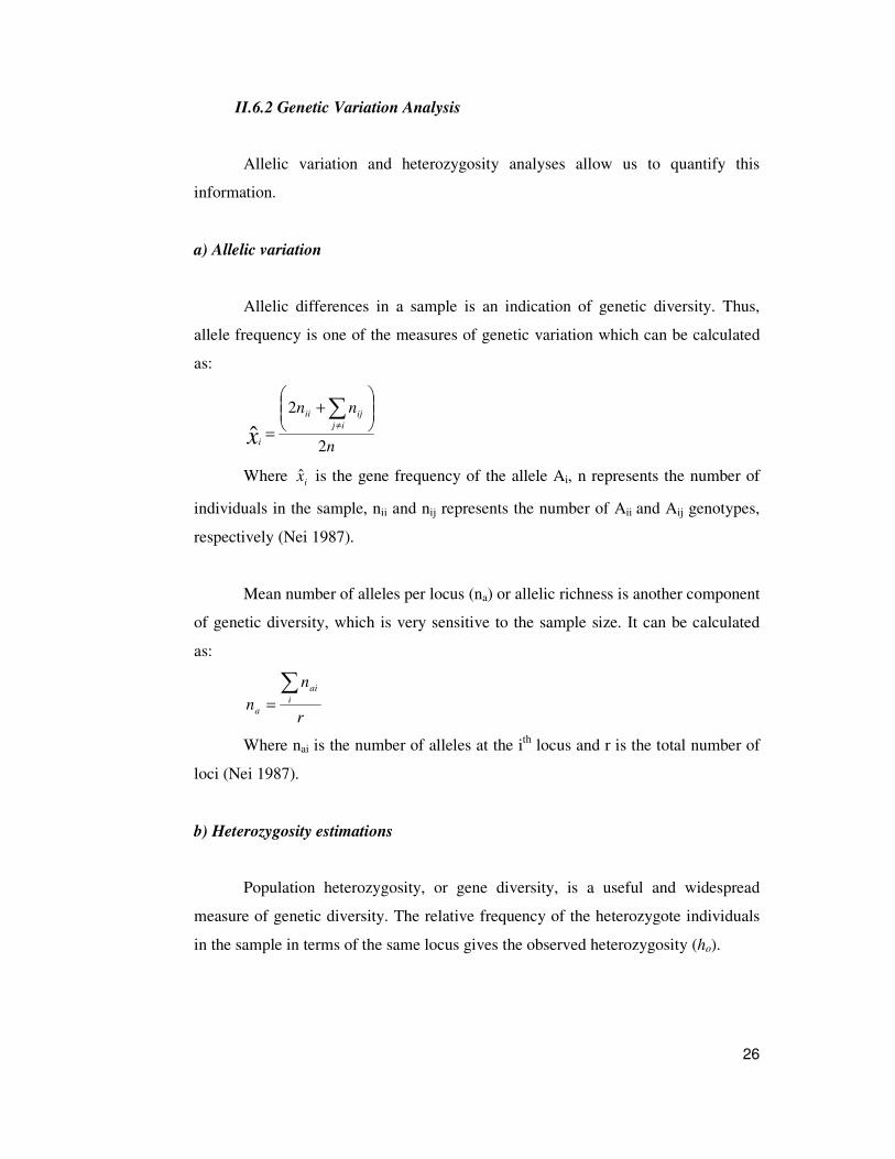
II.6.2 Genetic Variation Analysis
Allelic variation and heterozygosity analyses allow us to quantify this
information.
a) Allelic variation
Allelic differences in a sample is an indication of genetic diversity. Thus,
allele frequency is one of the measures of genetic variation which can be calculated
as:
n
nnij
ijii
ix 2
2
ˆ���
����
�+
=�
≠
Where ix is the gene frequency of the allele Ai, n represents the number of
individuals in the sample, nii and nij represents the number of Aii and Aij genotypes,
respectively (Nei 1987).
Mean number of alleles per locus (na) or allelic richness is another component
of genetic diversity, which is very sensitive to the sample size. It can be calculated
as:
r
nn i
ai
a
�=
Where nai is the number of alleles at the ith locus and r is the total number of
loci (Nei 1987).
b) Heterozygosity estimations
Population heterozygosity, or gene diversity, is a useful and widespread
measure of genetic diversity. The relative frequency of the heterozygote individuals
in the sample in terms of the same locus gives the observed heterozygosity (ho).

27
Nei (1987) formulated the unbiased estimate of the expected heterozygosity,
or gene diversity, which eliminates the bias that may result from sample size. The
expected heterozygosity ( eh ) at a locus can be estimated by the formula:
( )( )12
ˆ12ˆ2
−−
= �n
xnh i
e
Where n is the number of individuals and ix is the frequency of the allele Ai (Nei,
1987).
In case of multi loci, the average of single locus heterozygosity values is
taken to find sample's observed (HO) and expected (HE) heterozygosities.
II.6.3. F-statistics
In actual sample, the genotype frequencies in each subpopulation do not
necessarily follow Hardy-Weinberg equilibrium. Wright's fixation indices FIS, FIT
and FST measure the deviations from Hardy-Weinberg expectations in terms of
genotype frequencies in a subdivided sample. These coefficients are used to allocate
the genetic variability to the total sample level (T), samples (S) and individuals (I),
and they are useful to understand the breeding structure of the sample.
These three F-coefficients are interrelated so that;
( )( )ISSTIT FFF −−=− 111 or IS
ISITST F
FFF
−−
=1
Nei (1987) showed that FIS, FIT and FST can be defined in terms of expected and
observed heterozygosities and still satisfies the above equation.
FIS is defined as the correlation between homologous alleles within
individuals relative to the samples. It deals with the inbreeding in induviduals at the
subpopulation level so that it measures the deviation from the Hardy-Weinberg
equilibrium within the samples. It is estimated by the following formula:
S
OSIS H
HHF
−=

28
FIT is defined as the correlation of the corresponding alleles within
individuals relative to the total sample and it accounts for both the effects of
inbreeding within samples and the effects of sample subdivision. FIT quantity
measures the deviation from Hardy-Weinberg equilibrium over the total sample. The
following formula estimates FIT:
T
OTIT H
HHF
−=
FST is a measure of genetic differentiation of samples. It deals with inbreeding
in samples relative to the total sample and it can be estimated by the following
formula:
T
STST H
HHF −=
Where;
HO = average observed heterozygosity of the samples
HS = average expected heterozygosity in the samples
HT = average heterozygosity of the total sample
(Hedrick, 1983; Nei 1987, Nei and Kumar, 2000)
The F indices proposed by Wright (1951) does not consider the unequal finite
sample sizes and there is some disagreement on the interpretation of the quantities
and on the method of evaluating them. Weir and Cockerham (1984) revised the F
coefficients in order to offer some unity to various estimation formulae suggested by
different authors. They used the parameters F, � and f for FIT, FST and FIS
respectively. These estimators do not make assumptions concerning numbers of
samples, sample sizes or heterozygote frequencies and they are suited to small data
sets. F, � and f parameters are estimated as follows:
)/(1)/()/(1
CBACf
CBAA
CBCF
++−=++=+−=
θ
Where;
A=inter-sample component of allelic frequency variance

29
B=component of allelic frequencies variance between individuals in each
sample
C=component of allelic frequencies variance between gametes in each
individual
In this study, Weir and Cockerham's approach is used to examine the sample
structure, but the parameters are denoted by FIT, FST and FIS instead of F, � and f.
In order to test the significance of estimated F-coefficients, the data were
permuted for 1000 times and the distribution of the calculated values (FIS and FST)
from the permuted data was generated under the null hypothesis (no sample
differentiation for FST, and HW equilibrium for FIS and FIT). The probability of
obtaining original estimated F-coefficients under the null hypothesis was calculated
as the proportion of the distribution having values larger than the original value. For
FIS, alleles were permuted within each sample whereas for FST, genotypes were
permuted among the samples.
II.6.4. Anaysis of Molecular Variance (AMOVA)
With the new advances in molecular genetic techniques and the new devices
developed, it is easier to collect information on allele frequencies, as well as on the
amount of differences (mutations) between alleles. When studying molecular
variation, haplotypic data should be used so that there is no variation within
individuals. Analysis of Variance (ANOVA) compares average gene frequencies
among samples. That is why, Excoffier and his collaborators (1992) modified
ANOVA analysis to incorporate the molecular information in it and named it as
AMOVA (Analysis of Molecular Variance). A variety of molecular data – molecular
marker data (for example, RFLP or AFLP), direct sequence data, or phylogenetic
trees based on such molecular data – may be analyzed using this method (Excoffier,
et al. 1992).

30
Analysis of Molecular Variance (AMOVA) is a method for studying
molecular variation within a species and the results are tested. It estimates the
partitioning of total genetic variation;
• Among groups of populations,
• Among the populations within groups,
• Among the individuals within a population.
The raw molecular data is treated as a Boolean vector pi in AMOVA. The
data are converted in to a 1xn matrix of 1s and 0s, 1 indicating the presence of a
marker (1) and its absence (0). Then AMOVA is performed using Euclidean
distances derived from vectors of 1s and 0s, which is unlikely to follow a normal
distribution. A null distribution is therefore computed by resampling of the data
(Excoffier, et al. 1992). In each permutation, each individual is assigned to a
randomly chosen population while holding the sample sizes constant. These
permutations are repeated many times, eventually building a null distribution.
Hypothesis testing is carried out relative to these resampling distributions.
There are some assumptions included in AMOVA (Excoffier, et al. 1992):
The individuals from which haplotypes are sampled should be chosen independently
and at random, or coarse. The mating in the sampled population is entirely random
and non-assortative and no inbreeding occurs. Thus, if non-random mating or
inbreeding is occurring, it will result in lower heterozygosity, and if the rates of non-
random mating or inbreeding differ between populations, fixation estimates will be
confounded.

31
The AMOVA design and the formulae are given below;
--------------------------------------------------------------------
Source of sum of mean Expected mean Variation d.f. squares squares squares --------------------------------------------------------------------
Among groups G-1 SS(AG) 1
)(−GAGSS
222a
mb
nw nn σσσ ++
Within groups
among samples d-G SS(AD) Gd
ADSS−
)( 2'2
bw n σσ +
Within samples n-d SS(WD) dn
WDSS−
)( 2
wσ
--------------------------------------------------------------------
Total n-1 SS(T) --------------------------------------------------------------------
� �= n
i
n
j ijnTSS 2
21
)( δ
� � � � �×−= G
g
d
k
d
k
n
i
n
j ijg
gk gk
nTSSAGSS
'
2
21
)()( δ
� � � � � −×= G
g
d
k
d
k
n
i
n
j ijg
g g gk gk WDSSn
ADSS'
2 )(2
1)( δ
� � � �×= G
g
d
k
n
i
n
j ijgk
g gk gk
nWDSS 2
21
)( δ
g
G
gdd �=
� �= G
g
d
k gkg nn
�= gd
k gkg nn

32
� �� � = == =−= G
g
d
k gkg
G
g
d
k gkgg n
nn
dn
1 12
1 1
11'
� �� � = == =−
−= G
g
d
k gk
G
g
d
k gkgg nn
Gn
1 12
1 12
11
''
( )2
1 1
11
1''' � �= =
−−
= G
g
d
k gkg n
nn
Gn
In this study AMOVA analysis was employed to analyze how the total
genetic variation was partitioned within and among breeds (for similar application,
see Tserenbataa et al., 2004).
II.6.5. Genetic Distance Estimations and Tree Construction
The distance matrix approaches used in this study are as follows:
(i) Nei's DA Genetic Distance
The DA genetic distance is considered as the most appropriate method to
obtain correct tree topology from microsatellite data (Takezaki and Nei, 1996). It is
based on infinite allele model and calculated as:
� �−= r
j
m
i ijijAj yx
rD
11
Where xij and yij are the frequencies of the ith allele at the jth locus in samples X and
Y, respectively and mj is the number of alleles at the jth locus, and r is the number of
loci examined.
(ii) Allele Sharing Distance
This method is based on the idea that alleles which are common in all
samples of the same species are likely to have existed before the split of these

33
samples; so that they might also be more frequent than the newly formed ones that
might not shared by all. As a result, the proportion of shared alleles increases with
increasing genetic similarity of the samples.
Shared allele distance between individuals (DSAi) is calculated as follows:
DSAi = 1 - PS with r
SPS 2
�=
where the number of shared alleles (S) is summed over all loci, r (Chakraborty et al.
1992, Bowcock et al. 1994).
Phylogenetic tree construction method used:
Neigbor Joining (NJ) tree construction method is a distance based approach
which aims to minimize the total length of tree by sequentially finding the neighbors.
This method is used rather than UPGMA, which is another distance based approach,
because NJ does cluster analysis allowing for unequal rates of molecular change
among branches (Avise, 1994). Also, the comparative studies among different tree
construction methods have suggested that NJ method performs better than the others
under nonuniform rates either among lineages or among sites (Saitou and Nei, 1987;
Li, 1997).
II.6.6. Factorial Correspondance Analysis (FCA)
The Factorial Correspondence Analysis (FCA) is performed to visualize the
individuals in multidimensional space and to explore the relationships between the
individuals. It involves a linear transformation of the number of alleles at each locus
for each individual, which can have 0, 1 or 2 copies of an allele at a particular locus.
The coefficients are chosen to maximize the variation of the transformed data
measured along each coordinate axis. The first three axes are the most informative
ones (MacHugh et al., 1997; Byrne et al., in press). As a result, it is possible to
visualise how the individuals are related to each other on the independent axis
chosen.

34
II.6.7. Assignment Test
Assignment tests were performed to test if the data on the five microsatelite
loci chosen for the study provide enough genetic information to assign individual
samples only to their original breeds. There are two types of methods for assigning
individuals to samples: (i) likelihood-based methods in which individuals are
assigned to the sample where the likelihood of their genotype is highest and (ii)
genetic distance-based methods in which individuals are assigned to the (genetically)
closest sample.
In addition, every assignment method can be used in two different ways. In
the first way, noted "direct" in the interface, the chosen criterion (likelihood or
genetic distance) is used directly to assign the individual. In the second way, noted
"simulation", a "probability" that the individual belongs to each sample is computed.
It can be used to exclude samples as origins of individuals.
In this study, Bayesian type likelihood method is used to assign the
individuals by simulating them 10000 times per samples. Also 5 different probability
criteria to reject the assignment of the individual to the sample of interest were used,
which are P<0.001, P<0.01, P<0.05, P<0.2, and P<0.5.
II.6.8. Principal Component (PC) Anaysis
By definition, principle components are a set of variables that define a
projection that encapsulates the maximum amount of variation in a dataset and is
orthogonal (and therefore uncorrelated) to the previous principle component of the
same dataset. Principle Component (PC) analysis is designed to capture the variance
in a dataset in terms of principle components. In this analysis, individuals cannot be
shown. A sample is represented as a single point in space constructed by PCs
In the vector space, PC analysis identifies the major directions and the
corresponding strengths of the variation in the data. PC analysis achieves this by
computing the eigenvectors and eigenvalues of the covariance matrix of the data.

35
Keeping only a few eigenvectors corresponding to the largest eigenvalues, PC
analysis can also reduce the dimensions of the data while retaining the major
variation of the data.
For the PC analysis analysis, NTSYSpc software was used (Exeter software;
www.exetersoftware.com/cat/ntsyspc/ntsyspc).
II.6.9. Delaunay Network Analysis
Delaunay network is performed, by applying Thiessian polygons on the study
area (Monmonier, 1973). First the map of the study area is taken and divided into
regions. In this case the regions are the distribution areas of the studied breeds. Then
points are placed in the center of the regions as representatives of the regions or
breeds. Afterwards, the outer boundary of the study area is drawn with joining the
points at the outer regions. The next step is to join all the interior points based on
"shortest distance" criterion to form triangles. The resulting figure is called
"Delaunay Network".
In order to find about the possible genetic barriers pairwise genetic
differences between the breeds are written on the corresponding edges of the
triangles joining the points (Brassel and Reif, 1979). A perpendicular is drawn to the
one of the triangle edges in the outer boundary, which has the highest pairwise
genetic distance. Then the perpendicular line is directed towards the one of the
remaining two edges of that triangle, which has the highest pairwise genetic distance
and you are either in the neighboring triangle or outside of the outer polygon.
Drawing of the perpendicular lines is continued until you are outside of the polygon,
which is considered as a barrier. The drawing of the second barrier is started from
one of the edges of the outer polygon, which is untouched by the first barrier and has
the highest pairwise genetic distance than the rest of the untouched edges of the
polygon. Drawing of the second barrier continues till it meets the first barrier or it
goes out of the polygon. The drawing of the barriers continues until all the edges of
the outer polygon are tested. If the barrier does not go out of the polygon, but drive

36
circles inside it, then it means there is no barrier. The order with which the barriers
are drawn also means as the order of their priority.
II.6.10. Mantel Test
The principle of mantel test is to test the presence of correlation between two
distance matrices (Mantel, 1967; Rousset and Raymond, 1997). For example, the
relation between genetic distance matrix and geographic distance matrix can be
tested for the presence of isolation by distance. Using proper statistics, it is not only
possible to investigate the relationship between the elements of two matrices but also
it is possible to test the statistical significance of the results by permutation test.
II.6.11. Bottleneck Analysis
This analyis is used to investigate the probability for the occurence of a recent
bottleneck in the sample of interest. The software, named as Bottleneck, used for this
test is based on the hypothesis that the allelic diversity (HE) is reduced faster than the
heterozygosity (HO) if samples experience a recent reduction of their effective
sample size.
In order to detect recent effective sample size reductions, the program
Bottleneck uses the allelic frequencies and it computes for each sample sample and
for each locus the distribution of the heterozygosity expected from the observed
number of alleles (k), given the sample size (n) under the assumption of mutation-
drift equilibrium. This distribution is obtained through simulating the coalescent
process of n genes under three possible mutation models, the IAM (Infinite allele
model), TPM (Two-phased model, both IAM and SMM in different percentages used
in simulation) and the SMM (Stepwise mutation model) using either genetic distance
or bayesian approaches. This enables the computation of the average (Hexp), which is
compared to the observed heterozygosity to establish whether there is a
heterozygosity excess or deficit at this locus. In addition, the standard deviation (SD)
of the mutation-drift equilibrium distribution of the heterozygosity is used to

37
compute the standardized difference for each locus ((HO-HE)/SD). The distribution
obtained through simulation enables also the computation of a P-value for the
observed heterozygosity.
Once all loci available in a sample sample have been processed, the three
statistical tests (sign test, Wilcoxon test and standardized differences test) are
performed for each mutation model and the allele frequency distribution is
established in order to see whether it is approximately L-shaped (as expected under
mutation-drift equilibrium) or not (recent bottlenecks provoke a mode shift).
In this study, TPM was employed with bayesian approach and Wilcoxon test
(as recommended by the authors for microsatellite data) was used to test the
significance of the results after permuting the data 1000 times (see Cornuet and
Luikart, 1996 for details).
II.6.12. List of Statistical Analysis Methods Applied and the Softwares Used
The summary list of the statistical methods used in data analysis of these
study and the names of the softwares used to perform these statistical test are given
(in paranthesis) below:
• Exclusion of one of the relatives (Kinship 1.1)
• Allelic diversity and gene diversity estimations (Genetix 4.02)
• F statistics (Genetix 4.02, Arlequin 2.001)
• Analysis of Molecular Variance (Arlequin 2.001)
• Genetic distance estimations and NJ tree construction (Populations)
• Factorial Correspondence Analysis (Genetix 4.02)
• Assignment Test (GeneClass)
• Principle Component Analysis (NTSYSpc)
• Delaunay Network for construction of genetic barriers
• Mantel Test (Arlequin 2.001)
• Bottleneck Test (Bottleneck)

38
The webpage addresses for these softwares are:
• Kinship 1.3.1. : http://www.gsoftnet.us/GSoft.html
• Genetix 4.02 : http://www.univ-montp2.fr/~genetix/genetix.htm
• Arlequin 2.001 : http://anthropologie.unige.ch/arlequin/
• Populations : http://www.pge.cnrs-gif.fr/bioinfo/wini386/samples.exe
• GeneClass : http://www.ensam.inra.fr/URLB/
• NTSYSpc : http://www.exetersoftware.com/cat/ ntsyspc/ntsyspc
• Bottleneck : http://www.ensam.inra.fr/URLB/

39
���������
RESULTS
In this chapter first the results of the analyzed data will be presented. The
allelic data collected for this study were given in the Appendix B. This data were
analyzed by all the statistical methods explained in the previous chapter.
III.1. Kinship
Before analyzing all the data, first, the samples collected from breeding farms
were tested for relatedness and some individuals were discarded as they were closely
related to some of the individuals in the same sample collected from governmental
and university farms (which are Akkaraman1, Kıvırcık, �vesi, Konya Merinosu and
Türkgeldi). The initial population sizes of each of the 5 samples were 35. After
excluding the relatives and some samples that did not amplify for all the five loci, the
sample sizes (n) for Akkaraman1, Kıvırcık, �vesi, Konya Merinosu and Türkgeldi
became 28, 23, 35, 29 and 24, respectively. For this exclusion process, the results of
the kinship analysis were used and the criteria there in (Goodnight and Queller,
1999).

40
III.2. Allelic Variation
The total number of alleles observed for the loci used in the study is given in
Table III.1 below. The highest and the lowest number of alleles observed for single
locus is 21 for JMP29 and 11 for MAF 33, respectively. The number of alleles
observed for each locus in each breed and the average numbers were given in Table
III.2.
Table III.1. Total number of observed alleles for the loci employed in the study.
Locus Name
Observed Number of
Alleles MAF33 11 MAF65 13 MAF209 15 JMP29 21 JMP58 18

41
Table III.2. Total number of alleles observed for each locus in each breed and
sample, the mean number of alleles observed for each breed/sample (MNA/pop) and
for each locus (MNA/locus)
MAF33 MAF65 MAF209 JMP29 JMP58 MNA/pop Akkaraman 6 7 10 14 13 10 Akkaraman1 4 5 8 10 10 7.4 Akkaraman2 4 5 3 9 8 5.8 Akkaraman3 6 6 5 10 9 7.2 �vesi 7 8 9 11 11 9.2 Kıvırcık 8 6 7 9 10 8 Morkaraman 9 9 10 12 9 9.8 Hem�in 8 8 9 8 10 8.6 Karayaka 10 9 8 14 16 11.4 Karayaka1 10 8 8 12 14 10.4 Karayaka2 7 8 6 11 14 9.2 Da�lıç 9 9 10 12 13 10.6 Da�lıç1 6 7 8 10 11 8.4 Da�lıç2 8 9 9 12 11 9.8 Norduz 8 8 7 12 9 8.8 Kangal 7 7 8 11 9 8.4 Hamdani 5 7 9 7 6 6.8 Konya Merinosu 4 4 7 8 11 6.8 Türkgeldi 5 5 7 7 5 5.8 MNA/locus 6.6 6.9 7.5 9.9 9.8 8.2
The highest and lowest mean numbers of observed alleles per locus were 9.9
(JMP29) and 6.6 (MAF 33), respectively. The highest and the lowest observed mean
numbers of alleles per sample were 10.4 (Karayaka1) and 5.8 (Türkgeldi and
Akkaraman2), respectively. The observed mean number of alleles per sample is
greater than 8 for all the samples of the study except for Akkaraman1, Hamdani,
Konya Merinosu and Türkgeldi. Moreover, the mean number of alleles observed in
the study per locus per sample is 8.4.
When the frequencies of the observed alleles were examined, given in
Appendix C, it was determined that some of the alleles were present only in one of

42
the breeds. These alleles are called as breed specific or private alleles. The names of
both the loci and the breeds for which the private alleles were observed, and the
number of private alleles are given in the Table III.3.
Table III.3. The distribution of private alleles observed in the study and their
frequencies. Two alleles with highest frequencies were shown in bold.
Locus Allele Frequency Sample found
113 0.010 Akkaraman1 119 0.009 Karayaka1 153 0.026 Karyaka1
JMP29
159 0.023 Kıvırcık 134 0.018 Karayaka1 138 0.456 Kıvırcık JMP58 146 0.009 Karayaka2 109 0.023 Kangal MAF65 119 0.038 Norduz 108 0.023 Kangal 110 0.273 Kıvırcık MAF209 136 0.015 Morkaraman
In total, 12 such alleles were observed. The highest number of private alleles
(4) was found in JMP29, which also has the highest number of alleles and the highest
mean number of alleles observed per locus. There are no private alleles found in
MAF33, which has the lowest number of alleles observed. There are 2 private alleles
observed for MAF65 locus and 3 private alleles in both MAF209 and JMP58 loci.
Kıvırcık and Karayaka1 samples have 3 private alleles each; Kangal has 2;
Karayaka2, Akkaraman1, Morkaraman and Norduz have 1 private allele. In general,
these private alleles are found at either end of the allelic range with a low frequency
(between 0.01 and 0.05). As their frequencies are quite low, they cannot be used as in
identification of the breeds. However, two private alleles observed in Kıvırcık breed
are significant due to their high frequencies, which are allele-110 of MAF209 locus
(frequency: 0.27) and allele-138 of JMP58 locus (frequency: 0.46).

43
In order to visualize the alleles observed for each breed and their frequencies
frequency distribution histograms were constructed and given in the Appendix D.
Alleles 124 and 136 are the most common alleles observed in MAF33 locus in the
samples analyzed. Alleles 127, 129 and 131 are the most common ones observed in
MAF65 locus in general. In MAF 209 locus, allele-118 is the most common allele
observed with high frequency (0.2-0.5) in all of the breeds except for Kıvırcık in
which allele-110 (confined to Kıvırcık) and allele-112 have the highest frequencies
and the frequency of allele-118 is lower than 0.1. The most common alleles of
JMP29 locus are 135, 137 and 139. Finally, alleles 142 and/or 144 are the two most
common alleles observed in all breeds except for Kıvırcık in which allele 138
(Confined to Kıvırcık) has the highest frequency and both 142 and 144 have
frequencies lower than 0.1.
The frequency distribution graphs of alleles (Appendix D) observed for each
breed were placed on a map with respect to the distribution of the breeds across
Turkey in order to see if there is a particular pattern (e.g. West-East, North-South;
Northeast-Southwest or Southeast-Northwest) in the distribution of the alleles. This
was repeated for each locus analyzed and the graphs are given in Figure III.1 – III.5.

44
Figure III.1. The allele frequency distribution charts of MAF33 alleles for Turkish
native breeds and Hamdani placed on map of Turkey.
Figure III.2. The allele frequency distribution charts of MAF65 alleles for Turkish
native breeds and Hamdani placed on map of Turkey.
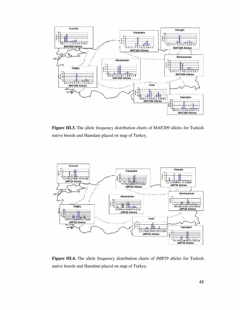
45
Figure III.3. The allele frequency distribution charts of MAF209 alleles for Turkish
native breeds and Hamdani placed on map of Turkey.
Figure III.4. The allele frequency distribution charts of JMP29 alleles for Turkish
native breeds and Hamdani placed on map of Turkey.
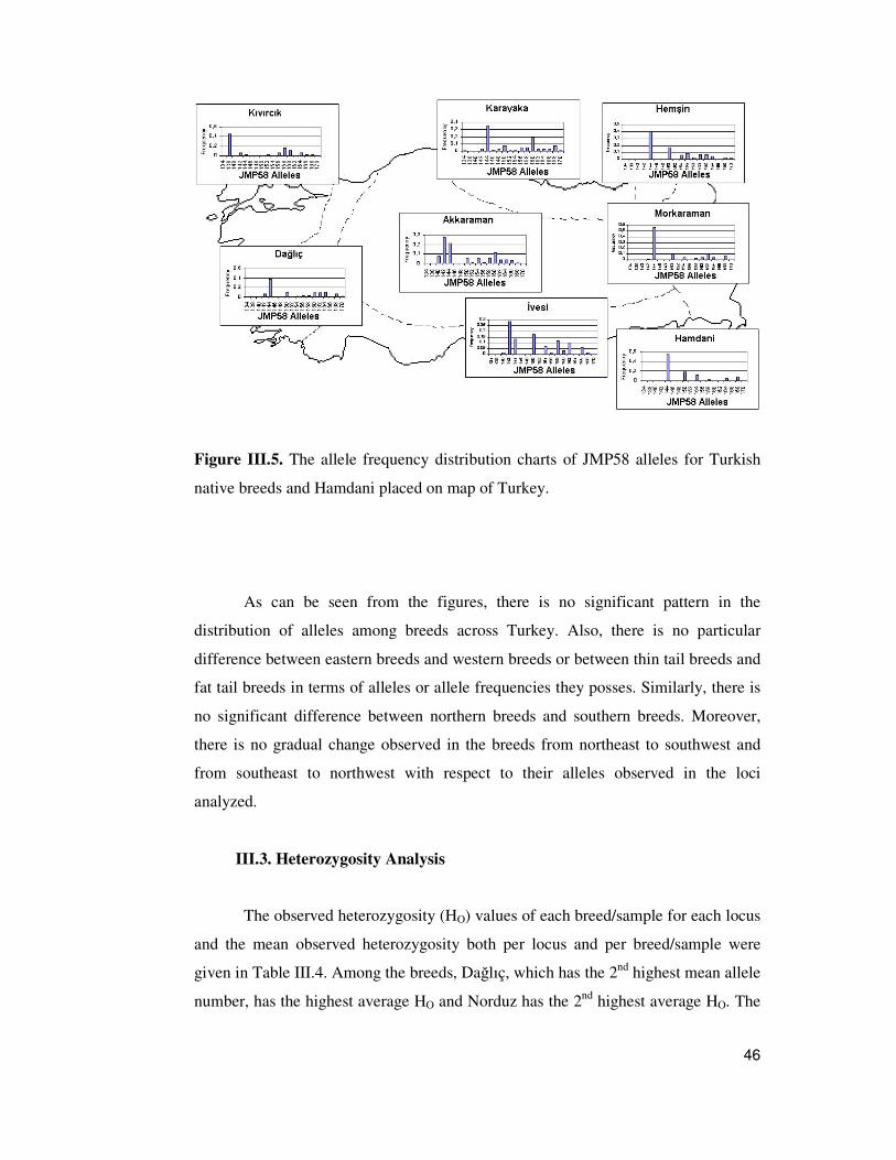
46
Figure III.5. The allele frequency distribution charts of JMP58 alleles for Turkish
native breeds and Hamdani placed on map of Turkey.
As can be seen from the figures, there is no significant pattern in the
distribution of alleles among breeds across Turkey. Also, there is no particular
difference between eastern breeds and western breeds or between thin tail breeds and
fat tail breeds in terms of alleles or allele frequencies they posses. Similarly, there is
no significant difference between northern breeds and southern breeds. Moreover,
there is no gradual change observed in the breeds from northeast to southwest and
from southeast to northwest with respect to their alleles observed in the loci
analyzed.
III.3. Heterozygosity Analysis
The observed heterozygosity (HO) values of each breed/sample for each locus
and the mean observed heterozygosity both per locus and per breed/sample were
given in Table III.4. Among the breeds, Da�lıç, which has the 2nd highest mean allele
number, has the highest average HO and Norduz has the 2nd highest average HO. The

47
lowest average HO values were found in Akkaraman1 (0.633) and Türkgeldi (0.679).
If we consider the average HO per locus values, the highest two numbers belong to
JMP29 (0.735) and MAF33 (0.726) loci, which has the highest and the lowest total
number of observed alleles, respectively. The average HO per locus that belong to the
other loci are as follows; 0.720 (MAF65), 0.679 (MAF 209) and 0.703 (JMP58).
Table III.4. The observed heterozygosity (HO) values for each breed/subpopulation
in terms of each locus analyzed and the average HO values per sample and per locus
with standard deviations. The italic raws are not included in average estimations.
MAF33 MAF65 MAF209 JMP29 JMP58 Mean/pop. .±±±± St.Dev. Akkaraman 0.638 0.745 0.471 0.654 0.827 0.667 ±±±± 0.133 Akkaraman1 0.607 0.679 0.593 0.536 0.750 0.633 ± 0.083
Akkaraman2 0,800 0,778 0,200 0,800 0,900 0.696 ± 0.281
Akkaraman3 0,643 0,857 0,429 0,786 0,929 0.729 ± 0.198
�vesi 0.679 0.743 0.706 0.743 0.686 0.711 ± 0.031
Kıvırcık 0.773 0.826 0.727 0.773 0.478 0.715 ± 0.137
Morkaraman 0.647 0.815 0.485 0.857 0.686 0.698 ± 0.148
Hem�in 0.767 0.735 0.548 0.677 0.735 0.692 ± 0.087
Karayaka 0.764 0.717 0.737 0.842 0.673 0.746 ±±±± 0.063 Karayaka1 0.885 0.708 0.750 0.821 0.577 0.748 ± 0.117
Karayaka2 0.655 0.724 0.724 0.862 0.759 0.745 ± 0.076
Da�lıç 0.813 0.738 0.661 0.836 0.734 0.756 ±±±± 0.060 Da�lıç1 0.844 0.724 0.667 0.828 0.719 0.756 ± 0.076
Da�lıç2 0.781 0.750 0.656 0.844 0.750 0.756 ± 0.068
Norduz 0.769 0.615 0.808 0.808 0.760 0.752 ± 0.080
Kangal 0.636 0.727 0.682 0.773 0.818 0.727 ± 0.072
Hamdani 0.727 0.619 0.778 0.727 0.682 0.707 ± 0.060
Konya Merinosu 0.621 0.542 0.857 0.593 0.880 0.698 ± 0.158
Türkgeldi 0.875 0.762 0.870 0.542 0.348 0.679 ± 0.229
Mean/locus 0.732 0.725 0.655 0.748 0.716 0.715
St. Dev. ±0.093 ±0.082 ±0.173 ±0.107 ±0.150 ±0.033
The average HO values among the breeds and among the loci are quite similar
to each other, differing at most by 0.123. The estimated HE values from the allelic
data for each locus and breed analyzed, and their average numbers were given in
Table III.5. The highest and the lowest average estimated HE values are 0.793

48
(Kıvırcık) and 0.686 (Türkgeldi), respectively. Hamdani, which has the 2nd lowest
MNA/sample value, has the 2nd lowest average HE with 0.706, as well. When we
consider the average HE per locus values, JMP29 has the highest average HE with
0.824, and JMP58 has the second highest average HE with 0.757. The rest of the
average HE locus values are 0.744, 0.730 and 0.718 estimated for MAF209, MAF65
and MAF33 loci, respectively.
Table III.5. The estimated expected heterozygosity (HE) values each breed has for
each locus, and the average HE values both per locus and per sample with standard
deviations. The italic raws are not included in average estimations.
MAF33 MAF65 MAF209 JMP29 JMP58 Mean/pop.±±±±St.Dev. Akkaraman 0.702 0.739 0.760 0.887 0.852 0.788.±±±± 0.078 Akkaraman1 0.653 0.707 0.731 0.848 0.746 0.737.± 0.071
Akkaraman2 0,822 0,771 0,468 0,895 0,784 0.748 ± 0.164 Akkaraman3 0,751 0,735 0,429 0,849 0,770 0.707 ± 0.161
Kıvırcık 0.766 0.765 0.765 0.806 0.759 0.772 ± 0.191
�vesi 0.734 0.691 0.845 0.842 0.852 0.793 ± 0.075
Morkaraman 0.759 0.783 0.790 0.840 0.668 0.768 ± 0.063 Hem�in 0.781 0.797 0.715 0.781 0.796 0.774 ± 0.034
Karayaka 0.758 0.745 0.794 0.830 0.831 0.792.±±±± 0.040 Karayaka1 0.800 0.695 0.836 0.827 0.753 0.782 ± 0.058
Karayaka2 0.693 0.787 0.756 0.833 0.862 0.786 ± 0.066 Da�lıç 0.707 0.765 0.709 0.849 0.812 0.768.±±±± 0.063 Da�lıç1 0.707 0.730 0.713 0.844 0.813 0.761 ± 0.063
Da�lıç2 0.716 0.795 0.713 0.860 0.822 0.781 ± 0.065
Norduz 0.753 0.695 0.759 0.860 0.722 0.758 ± 0.063 Kangal 0.677 0.744 0.697 0.846 0.777 0.748 ± 0.067
Hamdani 0.702 0.698 0.740 0.728 0.661 0.706 ± 0.031
Konya Merinosu 0.555 0.659 0.849 0.804 0.862 0.746 ± 0.134
Türkgeldi 0.702 0.656 0.800 0.774 0.500 0.686 ± 0.119
Mean/locus 0.723 0.732 0.725 0.827 0.759 0.753
St.Dev. ±0.064 ±0.048 ±0.119 ±0.041 ±0.092 ±0.032
In this table, the average HE values of the breeds and the loci differed by at
most 1.07, and the estimated average HE/locus/breed was 0.753. When we considered
the average observed and expected heterozygosities, JMP29 has the highest average

49
value for both HO and HE. The mean HE values are all greater than the mean HO
values, except for Hamdani in which both values are equal. Da�lıç, Norduz and
Karyaka breeds have high values for both HO and HE. The crossbreed Türkgeldi has
one of the lowest values for both average observed and expected heterozygosity
values (Table III.6).
Table III.6. The average observed (HO) and expected (HE) values for the breeds
analyzed. The italic raws are not included in average estimations.
Average
Ho Average
He Akkaraman 0.667 0.788 Akkaraman1 0.633 0.737 Akkaraman2 0.696 0.748 Akkaraman3 0.729 0.707 �vesi 0.711 0.793 Kıvırcık 0.715 0.772 Morkaraman 0.698 0.768 Hem�in 0.692 0.774 Karayaka 0.746 0.792 Karayaka1 0.748 0.782 Karayaka2 0.745 0.786 Da�lıç 0.756 0.768 Da�lıç1 0.756 0.761 Da�lıç2 0.756 0.781 Norduz 0.752 0.758 Kangal 0.727 0.748 Hamdani 0.707 0.706 Konya Merinosu 0.698 0.746 Türkgeldi 0.679 0.686 Ort./lokus 0.715 0.753
III.4. Pairwise FST comparisons of the samples of Akkaraman, Karayaka
and Da�lıç breeds
Before going further in the data analysis, the pairwise FST values between the
samples of Akkaraman, Karayaka and Da�lıç breeds were estimated and permutation

50
tests were performed to test the significance of these pairwise FST values. The results
are given in the Table III.7.
Table III.7. Pairwise FST values of Akkaraman, Karayaka and Da�lıç samples and
their significance test results.
AKK1 KRY1 DA�1 AKK2 DA�2 KRY2 AKK3 AKK1 - *** *** *** *** *** *** KRY1 0.103 - ns * ns * * DA�1 0.117 0.002 - ns ns ** ns AKK2 0.146 0.031 0.010 - ns *** ns DA�2 0.106 0.005 0.008 0.010 - * ns KRY2 0.098 0.016 0.020 0.044 0.013 - ** AKK3 0.146 0.029 0.013 0.002 0.005 0.029 -
(ns: not significant,*P<0.05, **P<0.01, ***P<0.001)
This analysis was performed to see if there were significant differences
between the samples of the same breeds. There was a significant difference between
Akkaraman1 and Akkaraman2, and Akkaraman1 and Akkaraman3, but not between
Akkaraman2 and Akkaraman3. For this reason, Akkaraman2 and Akkaraman3
samples were considered as one sample (n=24), so that its size became comparable to
the sample sizes of the other breeds. Akkaraman1 sample was kept as it is.
The pairwise FST value between Da�lıç samples is not significant. However,
the pairwise FST value between Karayaka samples was significant (P<0.001). Hence,
they are kept as separate samples. Although the two Da�lıç samples were not
significantly different from each other, they are kept separate to minimize the bias
that may result from sample size differences in further analysis. Because; if Da�lıç
samples are considered as one sample, the size of the sample becomes twice as much
the size of the other breeds. In addition, in some analysis only one subpopulation of
the Da�lıç and Karayaka breeds were considered. In this case, Da�lıç2 and
Karayaka2 samples were chosen as during their sampling the flocks visited were
more apart from each other and the number of flocks visited were more than that of
visited for the other subpopulation of the breeds.

51
III.5. Within Breed Variation and Hardy-Weinberg Equilibrium
The within breed variation observed in terms of the 5 loci analyzed can be
tested for Hardy-Weinberg equilibrium by using FIS index of F statistics. For this
reason breed and subpopulation FIS values were estimated and permutation tests were
performed to test their significance. The results were given in the Table III.8. The
estimated FIS values of �vesi, Morkaraman and Hem�in breeds were found to be
significant with a probability of 0.05 and of Akkaraman1 sample with a probability
of 0.001. In other words, there is a significant deviation from Hardy-Weinberg
expectations in these breeds/sample.
Table III.8. The estimated FIS values of the breeds and samples and their
significance test results.
Population N FIS Statistical
significance Akkaraman 52 0.16 *** Akkaraman1 28 0.14 ** Akkaraman2 24 0.02 NS Kıvırcık 23 0.08 NS �vesi 35 0.10 * Morkaraman 35 0.09 * Hem�in 34 0.11 * Karayaka 57 0.06 NS Karayaka1 28 0.04 NS Karayaka2 29 0.05 NS Da�lıç 64 0.02 NS Da�lıç1 32 0.01 NS Da�lıç2 32 0.03 NS Norduz 26 0.01 NS Kangal 22 0.03 NS Hamdani 22 0.00 NS Konya Merinosu 29 0.06 NS Türkgeldi 24 0.01 NS
(NS: not significant,*P: 0.05, **P: 0.01, ***P: 0.001)
There is no other significant deviation observed from Hardy-Weinberg
expectations in the rest of the breeds and their repetitive samples.

52
III.6. Analysis of Molecular Variance (AMOVA)
In order to see how the genetic variation was partitioned within and between
the breeds, 5 different AMOVA analyses were performed using the data only from
the native breeds (Kıvırcık, Da�lıç, Karayaka, Hem�in, Akkaraman, Morkaraman,
Norduz and �vesi).
In the first AMOVA analysis, each breed was treated as one group. In total 8
groups were formed. Each of Akkaraman, Karayaka, and Da�lıç groups was
composed of their repetative samples and each of Morkaraman, �vesi, Kıvırcık;
Da�lıç and Norduz was composed of their only one sample. The result revealed that
94.22% of the total variation was attributed to within the samples and only 5.03% of
the total variation was partitioned between the samples of the breeds. Moreover, only
0.75% of the total variation was between the breeds, which is not significant.
In the second AMOVA analysis two groups were formed, namely fat tail
(Akkaraman2, Morkaraman, �vesi) and thin tail (Karayaka2, Kıvırcık) in order to see
the partitioning of the genetic variation within and among fat tailed and thin tailed
breeds. In this approach, 90.30% of the total variation was partitioned within the
samples and 9.36% was partitioned among the breeds within groups formed based on
their tails. Also there was not a significant difference between the groups of thin
tailed and fat tailed breeds (P<0.34). In addition, the differentiation among samples
within groups was increased by 4.33% with respect to the first analysis. There were
much more difference within the groups than among the groups.
In the third AMOVA analysis, three groups were formed, in order to analyze
the pattern in the partitioning of the total genetic variation among the Northwestern,
Central and Southeastern Turkish breeds. The name of the groups and the breeds
included in the groups are; Northwestern breeds (Kıvırcık), Central Anatolian breeds
(Akkaraman2 and Kangal) and Southeastern breeds (Morkaraman, �vesi, Hamdani
and Norduz). This analysis also revealed similar results. 91.32% of the total variation
was partitioned within the breeds, 2.51% of the total variation was between the
breeds of geographic groups and 6.17% of the total variation was among the groups

53
(P<0.003). The difference among groups was higher than that of among samples
within the groups. Thus, there seems to be a significant difference between the
groups of breeds in Northwest-Southeast direction.
In the fourth AMOVA analysis, three groups were formed as well to analyze
any pattern in genetic variation partitioning in north-south direction. The groups
were; Northern breeds (Kıvırcık, Karayaka2 and Hem�in), Central Anatolian breeds
(Akkaraman2, Da�lıç2, Norduz and Morkaraman) and Southern breeds (�vesi and
Hamdani). The purpose was to analyze the pattern in the partitioning of the total
genetic variation in North-South direction. The results were not different from the
previous AMOVA analysis. 94.86% of the total variation was within the samples,
5.09% was among samples within groups and 0.04% was among groups. There was
not a significant pattern (P<0.367) in the partitioning of the total genetic variation
among the groups of breeds from North to South.
In the final AMOVA analysis, all the native breeds were put in one group
(Akkaraman2, Kıvırcık, Da�lıç2, Karayaka2, Hem�in, Morkaraman, �vesi and
Norduz) in order to analyze the partitioning of the genetic variation among the
breeds. The results showed that 94.58% of the total variation was within the samples
and 5.42% was among the breeds (P<0.001). This significant result suggested that
there was at least one sample differentiated from the rest.
III.7. Allele Sharing Distance (ASD) and Factorial Correspodance
Analysis (FCA)
There are two analyses performed in order to visualize the genetic
relationship between all the individuals analyzed in the study: Neighbor-Joining (NJ)
tree based on Allele Sharing Distances (ASD) between the individuals and Factorial
Correspondence Analysis (FCA).
The NJ tree constructed based on ASDs has deep branches and has a star like
shape, which is expected for domestic animals, because domestication starts with
bottlenecks or founder effects followed by a rapid demographic expansion. Branches

54
representing the individuals of different breeds formed the nodes of the tree. There
was not a single node holding individuals of the same breed solely. Moreover, there
was not any clear pattern in the formation of the nodes. As the tree containing all the
individuals of 9 native breeds (Kıvırcık, Da�lıç, Karayaka, Hem�in, Akkaraman,
Kangal, Morkaraman, Norduz and �vesi) had a very crowded, compact and complex
structure (see Figure III.6 below), 5 individuals from each breed were randomly
chosen and the tree was reconstructed using these randomly chosen individuals, in
order to see if there was a pattern in the distribution of the individuals. The tree is
given in Figure III.7 in the next page.
Legends: A: Akkaraman1, B: Akkaraman2, C: �vesi, D: Kıvırcık, E: Morkaraman, F: Hem�in, G: Karayaka1, H: Karayaka2, J: Da�lıç1, K: Da�lıç2, L: Norduz N: Kangal
Figure III.6. The allele sharing distance tree of all native Turkish sheep breeds.

55
0.1
A8
D3
A28
C5
K31N3
B1
C21N6F16
F24B19
N22B5E17E20
B22F1H25
C32K12
B7C13
J28
G14
L24
E9
H26J30
G1
H18
L19
C28
N13
F17E32
J11
K8
E30N17 G20
J22K22L16
D11 A14L7
J17H6
H13A13
G6D15
D21A24
L1 D6
G13
F29
K30
Figure III.7. The NJ tree constructed based on ASD between the randomly chosen 5
individuals of each breed (Kıvırcık, Da�lıç, Karayaka, Hem�in, Akkaraman, Kangal,
Morkaraman, Norduz and �vesi). The legends for the breeds are; A: Akkaraman 1, B:
Akkaraman 2, C: �vesi, D: Kıvırcık, E: Morkaraman, F: Hem�in, G: Karayaka 1, H:
Karayaka 2, J: Da�lıç 1, K: Da�lıç 2, L: Norduz, N: Kangal.
The FCA was performed first by using only the native breeds and second, by
using all the breeds analyzed in the study. In both analysis, the samples were
examined on 3D graphics with different triple combinations of the 10 factors (each

56
represented by an axe) estimated by the software. Among all the breeds analyzed,
only the samples of Kıvırcık fell apart from the rest, clearly (Figure III.8). Although
there was not a nice and clear grouping, Akkaraman1 and Konya Merinosu samples
were together and detectable. Moreover, �vesi and Türkgeldi individuals grouped
together. All the rest of the samples tended to cluster together.
turk_ayri.g tx
Axe 2 (4 ,22 %)35.000
30.00025.000
20.00015.000
10.0005.000
0-5.000
Axe
3 (
3,43
%)
180
160
140
120
100
80
60
40
20
0
-20
-40
-60
-80
-100
-120
-140
-160
-180
-200Axe 10 (2 ,08 %)
16.00014.000
12.00010.000
8.0006.000
4.0002.000
0-2.000
-4.000-6.000
-8.000-10.000
-12.000-14.000
-16.000-18.000
-20.000-22.000
Figure III.8. The FCA results showing the relationship between all the individuals
analyzed in the study.
Although there is no clear separation for the majority of the samples, this
analysis grouped samples from governmental and university breeding farms together
in general. In circle I, there are Kıvırcık individuals, except for the two Akkaraman1
individuals (yellow). In circle II, there are Akkaraman1 (yellow) and Konya
Merinosu samples (green).
I
II

57
III.8. Assignment Test Results
In the assignment test analysis, different combinations of the data set were
considered with different α-criteria for the rejection of the assignment. First only
native breeds included in the test. Second, both native and crossbreed breeds were
included. Then repeated samples of the breeds were treated first as separate samples
and then as single pooled sample.
As a result, except for the Kıvırcık samples, all the rest of the samples were
assigned to some/all of the breeds analyzed without any significant pattern. Of the 23
Kıvırcık samples, 20 samples were assigned only to Kıvırcık breed, 1 was not
assigned to any breed, 1 was assigned to one more breed and 1 was assigned to two
more breeds except for Kıvırcık.
III.9. Genetic Distance Estimates and Genetic Relationships Between the
Breeds
The pairwise DA distances between the breeds, which are estimated from the
allelic data, were given in the Table III.9. According to these estimations the lowest
DA distance value is 0.041 found between Da�lıç1 and Da�lıç2, and the highest DA
distance value is 0.448 found between Kıvırcık and Hamdani.
These pairwise DA genetic distances were used in construction of 3 NJ trees
showing the genetic relationships between the breeds and their samples.
Bootstrapping tested the robustness of the tree. In the first NJ tree (Figure III.9), all
the breeds and their repeated samples were included. In the second NJ tree (Figure
III.10) only purebred samples were included omitting the Akkaraman1, Karayaka1
and Da�lıç1 samples. In the third NJ tree (Figure III.11), all the native and
crossbreed breeds were included, but the same samples mentioned above were
omitted. The NJ trees are given below.

Table III.9. Pairwise DA genetic distances between the breeds and samples.
Akk1 Akk2 �ve Kıv TG KM Mork Hem Kry1 Krya2 Da�1 Da�2 Nor Ham Kngl Akkaraman1 * Akkaraman2 0,297 * �vesi 0,112 0,146 * Kıvırcık 0,304 0,404 0,330 * Türkgeldi 0,296 0,343 0,248 0,415 * Konya Merinosu 0,158 0,262 0,174 0,368 0,366 * Morkaraman 0,255 0,075 0,126 0,366 0,323 0,231 * Hem�in 0,376 0,115 0,209 0,419 0,375 0,328 0,098 * Karayaka1 0,311 0,130 0,165 0,344 0,314 0,250 0,094 0,093 * Karayaka2 0,310 0,143 0,177 0,384 0,318 0,287 0,128 0,098 0,088 * Da�lıç1 0,309 0,081 0,171 0,365 0,342 0,263 0,097 0,107 0,085 0,099 * Da�lıç2 0,287 0,079 0,142 0,354 0,282 0,234 0,091 0,090 0,081 0,090 0,041 * Norduz 0,340 0,098 0,169 0,411 0,352 0,269 0,100 0,122 0,116 0,108 0,118 0,106 * Hamdani 0,368 0,108 0,184 0,448 0,374 0,262 0,103 0,115 0,129 0,160 0,132 0,114 0,098 * Kangal 0,318 0,065 0,160 0,371 0,329 0,271 0,095 0,113 0,116 0,110 0,113 0,089 0,090 0,106 *
Note: Minimum and maximum DA values are in bold numbers.
58

59
Figure III.9. NJ tree of all samples analyzed based on pairwise DA genetic distances.
In this tree (Figure III.9) above, statistically indifferent samples of Da�lıç,
which are Da�lıç1 and Da�lıç2, grouped together with a 95% bootstrap value. Then
Central Anatolian breeds Akkaraman2 and Kangal (which is considered to be a
variety of Akkaraman by Akçapınar, 2000) grouped together with a 79% bootstrap
value. Then the Southeastern breeds Narduz and Hamdani formed a group with a
60% bootstrap value and further back joined with the group of Akkaraman2 and
Kangal with a 49% bootstrap value. In this tree, the farm samples (Akkaraman1,
Kıvırcık, �vesi, Türkgeldi and Konya Merinosu) formed a group where Kıvırcık and
Türkgeldi had the deepest branches indicating their high degree of differentiation.
Lastly, northern breeds, Hem�in, Karayaka1 and Karayaka2, formed a group with a
low bootstrap value (32%).

60
Figure III.10. NJ tree of purebred samples based on pairwise DA genetic distances
In the above tree (Figure III.10) the crossbeeds (Konya Merinosu and
Türkgeldi) were omitted together with Akkaraman1, Karayaka1 and Da�lıç1
samples. Thus, a single population represented each breed. After the omission of
these samples, the groupings of Akkaraman2 with Kangal and Norduz with Hamdani
didnot change. Apart from the previous tree, the Northern breeds Hem�in and
Karayaka-2 grouped together and further back joined with Da�lıç-2. The last group
included Morkaraman, �vesi and Kıvırcık, which have the deepest branch of all.

61
Figure III.11. NJ tree, based on DA distances, of all samples analyzed except for
samples Akkaraman1, Karayaka1 and Da�lıç1.
In this last NJ tree (Figure III.11), all the samples including the crossbreeds
were incuded, but Akkaraman1, Karayaka1 and Da�lıç1. Similar to the previous tree
(Figure III.10), Norduz grouped with Hamdani (both from Southeastern Turkey),
Akkaraman-2 grouped with Kangal (both from Central Anatolia) and Karayaka-2
grouped with Hem�in (both from Northern Turkey), which further grouped with
Da�lıç-2. The four native and crossbreed samples (�vesi, Kıvırcık, Türkgeldi and
Konya Merinosu) raised in governmental or university farms grouped together and
then further grouped with Morkaraman. Kıvırcık, Türkgeldi and Konya Merinosu
had the deepest branches.
III.10. Principal Component (PC) Analysis
The 62.31% of the total genetic variation present between the breeds was
explained by the first three axes of the PC analysis. The presentation of the breeds on
3D plot of PC analysis is given in Figure III.12. At first sight Konya Merinosu,

62
Kıvırcık, Akkaraman1 and Türkgeldi fell apart from the rest. However, with a lesser
degree it can be seen that the first three axes can separate most of the breeds.
Kngl
Ham
Nor
Da�2
Da�1
Kry2Kry1
Hem
MorkKM
TG
Kıv
�ve
Akk2
Akk1
0.060.06
0.040.04
R2R2 0.030.03
0.010.01
-0.01-0.01-0.02-0.02-0.03-0.03
-0.00-0.00
-0.01-0.01
R3R3 0.010.01
R1R1
0.000.00
0.020.02
0.010.01
0.030.03
0.030.03
Figure III.12. The 3D PC analysis plot of all the breed analyzed. The legends for the
sample names are in accordance with the Table II.1.
From left to right, the name of the breeds that are separated by the first axis
are as follows; Kıvırcık, Konya Merinosu, Türkgeldi, Akkaraman1, two samples of
Karayaka, �vesi, Hem�in, Da�lıç1, Da�lıç2, Kangal, Morkaraman, Norduz,
Akkaraman2 and Hamdani. In this axis, the discrimination between Karayaka1 and
Karayaka2 is not clear, but they are separated by the second axis.

63
III.11. Delaunay Anaysis Based on DA Genetic Distance
Delaunay network analysis was performed using all the data except for the
crossbreeds (Konya Merinosu and Türkgeldi) and the samples Akkaraman1,
Karayaka1 and Da�lıç1. In this analysis, the pairwise DA genetic distances were used
to construct the genetic barriers on the map. First, the dots representing the breeds
were placed on the map considering their distributions and sampling places. Then the
thiessian triangles were formed based on the "shortest distance" criteria and starting
from the edge having the highest DA value the genetic barriers were drawn. As the
significance of the barriers is correlated with the order by which they are drawn, the
barriers were numbered accordingly (Figure III.13).
Figure III.13. Delaunay network analysis for the genetic barriers based on DA
genetic distances.
The first barrier separates Kıvırcık from the rest. The second barrier separates
�vesi from the rest and the third barrier separates the Northern breeds Karayaka and
Hem�in together with Morkaraman from the rest. Finally, the fourth barrier separates
Hamdani from all of the Turkish breeds.

64
III.12. Mantel Test
This analysis was performed to test whether there is a significant correlation
between the geographical distance and genetic distance between the native breeds.
For this reason, on a map of Turkey marks were put showing the centers of the
distribution areas of each breed. Then, the geographical distance matrix formed by
measuring the pairwise distances between these marks. Afterwards, this physical
distance matrix and genetic distance matrix of DA distances were subjected to mantel
test. The permutation test results revealed no significant correlations (P=0.094)
between these two matrices.
III.13. Bottleneck Test
The bottleneck analysis did not reveal a statistically significant result
indicating a recent bottleneck for any of the Turkish native breeds analyzed. The null
hypothesis "the population is at migration-drift equilibrium" could not be rejected as
all the probabilities estimated were higher than 0.4.
65
���������
DISCUSSION
In the first half of the discussion, the results of the present study was
evaluated (1) to see if there is a gradient in the allele frequencies in accordance with
a) the admixture from the east/south east of Anatolia b) NDD model (ii) to explain
the deviations from H-W equilibrium in some samples of breeds. (iii) to see how
distinct the native, Turkish sheep breeds are ancestors of some other native breeds in
Turkey, (v) to emphasize the distinctness of the farm samples of the breeds. (vi) to
help for the development of conservation strategies of the Turkish native sheep
breeds. (vii) To have a better understanding for the "gene pool of a breed" concept.
In the second half of discussion results from same European and Awassi
breeds (Bryne et al., in press.) will be considered together with the results of present
study (i) to compare the genetic variants levels of the eastern and western sheep
breeds in Europe and Western Asia (ii) to reconsider the distinctness of Turkish
sheep breeds compared to these European breeds. (iii) to assess the possible genetic
relatedness of Kıvırcık breed to the European breeds. (iv) to identify the possible
precedents of 3 domestications among the Turkish native breeds.

66
IV.1. Discussion of the Results of the Present Study
The results of the different statistical analyses used in the present study were
discussed below.
VI.1.1. Inferences from the Allelic Data
The presence of zebu specific microsatellite alleles in cattle (MacHugh et al.,
1997; Loftus et al., 1999) made it possible to study the admixture between the two
cattle types originated from different domestication events. To detect the presence of
such phenomena in sheep, first, the histograms of the allelic frequencies (Appendix
D) of the samples were examined to see if there were any particular alleles only seen
in particular breeds in accordance with their geographic distribution. However, there
were no such alleles specific only to some of the breeds in the present study. In order
to see the distribution of the allele frequencies across Turkey, the histograms were
placed on a map. The allele frequencies were checked for a pattern present among
the breeds analyzed from east to west, north to south, northwest to southeast. None of
the alleles of the five loci exhibited any gradient in these directions. However, 6 of
the 20 loci studied were diagnostic loci for zebu admixture in cattle (Loftus et al.,
1999). Perhaps, if there is a similar genetic admixture (if there is any) it can be
detected with the employement of higher number of loci. Another possible
explanation for seeing the marks of admixture is given below.
The mtDNA studies are suggesting two, possibly three domestication events
in sheep (Hiendleder et al., 1998; Townsend, 2000; Bruford and Townsend, 2004).
The distribution of mtDNA lineages corresponding to these domestications do form a
gradient such that mainly “A” being in the west of Turkey, “A”, “B” and “C”
lineages on the east of Turkey, and “C” frequently being high on the southeast of
Turkey. May be the early descendants of the first domesticated sheep were replaced
with the migrations from the east and this is done mainly through the sires and hence
microsatellites can not detect the admixture anymore as it was in African zebu
(Loftus et al., 1999).

67
Even if there is no admixture in the sheeps of Turkey, still the gradients for
some of the alleles were expected in accordance with the Neolithic Demic Diffusion.
The absence of gradients might be another support for the male mediated invasion of
Anatolia after NDD. Other possible explanations for the lack of gradients can be;
(i) At least in modern times, exchange between the breeds is very high.
Therefore, all the traces of admixture and/or NDD have been erased. The
relatively high overlap between the members of the breeds observed in FCA, and
assignment test. Furthermore very low genetic variation observed between the
breeds (5%), when the genetic variation is partitioned into within samples,
between the samples of the breeds and between the breeds, supports this
argument. Except for samples of some breeds (Kıvırcık, Akkaraman1 and Ivesi)
as shown in FCA, NJ tree based on DA, Delaunay analysis, one can not talk about
the genetic distinctness of the native Turkish sheep breeds. This last observation
is going to be discussed further in this section. Lastly, the absence of significant
correlation between the genetic and geographic distances in Mantel test, and the
absence of correlation between the location of the breeds on 3D space in PC
analysis and their geographic distribution across Turkey, are the other evidences
for high degree of interchange between the breeds and/or relatively recent high
degree of gene flow by the migrations from the east.
(ii) Such gradients can be detected in larger geographic scales. These last
arguments can be checked with higher number of loci and with higher number of
breeds from all over Eurasia.
IV.1.2. Inferences from the Heterozygosity Estimations and Inbreeding Test
Akkaraman1, Akkaraman2, Morkaraman and Hem�in samples have average
HO values smaller than 0.7; but their average HE values are much higher. The FIS
statistics revealed that there was a deviation from H-W expectations in Akkaraman1,
Morkaraman and Hem�in. In addition, a deviation from H-W expectations was also
found in �vesi breed. Both Akkaraman1 and �vesi are farm samples of the breeds.
The current size and the size of the founders in these breeding farm samples of the
breeds are important factors. Small effective population sizes in the farms and

68
inbreeding cause deviations from H-W expectations. Hem�in breed is confined to a
small mountainous area in Artvin, Turkey. It has relatively small total population
size with respect to the other Turkish native breeds. The small population size and
the topology of the area by causing a highly structed destribution of the Hemsin
individuals may have resulted in the observation of the significant FIS value.
Morkaraman breed has a larger distribution area and a higher total number than
Hem�in. Still, there was a deviation from H-W expectations. The Morkaraman
individuals were sampled over a wide range, where there may be groupings within
the breed. Populations close to each other by physical distance may be exchanging
individuals but not populations distant from each other. For example, the populations
in Erzurum and eastern Sivas may be exchanging individuals with each other but not
with the ones in I�dir or Kars. This structure, named as Wahlund effect, may be the
cause of the positive FIS value found in Morkaraman indicating heterozygote
deficiency. Also, the effects of social unrest in eastern Turkey, which is the
distribution region of Morkaraman, should not be ignored. In the last two decades, it
resulted in a sharp decrease in agriculture in the region as the villagers migrated from
eastern to western Turkey and left their farming practices. Yet, the bottleneck test
revealed that, there was no sign for a recent bottleneck for this breed.
IV.1.3. Inferences from AMOVA Results
In AMOVA analysis, the most of the variation (>90%) was partitioned within
samples in all of the five analyses. There was no significant difference among the
groups when each native breed was treated as one separate group (Akkaraman, Ivesi,
Kıvırcık, Karayaka, Da�lıç, Hemsin, Morkaraman, Norduz). When the partitioning
of the variation between thin tailed and fat tailed sheep groups was analyzed, the two
groups were not significantly different (P<0.34), either. But, the 9.36% of the total
variation was found among the breeds within the groups of the two tail types. In
other AMOVA analyses of Turkish native breeds, this value was usually found about
5-6%. This result revealed that on the contrary to expectations the breeds having the
same tail type are actually different from each other more than they are from the one
having the other tail type. There is no special differentiation between the Turkish
native breeds associated with the tail types.

69
The AMOVA analysis of the three groups of breeds in the northwest-
southeast direction revealed a significant difference among groups (P<0.003). That
means there is significant difference at least between the two of the groups. The
grouping shows similarity with the results of the Delaunay network analysis result.
The northwest group contains Kıvırcık, which is separated by the first genetic barrier
of the Delaunay network. Then the central Anatolian group contains Akkaraman2
and Kangal samples that there were no barrier between these two found by Delaunay.
Finally, the southwest group contains Morkaraman, �vesi, Hamdani and Norduz, and
this group has no similarity with the Delaunay network results. As a result, although
it is not clear from the alleles and allele frequency analysis, there seems to be a
difference among the breeds in the northwest-southeast direction. However, this can
also be associated with the Kıvırcık breed being the most distinctive one among the
others as revealed by different statistical analyses used in this study.
When all the Turkish native samples were included in the same single group
in the fifth AMOVA analysis, the 5.42% of the variation is partitioned among
samples and it is found to be statistically significant (P<0.001). Thus, at least one of
the samples is significantly different from the others.
IV.1.4. Inferences from genetic distance estimations, NJ trees constructed,
and FCA results
The NJ tree based on the allele sharing distances between the individuals did
not group the individuals of the same breed together around the same node. The
result was in consistence with the results of the assignment test and the FCA
analysis. In assignment test, Kıvırcık was the only breed that 20 out of 23 individuals
of it were only assigned to Kıvırcık. In FCA, the group formed by the Kıvırcık
samples, which are all sampled from the same breeding farm, was the only one
separate from the rest. The remaining of the individuals of the breeding farm samples
(Akkaraman1, �vesi, Kıvırcık, Konya Merinosu, Türkgeldi) was together in one end
of the FCA graph. Also they were grouped together in the NJ tree constructed from
DA genetic distances between the breeds. Moreover, in the 3-D PC analysis result,

70
these same breeds were placed separate from each other and from the rest. Results
suggest that farm samples are not the typical representatives of the breeds. Possible
explanation is that they are in low effective population sizes in the farms and thus,
they are under the effect of random genetic drift. Therefore, in conserving the breeds
in the governmentally managed farms, high effective population sizes must be
maintained. Perhaps, many such farms should be established for each breed.
Furthermore, exchange of samples between the farms would slow down the genetic
erosion that will take in the breed.
IV.1.5. Infrences from Delaunay Network analysis results
Although the distinctness of farm samples Kıvırcık, Ivesi, Konya Merinosu,
Turkgeldi, for example in NJ tree, based on DA distances, difference of Akkaraman1
and Akkaraman2 (basically composed of samples collected from the local breeders)
suggest that the farm samples are much more different than the rest of the samples of
the breeds. The degree of their differentiation may at least partially reflect the
divergence of the breeds that they represent. For example, Kıvırcık sample in this
study is very distinct partly because it is founded by the samples of geographically
distinct breed and also it was kept in farm with a low effective population size.
Hence it diverged due to random genetic drift. Moreover, the first barrier resembles
the barrier associated with both of �stanbul Bosporus and Çanakkale Bosporus (a
geographic barrier) found by Ergüven (1997) in her PhD study on protein
polymorphism and blood groups in Turkish human populations. She also found a
similar barrier to the 3rd barrier of this present study, which is parallel to the north
Anatolian mountain chains. This barrier was also found in a different independent
study conducted by Önde and Kence (1995), based on ABO blood groups of humans.
Finally, the central Anatolian corridor found in the present study is also parallel with
the results of these two studies (Önde and Kence, 1995; Ergüven, 1997). Hamdani,
separated by the 4th barrier is not a native breed to Turkey.
Presence of parallel genetic barriers associated with geographic barriers in
two different organisms; sheep and humans, indicates the presence of genetic
differentiation between the geographically isolated groups. However, the

71
differentiation is weak as seen from the NJ tree based on allele sharing distances or
from the FCA results.
IV.1.6. Evaluation of the statistical analysis results of Turkish samples
together
Before the results of this study was obtained, it was believed that
morphologically different, geographically distinct and distant native sheep breeds
would have relatively compact gene pools to be observed in the FCA or in NJ tree
constructed by the allele sharing distances. This was not the case a very high degree
of overlap between the gene pools of the breeds was observed. Whether this is a
special case for Turkish native sheep breeds or whether it is a general problem will
be discussed in the second half of the discussion. Yet it must be pointed out that with
the employment of higher number of microsatellite loci the resolution between the
different members of the breeds in expected to improve. When the independent
repetitive samples of the same breeds are considered provided that they are collected
from the local breeders, they were quite similar as it was the case for Da�lıç 1 and 2,
Akkaraman 2 and 3. However, when one of the samples in from the farm the genetic
difference was very high as measured by FST, DA, as detected by AMOVA, FCA and
PC plots. As a conclusion it can be said that individuals of the breeds exhibit a great
genetic overlap and this blurs the genetic differentiation which is present between the
breeds for example as detected by the Deleunay analysis.
Are there clusters of breeds indicating that they are the descendants of the
different domestication events? When DA distances and NJ tree constructed based on
these distances were considered:
(i) Besides the distinctness of farm samples, relatively high genetic similarity of
Morkaraman to farm samples: among these to Ivesi and Kıvırcık,
(ii) Central position of Da�lıç to all breeds, especially high degree of similarity to
Karayaka, Hemsin and Akkaraman
(iii) a group formed by Norduz and Hamdani were observed.

72
It must be emphasized that bootstrap values are low in this tree and hence
observations given above and interpretations given below must be considered
cautiously. The first observation may suggest that Morkaraman is the ancestor of
Kıvırcık and Ivesi, or rather Ivesi. Kıvırcık is in this cluster just because it is highly
diverged from the rest of the breeds in the farm. Alternatively, this cluster represents
the distinct breeds (long branches) and Morkaraman has a positive significant FIS
exhibiting deviation from Hardy-Weinberg equilibrium. The second result may
indicate that Da�lıç is one of the breeds from which Karayaka, Hemsin and
Akkaraman have evolved. Perhaps it contributes to all other breeds with a varying
degree. There may be some other explanations to this second observation. One
possible explanation is that Da�lıç is the breed having the highest input from all
other breeds and therefore it occupies the central position.
There is another grouping represented by Norduz and Hamdani. There is a
possibilitt that these 3 groups represent the three domestications events and their
descendants. However, high degree of admixture low number of microsatellite loci
employed and asymmetric evolutionary history of the dams and sires might be
blurring the picture. For more conclusive results more detailed studies based on
higher number of microsatellite loci, mtDNA and Y chromosome dependent markers
are needed.
One of the reasons for the close resemblance observed between Karayaka and
Da�lıç could be as follows: as well as Karayaka, Herik, which is crossbreed of
Da�lıç has overlapping distribution with that of Karayaka. Sample collections of
Karayaka were done twice in each case with the accompaniment of the local
veterinarians. Hence, Karayaka looking samples were collected. However, it is likely
that certain degree of admixture between Karayaka and Herik caused a convergence
between Karayaka and Da�lıç gene pools.
Detection of relatively high degree of genetic similarities between
Akkaraman 2 and Kangal (as Kangal is accepted to be the variant of Akkaraman),

73
between Kıvırcık and its crossbreed Türkgeldi, between Akkaraman1 and its
crossbreed Konya Merinosu proves the reliability of genetic results.
IV.2. Discussion Including The New Analyses From The Literature
In this part, the results will be compared and discussed with those given in the
literature.
IV.2.1. Allelic Diversity and Gene Diversity Comparisons
The mean number of alleles observed in different breeds of cattle, goat,
sheep, pig and horse as reported in the literature were summarized in Table IV.1,
which includes the results of the present study.
Table IV.1. The mean number of alleles observed in different livestock breeds and
their references.
Name of the species
Mean # of alleles (Ranged between)
References
Cattle Cattle Cattle Goat Pig
Horse Sheep Sheep
5.2 and 6 4.4 and 8.8 4.9 and 6.7 5.2 and 6.8 3.4 and 5.8 3.6 and 4.5 4 and 11.5
5.8 and 11.8
Edwards et al. (2000) Loftus et al. (1999)
Martin-Burriel et al. (1999) Luikart et al. (1999)
Martínez et al. (2000) Vila et al. (2001)
Byrne et al. (in press) Present study
According to this summary table, Turkish sheep breeds have higher mean
number of alleles. Although the MNA/breed estimated in Turkish sheep breeds
ranged between 5.8 and 11.8; the average MNA/breed was 8.4, which is higher from
all the upper limits of the MNAs observed for the livestock breeds except for two
studies (Loftus et al., 1999; Bryne et al., in press).

74
During the data collection, some of the samples of this study were PCR
amplified and analyzed together with some of the samples from Byrne et.al.'s (in
press) study. That is why; it was possible to include the data of 26 European sheep
breeds from Byrne et.al. (in pres) in the analysis. There are 4 microsatellite loci in
common with this study.
First of all, the mean numbers of alleles (MNA) of the Turkish and European
breeds were compared with respect to the 4 loci in common. The MNA of Turkish
breeds ranged between 6.0 (Türkgeldi) and 11.8 (Karayaka) with an average
MNA/population of 9.0. The MNA found in European breeds in terms of the 4 loci in
common ranged between 5.25 (Soay, which is a small feral sheep breed) and 11.5
(Turcana, sheep breed related with Turkish breeds) with an average MNA/population
of 7.78.
The allelic results were, then, compared in terms of the private alleles
observed in the present study (see Table IV.2 below). The breed specific alleles
observed in Kangal sample for MAF65, Akkaraman1 sample for JMP29 and
Karayaka1 sample for JMP58 are still specific to these breeds. However, they are at
the edge of their allelic ranges and their frequencies are quite low. They donot lend
themselves to be used as breed identification marker. Except for these alleles, the
other breed specific alleles detected in Turkish native breeds are also present in some
of the European breeds (Bryne et al., in press). On the other hand, the private allele
observed in Kıvırcık breed for JMP58 is in the middle of the allelic range with a
relative frequency of 0.46 and was only observed in Sarda (Italy) with a relative
frequency of 0.048. Thus, this allele can still be used as a marker for breed
identification.

75
Table IV.2. Private alleles after comparing the allelic data with the European allelic
data (Bryne et al., in press) as indicated by red arrows. The green arrow indicates the
allele-138 of JMP58 locus observed in Kıvırcık, which can be used as marker in later
studies.
Locus Allele Frequency Sample found
113 0.010 Akkaraman1 119 0.009 Karayaka1 153 0.026 Karyaka1
JMP29 159 0.023 Kıvırcık 134 0.018 Karayaka1 138 0.456 Kıvırcık
JMP58 146 0.009 Karayaka2 109 0.023 Kangal
MAF65 119 0.038 Norduz 108 0.023 Kangal 110 0.273 Kıvırcık MAF209 136 0.015 Morkaraman
From the data in the literature, it was possible to compare the gene diversity
estimated for different livestock breeds with the gene diversity estimations of the
present study. In Table IV.3 the summary of the HE values reported in the literature
are given.

76
Table IV.3. Average HE values estimated for different livestock breeds and their
references.
Name of the species
HE (Ranged between)
References
Cattle Cattle Cattle Cattle Goat Goat Pig
Horse Sheep Sheep Sheep
0.43 and 0.53 0.58 and 0.71 0.54 and 0.79 0.56and 0.68 0.56 and 0.67 0.51 and 0.58 0.46 and 0.64 0.49 and 0.63 0.55 and 0.86 0.69 and 0.77 0.68 and 0.81
Hanslik et al. (2000) Edwards et al. (2000) Loftus et al. (1999)
Matrin Burriel et al. (1999) Luikart et al. (1999)
Saitbekova et al. (1999) Martínez et al. (2000)
Vilà et al. (2001) Byrne et al. (in press)
Diez-Tascón et al. (2000) Present study
The expected heterozygosities estimated for each breed analyzed in this study
are within the range of sheep studies in the literature. In general, goat, pig and horse
have lower HE values than cattle and sheep.
The average HE values estimated for the Turkish (present study) and
European breeds (Byrne et al., in press) were compared with respect to the 4 loci in
common. The average HE values of Turkish breeds ranged between 0.683
(Türkgeldi) and 0.810 (Karayaka2 and Akkaraman) with an average HE/population
value of 0.767. The average HE values estimated for the European breeds ranged
between 0.591 (Comisana of Spain) and and 0.865 (Sumavka) with an average
HE/population value of 0.738. If we rank the microsatellite loci in terms of
descending average HE/locus, the order for Turkish breeds is MAF65, MAF209,
JMP29 and JMP58; but the order for the European breeds is JMP29, JMP58,
MAF209 and MAF65. The average HE/locus values ranged between 0.730 for the
Turkish breeds and between 0.711 and 0.781 for the European breeds.
The comparison of the Turkish and European breeds in terms of the 4
common loci results in slightly higher values for Turkish breeds. In the literature, it
has been shown that the breeds/populations near the domestication centers have
higher genetic diversity in terms of microsatellite (Loftus et al. 1999) and based on

77
mtDNA sequences (Luikart et al., 2001). So, these allelic and gene diversity
estimates of the present study do not support well the findings in cattle (Loftus et al.,
1999) and goat (Luikart et al., 2001). But it also does not conflict with the
assumptions about Turkish populations being one of the closest descendants of their
ancestors, and the possible domestication place being in Anatolia or at a close site.
The crossbreeds exhibited the lowest diversity values among the Turkish
breeds. Because recently it went through a bottleneck during its formation, this result
was expected. High values displayed by Turcana and Sumavka could be due to their
admixal status from Turkey and north of Europe (Bruford and Towsend, 2004).
Furthermore the loci chosen were suggested by M. Bruford and K. Byrne (Byrne et
al., in press), hence, there might be a bias in these loci such that they are exhibiting
higher diversity in European breeds.
Furthermore, after the recent dramatic size decrease in sheep populations
(39%) could have reduced the genetic variability in native sheep breeds. In this case
many potentially important information might be lost forever. Not to cause another
such information lost urgent conservation strategies must be formed and
conservation must start.
IV.2.2. AMOVA Results
In order to analyze the partitioning of the total genetic variation among the
sheep breeds in different European countries AMOVA analysis was performed for
each of the 3 groups formed containing breeds of the same country, separately. The
groups are: one group of 3 Greek breeds, one group of 3 German breeds and one
group of 3 Italian breeds. The data on Greek, German and Italian breeds were taken
from Byrne and colleagues (in press)'s study. These AMOVA analyses revealed that
83-87% of the total genetic variation was within samples and 13-17% was among the
samples.
Afterwards, the AMOVA analysis was repeated for each of the three groups
of Turkish breeds, separately. These three groups were formed from different triple

78
combinations of the Turkish breeds analyzed, which are phenotypically and
geographically distant. In the first analysis the group was composed of Akkaraman1,
Morkaraman and Da�lıç2 samples. In the second analysis, the group was composed
of Kıvırcık, Morkaraman and Karayaka2 samples. In the final analysis, the group
was composed of Kıvırcık, Akkaraman1 and �vesi samples. In these analyses, the
great portion (about 90%) of the total genetic variation was within the samples.
Unlike European breeds, which had 13-17% of the total variation present among
breeds, at most 12.4% of the total variation was partitioned among the samples. The
results for Turkish breeds are biased towards the maximum possible among breed
variations. Because in each trial one or more of the differentiated farm samples were
included. When breed samples other than farm samples were considered, the
contribution of between breed variations to the total variation is only 5%.
Finally one last AMOVA analysis was performed for the group composed of
all Turkish and European sheep breeds. The results revealed that 88% of the total
variation was within the samples and 12% was among the samples, which was 5%
when only Turkish native samples were used.
Among group differentiation is higher in European sheep breeds, than in
Turkish sheep breeds. When the intense artificial selection and inbreeding practices
during the formation of these breeds is considered, this result is expected.
Furthermore, unrecorded sporiadic mixture of members of different breeds and may
be the admixture of breeds by the migration from the east/south east of Anatolia
(could not be detected in the present study) also contributed to lower the diversity
between the breeds. Establishment of farms is important to stop further
homogenization of the breeds. By the help these farms, uncontrolled hybridizations
of members of different breeds can be avoided. Yet, the results points that there is
still considerable differentiation among Turkish breeds.

79
IV.2.3. FCA Results
All the data from the Turkish (present study) and European (Byrne et al., in
press) sheep breeds were analyzed together by using Factorial Correspondence
Analysis in order to visualize the genetic relationship between all the individuals.
Among the 10 factors; 2, 5 and 6 are the three axes that can separate the samples on
3D plot with a better resolution. The result is given in Figure IV.1. By this way,
some clusters of individuals were detected. So, the individuals of the same breed that
seem to fell apart from the big clustering in the middle are taken into circles.
ak2_mike.gtx
Axe 2 (2 ,58 %)20.00010.0000-10.000-20.000-30.000
Axe
5 (
2,2
9 %
)
300
250
200
150
100
50
0
-50
-100
-150
-200
-250
-300Axe 6 (2 ,23 %)
32.00030.00028.00026.00024.00022.00020.00018.00016.00014.00012.00010.0008.0006.0004.0002.0000-2.000-4.000-6.000-8.000-10.000
Figure IV.1. The FCA plot of Turkish and European sheep samples.
There are 7 groupings in this figure above. Group I was mainly composed of
Comisana (Spanish) samples. Group II mainly included Merino sheep samples
(green), and group III Skudde individuals (German). Group IV was composed of
Kıvırcık (Turkish) sheep and Group V includes Türkgeldi individuals (purple).
Group VI and VII contain individuals from Akkaraman1 (yellow) and NRonalds
(green) (British) individuals.
I
II
III IV
V
VI
VII

80
In NJ tree constructed using all the Turkish and European breeds (Figure
III.19), Kıvırcık, Skudde, NRonalds, Comisana and Merino grouped together. These
individuals of these breeds are also identifiable by the FCA analysis.
Above results indicate that (i) there is a great overlap between the members
of the sheep breeds in Europe as well as in Turkey, (ii) the distinct among the
European breeds are present (Comisana, Skudde. NRonalds, Merino), but even more
distinct ones are the Turkish breed samples from the farms (Kıvırcık, Turkgeldi and
Akkaraman). This last result, especially the one for Akkaraman confirms once more
that farm samples in Turkey are genetically differentiating from the main gene pool
of the breed.
IV.2.4. Assignment Test Results
Results of the assignment test was not different than those observed for
Turkish native samples. Kıvırcık breed samples again assigned only to Kıvırcık
breed except for the three: one was not assigned to any breed; two assigned to 1-2
more breeds except for Kıvırcık. The next breed having most of its samples assigned
only to itself was Skudde (Germany). Thirdly, Comisana (Spain) samples were
usually assigned only Comisana to breed. All the rest of the samples, both Turkish
and European, were assigned not only to their original breeds but also to other breeds
as well. There was no significant pattern in assignment of the individuals of the same
breed to other breeds. Using different α criteria for the rejection of the assignment
did not increase the percentage of the individuals being assigned only to their breeds
of origin for both Turkish and European sheep samples.
Both FCA and assignments test result indicated that, at least based on the 5
microsatellite loci studied, individuals of most of the European breeds can not be
discriminated from the others just as it was the case for Turkish sheep individuals.

81
IV.2.5. Genetic Relationship Between Turkish and European Sheep Breeds
In a study by Diez-Tascon and collaborators (2000) genetic variation within
and among the 6 populations of Merino sheep breed was analyzed, all from different
countries: Spain, Portugal, France, Germany and New Zealand. All were derived
from Spanish Merino within the last 400 years. The results revealed high genetic
variation in Iberian populations, but the genetic variations were also high in other
populations. The first Merino sheep were imported to France, Germany and New
Zealand in the 18th century. Portuguese imported Merino sheep from Spain for
centuries, but since 1930, French mutton was introduced to direct the production
towards early maturation.
The study revealed that although Spanish Merino was the origin of these
populations, the rest of the 5 populations also have high allelic diversity and
heterozygosity values. So, the effects of founder events were not detectable from
these measures. But, the pairwise genetic distances revealed the differentiation
between the populations. The lowest genetic distance (0.086) was between Spanish
Merino and Portuguese Black and the highest genetic distance (0.356) was between
New Zealand and French populations. Similarly, the DA genetic distance found
between two Akkaraman samples of the present study, which are Akkaraman1 and
Akkaraman2, found to be 0.297. The results of both studies suggested that it was
possible to detect the impact of founder effect and or random genetic drift by genetic
distance estimates and FST estimates.
In order to investigate the genetic relationships between Turkish and
European breeds, first pairwise DA genetic distances were estimated, then the NJ tree
of all breeds, except for the two Turkish crossbreed populations, was constructed as
given in Figure IV.2. In this tree, only one of the repetitive samples of the breeds
Karayaka, Akkaraman and Da�lıç were included, which are Karayaka2, Akkaraman2
and Da�lıç2.

82
Figure IV.2. The NJ tree of all Turkish (except for the crossbreeds; Türkgeldi and
Konya Merinosu) and European breeds (Byrne et al., in press) based on DA genetic
distances.
In this tree, among all the bootstrap values only 5 of them were above 50%.
The highest bootstrap value belongs to Merino and Churro node with 73%. The
second one belongs to Sumavka (Czech Republic) and Mouflon (Italy, France..) node
with 66%. The third one belongs to Argos (Greece) and Massese (Italy) node with
62%. The fourth one belongs to Racka and Soay (British) node with 54%. The last
one belongs Kıvırcık and Comisana (Spain) node with 52%.
There are mainly three groupings in the three:
1. All the Turkish breeds except for Kıvırcık were grouped around the same
node. This group also included Cyprus fat tail and Chios of Greece (which
grouped with �vesi), Awassi of Near East (which grouped with Norduz and
Hamdani breeds that are geographically close to Awassi), as well as Sarda (Italy)
and TMarthod (France) breeds (grouped together). Among the Turkish breeds,

83
Akkaraman and its variety, Kangal, were in the same group, which were then
grouped with the branch of Morkaraman, �vesi, Cyprus fat tail and Chios breeds.
Moreover, Da�lıç was grouped with Hem�in and Karayaka. In this group
previous grouping in Turkish breeds were modified.
Da�lıç-Hem�in-Karayaka remained together. Chios, Cyprus grouped with
Morkaraman; Akkaraman2 and Kangal joined to this group Norduz, Hamdani,
and Awassi (not a farm sample) formed the last group. These three groups may
represent the descendents of 3 domestication events.
2. This group included more than half of the European breeds and Kıvırcık,
which first grouped with Comisana (Spain) and then with Lesvos (Greece),
Argos (Greece) and Massese (Italy). Hschnuke (Germany) and Friesland
(Netherlands) formed a branch whilst Skudde (Germany) grouped with Icelandic
sheep (Iceland) and Coburg (Germany) grouped with Istrian (Hungary) and
NRonalds (British Isles). Furthermore, from the remaining breeds Merino
grouped with Churro (both Spanish), and Racka grouped with Soay.
3. This group included Mouflon, Sumavka, Leccesse (Italy), Turcana (Romania),
Aragon (Spain) and Tsigai (Romania).
The branches of the first group, which has all the Turkish samples except for
Kıvırcık are not long compared to the branches of the other two. These deep
branches are associated with the impacts of bottleneck, founder effects or random
genetic drift. The breeds having the longest branches are the most differentiated
ones. The individuals of these breeds (Kıvırcık, Comisana, Skudde and NRonalds)
also formed groups separate from the rest in FCA analysis. Furthermore, the
assignment test results for Kıvırcık, Skudde and Comisana are in accordance with
this tree. Similar results for Kıvırcık was also found in studies by Soysal and
collaborators (2001) and Bulut (2004), where Kıvırcık breed was also differentiated
from the rest.

84
This NJ tree (in Figure IV.2) indicates that among the Turkish breeds,
Kıvırcık breed is the closest one to the most of the European breeds in terms of the
genetic analysis. Having known that the European breeds were formed from the
sheep populations migrated along with the farmers from Fertile Crescent to Europe.
It is a possibility for Kıvırcık to be the ancestor of these breeds. The morphology of
Kıvırcık, which is a thin tailed breed, also supports this result.
IV.2.6. The PC analysis Plot of the Turkish and European Sheep Breeds
This 3D plot (Figure IV.3) separates some of the European breeds from the
rest, which are Mouflon Sumavka, Churro, Merino, Iceland, Skudde, Argos,
Hschnuke, Friesland, Chios and Cyprus fat tail. In addition, some Turkish breeds are
also separated from the others, namely Akkaraman2, �vesi, Kıvırcık, and
Morkaraman. All the rest of the breeds form a cluster.
Mouflon Iceland
SoayNRonalds
Friesland
Hschnuke
Skudde
Coburg
Sumavka
RackaTsigai
Turcana
TMarthod
Aragon
ChurroMerino
Massese
Sarda
Leccese
Comisana
IstrianArgos
Chios
Lesvos
Cyprus
Awassi
KnglHamNorDa�2
Kry2
Hem
Mork
Kıv�ve
Akk2
0.050.05
0.030.03
0.010.01R2R2
0.030.03
-0.01-0.01
0.020.02
R1R1
0.000.00-0.02-0.02-0.03-0.03-0.02-0.02
-0.03-0.03
-0.01-0.01
R3R3 0.000.00
0.010.01
0.030.03
Figure IV.3. The PC analysis plot of the Turkish (except for the crossbreeds,
Akkaraman1, Karayaka1 and Da�lıç1) and European sheep breeds.

85
When two-dimensional plot is analyzed, the names of the breeds that can be
discriminated by the first axis of the PC plot are as follows (from left to right):
Mouflon, Sumavka, �vesi, Tsigai, Cyprus fat tail, Turcana, Massesse, Leccesse,
Aragon, TMarthod, Soay, Da�lıç2, Hem�in, Akkaraman2, Istrian, Racka, Coburg,
Iceland, Skudde, Friesland and Hschnuke.
Unlike the FCA analysis, most of the breeds could be separated from each
other by the PC analysis. In the FCA analysis, the individuals placed in the plot as
single entries. Hence, the wide distributions of the breeds were visualized. However
in the PCA, the breeds are represented by single points. Only approximately 12 % of
the total genetic variation observed in AMOVA (Turkish x European breeds) was
investigated. The first axis of the PC analysis could distinguish 20 out of 36 breeds.
Yet, there is also little separation between the remaining breeds in the first axis as
can be seen from the figure IV.4 below. Furthermore, central position of Turkish
breeds (perhaps because they are the ancestors) on the axis, which describes the
highest genetic differentiations that is present between the breeds.

86
Mouflon Iceland
Soay
NRonalds
FrieslandHschnuke
Skudde
Coburg
Sumavka
RackaTsigai
Turcana
TMarthod
Aragon
ChurroMerino
MasseseSarda
Leccese
Comisana
IstrianArgos
Chios
Lesvos
Cyprus
Awassi
KnglHamNorDa�2
Kry2
Hem
MorkKıv
�ve
Akk2
0.050.050.030.030.010.01R2R2 -0.01-0.01
R3R3
-0.03-0.03
0.030.03
0.010.01
0.000.00
-0.01-0.01
-0.02-0.020.030.030.020.020.000.00-0.02-0.02-0.03-0.03
R1R1
Figure IV.4. The 2-D PCA plot of the Turkish (excluding the crossbreeds,
Akkaraman1, Karayaka1 and Da�lıç1) and European sheep breeds (Bryne et al., in
press).
IV.3. Summary of the Results
As a summary, it can be said that results are very much affected by the
sampling procedure. A sample from the farm does not represent the breed. Despite
the drawback introduced by the presence of farm samples, it is observed that Kıvırcık
is genetically the most related sample to the European samples and Turkish breeds do
not reveal clear cut high levels of genetic diversity as was expected from the
descendents of the domestication centers. However, possible 3 groups as the
candidates of descendents from three domestication events were suggested.
Furthermore, sheep breeds are generally not very differentiated in Europe, but
more so in Turkey, at least based on the results of 5 microsatellite loci. Except for
�vesi and Kıvırcık (both are the farm samples), all of the Anatolian breeds in PCA

87
occupy a central position. This is compatible with the hypothesis that they form a
domestic sheep pool from which different breeds were developed, some of them,
such as Sumavka, Mouflon, Friesland and Hschnuke, diverged more under various
evolutionary forces.

88
���������
CONCLUSIONS
The results of this study and comparisons of the results with the literature can
be concluded as follows:
• No gradient in allele frequencies indicating admixture from east to west in
parallel to the expectations predicted by NDD model was detected.
• When all the Turkish native samples were included in the same single group
in the AMOVA analysis, the 5.42% of the variation is partitioned among
samples and it is found to be statistically significant (P<0.001).
• Genetic differentiation between the breeds in parallel to geographic barriers
was detected by Delaunay Network analysis. However, individuals of the
breeds exhibit a great genetic overlap as seen in FCA and NJ tree based on
ASD, which blurs the genetic differentiation between the breeds detected by
Delaunay Network analysis.
• The results suggest that farm samples are not the typical representatives of
the breeds.
• Preliminary results suggest that Morkaraman, Da�lıç-Karayaka-Hem�in,
Norduz-Hamdani groups are the descendents of the three domestication
events in sheep that must be verified by further more detailed studies.

89
• Observing the high similarity between Akkaraman and Kangal (variety of
Akkaraman), Kıvırcık and Türkgeldi (crossbreed of Kıvırcık), Akkaraman1
and Konya Merinosu (crossbreed of Akkaraman1) enhanced confidence in
the results.
• Establishment of farms is important to stop further homogenization of the
breeds. The farms can help to avoid uncontrolled hybridization of different
breeds.
• Both FCA and assignments test result indicated that, at least based on the 5
microsatellite loci studied, individuals of most of the European breeds can not
be discriminated from the others just as it was the case for Turkish sheep
individuals.
• Groupings of Turkish native breeds in general suggested by the NJ trees were
as follows: Da�lıç-Hem�in-Karayaka remained together. Chios, Cyprus
grouped with Morkaraman; Akkaraman2 and Kangal joined to this group
Norduz, Hamdani, and Awassi (not a farm sample) formed the last group.
These three groups may represent the descendents of 3 domestication events.
• The analysis results of the present study and the morphologic features
indicates that there is a high possibility for Kıvırcık, thin tailed sheep, to be
the ancestor of some of the European breeds.
• Genetic variability of the native Turkish breeds was not much higher than
those observed in Europe. One of the reasons could be the recent reduction in
their population sizes. Hence, urgent conservation strategies must be made
and must be operated.
• The results of the present and forthcoming studies based on different types of
molecular markers should be evaluated comparatively and carefully in
developing conservation strategies.
90
Important things to consider in future studies can be listed as below:
• More sampling from Turkish native breeds is necessary.
• The sampling should include few samples from distant flocks in the
distribution area of the breed.
• Turkish native breeds which were not analyzed in this study, like Kara Koyun
from southern Turkey, should also be analyzed.
• All the samples should be analyzed by using more and different types of
molecular markers; microsatellites, mtDNA and Y-chromosome.
• The samples from the wild sheep Ovis gmelini and its subspecies must be
included in the future studies as it is the most likely ancestor of domestic
sheep.
• Collaborative studies, for example with Greece, may enhance the results.
• Better sampling in Balkans to have further in sight of Kıvırcık differentiation.

91
REFERENCES
Akçapınar, H (2000). Koyun Yeti�tiricili�i. �smat Matbaacılık Ltd. �ti., Ankara, Turkey. Avise, J. C. (1994). Molecular markers, natural history and evolution. Chapman and Hall, London. Barbujani G., Pilastro A., De Domenico S. and Colin Renfrew (1994). Genetic variation in north Africa and Eurasia: Neolithic Demic Diffusion vs. Paleolithic colonization. American Journal of Physical Anthropology, 95: 137-154. Belkhir K., Borsa P., Chikhi L., Goudet J. and Bonhomme F. (1996-2000). GENETIX 4.00 WindowsTM software for sample genetics. Laboratoire Génome, Populations, Intéractions, University of Montpellier, France (Université Montpellier II//www.univ-montp2.fr/~genetix/genetix/genetix.htm//December 2004). Bowcock A. M., Ruiz-Linares A., Tomfohrde J. Minch E., Kidd J. R. and Cavalli-Sforza L. L. (1994). High resolution of human evolutionary trees with polymorphic microsatellites. Nature, 368: 455-457. Bulut Z. (2004). Türkiyede’ki bazı koyun ırklarının genetik yapılarının mikrosatelitlerle incelenmesi. PhD. thesis, Selçuk Üniversitesi, Sa�lık Bilimleri Enstitüsü, Konya. Bradley, D.G., D.E MacHugh, R.T. Loftus, R.S. Sow, C.H. Hoste and E.P. Cunningham (1994). Zebu-taurine variation in Y chromosomal DNA: a sensitive assay for genetic introgression in West African trypanotolerant cattle populations. Animal Genetics, 25: 7-12. Bradley D.G., MacHugh D.E., Cunningham P. and Loftus R.T. (1996). Mitochondril diversity and the origins of African and European cattle. Proceedings of the National Academy of Sciences of the USA, 93: 5131-5135. Brassel and Reif (1979). A procedure to generate thiessian polygons. Geographical Analysis, 11: 289-303. Bruford M. W., Bradley D .G. and Luikart G. (2003). DNA markers reveal the complexity of livestock domestication. Nature Genetics 4: 2-12.

92
Bruford M. W. and Townsend S.J. (2004). Case studies in the genetics of animal domestication: sheep. In: Zeder M., Decker-Walters D., Bradley D., Smith B.D. (eds.): Documenting Domestication: New Genetic and Archaeological Paradigms, California University Press. Byrne K., Chikhi L., Townsend S.J., Cruicksnhank R.H., Alderson G.L.H. and Bruford M.W. Extreme genetic diversity within and among European sheep types and its implecations for breed conservation. Molecular Ecology, in press. Chakraborty R., Deka R., Jin L. and Ferrell R. E. (1992). Allele sharing at six VNTR loci and genetic distances among three ethnically defined human populations. American Journal of Human Biology, 4:387-397. Chikhi L., Nichols R. A., Barbujani G. and Beaumont M. (2002). Y genetic data support the Neolithic Demic Diffusion Model. Proceedings of the National Academy of Sciences of the USA, 99: 11008-11013. Clutton-Brock J (1981). Domesticated Animals from Early Times. Heinemann/British Museum (Natural History), London. Cornuet, J. M. and Luikart, G. (1996). Description and power analysis of two tests for detecting recent population bottlenecks from allele frequency data. Genetics 144:2001-2014. Cornuet, J.M.; Piry, S.; Luikart, G.; Estoup, A.; and Solignac, M. (1999). New methods employing multilocus genotypes to select or exclude samples as origins of individuals. Genetics, 153(4): 1989-2000. Di Rienzo, A.; Peterson, A.C.; Garza, J. C.; Valdes, A. M.; Slatkin, M. and Freimer, N. B. (1994). Mutational processes of simple-sequence repeat loci in human populations. Proceedings of the National Academy of Sciences of the USA, 91: 3166-3170. Diez-Tascón C., Littlejohn R. P. Almeida P. A. R. and Crawford A. M. (2000). Genetic variation within the Merino sheep breed: analysis of closely related samples using microsatellites. Animal Genetics 31: 243-251. Edwards, A, Hammond, H.A, Jin, L, Caskey, C.T., Chakraborty, R, (1992). Genetic variation at five trimeric and tetrameric tandem repeated loci in four human population groups. Genomics 12: 241-253. Edwards C. J., Dolf G., Looft C., Loftus R. T and Bradley D. G. (2000). Relationship between the endangered Pustertaler-Sprinzen and three related European cattle breeds as analysed with 20 microsatellite loci. Animal Genetics 31: 329-332. Ergüven A (1997). The genetic structure of Anatolian Turkish population based on fifteen loci. Ph.D. thesis, Middle East Technical University, Turkey.

93
Excoffier L., Smouse P., and Quattro J. (1992). Analysis of molecular variance inferred from metric distances among DNA haplotypes: application to human mitochondrial DNA restriction data. Genetics, 131: 479-491. Food and Agricultural Organization of the United Nations (FAO, 1996). Global Project For Maintanence Of Domestic Animal Genetic Diversity (MoDAD-IS): World Watch List For Domestic Animal Diversity (2nd ed.). Rome, (FAO//www.fao.org//December 2004). Francisco L. V., Langston A. A., Mellersh C. S., Neal C. L. and Ostrander E. A. (1996). A class of highly polymorphic tetranucleotide repeats for canine genetic mapping. Mammalian Genome 7: 359-362. Goldstein D.B. and Schlötterer C. (2000). Microsatellites: evolution and applications. Oxford University Press, London. Goodnight K.F and Queller D.C. (1999). Computer software for performing likelihood tests of pedigree relationship using genetic markers. Molecular Ecology, 8: 1231-1234. Guiffra E (2000). The origin of domestic pig: independent domestication and subsequent introgression. Genetics, 154: 1785-1791. Hanotte O., Tawah C.L., Bradley D.G., Okomo M., Verjee Y., Ochieng J., Rege J.E. (2000). Geographic distribution and frequency of a taurine Bos taurus and an indicine Bos indicus Y specific allele amongst sub-saharan African cattle breeds. Molecular Ecology, 9: 387-396. Hanotte O., Bradley D. G., Ochieng J. W., Verjee Y., Hill E. W. and Rege E. O. (2002). African pastoralism: Genetic imprints of origins and migrations. Science, 296: 336-339. Hanslik S., Harr B., Brem G. and Schlötterer C. (2000). Microsatellite analysis reveals substantial genetic differentiation between contemporary New World and Old Worl Holstein Friesian samples. Animal Genetics 31: 31-38. Hedrick, W. H. (1983). Genetics of populations. Jones and Bartlett Publishers, Inc. Hiendleder S, Mainz K, Plante Y and Lewalski H (1998) Analysis of mitochondrial DNA indicates that domestic sheep are derived from two different maternal sources: no evidence for contributions from Urial and Argali sheep. Journal of Heredity, 89: 113-120. Hiendleder S, Phua S and Hecht W (1999). A diagnostic assay discriminating between both major Ovis aries haplogroups. Animal Genetics, 30: 211-213. Hiendleder S, Kaupe B, Wassmuth R and Janke A (2002). Molecular analysis of wild and domestic sheep questions current nomenclature and provides evidence for

94
domestication from two different subspecies. Proceedings of the Royal Society of London B, 269: 893-904. Kimura, M. and Crow, J. F. (1964). the number of alleles that can be maintained in a finite population. Genetics, 49: 725-738. Kimura, M. and Ohta, T. (1978). Stepwise mutation model and distirbution of allelic frequencies in a finite population. Proceedings of the National Academy of Sciences of the USA, 75: 2868-2872. Langella O. (1999). Populations software, v. 1.2.28 (12/5/2002). CNRS UPR9034, France, copyright (C) 1999 (PGE at CNRS// www.pge.cnrs-gif.fr/bioinfo/populations/index.php?lang=en&doc=populations //December 2004). Lau C. H. et al. (1998). Genetic diversity of Asian water buffalo (Bubalus bubalis) mitochondrial D-loop and cytochrome b sequence variation. Animal Genetics, 29:253-264. Legge T. (1996). The beginning of caprine domestication in South-west Asia. In: Harris David R. (ed.): The Origins and Spread of Agriculture and Pastoralism in Eurasia, UCL Press Ltd, London, page 238-262. Li, W-H. (1997). Molecular evolution. Sinauer Associates, Inc. Loftus R. T., MacHugh D. E., Bradley D. G., Sharp P. M. and Cunningham P. (1994). Evidence for two independent domestication of cattle. Proceedings of the National Academy of Science, USA, 91: 2757-2761. Loftus R. T., Ertu�rul O., Harba A. H., El-Barody M. A. A., MacHugh D. E., Park S. D. E. and Bradley D. G. (1999). A microsatellite survey of cattle from a centre of origin the Near East. Molecular Ecology, 8: 3-8. Luikart, G. and England P. R. (1999). Statistical analysis of microsatellite DNA data. Trends in Ecology and Evolution, 14(7): 253-256. Luikart, G., Biju-Duval, M-P., Ertu�rul, O., Zagdsuren, Y., Maudet, C. and Taberlet, P. (1999). Power of 22 microsatellite markers in fluorescent multiplexes for parentage testing in goats (Capra hircus). Animal Genetics, 30: 431-438. Luikart G, Gielly L, Excoffier L., Vigne J-D, Bouvet J and Taberlet P (2001). Multiple maternal origins and the weak phylogenetic structure in domestic goats. Proceedings of the National Academy of Science, USA, 98: 5927-5932. MacHugh D. E., Loftus R. T., Bradley D. G., Sharp P. M. and Cunningham P. (1994). Microsatellite DNA variation within and among European cattle breeds. Proceedings of the Royal Society of London B, 256: 25-31.

95
MacHugh D. E., Shriver M. D., Loftus, R. T., Cunningham P. and Bradley D. G. (1997). Microsatellite DNA variation and the evolution, domestication and phylogeography of Taurine and Zebu cattle (Bos taurus and Bos indicus). Genetics, 146:1071-1086. MacHugh, D. E. and Bradley, D. G. (2001). Livestock genetic origins: Goats buck the trend. Proceedings of National academy of Science (98) 10: 5382-5384. Mantel N. (1967). The detection of disease clustering and a generalized regression approach. Cancer Research, 27: 209-220. Martín-Burriel, I., García-Muro, E. and Zaragosa, P. (1999). Genetic diversity analysis of six Spanish native cattle breeds using microsatellites. Animal Genetics, 30: 177-182. Martínez A. M., Delgado J. V., Rodero A. and Vega-Pla J. L. (2000). Genetic structure of the Iberian pig breed using microsatellites. Animal Genetics, 31: 295-301. Mellersh C. S., Langston A. A., Acland G. M., Fleming M. A., Ray K., Wiegand N. A., Francisco L. V., Gibbs M., Aguirre G. D. and Ostrander E. A. (1997). A linkage map of the canine genome. Genomics, 46: 326-336. Monmonier (1973). Maximum-difference barriers: An alternative numerical regionalization method. Geographical Analysis, 3: 245-261. Nei M. (1987). Molecular evolutionary genetics. Columbia University Press, New York. Nei, M. and Kumar, S. (2000). Molecular evolution and phylogenetics. Oxford University Press, London. Ortí, G.; Pearse, D. E. and Avise, J. C. (1997). Phylogenetic assessment of length variation at a microsatellite locus. Proceedings of the National Academy of Science, 94: 10745-10749. Önde S and Kence A. (1995). Geographic variation analysis of the ABO and Rh systems in Turkey. Gene Geography, 211-220. Renfrew C (1991). Before Babel: Speculations o the origins of linguistic diversity. Cambridge Archaeological Journal, 1 (1), 3-23. Rousset F. and Raymond M. (1997). Statistical analysis of sample genetic data: old tools, new concepts. Trends in Ecology and Evolution, 12: 313-317. Saitbekova, N., Gaillard, C., Obexe-Ruff, G. and Dolf, G. (1999). Genetic diversity in Swiss goat breeds based on microsatellite analysis. Animal Genetics, 30: 36-41.

96
Saitou, N. and Nei, M. (1987). The neighbor-joining method: a new method for reconstruction phylogenetic trees. Molecular Biology and Evolution, 4: 406-425. Sambrook J., Fritsch E. F. and Maniatis T. (1989). Molecular cloning: A laboratory manual (2nd ed.), 3 vol., Cold-Spring Harbor, New York. Schlötterer, C. (1998). Microsatellites. In: Hoelzel, A. R. (Ed.): Molecular genetic analysis of samples (2nd Edition). Oxford University Press, London, pp 237-261. Soysal M. �., Togan �., Altunok V., Tuna Y. T., Gürcan E. K., Özkan E., Koban E. (2001). Technical Report (project no: VHAG-1553), Turkish Scientific and Technical Research, Ankara, Turkey. Soysal M.� and Özkan E. (2002). Zooteknik anlamda ırk. Animalia, Issue: January, (MYNET//genkaynaklari.sitemynet.com/Hazirlar/zooteknik_anlamda__rk.htm//December 2004). Takezaki N. and Nei M. (1996). Genetic distances and reconstruction of phylogenetic trees from microsatellite DNA. Genetics, 144: 389-399. Tanaka K. et al. (1996). Phylogenetic relationship among all living species of the genus Bubalus based on DNA sequences of the cytochrome b gene. Biochemical Genetics, 34: 443-452. Townsend SJ (2000) Patterns of genetic diversity in European sheep breeds. PhD thesis, University of East Anglia, United Kingdom. Tserenbataa T., Ramey II R. R., Ryder O. A., Quinn T. W., Reading R. P. (2004). A population genetic comparison of argali sheep (Ovis ammon) in Mongolia using the ND5 gene of mitochondrial DNA; implications for conservation. Molecular Ecology, 13 (5), 1333. Troy C. S., MacHugh D. E., Bailey J. F., Magee D. A., Loftus R. T., Cunningham P., Chamberlain A. T., Sykes B. C. and Bradley D. G. (2001). Genetic evidence for near-eastern origins of domestic cattle. Nature, 410: 1088-1091. Uerpmann H-P. (1996). Animal domestication-accident or intention? In: Harris David R. (ed.): The Origins and Spread of Agriculture and Pastoralism in Eurasia, UCL Press Ltd, London, page 227-237. Vilà, C., Leonard, J. A., Götherström, A., Marklund, S., Sandberg, K., Lidén, K., Wayne, R. K. and Ellegren, H. (2001). Widespread origins of domestic horse lineages. Science, 291: 474-477. Weir B. S. and Cockerham C. C. (1984) Estimating F statistics for the analysis of population Structure. Evolution 38: 1358-1370.

97
Wright S. (1965). The interpretation of sample structure by F-statistics with special regard to systems of mating. Evolution, 19: 95-420. Zohary D. and Hopf M. (2000). Domestication of plants in the old world (3rd edition). Oxford University Press, London.

98
APPENDICES
APPENDIX A: Sampling Places
The addresses of the sampling places are given below:
Akkaraman1 sample
All the individuals were sampled from Konya Stud of Selçuk University,
Konya in Spring 2000.
�vesi sample
All the individuals were sampled from Gözlü Agricultural Enterprise, Konya
in Spring 2000.
Kıvırcık sample
All the individuals were sampled from �nanlı Agricultural Enterprise,
Tekirda� in April 2000.
Konya Merinosu sample
All the individuals were sampled from Konya Stud of Selçuk University,
Konya in Spring 2000.
99
Türkgeldi sample
All the individuals are from Trakya University, Faculty of Agriculture
Research and Application farm, Tekirda� in April 2000.
Akkaraman2 sample
Individuals of Akkaraman2 sample were sampled in June 2002 from the
following places;
Sample ID Sampled from..
1,2,3 Ma�ara Önü village in Hafik district of Sivas province.
4,5,6 Çukurca a�ıl village in Hafik district of Sivas province.
7,8,9,10,11 Ta�kesen village in Diyadin district of A�rı province.
12 Ba�gedikler village in Merkez district of Kars province.
13,14 Ba�gedikler village in Merkez district of Kars province.
15 Kulveren village, Arazo�lu in Kars province.
Akkaraman3 sample
Individuals of Akkaraman3 sample were sampled in May 2003 from the
following places;
Sample ID Sampled from..
1,2,3 From a flock in a village in the west of Ankara province.
4,5,6 From another flock in the same village of Ankara province.
7,8,9 From a flock in another village in the west of Ankara province.
10,11,12 Agricultural Enterprise in Ere�li district of Konya province.
13,14,15,16,17,18 Agricultural Enterprise in Gözlü district of Konya province.
Kangal sample
All the individuals of Kangal breed were sampled from Merkez, Kocakurt
villages of Kangal district of Sivas province, in July 2003.

100
Morkaraman sample
Individuals of Morkaraman breed were sampled in June 2002 from the
following places;
Sample ID Sampled from..
1,2,3 Dumlu city of Erzurum province.
4,5 Kö�k village of Erzurum province.
6,7 Çayırtepe village of Erzurum province.
8,9 Murat Mahallesi of Diyadin district of A�rı province.
10,11,12,13,14 Sa�dıç village of Do�u Beyazıt district of A�rı province.
15,16 Suveren village of Diyadin district of A�rı province.
17,18 Korhan plateau of A�rı Mountain in I�dır province.
19,20 Karakuyu vilaage of I�dır province.
21,22,23 A�a�ı Alican village of I�dır province.
24,25,26 A�a�ı Alican village of I�dır province.
27 Saklıca village of Kars province.
29,30,32 Saklıca village of Kars province.
33,34 Karaka� village in Merkez district of Kars province.
Hem�in sample
All individuals of Hem�in breed were sampled from the villages of Merkez,
�av�at, Borçka and Ardanuç districts of Artvin province, in August 2002.
Karayaka1 sample
Individuals of Karayaka1 sample were sampled in July 2002 from the
following places;
Sample ID Sampled from..
1,2,3 Küçükkızo�lu village in Ladik district of Samsun province.
4,5,6 A�a�ı Ladik plateau in Ladik district of Samsun province.
7,8,9 Ladik district of Samsun province.
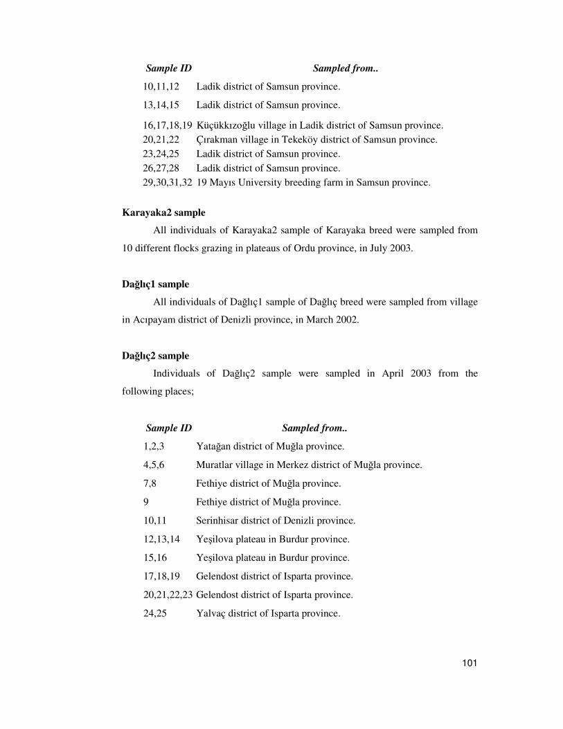
101
Sample ID Sampled from..
10,11,12 Ladik district of Samsun province.
13,14,15 Ladik district of Samsun province.
16,17,18,19 Küçükkızo�lu village in Ladik district of Samsun province. 20,21,22 Çırakman village in Tekeköy district of Samsun province. 23,24,25 Ladik district of Samsun province. 26,27,28 Ladik district of Samsun province. 29,30,31,32 19 Mayıs University breeding farm in Samsun province.
Karayaka2 sample
All individuals of Karayaka2 sample of Karayaka breed were sampled from
10 different flocks grazing in plateaus of Ordu province, in July 2003.
Da�lıç1 sample
All individuals of Da�lıç1 sample of Da�lıç breed were sampled from village
in Acıpayam district of Denizli province, in March 2002.
Da�lıç2 sample
Individuals of Da�lıç2 sample were sampled in April 2003 from the
following places;
Sample ID Sampled from..
1,2,3 Yata�an district of Mu�la province.
4,5,6 Muratlar village in Merkez district of Mu�la province.
7,8 Fethiye district of Mu�la province.
9 Fethiye district of Mu�la province.
10,11 Serinhisar district of Denizli province.
12,13,14 Ye�ilova plateau in Burdur province.
15,16 Ye�ilova plateau in Burdur province.
17,18,19 Gelendost district of Isparta province.
20,21,22,23 Gelendost district of Isparta province.
24,25 Yalvaç district of Isparta province.

102
26,27,28 E�irdir district of Isparta province.
Sample ID Sampled from..
29,36,37 Konarı village in ��çehisar district of Afyon province.
30,31,32,33 Konarı village in ��çehisar district of Afyon province.
34,35 Seydiler village in ��çehisar district of Afyon province.
38,39 Seydiler village in ��çehisar district of Afyon province.
Norduz sample
Individual samples of Norduz breed were collected from the villages of
Merkez, Muradiye and Gürpınar districts of Van province, in June 2003.
Hamdani sample
Individual samples of Hamdani breed were collected from the villages of
Merkez, Muradiye and Gürpınar districts of Van province, in June 2003. We have
been informed that the individuals of this breed were brought to Van from Iraq.
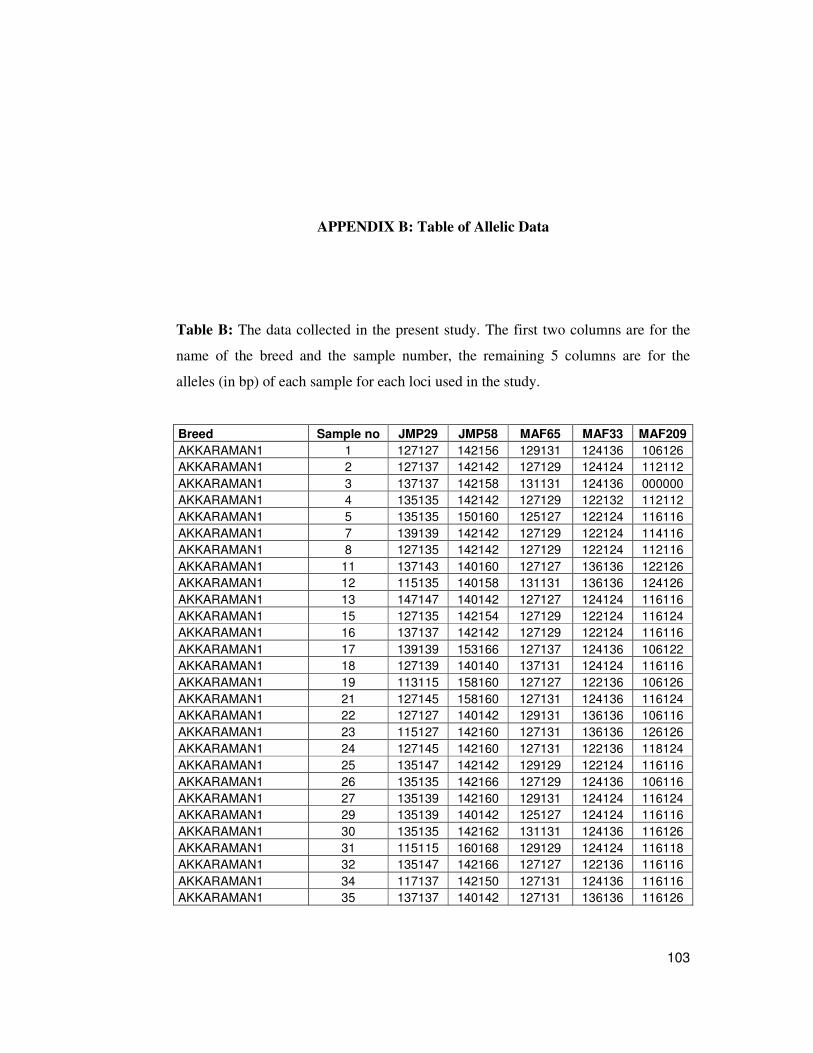
103
APPENDIX B: Table of Allelic Data
Table B: The data collected in the present study. The first two columns are for the
name of the breed and the sample number, the remaining 5 columns are for the
alleles (in bp) of each sample for each loci used in the study.
Breed Sample no JMP29 JMP58 MAF65 MAF33 MAF209 AKKARAMAN1 1 127127 142156 129131 124136 106126 AKKARAMAN1 2 127137 142142 127129 124124 112112 AKKARAMAN1 3 137137 142158 131131 124136 000000 AKKARAMAN1 4 135135 142142 127129 122132 112112 AKKARAMAN1 5 135135 150160 125127 122124 116116 AKKARAMAN1 7 139139 142142 127129 122124 114116 AKKARAMAN1 8 127135 142142 127129 122124 112116 AKKARAMAN1 11 137143 140160 127127 136136 122126 AKKARAMAN1 12 115135 140158 131131 136136 124126 AKKARAMAN1 13 147147 140142 127127 124124 116116 AKKARAMAN1 15 127135 142154 127129 122124 116124 AKKARAMAN1 16 137137 142142 127129 122124 116116 AKKARAMAN1 17 139139 153166 127137 124136 106122 AKKARAMAN1 18 127139 140140 137131 124124 116116 AKKARAMAN1 19 113115 158160 127127 122136 106126 AKKARAMAN1 21 127145 158160 127131 124136 116124 AKKARAMAN1 22 127127 140142 129131 136136 106116 AKKARAMAN1 23 115127 142160 127131 136136 126126 AKKARAMAN1 24 127145 142160 127131 122136 118124 AKKARAMAN1 25 135147 142142 129129 122124 116116 AKKARAMAN1 26 135135 142166 127129 124136 106116 AKKARAMAN1 27 135139 142160 129131 124124 116124 AKKARAMAN1 29 135139 140142 125127 124124 116116 AKKARAMAN1 30 135135 142162 131131 124136 116126 AKKARAMAN1 31 115115 160168 129129 124124 116118 AKKARAMAN1 32 135147 142166 127127 122136 116116 AKKARAMAN1 34 117137 142150 127131 124136 116116 AKKARAMAN1 35 137137 140142 127131 136136 116126

104
Table B cont'd… Breed Sample no JMP29 JMP58 MAF65 MAF33 MAF209 �VES� 1 139147 142142 129129 124128 116116 �VES� 2 137137 142150 129129 136138 126126 �VES� 4 127135 142158 129129 136136 106116 �VES� 5 115115 140150 127131 122136 116126 �VES� 6 135135 154162 129131 136136 116126 �VES� 7 133147 166166 127131 124132 106116 �VES� 9 135137 142166 127131 124136 114116 �VES� 10 000000 142148 127127 000000 102104 �VES� 11 137137 142154 127129 122124 106116 �VES� 12 137147 142162 127131 124132 124128 �VES� 13 135137 142162 129131 124136 116116 �VES� 14 127137 142158 129129 124136 126126 �VES� 17 135139 150158 127131 124136 116116 �VES� 18 127145 160166 129129 122124 116126 �VES� 19 139147 142158 127129 124124 106126 �VES� 20 125137 142162 129129 122136 126128 �VES� 21 127137 154154 129131 124124 114126 �VES� 22 135147 142158 129131 124124 114116 �VES� 24 137137 154162 129129 124124 106114 �VES� 26 127137 142162 129131 124124 114116 �VES� 28 127135 142162 127131 124132 112122 �VES� 29 137147 142142 129137 124140 116124 �VES� 30 137137 158158 129131 124136 106114 �VES� 32 135137 142156 129131 128128 116126 �VES� 34 135135 142160 133137 122138 116124 �VES� 35 135135 142142 121129 122124 000000 KIVIRCIK 1 132132 142156 127129 124136 000000 KIVIRCIK 2 127137 158164 127129 136136 110120 KIVIRCIK 3 135139 142158 127133 136136 112120 KIVIRCIK 4 127139 152160 129137 124146 110116 KIVIRCIK 5 137137 160160 123127 124126 110112 KIVIRCIK 8 135135 164164 129133 134138 112112 KIVIRCIK 9 135159 138168 127129 124124 112112 KIVIRCIK 11 127137 138138 133137 134136 112120 KIVIRCIK 12 127137 138158 131133 000000 112118 KIVIRCIK 16 135135 138158 129133 122136 110110 KIVIRCIK 18 127135 138138 123129 124124 118120 KIVIRCIK 20 137137 142160 127131 136136 110122 KIVIRCIK 21 125137 138138 129137 122126 112122 KIVIRCIK 22 127135 138138 127129 130136 112122 KIVIRCIK 23 131135 138138 127127 124136 112122 KIVIRCIK 24 131137 156166 129133 124138 110110 KIVIRCIK 25 115137 158160 127131 124136 110110 KIVIRCIK 27 000000 144156 131133 124136 114116 KIVIRCIK 29 127135 158158 129129 124134 112122 KIVIRCIK 30 127137 138138 129131 126146 110112 KIVIRCIK 33 135145 138138 127129 124136 112118

105
Table B cont'd… Breed Sample no JMP29 JMP58 MAF65 MAF33 MAF209 KIVIRCIK 34 127135 138138 129129 124136 112112 KIVIRCIK 35 127137 138138 129129 124138 110112 TÜRKGELD� 1 137147 000000 000000 124136 114116 TÜRKGELD� 3 127127 142142 127137 136138 118130 TÜRKGELD� 5 137147 142142 000000 124136 114126 TÜRKGELD� 6 137137 144144 127133 124136 116128 TÜRKGELD� 8 137139 144144 000000 124132 000000 TÜRKGELD� 11 137137 154158 129137 134136 114130 TÜRKGELD� 12 125137 142142 127127 132136 114116 TÜRKGELD� 17 125137 142142 133137 136138 114114 TÜRKGELD� 18 137137 154158 129129 134136 116128 TÜRKGELD� 19 147157 142158 127137 124136 114116 TÜRKGELD� 20 139139 140142 127129 124134 116118 TÜRKGELD� 21 137137 142142 127139 134136 116130 TÜRKGELD� 22 125137 142142 127127 132136 114116 TÜRKGELD� 23 137157 142142 127129 124136 118130 TÜRKGELD� 25 131147 142142 127129 136136 114114 TÜRKGELD� 26 157157 142154 127137 134136 116130 TÜRKGELD� 27 137139 142142 127129 136136 114116 TÜRKGELD� 28 139139 142154 127129 132134 128130 TÜRKGELD� 29 125125 142142 127137 134136 116126 TÜRKGELD� 30 137137 142154 127127 136136 116124 TÜRKGELD� 31 147147 142142 127137 134136 114130 TÜRKGELD� 32 137147 142158 127137 134136 114126 TÜRKGELD� 33 131137 142142 127127 124136 114114 TÜRKGELD� 34 147157 142142 127129 124132 118126 KONYA MER�NOSU 1 000000 000000 127131 136136 116124 KONYA MER�NOSU 2 135137 000000 000000 124124 118126 KONYA MER�NOSU 3 127127 142166 129129 124136 106118 KONYA MER�NOSU 4 143143 142160 129129 124134 106118 KONYA MER�NOSU 5 115115 142142 129129 122136 118126 KONYA MER�NOSU 6 135135 154158 127129 122136 116126 KONYA MER�NOSU 7 127127 000000 000000 136136 116124 KONYA MER�NOSU 8 127127 140142 000000 136136 106116 KONYA MER�NOSU 9 127139 142160 125129 122136 118126 KONYA MER�NOSU 10 115115 160168 000000 124136 116126 KONYA MER�NOSU 11 115135 150162 125129 124136 106126 KONYA MER�NOSU 12 135137 144160 125129 124136 106106 KONYA MER�NOSU 13 127137 160168 127127 136136 118128 KONYA MER�NOSU 14 115127 144144 129129 124136 118126 KONYA MER�NOSU 15 115115 142158 129129 136136 120128 KONYA MER�NOSU 17 137137 142144 129129 122136 126126 KONYA MER�NOSU 18 127143 160162 131131 124136 106124 KONYA MER�NOSU 19 139145 142160 127129 124136 116118 KONYA MER�NOSU 21 127127 142144 125129 136136 118126 KONYA MER�NOSU 24 000000 150160 125125 136136 118126 KONYA MER�NOSU 25 137143 144158 000000 124136 118120

106
Table B cont'd… Breed Sample no JMP29 JMP58 MAF65 MAF33 MAF209 KONYA MER�NOSU 26 115127 000000 125125 136136 000000 KONYA MER�NOSU 27 115127 140140 125129 124136 116126 KONYA MER�NOSU 28 115115 140168 125129 136136 106124 KONYA MER�NOSU 30 125137 160168 125129 122124 120128 KONYA MER�NOSU 31 115127 144160 125129 136136 128128 KONYA MER�NOSU 32 127143 144170 127129 122136 126128 KONYA MER�NOSU 33 115127 158160 127127 122136 120120 KONYA MER�NOSU 35 137143 142160 125129 122136 106118 MORKARAMAN 1 137139 150160 129129 122122 000000 MORKARAMAN 3 129137 144154 127129 122136 000000 MORKARAMAN 4 137145 144144 127137 124128 116116 MORKARAMAN 5 127137 144160 127137 122124 116126 MORKARAMAN 6 135139 144144 127127 136140 116122 MORKARAMAN 7 127137 144144 129137 126128 120124 MORKARAMAN 8 139139 144168 121129 124124 116128 MORKARAMAN 9 135151 144154 127129 124136 124132 MORKARAMAN 10 137139 150162 125129 124136 126130 MORKARAMAN 11 137139 144144 127129 122124 126126 MORKARAMAN 12 127139 144168 127135 124136 126126 MORKARAMAN 13 127137 142162 000000 136136 118126 MORKARAMAN 14 129137 144150 121129 124124 120124 MORKARAMAN 15 117139 144144 000000 124136 118118 MORKARAMAN 16 137139 150154 131135 122132 118118 MORKARAMAN 17 137139 160168 000000 136136 116116 MORKARAMAN 18 127139 144162 129131 124132 116116 MORKARAMAN 19 137141 144162 129135 122122 118118 MORKARAMAN 20 127145 144144 127129 124138 116116 MORKARAMAN 21 137137 144162 129131 122124 118124 MORKARAMAN 22 137137 144150 123131 136136 118118 MORKARAMAN 23 127129 164168 131131 124136 118124 MORKARAMAN 24 129139 144144 129129 124132 116130 MORKARAMAN 25 139147 144144 127131 124124 122126 MORKARAMAN 26 147151 144158 000000 134136 118118 MORKARAMAN 27 137141 144162 000000 000000 118118 MORKARAMAN 28 137141 144168 000000 136136 118118 MORKARAMAN 29 129129 144150 129129 136136 116132 MORKARAMAN 30 137139 144144 129131 124124 116136 MORKARAMAN 31 145149 144144 000000 124138 116128 MORKARAMAN 32 137147 144158 129137 124140 116116 MORKARAMAN 33 143149 162164 127131 122124 118128 MORKARAMAN 35 129129 144144 000000 124136 116116 MORKARAMAN 36 127129 144164 127133 122136 116116 MORKARAMAN Mork 129137 144150 129131 122122 116116 HEM��N 1 129129 144164 129131 122136 118128 HEM��N 2 137147 144150 121129 132138 116118 HEM��N 3 137139 000000 129131 000000 118126 HEM��N 4 129137 144144 131131 136136 122124
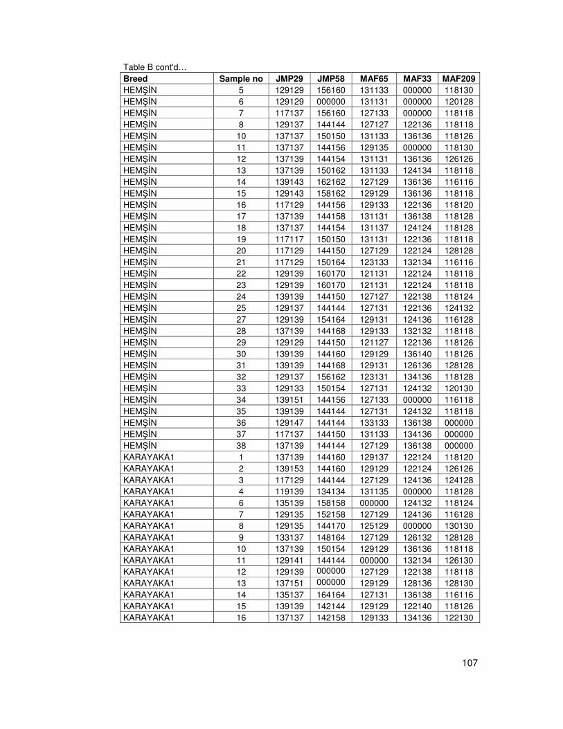
107
Table B cont'd… Breed Sample no JMP29 JMP58 MAF65 MAF33 MAF209 HEM��N 5 129129 156160 131133 000000 118130 HEM��N 6 129129 000000 131131 000000 120128 HEM��N 7 117137 156160 127133 000000 118118 HEM��N 8 129137 144144 127127 122136 118118 HEM��N 10 137137 150150 131133 136136 118126 HEM��N 11 137137 144156 129135 000000 118130 HEM��N 12 137139 144154 131131 136136 126126 HEM��N 13 137139 150162 131133 124134 118118 HEM��N 14 139143 162162 127129 136136 116116 HEM��N 15 129143 158162 129129 136136 118118 HEM��N 16 117129 144156 129133 122136 118120 HEM��N 17 137139 144158 131131 136138 118128 HEM��N 18 137137 144154 131137 124124 118128 HEM��N 19 117117 150150 131131 122136 118118 HEM��N 20 117129 144150 127129 122124 128128 HEM��N 21 117129 150164 123133 132134 116116 HEM��N 22 129139 160170 121131 122124 118118 HEM��N 23 129139 160170 121131 122124 118118 HEM��N 24 139139 144150 127127 122138 118124 HEM��N 25 129137 144144 127131 122136 124132 HEM��N 27 129139 154164 129131 124136 116128 HEM��N 28 137139 144168 129133 132132 118118 HEM��N 29 129129 144150 121127 122136 118126 HEM��N 30 139139 144160 129129 136140 118126 HEM��N 31 139139 144168 129131 126136 128128 HEM��N 32 129137 156162 123131 134136 118128 HEM��N 33 129133 150154 127131 124132 120130 HEM��N 34 139151 144156 127133 000000 116118 HEM��N 35 139139 144144 127131 124132 118118 HEM��N 36 129147 144144 133133 136138 000000 HEM��N 37 117137 144150 131133 134136 000000 HEM��N 38 137139 144144 127129 136138 000000 KARAYAKA1 1 137139 144160 129137 122124 118120 KARAYAKA1 2 139153 144160 129129 122124 126126 KARAYAKA1 3 117129 144144 127129 124136 124128 KARAYAKA1 4 119139 134134 131135 000000 118128 KARAYAKA1 6 135139 158158 000000 124132 118124 KARAYAKA1 7 129135 152158 127129 124136 116128 KARAYAKA1 8 129135 144170 125129 000000 130130 KARAYAKA1 9 133137 148164 127129 126132 128128 KARAYAKA1 10 137139 150154 129129 136136 118118 KARAYAKA1 11 129141 144144 000000 132134 126130 KARAYAKA1 12 129139 000000 127129 122138 118118 KARAYAKA1 13 137151 000000 129129 128136 128130 KARAYAKA1 14 135137 164164 127131 136138 116116 KARAYAKA1 15 139139 142144 129129 122140 118126 KARAYAKA1 16 137137 142158 129133 134136 122130

108
Table B cont'd… Breed Sample no JMP29 JMP58 MAF65 MAF33 MAF209 KARAYAKA1 17 129137 144144 131131 124136 116128 KARAYAKA1 18 129139 144160 129131 124136 126128 KARAYAKA1 19 129139 156160 129133 122124 118126 KARAYAKA1 20 129135 144156 129129 122124 118124 KARAYAKA1 21 139139 144144 127131 122136 126130 KARAYAKA1 22 129131 144144 000000 136136 118120 KARAYAKA1 23 137153 144160 000000 124136 116118 KARAYAKA1 24 137137 144144 127129 122124 118124 KARAYAKA1 25 137153 144144 127129 124136 118128 KARAYAKA1 26 137139 160162 129129 136138 126126 KARAYAKA1 27 131147 144144 123125 138146 118128 KARAYAKA1 29 137139 000000 127131 134136 000000 KARAYAKA1 30 129137 144168 127131 136136 118124 KARAYAKA1 31 137137 144168 127129 122136 116128 KARAYAKA1 32 000000 000000 127135 124136 128130 DA�LIÇ1 1 137137 144162 000000 132136 118120 DA�LIÇ1 2 000000 160160 127129 122136 118118 DA�LIÇ1 3 139141 144150 129129 130140 000000 DA�LIÇ1 4 000000 144160 000000 122136 118128 DA�LIÇ1 5 000000 152160 121126 136140 118118 DA�LIÇ1 6 137137 148158 129131 122124 116126 DA�LIÇ1 7 137141 158160 129131 122136 118128 DA�LIÇ1 8 129139 162164 129129 124136 118118 DA�LIÇ1 9 135137 162168 129129 124136 118128 DA�LIÇ1 10 139139 144168 127129 122124 118128 DA�LIÇ1 11 129149 144144 131133 122124 118126 DA�LIÇ1 12 139149 164168 000000 122124 118128 DA�LIÇ1 14 137141 150162 000000 136136 118118 DA�LIÇ1 15 137149 144168 129129 136136 116130 DA�LIÇ1 16 000000 142144 123127 124136 126126 DA�LIÇ1 17 137147 142144 131131 124136 118128 DA�LIÇ1 18 129129 144144 123129 124136 116130 DA�LIÇ1 19 131139 144150 121131 124136 118130 DA�LIÇ1 20 129143 142156 127129 122132 118126 DA�LIÇ1 21 137139 144144 123127 124136 124130 DA�LIÇ1 22 139143 164164 129131 122124 118126 DA�LIÇ1 23 137139 142160 123137 122136 116130 DA�LIÇ1 25 131139 144144 121129 122136 124124 DA�LIÇ1 26 137137 144150 129129 124136 118118 DA�LIÇ1 27 131149 144150 129133 122136 118130 DA�LIÇ1 28 131149 144164 127131 122136 118130 DA�LIÇ1 29 135137 162162 129137 122136 118118 DA�LIÇ1 30 137139 144150 129129 124130 000000 DA�LIÇ1 31 129147 142156 129129 122124 128122 DA�LIÇ1 32 117147 144164 129131 136136 118118 DA�LIÇ1 33 137139 144160 123127 122136 118128 DA�LIÇ1 34 135137 144144 127129 136136 118128

109
Table B cont'd… Breed Sample no JMP29 JMP58 MAF65 MAF33 MAF209 DA�LIÇ1 35 135139 144144 127129 136136 118118 AKKARAMAN2 1 129137 000000 000000 136140 118118 AKKARAMAN2 2 137147 150160 121131 122132 118118 AKKARAMAN2 3 143149 144154 127131 122136 118118 AKKARAMAN2 4 129129 142152 000000 122132 114118 AKKARAMAN2 5 127129 144150 000000 000000 118118 AKKARAMAN2 6 137139 144154 129131 132136 118118 AKKARAMAN2 7 139147 144162 129131 000000 118118 AKKARAMAN2 8 137139 144158 000000 000000 118128 AKKARAMAN2 9 137143 144144 129137 000000 118118 AKKARAMAN2 10 137139 144164 129129 000000 116116 AKKARAMAN2 11 137137 144158 127133 000000 000000 AKKARAMAN2 12 127127 144154 129129 000000 118118 AKKARAMAN2 13 127139 144144 000000 000000 114118 AKKARAMAN2 14 141145 144162 121126 000000 116116 AKKARAMAN2 15 137139 144150 121131 124124 116118 DA�LIÇ2 7002 137141 144168 127129 130134 114124 DA�LIÇ2 7004 137137 158160 127131 132136 118128 DA�LIÇ2 7005 137141 144162 127129 122124 106124 DA�LIÇ2 7006 129129 144164 127131 124132 118126 DA�LIÇ2 7008 137147 142144 131137 124136 118128 DA�LIÇ2 7009 137141 160162 129137 136136 118118 DA�LIÇ2 7010 141147 144164 129129 124136 118118 DA�LIÇ2 7011 139147 164168 127131 122124 119128 DA�LIÇ2 7012 129147 144144 129131 122124 118126 DA�LIÇ2 7013 139139 144168 127127 122124 118128 DA�LIÇ2 7014 135137 162168 129137 124132 118128 DA�LIÇ2 7017 129139 162164 127131 124136 118118 DA�LIÇ2 7018 131149 144150 123137 122136 118130 DA�LIÇ2 7019 131139 144144 122127 122136 124124 DA�LIÇ2 7021 131137 150150 129133 122124 120130 DA�LIÇ2 7022 137139 142160 127129 122136 116130 DA�LIÇ2 7023 139143 164164 121131 122124 118126 DA�LIÇ2 7024 137139 142144 123129 124136 124130 DA�LIÇ2 7025 131139 144150 123127 136136 118130 DA�LIÇ2 7027 129139 144144 129129 124136 116130 DA�LIÇ2 7028 135139 144144 129131 136136 118118 DA�LIÇ2 7029 137137 144144 131131 136136 118128 DA�LIÇ2 7030 137139 144160 129129 122136 118128 DA�LIÇ2 7031 117147 144164 129137 136136 118118 DA�LIÇ2 7032 129147 142156 127131 122124 128128 DA�LIÇ2 7033 147147 144150 131131 124136 118118 DA�LIÇ2 7034 135137 162162 129129 122136 118118 DA�LIÇ2 7035 137143 150154 129139 126136 118126 DA�LIÇ2 7036 135139 144170 127137 124124 118128 DA�LIÇ2 7037 127131 144160 127131 124136 118126 DA�LIÇ2 7038 139157 154158 129129 136136 118118

110
Table B cont'd… Breed Sample no JMP29 JMP58 MAF65 MAF33 MAF209 DA�LIÇ2 7039 129139 150170 125133 136138 118118 KARAYAKA2 6033 117141 158160 129129 124124 126126 KARAYAKA2 6034 139141 144154 129137 124136 118126 KARAYAKA2 6035 117129 146166 133141 124124 118128 KARAYAKA2 6036 139147 144144 127129 132136 118128 KARAYAKA2 6037 137139 156160 129129 124124 124128 KARAYAKA2 6038 131139 150150 127135 124124 118124 KARAYAKA2 6039 129141 156160 129129 136138 126128 KARAYAKA2 6040 129139 160160 131137 136138 118118 KARAYAKA2 6041 129137 162168 127129 136138 118128 KARAYAKA2 6042 137143 160160 127127 124136 118126 KARAYAKA2 6043 137139 148168 129129 136136 116128 KARAYAKA2 6044 139139 160168 127129 124136 118118 KARAYAKA2 6045 131139 144160 122133 124124 118130 KARAYAKA2 6046 139139 152166 129129 122136 118118 KARAYAKA2 6047 117131 150162 127127 124124 118118 KARAYAKA2 6048 129129 144160 129131 124124 118128 KARAYAKA2 6049 129137 150160 129133 124138 116128 KARAYAKA2 6050 137139 144170 129137 124124 126130 KARAYAKA2 6051 137139 160168 127129 122124 116116 KARAYAKA2 6052 117137 144144 127131 124132 118128 KARAYAKA2 6053 139143 144168 129131 124136 118118 KARAYAKA2 6054 137137 142166 131133 136136 126130 KARAYAKA2 6055 131151 148150 131131 134140 118130 KARAYAKA2 6056 129137 150150 133137 122124 124128 KARAYAKA2 6057 129139 156160 129131 124138 118130 KARAYAKA2 6058 137139 142160 129131 124136 118128 KARAYAKA2 6059 135139 144168 133135 122124 116128 KARAYAKA2 6060 131157 144160 129135 124138 118118 KARAYAKA2 6061 139147 144144 127133 132136 116128 AKKARAMAN3 16 139139 144160 131131 124136 118126 AKKARAMAN3 19 127129 150164 127129 124124 118118 AKKARAMAN3 20 135149 144150 129131 122122 118118 AKKARAMAN3 21 129147 144168 129131 122136 118128 AKKARAMAN3 22 129137 144154 129131 124140 118118 AKKARAMAN3 23 135137 144160 127131 122140 118118 AKKARAMAN3 24 117139 144164 129129 122124 116128 AKKARAMAN3 25 137151 144162 125127 124136 118130 AKKARAMAN3 27 129137 142144 129137 132136 118118 AKKARAMAN3 28 129137 142144 127131 136136 118128 AKKARAMAN3 29 141149 144144 123129 124124 118128 AKKARAMAN3 31 129129 144164 129131 124136 118118 AKKARAMAN3 32 137141 158160 127131 124124 118118 AKKARAMAN3 33 129129 144158 129131 134136 118118 NORDUZ 13001 129139 144162 131131 124136 106118 NORDUZ 13003 127137 142168 127129 122132 128128 NORDUZ 13005 129147 144144 127129 132140 118128

111
Table B cont'd… Breed Sample no JMP29 JMP58 MAF65 MAF33 MAF209 NORDUZ 13006 129129 144150 127127 122132 120128 NORDUZ 13007 137151 144162 129129 124136 120128 NORDUZ 13008 137151 142144 129129 124136 118120 NORDUZ 13009 137141 160162 127129 124124 116116 NORDUZ 13010 139139 000000 127129 122122 120128 NORDUZ 13011 137147 150154 127129 124132 118128 NORDUZ 13012 139147 144162 129131 124136 116118 NORDUZ 13013 139143 144144 129131 124136 106118 NORDUZ 13014 129129 142144 127129 124124 118118 NORDUZ 13015 129129 144156 129129 124138 116118 NORDUZ 13016 117137 144162 127135 124136 116118 NORDUZ 13017 139139 150152 129129 122124 128130 NORDUZ 13018 129137 144144 119135 124136 118128 NORDUZ 13019 135139 144144 127129 124136 128130 NORDUZ 13020 127137 144150 119133 124124 128132 NORDUZ 13021 131141 144154 123131 124134 118128 NORDUZ 13023 137151 144154 129129 122136 118128 NORDUZ 13024 137141 160168 127129 128136 118118 NORDUZ 13025 129141 144160 131135 132136 118118 NORDUZ 13026 139145 150162 129129 136136 106118 NORDUZ 13027 135141 144150 129129 122132 128130 NORDUZ 13029 129137 144144 129129 124136 118130 NORDUZ 13028 129137 144144 131141 136136 118128 HAMDANI 14001 137139 144150 125129 124136 118128 HAMDANI 14002 137139 144154 121125 136140 118120 HAMDANI 14004 129129 144144 127131 124136 118128 HAMDANI 14005 137147 144150 129129 122136 116118 HAMDANI 14006 139151 144154 131131 124124 000000 HAMDANI 14007 137139 144168 129131 132136 128130 HAMDANI 14008 129139 164168 129129 122136 118118 HAMDANI 14009 139139 144144 000000 124136 116118 HAMDANI 14010 137139 144154 127133 124136 116128 HAMDANI 14011 139141 144144 129129 122136 000000 HAMDANI 14012 137139 144150 125129 122124 124128 HAMDANI 14013 137139 154164 127129 136136 000000 HAMDANI 14014 137139 144144 129129 124132 000000 HAMDANI 14015 139147 150154 129129 124136 120128 HAMDANI 14016 137137 144144 127129 122136 118118 HAMDANI 14017 137137 144144 131141 136136 126128 HAMDANI 14018 127129 144150 129131 136136 118118 HAMDANI 14019 137137 158168 131131 122124 118128 HAMDANI 14020 127137 150168 129131 122136 106128 HAMDANI 14021 139139 144144 127129 124124 118128 HAMDANI 14022 129139 144150 129129 124132 128132 HAMDANI 14023 129137 144150 129133 124124 118118 KANGAL 15001 135147 144160 129131 124124 118120 KANGAL 15002 141147 144162 129129 122124 116120

112
Table B cont'd… Breed Sample no JMP29 JMP58 MAF65 MAF33 MAF209 KANGAL 15003 125145 144160 127129 136136 118118 KANGAL 15004 137141 144150 127129 124136 116120 KANGAL 15005 129137 144168 127131 124136 116128 KANGAL 15006 127129 160168 131137 124140 118118 KANGAL 15007 139147 144144 129131 136136 126128 KANGAL 15008 129137 144164 127133 124124 128128 KANGAL 15009 129129 160160 127127 124124 118118 KANGAL 15010 129137 144168 127133 000000 000000 KANGAL 15011 139139 144168 129131 122124 114118 KANGAL 15012 129129 144160 123131 124124 116118 KANGAL 15013 137139 144144 129131 122124 118118 KANGAL 15014 137143 154164 127129 124140 118128 KANGAL 15015 129147 158160 129129 124136 118118 KANGAL 15016 151151 144150 129129 124124 118128 KANGAL 15017 137137 160168 131131 124136 114118 KANGAL 15018 139151 144144 109131 132136 118126 KANGAL 15019 129139 150154 131131 122124 118130 KANGAL 15020 137139 142168 129131 124124 114118 KANGAL 15022 129147 144164 127131 124138 108118 KANGAL 15023 129137 144160 127129 122132 118128 KANGAL 15024 129137 144168 127133 122134 118118

113
APPENDIX C: Table of Allele Frequencies
A
kk1
Akk
2 Iv
e K
ıv
TG
K
M
Mor
k H
em
Kry
1 K
ry2
Da�
1 D
a�2
Nor
H
am
Kng
l M
AF3
3
(N)
28
19
28
22
24
29
34
30
26
29
32
32
26
22
22
122
0,17
9 0,
211
0,16
1 0,
046
0,00
0 0,
138
0,19
1 0,
167
0,17
3 0,
069
0,23
4 0,
188
0,13
5 0,
159
0,13
6 12
4 0,
446
0,34
2 0,
429
0,34
1 0,
188
0,22
4 0,
353
0,15
0 0,
231
0,48
3 0,
234
0,28
1 0,
365
0,34
1 0,
523
126
0,00
0 0,
000
0,00
0 0,
068
0,00
0 0,
000
0,01
5 0,
017
0,01
9 0,
000
0,00
0 0,
016
0,00
0 0,
000
0,00
0 12
8 0,
000
0,00
0 0,
054
0,00
0 0,
000
0,00
0 0,
029
0,00
0 0,
019
0,00
0 0,
000
0,00
0 0,
019
0,00
0 0,
000
130
0,00
0 0,
000
0,00
0 0,
023
0,00
0 0,
000
0,00
0 0,
000
0,00
0 0,
000
0,03
1 0,
016
0,00
0 0,
000
0,00
0 13
2 0,
018
0,10
5 0,
054
0,00
0 0,
104
0,00
0 0,
044
0,10
0 0,
058
0,05
2 0,
031
0,04
7 0,
115
0,06
8 0,
046
134
0,00
0 0,
026
0,00
0 0,
068
0,18
8 0,
017
0,01
5 0,
067
0,03
9 0,
017
0,00
0 0,
016
0,01
9 0,
000
0,02
3 13
6 0,
357
0,26
3 0,
250
0,34
1 0,
479
0,62
1 0,
294
0,40
0 0,
346
0,25
9 0,
438
0,42
2 0,
308
0,40
9 0,
205
138
0,00
0 0,
000
0,03
6 0,
068
0,04
2 0,
000
0,02
9 0,
083
0,07
7 0,
103
0,00
0 0,
016
0,01
9 0,
000
0,02
3 14
0 0,
000
0,05
3 0,
018
0,00
0 0,
000
0,00
0 0,
029
0,01
7 0,
019
0,01
7 0,
031
0,00
0 0,
019
0,02
3 0,
046
146
0,00
0 0,
000
0,00
0 0,
046
0,00
0 0,
000
0,00
0 0,
000
0,01
9 0,
000
0,00
0 0,
000
0,00
0 0,
000
0,00
0 M
AF6
5
A
kk1
Akk
2 Iv
e K
ıv
TG
K
M
Mor
k H
em
Kry
1 K
ry2
Da�
1 D
a�2
Nor
H
am
Kng
l (N
) 28
23
35
23
21
24
27
34
24
29
29
32
26
21
22
10
9 0,
000
0,00
0 0,
000
0,00
0 0,
000
0,00
0 0,
000
0,00
0 0,
000
0,00
0 0,
000
0,00
0 0,
000
0,00
0 0,
023
119
0,00
0 0,
000
0,00
0 0,
000
0,00
0 0,
000
0,00
0 0,
000
0,00
0 0,
000
0,00
0 0,
000
0,03
9 0,
000
0,00
0 12
1 0,
000
0,06
5 0,
014
0,00
0 0,
000
0,00
0 0,
037
0,05
9 0,
000
0,00
0 0,
052
0,01
6 0,
000
0,02
4 0,
000
123
0,00
0 0,
022
0,00
0 0,
044
0,00
0 0,
000
0,01
9 0,
029
0,02
1 0,
017
0,08
6 0,
063
0,01
9 0,
000
0,02
3
Tab
le C
: The
alle
le fr
eque
ncy
dist
ribu
tion
of e
ach
locu
s ac
ross
the
sam
ples
. The
nam
e of
the
locu
s an
d
the
alle
les
are
give
n in
the
firs
t col
umn,
N is
the
sam
ple
size
for t
he c
orrs
pond
ing
locu
s.

114
Tabl
e C
con
t'd…
M
AF6
5
A
kk1
Akk
2 Iv
e K
ıv
TG
K
M
Mor
k H
em
Kry
1 K
ry2
Da�
1 D
a�2
Nor
H
am
Kng
l (N
) 28
23
35
23
21
24
27
34
24
29
29
32
26
21
22
12
5 0,
036
0,02
2 0,
014
0,00
0 0,
000
0,27
1 0,
019
0,00
0 0,
042
0,00
0 0,
000
0,01
6 0,
000
0,07
1 0,
000
127
0,41
1 0,
152
0,18
6 0,
239
0,52
4 0,
167
0,22
2 0,
191
0,20
8 0,
190
0,17
2 0,
219
0,21
2 0,
119
0,22
7 12
9 0,
250
0,37
0 0,
457
0,39
1 0,
214
0,50
0 0,
370
0,20
6 0,
500
0,37
9 0,
466
0,32
8 0,
500
0,50
0 0,
341
131
0,26
8 0,
326
0,27
1 0,
109
0,00
0 0,
063
0,18
5 0,
324
0,14
6 0,
155
0,15
5 0,
219
0,13
5 0,
214
0,31
8 13
3 0,
000
0,00
0 0,
014
0,15
2 0,
048
0,00
0 0,
019
0,16
2 0,
042
0,12
1 0,
035
0,03
1 0,
019
0,04
8 0,
046
135
0,00
0 0,
000
0,00
0 0,
000
0,00
0 0,
000
0,05
6 0,
015
0,02
1 0,
052
0,00
0 0,
000
0,05
8 0,
000
0,00
0 13
7 0,
036
0,04
4 0,
029
0,06
5 0,
191
0,00
0 0,
074
0,01
5 0,
021
0,06
9 0,
035
0,09
4 0,
000
0,00
0 0,
023
139
0,00
0 0,
000
0,01
4 0,
000
0,02
4 0,
000
0,00
0 0,
000
0,00
0 0,
000
0,00
0 0,
016
0,00
0 0,
000
0,00
0 14
1 0,
000
0,00
0 0,
000
0,00
0 0,
000
0,00
0 0,
000
0,00
0 0,
000
0,01
7 0,
000
0,00
0 0,
019
0,02
4 0,
000
MA
F209
A
kk1
Akk
2 Iv
e K
ıv
TG
K
M
Mor
k H
em
Kry
1 K
ry2
Da�
1 D
a�2
Nor
H
am
Kng
l (N
) 27
24
34
22
23
28
33
31
28
29
30
32
26
18
22
10
6 0,
093
0,00
0 0,
088
0,00
0 0,
000
0,16
1 0,
000
0,00
0 0,
000
0,00
0 0,
000
0,01
6 0,
058
0,02
8 0,
000
108
0,00
0 0,
000
0,00
0 0,
000
0,00
0 0,
000
0,00
0 0,
000
0,00
0 0,
000
0,00
0 0,
000
0,00
0 0,
000
0,02
3 11
0 0,
000
0,00
0 0,
000
0,27
3 0,
000
0,00
0 0,
000
0,00
0 0,
000
0,00
0 0,
000
0,00
0 0,
000
0,00
0 0,
000
112
0,09
3 0,
000
0,01
5 0,
386
0,00
0 0,
000
0,00
0 0,
000
0,00
0 0,
000
0,00
0 0,
000
0,00
0 0,
000
0,00
0 11
4 0,
019
0,02
1 0,
088
0,02
3 0,
326
0,00
0 0,
000
0,00
0 0,
000
0,00
0 0,
000
0,01
6 0,
000
0,00
0 0,
068
MA
F209
A
kk1
Akk
2 Iv
e K
ıv
TG
K
M
Mor
k H
em
Kry
1 K
ry2
Da�
1 D
a�2
Nor
H
am
Kng
l (N
) 27
24
34
22
23
28
33
31
28
29
30
32
26
18
22
11
6 0,
482
0,12
5 0,
265
0,04
6 0,
261
0,12
5 0,
349
0,11
3 0,
107
0,10
3 0,
067
0,03
1 0,
096
0,08
3 0,
091

115
Tab
le C
con
t'd
MA
F209
A
kk1
Akk
2 Iv
e K
ıv
TG
K
M
Mor
k H
em
Kry
1 K
ry2
Da�
1 D
a�2
Nor
H
am
Kng
l (N
) 27
24
34
22
23
28
33
31
28
29
30
32
26
18
22
11
8 0,
037
0,72
9 0,
206
0,06
8 0,
087
0,21
4 0,
273
0,50
0 0,
286
0,41
4 0,
500
0,50
0 0,
385
0,41
7 0,
523
120
0,00
0 0,
000
0,00
0 0,
091
0,00
0 0,
089
0,03
0 0,
032
0,03
6 0,
000
0,01
7 0,
031
0,07
7 0,
056
0,06
8 12
2 0,
037
0,00
0 0,
015
0,11
4 0,
000
0,00
0 0,
030
0,01
6 0,
018
0,00
0 0,
017
0,00
0 0,
000
0,00
0 0,
000
124
0,09
3 0,
000
0,07
4 0,
000
0,02
2 0,
071
0,07
6 0,
048
0,08
9 0,
052
0,05
0 0,
078
0,00
0 0,
028
0,00
0 12
6 0,
148
0,02
1 0,
162
0,00
0 0,
087
0,23
2 0,
121
0,08
1 0,
161
0,12
1 0,
100
0,07
8 0,
000
0,02
8 0,
046
128
0,00
0 0,
083
0,08
8 0,
000
0,06
5 0,
107
0,04
6 0,
145
0,19
6 0,
224
0,13
3 0,
156
0,28
9 0,
306
0,15
9 13
0 0,
000
0,02
1 0,
000
0,00
0 0,
152
0,00
0 0,
030
0,04
8 0,
107
0,08
6 0,
117
0,09
4 0,
077
0,02
8 0,
023
132
0,00
0 0,
000
0,00
0 0,
000
0,00
0 0,
000
0,03
0 0,
016
0,00
0 0,
000
0,00
0 0,
000
0,01
9 0,
028
0,00
0 13
6 0,
000
0,00
0 0,
000
0,00
0 0,
000
0,00
0 0,
015
0,00
0 0,
000
0,00
0 0,
000
0,00
0 0,
000
0,00
0 0,
000
JMP2
9
A
kk1
Akk
2 Iv
e K
ıv
TG
K
M
Mor
k H
em
Kry
1 K
ry2
Da�
1 D
a�2
Nor
H
am
Kng
l (N
) 28
24
35
22
24
27
35
34
28
29
29
32
26
22
22
11
3 0,
018
0,00
0 0,
000
0,00
0 0,
000
0,00
0 0,
000
0,00
0 0,
000
0,00
0 0,
000
0,00
0 0,
000
0,00
0 0,
000
115
0,08
9 0,
000
0,02
9 0,
023
0,00
0 0,
259
0,00
0 0,
000
0,00
0 0,
000
0,00
0 0,
000
0,00
0 0,
000
0,00
0 11
7 0,
018
0,02
1 0,
000
0,00
0 0,
000
0,00
0 0,
014
0,10
3 0,
018
0,06
9 0,
017
0,01
6 0,
019
0,00
0 0,
000
119
0,00
0 0,
000
0,00
0 0,
000
0,00
0 0,
000
0,00
0 0,
000
0,01
8 0,
000
0,00
0 0,
000
0,00
0 0,
000
0,00
0 12
5 0,
000
0,00
0 0,
014
0,02
3 0,
104
0,01
9 0,
000
0,00
0 0,
000
0,00
0 0,
000
0,00
0 0,
000
0,00
0 0,
023
127
0,19
6 0,
063
0,08
6 0,
227
0,04
2 0,
315
0,11
4 0,
000
0,00
0 0,
000
0,00
0 0,
016
0,03
9 0,
046
0,02
3 12
9 0,
000
0,22
9 0,
071
0,00
0 0,
000
0,00
0 0,
143
0,27
9 0,
196
0,15
5 0,
103
0,10
9 0,
231
0,13
6 0,
273
131
0,00
0 0,
000
0,00
0 0,
091
0,04
2 0,
000
0,00
0 0,
000
0,03
6 0,
086
0,06
9 0,
078
0,01
9 0,
000
0,00
0

116
Tab
le C
con
t'd…
JM
P29
Akk
1 A
kk2
Ive
Kıv
T
G
KM
M
ork
Hem
K
ry1
Kry
2 D
a�1
Da�
2 N
or
Ham
K
ngl
(N)
28
24
35
22
24
27
35
34
28
29
29
32
26
22
22
133
0,00
0 0,
000
0,01
4 0,
000
0,00
0 0,
000
0,00
0 0,
015
0,01
8 0,
000
0,00
0 0,
000
0,00
0 0,
000
0,00
0 13
5 0,
268
0,04
2 0,
200
0,27
3 0,
000
0,09
3 0,
029
0,00
0 0,
089
0,01
7 0,
069
0,06
3 0,
039
0,00
0 0,
023
137
0,16
1 0,
229
0,28
6 0,
273
0,41
7 0,
148
0,30
0 0,
265
0,28
6 0,
207
0,29
3 0,
234
0,23
1 0,
364
0,22
7 13
9 0,
125
0,14
6 0,
143
0,04
6 0,
125
0,03
7 0,
200
0,26
5 0,
232
0,31
0 0,
224
0,23
4 0,
173
0,36
4 0,
159
141
0,00
0 0,
063
0,02
9 0,
000
0,00
0 0,
000
0,04
3 0,
000
0,01
8 0,
052
0,05
2 0,
063
0,09
6 0,
023
0,04
6 14
3 0,
018
0,04
2 0,
000
0,00
0 0,
000
0,11
1 0,
014
0,02
9 0,
000
0,03
5 0,
035
0,03
1 0,
019
0,00
0 0,
023
145
0,03
6 0,
021
0,01
4 0,
023
0,00
0 0,
019
0,04
3 0,
000
0,00
0 0,
000
0,00
0 0,
000
0,01
9 0,
000
0,02
3 14
7 0,
071
0,06
3 0,
114
0,00
0 0,
167
0,00
0 0,
043
0,02
9 0,
018
0,03
5 0,
052
0,12
5 0,
058
0,04
6 0,
114
149
0,00
0 0,
063
0,00
0 0,
000
0,00
0 0,
000
0,02
9 0,
000
0,00
0 0,
000
0,08
6 0,
016
0,00
0 0,
000
0,00
0 15
1 0,
000
0,02
1 0,
000
0,00
0 0,
000
0,00
0 0,
029
0,01
5 0,
018
0,01
7 0,
000
0,00
0 0,
058
0,02
3 0,
068
153
0,00
0 0,
000
0,00
0 0,
000
0,00
0 0,
000
0,00
0 0,
000
0,05
4 0,
000
0,00
0 0,
000
0,00
0 0,
000
0,00
0 15
7 0,
000
0,00
0 0,
000
0,00
0 0,
104
0,00
0 0,
000
0,00
0 0,
000
0,01
7 0,
000
0,01
6 0,
000
0,00
0 0,
000
159
0,00
0 0,
000
0,00
0 0,
023
0,00
0 0,
000
0,00
0 0,
000
0,00
0 0,
000
0,00
0 0,
000
0,00
0 0,
000
0,00
0 JM
P58
Akk
1 A
kk2
Ive
Kıv
T
G
KM
M
ork
Hem
K
ry1
Kry
2 D
a�1
Da�
2 N
or
Ham
K
ngl
134
0,00
0 0,
000
0,00
0 0,
000
0,00
0 0,
000
0,00
0 0,
000
0,03
9 0,
000
0,00
0 0,
000
0,00
0 0,
000
0,00
0 13
8 0,
000
0,00
0 0,
000
0,45
7 0,
000
0,00
0 0,
000
0,00
0 0,
000
0,00
0 0,
000
0,00
0 0,
000
0,00
0 0,
000
140
0,14
3 0,
000
0,01
4 0,
000
0,02
2 0,
080
0,00
0 0,
000
0,00
0 0,
000
0,00
0 0,
000
0,00
0 0,
000
0,00
0 14
2 0,
464
0,06
3 0,
286
0,06
5 0,
696
0,22
0 0,
014
0,00
0 0,
039
0,03
5 0,
078
0,06
3 0,
060
0,00
0 0,
023
144
0,00
0 0,
458
0,12
9 0,
022
0,08
7 0,
160
0,55
7 0,
397
0,48
1 0,
224
0,39
1 0,
375
0,50
0 0,
546
0,40
9 14
6 0,
000
0,00
0 0,
000
0,00
0 0,
000
0,00
0 0,
000
0,00
0 0,
000
0,01
7 0,
000
0,00
0 0,
000
0,00
0 0,
000
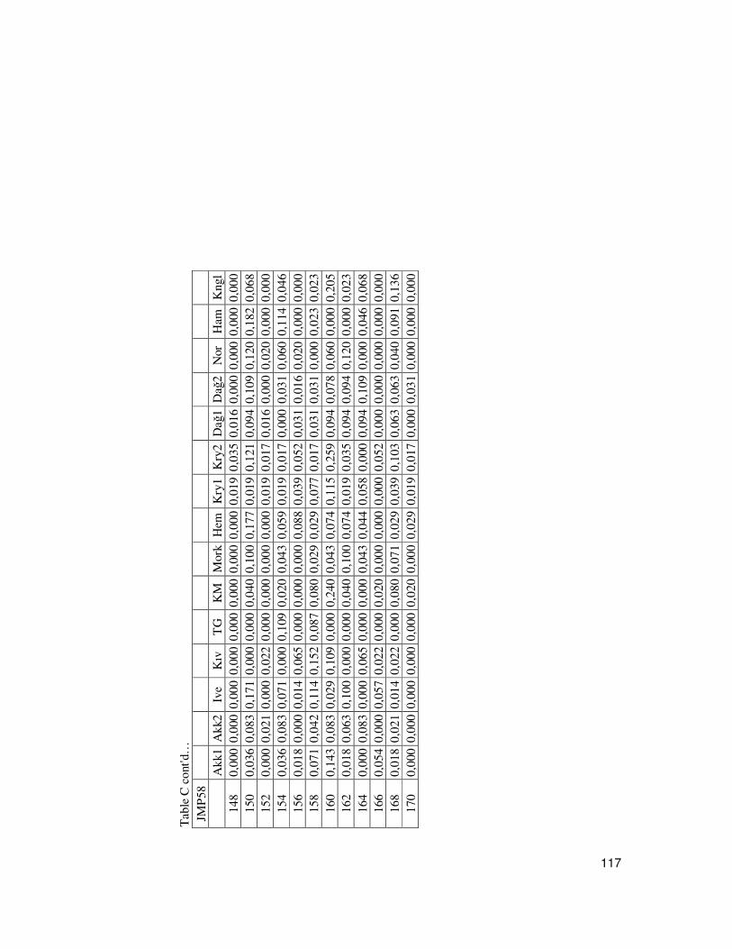
117
Tab
le C
con
t'd…
JM
P58
Akk
1 A
kk2
Ive
Kıv
T
G
KM
M
ork
Hem
K
ry1
Kry
2 D
a�1
Da�
2 N
or
Ham
K
ngl
148
0,00
0 0,
000
0,00
0 0,
000
0,00
0 0,
000
0,00
0 0,
000
0,01
9 0,
035
0,01
6 0,
000
0,00
0 0,
000
0,00
0 15
0 0,
036
0,08
3 0,
171
0,00
0 0,
000
0,04
0 0,
100
0,17
7 0,
019
0,12
1 0,
094
0,10
9 0,
120
0,18
2 0,
068
152
0,00
0 0,
021
0,00
0 0,
022
0,00
0 0,
000
0,00
0 0,
000
0,01
9 0,
017
0,01
6 0,
000
0,02
0 0,
000
0,00
0 15
4 0,
036
0,08
3 0,
071
0,00
0 0,
109
0,02
0 0,
043
0,05
9 0,
019
0,01
7 0,
000
0,03
1 0,
060
0,11
4 0,
046
156
0,01
8 0,
000
0,01
4 0,
065
0,00
0 0,
000
0,00
0 0,
088
0,03
9 0,
052
0,03
1 0,
016
0,02
0 0,
000
0,00
0 15
8 0,
071
0,04
2 0,
114
0,15
2 0,
087
0,08
0 0,
029
0,02
9 0,
077
0,01
7 0,
031
0,03
1 0,
000
0,02
3 0,
023
160
0,14
3 0,
083
0,02
9 0,
109
0,00
0 0,
240
0,04
3 0,
074
0,11
5 0,
259
0,09
4 0,
078
0,06
0 0,
000
0,20
5 16
2 0,
018
0,06
3 0,
100
0,00
0 0,
000
0,04
0 0,
100
0,07
4 0,
019
0,03
5 0,
094
0,09
4 0,
120
0,00
0 0,
023
164
0,00
0 0,
083
0,00
0 0,
065
0,00
0 0,
000
0,04
3 0,
044
0,05
8 0,
000
0,09
4 0,
109
0,00
0 0,
046
0,06
8 16
6 0,
054
0,00
0 0,
057
0,02
2 0,
000
0,02
0 0,
000
0,00
0 0,
000
0,05
2 0,
000
0,00
0 0,
000
0,00
0 0,
000
168
0,01
8 0,
021
0,01
4 0,
022
0,00
0 0,
080
0,07
1 0,
029
0,03
9 0,
103
0,06
3 0,
063
0,04
0 0,
091
0,13
6 17
0 0,
000
0,00
0 0,
000
0,00
0 0,
000
0,02
0 0,
000
0,02
9 0,
019
0,01
7 0,
000
0,03
1 0,
000
0,00
0 0,
000

118
APPENDIX D: Allele Frequency Distribution Graphs
Figure D.1. The frequency distribution of the alleles of MAF33 locus for native
breeds
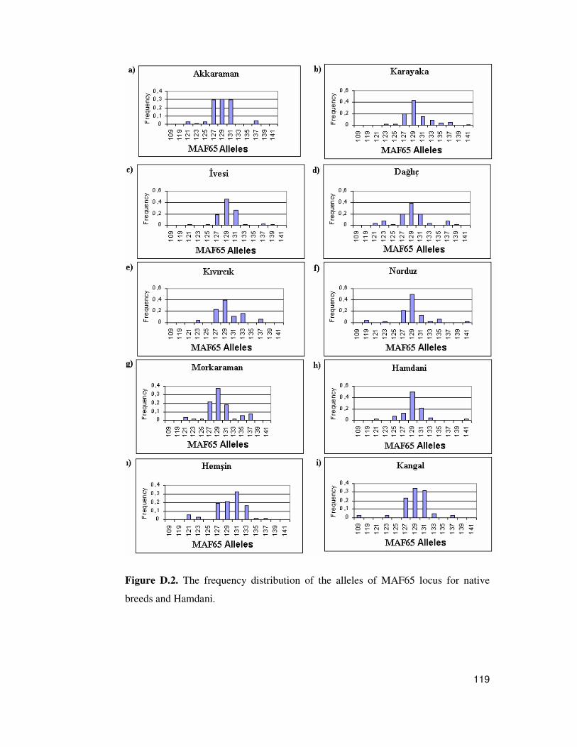
119
Figure D.2. The frequency distribution of the alleles of MAF65 locus for native
breeds and Hamdani.

120
Figure D.3. The frequency distribution of the alleles of MAF209 locus for native
breeds and Hamdani.

121
Figure D.4. The frequency distribution of the alleles of JMP29 locus for native
breeds and Hamdani.

122
Figure D.5. The frequency distribution of the alleles of JMP58 locus for native
breeds and Hamdani.

123
CURRICULUM VITAE
PERSONAL INFORMATION Surname, Name: Koban, Evren Nationality: Turkish (TC) Date and Place of Birth: 11 June 1976, �stanbul Marital Status: Single Phone: +90 312 210 5179 Fax: +90 312 210 1289 E-mail: [email protected] EDUCATION
Degree Institution Year of Graduation MS METU, Biology 2001 BS METU, Biology Education 1998 High School Ayrancı Lisesi, Ankara 1993
WORK EXPERIENCE Year Place Enrollment 2004-present METU Central Lab, Molecular Biology and
Biotechnology Research and Development Unit Research Assistant
FOREIGN LANGUAGES Advanced English PUBLICATIONS Soysal M. �., Koban E., Özkan E., Altunok V., Bulut Z., Nizamlıo�lu M. and Togan �. Evolutionary relationship among three native and two crossbreed sheep breeds of Turkey: preliminary results. Revue de Medecine Veterinaire, in press. Koban E., Altunok V., Chikhi L., Schaffer A., Pedersen N. C., Nizamlıo�lu M. and Togan �. Genetic evidence for distinctness of Kangal dogs. Submitted article.

124
PRESENTATIONS AT NATIONAL AND INTERNATIONAL CONGRESS Bulut Z., Nizamlıo�lu M., Togan I., Koban, E. (2004). Konya Bölgesi’nde bulunan bazı koyun ırklarının genetic yapılarının mikrosatellit markerlarla incelenmesi. Biyoinformatik-I Yüksek Lisans Yaz Okulu, Antalya, Turkey. Togan I., Berkman C.C., Koban E. (2004). Molecular Markers in Conservation. Workshop on Conservation of Native Genetic Resources, Tekirda�, Turkey. Koban E., Özkan E., Altunok V., Nizamlıo�lu M., Soysal �., Bruford M.W., Togan �. (2003). Genetic diversity within and among Turkish sheep breeds, their domestication histories and conservation. Population Genetics for Animal Conservation, Trento, Italy. Koban E., Altunok V., Nizamlıo�lu M. ve Togan �. (2003). Employement of some molecular techniques to answer some questions and problems related with Kangal dog. First International Kangal Dog Symposium, Sivas, Turkey, page 67. Togan, �., Soysal M.�., Altunok V., Özkan E., Koban E., (2003). Populasyon Geneti�i Çalı�malarında Kullanılan �statistiksel Yöntemlerdeki Yeniliklere Örnekler. GAP III. Tarım Kongresi (02-03 Ekim 2003). Harran Üniversitesi Ziraat Fakültesi, �anlıurfa, Turkey. Koban E., Altunok V., Soysal M.�., Ergüven A., Bruford M.W., Togan �. (2002). A preliminary study on the genetic diversity of native domestic sheep breeds in Anatolia. Phlogeography in Southern European Refugia: Evolutionary perspectives on the origins and conservation of European biodiversity, Vairão, Portugal, page 52. Koban E., Altunok V., Chikhi L., Ergüven A., Pedersen N.C., Togan �. (2002). Genetic diversity in Anatolian shepherd dogs. Phlogeography in Southern European Refugia: Evolutionary perspectives on the origins and conservation of European biodiversity, Vairão, Portugal, page 52. Özer F., Plan E., Koban E., Berkman C., Emre Y., Ergüven A., Togan �. (2002). Genetic diversity of brown trout (Salmo trutta L.) in Anatolia. Phlogeography in Southern European Refugia: Evolutionary perspectives on the origins and conservation of European biodiversity, Vairão, Portugal, page 46. Berkman C., Koban E., Togan �. (2002). Conservation of Rainbow trout (Oncorhynchus mykiss) stocks in Southern Aegean and Western Mediterranean Regions in Turkey based on molecular methods. XVI. National Biology Congress, Malatya, Turkey. Koban E., Altunok V., Chikhi L., Ergüven A. and Togan �. (2001). A genetic study on the Anatolian shepherd dog based on 100 loci. Canid Biology and Conservation Conference, Oxford, UK, page 69.

125
Koban, E., Özba� Gerçeker, F., Ergüven, A., Özgüç, M. and Togan, �., 2000. Alu insertion polymorphisms in Anatolia. XV. National Biology Congress (with international participation), Ankara, Turkey, page 33. Koban, E., Plan, E., Gezgin, F., Caner, C., Ergüven, A. and Togan, �. (2000). Genetic relation among brown trout (Salmo trutta L.) samples of Anatolia and neighboring countries. XV. National Biology Congress (with international participation), Ankara, Turkey, page 33. PROJECTS WORKED AS RESEARCHER TBAG-2127 (2001-2004): “Genetik diversity among native sheep breeds”. Directed by Prof. Dr. �nci Togan. Supported by Turkish Scientific and Technical Research Council (TUBITAK). 2000-2003: “The study on the native domestic sheep breeds in Anatolia; genetic diversity and distinctiveness”. Directed by Prof. Dr. �nci Togan and Prof. Dr. Mike Bruford. Supported by the British Council Turkey. TOGTAG/TARP-1811 (1998-2001): “Conservation of rainbow trout (Oncorhynchus mykiss) stocks in South Aegean and Western Mediterranean regions in Turkey based on molecular methods”. Directed by Prof. Dr. �nci Togan. Supported by TUBITAK. VHAG-1553 (1999-2001): “A study on the genetic structure of native and crossbred sheep breeds of Turkey based on microsatellite markers”. Directed by Prof. Dr. M. �hsan Soysal. Supported by TUBITAK. VHAG-1396 (1998-1999): “Conservation of brown trout (Salmo trutta) living in Lake Abant and Southeastern Anatolia”. Directed by Prof. Dr. �nci Togan. Supported by TUBITAK. WORKSHOPS ATTTENDED Population Genetics for Animal Conservation. 4-7 Eylül 2003, Trento, Italy.
International Workshop on Shallow Lakes and Wetlands: Ecology, Eutrophication and Restoration. 28-30 Kasım 2001, Orta Do�u Teknik Üniversitesi, Ankara, Turkey.
Population Viability Analysis (PVA) Workshop: Applications of RAMAS. 12-14 Mayıs 1999, Orta Do�u Teknik Üniversitesi, Ankara, Turkey.