genetic analysis of head morphology traits in heading

Genetic analysis of head

morphology traits in Heading

Cabbage (B. oleracea)

By: Pim van de Mortel

Master Thesis Plant Breeding (PBR-80436)

Genetic analysis of leaf and head morphology traits in heading

cabbage (B. oleracea)

By

Pim van de Mortel

930621584100

Supervisors: Guusje Bonnema & Johan Bucher

Examiners: Guusje Bonnema & Paul Arens

University: Plant Breeding Department

Wageningen University

Droevendaalsesteeg 1

6708 PB Wageningen

The Netherlands

Date: 16 December 2018

Table of Contents Abstract .................................................................................................................... 1

Acknowledgement ...................................................................................................... 2

1. Introduction ........................................................................................................... 3

1.1 Research Questions ............................................................................................ 6

2. Materials & Methods ................................................................................................ 7

2.1 Genotyping ........................................................................................................ 7

2.2 Selection of accessions ........................................................................................ 8

2.3 Field trial .......................................................................................................... 10

2.4 Phenotyping ..................................................................................................... 11

2.5 Population Structure .......................................................................................... 13

2.6 GWAS .............................................................................................................. 14

3. Results ................................................................................................................. 15

3.1 Phenotyping data .............................................................................................. 15

3.2 Population Structure .......................................................................................... 18

3.3 GWAS .............................................................................................................. 19

3.4 Physically linked SNPs and SNPs associated to several traits .................................... 25

3.5 Candidate genes ............................................................................................... 27

4. Discussion ............................................................................................................ 30

References ............................................................................................................... 36

Appendix 1. Overview of the field layout .................................................................... 42

Appendix 2. Guideline of measuring manually in ImageJ ............................................... 43

Appendix 3. Guideline for PCO in DARwin ................................................................... 44

Appendix 4. Guideline for GWAS in Tassel .................................................................. 45

Appendix 5. PCO of 180 axes for the heading cabbage subset ....................................... 46

Appendix 6. PCO of 137 axes for the 137 harvested heading cabbage subset ................... 48

Appendix 7. Manhattan plots of GWAS with 1st measurement of leafs with a PCO

of 180 axes ............................................................................................................ 49

Appendix 8. The Manhattan plots of the GWAS with the cabbage width data with

a PCO of 180 axes. ................................................................................................. 52

Appendix 9. Manhattan plots of GWAS with the 137 harvested cabbages, data

adjusted for DAS and a PCO of 137 axes. ................................................................... 53

Appendix 10. All significant SNPs found ...................................................................... 56

1

Abstract A field trial with 404 different accessions of seven different morphotypes of B. oleracea was

done in 2018. The leafs and cabbage heads of these accessions where phenotyped. For the

leafs this was leaf length, leaf width, leaf area, leaf ratio (length / width), petiole length and

petiole width. Leaf traits were measured twice, between 62 and 70 Days After Sowing (DAS)

and between 83 and 86 DAS. The width of the growing cabbage head was measured three

times at 93, 100 and 105 DAS. The cabbage heads were harvested between 111 and 124

DAS. The number of scars, number of leafs, total number of leafs, cabbage head weight and

the cabbage head width was recorded when harvesting the cabbage heads. In this thesis the

data of the 180 heading cabbages was used. The heading cabbage collection consisted of 124

white, 26 red, 24 savoy and 6 pointed cabbages. For this B. oleracea collection, genotypic

data was generated with 18.580 SNPs. Principal Coordinate analysis (PCO)’s of the allelic

variation of 1383 SNPs, with different amount of axes, were made to correct for population

structure. With the input of the phenotypic data, genotypic data and the PCO, Genome-Wide

Association Studies were performed for all different datasets. This resulted in 115 significant

SNPs associated with leaf and head traits. For these SNPs genes within 100 kb were found in

the brassica genome browser and orthologues in Arabidopsis were found in the Arabidopsis

genome browser. Nineteen candidate genes were selected which might be associated to

variation in leaf or heading traits of heading cabbage in B. oleracea.

2

Acknowledgement I would like to thank Guusje Bonnema and Johan Bucher for their supervision and help.

Furthermore I would also like to thank Paul Arens for being a second examiner. Also great

thanks to the other students Chunmei Zou, Zakaria Alam and Sajedur Rahman who helped

me with collecting the data, explaining how programs work and discussing about difficulties

during the thesis. Ning Guo and Alexandre Pele also helped on the field so also thanks to

them. Finally I would like to thank the people who wrote the script for the Halcon analyses

and the people from Unifarm who took care of the plants on the field.

3

1. Introduction The Brassica genus consists of 37 species of which several are important for agriculture

(Cartea, Lema, Francisco, & Velasco, 2011). In 2016 3.8 million hectares of brassicas were

grown according to the FAO. Within this brassicas group are: Chinese cabbage, mustard

cabbage, pak-choi and all varieties of Brassica oleracea. This resulted in an yield of nearly 100

million tonnes. Most of the production came from Asia, followed by Europe and Africa with

smaller numbers (FAOSTAT, 2018).

Six economically important Brassica species and their relations are shown by the triangle of U.

The triangle of U contains the following six species: diploids B. rapa (AA), B. nigra (BB) and B.

oleracea (CC) and corresponding allotetraploids B. juncea (AABB), B. napus (AACC) and B.

carinata (BBCC) (Liu et al., 2014; Nagaharu, 1935).

Most variation of all Brassica crops is within the B. oleracea and B. rapa species. The greatest

genetic and phenotypic variation of B. oleracea can be found in Europe (Cartea et al., 2011).

Because selection took place on different plant parts when domesticating wild B. oleracea

several morphotypes are now present as can be seen in Figure 1 (Kalloo & Bergh, 1993;

Landis, 2013). Different morphotypes of B. oleracea are for example: heading cabbages (ssp.

capitata), cauliflower (ssp. botrytis), Brussels sprouts (ssp. gemmifera), kohlrabi (ssp.

gongylodes), tronchuda (ssp. costatas), Chinese kale (ssp. alboglabra), broccoli (ssp. italica)

and many ornamentals (Bonnema et al., 2011; Branca & Cartea, 2011; Gray, 1982).

Figure 1. Domestication by selection of different traits of wild cabbage, Brassica oleracea (Landis, 2013).

4

The consumed part of B. oleracea differs among morphotypes. The leaves of different kind of

heading cabbages and kale are consumed but other plant parts, like inflorescences or

tuberous stems, are consumed for other morphotypes. Leaf traits are however important for

all morphotypes of B. oleracea as they capture light for photosynthesis, needed for plant

growth. Leaves may also contribute to crop quality, e.g. in cauliflower by covering the edible

part of the plant.

The leaves of the plant are essential for the development of the plant. They capture the light

energy and transform this into carbohydrates. Therefore the development of the leaves is an

important factor to study. For Arabidopsis thaliana many leaf developmental genes are

identified (Kalve et al., 2014; Pulido & Laufs, 2010). Kalve et al. (2014) described the leaf

developmental process of A. thaliana in eight steps: 1) Stem cell maintenance in shoot apical

meristem, 2) Leaf initiation, 3) Leaf polarity control, 4) Cytoplasmic growth, 5) Cell division,

6) Transition from division to expansion, 7) Cell expansion and 8) Cell differentiation into

stomata, vascular tissue and trichomes.

Already since the 1990’s genetic analyses of leaf traits in B. oleracea are published. In 1994

significant associations of marker loci were detected on chromosomes 4, 5 and 6 for lamina

length, on chromosomes 1, 4, 5 and 7 for lamina width and on chromosomes 1, 4, 5 and 9 for

petiole length (Kennard et al., 1994). When looking at morphological traits including lamina

length, lamina width and petiole length in B. oleracea, 47 Quantitative Trait Locus (QTL)s

were detected based on a LOD threshold of 2.5. Five significant QTLs explained 45% of the

phenotypic variance in lamina length. Three of these QTLs colocalized with QTLs of lamina

width. Four QTLs for petiole length were identified, which together explained approximately

49% of the phenotypic variance (Lan & Paterson, 2001). In cabbage (B. oleracea var. capitata

L.) 64 leaf associated QTLs were found for ten leaf associated traits (Lv et al., 2016). In

another research 19 leaf associated QTLs were found. Two QTLs were found for both lamina

width and bare petiole length, which were located on the same linkage group and had

opposite effects (Sebastian et al., 2002).

In Brassica oleracea var. capitata L. a field experiment with a Double Haploid (DH) population

was done over three seasons. Heading traits like head weight, core length, head vertical

diameter, and the ratio of core length to head vertical diameter were measured. Thirteen

reliable QTLs were identified and five were found in more than one season based on the

adjusted means of three seasons (Lv et al., 2014). 196 DHs cabbage (B. oleracea var.

capitata L.) plants were on the field for three seasons and 55 QTLs were found for ten head

associated traits (Lv et al., 2016).

Wang et al. (2012) studied the transcriptome of rosette and folding leaves in Chinese cabbage

(Brassica rapa L. ssp. Pekinensis) and found differentially expressed genes, based on these

they suggested factors influencing leafy head formation. Some stimuli, like carbohydrate

levels, light intensity and endogenous hormones might play a critical role in regulating the

leafy head formation. Also the regulation of transcription factors, protein kinases and calcium

may be involved in this process. In another study, it was found that a cylindrical head shape

is associated with relatively low BrpTCP4-1 expression, whereas a round head shape is

associated with high BrpTCP4-1 expression. Overexpression of BrpMIR319a2 reduced the

expression levels of BrpTCP4. Therefore the manipulation of miR319a and BrpTCP4 genes is a

potentially important tool to use in the genetic improvement of head shape in these crops

(Mao et al., 2014). Cheng et al. (2016) identified six other candidate genes involved in the

leaf-heading morphotype of B. rapa.

5

All plants have senescing leaves so also in B. oleracea leaves senescence. (auf’m Erley et al.,

2010). Rosette leaves supply energy for the development of the cabbage head, but some of

these leaves senescence after a while. Timing of leaf senescence differs between accessions.

Therefore it would also be interesting to see how many leaves the plant has in total and how

many are still green and photosynthetically active at harvesting stage. This was also done in a

previous research and at the harvest of B. oleracea cabbage heads, plants had between 17 to

23 non heading leaves (Lv et al., 2017). Another possibility would be to count the number of

nodes on the main stem to have information on both green and active leaves, and leaves that

are detached due to senescence. This has also been done before in B. oleracea. In total five

QTLs in two populations which were responsible for node number were found (Lan & Paterson,

2001).

Genetics of traits can be investigated by QTL mapping and association mapping. QTL mapping

is making use of a biparental population. Association mapping, also known as Linkage

Disequilibrium (LD) mapping, is a method to map a phenotypic trait to a genomic location.

Diverse populations are being used for LD mapping or Genome-Wide Association Studys

(GWAS)s. In this way a phenotypic trait can be linked to a genomic region. Association

mapping makes use of the genetic variation and the historical recombination found in the

mapping population, that harbours wide allelic variation. In this research association mapping

will be used.

Genome-Wide Association Mapping and candidate gene association mapping are the two main

strategies of association mapping. With GWAS, allelic variation in genome wide markers will

be screened over the population, while with the candidate gene approach only allelic variation

in the candidates genes will be profiled (Zhu et al., 2008). In this study GWAS will be done,

as genes regulating variation in leaf and heading leaf traits are generally unknown.

This thesis is part of a bigger research program towards finding candidate genes for leaf traits

and cabbage head traits and is already being carried out for three years. In 2015, 2016 and

2017 the field trial had 465, 471 and 842 accessions which were evaluated respectively.

Previous thesis students found marker trait associations for several leaf traits. Based on LD

estimates, candidate genes were predicted in their vicinity. These genetic loci will also be

compared with this year’s data to see if the same candidate genes can be found (Brouwer,

2018; Groot, 2016; Slob, 2016; Topper, 2016; van Eggelen, 2017). The candidate genes

found in this thesis will also be compared with genes which are described in literature.

6

1.1 Research Questions

During this thesis leaf and cabbage head traits of Brassica oleracea will be phenotyped in the

field for 404 accessions from seven different morphotypes. This will be done during the

summer of 2018. The focus of this thesis will be on the field data generated for 180 heading

cabbage accessions.

The following research questions were formulated for this Thesis:

- What is the phenotypic variation for the traits measured within and between heading

cabbage morphotypes?

- Is there a correlation between different traits measured?

- What are genomic regions of interest on the B. oleracea genome explaining variation

in leaf related and heading related traits of heading cabbages?

- Which candidate genes can be found close to SNPs significantly associated with leaf or

heading traits?

- Which candidate genes or associated gene families can be found for leaf or heading

traits in multiple years?

7

2. Materials & Methods This chapter is split up into several paragraphs. In the first paragraph the information about

the genotyping is described. In paragraph 2.2 the selection of accessions is described. In the

third paragraph the information about the 2018 field trial is given. In paragraph 2.4 the

phenotyping is discussed. In paragraph 2.5 the population structure is covered and in the

sixth paragraph the GWAS is explained.

2.1 Genotyping The plant breeding department of Wageningen University and Research has been working

with breeding companies on a project to elucidate the genome sequence and evolutionary

relationships between nearly 1000 B. oleracea genotypes representing all morphotypes and

related species. To achieve this 936 different B. oleracea accessions were genotyped to reveal

the genetic diversity. In Table 1 the different morphotypes which were used for this

genotyping can be seen with the number of hybrids, number of accessions and total number

per morphotype. The morphotypes which are shown above the tick line are used in the 2018

field trial.

Table 1. Different morphotypes and number of hybrids and accessions per morphotype of B.

oleracea which were used for the genotyping. The morphotypes above the tick line are used in

the 2018 field trial.

Morphotype Number of

hybrids

Number of

accessions

Total

number

Heading cabbage

(total)

130 184 314

White 78 103 181

Red 21 23 44

Savoy 11 39 50

Pointed 5 4 9

Unknown 15 15 30

Cauliflower 137 93 230

Kohlrabi 17 34 51

Brussels sprouts 10 39 49

Ornamentals 27 1 28

Tronchuda 1 25 26

Collard green 0 22 22

Broccoli 54 39 93

Wild C9 species

(not oleracea)

0 58 58

Kale 5 30 35

Wild B. oleracea 0 18 18

Chinese kale 1 7 8

Off types 1 3 4

Total 383 553 936

8

For the DNA isolation for genotyping cotyledons and hypocotyls of between 50 to 100

seedlings were harvested of the modern hybrids. As the accessions from gene banks were

highly heterogeneous, one representative plant of each gene bank accession was harvested

for genotyping. The genotypic information for this study was extracted by Theo Borm from

Sequence-Based Genotyping (SBG) data which was generated by the company Keygene. The

final output consisted of more than 200.000 Single Nucleotide Polymorphisms (SNPs) but in

many cases with not a lot of calls on the 1000 accessions. In previous research SNPs were

selected if they occurred in at least 80% of all accessions and had a minor allele frequency of

more than 2.5%. There were 18.580 SNPs that fit these criteria which were used for their

analyses (Brouwer, 2018; Slob, 2016). These selected 18.580 SNPs will also be used for this

year’s analyses.

2.2 Selection of accessions From the 936 accessions which were in the TKI 1000 project a smaller selection was made to

put on the field in the 2018 field trial. It was decided to select less accessions compared to

2017 since this will make phenotyping faster and therefore more reliable. For this selection a

bar plot made from population structure, as calculated in STRUCTURE, visualized by

StructureHarvester from a previous thesis was used which is shown in Figure 2 (van Eggelen,

2017).

Figure 2. Bar plot output of STRUCTURE, showing division of morphotypes per K-group (van

Eggelen 2017).

Advice was taken from another thesis to not select kale since the leaves are curly and it is

hard to phenotype them properly (Brouwer, 2018). The wild B. oleracea genotypes were also

not selected because of the aberrant leaves and very different genetic background. The

collard green and tronchuda accessions were selected to resemble the primitive cabbages.

There were 48 accessions of kohlrabi selected because of their rounder and flatter leafs. With

this number of accessions also a separate analysis for this morphotype can be made. For the

C9 species and Broccoli morphotypes it was decided to not include these in the 2018 field

trial.

For the heading cabbage subset a selection of 180 accessions was made from the total 312

heading cabbages being present in the whole project. To make a selection out of this a

Principal Coordinate analysis (PCO) of the allelic variation of 1383 SNPs was calculated. This

was done for these 312 cabbages with a PCO of 15 axes to see the percentage of variation.

9

The variation of the first two axes is shown in Figure 3, there are two distinct groups present.

Boxplots were made of the leaf length, leaf width, stem length and head weight to compare

both groups and the variation in both groups was similar. Based on this the wide scattered

group on the right was discarded since they contain a low frequency of unique SNPs. Then

there were 226 heading cabbage accessions left. For these 226 accessions a Principal

Component Analysis (PCA) was done based on leaf length, stem length, leaf width and head

weight traits. From this PCA 180 accessions were selected with as less overlap as possible.

This resulted in 180 heading cabbages containing 124 white cabbages, 26 red cabbages, 24

savoy cabbages and 6 pointed cabbages.

Figure 3. The first two axes of the PCO of allelic variation of 1383 SNPs with the 312 heading

cabbage subset from the 1000 TKI project. A clear division of two distinct groups can be seen

here.

For the Ornamentals only a PCO was done and 22 out of 26 accessions were selected based

on this PCO. With the Cauliflower morphotype the same process as with the heading cabbages

was done. First a PCO was made and two diverse groups were found. Then boxplots were

made and the variation of both groups was comparable as well. One group was selected and

for this group a PCA was made. Based on leaf length, leaf width and stem length 60

cauliflowers were selected. For the Brussel’s sprouts 48 accessions were taken. With the

group size of the cauliflowers and the Brussel’s sprouts it will also be possible to do separate

analyses of these subsets only. In total 404 accessions of seven morphotypes were selected

which will be treated in the next paragraph.

10

2.3 Field trial

The 2018 field trial consisted of 404 accessions of B. oleracea. There were seven morphotypes

on the field. The morphotypes and the number of accessions per morphotype are shown in

Figure 4. The seeds were sown on the 9th of May, transplanted at the 16th of May and planted

into the field at the 31st of May.

The biggest group of the morphotypes were the heading cabbages. This group is also divided

into several types of heading cabbages (Table 2). The number of hybrids and the number of

accessions, which are coming from a genebank, are also noted in this table. In this thesis the

focus is on the heading cabbages and only the data of the heading cabbages will be analysed.

Table 2. The different types and numbers of heading cabbage in the 2018 field trial.

Morphotype Hybrids Accessions Total

White cabbage 42 82 124

Red cabbage 11 15 26

Savoy cabbage 3 21 24

Pointed cabbage 3 3 6

Total 59 121 180

All accessions were planted out in two blocks in the field, with five plants of each accession in

each block. Of each of these sets of five the three most similar plants were phenotyped for

leaf and cabbage head traits. Accessions are randomised per morphotype in each block. An

overview of the field layout can be found appendix 1, Figure 15. The whole overview with the

TKI numbers and morphotypes of all plants on the field can be found in an additional excel

file.

180

60

49

48

25

2220

Heading cabbage

Cauliflower

Brussels sprouts

Kohlrabi

Tronchuda

Ornamentals

Collard green

Figure 4. Number of accessions per morphotype used for the 2018 field

trial.

11

Overall 2018 was a hot and dry year compared to other years. Eight sensors were placed in

the field to measure temperature, light and water from the 13th of June onwards. Data was

not split up on day and night but on maximum and minimum. The temperature data averaged

per month is shown in Table 3. The max. temperature which would be the temperature at the

warmest moment of the day got extremely high up to 37.6 °C averaged over all maximum

temperatures in July. The temperature during the night was also high, but cannot be seen in

the table. Together with the heat there was also nearly no rain. Therefore a lot of irrigation

had to be done. Because of this high temperature and low amount of rain there was also a

high pest pressure, particularly of the cabbage butterfly (Pieris brassicae). It is known that

the growth cycle of the cabbage butterfly is shorter under a high temperature and this was

also the case now (Benrey & Denno, 1997). Because of this short cycle and of restrictions in

the use of crop protection products it was not possible to spray enough against the cabbage

butterfly. There was sprayed on the field with Decis for three times during the field

experiment. Because that it was not possible to spray more especially during the heath and

earlier growth stages of the cabbages, quite some damage by the cabbage butterfly was

present on the plants.

Table 3. Average, average minimum and average maximum

temperature (°C) on the field shown per month.

Month Average

temperature

Avg. minimum

temperature

Avg. maximum

temperature

June 21.5 12.9 31.9

July 25.4 14.7 37.6

August 21.0 14.3 30.7

Sept 16.7 10.9 26.2

2.4 Phenotyping Several traits were phenotyped with a photo box (Figure 5). At

the top of the box ten LED strips are mounted to make sure

that there is enough light in the box. A camera is also

mounted in the middle of the ceiling. At the bottom a blue

cloth was placed to make sure that the leaves have a different

colour than the background. The largest leave per plant was

phenotyped. The leave was placed in the box together with a

QR code with the corresponding TKI number. A stick was

placed at the transition of the leaf lamina and the leaf petiole.

The door of the box was closed to make sure that the same

amount of light is there with every picture. Then the picture

was made via a tablet which was connected to the camera

through bluetooth. The pictures were received from the

camera at the end of the day. Most of the pictures were

analysed by a script written by Toon Tielen (researcher WUR

Mechatronic & Agro-Robotics) and fine-tuned by Johan Bucher

using the program Halcon. The Halcon script recognizes the

QR-code in the pictures and links the traits to the

Figure 5. The photo box which

is used for phenotyping (van

Eggelen, 2017).

12

corresponding TKI number. Halcon also produced an edited picture with the measurements

that the program recorded. These pictures were similar to the picture in Figure 6, only the

background was black instead of white. All the pictures were checked to make sure that the

program took the correct measurements. For the pictures in which this was not the case

measurements of the traits where done manually using ImageJ. This was done according to

the guideline in appendix 2.

With help of the camera and the Halcon script different traits could be analysed from the

pictures. The traits measured on the leafs are shown in Figure 6. Pictures of the leafs were

taken twice, the first recording of the leafs was between 62 and 70 Days After Sowing (DAS).

The second time the leafs were measured was between 83 and 86 DAS.

Figure 6. Different traits measured for the leafs of which pictures were made in the photobox.

The width of the growing cabbage head was also recorded three times, at 93, 100 & 105 DAS.

This was done by placing a calliper around the widest part of the cabbage head. This is being

called the 1st, 2nd and 3rd cabbage width measurement or the measurement at 93, 100 and

105 DAS.

At 111 DAS the first cabbage heads were harvested. Because of some bad weather it was not

possible to enter the field every day and therefore it took 13 days until the last cabbage head

was harvested. This harvest is not at the maximum growth of each accession but is at a set

point in time which is roughly the same for all cabbages. The number of scars and alive leaves

(both green and yellow) and the total number of leaves were counted. The total number of

leaves was calculated by adding up the number of scars and the number of leafs. After

counting the leaves the stem was removed from the cabbage head with a big cutting device

or with a machete. Then the width of the head was measured in the same way as it was

measured during growth. After the width, the weight was recorded. When all these traits

were measured the cabbage head was cut in half with the same cutting device as mentioned

before and a picture of the head was taken in the photobox. From this picture the height,

13

width and area of the cabbage head could be recorded by analysing the pictures with Halcon.

All different traits measured during the 2018 field trial are shown in Table 4.

Table 4. The different leaf and heading cabbage traits that will be measured

during the 2018 field trial.

Leaf traits Heading cabbage traits

Trait Unit Trait Unit

Leaf length mm Width of growing head mm

Leaf width mm Number of scars

Leaf area mm2 Number of leafs

Leaf ratio (length / width) Total number of leafs

Leaf petiole length mm Cabbage head weight grams

Leaf petiole width mm Width at harvest stage mm

2.5 Population Structure The population used during this research contains four different morphotypes of heading

cabbages. Most of these morphotypes have genetically been isolated from each other with no

intercrossing; selection and breeding took place separately. Therefore the different

morphotypes and accessions have different degrees of relatedness. To make sure that less

false positive SNPs will be found to be associated to a trait, that are actually associated to a

morphotype or some population structure a correction has to be performed (Korte & Farlow,

2013; Yu et al., 2006).

The correction for population structure can be done in several ways. One of the ways would

be to use STRUCTURE (Earl & VonHoldt, 2012; Evanno et al., 2005). This has been done in B.

rapa (Del Carpio et al., 2011; Pang et al., 2015) and also in B. oleracea before (Brouwer,

2018; van Eggelen, 2017). Another way would be to use PCO which is also done in B. rapa

(Del Carpio et al., 2011) and in B. oleracea. Brouwer actually tested both STRUCTURE and

PCO as a correction method in B. oleracea and found that PCO gave a better correction

(Brouwer, 2018). Therefore in this thesis also PCO is used to correct for population structure.

The PCO was done in the program DARwin (Del Carpio et al., 2011; Pritchard et al., 2000).

The PCO was done with 1383 SNPs, which were equally distributed over the genome and had

low numbers of missing data. The missing alleles which were left were marked with a 0,

reference alleles were marked with a 1 and alternative alleles were marked with a 2. Different

PCO’s were calculated with 10, 20, 30, 50, 100, 137 and 180 axes for the whole heading

cabbage subset and for the 137 harvested cabbages only. The exact guideline on how the

PCO in DARwin was executed, can be found in appendix 3.

14

2.6 GWAS

With the population structure corrections from the PCO a GWAS was executed. This was done

with TASSEL (Trait Analysis by aSSociation, Evolution and Linkage) software (Bradbury et al.,

2007). TASSEL uses a General Linear Model (GLM) to test for associations between genetic

markers and phenotypes. As input for TASSEL the genotypic dataset of 18,580 SNPs, the

phenotypic data from the Halcon script or the manual measurements and the correction for

population structure from the PCO was used. The guideline for GWAS in TASSEL can be found

in appendix 4.

To correct for multiple testing in the GWAS the Bonferroni method based on the number of

independent markers will be used (Li & Ji, 2005). For the whole dataset the alpha will be 0.05

and the minimum LOD score needs to be 3.5. This is being called a LOD score most often but

it actually is a -log10 of the P value. The -log10 or LOD score of 3.5 is a lower number

compared to the thesis of Brouwer, but in this research a better correction with PCO is done.

Another important factor is that less variation is present because only 180 accessions are

used this year, instead of the 842 used by Brouwer (Brouwer, 2018).

A region of 50kb to either side of the marker will be taken which comes from the LD identified

by a study in B. oleracea (Cheng et al., 2016). We will look for genes in B. oleracea that could

explain the association with the phenotype by using a genome browser (Yu et al., 2013). The

genes found will be entered in the Brassica genome browser to find their actual functions

(BRAD, 2018). The gene was also inserted into the Arabidopsis genome browser (TAIR,

2018). In this way it was possible to find the other names for the genes, a description of the

gene, in which the gene is involved and where it is highly expressed. Genes which were highly

expressed in leafs of Arabidopsis or were involved in auxin, response to light, flowering,

carbohydrate transport or had something to do with cells were selected as possible candidate

genes. These genes were further investigated by comparing them to previous theses and to

literature.

15

3. Results This chapter is divided into several paragraphs. In the first paragraph we focus on the

phenotyping of both leaf and cabbage head traits and correlations between these data. The

second paragraph describes the population structure and the correction for the population

structure. The GWAS is discussed in the third paragraph. In the fourth paragraph physically

linked SNPs and SNPs associated to several traits will be treated and in the fifth paragraph

candidate genes are shown.

In the first two paragraphs we describe analyses of two different subsets of accessions. On

the one hand this was the whole heading cabbage subset of 180 accessions which were on the

field this year. On the other hand there was the subset of 137 heading cabbage accessions for

which cabbage heads could be harvested and more data was collected.

In the last three paragraphs the results are split up in three different datasets collected. First

pictures of leafs were made twice during the growth period. Second, the width of the cabbage

head is measured three times during growth stages (at 93, 100 & 105 DAS) and third the

cabbage head of 137 cabbages was harvested and more traits were recorded. The different

datasets are mentioned in this same order in these paragraphs.

3.1 Phenotyping data

Single leafs of all 404 accessions in the field were recorded twice at 62 to 70 and 83 to 86

DAS. For this thesis the heading cabbage accessions were separated from the complete

dataset and only the heading cabbages were analysed.

The heading cabbage subset consisted of 180 different accessions. For this subset the width of

the accessions which formed a head was measured three times before the harvest. This was

done for 174, 160 and 143 accessions at 93, 100 & 105 DAS respectively. For some

accessions it was not possible to measure the width anymore since they suffered from pest

damage, were already rotting or were already flowering.

Because of these same reasons unfortunately it was not possible to harvest all cabbage

heads. The cabbage heads of 137 accessions were harvested between 111 and 124 DAS. With

the harvest of the cabbage head, also the block and the harvest date in DAS was noted. An

One-way ANOVA was done to test for possible block and DAS effects. Block effects were

found, these turned out to be caused by the difference in measuring the cabbages on different

DAS. First block A was harvested and then block B was done. The last harvest was 13 days

after the first one. Therefore, the last cabbages had 13 more days of growth compared to the

first harvested cabbages. The harvest time per block for every morphotype is shown in Table

5. Because of this difference the data was corrected for DAS. Since the dataset was not

normally distributed a log transformation was executed. A correction was made for the DAS

effect and new corrected means for the traits were calculated.

16

Table 5. Harvesting of the cabbage heads for the different morphotypes in DAS.

Morphotype Block A Block B

White cabbage 111 - 117 118 - 124

Red cabbage 117 118 - 124

Savoy cabbage 111 - 117 118 - 124

Pointed cabbage 111 - 112 118

Overall six different leaf traits were collected at two measurements, cabbage head width was

measured three times and at the cabbage head harvest five traits were recorded. The

correlation between all these traits was calculated with a Pearson’s correlation test. In total

the correlation between 20 traits was calculated (Table 6). As can be seen here leaf area and

leaf width and leaf area and leaf length have high correlations for both the 1st and 2nd time of

leaf scoring. Also the cabbage head width is highly correlated with the weight (0.84).

The leaf width for the first measurement is slightly positively correlated to head width (0.17)

and head weight (0.16). The leaf width of the second leaf measurement has a higher positive

correlation to the width of the cabbage head during all measurements (0.46, 0.45, 0.39 and

0.44) and the weight of the cabbage head (0.43). There is a negative correlation between

total number of leafs and head width (-0.1) and weight of the cabbage head (-0.2).

17

Table 6. Correlation between all traits measured for the heading cabbage subset.

Trait # Correlation

1st_Measurement_Leaf_area 1 1

1st_Measurement_Leaf_length 2 0.79 1

1st_Measurement_Leaf_ratio 3 -0.4 0.19 1

1st_Measurement_Leaf_width 4 0.94 0.61 -0.6 1

1st_Measurement_Petiole_length 5 -0.3 -0.2 0.25 -0.3 1

1st_Measurement_Petiole_width 6 0.51 0.26 -0.5 0.54 -0 1

2nd_Measurement_Leaf_ratio 7 -0.1 0.29 0.63 -0.3 0.27 -0.1 1

2nd_measurement_Leaf_area 8 0.48 0.37 -0.1 0.45 0.05 0.14 -0.1 1

2nd_measurement_Leaf_length 9 0.33 0.55 0.38 0.19 0.23 0.03 0.56 0.7 1

2nd_measurement_Leaf_width 10 0.45 0.24 -0.2 0.5 -0.1 0.16 -0.4 0.92 0.44 1

2nd_measurement_Petiole_Length 11 -0.1 0.13 0.31 -0.1 0.57 -0.1 0.38 0.08 0.34 -0.1 1

2nd_measurement_Petiole_Width 12 0.13 0.14 0 0.12 0.16 0.25 -0.1 0.32 0.15 0.28 0.29 1

Width 13 0.14 0.01 -0.1 0.17 0.17 0.11 -0.2 0.43 0.21 0.44 0.01 0.3 1

# of Leafs 14 0.01 0.23 0.14 -0 -0.2 0.14 0.22 -0.2 -0 -0.3 -0.1 0 -0.1 1

# of Scars 15 0.24 0.13 -0.2 0.22 -0.1 0.3 -0.1 0.06 -0.1 0.04 -0.2 0.1 0.26 0.21 1

Total # of Leafs 16 0.05 0.24 0.12 -0 -0.2 0.2 0.2 -0.2 -0 -0.3 -0.1 0 -0.1 0.97 0.4 1

Weight 17 0.1 -0.1 -0.1 0.16 0.12 0.05 -0.3 0.4 0.16 0.43 -0.1 0.2 0.84 -0.3 0.1 -0.2 1

Width_1st_measurement 18 0.2 -0.1 -0.3 0.29 -0.1 0.15 -0.4 0.37 -0 0.46 -0.3 0.2 0.68 -0.2 0.3 -0.2 0.8 1

Width_2nd_measurement 19 0.17 -0.1 -0.3 0.23 -0 0.11 -0.4 0.35 -0 0.45 -0.2 0.2 0.79 -0.3 0.3 -0.2 0.8 0.9 1

Width_3rd_measurement 20 0.2 0.02 -0.1 0.23 0.11 0.11 -0.2 0.36 0.1 0.39 -0.1 0.3 0.77 -0.2 0.2 -0.1 0.7 0.8 0.8 1

Trait number 1 2 3 4 5 6 7 8 9 10 11 12 13 14 15 16 17 18 19 20

18

3.2 Population Structure

Population structure was calculated with a PCO of the allelic variation of 1383 SNPs. For the

heading cabbage subset this was done with 10, 20, 30, 50, 100 and 180 axes. The first axis

of this PCO explains 25.8% of the variation, the second axis explains 6.71% and from there

on every axis explains less of the variation. The total percentage of variation explained was

96.57%. The variation explained for every axis can be found in appendix 5, Table 11. No clear

separation of morphotypes was seen for the first ten axes. The most interesting fact was that

accession 010, which is a white cabbage, was a outlier compared to all other cabbages.

The 137 harvested cabbage accessions were also analysed with a PCO of the allelic variation

of 1383 SNPs. A separate PCO was calculated for this subset with 10, 20, 30, 100 and 137

axes. The total percentage of variation explained with 137 axes was 99.34%. The percentage

of variation explained per axis can be found in appendix 6. The first two axes of this PCO

explain 11.77 and 7.08 % respectively are plotted in Figure 7. As can be seen here most of

the red cabbages are clearly different compared to the other morphotypes although some red

cabbages are still within the other big group. Most savoy cabbages can be found in the middle

of the big group.

Figure 7. First two axes of a PCO of the allelic variation with 1383 SNPs of the 137 harvested

cabbages. The white cabbages have a black colour, the red cabbages are coloured red, the

savoy cabbages have a green colour and the pointed cabbages are light blue. Most of the red

cabbages form a clear distinct group from the rest of the morphotypes.

19

3.3 GWAS

With the genotypic data, phenotypic data and the PCO a GWAS was performed using TASSEL.

This was done for all three datasets (leafs, cabbage width and cabbage head harvest)

separately. It was found that the PCO with most axes gave the best correction for population

structure. Therefore a PCO of 180 axes was used for the leaf scoring and the measurement of

the cabbage head width during growth stage. Since only 137 cabbage heads could be

harvested, a PCO of 137 axes was used for the correction of the cabbage head harvest

dataset.

First the leaf scoring was tested. This was done with a GWAS for both leaf scorings

separately. In Figure 8 the QQ-plot for the first leaf scoring can be found, to visualise the

quality of the analysis. As can be seen here, the number of markers with high LOD scores

associated with petiole length, - width and leaf length are slightly higher than expected of a

cumulative distribution of P values. For the other traits this is the other way around, and less

high LOD scores are found compared to the expected values.

Figure 8. QQ-plot of expected vs found -Log10(P-values) for the 1st leaf scoring dataset with

a PCO of 180 axes used as correction. At the bottom of the figure the colour representing

each trait can be found.

For every trait a Manhattan plot was generated, which displays all marker trait associations.

The Manhattan plot of leaf width is shown in Figure 9. As can be seen in this figure, LOD

scores above the threshold of 3.5 were found on chromosomes 0, 2, 3, 5, 6, 7 & 9. These are

all just above the threshold and still under the -Log10(P) score of 4. Chromosome 0

represents scaffolds with an unknown chromosomal location. The other Manhattan plots of the

1st leaf scoring can be found in appendix 7.

For the 2nd leaf scoring only a GWAS without permutations was done due to a lack of time.

The significant SNPs found during this GWAS are, together with all other SNPs, noted in

appendix 10. No further research was done on these SNPs of 2nd leaf scoring.

20

Figure 9. Manhattan plot of leaf width for the 1st leaf scoring. The first red block is

chromosome 0, representing scaffolds with an unknown chromosomal location. The following

differently coloured blocks each account for a chromosome. Significant SNPs above the

threshold of 3.5 can be found on chromosome 0, 2, 3, 5, 6, 7 and 9.

The width of the cabbage head was measured three times during growth. The QQ-plot of the

first measurement at 93 DAS can be found in Figure 10. The correction is not strict enough

and there are more higher LOD scores then would be expected. The QQ-plot of the second

measurement of the width at 100 DAS can be found in Figure 11. The correction for this

dataset is slightly overcorrecting as can be seen at the red line. This line is under the black

line which is for the expected LOD scores. Because of this overcorrection there could be some

false negatives in this dataset.

Unfortunately the analysis of the 3rd measurement at 105 DAS failed because an error in

TASSEL kept occurring. It is not yet known how this kept happening, since the same PCO and

genotypic data was used during the other two measurements. The only difference was the

phenotypic data, but this was in the exact same format as the other two measurements.

21

Figure 10. QQ-plot of expected vs found LOD scores of the 1st measurement of cabbage head

width at 93 DAS. A PCO of 180 axes was used as correction method for population structure.

The found LOD scores runs parallel to the line of the expected LOD scores, it is higher at the

end of the line.

Figure 11. QQ-plot of the Width of the cabbage head for the 2nd measurement at 100 DAS. As

correction for population structure a PCO of 180 axes was used. The PCO is actually

overcorrecting parallel to the expected line and less LOD scores are found compared to the

expected LOD scores found.

22

The Manhattan plot of the cabbage head width at 93 DAS shows nine significant SNPs (Figure

12). The significant SNPs are located on chromosome 0, 1, 2, 4, 6, 7 and 8. The highest –

Log10(P) scores were found on chromosome 7, with a marker at LOD 4.86 and a marker at

LOD 4.61.

For the measurement of the cabbage head width at 100 DAS only three significant markers

were found. Two of which were located on chromosome 7, but on a different location on the

chromosome then the ones found with the measurement at 93 DAS. The third marker found

was located on chromosome 2 but also in another location then the one found with the 1st

measurement. The Manhattan plot of both the measurement of the cabbage head width at 93

and at 100 DAS can be found in appendix 8.

Figure 12. Manhattan plot of the 1st measurement of the cabbage head width. The first red

block are the SNPs located on chromosome 0, representing scaffolds with an unknown

chromosomal location. The rest of the blocks all show one chromosome. On chromosome 0, 1,

2, 4, 6, 7 and 8 the significant SNPs can be found.

At last, the data of the cabbage head harvest was analysed. This data was corrected for a

DAS effect. The analysis is being done with the corrected data. With this GWAS a PCO of 137

axes was used as a correction for population structure. The QQ-plot can be found in Figure

13.

23

Figure 13. QQ plot of expected vs found values with an LOD score. This was calculated for the

137 harvested cabbages, for which the data was adjusted for DAS. The PCO was calculated

with 137 axes and is overcorrecting slightly for most traits.

The Manhattan plot displays the significant SNPs. In Figure 14 the Manhattan plot of cabbage

head weight can be found. As can be seen here eight significant SNPs were found for this

trait, with values between 3.5 and 4. The SNPs were located on chromosomes 0, 1, 2, 3, 4

and 8. The Manhattan plots for the traits number of scars, number of leafs, total number of

leafs and cabbage head width can be found in appendix 9.

Figure 14. Manhattan plot for weight of the 137 harvested cabbages with data adjusted for

DAS, and PCO of 137 axes. In the first red block the SNPs located on chromosome 0, for which their chromosomal location is not yet known, are shown. The rest of the coloured

blocks all show one chromosome. The SNPs above the threshold of 3.5 can be found on

chromosome 0, 1, 2, 3, 4 and 8.

24

The number of significant SNPs associated with traits of the cabbage plant at harvest stage

can be found in Table 7. For number of scars three SNPs were found, for leafs this were eight

SNPs, for total number of leafs four, for weight eight SNPs were found and for width this were

two SNPs which were both located on chromosome 0.

Table 7. The number of significant SNPs found associated with the five traits measured at the

cabbage head harvest which were above the LOD threshold of 3.5.

Trait # SNPs On chromosomes

Scars 3 2, 4 & 8

Leafs 8 0, 1, 4, 5 & 6

Total # leafs 4 0 & 1

Weight 8 0, 1, 2, 3, 4 & 8

Width 2 0

In total, in this study 115 different SNPs associated with 19 traits above the threshold of 3.5

were identified. The overview of the number of SNPs per chromosome can be found in Table

8. The complete list of significant SNPs associated with each trait can be found in appendix

10, Table 13.

Table 8. Overview of significant SNPs found per chromosome for all traits measured.

Chr. # SNPs

0 24

1 10

2 16

3 9

4 6

5 6

6 12

7 20

8 5

9 7

Total: 115

25

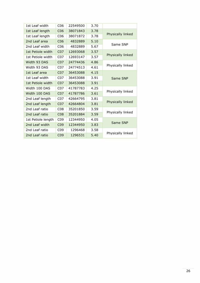
3.4 Physically linked SNPs and SNPs associated to several traits

In fifteen cases, SNPs associated to the same trait were physically linked. Also in nine cases

the same SNP was associated to several traits. This was the case for SNPs linked to both

number of leafs and total number of leafs, which was expected, but also with leaf area and

leaf width. These physically linked SNPs and SNPs associated to several traits are shown in

Table 9.

Table 9. Significant SNPs associated to traits that are physically linked to each other or the

same SNPs found to be associated to several traits. The last column shows which SNPs,

physically linked to each other, are associated to the same traits or which SNPs are found to

be associated to several traits.

Trait Chr. Position LOD Same for several

traits /

Physically linked

1st Petiole width C00 1163016 4.62 Physically linked

1st Petiole width C00 1163028 4.62

2nd Leaf ratio C00 20327423 3.86

Physically linked 2nd Leaf ratio C00 20327444 3.86

2nd Leaf ratio C00 20327465 3.86

2nd Leaf ratio C00 20327475 3.86

Number of Leafs C00 3171193 3.58 Same SNP

Total # Leafs C00 3171193 3.82

Number of Leafs C00 3171195 3.58 Same SNP

Total # Leafs C00 3171195 3.82

2nd Leaf area C00 75750776 3.88 Same SNP

2nd Leaf width C00 75750776 3.80


2nd Leaf width C00 75809874 5.43



1st Leaf width C02 17100721 3.89 Physically linked

1st Leaf width C02 17100748 3.62

2nd Leaf width C02 32271087 3.88

Physically linked 2nd Leaf width C02 32271126 3.91

2nd Leaf width C02 32271129 3.90

2nd Leaf width C02 32271132 4.33

1st Leaf area C03 33828976 3.62 Same SNP

1st Leaf width C03 33828976 3.70

1st Leaf ratio C03 52331254 3.73 Physically linked

1st Leaf ratio C03 52331287 3.73

Number of Leafs C05 15904347 3.63 Physically linked

Number of Leafs C05 15904460 3.65

Number of Leafs C06 11671229 4.10 Physically linked

Number of Leafs C06 11671280 3.83

1st Leaf area C06 22549500 3.57 Same SNP

26

1st Leaf width C06 22549500 3.70

1st Leaf length C06 38071843 3.78 Physically linked

1st Leaf length C06 38071872 3.78


2nd Leaf width C06 4832889 5.67



Width 93 DAS C07 24774436 4.86 Physically linked

Width 93 DAS C07 24774513 4.61

1st Leaf area C07 36453088 4.15

Same SNP 1st Leaf width C07 36453088 3.91


Width 100 DAS C07 41787783 4.25 Physically linked

Width 100 DAS C07 41787786 3.61

2nd Leaf length C07 42664795 3.81 Physically linked

2nd Leaf length C07 42664804 3.81

2nd Leaf ratio C08 35201850 3.59 Physically linked

2nd Leaf ratio C08 35201884 3.59

1st Petiole length C09 12344950 4.05 Same SNP

2nd Leaf width C09 12344950 3.83

2nd Leaf ratio C09 1296468 3.58 Physically linked

2nd Leaf ratio C09 1296531 5.40

27

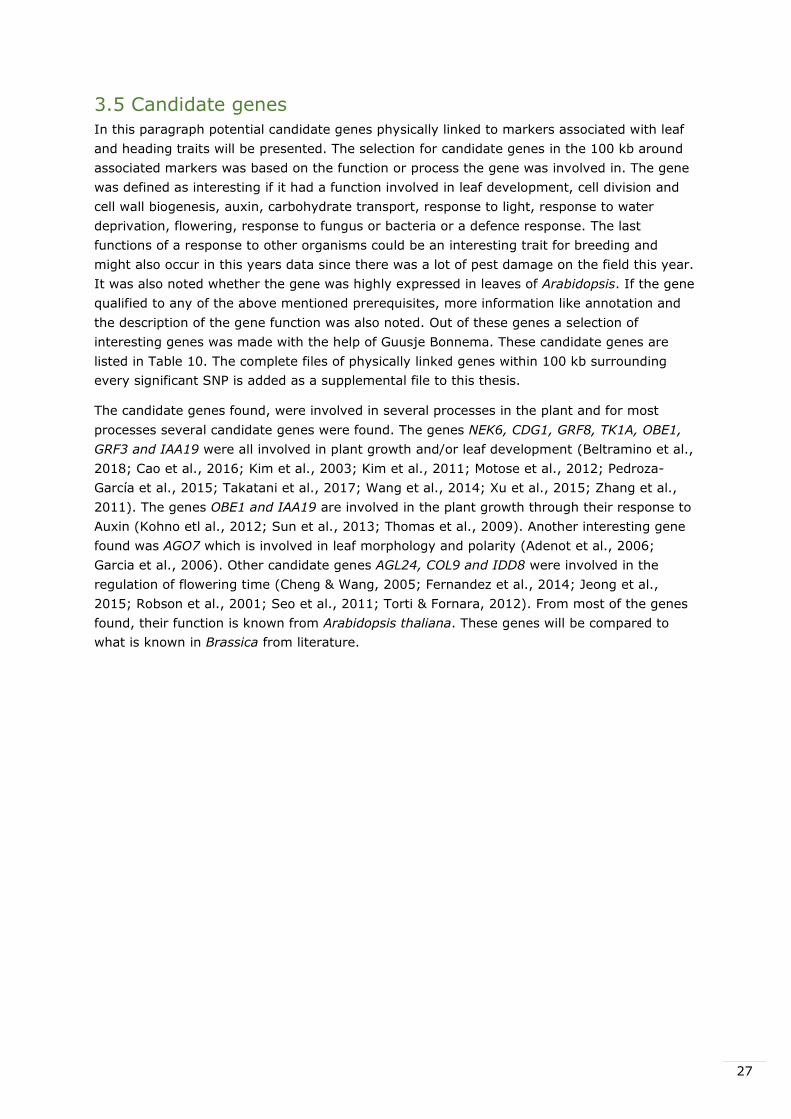
3.5 Candidate genes

In this paragraph potential candidate genes physically linked to markers associated with leaf

and heading traits will be presented. The selection for candidate genes in the 100 kb around

associated markers was based on the function or process the gene was involved in. The gene

was defined as interesting if it had a function involved in leaf development, cell division and

cell wall biogenesis, auxin, carbohydrate transport, response to light, response to water

deprivation, flowering, response to fungus or bacteria or a defence response. The last

functions of a response to other organisms could be an interesting trait for breeding and

might also occur in this years data since there was a lot of pest damage on the field this year.

It was also noted whether the gene was highly expressed in leaves of Arabidopsis. If the gene

qualified to any of the above mentioned prerequisites, more information like annotation and

the description of the gene function was also noted. Out of these genes a selection of

interesting genes was made with the help of Guusje Bonnema. These candidate genes are

listed in Table 10. The complete files of physically linked genes within 100 kb surrounding

every significant SNP is added as a supplemental file to this thesis.

The candidate genes found, were involved in several processes in the plant and for most

processes several candidate genes were found. The genes NEK6, CDG1, GRF8, TK1A, OBE1,

GRF3 and IAA19 were all involved in plant growth and/or leaf development (Beltramino et al.,

2018; Cao et al., 2016; Kim et al., 2003; Kim et al., 2011; Motose et al., 2012; Pedroza-

García et al., 2015; Takatani et al., 2017; Wang et al., 2014; Xu et al., 2015; Zhang et al.,

2011). The genes OBE1 and IAA19 are involved in the plant growth through their response to

Auxin (Kohno etl al., 2012; Sun et al., 2013; Thomas et al., 2009). Another interesting gene

found was AGO7 which is involved in leaf morphology and polarity (Adenot et al., 2006;

Garcia et al., 2006). Other candidate genes AGL24, COL9 and IDD8 were involved in the

regulation of flowering time (Cheng & Wang, 2005; Fernandez et al., 2014; Jeong et al.,

2015; Robson et al., 2001; Seo et al., 2011; Torti & Fornara, 2012). From most of the genes

found, their function is known from Arabidopsis thaliana. These genes will be compared to

what is known in Brassica from literature.

28

Table 10. Candidate genes physically linked to SNPs associated to leaf and cabbage head traits and the reference in which the gene is described in literature. Trait Chr Pos LOD Name Involved in Reference(s)

Leaf area & Leaf width

C03 C03

33828976 33828976

3.62 3.70

NEK6 These results suggest that NEK6, NIMA-related kinase 6, promotes directional cell growth (Takatani et al., 2017). It is suggested that plant NEKs function in directional cell growth and organ development (Motose et al., 2012). Here we report functions of NEK6 in plant growth, development and stress responses in Arabidopsis (Zhang et al., 2011).

Motose et al., 2012; Takatani et al., 2017; Zhang et al., 2011

Leaf length

C07 C07

26014987 26015016

3.96 3.96

CDG1 Transgenic experiments confirm that CDG1 (Constitutive Differential Growth 1) and its homolog CDL1 positively regulate brassinosteroid signalling and plant growth.

Kim et al., 2011

Leaf length

C07 43455384 3.83 GRF8 Over-expression of BrGRF8 (Brassica rapa Growth Regulating Factor 8) in transgenic Arabidopsis plants increased the sizes of the leaves and other organs by regulation of cell proliferation (Wang et al., 2014) The GRF proteins of A. thaliana are involved in regulating the growth and development of leaves (Kim et al., 2003).

Kim et al., 2003; Wang et al., 2014

Leaf length

C07 43455384 3.83 AGL24 AGL15 (Agamous-Like) and AGL18, along with SVP and AGL24, are necessary to block initiation of floral programs in vegetative organs (Fernandez et al., 2014). It is suggested that flowering is controlled by AGL24 partly independently of SOC1 and FUL (Torti & Fornara, 2012).

Fernandez et al., 2014; Torti & Fornara, 2012

Width 93 DAS

C07 C07

24774436 24774513

4.86 4.61

Leaf development TAIR, 2018

Width 93 DAS

C01 38380783 4.07 PRA1.B3 Different AtPRA1 (A. thaliana Prenylated Rab Acceptor) family members displayed distinct expression patterns, with a preference for vascular cells and expanding or developing tissues. AtPRA1 genes were significantly co-expressed with Rab GTPases and genes encoding vesicle transport proteins, suggesting an involvement in the vesicle trafficking process.

Kamei et al., 2008

Width 93 DAS

C01 38380783 4.07 NMD3 Nonsemse-Mediated mRNA Decay 3 (NMD3) encodes a protein involved in the nuclear export of the 60S ribosomal subunit and formation of the secondary cell wall.

Chen et al., 2012

Width 93 DAS

C01 38380783 4.07 TK1A

We found that TK1a (Thymidine Kinase 1a) is expressed in most tissues during plant development. Our results suggest that thymidine kinase contributes to several DNA repair pathways (Pedroza-García et al., 2015). Our findings clarify the specialized function of two TKs in A. thaliana and establish that the salvage pathway mediated by the kinases is essential for plant growth and development (Xu et al., 2015).

Pedroza-García et al., 2015; Xu et al. 2015

Width 93 DAS

C01 38380783 4.07 OBE1 The results suggest that OBE (Oberon) proteins have a wider role to play in growth and development. We suggest that OBE1 and OBE2 most likely control the transcription of genes required for auxin responses through the action of their PHD finger domains.

Thomas et al., 2009

Width 93 DAS

C01 38380783 4.07 COL9 Our results indicate that COL9 (Constans-Like 9) is involved in regulation of flowering time by repressing the expression of CO, concomitantly reducing the expression of FT and delaying floral transition

Cheng & Wang, 2005

Width 93 DAS

C01 37407625 3.89 NCED5 We demonstrate that the complex modulates ABA levels in Arabidopsis exposed to cold and high salt by differentially controlling NCED3 and NCED5 (Nine-Cis-Epoxycarotenoid Dioxygenase 5) mRNAs turnover, which represents a new layer of regulation in the biosynthesis of this phytohormone in response to abiotic stress (Perea-Resa et al., 2016). NCED5 thus contributes, together with NCED3, in ABA production affecting plant growth and water stress tolerance (Frey et al., 2012).

Frey et al., 2012; Perea-Resa et al., 2016

Width 93 DAS

C04 4342466 3.87 GRF3 Introduction of At-rGRF3 (Growth-Regulating Factor) in Brassica oleracea can increase organ size, and when At-rGRF3 homologs from soybean and rice are introduced in Arabidopsis, leaf size is also increased. This suggests that regulation of GRF3 activity by miR396 is important for organ growth in a broad range of species (Beltramino et al., 2018). Growth-regulating factors (GRFs) are plant-specific transcription factors that have important functions in regulating plant growth and development (Cao et al., 2016).

Beltramino et al., 2018; Cao et al., 2016

Width 93 DAS

C04 4342466 3.87 HARDY Overexpression of HARDY, an AP2/ERF gene from Arabidopsis, improves drought and salt tolerance by reducing transpiration and sodium uptake in transgenic Trifolium alexandrinum L (Abogadallah et al., 2011) Improvement of water use efficiency in rice by expression of HARDY, an Arabidopsis drought and salt tolerance gene (Karaba et al., 2007)

Abogadallah et al., 2011; Karaba et al., 2007

Width 93 DAS

C06 19958883 3.66 IDD8 The Indeterminate Domain (IDD)-containing transcription factor IDD8 regulates flowering time by modulating sugar metabolism and transport under sugar-limiting conditions in Arabidopsis (Jeong et al., 2015). We demonstrate that AtIDD8 regulates photoperiodic flowering by modulating sugar transport and metabolism (Seo et al., 2011).

Jeong et al., 2015; Seo et al., 2011

Width 93 DAS

C06 C06

19958883 19958883

3.66 3.66

KINESIN-13A

We demonstrate here that the internal-motor kinesin AtKINESIN-13A (AtKIN13A) limits cell expansion and cell size in Arabidopsis thaliana, with loss-of-function atkin13a mutants forming larger petals with larger cells.

Fujikura et al., 2014

29

Width 93 DAS

C02 21802598 3.64 PILS The PIN-LIKES (PILS) putative auxin carriers localize to the endoplasmic reticulum (ER) and contribute to cellular auxin homeostasis. PILS proteins regulate intracellular auxin accumulation, the rate of auxin conjugation and, subsequently, affect nuclear auxin signalling.

Feraru et al., 2012

Width 100 DAS

C07 C07

41787783 41787786

4.3 3.6

BAM3 Loss‐of‐function alleles of BAM1 (Barely Any Meristem 1), BAM2 and BAM3 receptors lead to phenotypes consistent

with the loss of stem cells at the shoot and flower meristem. These include a requirement for BAM1, BAM2 and BAM3 in the development of high‐ordered vascular strands within the leaf and a correlated control of leaf shape,

size and symmetry (DeYoung et al., 2006). Here we report that second-site null mutations in the Arabidopsis leucine-rich repeat receptor-like kinase gene BAM3 perfectly suppress the postembryonic root meristem growth defect and the associated perturbed protophloem development of the brevis radix (brx) mutant. The roots of BAM3 mutants specifically resist growth inhibition by the CLE45 peptide ligand (Depuydt et al., 2013).

Depuydt et al., 2013; DeYoung et al., 2006

Weight C02 23618670 3.53 AGO7 DRB4-Dependent TAS3 trans-Acting siRNAs Control Leaf Morphology through AGO7, Argonaute-like7 (Adenot et al., 2006) AGO7 is together with genes ETT, ARF3, ARF4, FIL, RDR6 and SGS3 involved in leaf polarity (Garcia et al., 2006)

Adenot et al., 2006; Garcia et al., 2006

Leafs C01 33540674 3.53 IAA19 Our genetic assays demonstrate that IAA19 (Indole-3-Acetic Acid 19) and IAA29 are sufficient for PIF4 to negatively regulate auxin signaling and phototropism (Sun et al., 2013). Auxin-nonresponsive grape Aux/IAA19 is a positive regulator of plant growth (Kohno et al., 2012).

Kohno et al., 2012; Sun et al., 2013

Scars C08 36021179 4.21 GLK1 ATAF1 represses GLK1 (Golden2-Like 1) expression and shifts the physiological balance towards progression of senescence (Garapati et al., 2015). ORE1 antagonizes GLK1 and 2 transcriptional activity, shifting the balance from chloroplast maintenance towards deterioration (Rauf et al., 2013).

Garapati et al., 2015; Rauf et al., 2013

30

4. Discussion In this chapter the conclusions and recommendations from this thesis will be given. First the

pictures made for the phenotypic data and the Halcon script which is used to analyse these

pictures will be discussed. Secondly there will be a focus on phenotypic data collection. As a

third part the Spearman’s correlation test, to test for correlations between traits will be

discussed. Then the correction for population structure by PCO will be treated. As a fifth part

the GWAS in TASSEL will be discussed and finally the significant SNPs and associated

candidate genes will be treated.

In the field pictures of the leafs of all 404 accessions were made twice and pictures of the

cabbage head was also made once at the harvest of the 137 heading cabbages. In total more

than 3.500 pictures were taken. The advantage of measuring in this way is that a lot of

accessions can be done quickly. The disadvantage is that the pictures are made in 2D. It is

hard to get a correct measurement of the leaf size especially when the leaves are curly or

when leaves or lobes are overlapping. We tried to make this influence as small as possible by

pushing on the leafs to make them as flat as possible. This was mainly necessary for the

savoy cabbage and the tronchuda leafs.

There are several software tools for plant image analysis. For instance ImageJ or Halcon are

being used for these purposes (Abràmoff et al., 2004; Lobet et al., 2013). During this thesis

most pictures were analysed by a Halcon script. A big advantage was that the Halcon script

could recognise the QR-code used and gave accurate values for the leaf parameters

measured. The Halcon script produces a picture with only the leaf in colour and the rest of the

picture in black. With this picture it can be checked if Halcon recognises the leaf properly and

measures the traits correct. All pictures used for analysis were checked manually for their

correctness. In about 90% of the pictures the Halcon script gave good measurements.

Pictures taken on one specific day could not be analysed properly because no blue cloth was

used as a background and therefore the background colour was not even. Other problems

which occurred with analysing the pictures were that for some pictures the Halcon script

included a broad line around the leaf which made the measurements of traits incorrect. For

other pictures the script only recognised part of the leaf and the rest was simply cut off.

These faults could be improved by improving the script on which Halcon is run. This might be

possible by using more reference points on the background in which the Halcon script has

more points of background colour which it recognises as background. Another option would be

to raise the leafs a couple centimetres by putting something under the leaf, just like it was

done with the cabbage head. In this way more light can come under the leaf and less shade is

created directly around the leaf. For the pictures which were not analysed correctly through

the Halcon script it was necessary to analyse them manually with ImageJ. This takes more

time since every picture has to be analysed separately.

For the petiole length and width it is not yet known if Halcon can analyse this properly. During

our research it was tried to indicate where the petiole ends by placing a stick next to the leaf

at this same position. The Halcon script can recognise this stick and can measure where the

petiole ends. At some data the Halcon script seems to give a correct measurement, but with

other pictures this is not the case. For several pictures the petiole width was five times as

high as the petiole length which does not seem realistic. This could be caused by lobes which

sometimes are present on the petiole. Halcon cannot (yet) recognise these lobes and counts it

31

as the petiole. There have been studies in B. rapa which separately measured the number of

lobes and split up the leaf petiole length until the first lobe or until the lamina base (Song et

al., 1995). Also in B. oleracea the number of lobes have been recorded before and the petiole

was measured individually or with auricle’s or wings (Sebastian et al., 2002). Unfortunately

there was not enough time to check the measurements of Halcon towards the petiole

properly, it is recommended to still do this later. Because the petiole data could not be

checked it is not known if this data is reliable and therefore it was not used to find possible

candidate genes.

The Halcon script successfully quantified the white cabbage head images, resulting in values

for cabbage head height, width and area. For the red cabbage head data this was

unfortunately not the case. The script only recognised the white core of the red cabbage and

not the complete red cabbage head. One solution could be to adapt the Halcon script for

background correction. Another option for next year would be to use a different colour of

background which does not look as much like the red (or actually purple) cabbage. If that is

not an option, Image J could be used to manually measure the red cabbage head pictures. For

this thesis it was not possible to use the data of the cabbage heads since the red cabbages

could not be included.

It was not yet possible to measure the core of the cabbage head properly using the Halcon

script. This could be measured with an improved Halcon script, but this would require

advanced script writing. The Halcon script recognises the leaf and cabbage head data because

they have a different colour then the background. With the core being white which looks a lot

like the rest of the leafs of the white cabbage head this would be a lot harder. In all cabbage

head images a red pin was inserted at the top of the core for the white cabbage heads, for the

red cabbage heads this was a yellow pin. The Halcon script must be adapted to recognise this

pin and see this as the end of the core. At this moment there is no expertise in the group to

program the Halcon script in this way. Another option to recognise the core would be to use

3D imaging. In a previous thesis in B. oleracea, 3D imaging is also used after which the core

of the cabbage head could be measured (Groot, 2016).

For all collected phenotypic data the block, date and DAS was noted. It was checked whether

there was a block or a DAS effect. For the dataset of the cabbage head harvest a block and a

DAS effect was found. The last harvest was 13 days later then the first harvest. Therefore

some cabbages had 13 days of extra growth compared to the first harvested cabbages. The

data was not normally distributed so a log transformation was done. There was a block and a

DAS effect found, but the block effect was actually caused by the DAS. Block A was harvested

first and then block B was harvested. A linear model was used with the data of block, DAS

and TKI as fixed factors. A correction was made for the DAS effect and new corrected means

for the traits were calculated. This dataset was used for further analyses. In the datasets of

leaf traits and cabbage width no block or DAS effects were found. This was also expected as

these datasets required less days to score.

A Spearman’s correlation test was used to calculate correlations between the traits measured.

There were some strong positive correlations between leaf length, leaf width and leaf area,

which was expected. There was also a correlation between the width of the cabbage head

measured during growth and the width (0.68 - 0.79) and the weight (0.7 - 0.8) at harvest

stage. In this way it would be possible to measure the width during growth stage and partly

forecast the end width and/or weight of the cabbage head. This could be an interesting

correlation to be used for breeding.

32

Another interesting correlation was found between the leaf width and the width and the

weight of the cabbage head both during growth and at harvest stage. This correlation was

between 0.16 and 0.46 depending on the developmental stages in which leaf and head traits

were phenotyped. For the second leaf width measurement there was a correlation of 0.44 to

the harvested cabbage width, this correlation was between 0.39 and 0.46 for the cabbage

width during growth. The leaf width of the second measurement had a correlation of 0.43 to

the weight of the harvested cabbage head. Especially these correlations ranging between 0.39

and 0.46 could be an interesting trait for breeding. Measuring the width of the largest leaf on

the plant during growth stage could give an indication for the head width and weight at

harvest stage. It would be interesting to investigate this correlation further. Correlations of

leaf width and grain yield were found in rice (Agahi et al., 2007; Ekka, Sarawgi, & Kanwar,

2011). Also in Chinese cabbage (Brassica rapa) correlations between rosette-leaf traits and

both head traits and heading capacity. A positive correlation between leaf width and final

heading degree was found (Sun et al., 2018).

In a previous thesis PCO and STRUCTURE were compared as different methods to correct for

population structure. It was found that PCO had a better correction. Comparisons were also

made between using 10 or 30 axes and it was found that 30 axes worked the best to correct

for population structure (Brouwer, 2018). As a correction method for the population structure

in this thesis also PCO was being used. During this thesis for several datasets PCO’s of 10, 20,

30, 50, 100 and 137 up to 180 axes were tested. The more axes a PCO has, the higher the

percentage of variation it can explain. It was found that the PCO’s with most axes possible for

that dataset, gave the strongest correction. Therefore these PCO’s were used for analyses in

TASSEL. The disadvantage of using these PCO’s with a lot of axes is that they take several

days up to several weeks to run, with 999 permutations, in TASSEL.

Unfortunately PCO can also account for false negatives. It corrects for the population

structure because of different kind of relatedness for the different morphotypes. But variation

of some traits is also associated with the morphotypes. Red cabbages are usually smaller

compared to white cabbages. The markers that will be corrected for may also include the

markers that truly explain this size difference (Korte & Farlow, 2013; Vilhjálmsson &

Nordborg, 2012).

One problem is the occurrence of false positives. This can be caused by SNPs which seem

highly associated but are actually not associated or this can be because of not enough

correction for population structure. The false positives could be accounted for by running

permutations tests. It was also tested to run the TASSEL analyses with 999 permutations like

is done more often in literature with 1000 permutations (Külheim et al., 2011; Müller et al.,

2017). This was also compared with running the data without permutations. It is better to test

the data with more permutations, but because of a limiting time it was sometimes necessary

to run some analyses without any permutations. The GWAS with 999 permutations took

several days up to several weeks to be finished. The population structure and permutations

used will reduce the false positives, but might also result in false negatives.

Nearly all datasets were compared to be run with and without 999 permutations, only for the

dataset of 2nd leaf scoring it was not possible to do both due to a lack of time. In total 83

significant SNPs were found without permutations and 80 significant SNPs were found for the

tests with 999 permutations in all other datasets. These 80 SNPs found with permutations

were associated to a total of 43 leaf and 37 cabbage head traits. Analyses with and without

permutations resulted in the same SNPs associated with traits, even with the same LOD

33

score. The tests without permutations only gave three additional probably false positives

(3.6%) for the trait total number of leafs, for all other traits no difference could be found.

Although differences seem small, I still recommended to run the datasets with permutations.

Analyses could first be run without permutations to start the rest of the work after the GWAS.

In this way the other work can already be done while the GWAS with 999 or 1000

permutations is still running. Unfortunately no literature could be found which compared

running a GWAS in TASSEL with and without permutations so no comparisons to other articles

could be made.

For the 3rd measurement of the cabbage head width at 105 DAS it was not possible to analyse

this in a GWAS, since an error in TASSEL kept occurring. The exact reason of this error is not

yet known because the same PCO and genotypic data was used during the other two

measurements. The phenotypic data was in the exact same format as the two measurements

before. The only difference was that only 143 accessions were phenotyped at 105 DAS

compared to 174 and 160 at 93 and 100 DAS. Since a PCO calculated over the 180 heading

cabbage accessions was used, this might be the reason why the error kept occurring.

Most previous theses in B. oleracea used a LD of 50 kb (Islam, 2017; Topper, 2016; van

Eggelen, 2017). Brouwer found a LD of 150 kb during his thesis. He calculated the linkage

disequilibrium in his own SNP dataset, which is the same dataset which is being used this year

(Brouwer, 2018). In a mixed population of B. oleracea consisting of the morphotypes Chinese

kale, broccoli, cauliflower, kohlrabi, wild oleracea, Brussels sprouts, kale and cabbage the

averaged LD calculated over the whole population was 36.8 kb. The LD of only the cabbages

was also calculated in the same paper and retrieved from a figure this was estimated to be 50

kb (Cheng et al., 2016). In this research also a LD of 50 kb was taken. Some genetic regions

have a higher chance of recombination and therefore a lower LD and other regions have it the

other way around, therefore a pragmatic solution is to use an average LD of 50 kb.

For the significant SNPs, genes within 100 kb were found in the brassica genome browser

(BRAD, 2018). Unfortunately this was not possible for the 24 SNPs located on chromosome 0.

These SNPs represent scaffolds with an unknown chromosomal location. A better genome of

B. oleracea is generated now, and only for about half a chromosome the exact position is not

yet known compared to nearly two chromosomes in our genotypic data (G. Bonnema & G.

Ning, personal communication on 22-11-2018). It is recommended to try to find the exact

location of these SNPs, by mapping the GBS reads to this new genome because they might

also be located near important candidate genes.

For the other SNPs of which their location was known, orthologues of the genes found in the

brassica genome browser were found in the Arabidopsis genome browser (TAIR, 2018).

Annotation of Arabidopsis thaliana orthologues can give information about the function of the

gene and it’s expression pattern. For the genes which had an interesting function or where

highly expressed in leafs of A. thaliana more information was found. This included other gene

names and a description of the gene. With all this information it was still hard to determine

which genes are the likely candidates explaining the variation for the SNPs found. For some

SNPs no genes were found, and for other SNPs up to 24 different genes were found. Most of

these genes were highly expressed in leafs. Several of the genes were involved in leaf

development, leaf senescence or other influences on the field like temperature or drought

which would also make sense. With help of Guusje Bonnema the most interesting candidate

genes were selected and investigated further. For these specific candidate genes a literature

review was done to find out if references were available which described the genes.

34

All candidate genes are shown in Table 10. Some of these will be covered here in the

discussion. A significant SNP which was found at the 93 DAS measurement of the cabbage

head width on chromosome 1, position 38380783, was close to the gene Thymidine Kinase 1a

(TK1a). The A. thaliana genome has two different TK’s (AtTK1 and AtTK2) and it is shown that

the salvage pathway mediated by the kinases is essential for plant growth and development

(Xu et al., 2015).

Another interesting gene found at the 93 DAS measurement of the cabbage head width was

found at chromosome 4. The Growth-Regulating Factor 3 (GRF3) is known to be involved in

growth. It is even shown that the introduction of At-rGRF3 in B. oleracea can increase organ

size (Beltramino et al., 2018). This gene was also expected to be found for the leaf traits, and

GRF8 was found to be associated to leaf length. The GRF proteins of A. thaliana are involved

in regulating the growth and development of leaves (Kim et al., 2003). Overexpression of

Brassica rapa GRF8 in transgenic Arabidopsis plants increased the sizes of the leaves and

other organs by regulation of cell proliferation (Wang et al., 2014). GRF5 is found to be

associated to lamina length, petiole length, leaf index and plant mature height in B. rapa

(Xiao et al., 2014). The BraA.GRF14 genes showed distinct expression pattern during plant

developmental stages in B. rapa (Chandna et al., 2016).

For the width at 93 DAS on chromosome 1 also the gene Constans-Like 9 (COL9) was

physically close to a significant associated SNP. COL9 is known to be involved in regulating

flowering time in Arabidopsis (Cheng & Wang, 2005; Robson et al., 2001). For the cabbage

head formation, delay of flowering time is an important characteristic since upon transition to

the generative stage no more leafs are formed. COL4, another gene from the same Constans-

like gene family was also identified in a previous thesis, as a candidate gene associated with

core length and mean width mature leaf (Brouwer, 2018). COL5 is found in the thesis of

Topper as a candidate gene to be associated to head weight (Topper, 2016). A quantitative

trait nucleotide (QTN) affecting flowering time is located within or close to the Bni COL1 gene

in B. nigra (Österberg et al., 2002).

A SNP significantly associated with number of leafs at chromosome 1, 35 kb from the gene

IAA19 (Indole-3-Acetic Acid 19) was found. IAA19 was also found to be associated to petiole

area, total area and mean width leaf in the thesis of Brouwer and associated to head weight in

the thesis of van Eggelen (Brouwer, 2018; van Eggelen, 2017). IAA3 and IAA19 are known to

be expressed in the ornamental B. oleracea var. acephala f. tricolor (Xie et al., 2014).

Brassica rapaIAA2, BrIAA19 and BrIAA29 were found as auxin-dependent shade-induced

genes (Procko et al., 2014).

It is still needed to validate the candidate genes found. As a start the effect of the linked SNP

could be found by comparing the trait values of accessions which have a different allele for

this SNP. After the most interesting candidate genes are selected, markers could be

developed specifically for these genes. This could be done by selecting primers to sequence

the alleles of selected accessions representing the different morphotypes. These sequences

would need to be aligned and possible paralogues could be found. Then cleaved amplified

polymorphic sequence (CAPS) markers could be developed. These CAPS markers could

confirm the association of the gene to the trait. This was also done for B. oleracea in previous

theses (Báez, 2018; Pirzada, 2018).

35

In conclusion, phenotypic and genotypic data was combined together with a PCO to correct for

population structure and a GWAS was done in TASSEL. In total 115 significant SNPs were

found associated to various leaf and head traits. Potential genes of interest within 100 kb of

the SNP were found. From all genes found, a shortlist was made with the potential genes of

interest. For these genes a literature review was done and a shortlist was made on candidate

genes which may be involved in leaf and head formation of B. oleracea.

36

References Abogadallah, G. M., Nada, R. M., Malinowski, R., & Quick, P. (2011). Overexpression of

HARDY, an AP2/ERF gene from Arabidopsis, improves drought and salt tolerance by

reducing transpiration and sodium uptake in transgenic Trifolium alexandrinum L. Planta, 233(6), 1265–1276. https://doi.org/10.1007/s00425-011-1382-3

Abràmoff, M. D., Hospitals, I., Magalhães, P. J., & Abràmoff, M. (2004). Image

Processing with ImageJ. Biophotonics International, 11(7), 7.

https://doi.org/10.1201/9781420005615.ax4

Adenot, X., Elmayan, T., Lauressergues, D., Boutet, S., Bouché, N., Gasciolli, V., &

Vaucheret, H. (2006). DRB4-Dependent TAS3 trans-Acting siRNAs Control Leaf

Morphology through AGO7. Current Biology, 16(9), 927–932. https://doi.org/10.1016/j.cub.2006.03.035

Agahi, K., Fotokiann, M. H., & Farshadfar, E. (2007). Correlation and Path Coefficient

Analysis for Some Yield-Related Traits in Rice Genotypes (Oryza sativa L.). Asian Journal of Plant Sciences, 6, 513–517.

auf’m Erley, G. S., Dewi, E. R., Nikus, O., & Horst, W. J. (2010). Genotypic differences in

nitrogen efficiency of white cabbage (Brassica oleracea L.). Plant and Soil, 328(1), 313–325. https://doi.org/10.1007/s11104-009-0111-1

Báez, J. A. (2018). Approach in the development and evaluation of DNA molecular

markers in Brassica species. Wageningen University Thesis.

Beltramino, M., Ercoli, M. F., Debernardi, J. M., Goldy, C., Rojas, A. M. L., Nota, F., …

Rodriguez, R. E. (2018). Robust increase of leaf size by Arabidopsis thaliana GRF3-

like transcription factors under different growth conditions. Scientific Reports, 8(1), 1–13. https://doi.org/10.1038/s41598-018-29859-9

Benrey, B., & Denno, R. F. (1997). The Slow-Growth-High-Mortality Hypothesis: a Test

Using the Cabbage Butterfly. Ecology, 78(4), 987–999.

Bonnema, G., Del Carpio, D. P., & Zhao, J. (2011). Diversity Analyss and Molecular

Taxonomy of Brassica Vegetable Crops. Genetics, Genomics and Breeding of Vegetable Brassicas, 81–124.

BRAD. (2018). Brassica Genome Browse. Retrieved December 6, 2018, from http://brassicadb.org/cgi-bin/gbrowse/Oleracea/

Bradbury, P. J., Zhang, Z., Kroon, D. E., Casstevens, T. M., Ramdoss, Y., & Buckler, E. S.

(2007). TASSEL: Software for association mapping of complex traits in diverse

samples. Bioinformatics, 23(19), 2633–2635. https://doi.org/10.1093/bioinformatics/btm308

Branca, F., & Cartea, E. (2011). Brassica. Wild Crop Relatives: Genomic and Breeding Resources, 17–36. https://doi.org/10.1007/978-3-642-14871-2

Brouwer, H. (2018). Genetic Analysis on Brassica oleracea breeding traits. Wageningen

University Thesis.

Cao, Y., Han, Y., Jin, Q., Lin, Y., & Cai, Y. (2016). Comparative Genomic Analysis of the

GRF Genes in Chinese Pear (Pyrus bretschneideri Rehd), Poplar (Populous), Grape

(Vitis vinifera), Arabidopsis and Rice (Oryza sativa). Frontiers in Plant Science, 7, 1–14. https://doi.org/10.3389/fpls.2016.01750

Cartea, M. E., Lema, M., Francisco, M., & Velasco, P. (2011). Basic information on

vegetable Brassica crops. Genetics, Genomics and Breeding of Vegetable Brassicas, 1–33. https://doi.org/doi:10.1201/b10880-2\r10.1201/b10880-2

Chandna, R., Augustine, R., Kanchupati, P., Kumar, R., Kumar, P., Arya, G. C., & Bisht,

N. C. (2016). Class-specific evolution and transcriptional differentiation of 14-3-3

family members in mesohexaploid Brassica rapa. Frontiers in Plant Science, 7, 1–15.

https://doi.org/10.3389/fpls.2016.00012

Chen, M. Q., Zhang, A. H., Zhang, Q., Zhang, B. C., Nan, J., Li, X., … Bai, S. N. (2012).

Arabidopsis NMD3 is required for nuclear export of 60S ribosomal subunits and

affects secondary cell wall thickening. PLoS ONE, 7(4), 1–14.

37

https://doi.org/10.1371/journal.pone.0035904

Cheng, F., Sun, R., Hou, X., Zheng, H., Zhang, F., Zhang, Y., … Wang, X. (2016).

Subgenome parallel selection is associated with morphotype diversification and

convergent crop domestication in Brassica rapa and Brassica oleracea. Nature Genetics, 48(10), 1218–1224. https://doi.org/10.1038/ng.3634

Cheng, X. F., & Wang, Z. Y. (2005). Overexpression of COL9, a CONSTANS-LIKE gene,

delays flowering by reducing expression of CO and FT in Arabidopsis thaliana. The

Plant Journal, 43(5), 758–768. https://doi.org/10.1111/j.1365-313X.2005.02491.x

Del Carpio, D. P., Basnet, R. K., De Vos, R. C. H., Maliepaard, C., Paulo, M. J., &

Bonnema, G. (2011). Comparative Methods for Association Studies: A Case Study

on Metabolite Variation in a Brassica rapa Core Collection. PLoS ONE, 6(5), 1–10. https://doi.org/10.1371/journal.pone.0019624

Depuydt, S., Rodriguez-Villalon, A., Santuari, L., Wyser-Rmili, C., Ragni, L., & Hardtke,

C. S. (2013). Suppression of Arabidopsis protophloem differentiation and root

meristem growth by CLE45 requires the receptor-like kinase BAM3. Proceedings of

the National Academy of Sciences, 110(17), 7074–7079.

https://doi.org/10.1073/pnas.1222314110

DeYoung, B. J., Bickle, K. L., Schrage, K. J., Muskett, P., Patel, K., & Clark, S. E. (2006).

The CLAVATA1-related BAM1, BAM2 and BAM3 receptor kinase-like proteins are

required for meristem function in Arabidopsis. The Plant Journal, 45(1), 1–16. https://doi.org/10.1111/j.1365-313X.2005.02592.x

Earl, D. A., & VonHoldt, B. M. (2012). STRUCTURE HARVESTER: A website and program

for visualizing STRUCTURE output and implementing the Evanno method.

Conservation Genetics Resources, 4(2), 359–361. https://doi.org/10.1007/s12686-011-9548-7

Ekka, R. E., Sarawgi, A. K., & Kanwar, R. R. (2011). Correlation and path analysis in

traditional rice accessions of Chhattisgarh. Journal of Rice Research, 4(1 & 2), 11–

18.

Evanno, G., Regnaut, S., & Goudet, J. (2005). Detecting the number of clusters of

individuals using the software STRUCTURE: A simulation study. Molecular Ecology, 14(8), 2611–2620. https://doi.org/10.1111/j.1365-294X.2005.02553.x

FAOSTAT. (2018). FAOSTAT. Retrieved June 6, 2018, from http://www.fao.org/faostat/en/#data/QC

Feraru, E., Vosolsobe, S., Feraru, M. I., Petrasek, J., & Kleine-Vehn, J. (2012). Evolution

and structural diversification of PILS putative auxin carriers in plants. Frontiers in Plant Science, 3, 1–13. https://doi.org/10.3389/fpls.2012.00227

Fernandez, D. E., Wang, C.-T., Zheng, Y., Adamczyk, B. J., Singhal, R., Hall, P. K., &

Perry, S. E. (2014). The MADS-Domain Factors AGAMOUS-LIKE15 and AGAMOUS-

LIKE18, along with SHORT VEGETATIVE PHASE and AGAMOUS-LIKE24, Are

Necessary to Block Floral Gene Expression during the Vegetative Phase. Plant Physiology, 165(4), 1591–1603. https://doi.org/10.1104/pp.114.242990

Frey, A., Effroy, D., Lefebvre, V., Seo, M., Perreau, F., Berger, A., … Marion-Poll, A.

(2012). Epoxycarotenoid cleavage by NCED5 fine-tunes ABA accumulation and

affects seed dormancy and drought tolerance with other NCED family members. The

Plant Journal, 70(3), 501–512. https://doi.org/10.1111/j.1365-313X.2011.04887.x

Fujikura, U., Elsaesser, L., Breuninger, H., Sánchez-Rodríguez, C., Ivakov, A., Laux, T., …

Lenhard, M. (2014). Atkinesin-13A Modulates Cell-Wall Synthesis and Cell Expansion

in Arabidopsis thaliana via the THESEUS1 Pathway. PLOS Genetics, 10(9), 1–15. https://doi.org/10.1371/journal.pgen.1004627

Garapati, P., Xue, G. P., Munné-Bosch, S., & Balazadeh, S. (2015). Transcription Factor

ATAF1 in Arabidopsis Promotes Senescence by Direct Regulation of Key Chloroplast

Maintenance and Senescence Transcriptional Cascades. Plant Physiology, 168(3), 1122–1139. https://doi.org/10.1104/pp.15.00567

Garcia, D., Collier, S. A., Byrne, M. E., & Martienssen, R. A. (2006). Specification of Leaf

Polarity in Arabidopsis via the trans-Acting siRNA Pathway. Current Biology, 16(9),

38

933–938. https://doi.org/10.1016/j.cub.2006.03.064

Gray, A. R. (1982). Taxonomy and Evolution of Broccoli (Brassica oleracea var. italica).

Economic Botany, 36(4), 397–410.

Groot, T. (2016). Genetic analysis of heading cabbage traits. Wageningen University Thesis.

Islam, M. (2017). Association Study on Leaf Morphology in a Diverse Collection of Brassica Oleracea. Wageningen University Thesis.

Jeong, E. Y., Seo, P. J., Woo, J. C., & Park, C. M. (2015). AKIN10 delays flowering by

inactivating IDD8 transcription factor through protein phosphorylation in

Arabidopsis. BMC Plant Biology, 15(1), 1–13. https://doi.org/10.1186/s12870-015-0503-8

Kalloo, G., & Bergh, B. O. (1993). Genetic Improvement of Vegetable Crops (1st ed.). Oxford: Pergamon Press.

Kalve, S., De Vos, D., & Beemster, G. T. S. (2014). Leaf development: a cellular

perspective. Frontiers in Plant Science, 5, 1–25.


Kamei, C. L. A., Boruc, J., Vandepoele, K., Van den Daele, H., Maes, S., Russinova, E., …

De Veylder, L. (2008). The PRA1 Gene Family in Arabidopsis. Plant Physiology, 147(4), 1735–1749. https://doi.org/10.1104/pp.108.122226

Karaba, A., Dixit, S., Greco, R., Aharoni, A., Trijatmiko, K. R., Marsch-Martinez, N., …

Pereira, A. (2007). Improvement of water use efficiency in rice by expression of

HARDY, an Arabidopsis drought and salt tolerance gene. Proceedings of the National

Academy of Sciences, 104(39), 15270–15275. https://doi.org/10.1073/pnas.0707294104

Kennard, W. C., Slocum, M. K., Figdore, S. S., & Osborn, T. C. (1994). Genetic analysis

of morphological variation in Brassica oleracea using molecular markers. Theoretical

and Applied Genetics., 87(6), 721–732. https://doi.org/10.1007/BF00222898

Kim, J. H., Choi, D., & Kende, H. (2003). The AtGRF family of putative transcription

factors is involved in leaf and cotyledon growth in Arabidopsis. The Plant Journal, 36(1), 94–104. https://doi.org/10.1046/j.1365-313X.2003.01862.x

Kim, T. W., Guan, S., Burlingame, A. L., & Wang, Z. Y. (2011). The CDG1 Kinase

Mediates Brassinosteroid Signal Transduction from BRI1 Receptor Kinase to BSU1

Phosphatase and GSK3-like Kinase BIN2. Molecular Cell, 43(4), 561–571. https://doi.org/10.1016/j.molcel.2011.05.037

Kohno, M., Takato, H., Horiuchi, H., Fujita, K., & Suzuki, S. (2012). Auxin-nonresponsive

grape Aux/IAA19 is a positive regulator of plant growth. Molecular Biology Reports, 39(2), 911–917. https://doi.org/10.1007/s11033-011-0816-0

Korte, A., & Farlow, A. (2013). The advantages and limitations of trait analysis with

GWAS : a review. Plant Methods, 9(29), 1–9.

Külheim, C., Yeoh, S. H., Wallis, I. R., Laffan, S., Moran, G. F., & Foley, W. J. (2011).

The molecular basis of quantitative variation in foliar secondary metabolites in

Eucalyptus globulus. New Phytologist, 191(4), 1041–1053. https://doi.org/10.1111/j.1469-8137.2011.03769.x

Lan, T. H., & Paterson, A. H. (2001). Comparative mapping of QTLs determining the plant

size of Brassica oleracea. Theoretical and Applied Genetics, 103(2–3), 383–397. https://doi.org/10.1007/s001220100615

Landis, N. (2013). Kale, Broccoli, Brussels Sprouts, and Cabbage are All the Same

Species. Retrieved May 17, 2018, from https://www.foodbeast.com/news/kale-broccoli-brussels-sprouts-and-cabbage-are-all-from-the-same-family/

Li, J., & Ji, L. (2005). Adjusting multiple testing in multilocus analyses using the

eigenvalues of a correlation matrix. Heredity, 95(3), 221–227. https://doi.org/10.1038/sj.hdy.6800717

Liu, S., Liu, Y., Yang, X., Tong, C., Edwards, D., Parkin, I. A. P., … Paterson, A. H.

(2014). The brassica oleracea genome reveals the asymmetrical evolution of

39

polyploid genomes. Nature Communications, 5.

https://doi.org/10.1038/ncomms4930

Lobet, G., Draye, X., & Périlleux, C. (2013). An online database for plant image analysis software tools. Plant Methods, 9(38), 7. https://doi.org/10.1186/1746-4811-9-38

Lv, H., Wang, Q., Han, F., Liu, X., Fang, Z., Yang, L., … Zhang, Y. (2017). Genome-wide

indel/SSR scanning reveals significant loci associated with excellent agronomic traits

of a cabbage (Brassica oleracea) elite parental line ′01-20′. Scientific Reports, 7, 1–

12. https://doi.org/10.1038/srep41696

Lv, H., Wang, Q., Liu, X., Han, F., Fang, Z., Yang, L., … Zhang, Y. (2016). Whole-

Genome Mapping Reveals Novel QTL Clusters Associated with Main Agronomic Traits

of Cabbage (Brassica oleracea var. capitata L.). Frontiers in Plant Science, 7(July), 1–17. https://doi.org/10.3389/fpls.2016.00989

Lv, H., Wang, Q., Zhang, Y., Yang, L., Fang, Z., Wang, X., … Liu, B. (2014). Linkage map

construction using InDel and SSR markers and QTL analysis of heading traits in

Brassica oleracea var. capitata L. Molecular Breeding, 34(1), 87–98. https://doi.org/10.1007/s11032-014-0019-1

Motose, H., Takatani, S., Ikeda, T., & Takahashi, T. (2012). NIMA-related kinases

regulate directional cell growth and organ development through microtubule function

in Arabidopsis thaliana. Plant Signaling and Behavior, 7(11), 1552–1555. https://doi.org/10.4161/psb.22412

Müller, M., Seifert, S., & Finkeldey, R. (2017). Comparison and confirmation of SNP-bud

burst associations in European beech populations in Germany. Tree Genetics and

Genomes, 13(59), 1–12. https://doi.org/10.1007/s11295-017-1145-9

Nagaharu, U. (1935). Genome analysis in Brassica with special reference to the

experimental formation of B. napus and peculiar mode of fertilication. Journal of Japanese Botany, 7, 389–452.

Österberg, M. K., Shavorskaya, O., Lascoux, M., & Lagercrantz, U. (2002). Naturally

occurring indel variation in the Brassica nigra COL1 gene is associated with variation

in flowering time. Genetics Society of America, 161, 299–306. https://doi.org/10.1007/bf02191594

Pang, W., Li, X., Choi, S. R., Dhandapani, V., Im, S., Park, M. Y., … Lim, Y. P. (2015).

Development of a leafy Brassica rapa fixed line collection for genetic diversity and

population structure analysis. Molecular Breeding, 35(54), 1–15.

https://doi.org/10.1007/s11032-015-0221-9

Pedroza-García, J. A., Nájera-Martínez, M., de la Paz Sanchez, M., & Plasencia, J. (2015).

Arabidopsis thaliana thymidine kinase 1a is ubiquitously expressed during

development and contributes to confer tolerance to genotoxic stress. Plant Molecular Biology, 87(3), 303–315. https://doi.org/10.1007/s11103-014-0277-7

Perea-Resa, C., Carrasco-López, C., Catalá, R., Turečková, V., Novak, O., Zhang, W., …

Salinas, J. (2016). The LSM1-7 Complex Differentially Regulates Arabidopsis

Tolerance to Abiotic Stress Conditions by Promoting Selective mRNA Decapping. The Plant Cell, 28(2), 505–520. https://doi.org/10.1105/tpc.15.00867

Pirzada, R. A. (2018). Development of molecular markers for candidate gene profiling in Brassica oleracea for leaf development traits. Wageningen University Thesis.

Pritchard, J. K., Stephens, M., & Donnelly, P. (2000). Inference of Population Structure

Using Multilocus Genotype Data. Genetics Society of America, 155(2), 945–959. https://doi.org/10.1111/j.1471-8286.2007.01758.x

Procko, C., Crenshaw, C. M., Ljung, K., Noel, J. P., & Chory, J. (2014). Cotyledon-

Generated Auxin Is Required for Shade-Induced Hypocotyl Growth in Brassica rapa. Plant Physiology, 165(3), 1285–1301. https://doi.org/10.1104/pp.114.241844

Pulido, A., & Laufs, P. (2010). Co-ordination of developmental processes by small RNAs

during leaf development. Journal of Experimental Botany, 61(5), 1277–1291. https://doi.org/10.1093/jxb/erp397

Rauf, M., Arif, M., Dortay, H., Matallana-Ramírez, L. P., Waters, M. T., Nam, H. G., …

40

Balazadeh, S. (2013). ORE1 balances leaf senescence against maintenance by

antagonizing G2-like-mediated transcription. European Molecular Biology

Organization (EMBO) Reports, 14(4), 382–388. https://doi.org/10.1038/embor.2013.24

Robson, F., Costa, M. M. R., Hepworth, S. R., Vizir, I., Piñeiro, M., Reeves, P. H., …

Coupland, G. (2001). Functional importance of conserved domains in the flowering-

time gene CONSTANS demonstrated by analysis of mutant alleles and transgenic

plants. Plant Journal, 28(6), 619–631. https://doi.org/10.1046/j.1365-313x.2001.01163.x

Sebastian, R. L., Kearsey, M. J., & King, G. J. (2002). Identification of quantitative trait

loci controlling developmental characteristics of Brassica oleracea L. Theoretical and Applied Genetics, 104, 601–609. https://doi.org/10.1007/s001220100743

Seo, P. J., Ryu, J., Kang, S. K., & Park, C. M. (2011). Modulation of sugar metabolism by

an INDETERMINATE DOMAIN transcription factor contributes to photoperiodic

flowering in Arabidopsis. The Plant Journal, 65(3), 418–429.

https://doi.org/10.1111/j.1365-313X.2010.04432.x

Slob, F. (2016). Genetic analysis of leaf morphology in Brassica oleracea. Wageningen University Thesis.

Song, K., Slocum, M. K., & Osborn, T. C. (1995). Molecular marker analysis of genes

controlling morphological variation in Brassica rapa (syn. campestris). Theoretical and Applied Genetics, 90(1), 1–10. https://doi.org/10.1007/BF00220989

Sun, J., Qi, L., Li, Y., Zhai, Q., & Li, C. (2013). PIF4 and PIF5 Transcription Factors Link

Blue Light and Auxin to Regulate the Phototropic Response in Arabidopsis. The Plant Cell, 25(6), 2102–2114. https://doi.org/10.1105/tpc.113.112417

Sun, X., Luo, S., Luo, L., Wang, X., Chen, X., Lu, Y., … Bonnema, G. (2018). Genetic

Analysis of Chinese Cabbage Reveals Correlation Between Rosette Leaf and Leafy

Head Variation. Frontiers in Plant Science, 9, 1–10.


TAIR. (2018). The Arabidopsis Information Resource. Retrieved December 6, 2018, from https://www.arabidopsis.org/

Takatani, S., Ozawa, S., Yagi, N., Hotta, T., Hashimoto, T., Takahashi, Y., … Motose, H.

(2017). Directional cell expansion requires NIMA-related kinase 6 (NEK6)-mediated

cortical microtubule destabilization. Scientific Reports, 7, 1–18.

https://doi.org/10.1038/s41598-017-08453-5

Thomas, C. L., Schmidt, D., Bayer, E. M., Dreos, R., & Maule, A. J. (2009). Arabidopsis

plant homeodomain finger proteins operate downstream of auxin accumulation in

specifying the vasculature and primary root meristem. The Plant Journal, 59(3), 426–436. https://doi.org/10.1111/j.1365-313X.2009.03874.x

Topper, F. (2016). Association Mapping of Leaf Morphology Traits in Brassica oleracea.

Wageningen University Thesis.

Torti, S., & Fornara, F. (2012). AGL24 acts in concert with SOC1 and FUL during

Arabidopsis floral transition. Plant Signaling and Behavior, 7(10), 1251–1254. https://doi.org/10.4161/psb.21552

van Eggelen, J. (2017). Explaining phenotypical variation by assessing genetic variation in Brassica oleracea. Wageningen University Thesis.

Vilhjálmsson, B. J., & Nordborg, M. (2012). The nature of confounding in genome-wide

association studies. Nature Reviews Genetics, 14(1), 1–2. https://doi.org/10.1038/nrg3382

Wang, F., Li, L., Li, H., Liu, L., Zhang, Y., Gao, J., & Wang, X. (2012). Transcriptome

analysis of rosette and folding leaves in Chinese cabbage using high-throughput RNA

sequencing. Genomics, 99(5), 299–307.

https://doi.org/10.1016/j.ygeno.2012.02.005

Wang, F., Qiu, N., Ding, Q., Li, J., Zhang, Y., Li, H., & Gao, J. (2014). Genome-wide

identification and analysis of the growth-regulating factor family in chinese cabbage

41

(Brassica rapa L. ssp. pekinensis). BMC Genomics, 15(807), 1–12.

https://doi.org/10.3390/ijms161226127

Xiao, D., Wang, H., Basnet, R. K., Zhao, J., Lin, K., Hou, X., & Bonnema, G. (2014).

Genetic Dissection of Leaf Development in Brassica rapa Using a Genetical Genomics

Approach. Plant Physiology, 164(3), 1309–1325. https://doi.org/10.1104/pp.113.227348

Xie, Q., Chen, G., Chen, X., Deng, L., Liu, Q., Zhang, Y., & Hu, Z. (2014). Jointly

silencing BoDWARF, BoGA20ox and BoSP (SELF-PRUNING) produces a novel

miniature ornamental Brassica oleracea var. acephala f. tricolor variety. Molecular Breeding, 34, 99–113. https://doi.org/10.1007/s11032-014-0020-8

Xu, J., Zhang, L., Yang, D. L., Li, Q., & He, Z. (2015). Thymidine kinases share a

conserved function for nucleotide salvage and play an essential role in Arabidopsis

thaliana growth and development. New Phytologist, 208(4), 1089–1103. https://doi.org/10.1111/nph.13530

Yu, J., Pressoir, G., Briggs, W. H., Bi, I. V., Yamasaki, M., Doebley, J. F., … Buckler, E. S.

(2006). A unified mixed-model method for association mapping that accounts for

multiple levels of relatedness. Nature Genetics, 38(2), 203–208. https://doi.org/10.1038/ng1702

Yu, J., Zhao, M., Wang, X., Tong, C., Huang, S., Tehrim, S., … Liu, S. (2013). Bolbase: A

comprehensive genomics database for Brassica oleracea. BMC Genomics, 14, 1–7. https://doi.org/10.1186/1471-2164-14-664

Zhang, B., Chen, H. W., Mu, R. L., Zhang, W. K., Zhao, M. Y., Wei, W., … Zhang, J. S.

(2011). NIMA-related kinase NEK6 affects plant growth and stress response in

Arabidopsis. The Plant Journal, 68, 830–843. https://doi.org/10.1111/j.1365-313X.2011.04733.x

Zhu, C., Gore, M., Buckler, E. S., & Yu, J. (2008). Status and Prospects of Association

Mapping in Plants. The Plant Genome Journal, 1(1), 5–20.

https://doi.org/10.3835/plantgenome2008.02.0089

42

Appendix 1. Overview of the field layout The overview of the field layout can be found in Figure 15. The whole overview with the TKI

numbers per accession can be found in a separate excel file additional to this thesis.

Block B 3 & 4 Block B 1 & 2 Block A 3 & 4 Block A 1 & 2

South Ornamental (22) Kohlrabi (48) Cabbage white (102) Brussels sprouts (48) North

The dijk Cabbage savoy (20) The gate

Cabbage red (44)

Cauliflower (60) Collard green (20)

Cabbage pointed (4)

Cabbage pointed (8) Ornamental (22)

Cabbage white (109) Cabbage pointed (4)

Cabbage white (8) Tronchuda (24)

Brussels sprouts (48) Kohlrabi (46)

Cabbage savoy (20)

Cabbage red (43)

Cauliflower (60)

Collard green (22)

Tronchuda (23) Sprouts (1)

Cabbage white (42)

Cauliflower (26) Cabbage white (30) Kohlrabi (2)

Cauliflower (30)

Figure 15. Overview of the field layout with the number of accessions per morphotype.

43

Appendix 2. Guideline of measuring manually in ImageJ In this appendix a guideline for measuring the leaves or cabbage heads manually in ImageJ is

given. This is not written in a scientific way, but in a way that it is clear for someone to use

the guideline.

ImageJ can be downloaded online. Once installed, open the program.

Press File -> Open and select the image you want to analyse.

In each picture there should be a tag which is of known distance. The tag used this year were

110 x 50 mm and the QR code in the tag was a square of 32 x 32 mm. The scale can be

adjusted towards these known measures.

Pick staight line -> Select width of the QR code -> Analyze -> Set scale ->

Set Known discance: at 32

Set Unit of length: at mm

The Scale should be around 7 pixels/mm

Click the box of Global. This keeps the scale set and makes sure that you only have to do this

step once.

After the scale is set the petiole can be measured. This is also done with the straight line. The

length and the width of the petiole are measured manually in this way. It is handy to do it in

this step since you can still see the colours of the leave and the end of the petiole can be

judged more precisely.

After measuring the petiole the colour treshold is going to be changed. We are going to

change the colours of the pictures to make it easier to analyse the measurements of the leaf.

Select Image -> Adjust -> Color Treshold

Set Hue at: 132 – 153

Set Saturation at: 60 – 255

Set Brightness at the first bar between 60 and 130 (usually 87 was used but in some cases

this needed to be adjusted) and the second bar is set at 237.

Then click on Stack to use these settings on your picture. Don’t close the Color Treshold

window but just minimize it, in this way most settings are saved for later pictures. Only the

bars of the Brightness will still need to be adjusted for later pictures, the other ones stay the

same. The settings mentioned above can be used for most pictures and only need to be

adjusted for some pictures.

Then we are going to make the pictures black and white to make it possible to analyse in

ImageJ. Select Process -> Binary -> Make Binary. You can see that the picture is black and

white now.

Select Edit -> Invert. The black and white parts are switching colours now.

Then you need to select which measurements you want to do. This only has to be done once.

Go to Analyze -> Set measurements. In our research the following boxes where selected:

Area, Standard deviation, Bounding rectangle, Shape descriptors, Fit ellipse, Feret’s diameter

and Display label. Then press OK.

Now we can analyse the leaf or cabbage head. Select Analyze -> analyze particles. Set ‘Size

(mm^2)’ at minimum 3000 to make sure that you only measure the tag and the leaf. A new

window with ‘results’ will open and here the results of the measurement are shown.

After copying these results to a desired file a new picture can be opened and the steps above

can be repeated. As mentioned above already some steps can be skipped since ImageJ keeps

these settings the same for later pictures opened.

44

Appendix 3. Guideline for PCO in DARwin The guideline of how an PCO is calculated will be written in a way in which it is

understandable for the reader, this will not be in a scientific way. First the dissimilarity

between the different accessions which are on the field needs to be calculated. This

dissimilarity needs to be used as input file to calculate the PCO.

The dissimilarity can also be calculated in the program DARwin. This is installed on Johan’s

computer.

Go to the tab dissimilairty -> calculate from allelic data and use the file: ‘SNP populatoin

structure’.

First put all accessions which are in the file to the left with the arrow. Then put all accessions

which are wanted to the right with the arrow.

Click on Save dissimilarity as and then press ok and the dissimilarity will be calculated.

The PCO is also done in the program DARwin. First open this program.

Select Factorial analysis -> analysis.

The dissimilarity file which is needed as input was made in previous steps. This file now needs

to be selected.

Select how many axes you want to have calculated. The more axes are selected, the more %

of the variation is explained.

‘Save factorial coordinates as’ has to be selected. This will be done as a AFT file.

When the figure is displayed identifiers can be added to show morphotype, TKI number, etc. A

new identifier file might need to be made depending on the dataset. The different axes can be

shown in the figure and this figure can also be saved.

45

Appendix 4. Guideline for GWAS in Tassel The Genome Wide Association Studys (GWAS)s of this research was done in the Program

Tassel. The guideline will be written in way in which it is easy to follow all the steps instead of

in a scientific way.

For the GWAS three types of data are needed:

- Genotypic data

- PCO

- Phenotypic data

These data files all need to be inserted in a certain way.

Genotypic data: This is the ‘Genotypic data - 80% GT - 2.5% MAF - 60% missing values -

18.850 SNP.vcf’ file. Nothing has to be adjusted to this file, this file just needs to be imported.

PCO: has to be a text file with tabs delimited which starts in the following way:

<covariate>

<Trait> Axis1 Axis2 etc.->

TKI008 0.050394 0.065680

TKI010 0.020356 0.059508

Etc.

The rest of the information which is in this file (% of variation explained, etc.) all has to be

deleted.

Phenotypic data: This also has to be a text file. The file needs to start in the following way:

<Trait> <Scars> <Leafs> etc.->

TKI008 5.167 17.83

TKI010 5.83 19.67

Etc.

For this file the complete data with all numbers behind the point needs to be added.

After preparing these files they can all be added to Tassel.

File -> open -> select the 3 different files (Genotypic data, PCO & Phenotypic data)

Then the three different files need to be combined to one file.

Select all three files together, press present -> data ->

With missing data: press intersect join

Without missing data: press union join

A new file will appear where all the three files are combined.

Then the analyses can be run. Select the new file in which all three data files (Genotypic data,

PCO & Phenotypic data) were combined. Press Analysis -> Association -> GLM

Select ‘Save file to’ for the genotypic and for the statistics data and give it a clear name to

find back later.

Select the box: ‘Run permutations’, type 999 at number of permutations.

Then press OK and the analyses will run.

When the analyses is finished the genotypic and statistics data file can be opened and the

results can be analysed. At the genotypic file the significant SNP’s can be found per trait. This

data can also be copied and pasted into an excel file to only save the significant SNP’s.

At the statistics file figures can be made as output. For instance a QQ-plot and Manhattan

Plots can be made.

Select the statistics file -> go to Results -> select QQ Plot

-> Select Manhattan Plot

46

Appendix 5. PCO of 180 axes for the heading cabbage

subset In Table 11 the percentage of variation explained per axes for the PCO of 180 axes of the 180

heading cabbage subset is shown.

Table 11. PCO of 180 axes for the heading cabbage subset consisting of 180 accessions. The

percentage of variation explained per axis is shown here.

Axis %

Explained

Axis %

Explained

Axis %

Explained

Axis %

Explained

1 25.8 46 0.43 91 0.19 136 0.04

2 6.71 47 0.43 92 0.19 137 0.04

3 4.66 48 0.42 93 0.18 138 0.03

4 3.72 49 0.42 94 0.18 139 0.03

5 2.78 50 0.4 95 0.17 140 0.03

6 2.28 51 0.4 96 0.17 141 0.03

7 2.01 52 0.39 97 0.16 142 0.02

8 1.8 53 0.38 98 0.16 143 0.02

9 1.71 54 0.37 99 0.16 144 0.02

10 1.31 55 0.37 100 0.15 145 0.02

11 1.27 56 0.36 101 0.15 146 0.01

12 1.2 57 0.35 102 0.14 147 0.01

13 1.1 58 0.35 103 0.14 148 0.01

14 1.04 59 0.35 104 0.14 149 0.01

15 0.98 60 0.34 105 0.14 150 0

16 0.97 61 0.33 106 0.13 151 0

17 0.94 62 0.32 107 0.13 152

18 0.88 63 0.32 108 0.13 153

19 0.85 64 0.31 109 0.12 154

20 0.83 65 0.3 110 0.12 155

21 0.81 66 0.3 111 0.11 156

22 0.79 67 0.3 112 0.11 157

23 0.76 68 0.29 113 0.11 158

24 0.75 69 0.29 114 0.11 159

25 0.73 70 0.28 115 0.1 160

26 0.71 71 0.28 116 0.1 161

27 0.69 72 0.27 117 0.1 162

28 0.65 73 0.27 118 0.09 163

29 0.63 74 0.27 119 0.09 164

30 0.61 75 0.26 120 0.09 165

31 0.61 76 0.25 121 0.09 166

32 0.58 77 0.25 122 0.08 167

33 0.56 78 0.24 123 0.08 168

34 0.56 79 0.24 124 0.08 169

35 0.55 80 0.24 125 0.08 170

47

36 0.54 81 0.23 126 0.07 171

37 0.53 82 0.23 127 0.07 172

38 0.52 83 0.22 128 0.06 173

39 0.5 84 0.22 129 0.06 174

40 0.49 85 0.21 130 0.06 175

41 0.48 86 0.21 131 0.05 176

42 0.48 87 0.21 132 0.05 177

43 0.46 88 0.2 133 0.05 178

44 0.46 89 0.2 134 0.05 179

45 0.44 90 0.19 135 0.04 180

48

Appendix 6. PCO of 137 axes for the 137 harvested

heading cabbage subset In Table 12 the PCO of the 137 harvested cabbages with 137 axes can be found. The

percentage of variation explained per axis is shown here.

Table 12. PCO of the 137 harvested cabbages with 137 axes. Per axis the percentage of

variation explained is shown.

Axis %

Explained

Axis %

Explained

Axis %

Explained

Axis %

Explained

1 11.77 36 0.78 71 0.37 106 0.12

2 7.08 37 0.77 72 0.36 107 0.1

3 4.79 38 0.76 73 0.35 108 0.09

4 3.64 39 0.75 74 0.35 109 0.09

5 2.97 40 0.72 75 0.34 110 0.08

6 2.44 41 0.72 76 0.33 111 0.08

7 2.33 42 0.71 77 0.33 112 0.07

8 2.19 43 0.69 78 0.31 113 0.06

9 1.94 44 0.67 79 0.31 114 0.06

10 1.8 45 0.66 80 0.3 115 0.05

11 1.75 46 0.65 81 0.29 116 0.05

12 1.65 47 0.64 82 0.29 117 0.04

13 1.62 48 0.63 83 0.28 118 0.03

14 1.5 49 0.61 84 0.27 119 0.03

15 1.47 50 0.6 85 0.26 120 0.02

16 1.4 51 0.58 86 0.26 121 0.01

17 1.3 52 0.57 87 0.25 122 0

18 1.29 53 0.56 88 0.24 123 0

19 1.28 54 0.55 89 0.24 124

20 1.2 55 0.54 90 0.23 125

21 1.16 56 0.53 91 0.22 126

22 1.11 57 0.52 92 0.21 127

23 1.09 58 0.51 93 0.2 128

24 1.07 59 0.51 94 0.19 129

25 1.03 60 0.49 95 0.18 130

26 1 61 0.47 96 0.18 131

27 0.99 62 0.47 97 0.17 132

28 0.98 63 0.45 98 0.17 133

29 0.96 64 0.44 99 0.16 134

30 0.91 65 0.42 100 0.15 135

31 0.9 66 0.41 101 0.14 136

32 0.86 67 0.41 102 0.14 137

33 0.85 68 0.41 103 0.14

34 0.82 69 0.39 104 0.13

35 0.8 70 0.37 105 0.12

49

Appendix 7. Manhattan plots of GWAS with 1st

measurement of leafs with a PCO of 180 axes For the leafs, data about the leaf area, leaf length, leaf width and leaf ratio were collected.

The petiole length and petiole width were also recorded. This data was analysed in a GWAS.

In this appendix the Manhattan plots of these traits are shown. These are shown in Figure 16

until Figure 21.

Figure 16. Manhattan plot of the leaf area of the 1st leaf measurement. The first red block

shows the SNPs located on chromosome 0, representing scaffolds with an unknown

chromosomal location. The rest of the blocks each represent one chromosome. Significant

SNPs were found on chromosome 3, 6 and 7.

Figure 17. The Manhattan plot of the leaf length of the 1st leaf measurement. The first red

block shows the SNPs located on chromosome 0, for which their exact chromosomal location

is not known. The rest of the blocks all represent one chromosome. The SNPs above the

threshold of 3.5 can be found on chromosome 0, 2, 5, 6 and 7.

50

Figure 18. Manhattan plot of the leaf width of the 1st leaf measurement. The SNPs which are

located on chromosome 0 are shown in the first red block. For these SNPs their exact

chromosomal location is not known. The rest of the differently coloured blocks all show one

chromosome. Significant SNPs can be found on chromosome 0, 2, 3, 5, 6, 7 and 9.

Figure 19. Manhattan plot of the leaf ratio (length / width) of the 1st leaf measurement. The

first red block shows the SNPs located on chromosome 0, for which their exact chromosomal

location is not known. The rest of the blocks all represent one chromosome. The SNPs above

the threshold of 3.5 can be found on chromosome 1, 3 and 5.

51

Figure 20. Manhattan plot of the Petiole length for the 1st leaf measurement. The first red

block shows the SNPs located on chromosome 0, representing scaffolds with an unknown

chromosomal location. The rest of the blocks all represent one chromosome. The SNPs above

the threshold of 3.5 can be found on chromosome 0, 3, 6, 7 & 9.

Figure 21. The Manhattan plot of the Petiole width of the 1st leaf measurement. The first red

block shows the SNPs located on chromosome 0, representing scaffolds with an unknown

chromosomal location. The rest of the blocks all represent one chromosome. The SNPs above

can be found on chromosome 0, 1, 3, and 7.

52

Appendix 8. The Manhattan plots of the GWAS with the

cabbage width data with a PCO of 180 axes. The cabbage head width was measured three times during growth at 93, 100 and 105 DAS.

Unfortunately it was not possible to analyse the 3rd measurement because of an error which

kept occurring in TASSEL. In this appendix the Manhattan plots of the measurement of the

width for the 1st and 2nd time are shown in Figure 22 & Figure 23.

Figure 22. Manhattan plot of the 1st measurement of the width of the cabbage head. The first

red block shows the SNPs located on chromosome 0, for which their exact chromosomal

location is not known. The rest of the blocks all represent one chromosome. The significant

SNPs can be found on chromosome 0, 1, 2, 4, 6, 7 and 8.

Figure 23. Manhattan plot of the 2nd measurement of the width of the cabbage head. The first red block shows the SNPs located on chromosome 0, for which their exact chromosomal

location is not known. The rest of the blocks all represent one chromosome. The significant

SNPs can be found on chromosome 2 and 7.

53

Appendix 9. Manhattan plots of GWAS with the 137

harvested cabbages, data adjusted for DAS and a PCO

of 137 axes. In this appendix all the Manhattan plots of the GWAS for the only harvested cabbages for the

data which is adjusted for DAS with a PCO of 137 axes is shown. The different traits tested

are: scars (Figure 24), leafs (Figure 25), total number of leafs (Figure 26), weight (Figure 27)

& diameter (Figure 28).

Figure 24. Manhattan plot of significant SNPs for scars with data adjusted for DAS for the 137

harvested cabbages with a PCO of 137 axes. The first red block shows the SNPs located on

chromosome 0, with an unknown chromosomal location. The rest of the blocks all represent

one chromosome. The significant SNPs can be found on chromosome 2, 4 and 8.

Figure 25. Manhattan plot of significant SNPs for leafs with data adjusted for DAS for only

harvested cabbages with a PCO of 137 axes. The first red block shows the SNPs located on chromosome 0, representing scaffolds of an unknown chromosomal location. The rest of the

blocks all represent one chromosome. On chromosome 0, 1, 4, 5 and 6 the significant SNPs

can be found.

54

Figure 26. Manhattan plot of significant SNPs for total number of leafs with data adjusted for

DAS for the 137 harvested cabbages with a PCO of 137 axes. The first red block shows the

SNPs located on chromosome 0, for which their exact chromosomal location is not known. The

rest of the blocks all represent one chromosome. The significant SNPs can be found on

chromosome 0, 5, 6 and 8.

Figure 27. Manhattan plot of significant SNPs for weight with data adjusted for DAS for only

harvested cabbages with a PCO of 137 axes. The first red block shows the SNPs located on

chromosome 0, for which their exact chromosomal location is not known. The rest of the

blocks all represent one chromosome. The significant SNPs can be found on chromosome 0, 1,

2, 3, 4 and 8.

55

Figure 28. Manhattan plot of significant SNPs for diameter with data adjusted for DAS for the

137 harvested cabbages with a PCO of 137 axes. The first red block shows the SNPs located

on chromosome 0, for which their exact chromosomal location is not known. The rest of the

blocks all represent one chromosome. The significant SNPs can both be found on chromosome

0.

56

Appendix 10. All significant SNPs found In this appendix an overview of all SNPs associated with leaf and head traits in a collection of

180 heading B. oleracea found during this thesis are shown (Table 13). The list is ordered on

chromosome number and position. The number of genes found within 100 kb surrounding

SNPs associated to a trait are also noted. For the dataset of the 2nd leaf scoring the GWAS

was only executed without permutations because of a limit in time. Therefore it was decided

not to generate the number of genes within 100 kb of these SNPs.

Table 13. Overview of all SNPs found during this thesis with the number of genes found within

100 kb. Chromosome 0 represents scaffolds with an unknown chromosomal location and

therefore it was not possible to note the number of genes within 100 kb for SNPs located on

chromosome 0.

Trait Chr. Position LOD # genes within 100 kb



1st Petiole length C00 1175021 5.14

Width 93 DAS C00 2183991 3.91

Leafs C00 3171193 3.58

Total # Leafs C00 3171193 3.82

Leafs C00 3171195 3.58

Total # Leafs C00 3171195 3.82

Width C00 16159670 3.71

2nd Leaf ratio C00 20327423 3.86

2nd Leaf ratio C00 20327444 3.86

2nd Leaf ratio C00 20327465 3.86

2nd Leaf ratio C00 20327475 3.86

1st Leaf length C00 22621277 4.54

Weight C00 45920213 4.02

2nd Leaf length C00 47128718 3.66

Total # Leafs C00 56360094 4.14


Width C00 65356199 3.96

2nd Leaf area C00 75750776 3.88

2nd Leaf width C00 75750776 3.8

2nd Leaf area C00 75809874 4.76

2nd Leaf width C00 75809874 5.43

1st Leaf width C00 79418196 3.76

2nd Leaf length C01 2773940 3.89

1st Petiole width C01 6120704 3.54 10


1st Leaf ratio C01 13220901 3.62 15

Total # Leafs C01 16531918 3.51 5

2nd Leaf ratio C01 25878455 3.90

57

Leafs C01 33540674 3.53 7

Weight C01 37267412 3.92 16

Width 93 DAS C01 37407625 3.89 17

Width 93 DAS C01 38380783 4.07 26

2nd Leaf ratio C02 2395539 4.06

2nd Leaf length C02 13136495 3.63

2nd Leaf area C02 15445181 3.71

1st Leaf width C02 17100721 3.89 10

1st Leaf width C02 17100748 3.62 10

Width 100 DAS C02 21005539 3.81 4

Width 93 DAS C02 21802598 3.64 9

2nd Petiole Length C02 23263828 3.74

Weight C02 23618670 3.53 5

Scars C02 26970279 3.65 1

2nd Leaf width C02 32271087 3.88

2nd Leaf width C02 32271126 3.91

2nd Leaf width C02 32271129 3.90

2nd Leaf width C02 32271132 4.33

1st Leaf length C02 43565881 3.73 14

2nd Leaf width C02 43713330 3.62

Weight C03 13992487 3.52 20


1st Leaf area C03 33828976 3.62 2

1st Leaf width C03 33828976 3.70 2

1st Petiole length C03 37717903 3.78 3

Weight C03 40945126 3.55 9

2nd Leaf area C03 50723193 4.90

1st Leaf ratio C03 52331254 3.73 9

1st Leaf ratio C03 52331287 3.73 9

Width 93 DAS C04 4342466 3.87 12

Scars C04 7617322 4.30 6

Weight C04 8347270 3.66 14

Weight C04 16779353 3.57 8

2nd Leaf length C04 35384318 3.57

Leafs C04 37591666 3.82 10

1st Leaf length C05 3474782 3.61 10

1st Leaf width C05 9344967 3.55 4

Leafs C05 15904347 3.63 8

Leafs C05 15904460 3.65 7


1st Leaf ratio C05 28445380 3.70 8

2nd Leaf area C06 4832889 5.10

2nd Leaf width C06 4832889 5.67

Leafs C06 11671229 4.10 6

Leafs C06 11671280 3.83 6

58

Width 93 DAS C06 19958883 3.66 17

1st Leaf area C06 22549500 3.57 5

1st Leaf width C06 22549500 3.70 5

1st Leaf length C06 30733705 4.12 15


1st Leaf width C06 35899846 3.53 0

1st Leaf length C06 38071843 3.78 1

1st Leaf length C06 38071872 3.78 1

2nd Leaf area C07 10021107 3.56





2nd Petiole Width C07 13006458 3.72


Width 93 DAS C07 24774436 4.86 12

Width 93 DAS C07 24774513 4.61 12

1st Leaf length C07 26014987 3.96 7

1st Leaf length C07 26015016 3.96 7

1st Leaf area C07 36453088 4.15 14

1st Leaf width C07 36453088 3.91 14


Width 100 DAS C07 41787783 4.25 10

Width 100 DAS C07 41787786 3.61 10

2nd Leaf length C07 42664795 3.81

2nd Leaf length C07 42664804 3.81

1st Leaf length C07 43455384 3.83 24


Weight C08 1635287 3.70 13

Width 93 DAS C08 29132756 3.63 19

2nd Leaf ratio C08 35201850 3.59

2nd Leaf ratio C08 35201884 3.59

Scars C08 36021179 4.21 18

2nd Leaf ratio C09 1296468 3.58

2nd Leaf ratio C09 1296531 5.40


2nd Leaf width C09 12344950 3.83

1st Leaf ratio C09 25400031 3.50 8

1st Leaf width C09 27062728 3.69 8

1st Leaf width C09 32272871 3.55 6

genetic analysis of head morphology traits in heading

Documents