GENETIC ALGORITHM TO SOLVE PCB COMPONENT PLACEMENT

MODELLED AS TRAVELLING SALESMAN PROBLEM

MOHD KHAZZARUL KHAZREEN BIN MOHD ZAIDI

UNIVERSITI MALAYSIA PAHANG

V

ABSTRACT

This thesis discuss about Genetic Algorithm to solve PCB component placement modeled as

Travelling Salesman Problem (TSP). Genetic algorithms are a class of stochastic search

algorithms based on biological evolution. GA represents an iterative process. Each iteration

called generation. A typical number of generations for a simple GA can range from 50 to

over 500. The entire set of generations is called run. At the end of the run, the result expected

is to find one or more highly fit chromosomes. The travelling salesman problem (TSP) is one

of the most widely discussed problems in combinatorial optimization. There are cities and

distance given between the cities. Travelling salesman has to visit all of them, but he does not

to travel very much. Then task is to find a sequence or route of cities to minimize travelling

distance and time. The problem statement is to find the most optimum result for TSP problem

which means finding the optimum time and distances for the travelling salesman to visit all

the cities and return back to his home city. To achieve this result, genetic algorithm technique

was used. There are several objectives set for this research which all of them connected to the

title itself which is about genetic algorithm as an alternative to solve PCB component

modeled as TSP problem. At the end of the project, we will be able to see how genetic

algorithm used to get optimize result for TSP.

vi

ABSTRAK

Tesis mi membincangkan tentang Algoritma Genetik untuk menyelesaikan penempatan komponen

PCB dimodelkan sebagai Masalah Perjalanan Jurujual (TSP). Algoritma genetik adalah kelas algoritma

carian stokastik berdasarkan evolusi biologi. GA merupakan proses lelaran. Setiap lelaran dipanggil

generasi. Beberapa biasa generasi untuk GA mudah boleh terdiri daripada 50 kepada lebih 500. Set

keseluruhan generasi dipanggil dijalankan. Pada akhir jangka masa, hasil yang diharapkan adalah

untuk mencari satu atau lebih kromosom sangat patut. Masalah jurujual kembara (TSP) adalah salah

satu masalah yang paling banyak dibincangkan dalam pengoptimuman kombinatorik. Terdapat

bandar-bandar clan jarak diberikan antara bandar-bandar. Perjalanan jurujual telah melawat mereka

semua, tetapi dia tidak pergi sangat. Kemudian tugas adalah untuk mencari urutan atau laluan di

bandar-bandar untuk mengurangkan jarak perjalanan clan masa. Pernyataan masalah adalah untuk

mencari hasil yang paling optimum bagi masalah TSP yang bermaksud mencari masa yang optimum

clan jarak jurujual perjalanan untuk melawat semua bandar-bandar clan kembali ke bandar

rumahnya. Untuk mencapai keputusan ml, teknik algoritma genetik telah digunakan. Terdapat

beberapa objektif yang ditetapkan bagi kajian mi yang mana semua mereka yang berkaitan dengan

tajuk itu sendiri iaitu kira-kira algoritma genetik sebagal alternatif untuk menyelesaikan komponen

PCB dimodelkan sebagai masalah TSP. Pada akhir projek ini, kita akan dapat melihat bagaimana

algoritma genetik yang digunakan untuk mendapatkan hasil mengoptimumkan untuk TSP.

VII

TABLE OF CONTENTS

Page

SUPERVISOR'S DECLARATION 1

STUDENT DECLARATION

DEDICATION

ACKNOLEDGEMENTS iv

ABSTRACT

ABSTRAK vi

TABLE OF CONTENTS Vu

LIST OF TABLES Xl!

LIST OF FIGURES Xl!!

LIST OF ABBREVIATIONS XV

LIST OF EQUATION xvi

CHAPTER 1 INTRODUCTION

1.1 RESEARCH BACKGROUND 1

1.2 PROBLEM STATEMENT 2

1.3 RESEARCH OBJECTIVES 2

1.4 RESEARCH SCOPE 2

VIII

1.5 SUMMARY 3

CHAPTER 2 LITERATURE REVIEW

2.1 INTRODUCTION 4

2.2 GENETIC ALGORTIHM OPERATION 4

2.3 SELECTION METHOD 4

2.3.1 TOURNAMENT SELECTION 5

2.3.2 ROULETTE WHEEL SELECTION 6

2.4 CROSSOVER 7

2.4.1 CROSSOVER MECHANISM 8

2.5 MUTATION 12

2.5.1 MUTATION MECHANISM 13

2.6 CHROMOSOMES REPRESENTATION IN GA 14

2.6.1 BINARY REPRESENTATION 14

2.6.2 PATH REPRESENTATION 17

2.7 TRAVELLING SALESMAN PROBLEM 18

2.7.1 THEORY OF TRAVELLING SALESMAN PROBLEM 19

2.7.2 PROBLEM 19

2.8 PREVIOUS WORK ON SELECTION STRATEGY 20

2.9 PREVIOUS WORK ON TRAVELLING SALESMAN PROBLEM (TSP) 22

2.10 PREVIOUS WORK ON PCB COMPONENT PLACEMENT 23

2.11 SUMMARY 24

CHAPTER 3 RESEARCH METHODOLOGY

3.1 INTRODUCTION 26

3.2 PROJECT FLOWCHART 27

3.3 GENETIC ALGORITHM 28

3.3.1 GENETIC ALGORITHM PARAMETER 28

3.3.2 FITNESS VALUE 28

3.3.3 GENETIC ALGORITHM METHOD 29

3.3.4 GENERATE INITIAL POPULATION 30

3.3.5 PATH REPRESENTATION 30

3.3.6 SELECTION METHOD 30

3.3.7 SELECTION METHOD MECHANISM 31

3.3.8 CROSSOVER PROCESS 32

3.3.9 MUTATION PROCESS 33

3.4 PROCESS FLOW OF GA FOR TSP 34

3.5 COMPANY VISIT 35

3.6 TOOLS

3.7 SUMMARY 35

CHAPTER 4 RESULTS AND DISCUSSION

4.1 INTRODUCTION 37

ix

x

4.2 CASE STUDY 37

4.2.1 PCB COMPONENT PLACEMENT PROCESS USING THE SMT MACHINE 38

4.2.2 COMPONENT PLACEMENT PROCESS 38

4.2.2.1 SCREEN PRINTING 39

4.2.2.2 COMPONENT PLACEMENT 40

4.2.2.3 REFLOW SOLDERING 41

4.2.2.4 AUTOMATIC OPTICAL INSPECTION 41

4.2.2.5 MANUAL REPAIR 42

4.3 COMPONENT PLACEMENT PROCESS MAPPING USING MATLAB 43

4.4 DISCUSSIONS 48

CHAPTER 5 CONCLUSION AND RECOMMENDATION

5.1 INTRODUCTION 50

5.2 CONCLUSION 50

5.3 RECOMMENDATION 51

REFERENCES

52

APPENDICES

54

Al GANNT CHART FYP

55

BI PROGRAM CODING

A

LIST OF TABLES

Table 2.1 Binary number representation 16

Table 4.1 Computational Experiment

48

XII

LIST OF FIGURES

Figure 2.1 Roulette wheel selection 7

Figure 2.2 Basic crossover 8

Figure 2.3 Basic mutation 12

Figure 2.4 Example of path representations problem 17

Figure 3.1 Flowchart 27

Figure 3.2 Process flow of basic GAs 29

Figure 3.3 Roulette wheel selection 31

Figure 3.4 Process flow of GA for TSP 34

Figure 4.1 Bare PCB 39

Figure 4.2 PCB with solder printing 39

Figure 4.3 Solder Paste 39

Figure 4.4 Empty PCB 40

Figure 4.5 Component Placed on PCB 40

Figure 4.6 Examples of Nozzle 40

Figure 4.7 PCB with component after reflow process 41

Figure 4.8 Place where PCB inserted 42

Figure 4.9 Inspection Process 42

Figure 4.10 Rejected PCB 42

Figure 4.11 Damaged identification 42

XIII

Figure 4.12 Repairing

Figure 4.13 Final Checking 43

Figure 4.14 Component Location 43

Figure 4.15 Travelling Path 44

Figure 4.16 Performance Graph 44

Figure 4.17 Travelling Path 45

Figure 4.18 Performance Graph 45

Figure 4.19 Travelling Path 46

Figure 4.20 Performance Graph 46

Figure 4.21 Travelling Path 47

Figure 4.22 Performance graph 47

LIST OF ABBREVIATIONS

TSP Travelling Salesman Problem

GA Genetic Algorithm

PCB Printed Circuit Board

PMX Partially Mapped Crossover

OX Order Crossover

LOX Linear Order Crossover

xiv

CX Cycle Crossover

LIST OF EQUATION

2.1 Probability for selecting ith string

2.2 Average fitness of population

2.3 Length of the tour

xv

2.4 Euclidean distance

CHAPTER 1

INTRODUCTION

1.1 RESEARCH BACKGROUND

The travelling salesman problem (TSP) is a well-known and important combinatorial

optimization problem. The simpler word to describe this is to find the shortest route which

visits each city and returns to initial city. TSP is one of the most difficult and challenging

problem because it is an NP-complete problem. NP-complete problem means a problem that

must be solved but there is no fast solution to solve it. This problem also has no efficient way

to locate a solution and also the time taken to solve the problem will continue increase

proportional to the size of the problem which means the bigger the problem the longer the

time taken to solve the problem. The only solution to find the most optimal results is by

examining all the possible solution. Some typical example of TSP is scheduling of service

calls at cable firms, the delivery of meals to homebound persons, the scheduling of stacker

cranes in warehouses, the routing of trucks for parcel pickup and many others.

Genetic algorithm (GA) is an optimization technique which similar to natural

evolution. In natural gas usually involve reproduction, selection, mutation and crossover.

This method usually used to solve optimization problem and search problem. The input of

GAs is a group of individuals which called initial population. In this method, it must evaluate

and analyze all of the individuals and select the best individuals or in GAs word the fittest

individual in the population. Then the initial population will be developed by crossover and

mutation technique.

1

2

MATLAB is a tool which is used to develop a program for GAs which will be used to

solve TSP. MATLAB is a special-purpose computer program optimized to perform

engineering and scientific calculations. It is high-performance language for technical

computing. It integrates computation, visualization, and programming in an easy-to-use

environment where problems and solution are expressed in familiar mathematical notation.

1.2 PROBLEM STATEMENT

The problem is to the less productivity of PCB board due to slower component

placement process. In order to increase the productivity, faster component placement on PCB

board should be done. The slower component placement process may be due to the design of

the PCB itself which can slow the placement process. Another problem that involves is the

component placement priority. In order to get optimum time of manufacture, component

selection which needs to be placed first should be properly set. Another problem that appears

in PCB component placement process is the component placement sequence itself.

1.3 RESEARCH OBJECTIVES

There are several main objectives of the project which is:

• To understand the concept of genetic algorithm and travelling salesman problem that

can be modeled to optimize PCB component placement

• To be able to apply the genetic algorithm to solve optimization problems particularly

in solving the travelling salesman

1.4 RESEARCH SCOPE

Genetic algorithms (GAs) are intelligent search strategics which have been successfully

used to find a solution for many complex problems. Implementation of GA in solving

problems can help to find near optimal solutions for the problems. In this research, GA

3

principle was used for solving TSP. This TSP consists of n cities which need to be visited by

the travelling salesman. The goal is to visit all the cities and return back to its original city

within optimum time and distance. The scope of the project is to apply TSP concept using

GA to one of the case study in the industry. Another scope is to use Matlab as a problem

solving tool.

1.5 SUMMARY

This chapter presents the introduction of the project. It gives a basic understanding of

the project which will be done. The problems statements of the project are identified. After

the problem is known, research objective exists. The objective of the project was done based

on the problem statements itself. Important information can be found is the scope of the

research. The scope of the project is acting as the constraint of the project parameter. It will

limit the search space, the population and etc.

CHAPTER 2

LITERATURE REVIEW

2.1 INTRODUCTION

This chapter explains the research and methods that were used by others in order to

solve optimization problems such as TSP. There was also some explanation about genetic

algorithm (GA) method and the steps that we need to follow to solve the problem using the

GA method. Inside if this chapter also will explain and elaborate more on how the GA

method can be used to get the optimum or near the optimum result for TSP.

2.2 GENETIC ALGORITHM OPERATION

The GA operation is based on the Darwinian principle of survival of the fittest and it

implies that the 'fitter' individuals are more likely to survive and have a greater chance of

passing their 'good' genetic feature to the next generation. The fitness of each individual is

determined using fitness function. The fitness function establishes the basis for selecting

chromosomes that will be mated during reproduction. Each individual fitness will be

calculated and a pair of chromosomes will be selected for mating. Parent chromosomes are

selected with a probability related to their fitness. Highly fit chromosomes have a higher

probability of being selected for mating than less fit chromosomes. The offspring will be

created after performing genetic operator which is crossover and mutation. Once crossover

4

and mutation is done, a new generation is formed and the process is repeated until some

stopping criteria have been reached.

2.3 SELECTION METHOD

Selection is a genetic operator that chooses a chromosome from the current

generation population for inclusion in the next generation population. Before making it into

the next generation population, selected chromosomes may undergo crossover and mutation

in which case the offspring are actually the ones that make it into the next generation

population.

2.3.1 TOURNAMENT SELECTION

According to Brad L. Miller and David E. Goldberg (1995) GAs uses selection

mechanism to select individuals from the population to insert into a mating pool. Each

individual from the mating pool is used to generate new offspring which will be the

beginning of the new generation. Better individuals will be more likely to be chosen for the

mating pool. The selection pressure is the degree to which the better individuals are favored.

In other words, the higher the selection pressure the more the better individuals are favored.

The quality of the population fitness will be improved due to the selection pressure in Gas.

The rate of convergence of GAs largely determined by selection pressure. The higher the

selection pressure will also increase the convergence rate of individuals in GAs. The

advantages of GAs are it can determine optimal and near-optimal solution in a Wide range of

selection pressure. However there are also some disadvantages of using tournament selection

in this problem. If the selection pressure is too low, the convergence rate will be slow and

will cause GAs to take longer time to get the optimal solution. Another one is that the GAs

may be prematurely converging to an incorrect solution due to high pressure.

Tournament selection provides selection pressure by holding tournament among n

competitor which n is the tournament size. The winner of the tournament selection is the

6

individuals which comprise the highest fitness among all competitors. The winner will be

inserted to the mating pool which will improve the fitness of the new offspring which is

higher than the average population fitness. Selection pressure could be increased by enlarging

the tournament size n as the winner from the larger tournament size will have a better fitness

compared to smaller tournament size.

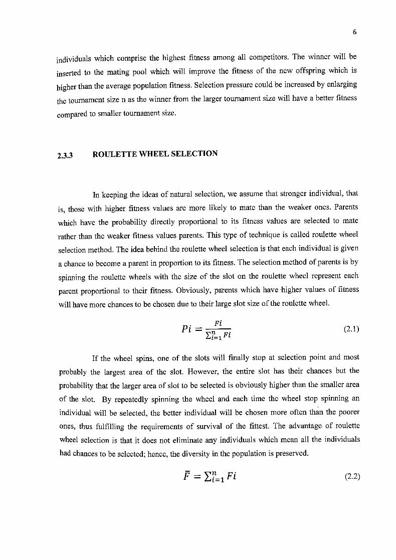
2.3.3 ROULETTE WHEEL SELECTION

In keeping the ideas of natural selection, we assume that stronger individual, that

is, those with higher fitness values are more likely to mate than the weaker ones. Parents

which have the probability directly proportional to its fitness values are selected to mate

rather than the weaker fitness values parents. This type of technique is called roulette wheel

selection method. The idea behind the roulette wheel selection is that each individual is given

a chance to become a parent in proportion to its fitness. The selection method of parents is by

spinning the roulette wheels with the size of the slot on the roulette wheel represent each

parent proportional to their fitness. Obviously, parents which have -higher values of fitness

will have more chances to be chosen due to their large slot size of the roulette wheel.

= Fi(2.1)

If the wheel spins, one of the slots will finally stop at selection point and most

probably the largest area of the slot. However, the entire slot has their chances but the

probability that the larger area of slot to be selected is obviously higher than the smaller area

of the slot. By repeatedly spinning the wheel and each time the wheel stop spinning an

individual will be selected, the better individual will be chosen more often than the poorer

ones, thus fulfilling the requirements of survival of the fittest. The advantage of roulette

wheel selection is that it does not eliminate any individuals which mean all the individuals

had chances to be selected; hence, the diversity in the population is preserved.

= >.1....1Fi (2.2)

7

This type of selection often used in solving TSP. TSP aims at finding out the

individual with higher fitness. The higher the fitness value of an individual the shorter the

route length and the higher selected probability will be. The lower fitness value of individuals

will have the longest route length which will lower selected probability.

4%1881 is rotate0,

IbF*iKI

®12%\

selectiofl point

38'I.

Fittest individual 'Ss( 7------r\ ." \ has largest share of Weakest individual the roulette wheel has smallest share of -

the roulette wheel

Figure 2.1 Roulette wheel selections

2.4 CROSSOVER

Crossover happens between two chromosomes to produce a new offspring that

has genes from both parents. There are three types of crossover that can happen. The first one

is one point crossover. For this type of crossover only one part of the first parent is copied

and the rest is taken in the same order as in the second part. Another type is a two point

crossover which for this type of crossover two parts of the first parent are copied and the rest

between is taken in the same order as in the second parent. The crossing over will produce

8

offspring. The third type of crossover is cloning crossover. This happens when crossover

does not take place between the chromosomes and will produce exact same copies as their

parents. After selection and crossover the average fitness of the chromosome population

should be improved.

77 mm

I ri

F0_ T-1-11 oIo roi:L

Figure 2.2 Basic crossover

2.4.1 CROSSOVER MECHANISM

[10] Some of the most popular generic permutation-based crossover techniques in

algorithm are Partially Mapped Crossover (PMX), Order Crossover (OX), Linear Order

Crossover (LOX) and Cycle Crossover (CX). In PMX method, two crossover points are

selected at random and PMX proceeds by position wise exchanges. The two crossover points

give a matching selection. It affects cross by position-by-position exchange operations. In this

method parents are mapped to each other, hence we can also call it partially mapped

crossover. The PIvix crossover exploits important similarities in the value and ordering

simultaneously when used with reproductive plan. Order crossover (OX) was proposed by

Darwis (1985). This type of crossover keeping traits to their parents' chromosomes, it also

takes relative order of allele values into account while performing the crossover option. The

OX exploits a property of the path representation, that the order of cities is important. It

constructs an offspring by choosing a sub tour of one parent and preserving the relative order

of the cities of the other parent. LOX is the modified version of order crossover which is

Proposed by Falkenauer and Bouffix. The crossover between chromosomes occurs normally

9

like OX but when sliding the parent values around to fit in the remaining open slots of the

child's chromosomes, they are allowed to slide to the left or right. This will ensure that the

offspring to maintain its relative ordering while preserving the beginning and ending values.

Cycle crossover was proposed by Oliver et al (1987). This type of crossover is trying to

produce offspring in such way that each city and its position come from one of the parents. It

is also a little bit different to PMX and OX. The chromosomes are not spitted to form

segments to swap. We can choose the first elements and the rest of the elements will

randomly select.

PARTIALLY MAPPED CROSSOVER (PMX): proposed by Goldberg and Lingle (1985)

Basic procedure of PMX

Step 1: select two positions along the string uniformly at random. The substrings defined by

the two positions are called mapping section

Step 2: exchange two subsfrings between parents to produce proto-children

Step 3: determine the mapping relationship between two mapping sections

Step 4: legalize offspring with the mapping relationship

1. Select the substring at random

IL!I.[I!1L.!Ii[flU M I 2. Exchange substring between parents

Proto-child 1 1 1 2 7 1 :^8^9

3. Determine mapping relationship

uiuumi

mama,

4. Legalize offspring mapping relationship

2 I 9 I 314 1516 I 7 I 8 I 1

Order Crossover (OX): proposed by Davis (1985)

Step 1: select a substring from a parent at random

Step 2: produce a proto-child by copying the substring into the corresponding position of it

Step 3: delete the cities which are already in the substring from the second parent

Step 4: place the cities into the unfixed positions of proto-child from left to right according to

the order of the sequence to produce an offspring

Select substring at random

Parent 1 2 3r

6 7 8 9

Offspring 7 9 FL:4H 5 J 6 1 1 2 8

10

Parent 2

Deleted

11

Cycle Crossover (CX): proposed by Oliver, Smith and Holland (1987)

Step 1: find the cycle which has defined the corresponding position of cities between parents.

Step 2: copy the cities in the cycle to a child with the corresponding positions of one parent

Step 3: determine the remaining cities from the child by deleting those cities which already in

the cycle from the other parent

Step 4: fulfill the child with the remaining cities

1. Fined the cycle defined by parent

Parent 1 2 3 4 5 6 7 8 9

Parent 5 4 6 9 2 3 7 8 1

Cycle 1 * 5 2 > 4 > 9 1

2. Copy the cities in the cycle to a child

Ivratlra !IMF7II[I!1

3. Determine the cities in the cycle to a child

F ! I

The remaining cities

4. Fulfill the child

Offspring 1 2

2.5 MUTATION

0 MW

6I453I7I8I9

12

Mutation represents a change in the gene. It may lead to significant improvement

in fitness of the chromosomes. Holland introduced mutation as a background operator (1975).

Its role is to provide a guarantee that the search algorithm is not trapped in a local optimum.

A new offspring can be achieved by different ways either by flipping, inserting, swapping or

sliding the allele values at two randomly chosen gene positions.

11 -1 0 o o 101110111

Ez^^ [K^ [oh 1 0 0

cI nw 101111111

Figure 2.3 basic mutation