generic branch-cut-and-price - zib · generic branch-cut-and-price ... 5.2 branching on variables...
TRANSCRIPT
Generic Branch-Cut-and-Price
Diplomarbeitbei PD Dr. M. Lubbecke
vorgelegt von Gerald Gamrath 1
Fachbereich Mathematik derTechnischen Universitat Berlin
Berlin, 16. Marz 2010
1Konrad-Zuse-Zentrum fur Informationstechnik Berlin, [email protected]

2
Contents
Acknowledgments iii
1 Introduction 11.1 Definitions . . . . . . . . . . . . . . . . . . . . . . . . . . . . . 31.2 A Brief History of Branch-and-Price . . . . . . . . . . . . . . 6
2 Dantzig-Wolfe Decomposition for MIPs 92.1 The Convexification Approach . . . . . . . . . . . . . . . . . 112.2 The Discretization Approach . . . . . . . . . . . . . . . . . . 132.3 Quality of the Relaxation . . . . . . . . . . . . . . . . . . . . 21
3 Extending SCIP to a Generic Branch-Cut-and-Price Solver 253.1 SCIP—a MIP Solver . . . . . . . . . . . . . . . . . . . . . . . 253.2 GCG—a Generic Branch-Cut-and-Price Solver . . . . . . . . . 273.3 Computational Environment . . . . . . . . . . . . . . . . . . 35
4 Solving the Master Problem 394.1 Basics in Column Generation . . . . . . . . . . . . . . . . . . 39
4.1.1 Reduced Cost Pricing . . . . . . . . . . . . . . . . . . 424.1.2 Farkas Pricing . . . . . . . . . . . . . . . . . . . . . . 434.1.3 Finiteness and Correctness . . . . . . . . . . . . . . . 44
4.2 Solving the Dantzig-Wolfe Master Problem . . . . . . . . . . 454.3 Implementation Details . . . . . . . . . . . . . . . . . . . . . 48
4.3.1 Farkas Pricing . . . . . . . . . . . . . . . . . . . . . . 494.3.2 Reduced Cost Pricing . . . . . . . . . . . . . . . . . . 524.3.3 Making Use of Bounds . . . . . . . . . . . . . . . . . . 54
4.4 Computational Results . . . . . . . . . . . . . . . . . . . . . . 584.4.1 Farkas Pricing . . . . . . . . . . . . . . . . . . . . . . 594.4.2 Reduced Cost Pricing . . . . . . . . . . . . . . . . . . 65
5 Branching 715.1 Branching on Original Variables . . . . . . . . . . . . . . . . . 735.2 Branching on Variables of the Extended Problem . . . . . . . 775.3 Branching on Aggregated Variables . . . . . . . . . . . . . . . 785.4 Ryan and Foster Branching . . . . . . . . . . . . . . . . . . . 79
i
ii Contents
5.5 Other Branching Rules . . . . . . . . . . . . . . . . . . . . . . 825.6 Implementation Details . . . . . . . . . . . . . . . . . . . . . 85
5.6.1 Branching on Original Variables . . . . . . . . . . . . 875.6.2 Ryan and Foster Branching . . . . . . . . . . . . . . . 90
5.7 Computational Results . . . . . . . . . . . . . . . . . . . . . . 915.7.1 Branching on Original Variables . . . . . . . . . . . . 915.7.2 Ryan and Foster Branching . . . . . . . . . . . . . . . 94
6 Separation 996.1 Separation of Cutting Planes in the Original Formulation . . 1006.2 Separation of Cutting Planes in the Extended Problem . . . . 1026.3 Implementation Details . . . . . . . . . . . . . . . . . . . . . 1036.4 Computational Results . . . . . . . . . . . . . . . . . . . . . . 104
7 Results 1097.1 Impact of the Pricing Strategy . . . . . . . . . . . . . . . . . 1107.2 Problem Specific Pricing Solvers . . . . . . . . . . . . . . . . 1177.3 Selected Accelaration Strategies . . . . . . . . . . . . . . . . . 1187.4 Comparison to SCIP . . . . . . . . . . . . . . . . . . . . . . . 120
8 Summary, Conclusions and Outlook 125
A Zusammenfassung (German Summary) 129
B Notation and List of Parameters 131
C Problems 135C.1 The Bin Packing Problem . . . . . . . . . . . . . . . . . . . . 135C.2 The Vertex Coloring Problem . . . . . . . . . . . . . . . . . . 137C.3 The Capacitated p-Median Problem . . . . . . . . . . . . . . 140C.4 A Resource Allocation Problem . . . . . . . . . . . . . . . . . 142
D Tables 147
List of Figures 187
List of Tables 192
Bibliography 200

Acknowledgments
First of all, I want to thank my parents and my brother for their supportand encouragement during my academic studies.
Thanks to Marco E. Lubbecke and Marc E. Pfetsch for leading my studiesinto the direction that is now covered in this thesis. Furthermore, I wish tothank Marco E. Lubbecke for supervising this thesis, for always being avail-able for questions and answering all of them, and for providing me with manyhelpful comments about earlier drafts of this thesis. Additionally, I want tothank Prof. Dr. Martin Grotschel for awakening my interest for combinato-rial optimization and providing the wonderful working athmosphere at ZuseInstitute Berlin.
I wish to thank Timo Berthold, Stefan Heinz, Jens Schulz, Michael Win-kler, and Kati Wolter for reading earlier versions of this thesis, their profes-sional advice and many helpful suggestions. Thanks to Tobias Achterbergfor many hints concerning implementational issues and to Bernd Olthoff foranswering my linguistical questions.
Last but not least, I want to thank my lovely girlfriend Inken Olthoff.She read most of this thesis and provided me with many helpful commentsconcerning content and clarity of presentation. Thanks a lot for your supportand for being there for me whenever I needed it!
iii

iv Chapter 0. Acknowledgments
Chapter 1
Introduction
Many real-world optimization problems can be formulated as mixed inte-ger programs (MIPs). Although solving MIPs is computationally hard [86],state-of-the-art MIP solvers—commercial and non-commercial ones—are ableto solve many of these problems in a reasonable amount of time (see e.g.,Koch [55]). A widely used technique to solve MIPs is the branch-and-cutparadigm which is employed by most MIP solvers.
In this thesis, we regard a different, but related method to solve MIPs,namely the branch-and-price method and its extension, the branch-cut-and-price method. Their success relies on exploiting problem structures in a MIPvia a decomposition. The problem is split into a coordinating problem andone or more typically well structured subproblems that can often be solvedrather efficiently. For many huge and extremely difficult, but well structuredcombinatorial optimization problems, this approach leads to a remarkablybetter performance than a branch-and-cut algorithm.
While there exist very effective generic implementations of branch-and-cut, almost every application of branch-(cut-)and-price is ad hoc, i.e., problemspecific. Therefore, using a branch-(cut-)and-price algorithm usually comesalong with a much higher implementational effort. In recent years, therehas been a development towards the implementation of a generic branch-(cut-)and-price solver. Such a solver should ideally detect the structure of aproblem, perform the decomposition—if promising—and solve the problemwithout further user interaction. An actual implementation of such a fullyautomated solving process is still a long way off. However, there are codesin development, e.g., DIP [78] and BaPCod [93], that just require the user todefine the structure of the problem, before an automated branch-(cut-)and-price solving process is started.
Typically, such a generic implementation does not achieve the perfor-mance of a problem specific one. However, it ideally incorporates sophis-ticated acceleration strategies and other expert knowledge that would bemissing in a basic problem specific implementation and that can partiallycompensate the disadvantage due to the generic approach. A generic imple-mentation provides the possiblity to solve a problem with a branch-(cut-)and-
1

2 Chapter 1. Introduction
price algorithm without any implementational effort and enables researchersto easily test new ideas.
This thesis deals with the generic branch-cut-and-price solver GCG thatextends the existing non-commercial state-of-the-art MIP solver and branch-and-price framework SCIP [3] to a branch-and-price solver. GCG was devel-oped by the author of the thesis and meets the aforementioned demands, i.e.,for a given structure, it performs a decomposition and solves the resultingreformulation with a branch-cut-and-price algorithm. Actually, it still takesinto account the original problem and solves both problems simultaneously,profiting from the additional information.
We present the theoretical background, implementational details, andcomputational results concerning the solver GCG. Computations are carriedout for four classes of problems that are known to fit well into the branch-and-price approach. We investigate whether even a generic approach to branch-cut-and-price is still more effective than a state-of-the-art branch-and-cutMIP solver for these problems.
Outline of the thesis
In the remainder of this chapter we present some basic definitions, give a shortsummary of the history of branch-and-price and review current developmentsconcerning this topic.
The foundation of the generic branch-cut-and-price approach presentedin this thesis is the Dantzig-Wolfe decomposition for MIPs which we discussin Chapter 2.
After that, in Chapter 3 we present the branch-cut-and-price frameworkSCIP which is the basis of our implementation. Furthermore, we describe thegeneral structure of GCG and some general information about the computa-tional experiments that we conducted.
The next three chapters focus on the most important parts of a branch-cut-and-price solver. The solving process of the employed relaxation by col-umn generation is treated in Chapter 4. Chapter 5 describes how this iscombined with a branch-and-bound approach in order to compute an opti-mal solution. Furthermore, in Chapter 6, we describe how to include cuttingplane generation to obtain a branch-cut-and-price algorithm. In each of thesechapters, we first present the theoretical background, followed by implemen-tational details and some computational results.
Chapter 7 deals with the overall performance of the branch-cut-and-pricesolver GCG and the impact of the features mentioned in the previous chapters.Since SCIP with default plugins is a state-of-the-art branch-and-cut basedMIP solver, we also draw a comparison between the results obtained by GCGand SCIP in order to assess the effectiveness of the generic branch-cut-and-price approach.
Finally, we summarize the contents of this thesis in Chapter 8 and presentconcluding remarks as well as directions for further research.

1.1. Definitions 3
In the appendix, we present a German summary, survey the symbolsused in this thesis, define the classes of problems used for our computationalexperiments, and present detailed computational results.
1.1 Definitions
In this section, we define the most important terms that we use in this thesis.For a more detailed introduction into combinatorial optimization, linear andmixed integer programming we refer to [18, 40, 85]. The notation used inthis thesis is summarized in Appendix B.
Problem definitions and some polyhedral theory
For a given set of real-valued variables, a linear program is an optimizationproblem that either minimizes or maximizes a linear objective function, sub-ject to some linear equations or inequalities. Using various transformations,we can transform each linear program into the form that is presented in thefollowing definition.
Definition 1.1 (Linear Program)Let n,m ∈ N, c ∈ Rn, A ∈ Rm×n, and b ∈ Rm. An optimization problem ofthe form
min cTx
s.t. Ax ≥ bx ∈ Rn
+
is called a linear program (LP).
Note that throughout this thesis, we denote by Z+, Q+, and R+ the non-negative integer, rational, and real numbers, respectively.
The set of solutions to an LP forms a polyhedron:
Definition 1.2 (Polyhedron [69])Let n ∈ N.
• A polyhedron P ⊆ Rn is the set of points that satisfy a finite numberm ∈ N of linear inequalities; that is, P = {x ∈ Rn | Ax ≥ b}, where(A, b) is an m× (n+ 1) matrix.
• A polyhedron is said to be rational, if there exists m′ ∈ N and anm′ × (n + 1) matrix (A′, b′) with rational coefficients such that P ={x ∈ Rn | A′x ≤ b′}.
• A polyhedron is called bounded if there exists ω ∈ R+ such thatP ⊆ {x ∈ Rn | − ω ≤ xj ≤ ω for j = 1, . . . , n}. A bounded poly-hedron is called polytope.

4 Chapter 1. Introduction
In this thesis, we restrict ourselves to rational polyhedra and assumerational-valued matrices and vectors. This is actually no limitation in prac-tice since computers are restricted to rational numbers, anyway.
When adding integrality restrictions to a part of the variables of an LP,we get a mixed integer program:Definition 1.3 (Mixed Integer Program)Let n,m ∈ N, c ∈ Qn, A ∈ Qm×n, b ∈ Qm, and I ⊆ [n] := {1, . . . , n}. Anoptimization problem of the form
min cTx
s.t. Ax ≥ bx ∈ Qn
+
xi ∈ Z ∀i ∈ I
(1.1)
is called mixed integer program (MIP).
Like in the case of linear programs, there are several variations of mixedinteger programs like maximization problems and problems containing equal-ity constraints, but all of these can be transformed to the previously statedform, see e.g., [39]. Since each MIP in maximization form can be transferredinto a minimization problem by multiplying the objective function coeffi-cients by minus one, we restricted ourselves to minimization problems in thefollowing. Throughout this thesis, a solution is called integral, if and only ifit satisfies the integrality restrictions, even if continuous variables may havefractional values.
We distinguish the following special cases of MIPs:Definition 1.4A MIP of form (1.1) is called
• an integer program (IP) if I = [n]
• and a binary program (BP) if it is an IP and xi ∈ {0, 1} ∀i ∈ I.
The set X = {x ∈ Qn+ | Ax ≥ b, xi ∈ Z ∀i ∈ I} of solutions to a MIP
is a subset of the polyhedron P = {x ∈ Qn+ | Ax ≥ b}. The latter is the
set of solutions to the so-called LP relaxation of the MIP, i.e., the LP thatwe obtain by discarding the integrality restrictions of the MIP. Due to theintegrality restrictions, the set X is not a polyhedron. However, since weassumed rational data, its convex hull conv(X) is a polyhedron:
Theorem 1.5 ([65])If P is a rational polyhedron and X = P ∩ {x ∈ Qn
+ | xi ∈ Z ∀i ∈ I} 6= ∅,then conv(X) is a rational polyhedron whose extreme points are a subset ofX and whose extreme rays are the extreme rays of P .
This does not neccessarily hold for polyhedra not restricted to rationaldata and since Theorem 1.5 is an important result which we will use inChapter 2, it is one of the reasons for assuming rational data througout thisthesis.

1.1. Definitions 5
Solving methods
There exist solving methods which can solve LPs in polynomial time, e.g.,the ellipsoid method [52, 53] and interior point methods [51, 81]. In practice,the simplex method [21] is often used, although it may have an exponentialrunning time. In the context of MIP solving, however, it performs empiricallybetter than the alternatives mentioned previously. In this thesis, we willtherefore restrict ourselves to the simplex method for solving LPs.
Adding integrality constraints increases the complexity of the problem:MIP-solving is NP-hard [86].
Two methods for solving MIPs are LP based branch-and-bound and thegeneral cutting plane method. Both rely heavily on the LP-relaxation of theproblem, i.e., the linear program obtained when disregarding the integralityrestrictions of the MIP.
The branch-and-bound algorithm, a form of divide-and-conquer, dividesthe problem into subproblems until these can easily be solved to optimality.For each subproblem, the LP-relaxation is solved, providing a lower bound(also called dual bound) on the best feasible solution of the current subprob-lem. On the other hand, the best known primal solution to the global problemis referred to as the incumbent, its objective value is called upper bound orprimal bound. If the lower bound of a subproblem is greater or equal to theupper bound, the current subproblem can be ignored since it cannot contain asolution with objective value better than that of the incumbent. Otherwise,the current problem is divided into multiple—typically two—subproblems.These two steps are called bounding and branching, respectively, which givesrise to the name of the algorithm. They are repeated until all subproblemsare either solved to optimality or discarded due to their lower bound.
The branch-and-bound procedure can easily be illustrated as a tree, whereeach node represents one of the (sub-)problems. In particular, the root nodeof the tree represents the initial problem. Whenever a problem is divided intosubproblems, these problems are represented by child nodes of the currentproblem’s node in the tree. When a subproblem can be ignored due to thebounding process, the corresponding node is pruned.
On the other hand, in the general cutting plane method, the LP relaxationof the problem is also solved first. If the computed optimal LP solutionis fractional, a valid inequality is added to the LP, which is satisfied byall feasible solutions of the MIP, but violated by the current fractional LPsolution. Thus we can say that this inequality “cuts off” the fractional LPsolution, it is therefore called cutting plane. Since geometrically, the cut canbe seen as a hyperplane that separates the vector corresponding to the LPsolution from all feasible solutions of the MIP, this process is also referred toas separation. This is repeated, until the optimal LP solution is integral andtherefore an optimal solution of the MIP.
Most state-of-the-art MIP solvers use a combination of these two methods,called branch-and-cut. The LP relaxation of the subproblems is strengthened

6 Chapter 1. Introduction
by a reasonable number of cutting planes thereby trying to preserve its nu-merical stability. Often, only the LP relaxation of the root-node is strength-ened by cutting planes, afterwards, the problem is solved by a branch-and-bound method.
Furthermore, branch-and-price [10] is a variant of branch-and-bound,where only a subset of the variables is given explicitly, most of them arehandled implicitly. The key idea is that most of the variables will neverbe part of an optimal LP solution. They would just slow down the solu-tion process and would consume too much memory. During the optimizationprocess, at each node, the LP relaxation is solved with a column generationapproach: Whenever one of the implicitly given variables might improve thecurrent LP solution, it is added explicitly to the problem. We go into detailabout column generation and branching in this context in Chapters 4 and 5,respectively.
Finally, branch-cut-and-price is a combination of branch-and-price andbranch-and-cut. The variables are given implicitly and added to the problemonly when needed. Additionally, cutting planes are added to the problemduring the solving process in order to strenghen the LP relaxation. Variablesand cutting planes are created alternately. Cutting plane generation in thiscontext will be treated in Chapter 6.
1.2 A Brief History of Branch-and-Price
When talking about the history of branch-and-price, we have to start withcolumn generation which is the foundation of branch-and-price.
Column generation is a method to solve linear problems with a huge num-ber of variables. Instead of solving the complete linear program, we solve arestricted problem containing only a subset of the variables; remaining vari-ables are treated implicitly. Therefor, a high number of smaller, typically wellstructured subproblems—called pricing problems—are solved that determinesome of the implicitly given variables which are then explictly added to therestricted problem in order to improve its solution. Due to their structure,the pricing problems can typically be solved rather efficiently. We give adetailed description of column generation in Section 4.1.
Column generation has its roots in the 1960s when George B. Dantzig andPhilip Wolfe proposed their decomposition principle for linear programs [22,23]. The original problem is reformulated as a linear problem with (typically)an exponential number of variables. These variables represent the extremepoints and rays of the polyhedra corresponding to the pricing problems whichare linear subproblems.
Shortly after that, Paul C. Gilmore and Ralph E. Gomory presented aformulation of an integer program—the cutting stock problem—containing ahuge number of variables that were implicitly treated [36, 37]. The pricingproblem was a knapsack problem. However, only linear programming meth-

1.2. A Brief History of Branch-and-Price 7
ods were used to solve the problem, so integrality of the variables could notbe enforced: “That integers should result of the example is, of course, for-tuitous” [36]. Nevertheless, similar reformulations were proposed for severalother combinatorial optimization problems [66].
Combining the column generation approach with a branch-and-boundalgorithm in order to solve these problems to integrality poses several chal-lenges [8, 47] which we will discuss in Chapters 4 and 5. Hence, several yearshad to go by before column generation was successfully combined in practicewith branch-and-bound to a method called branch-and-price or IP columngeneration.
In the 1990s, this concept was applied for example to the bin packingproblem [90], the vertex coloring problem [63], and the generalized assignmentproblem [83]; problem independent surveys are given in [10, 97]. Besides,the column generation approach was based on a decomposition for integerprograms [28, 91] that is similar to the Dantzig-Wolfe decomposition. Thisdecomposition principle is presented in Chapter 2 of this thesis.
In the last decade, several general acceleration strategies for the branch-and-price process were proposed [26, 57] and branch-and-price was success-fully applied to many problems [27]. Furthermore, branch-and-price was com-bined with the general cutting plane method to branch-cut-and-price [33, 87].We will go into detail about this in Chapter 6.
Nowadays, branch-and-price is a well-established method to solve hugeand extremely difficult combinatorial optimization problems. Its success re-lies on exploiting structures contained in the problem via a decompositionand being able to solve the occuring pricing problems rather efficiently withproblem specific algorithms.
The most widely used method to solve MIPs, however, is the branch-and-cut algorithm employed by most state-of-the-art MIP solvers. Although theuser can extend the existing branch-and-cut solvers by adding problem spe-cific plugins, these solvers—commercial and non-commercial ones—featurevery effective generic algorithms that can be used to solve many generalMIPs without further problem knowledge.
The situation differs strongly for branch-and-price algorithms. Thereexist several branch-cut-and-price frameworks like ABACUS [48], BCP [80],MINTO [68], and SCIP [3]—which is the one we used and extended in thisthesis. However, one cannot simply read in a problem and just solve itwith a branch-and-price algorithm since the most important properties—likethe pricing routine and a branching scheme—have to be implemented andprovided by the user. Therefore, even when using the aforementioned possi-bilities, several problem specific parts of the solver have to be implementedbefore a problem can be solved.
It would be much more satisfactory to have generic implementations alsofor branch-and-price. These implementations shoul provide the essentialfunctionalities to solve a general—or just a well structured—MIP with abranch-and-price approach. This could be used to easily test new ideas. Fur-

8 Chapter 1. Introduction
thermore, if it turns out that the branch-and-price approach performs wellfor specific problems, some of the generic functionalities could be replacedby problem specific ones to speed up the solving process.
In recent years, there has been some progress into this direction. FrancoisVanderbeck has been developing important features [92, 94, 96, 95] for its ownimplementation called BaPCod which is “a prototype code that solves MixedInteger Programs (MIP) by application of a Dantzig-Wolfe reformulationtechnique” [93].
Also the COIN-OR initiative [20] hosts a generic decomposition code,called DIP [76, 77] (formerly known as DECOMP), which is a “framework forimplementing decomposition-based bounding algorithms for use in solvinglarge-scale discrete optimization problems” [78].
The constraint programming G12 project develops “user-controlled map-pings from a high-level model to different solving methods” [75], one of whichis branch-and-price.
Among these projects, only DIP is currently (March 2010) open to thepublic, but just as a trunk development version, there has not been a release,yet.
For all these implementations, the user has to specify the structure ofa problem after reading it in and an automated Dantzig-Wolfe decomposi-tion is performed that reformulates the problem. The reformulation is thensolved with a branch-and-price algorithm; solving the pricing problems andbranching are handled in a generic way.
In relation to this thesis, we developed our own implementation of abranch-cut-and-price solver called GCG. It extends the branch-cut-and-priceframework SCIP [3], which already features one of the fastest non-commercialMIP solvers, to a branch-cut-and-price solver.

Chapter 2
Dantzig-Wolfe Decompositionfor MIPs
The Dantzig-Wolfe decomposition for linear programs [22, 23] can be trans-ferred to MIPs in two different ways: the convexification approach [28, 91]and the discretization approach [91, 47]. The former is the more general one,while the latter leads to better computational results when the problem hasthe appropriate structure so that it can be applied. The symbols related tothe decomposition that are introduced in this chapter can also be looked upin Appendix B.
In this chapter, we present both concepts and and a comparison of them.Our presentation is based on [29, 57] for the convexification approach and [92,96] for the discretization approach.
The first steps of the decomposition are the same in both approaches.Suppose we are given a MIP of the following form, which we will call theoriginal formulation:
Model 2.1 (Original Program)
z?OP = min
∑k∈[K]
ckTxk
s.t.∑
k∈[K]
Akxk ≥ b (2.1)
Dkxk ≥ dk ∀k ∈ [K] (2.2)
xk ≥ 0 ∀k ∈ [K] (2.3)
xki ∈ Z ∀k ∈ [K], i ∈ [n?
k]. (2.4)
The problem is modeled using K ∈ N vectors of variables xk ∈ Qnk , k ∈[K] and corresponding objective function vectors ck ∈ Qnk . We have twotypes of restrictions, linking constraints and structural constraints.
9

10 Chapter 2. Dantzig-Wolfe Decomposition for MIPs
A1 A2 · · · AK
D1
D2
. . .
DK
×
x1
x2
...
xK
≤
b
d1
d2
...
dK
Figure 2.1: Structure of the constraints in the original problem
The linking constraints (2.1) are given by coefficient matricesAk ∈ QmA×nk and a right-hand side b ∈ QmA and are “global” constraintsthat contain variables of different vectors xk.
The structural constraints (2.2) can be divided into K blocks, where eachblock k ∈ [K] imposes some restrictions on the variable vector xk. Theseconstraints are given by matrices Dk ∈ Qmk×nk and right-hand sides dk ∈Qmk .
In addition to that, all variables are non-negative and for each variablevector xk, the first n?
k variables are of integral type.The structure of the contraint maxtrix of the original formulation is il-
lustrated in Figure 2.1. This structure will be called bordered block diagonalin the following.
Typically, when using the Dantzig-Wolfe reformulation, we have multipleblocks, i.e., k > 1 . However, if we have just one block but the structuralconstraints define a combinatorial optimization problem that can be solvedmuch more efficiently than the global problem, the Dantzig-Wolfe reformu-lation can be used to exploit this structure, too. In this case, the linkingconstraints do not link the values of the variables of different blocks but arecomplicating constraints that destroy the structure of the subproblem whentreating all constraints together.
We will now introduce a set Xk for each block k ∈ [K] that contains thevectors satisfying the structural constraints as well as the non-negativity andintegrality constraints associated with this block:
Xk := {xk ∈ Zn?k
+ ×Qnk−n?k
+ | Dkxk ≥ dk}. (2.5)
Restricting the values of xk to this set Xk for all k ∈ [K], we treat con-straints (2.2), (2.3) and (2.4) implicitly and can therefore omit them in thecompact formulation:

2.1. The Convexification Approach 11
Model 2.2 (Compact Program)
z?CP = min
∑k∈[K]
ckTxk
s.t.∑
k∈[K]
Akxk ≥ b (2.6)
xk ∈ Xk ∀k ∈ [K]. (2.7)
At this point, the further steps differ for the convexification approachand the discretization approach. We start with a detailed description of theconvexification approach. After that, we present the discretization approachand give a comparison between both approaches.
2.1 The Convexification Approach
In the convexification approach, we will now represent each vector xk ∈ Xk
by a convex combination of extreme points plus a conical combination ofextreme rays, like it is also done in the Dantzig-Wolfe decomposition forlinear programs (see [22, 23]).
In contrast to the classical Dantzig-Wolfe decomposition, the set Xk is nota polyhedron since we have integrality conditions on some of the variables.It is, however, the set of solutions to a MIP defined by rational data, soits convex hull is a polyhedron (see Section 1.1). From now on, we thusinvestigate the convex hull of Xk in order to get a polyhedron that we candescribe by a finite number of extreme points and extreme rays:
Theorem 2.3 (Minkowski and Weyl Theorems)A set X ⊆ Qn is a polyhedron if and only if there exist finite setsP = {p1, p2, . . . , pm} ⊆ Qn and R = {r1, r2, . . . , r`} ⊆ Qn such thatX = conv(P ) + cone(R).
So, for each set Xk there exist finite sets Pk ⊆ Zn?k
+ ×Qnk−n?k
+ of extreme
points of conv(Xk) and Rk ⊆ Zn?k
+ × Qnk−n?k
+ of extreme rays of conv(Xk) sothat each xk ∈ Xk ⊆ conv(Xk) can be represented as a convex combinationof the extreme points plus a non-negative combination of the extreme rays,i.e., for each xk ∈ Xk there exists λ ∈ Q|P |+|R|+ with
xk =∑p∈P
λp · p+∑r∈R
λr · r;∑p∈P
λp = 1. (2.8)
With this result, we can substitute xk in the compact formulation (2.2)according to (2.8) and get the following extended fomulation.
For ease of presentation, we define
ckq := ckT q and ak
q := Akq for q ∈ Pk ∪Rk, for all k ∈ [K]. (2.9)

12 Chapter 2. Dantzig-Wolfe Decomposition for MIPs
Model 2.4 (Extended Formulation for Convexification)
z?EPC = min
∑k∈[K]
∑p∈Pk
cpλkp +
∑k∈[K]
∑r∈Rk
crλkr
s.t.∑
k∈[K]
∑p∈Pk
apλkp +
∑k∈[K]
∑r∈Rk
arλkr ≥ b (2.10)
∑p∈Pk
λkp = 1 ∀k ∈ [K] (2.11)
λk ≥ 0 ∀k ∈ [K] (2.12)∑p∈Pk
pλkp +
∑r∈Rk
rλkr = xk ∀k ∈ [K] (2.13)
xki ∈ Z. ∀k ∈ [K],
i ∈ [n?k]. (2.14)
This problem is a reformulation of the compact problem and thus equiv-alent to the original problem. In addition to the K variable vectors xk thatrepresent the solution vectors of the compact problem (Model 2.2), we getfor each block k ∈ [K] one variable λk
p for each extreme point p ∈ Pk as wellas one variable λk
r for each extreme ray r ∈ Rk.
For each k ∈ [K], the coupling constraints (2.13) link the variable xk tothe values given by the selected combination of extreme points and extremerays of conv(Xk), which is a convex one for the former and a conical onefor the latter because of constraints (2.11) and (2.12). Using Theorem 2.3(Minkowsky and Weyl), it follows xk ∈ conv(Xk) and, due to the integralityconstraints (2.14), even xk ∈ Xk. Therefore, for each k ∈ [K], xk satisfiesthe corresponding constraint of type (2.7) in the compact problem.
The objective function and constraints (2.10) are equivalent to their coun-terparts in the compact formulation: xk was substituted according to (2.8)and definition (2.9) was used.
When we want to solve the LP-relaxation of Model 2.4, we relax the in-tegrality of the variables xk and remove constraints (2.14). As the vectorsxk are only used to enforce integrality, after removing the integrality con-straints (2.14), we can also remove the coupling constraints (2.13) as well asthe variable vectors xk, k ∈ [K], from the relaxation and get the followinglinear program as a relaxation of Model 2.4.
2.2. The Discretization Approach 13
Model 2.5 (Master Problem for Convexification)
z?MPC = min
∑k∈[K]
∑p∈Pk
cpλkp +
∑k∈[K]
∑r∈Rk
crλkr
s.t.∑
k∈[K]
∑p∈Pk
apλkp +
∑k∈[K]
∑r∈Rk
arλkr ≥ b (2.15)
∑p∈Pk
λkp = 1 ∀k ∈ [K] (2.16)
λk ≥ 0 ∀k ∈ [K] (2.17)
This master problem (MP) is a relaxation of the extended formulationand therefore, its optimal solution value is also a lower bound for the op-timal solution value of the original problem. Each optimal solution to themaster problem (Model 2.5) can be transformed into a (possibly fractional)solution candidate of the original problem. As we will in Section 2.3, themaster problem typically gives rise to a better lower bound than the LP-relaxation of the original problem, but it also has a big handicap: It has,in general, exponential many variables and these variables are given implic-itly. Computing even just one of the variables is in general NP-hard as theycorrespond to solutions of an arbitrary MIP. Hence, computing all extremepoints and extreme rays in advance is far to costly and even if we would do so,an LP containing all the variables explicitly would consume a vast amount ofmemory and would be computationally hard to solve. In Chapter 4, we willdescribe how to solve this master problem in a more efficient way by usingcolumn generation.
2.2 The Discretization Approach
In many cases when a problem can be decomposed in the described way, allthe blocks or a part of them are identical, i.e., the polyhedra conv(Xk) areidentical and all contained points have the same objective function value. Inthe bin packing problem (see Section C.1), for example, all bins have thesame size, so all the blocks are identical.
In the convexification approach however, in order to force the integralityof the points chosen in each polyhedron, we have to distinguish between theextreme points related to different blocks even if the polyhedra of these blocksare identical. Therefore, we need to create multiple variables for the sameextreme point, each of which is related to a different block.
In case of pure integer programs, we can use the discretization approachto avoid this.
Starting with the original program (Model 2.1), we transform it to thecompact program (Model 2.2) like described previously. Instead of using theMinkowski and Weyl theorems to get a representation of all points x ∈ Xk

14 Chapter 2. Dantzig-Wolfe Decomposition for MIPs
and introducing variables for the extreme points and extreme rays, we simplycreate integral variables λk
p and λkr for a number of points p ∈ Xk and rays
r ∈ Zn. Again, we only allow a convex combination of points what is equalto choosing exactly one of them this time.
The following therorem, a slightly modified version of Theorem 6.1 in [69],shows that it is possible to get such a representation with finitely many pointsand rays for each set Xk defined like in (2.5).
Theorem 2.6If P = {x ∈ Qn
+ | Ax ≤ b} 6= ∅ and S = P ∩ Zn, where (A, b) is a rationalm× (n+ 1) matrix, then there exist a finite set of points {q`}`∈L of S and afinite set of rays {rj}j∈J of P such that
S =
x ∈ Qn+ | x =
∑`∈L
α`q` +
∑j∈J
βjrj ,∑`inL
α` = 1, α ∈ Z|L|+ , β ∈ Z|J |+
.
For the proof of this theorem, we refer to [69]. An integer matrix isrequired there, but we can easily scale the rational matrix (A, b) to integervalues without changing the problem.
Corollary 2.7For each set Xk defined like in (2.5), there exist finite sets Pk ⊆ Xk andRk ⊆ Znk such that the following is equivalent:
1. x ∈ Xk
2. There exists λ ∈ Z|Pk|+|Rk|+ with
∑p∈Pk
λp = 1 such that
x =∑p∈Pk
λpp+∑r∈Rk
λrr. (2.18)
This looks similar to the Minkowski and Weyl theorems 2.3, except thatthe factors λ are integral. This is compensated by a higher number of pointsin the set Pk while the number of rays stays the same.
Using this representation of all points in Xk, we can substitute xk in thecompact formulation (model 2.2) and get an extended formulation for thediscretization approach using the abbreviations (2.9).

2.2. The Discretization Approach 15
Figure 2.2: The points represented by variables in the convexification (left)and the discretization approach (right) for a bounded polyhedron conv(Xk)
Model 2.8 (Extended Formulation for Discretization)
z?EPD = min
∑k∈[K]
∑p∈Pk
ckpλkp +
∑k∈[K]
∑r∈Rk
ckrλkr
s.t.∑
k∈[K]
∑p∈Pk
akpλ
kp +
∑k∈[K]
∑r∈Rk
akrλ
kr ≥ b (2.19)
∑p∈Pk
λkp = 1 ∀k ∈ [K]
(2.20)
λk ∈ Z|Pk|+|Rk|+ ∀k ∈ [K]
(2.21)
Model 2.8 is again a reformulation of the compact problem and thus alsoof the original problem. As mentioned previously, xk is replaced accordingto (2.18) and (2.9) in objective function and linking constraints. Due toTheorem 2.6, constraints (2.20) and (2.21) are equivalent to constraints (2.7)in the compact formulation.
Hence, we can impose integrality constraints directly on the variablesrelated to the points and rays in order to enforce integrality of the corre-sponding solution in the original program and do not need the vectors xk
anymore.Apart from the missing variable vectors xk and the integrality of the λ
variables, this looks similar to the extended formulation of the convexificationapproach. The only further difference is given implicitly in the definition ofthe sets Pk and Rk.
The relation between the sets of variables in the convexification and thediscretization approach are pictured in Figure 2.2 and Figure 2.3. The poly-hedron conv(Xk) is colored grey while the points and rays contained in thesets Pk and Rk, respectively, are colored red. The chosen points in the dis-cretization approach for an unbounded polyhedron are the smallest set of theform given in Corrolary 2.7, one could also choose a bigger set.

16 Chapter 2. Dantzig-Wolfe Decomposition for MIPs
Figure 2.3: The points and rays represented by variables in the convexifica-tion (left) and the discretization approach (right) for an unbounded polyhe-dron conv(Xk)
Furthermore, when relaxing the integrality restrictions, we get a masterproblem, that is also equivalent to the master problem in the convexificationapproach.
Model 2.9 (Master Problem for Discretization)
z?MPD = min
∑k∈[K]
∑p∈Pk
ckpλkp +
∑k∈[K]
∑r∈Rk
ckrλkr
s.t.∑
k∈[K]
∑p∈Pk
akpλ
kp +
∑k∈[K]
∑r∈Rk
akrλ
kr ≥ b (2.22)
∑p∈Pk
λkp = 1 ∀k ∈ [K] (2.23)
λk ≥ 0 ∀k ∈ [K] (2.24)
The constraints (2.23) and (2.24) assure that a convex combination ofpoints and a conical combination of rays is chosen. The rays Rk have thesame directions as in the convexification approach, they are only scaled tointegral values. The set of points Pk contains all the extreme points that arecontained in the convexification approach, but even some more points. Theseadditional points, however, are all interior points, so they do not changethe polyhedron described by conv(Pk) + cone(Rk). Thus, this polyhedronis the same for the two different definitions of the sets Pk and Rk in theconvexification and the discretization approach: it is the set conv(Xk), theconvex hull of the set Xk.
Therefore, in both master formulations, we optimize over the same poly-hedron, namely the intersection of the polyhedron defined by the linkingconstraints and the polyhedron conv(Xk) and both problems have the sameobjective function, so these problems are equivalent.
The integrality restrictions on the λ-variables in the extended formula-tion 2.8 allow standard primal heuristics to find feasible solutions and also

2.2. The Discretization Approach 17
cutting planes could be derived from this formulation. The biggest advantage,however, is that we do not need the relation between blocks and variables inorder to enforce integrality, so we can treat identical blocks jointly and needto create the same point only once for all these blocks.
Suppose [K] can be partitioned into L sets K`, ` ∈ [L] of identical blocks,called identity classes in the following. For ease of presentation, we assumethat the first L blocks are pairwise different and for 1 ≤ ` ≤ L, block `represents the set K`, i.e.,
K` = {k ∈ [K] | ck = c`, Ak = A`, Dk = D`, dk = d`}.
Since all blocks k ∈ K` are identical, they have the same set of solutionsXk = X` and thus also the same points Pk = P` and rays Rk = R` in therepresentation.
Moreover, in the extended formulation 2.8, there is no distinction be-tween two variables of different, identical blocks representing the same point(or ray), they have the same objective function coefficient and the same co-efficients in the linking constraints (2.19). Therefore, we can aggregate thevariables representing the same point or the same ray and get new variables
λ`p =
∑k∈K`
λkp (2.25)
and
λ`r =
∑k∈K`
λkr . (2.26)
This leads to the following aggregated extended formulation, again usingthe abbreviations (2.9).
Model 2.10 (Aggregated Extended Formulation for Discretization)
z?EPDa = min
∑`∈[L]
∑p∈P`
clpλ`p +
∑`∈[L]
∑r∈R`
clrλ`r
s.t.∑`∈[L]
∑p∈P`
alpλ
`p +
∑`∈[L]
∑r∈R`
alrλ
`r ≥ b (2.27)
∑p∈P`
λ`p = |K`| ∀` ∈ [L] (2.28)
λ` ∈ Z|P`|+|R`|+ ∀` ∈ [L] (2.29)
In the objective function and in the linking constraints (2.19), we intro-duced the variables λ`
p and λ`r according to their definitions (2.25) and (2.26)
and we now get one summand for each class ` ∈ [L] of identical blocks insteadof one for each block k ∈ [K].

18 Chapter 2. Dantzig-Wolfe Decomposition for MIPs
The convexity constraints (2.20) of identical blocks are added up, wesubstitute λ`
p =∑
k∈K`λk
p, and the right-hand side changes to the cardinalityof the class of identical blocks.
Finally, the integrality constraints (2.21) of identical blocks are combinedto constraints (2.29) forcing the aggregated variables λ` to be integral.
Altogether, this leads to the following lemma:
Lemma 2.11 (Equivalence of the Extended Formulations)The aggregated extended problems (Model 2.10) is equivalent to the extendedproblem for the discretization apporach (Model 2.8): Each solution toModel 2.8 corresponds to a solution to Model 2.10 with the same objectivefunction value and vice versa.
Proof 2.12Given a solution to Model 2.8, by applying the aggregation prescriptions (2.25)and (2.26) we get values of the aggregated variables that form a feasible so-lution for Model 2.10 with the same objective value.
On the other hand, if we have a solution λ to Model 2.10, for each class ofidentical blocks, all variables have non-negative integer values and the valuesof variables that belong to points sum up to |K`|. We can distribute thesevalues among the set K` of identical blocks of this class to get a feasiblesolution of Model 2.8 by doing the following for each class ` ∈ [L] of identicalblocks. Let λ`
p1, . . . , λ`
psbe the variables corresponding to points that have
strictly positve value in the given solution and K` = {k1, . . . , k|K`|}. We set
λk1r = λ`
r ∀r ∈ R`
λkr = 0 ∀k ∈ K` \ {k1}, r ∈ R`.
For i = 1, . . . , s and j =∑i−1
t=1 λ`pt
+ 1, . . . ,∑i
t=1 λ`pt
, we set:
λkjpi = 1
λkjp = 0 ∀p ∈ P` \ {pi}.
That is, we distribute the solution values among the set K` of identical blocksof this class, such that in each block, exactly one variable corresponding to apoint gets value 1, all other variables receive value 0.
Hence, the convexity constraints of Model 2.8 are satisfied, as well asconstraints (2.19), since the value of each variable in the given solution wasdistributed among variables that have the same coefficients in (2.19) as thegiven variable in (2.27). Finally, the values were also distributed among vari-ables with the same objective function coefficient, thus, the objective functionvalue stays the same. 2
2.2. The Discretization Approach 19
The disaggregation of a solution to the aggregated extended problempresented in Proof 2.12 is not unique. By permuting the set of blocks corre-sponding to an identity class, we get a different solution in the non-aggregatedextended problem and in the original problem. This is due to the afore-mentioned symmetry: In the original and in the non-aggregated extendedproblem, we get, for each feasible solution, equivalent solutions by permutingidentical blocks. All these solutions correspond to a single solution in the ag-gregated extended problem, since we do not distinguish the identical blocksin this model.
Corollary 2.13The following problems are equivalent:
• the original problem (Model 2.1)
• the compact problem (Model 2.2)
• the extended problem for the convexification approach (Model 2.4)
• the extended problem for the discretization approach (Model 2.8)
• the aggregated extended problem for the discretization approach(Model 2.10)
When relaxing the integrality of the λ` variables in order to get the LPrelaxation, we get a master problem quite similar to the master problem inthe convexification approach (Model 2.5).
Model 2.14 (Aggregated Master Problem for Discretization)
z?MPDa = min
∑`∈[L]
∑p∈P`
clpλ`p +
∑`∈[L]
∑r∈R`
clrλ`r
s.t.∑`∈[L]
∑p∈P`
alpλ
`p +
∑`∈[L]
∑r∈R`
alrλ
`r ≥ b∑
p∈P`
λ`p = |K`| ∀` ∈ [L]
λ` ≥ 0 ∀` ∈ [L]
Like the extended formulations, the master problems of the two differentapproaches are equivalent, as the following lemma states.
Lemma 2.15 (Equivalence of the Master Problems)The aggregated master problem for the discretization approach (Model 2.14) isequivalent to the master problem for the convexification approach (Model 2.5):Each solution to one of the problems corresponds to a solution of the otherproblem with the same objective function value and vice versa.

20 Chapter 2. Dantzig-Wolfe Decomposition for MIPs
Proof 2.16The convexification master problem (Model 2.5) is equivalent to the non-aggregated master problem of the discretization approach (Model 2.9), so itis sufficient to show that the aggregated master problem for the discretizationapproach (Model 2.14) is equivalent to Model 2.9.
Given a solution to Model 2.9, by applying the aggregation prescriptions(2.25) and (2.26), we get values of the aggregated variables that form a feasiblesolution for Model 2.14 with the same objective value.
On the other hand, if we have a solution λ to Model 2.14, for each classof identical blocks, all variables have non-negative values and the values ofvariables that belong to points sum up to |K`|. We construct a solution λ toModel 2.9 in the following way: For each class of identical blocks ` ∈ [L] weset
λkq =
λ`q
|K`|∀k ∈ K`, q ∈ P` ∪R`.
The values are distributed among variables with the same coefficients in ob-jective function and linking constraints, so the objective function value staysthe same and constraints (2.22) are still satisfied. The non-negativity con-straints (2.24) are still satisfied, too, and by dividing the values by |K`|, thesum of values of variables corresponding to points is 1 for each block, so con-straints (2.23) are also satisfied. Hence, this solution is feasible for Model 2.9and has the same objective value as the given one. 2
Thus, the aggregated master problem for discretization (Model 2.14)has the same optimal objective value as the convexification master prob-lem (Model 2.5) and the discretization master problem (Model 2.9), i.e.,z?MPC = z?
MPD = z?MPDa . In the following, when speaking of one of these
master problems, we will simply denote its optimal objective value by z?MP .
Remark 2.17When transferring a solution of the aggregated master problem (Model 2.14)into a solution to the original problem, we also need to distribute the valuesof variables corresponding to a class of identical blocks to the single blocks ofthis class. This could be done in the way as described in Proof 2.16, but inpractice, it is much more efficient to preserve integrality of the variables. Asfar as possible, in each block, exactly one point should be chosen, only for thelast blocks, when all remaining values are fractional, a convex combinationof multiple points has to be chosen.
This way, an integral solution of the aggregated master problem results inan integral solution of the original problem after the transformation. For amore sophisticated scheme to transfer a solution from the aggregated extendedproblem to the original problem which makes use of a lexicographical orderwe refer to [95].
Like the convexification master problem, the both master problems for thediscretization approach have in general an exponential number of variables.

2.3. Quality of the Relaxation 21
We will give a detailed description of how to solve them with a columngeneration approach in Chapter 4.
Let us regard again the variables corresponding to integral points. Likementioned previously, we do not need them to solve the master problem andas we will see later, we will only create variables corresponding to extremepoints in the column generation procedure. Nevertheless, in order to findoptimal or even feasible solutions to one of the extended formulations forthe discretization approach (Model 2.8 or Model 2.10), interior points areessential since they may be contained in an optimal solution or the linkingconstraints may even forbid solutions containing only extreme points.
It is important to notice, that for a pure BP, all feasible integral pointsare extreme points, so in this case, we do not need to bother about creatinginterior points in the column generation procedure.
For an IP, we have two different possibilities: On the one hand, if the IPis bounded, it can be converted into a BP by replacing each integral variableby some binary variables. On the other hand, we can use branching rulesthat modify the subproblems, the set of solutions Xk, k ∈ [K] and thus alsothe polyhedra conv(Xk), so that each initially interior point will become anextreme point at some level in the branching tree. In Chapter 5, we willdiscuss different branching rules with that property.
The discretization approach can also be applied to MIPs but this is morecomplicated. We will only give a short overview at this point, for which weassume that the MIP is bounded. For a deeper discussion, we refer to [96].Since the MIP is bounded, the projection of conv(Xk) to the integral vari-ables leads to a set Pk of integral points and for each point of this set, we geta polytope in the continuous variables. Like in the discretization approachfor IPs, we choose exactly one point of the set Pk and for the continuousvariables, we choose a convex combination of extreme points of the poly-tope corresponding to that integral point. The number of variables is stillfinite since we have a finite number of integral points and for each of thesepoints a finite number of extreme points of the corresponding polytope in thecontinuous variables.
2.3 Quality of the Relaxation
If we would solve the original problem (Model 2.1) with a standard branch-and-bound algorithm, we would get a lower bound z?
LP on the optimal ob-jective value z?
OP by solving its LP-relaxation.The LP relaxation of the extended formulation is the master problem,
Model 2.5 for the convexification, Model 2.9 or 2.14 for the discretizationapproach. All these three models give rise to the same lower bound z?
MP
which is in general a better bound than the bound z?LP obtained by solving
the LP relaxation of the original problem:

22 Chapter 2. Dantzig-Wolfe Decomposition for MIPs
Theorem 2.18For the optimal objective value z?
OP to the original problem and the solutionsz?LP and z?
MP of its LP relaxation and the master problem, respectively, thefollowing holds:
z?LP ≤ z?
MP ≤ z?OP . (2.30)
Proof 2.19In the LP relaxation, we minimize over the intersection of the two polyhedra
PA =
(x1T, . . . , xKT
)T ∈ Qn+ |
∑k∈[K]
Akxk ≥ b
and
PLPD =
{(x1T
, . . . , xKT)T ∈ Qn
+ | Dkxk ≥ dk ∀k ∈ [K]}
.
The set of feasible solutions to the master problem is the intersection of PA
with the polyhedron
PMPD = conv(X1)× · · · × conv(XK)
that further restricts the polyhedron PLPD since it is the inclusion minimal
polyhedron containing all points that satisfy both Dkxk ≥ dk as well as theintegrality restictions for each block.
Therefore, PMPD ⊆ PLP
D and so PA ∩ PMPD ⊆ PA ∩ PLP
D . It follows
z?LP = min
x∈PA∩P LPD
{(cT1 , . . . , c
TK)x
}≤ min
x∈PA∩P MD
{(cT1 , . . . , c
TK)x
}= z?
MP
and since the master problem is a relaxation of the extended formulationwhich is equivalent to the original problem, it follows (2.30). 2
It can be shown (see [35]) that the master problem is the dual formulationof the Lagrangean dual obtained by dualizing the linking constraints (2.1),so the master problem provides the same lower bound as the Lagrangeanrelaxation.
The bound obtained by the master problem is typically strictly betterthan the LP bound, using it as a relaxation helps in closing part of the inte-grality gap. However, when the pricing subproblem possesses the integralityproperty, i.e., each basic solution to the pricing problem is integral even if itis solved as an LP, PMP
D equals PLPD , so the LP bound equals the bound ob-
tained by the master problem [57]. Examples are the shortest path problemor a minimum cost flow problem with integral data.
We end this chapter with a small example that demonstrates the differentpolyhedra and the better lower bound of the master problem.

2.3. Quality of the Relaxation 23
Example 2.20Let the following original problem be given:
Model 2.21
min −x− 4ys.t. 5x+ 4y ≤ 20 (2.31)
x+ 6y ≤ 21 (2.32)3x+ y ≤ 10 (2.33)x, y ≥ 0x, y ∈ Z.
We treat constraint (2.31) as a linking constraint, i.e., it will be part ofthe master problem, and regard constraints (2.32) and (2.33) as structuralconstraints of the single block; they are used to define the set X1.
Figure 2.4 illustrates the problem; the black line represents the linkingconstraint (2.31), so the polyhedron PA contains all non-negative points thatare to the left of this line.
y
x
Figure 2.4: The polyhedra considered by the LP relaxation and the masterproblem
The blue lines enclose the polyhedron PLPD described by the structural
constraints (2.32) and (2.33) and the non-negativity constraints. The convexhull of integral points in PLP
D is surrounded by the red lines and equals thepolyhedron PMP
D .When solving the LP relaxation of the problem, we optimize over the
intersection of PA and PLPD , which is the colored area (blue and red). Solving
the master problem corresponds to optimizing over the intersection of PA andPMP
D , this polyhedron is painted red and is a subset of the former polyhedron.

24 Chapter 2. Dantzig-Wolfe Decomposition for MIPs
For the given objective function, the integer point that is colored yellowis the optimum of Model 2.21. The optimal solution to the LP relaxationis illustrated by the green point while the master problem’s optimal solutionis represented by the red point. As one can easily see, the optimal objectivevalue of the LP relaxation is better than the optimal objective value of themaster problem, so the master problem gives rise to the tighter lower bound.
Chapter 3
Extending SCIP to a GenericBranch-Cut-and-Price Solver
In this chapter, we describe a way to integrate the Dantzig-Wolfe decompo-sition into a MIP solver. First, we briefly explain the algorithmic concept ofthe branch-cut-and-price framework SCIP, which is the basis of our imple-mentation.
After that, we present the generic branch-cut-and-price solver GCG anddescribe its general structure and its solution process. Details about thesolving process of the master problem, specific branching rules and specializedcutting plane separators are given in Chapters 4, 5, and 6, respectively.
At the end of this chapter, we state general information about the com-putational studies that we performed in order to evaluate the performanceof our implementation.
3.1 SCIP—a MIP Solver
SCIP [2] is a framework created to solve Constraint Integer Programs, shortlycalled CIPs . Constraint Integer Programming is an integration of ConstraintProgramming (see for example [9]) and Mixed Integer Programming. For anexact definition and discussion of CIPs we refer to [1, 4]. SCIP was developedby Achterberg et al. [3] and is implemented in C.
SCIP is conceived as a framework that provides the infrastructure to im-plement branch-and-bound based search algorithms. The majority of thealgorithms that are needed to control the search, e.g., branching rules, mustbe included as external plugins. The plugins are user defined callback ob-jects, which interact with the framework through a very detailed interfaceprovided by SCIP. This is, they define a set of methods that are registered inthe framework and called by SCIP during the solving process.
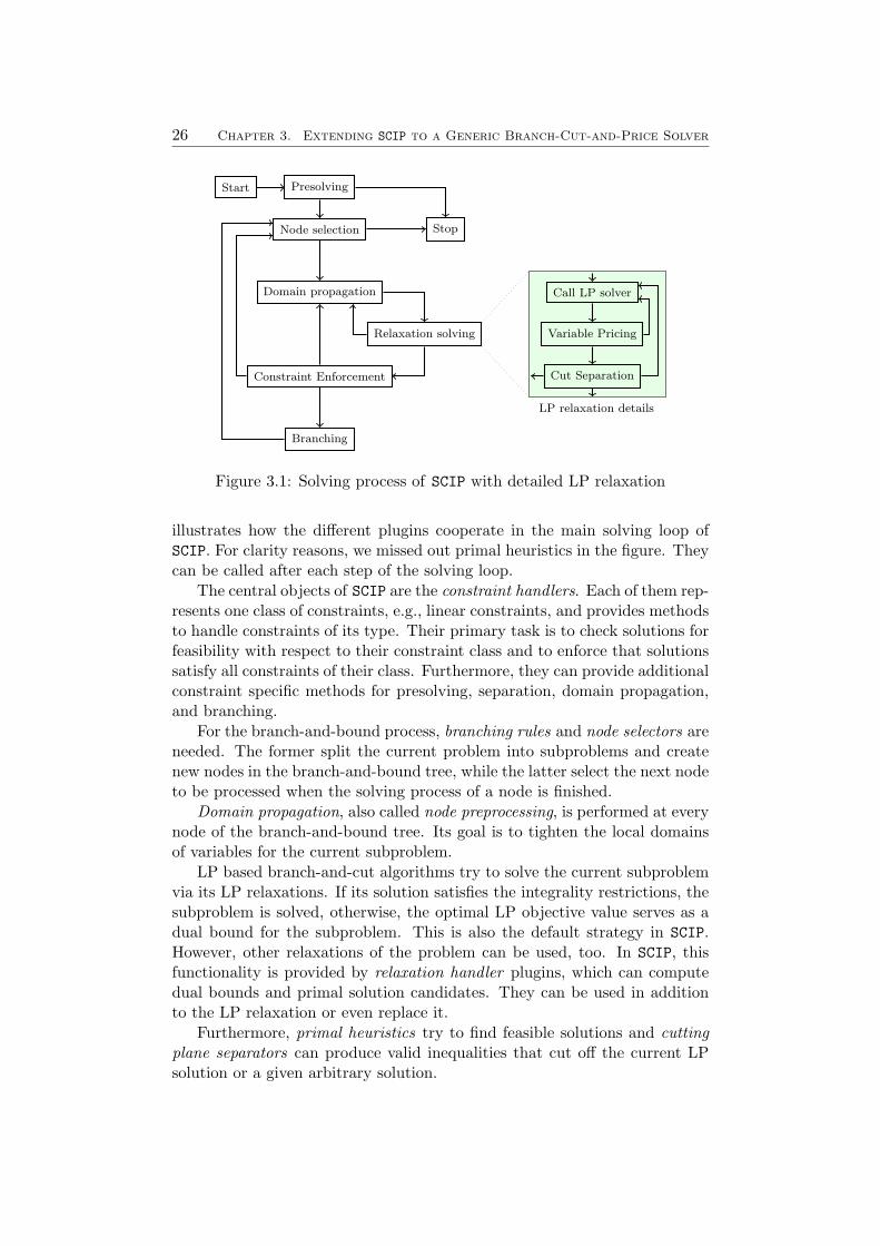
In the following, we give a short overview of the most important plugins.A detailed discussion of all types of plugins supported by SCIP and the un-derlying concepts can be found in [1, Chapter 3]. Furthermore, Figure 3.1
25
26 Chapter 3. Extending SCIP to a Generic Branch-Cut-and-Price Solver
Start Presolving
Node selection Stop
Domain propagation
Relaxation solving
Constraint Enforcement
Branching
Call LP solver
Variable Pricing
Cut Separation
LP relaxation details
Figure 3.1: Solving process of SCIP with detailed LP relaxation
illustrates how the different plugins cooperate in the main solving loop ofSCIP. For clarity reasons, we missed out primal heuristics in the figure. Theycan be called after each step of the solving loop.
The central objects of SCIP are the constraint handlers. Each of them rep-resents one class of constraints, e.g., linear constraints, and provides methodsto handle constraints of its type. Their primary task is to check solutions forfeasibility with respect to their constraint class and to enforce that solutionssatisfy all constraints of their class. Furthermore, they can provide additionalconstraint specific methods for presolving, separation, domain propagation,and branching.
For the branch-and-bound process, branching rules and node selectors areneeded. The former split the current problem into subproblems and createnew nodes in the branch-and-bound tree, while the latter select the next nodeto be processed when the solving process of a node is finished.
Domain propagation, also called node preprocessing, is performed at everynode of the branch-and-bound tree. Its goal is to tighten the local domainsof variables for the current subproblem.
LP based branch-and-cut algorithms try to solve the current subproblemvia its LP relaxations. If its solution satisfies the integrality restrictions, thesubproblem is solved, otherwise, the optimal LP objective value serves as adual bound for the subproblem. This is also the default strategy in SCIP.However, other relaxations of the problem can be used, too. In SCIP, thisfunctionality is provided by relaxation handler plugins, which can computedual bounds and primal solution candidates. They can be used in additionto the LP relaxation or even replace it.
Furthermore, primal heuristics try to find feasible solutions and cuttingplane separators can produce valid inequalities that cut off the current LPsolution or a given arbitrary solution.

3.2. GCG—a Generic Branch-Cut-and-Price Solver 27
Finally, variable pricers can add variables to the problem during the solv-ing process. Variables can be treated implicitly and added to the problemonly when needed. This concept is called column generation—see Chapter 4for a detailed discussion—and allows to implement branch-and-price algo-rithms in SCIP.
The current distribution of SCIP already contains a bundle of plugins thatcan be used for MIP solving. The most important ones are described in [1,Chapter 5 – 10]. SCIP with default plugins is a state-of-the-art MIP solverwhich is competitive (see Mittelmann’s “Benchmarks for Optimization Soft-ware” [67]) with other free solvers like CBC [31], GLPK [38], and Symphony [79]and also with commercial solvers like Cplex [43] and Gurobi [42]. Therefore,in order to compare the performance of our branch-cut-and-price solver GCGto a branch-and-cut MIP solver, we will use SCIP with default plugins as aMIP solver of this kind.
3.2 GCG—a Generic Branch-Cut-and-Price Solver
GCG (an acronym for “Generic Column Generation”) is an add-on for SCIPthat takes into account the structure of a MIP and solves it with a branch-cut-and-price approach after performing a Dantzig-Wolfe decomposion. Itwas developed by the author of this thesis. GCG supports both the convex-ification approach (see Section 2.1) as well as the discretization approach(Section 2.2). The description of the solving process and the structure ofGCG in the remainder of this section is valid for both these approaches. Dif-ferences that occur for the pricing, branching, and separation process arediscussed in the following three chapters. The most important parameters ofGCG described in the following are summarized in Appendix B.
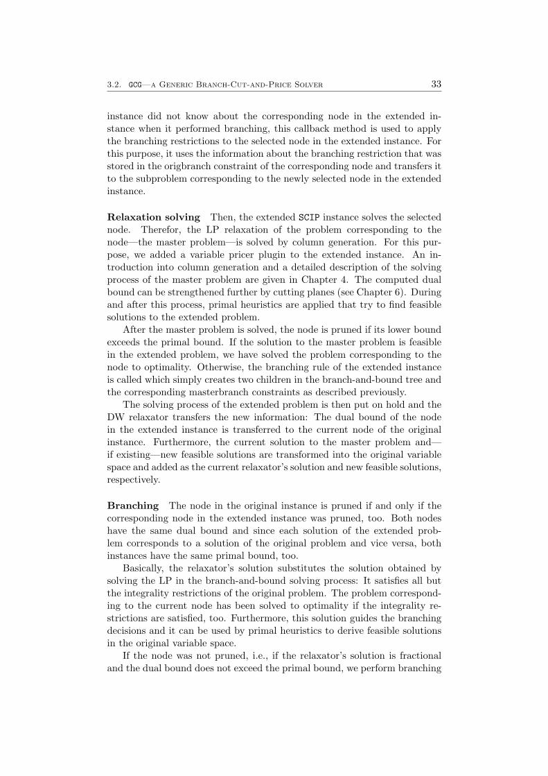
Even though the specifications of SCIP did not always allow a straightfor-ward implementation and sometimes lead to some overhead, by embeddingGCG into SCIP, we benefit from the efficient branch-and-bound frameworkwith all its sophisticated functionalities.
The general structure of GCG is the following: Besides the main SCIPinstance, that reads in the original problem, we use a second SCIP instancethat represents the extended problem. In the following, we will call theseinstances the original and the extended (SCIP) instance, respectively. Inaddition to these two SCIP instances, all pricing problems are represented bytheir own SCIP instance, too.
The original SCIP instance is the primary one which coordinates the solv-ing process, the extended SCIP instance is controlled by a relaxation handlerthat is included into the original SCIP instance. This relaxation handler iscalled DW relaxator in the following. The relaxator provides the two parame-ters usedisc and aggrblocks, that specify, whether the discretization approachshould be used for the decomposition and whether identical blocks should beaggregated, respectively.

28 Chapter 3. Extending SCIP to a Generic Branch-Cut-and-Price Solver
original SCIP instance extended SCIP instance
Start Presolving
Decomposition
Node selection Stop
Domain propagation
Solve relaxation
Transfer solution
Constraint Enforcement
Branching
Select corresponding nodeand apply branching changes
Domain propagation
Solve master problemwith column generation
and cut separation
Constraint Enforcement
Branching
Figure 3.2: Solving process of GCG
The structure of GCG can be interpreted in the following way: We treatthe original problem as the essential one, by actually solving it with a “stan-dard” branch-and-bound method, like it is done by most state-of-the-art MIPsolvers. The only difference is, that we do not use the LP relaxation to com-pute lower bounds and corresponding primal solution candidates, but anotherrelaxation, namely the master problem. Hence, the original SCIP instancecoordinates the solving process while the extended instance is only used torepresent and solve the relaxation.
In the following, we survey the solving process of GCG, the most importantparts are described in detail in the following chapters. The main solving loopof GCG is illustrated in Figure 3.2.
Dantzig-Wolfe decomposion In the current version of GCG, informationabout the structure of the problem has to be provided in an additional filethat is read in after reading the MIP. In particular, the number of blocksin the constraint matrix and the variables corresponding to each block canbe specified in this file. In addition to that, constraints can be explicitlylabelled to be linking constraints (see (2.1) in Model 2.1), which forces theseconstraints to be transferred to the extended problem (see Model 2.4, 2.8,and 2.10). In the following, we describe the decomposition and the setup ofthe SCIP instances, an ilustration is given in Figure 3.3.
After the original instance has finished its presolving process, the relax-ator performes the Dantzig-Wolfe decomposion and initializes the extended

3.2. GCG—a Generic Branch-Cut-and-Price Solver 29
original SCIP instanceextended
SCIP instance
pricing SCIPinstance 1 pricing SCIP
instance 2
pricing SCIPinstance 3
variables ofblock 1
variables ofblock 2
variables ofblock 3
label
led
linkin
gco
nst
rain
ts
convex
ity
const
rain
ts
Figure 3.3: Example for the decomposition process of the original problem’sconstraint matrix. We miss out the right-hand sides of the linear constraintfor the sake of clarity. Note that the extended SCIP instance does not containany variables right from the beginning so the corresponding constraints doneither.
SCIP instance as well as the SCIP instances representing the pricing prob-lems. Initially, the extended instance does contain neither constraints norvariables. The variables that are labelled to be part of a block are copiedand added to the corresponding pricing problem: For each constraint of theoriginal instance, it is determined whether it only contains variables of oneblock. If this is the case, the constraint is regarded as a structural constraintof this block and added to the corresponding pricing problem. Otherwise, itis viewed as a linking constraint, transformed according to the Dantzig-Wolfereformulation and added to the extended instance. If a constraint is explic-itly labeled to be a linking constraints, it will be transferred to the extendedinstance even if all contained variables belong to the same block. Further-more, the convexity constraints (see e.g., (2.11) in Model 2.4) are created inthe extended problem.
We do not add variables to the extended instance in this process. This isonly done in the solving process of the master problem. Hence, we do not onlyuse a restricted master problem, but we also restrict the extended problem tothe same set of variables. Therefore, the constraints in the extended problemdo not explicitly contain any variables at the beginning, but they implicitlyknow the coefficients of all implicitly given variables.

30 Chapter 3. Extending SCIP to a Generic Branch-Cut-and-Price Solver
When using the discretization approach and aggregation of blocks, iden-tical blocks are identified during the reformulation process and aggregated.We provide a rather basic check for identity, i.e., in the problem definition,constraints and variables have to be defined in the same sequence for identi-cal blocks. Much more sophisticated methods could be used for this process,but that was not the aim of this thesis.
Coordination of the branch-and-bound trees During the solving pro-cess, the extended instance builds the same branch-and-bound tree as theoriginal instance. Each node of the original instance corresponds to a nodeof the extended instance. In the following, we describe, how this is estab-lished. An illustration is given in Figure 3.4.
The connection between a node in the original instance and the corre-sponding node in the extended instance is established by additional constrainthandlers in the original and the extended instance. In a slight abuse of theproper sense of constraint handlers, they do not handle problem restrictionsbut establish the coordination of both branch-and-bound trees. In the follow-ing, we will call the constraint handler in the original instance the origbranchconstraint handler and the one in the extended instance the masterbranchconstraint handler. The corresponding constraints are called origbranch andmasterbranch constraints, respectively. These constraints are added to thenodes of the original and extended instance, respectively, to synchronize thesolving process of both instances.
Each origbranch constraint knows the node in the original instance itbelongs to and the origbranch constraints associated with the father and thechildren of this node in the branch-and-bound tree. Furthermore, it containsa pointer to the masterbranch constraint of the corresponding node in theextended instance. Each masterbranch constraint knows about the nodein the extended instance to which it belongs, the masterbranch constraintscorresponding to its father and its children and the origbranch constraint ofthe corresponding node in the original instance.
We need this overhead, since we cannot create branch-and-bound nodesof two SCIP instances at the same time. Nodes of one instance can only becreated by a branching rule plugin included in this instance.
When branching in the extended instance (see step 2 in Figure 3.4), wejust create two children without imposing any further branching restrictions.To each of these children, a masterbranch constraint is added and pointersto these constraints are stored in the masterbranch constraint of the currentnode. The masterbranch constraints of the child nodes only know the nodethey belong to as well as the masterbranch constraint corresponding to theirfather node. The connection to the origbranch constraint of the correspond-ing node in the original instance is established later.
In a subsequent step, branching is performed at the corresponding nodein the original instance (see step 3 in Figure 3.4). The branching rule ofthe original instance creates two child nodes, too. To these child nodes,

3.2. GCG—a Generic Branch-Cut-and-Price Solver 31
1. Connection between the two current nodes established,solve the master problem
...
...
2. Perform branching in the extended SCIP instance...
...
3. Perform branching in the original SCIP instance (if needed)
...
...
4. Select next node in the original SCIP instance
...
...
5. Select the corresponding node in the extended SCIP instance,establish the connection between the nodes
...
...
Figure 3.4: The coordination of the branch-and-bound trees. The branch-and-bound tree of the original SCIP instance is pictured on the left side, theone of the extended instance on the right side. We identify the origbranch andmasterbranch constraints with the branch-and-bound nodes and representthe pointers stored at the constraints by the dotted lines.

32 Chapter 3. Extending SCIP to a Generic Branch-Cut-and-Price Solver
origbranch constraints are added. Like the masterbranch constraints, theyinitially only know about the corresponding node in the original instance andthe origbranch constraint of the father node. Furthermore, the branching ruleimposes restrictions on the (original) subproblems corresponding to the childnodes.
The corresponding subproblems in the extended instance were createdwithout any restrictions. In order to transfer the restrictions imposed on theoriginal subproblems to the corresponding nodes in the extended instance,the original branching rule can store information about these restrictionsat the origbranch constraints added to the child nodes. Furthermore, itcan provide callback functions that are called when a node in the extendedinstance is activated. These callback functions can be used to finally enforcethe branching restrictions in the subproblems of the corresponding nodes inthe extended instance. More details about these callback functions and howthe branching rules incorporated in GCG use them can be found in Chapter 5.
Node selection We currently use the default node selection rule of SCIP inthe original instance, which realizes a best first search. When solving a nodein the branch-and-bound tree of the original SCIP instance, the lower bound ofthe node is not computed by solving its LP relaxation, but the DW relaxatoris called for this purpose. It instructs the extended SCIP instance to continueits solving process. A special node selector in the extended instance choosesas the next node to be processed the node corresponding to the current nodein the original instance. Its subproblem is always a valid reformulation of thesubproblem corresponding to the current node in the original instance.
As described previously, the connection between the nodes was not yetestablished. It is established by the node selector when it activates the nodein the extended instance that corresponds to the current node in the originalinstance. The origbranch constraint corresponding to the current node inthe original instance knows the origbranch constraint of its father node. Ifthere does not exist a father node, then the current node is the root nodeand the node selector activates the root node in the extended instance, too.Otherwise, the father node was activated before and the corresponding orig-branch constraint already knows the corresponding masterbranch constraint.If the current node in the original problem is a left child, then the nodeselector activates in the extended problem the left child of the node corre-sponding to the father node of the current node in the original problem (seestep 5 in Figure 3.4). Otherwise, it chooses the right child of the node inthe extended problem corresponding to the father node. Furthermore, theorigbranch and the masterbranch constraints corresponding to the selectednodes in the original and extended instance, respectively, store the pointerto each other.
When the node in the extended instance is activated, one of the pre-viously mentioned callback methods, that is defined by the branching rulein the original instance, is called. Since the branching rule in the original
3.2. GCG—a Generic Branch-Cut-and-Price Solver 33
instance did not know about the corresponding node in the extended in-stance when it performed branching, this callback method is used to applythe branching restrictions to the selected node in the extended instance. Forthis purpose, it uses the information about the branching restriction that wasstored in the origbranch constraint of the corresponding node and transfers itto the subproblem corresponding to the newly selected node in the extendedinstance.
Relaxation solving Then, the extended SCIP instance solves the selectednode. Therefor, the LP relaxation of the problem corresponding to thenode—the master problem—is solved by column generation. For this pur-pose, we added a variable pricer plugin to the extended instance. An in-troduction into column generation and a detailed description of the solvingprocess of the master problem are given in Chapter 4. The computed dualbound can be strengthened further by cutting planes (see Chapter 6). Duringand after this process, primal heuristics are applied that try to find feasiblesolutions to the extended problem.
After the master problem is solved, the node is pruned if its lower boundexceeds the primal bound. If the solution to the master problem is feasiblein the extended problem, we have solved the problem corresponding to thenode to optimality. Otherwise, the branching rule of the extended instanceis called which simply creates two children in the branch-and-bound tree andthe corresponding masterbranch constraints as described previously.
The solving process of the extended problem is then put on hold and theDW relaxator transfers the new information: The dual bound of the nodein the extended instance is transferred to the current node of the originalinstance. Furthermore, the current solution to the master problem and—if existing—new feasible solutions are transformed into the original variablespace and added as the current relaxator’s solution and new feasible solutions,respectively.
Branching The node in the original instance is pruned if and only if thecorresponding node in the extended instance was pruned, too. Both nodeshave the same dual bound and since each solution of the extended prob-lem corresponds to a solution of the original problem and vice versa, bothinstances have the same primal bound, too.
Basically, the relaxator’s solution substitutes the solution obtained bysolving the LP in the branch-and-bound solving process: It satisfies all butthe integrality restrictions of the original problem. The problem correspond-ing to the current node has been solved to optimality if the integrality re-strictions are satisfied, too. Furthermore, this solution guides the branchingdecisions and it can be used by primal heuristics to derive feasible solutionsin the original variable space.
If the node was not pruned, i.e., if the relaxator’s solution is fractionaland the dual bound does not exceed the primal bound, we perform branching
34 Chapter 3. Extending SCIP to a Generic Branch-Cut-and-Price Solver
in the original instance and create two children as described previously. Thebranching decisions will be transferred to the corresponding nodes in theextended problem later. Different possibilities to perform branching in thiscontext are presented in Chapter 5.
After branching, the original SCIP instance selects a node that is solvednext and the process is iterated.
An alternative interpretation of the branch-cut-and-price process
Like stated previously, we treat the original instance as the essential oneand actually solve it with a “standard” branch-and-bound method. The LPrelaxation is substituted by the DW relaxator that uses the extended SCIPinstance to solve the master problem.
Anyhow, solving a MIP using the Dantzig-Wolfe decomposion and branch-cut-and-price can also be interpreted in another way: The problem that isactually solved is the extended problem, we only need the original problem toensure integrality of the solution in the original variable space and to guidebranching decisions. Thus, another possible structure for the implementationwould have been to make the extended instance the coordinating one and tostore the original problem only for the previously mentioned purposes.
For the discretization approach, integrality can even be directly enforcedin terms of the variables of the extended formulation and branching is oftenperformed in terms of these variables as well (see Chapter 5). Hence, wecould actually forget about the original problem, solve the extended problemto optimality by branch-cut-and-price and transfer the optimal solution ofthe extended problem to the original problem afterwards.
Motivation for the employed structure
We had to weight these possibilities against each other and we chose theformer one for our implementation since it fits better into the SCIP frameworkand makes better use of the functionalities already provided by SCIP. Theoriginal problem can be read in by the original instance using the default filereader plugins provided by SCIP, so there is a variety of formats that canbe read in. If we do not read an additional file defining the structure of theproblem, the problem is solved by SCIP with a branch-and-cut algorithm.
On the other hand, if we read such an additional file, the DW relaxator isactivated, it creates the second SCIP instance, performes the Dantzig-Wolfedecomposion and substitutes the LP relaxation in the branch-and-bound pro-cess. Furthermore, by choosing this structure, we solve both problems simul-taneously and can transfer information from one problem to the other duringthe solving process. Hence, techniques that speed up the solving process,e.g., presolving and domain propagation, can be used in both instances.
We provide possibilities to use either the convexification or the discretiza-tion approach, so we had to make sure, that the structure of the implemen-tation fits for both approaches. For the convexification approach, the first

3.3. Computational Environment 35
interpretation is the more natural structure, anyway, since integrality is de-fined in terms of the original variables. For the discretization approach, wecan define branching rules that branch in terms of the variables in the ex-tended problem and do not change the original problem explicitly, turningthe implementation into an algorithm that essentially realizes the secondinterpretation.
However, we do not forget about the original problem and under certainconditions, we can conclude that a problem is solved to optimality due to theadditional information provided by the original problem: If we only used theextended problem and the solution to the master problem was fractional, wewould perform branching unless the node can be pruned. Anyhow, a frac-tional solution of the master problem may correspond to an integral solutionof the original problem, like in the convexification approach. In this case, wehave solved the current subproblem since this original integral solution canbe retransferred into an optimal solution of the current extended problem.
3.3 Computational Environment
For the computational experiments presented in the following chapters con-cerning the pricing process (Section 4.4), different branching schemes (Sec-tion 5.7), and the separation of cutting planes (Section 6.4), and for finalresults and comparisons to SCIP (Chapter 7), we used four classes of prob-lems: The bin packing problem (BPP), the vertex coloring problem (VCP),the capacitated p-median problem (CPMP), and a resource allocation problem(RAP).
Problem definitions and the different test sets for each of the problemclasses are presented in Appendix C. For each test set, we also defined asmall test set containing less instances. In order to reduce the computationaleffort, we used these test sets in all computations concerning the performanceeffect of certain features of GCG. As some of these small test sets were definedwith respect to the performance of GCG for the single instances, we did notuse them for the comparison of GCG and SCIP. In this context, we usedthe complete test sets; the results are presented in Section 7.4. We presentsummaries of the results in the according chapters and interpret the results.Detailed results of the computations can be looked up in Appendix D.
For all computations presented in this thesis, we used GCG version 0.7.0and SCIP version 1.2.0.5, which were compiled with gcc 4.4.0 with the-O3 optimizer option under openSUSE 11.2 (64 Bit). Cplex 12.1 [43] wasalways used as underlying LP solver for solving the LP relaxations.
The computational tests described in Section 4.4 and 6.4 were carried outon a 3 GHz Intel Xeon with 4 MB cache and 8 GB RAM. In the remainingchapters, the computations for the BPP and the VCP were performed on a3.60 GHz Intel Pentium D with 2 MB cache and 4 GB RAM, those for theCPMP on a 2.66 GHz Intel Core 2 Quad with 4 MB cache and 4 GB RAM.

36 Chapter 3. Extending SCIP to a Generic Branch-Cut-and-Price Solver
The computations for the RAP test sets were performed on a 2.83 GHz IntelCore 2 Quad with 6 MB cache and 16 GB RAM.
When summarizing the results and not listing individual results for eachsingle instance, we report average values for each test set. However, thereare different possibilities to define the average values.
Since the values for the instances in our test sets differ highly in theirmagnitude, we use the shifted geometric mean. For non-negative numbersa1, . . . , ak ∈ R+, for instance the number of nodes or the final gap of theindividual instances of a test set, and a shift s ∈ R+, it is defined as
γs(a1, . . . , ak) =
(k∏
i=1
max{ai + s, 1}
) 1k
− s.
It focuses on ratios instead of totals, so it does not overestimate the hugenumbers, as it is done by the arithmetic mean. By shifting the values, weprevent the smaller numbers from having a bigger influence which is oftenencountered for the geometric mean. For a more detailed description andcomparison of these three possibilities to compute averages, we refer to [1].
In the summary tables in the following chapters and also in Tables D.1to D.30 in Appendix D, we just list shifted geometric means for each testset, only the number of timeouts is always given in absolute numbers. Alltime measurements are given in seconds. We often present percental changesof some settings compared to a “default” setting. In this case, we highlightchanges of at least five percent by printing them blue if they represent animprovement and red in case of a deterioration.
We use a shift of s = 5 for the LP solving time, s = 10 for pricing time,solving time of the master problem and total time as well as for the numberof nodes. A shift s = 100 is used for the number of pricing problems thatare solved, the number of pricing rounds, the number of variables createdin the master problem, and the final gap in percent. We used the smallshifts for time and nodes since many of the regarded problems are solvedin a small amount of time and after a small number of nodes. The othernumbers are typically higher so we also used a greater shift. Since all shiftsare larger than 1, the maximum in the definition of the shifted geometricmean is always achieved for the first value, so the shifted geometric mean isactually given as
γs(a1, . . . , ak) =
(k∏
i=1
(ai + s)
) 1k
− s.
We define the final gap of an instance by |pb−db||db| with pb and db being the
global primal and dual bound, respectively, at the moment when the solvingprocess was stopped. The dual bound db is always positive for the instanceswe regarded, so we do not divide by zero. However, if we did not find a
3.3. Computational Environment 37
solution for the instance within the time limit, the gap for this instance isinfinity, denoted by a “–” in the tables. In this case, we charged a gap of100% for the computation of the average. For general MIPs, this value isoften exceeded and would therefore not be a good choice, for the problemclasses that we examined in this thesis, however, final gaps larger than thatdid not occur.
In the summary tables, we typically list the shifted geometric mean foreach test set. In order to get an average number over all test sets, we computethe shifted geometric mean of the mean values for the single test sets. Sincethe test sets have different sizes (the small test sets range from 12 to 28instances), the single instances from the smaller test sets have a greaterinfluence on the overall average. This is intended as we want to give the sameweight to each test set. Furthermore, since we defined multiple test sets forsome of the problem classes treated in this thesis, these classes of problemsare overrepresented in the computation of the average values. However, thedifferent test sets for one class typically differ from each other in terms ofproblem size so we decided to treat each size the same way as all other testsets. If there are big differences between the results for different classes ofproblems, we name these differences, anyhow, and do not just consider theaverage value.

38 Chapter 3. Extending SCIP to a Generic Branch-Cut-and-Price Solver

Chapter 4
Solving the Master Problem
As described previously, we solve the original and the extended problemsimultaneously. In order to compute dual bounds, we use the LP relaxationof the extended formulation, which we called the master problem (Model 2.5,Model 2.9, or Model 2.14 for the different approaches). As the extendedformulation has an exponential number of variables, the master problem doesso, too. In this chapter, we describe how we solve the master problem despitethis.
We present the concept of column generation (sometimes also called de-layed column generation) in Section 4.1, which is a method to solve LPs witha huge number of variables. Instead of treating all variables explicitly, onlya small subset of variables is added to the LP, the remaining variables areconsidered implicitly and added to the LP only when needed.
In Section 4.2, we illustrate how this concept can be used to solve themaster problem obtained by the Dantzig-Wolfe decomposition. After that,in Section 4.3, we describe the integration into the generic branch-cut-and-price framework GCG and discuss implementational details. Finally, in Sec-tion 4.4, we present computational results for the pricing process based onthe problems classes presented in Appendix C.
4.1 Basics in Column Generation
Column generation is a method for solving linear programs with typically ahuge number of variables but a reasonable number of constraints.
It is mostly used for solving the LP relaxation of certain (mixed-)integerprograms where the variables are not given explicitly but by a specific struc-ture (see [27]). In the set partitionig formulation of the bin packing problem(see Section C.1), for instance, we define a binary variable for each feasiblepacking of a bin, that is a set of items that can be assigned to a bin withoutexceeding its capacity. There is a huge number of these packings, so we donot want to enumerate all of them but treat them implicitly.
In this section, we focus on the solution process of such an LP, which is
39
40 Chapter 4. Solving the Master Problem
an important basis for the concepts presented in this thesis.We start with an LP that explicitly contains all variables. This problem
is called the master problem (MP).
Model 4.1 (Master Problem)
zMP = min cTx
s.t. Ax ≥ a (4.1)Bx = b (4.2)x ∈ Qn
+
with c ∈ Qn, A ∈ Qm×n, B ∈ Qp×n, a ∈ Qm, and b ∈ Qp.
In Chapter 2, we also defined master problems, namely the LP relaxationsof the extended fomulations. We did so, since we will solve these problems—which are also LPs with an exponential number of variables—using columngeneration (see Section 4.2). In this process, they will be the counterpart ofModel 4.1. In this section, however, we regard the general master problemdefined in Model 4.1.
Storing the whole LP explicitly in the memory of a computer is typi-cally impossible due to the enormous number of variables, so we restrict theproblem to a subset of the variables and add variables to this subset onlywhen needed. The resulting problem is called the restricted master problem(RMP).
Model 4.2 (Restricted Master Problem)
zRMP = min cNxN
s.t. A·,NxN ≥ a (4.3)B·,NxN = b (4.4)
xN ∈ Q|N |+
with N ⊆ {1, . . . , n}
In order to define subsets of vectors and matrices, we normally need anordered set. As we do not need a special ordering in this section, we assumethe set N to be ordered increasingly and use it in a slight abuse of notationin order to define subvectors and submatrices.
Each solution to the RMP is also a solution to the master problem, if weset all variables not contained in the master problem to 0. In the following,we assume that this is done whenever we speak of solutions of the RMP thatare regarded with respect to the master problem. An optimal solution to theRMP, however, may be suboptimal in the master problem, since considering

4.1. Basics in Column Generation 41
Solve RMP
Farkas Pricing Reduced Cost Pricing
MP infeasible MP unboundedFound optimalsolution for MP
no variablesadded
no variablesadded
RMPunbounded
RMPinfeasible
RMP hasoptimal solu-tion
new variableadded
new variableadded
Figure 4.1: The solving process of the master problem
the whole set of variables could lead to a better solution. Nevertheless, westart the solving process of the master by solving the RMP to optimality.
If the RMP is primally unbounded, then this also holds for the masterproblem (see Theorem 4.7 at the end of this section). We can stop the solvingprocess since we have proven the master problem to be unbounded.
If the RMP is primal infeasible, the master problem might also be primalinfeasible. In most cases, however, we only have to add some variables to theset N in order to restore feasibility. In particular, when solving the RMPthe first time, we can start without variables, i.e., N = ∅, so the RMP isinfeasible if a 6≤ 0 or b 6= 0. The process that looks for variables that canhelp to restore feasibility is called Farkas pricing [41, 16] in the following.
In case we get an optimal primal solution to the RMP, we do not knowwhether it is also optimal for the master problem. Hence, we have to look forvariables in the master problem, that could improve that solution and addthese variables to the set N of variables of the RMP. We refer to this processas reduced cost pricing since we look for variables with negative reduced costs.
After variables have been added, the RMP is resolved and the process isiterated. This is repeated, until no more variable can improve the currentsolution or can help to fix an infeasibility. If the RMP is still infeasible, thenthe master problem is infeasible, too. If the RMP has an optimal solution,then this solution is also optimal for the master problem. We will prove thesestatements at the end of this section.
The solving process of the master problem is illustrated in Figure 4.1.Once the RMP is feasible, it stays feasible since adding variables conserves
feasibility. Hence, Farkas pricing is used until the RMP gets feasible, afterthat, we use nothing but reduced cost pricing.
In the next two subsections, we specify how the two pricing types workexactly, starting with reduced cost pricing and concluding with Farkas pric-
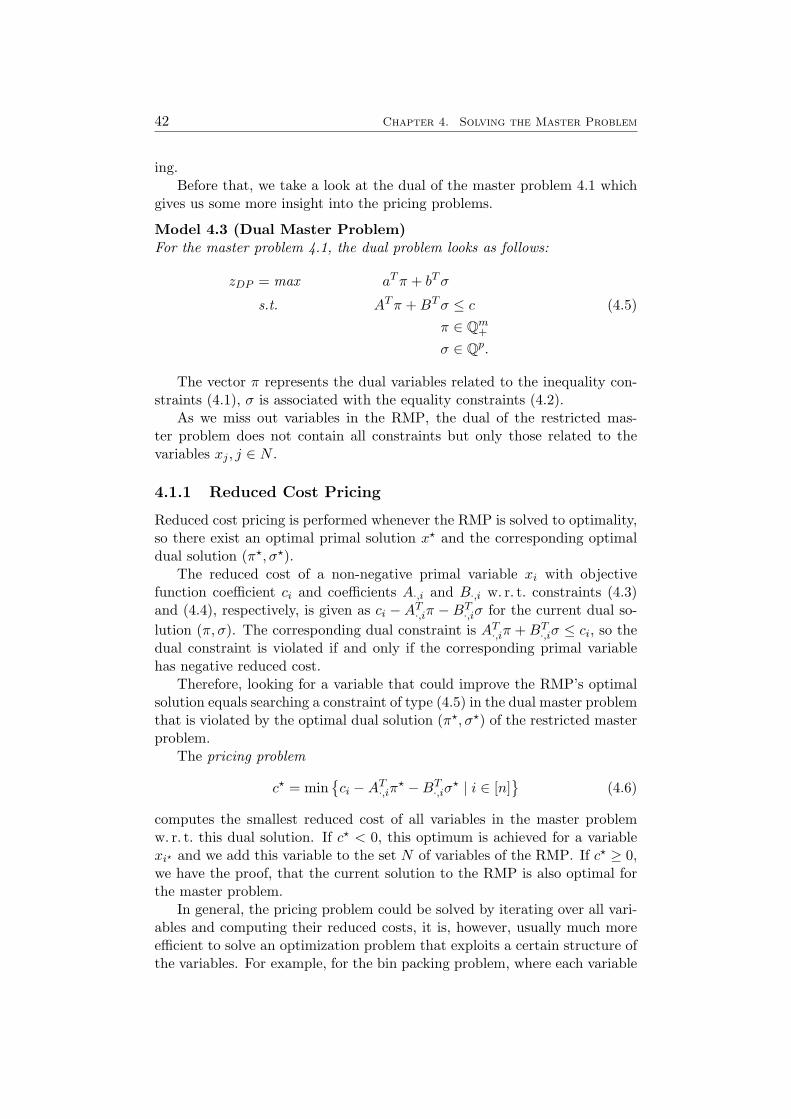
42 Chapter 4. Solving the Master Problem
ing.Before that, we take a look at the dual of the master problem 4.1 which
gives us some more insight into the pricing problems.
Model 4.3 (Dual Master Problem)For the master problem 4.1, the dual problem looks as follows:
zDP = max aTπ + bTσ
s.t. ATπ +BTσ ≤ c (4.5)π ∈ Qm
+
σ ∈ Qp.
The vector π represents the dual variables related to the inequality con-straints (4.1), σ is associated with the equality constraints (4.2).
As we miss out variables in the RMP, the dual of the restricted mas-ter problem does not contain all constraints but only those related to thevariables xj , j ∈ N .
4.1.1 Reduced Cost Pricing
Reduced cost pricing is performed whenever the RMP is solved to optimality,so there exist an optimal primal solution x? and the corresponding optimaldual solution (π?, σ?).
The reduced cost of a non-negative primal variable xi with objectivefunction coefficient ci and coefficients A·,i and B·,i w. r. t. constraints (4.3)and (4.4), respectively, is given as ci − AT
·,iπ − BT·,iσ for the current dual so-
lution (π, σ). The corresponding dual constraint is AT·,iπ +BT
·,iσ ≤ ci, so thedual constraint is violated if and only if the corresponding primal variablehas negative reduced cost.
Therefore, looking for a variable that could improve the RMP’s optimalsolution equals searching a constraint of type (4.5) in the dual master problemthat is violated by the optimal dual solution (π?, σ?) of the restricted masterproblem.
The pricing problem
c? = min{ci −AT
·,iπ? −BT
·,iσ? | i ∈ [n]
}(4.6)
computes the smallest reduced cost of all variables in the master problemw. r. t. this dual solution. If c? < 0, this optimum is achieved for a variablexi? and we add this variable to the set N of variables of the RMP. If c? ≥ 0,we have the proof, that the current solution to the RMP is also optimal forthe master problem.
In general, the pricing problem could be solved by iterating over all vari-ables and computing their reduced costs, it is, however, usually much moreefficient to solve an optimization problem that exploits a certain structure ofthe variables. For example, for the bin packing problem, where each variable
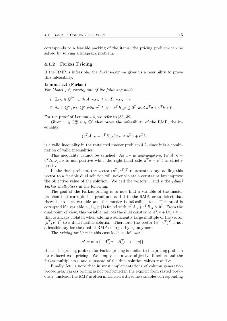
4.1. Basics in Column Generation 43
corresponds to a feasible packing of the items, the pricing problem can besolved by solving a knapsack problem.
4.1.2 Farkas Pricing
If the RMP is infeasible, the Farkas-Lemma gives us a possibility to provethis infeasiblity.
Lemma 4.4 (Farkas)For Model 4.2, exactly one of the following holds:
1. ∃xN ∈ Q|N |+ with A·,NxN ≥ a, B·,NxN = b
2. ∃u ∈ Qm+ , v ∈ Qp with uTA·,N + vTB·,N ≤ 0T and uTa+ vT b > 0.
For the proof of Lemma 4.4, we refer to [85, 39].Given u ∈ Qm
+ , v ∈ Qp that prove the infeasiblity of the RMP, the in-equality
(uTA·,N + vTB·,N )xN ≥ uTa+ vT b
is a valid inequality in the restricted master problem 4.2, since it is a combi-nation of valid inequalities.
This inequality cannot be satisfied: As xN is non-negative, (uTA·,N +vTB·,N )xN is non-positive while the right-hand side uTa + vT b is strictlypositive.
In the dual problem, the vector (uT , vT )T represents a ray; adding thisvector to a feasible dual solution will never violate a constraint but improvethe objective value of the solution. We call the vectors u and v the (dual)Farkas multipliers in the following.
The goal of the Farkas pricing is to now find a variable of the masterproblem that corrupts this proof and add it to the RMP, or to detect thatthere is no such variable and the master is infeasible, too. The proof iscorrupted if a variable xi, i ∈ [n] is found with uTA·,i+vTB·,i > 0T . From thedual point of view, this variable induces the dual constraint AT
·,iπ+BT·,iσ ≤ ci
that is always violated when adding a sufficiently large multiple of the vector(uT , vT )T to a dual feasible solution. Therefore, the vector (uT , vT )T is nota feasible ray for the dual of RMP enlarged by xi, anymore.
The pricing problem in this case looks as follows:
c? = min{−AT·,iu−BT
·,iv | i ∈ [n]}.
Hence, the pricing problem for Farkas pricing is similar to the pricing problemfor reduced cost pricing. We simply use a zero objective function and thefarkas multipliers u and v instead of the dual solution values π and σ.
Finally, let us note that in most implementations of column generationprocedures, Farkas pricing is not performed in the explicit form stated previ-ously. Instead, the RMP is often initialized with some variables corresponding

44 Chapter 4. Solving the Master Problem
to a previously computed heuristic solution or with artificial variables thatare penalized by a big M cost, like in the the simplex first phase. However,due to the generic approach presented in this thesis, we restrict ourselves toFarkas pricing for restoring feasibility of the RMP.
4.1.3 Finiteness and Correctness
We conclude this section with two theorems proving the finiteness and thecorrectness of the column generation procedure as described above.
Theorem 4.5 (Finiteness of the column generation process)The column generation process terminates after a finite number of iterations.
Proof 4.6In each iteration, we either are finished and stop or add at least one variableof the master problem to the restricted master problem.
Since the number of variables in the master problem is finite, it is suffi-cient to show that each variable is added to the RMP at most once.
When performing reduced cost pricing, we add a variable xi? to the RMPonly if the optimum c? of (4.6) is achieved for i? and c? < 0. Since c? equalsthe reduced cost of xi?, xi? has negative reduced cost. The current solution tothe RMP, however, is optimal and thus, there exists no variable in the RMPwith negative reduced cost. Therefore, xi? was not part of the RMP before.
In the case of Farkas pricing, a variable is added only if it corrupts the in-feasibility proof given by u and v. For the dual of the current RMP, (uT , vT )T
forms a ray; the variable that is added corresponds to a new constraint in thedual of the RMP that limits this ray. If the variable that is added was partof the RMP before, the corresponding dual constraint would have been part ofthe RMP’s dual before, too. This is not possible since (uT , vT )T is a ray inthe dual of the current RMP. 2
Theorem 4.7 (Equivalence of master problem and RMP)After the column generation process has finished, the following holds:
• The RMP is unbounded if and only if the master problem is unbounded.
• The RMP is infeasible if and only if the master problem is infeasible.
• The RMP has an optimal solution if and only if the master problemhas an optimal solution and each optimal solution to the RMP is alsooptimal for the master problem.
Proof 4.8The column generation procedure can be interpreted as a generalization of thesimplex method. Instead of explicitly enumerating all variables to find onewith negative reduced cost, the pricing step of the simplex method is implicitlyperformed by solving the pricing problem. However, we give a formal prooffor the equivalence in the following.

4.2. Solving the Dantzig-Wolfe Master Problem 45
• If the RMP is unbounded, there exist a ray r ∈ Q|N |+ with cNr < 0,A·,Nr ≥ 0, and B·,Nr = 0 that proves the unboundedness. Let r ∈ Qn
+
with ri = rj if i = Nj and ri = 0, if i /∈ N . Then r is a ray in the masterproblem proving its unboundedness: cr = cNr < 0, Ar = A·,Nr ≥ 0,and Br = B·,Nr = 0. Hence, the master problem is also unbounded.
• If the RMP is infeasible, then there exist a vector (uT , vT )T that provesthe infeasibility (see Section 4.1.2). This vector represents a ray in thedual of the RMP with strictly positive objective function value. Thedual of the RMP contains the same variables as the dual of the masterproblem—the RMP contains all constraints—but only a subset of theconstraints, since the RMP does not contain all variables contained inthe master problem.
The column generation process is finished, so we did not add a variablein the last pricing round. Since the RMP is infeasible, we performedFarkas pricing and searched for a variable xi in the master satisfyinguTA·,i+vTB·,i > 0T . We did not add a variable to the RMP, thus, suchvariable does not exist in the master problem. So in the dual of the mas-ter problem, adding (uT , vT )T to a feasible solution preserves feasibilityas it does not increase the left-hand side of any of the constraints.
Thus, (uT , vT )T is also a feasible ray in the dual of the master problemwith strictly positive objective function value. Therefore, the masterproblem is infeasible, too.
• Let the RMP have an optimal solution. As the RMP is feasible andthe column generation process is finished, we performed reduced costpricing in the last pricing round but did not add a variable.
For the optimal solution of the RMP, we get a corresponding solutionx in the master problem by setting the solution values of all variablesnot contained in the RMP to 0. This solution is also a basic solution,so we can perform a simplex iteration in order to improve it. In thesimplex method, we search for a variable in the master that has negativereduced cost w. r. t. x. This is exactly what was done in the last pricinground and since no variable was added to the RMP, all variables in themaster have non-negative reduced cost. Due to the optimality criterionof the simplex method, x is an optimal solution of the master problem.
4.2 Solving the Dantzig-Wolfe Master Problem
When applying the Dantzig-Wolfe decomposition to a problem like describedin Chapter 2, we get an extended problem with typically an exponentialnumber of variables. Now, we describe how the master problem—the LPrelaxation of this problem—is solved with a column generation approach.
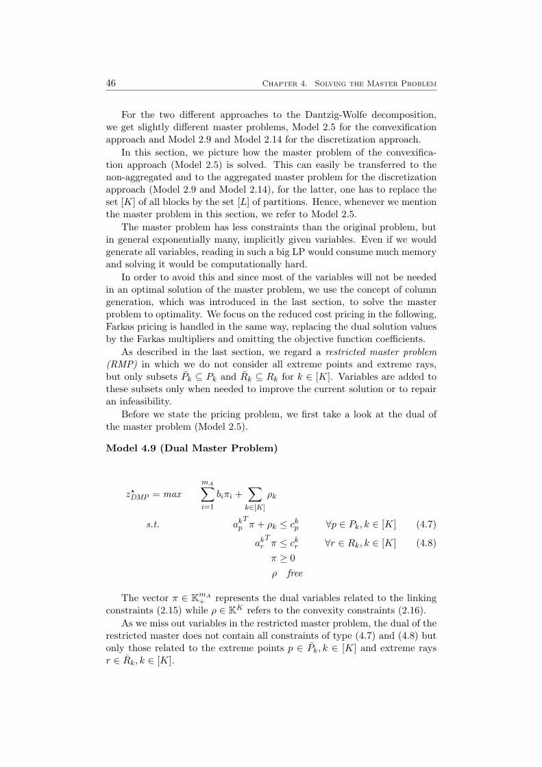
46 Chapter 4. Solving the Master Problem
For the two different approaches to the Dantzig-Wolfe decomposition,we get slightly different master problems, Model 2.5 for the convexificationapproach and Model 2.9 and Model 2.14 for the discretization approach.
In this section, we picture how the master problem of the convexifica-tion approach (Model 2.5) is solved. This can easily be transferred to thenon-aggregated and to the aggregated master problem for the discretizationapproach (Model 2.9 and Model 2.14), for the latter, one has to replace theset [K] of all blocks by the set [L] of partitions. Hence, whenever we mentionthe master problem in this section, we refer to Model 2.5.
The master problem has less constraints than the original problem, butin general exponentially many, implicitly given variables. Even if we wouldgenerate all variables, reading in such a big LP would consume much memoryand solving it would be computationally hard.
In order to avoid this and since most of the variables will not be neededin an optimal solution of the master problem, we use the concept of columngeneration, which was introduced in the last section, to solve the masterproblem to optimality. We focus on the reduced cost pricing in the following,Farkas pricing is handled in the same way, replacing the dual solution valuesby the Farkas multipliers and omitting the objective function coefficients.
As described in the last section, we regard a restricted master problem(RMP) in which we do not consider all extreme points and extreme rays,but only subsets Pk ⊆ Pk and Rk ⊆ Rk for k ∈ [K]. Variables are added tothese subsets only when needed to improve the current solution or to repairan infeasibility.
Before we state the pricing problem, we first take a look at the dual ofthe master problem (Model 2.5).
Model 4.9 (Dual Master Problem)
z?DMP = max
mA∑i=1
biπi +∑
k∈[K]
ρk
s.t. akpTπ + ρk ≤ ckp ∀p ∈ Pk, k ∈ [K] (4.7)
akrTπ ≤ ckr ∀r ∈ Rk, k ∈ [K] (4.8)π ≥ 0ρ free
The vector π ∈ KmA+ represents the dual variables related to the linking
constraints (2.15) while ρ ∈ KK refers to the convexity constraints (2.16).As we miss out variables in the restricted master problem, the dual of the
restricted master does not contain all constraints of type (4.7) and (4.8) butonly those related to the extreme points p ∈ Pk, k ∈ [K] and extreme raysr ∈ Rk, k ∈ [K].

4.2. Solving the Dantzig-Wolfe Master Problem 47
Looking for a variable that could improve the optimal solution of the RMPequals searching a constraint of type (4.7) or (4.8) in the master problem thatis violated by the current dual solution of the restricted master problem.
For a given block k ∈ [K], the reduced cost of the variable correspondingto an extreme point p ∈ Pk are given as
ckp = ckp − (πTakp + ρk)
(2.9)= ck
T p− (πTAkp+ ρk)
while an extreme ray r ∈ Rk has corresponding reduced cost
ckr = ckr − πTakr
(2.9)= ck
T r − πTAkr.
We get a variable with negative reduced cost belonging to block k bysolving the MIP
c?k = min{(ck
T − πTAk)x− ρk | x ∈ Xk
}. (4.9)
If c?k ≥ 0, there exists no column belonging to block k with negativereduced cost, so no extreme point or extreme ray of conv(Xk) can improvethe RMP’s current solution.
If c?k < 0 and finite, the optimum is achieved at an extreme point pof conv(Xk) which has negative reduced cost w. r. t. the current solution ofthe master problem. Thus, we can add a column to the RMP with objec-tive function coefficient ckT p and coefficients Akp and 1 in constraints (2.15)and (2.16), respectively.
If c?k = −∞, then there exists an extreme ray r of conv(Xk) with(ck
T − πTAk)r < 0 and we can add a column with objective function co-
efficient ckT r and coefficients Akr and 0 in constraints (2.15) and (2.16),respectively.
In order to solve the master problem to optimality, we start with solvingthe RMP to optimality. Afterwards, we solve the pricing problems (4.9) forall blocks k ∈ [K]. If we find a new variable with negative reduced cost, weadd it to the RMP and resolve it. We repeat this until all pricing MIPs havenon-negative objective values so that there exists no variable in the masterproblem with negative reduced cost w. r. t. the current solution of the RMP.The latter is therefore also optimal for the master problem.
There are multiple degrees of freedom concerning the pricing of new vari-ables. We can stop the pricing routine after adding one variable, search thevariable with the most negative reduced costs, take all optimal solutions withnegative reduced costs or much more. We will discuss these options in thenext section.
Naturally, the optimal objective value z?RMP of the RMP in each iteration
of the column generation process is an upper bound on the optimal objectivevalue z?
MP of the master problem since it converges from above towards theoptimal master solution value. It is, however, in general not an upper boundon the optimal objective value z?
OP of the original problem, since the master

48 Chapter 4. Solving the Master Problem
problem does not respect the integrality restrictions in the original program.Only if the current solution tranfers into a solution of the original programthat satisfies the integrality restrictions, the current solution to the RMPcorresponds to a feasible solution to the master problem and z?
RMP is thusan upper bound on z?
OP .Additionally, even if the master problem is not yet solved to optimality,
the optimal objective value z?RMP of the RMP can be used to compute a
lower bound in case we know the optimal solution values c?k to the pricingproblems (4.9) for all k ∈ [K].
Theorem 4.10 ([97])Let z?
RMP be the optimal objective value of the current RMP and c?k, k ∈ [K]be the solution values to the pricing MIPs (4.9) w. r. t. the the RMP’s currentsolution. Then
LBRMP = z?RMP +
∑k∈[K]
c?k ≤ z?OP .
is a valid lower bound on the optimal objective value of the master problem.
4.3 Implementation Details
The solving process of the master problem is a crucial part of the branch-cut-and-price solver in terms of performance: it typically consumes most of therunning time. Thus, it is very important to perform it as efficient as possible.
As described in the last sections, after solving the RMP, we solve pricingproblems of the form (4.9). They give rise to further variables that can beadded to the RMP to improve its solution—or fix an infeasibility—or theproof, that the solvability of the RMP equals that of the master problem andan optimal solution to the RMP—if existent—is also optimal for the masterproblem.
The pricing process is structured into two components in our implementa-tion: the variable pricer and a set of pricing solvers. The former coordinatesthe pricing process, while the latter are called by the variable pricer to solvea specific pricing problem. SCIP itself supports the use of variable pricers(see Section 3.1 and [1, Chapter 3]), so we implemented a plugin of this typeand included it into the SCIP instance corresponding to the extended prob-lem. This type of plugin has two essential callbacks that are called duringthe pricing process, one for Farkas pricing, the other for reduced cost pricing.The former is called by SCIP whenever the RMP is infeasible, the latter iscalled if the RMP is feasible. This is repeated until no more variables wereadded in the last pricing round.
The concept of pricing solvers was added to the project by the author ofthis thesis. They are used by the pricer in a black box fashion: Whenevera specific pricing problem should be solved, it is given to the set of solvers.The pricing problem is solved by one of the solvers and a set of solutions is

4.3. Implementation Details 49
returned. We chose this concept, which is similar to the way the LP solveris handled in SCIP, in order to provide a possiblity to add further solverswithout the need to change the inner structure of the branch-cut-and-pricesolver.
Although the usage of a problem specific pricing solver can improve theperformance of the pricing process by far, we will in the following focus on theinfluence of the pricer itself since we discuss a generic approach to branch-cut-and-price. Therefore, the default pricing solver incorporated in the currentversion of GCG is used, which solves the pricing problem as a MIP using SCIP.This is the most general pricing solver: each pricing problem is formulatedas a MIP, so the solver can solve all kinds of pricing problems. Solvingspecific subproblems within a branch-and-bound algorithm by modeling themas a MIP (a so-called “subMip”) and solving them with a MIP solver haspreviously been applied successfully in primal heuristics and separators, fora survey see [30].
The second pricing solver included in the current version of GCG is a knap-sack solver. It serves as an example for a special purpose pricing solver. It willbe used in Chapter 7 to demonstrate the potential savings in computationaltime when using such a solver.
Since the goal of this thesis was to develop a generic branch-cut-and-pricesolver, we will concentrate on the MIP pricing solver, which was also usedfor most of the computations presented in this thesis.
In the remainder of this section, we will discuss implementational de-tails and parameters that can be adjusted to tune the pricing process. Anoverview of the parameter provided by GCG, the symbols used for them in thisthesis and the effect of these parameters can be found in Appendix B. We willstart with the Farkas pricing in Section 4.3.1 and deal with the reduced costpricing in Section 4.3.2. In the current version of GCG, we assume the pricingproblems to be bounded, so we only have to create variables corresponding toextreme points in the pricing routine. Although this is to be extended in thefuture, we only cover the case of creating extreme points in the following asit also eases the presentation. Also for clarity reasons, we base the discussionon the master problem of the convexification approach (Model 2.5). For thediscretization approach, pricing is performed in the same way, only when ag-gregating blocks, the number of blocks that are actually treated changes fromK to L. In Section 4.4, we finally present computational results concerningthe described methods.
4.3.1 Farkas Pricing
When the current RMP is infeasible, the SCIP instance representing the ex-tended problem automatically calls the variable pricer that we implemented.The infeasibility proof by Farkas multipliers is provided by the LP solver.The task of the Farkas pricing is to find a variable that corresponds to a dualconstraint that cuts off that ray.

50 Chapter 4. Solving the Master Problem
Farkas pricing problem
Given dual Farkas multipliers u ∈ QmA+ corresponding to the linking
constraints and v ∈ QK corresponding to the convexity constraints,find a block k ∈ [K] and a point p ∈ Pk of this block with
uTAkp+ vk > 0 (4.10)
or conclude that no such point exists.
If we have only one block (K = 1), the implementation is straightforward:We solve the pricing problem
c?k = max{uTAkxk + vk | xk ∈ Xk
}. (4.11)
The solution corresponds to a point p ∈ Pk. If c?k > 0, the correspondingextreme point is added to the set Pk of points regarded in the RMP. Ifc?k ≤ 0, the infeasibility of the master problem is proven. The pricing roundis finished and SCIP calls the LP solver to reoptimize the RMP if and onlyif variables were added in this pricing round. Afterwards, the variable priceris called again, if needed.
For the case of K blocks (and if these blocks were not aggregated for thediscretization approach), it gets more involved. For each block k ∈ [K], wehave a pricing problem of the form (4.11) and we have to solve these pricingproblems consecutively. During this process, we can stop solving the pric-ing problems once we find a solution with positive objective function value.However, we can also continue the pricing process and try to find multiplevariables. This implies more effort since we solve more pricing problems, butit possibly gives rise to more variables to add to the RMP which hopefullyreduces the number of Farkas pricing rounds needed to restore feasibility ofthe RMP. However, one variable suffices to cut off the dual ray (uT , vT )T
and thus, it is not clear whether adding more variables speeds up the solvingprocess. In particular, if the ray may be cut off only by variables of a specificblock, solving all remaining pricing problem without the hope to find othervariables is unnecessary.
Hence, we decided to stop the pricing procedure after finding one variablethat cuts off the dual ray and add just this variable to the RMP in thedefault settings. Nevertheless, we introduced a parameter Mf ∈ [1,∞] thatdefines the maximum number of variables that are added in one Farkas pricinground. In addition to that, using the parameter Rf ∈ [0, 1], a relative limiton the number of pricing problems that are solved in a pricing round can beimposed. It is a relative limit, so setting Rf = 0.5 corresponds to solving halfof the pricing problems. If new variables were added after solving this partof the pricing problems, the current pricing round is stopped, otherwise, itis continued until a problem gives rise to variables that cut off the dual ray.Note, that for all solutions of these problems with positive objective function
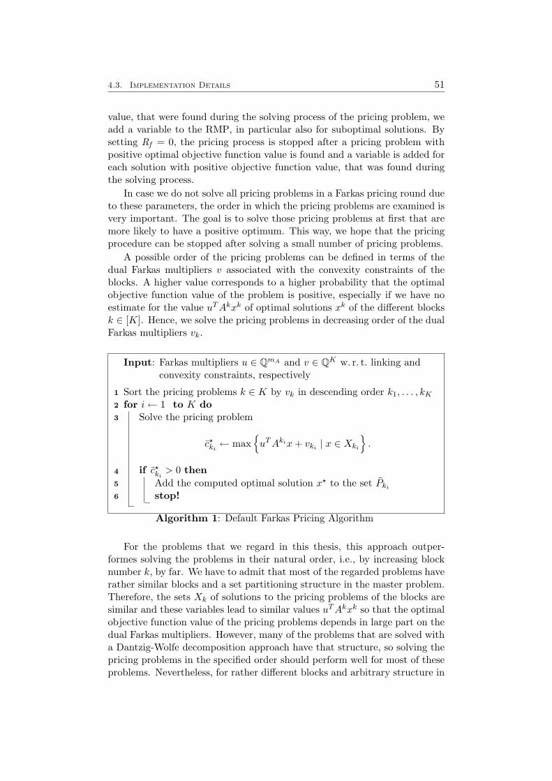
4.3. Implementation Details 51
value, that were found during the solving process of the pricing problem, weadd a variable to the RMP, in particular also for suboptimal solutions. Bysetting Rf = 0, the pricing process is stopped after a pricing problem withpositive optimal objective function value is found and a variable is added foreach solution with positive objective function value, that was found duringthe solving process.
In case we do not solve all pricing problems in a Farkas pricing round dueto these parameters, the order in which the pricing problems are examined isvery important. The goal is to solve those pricing problems at first that aremore likely to have a positive optimum. This way, we hope that the pricingprocedure can be stopped after solving a small number of pricing problems.
A possible order of the pricing problems can be defined in terms of thedual Farkas multipliers v associated with the convexity constraints of theblocks. A higher value corresponds to a higher probability that the optimalobjective function value of the problem is positive, especially if we have noestimate for the value uTAkxk of optimal solutions xk of the different blocksk ∈ [K]. Hence, we solve the pricing problems in decreasing order of the dualFarkas multipliers vk.
Input: Farkas multipliers u ∈ QmA and v ∈ QK w. r. t. linking andconvexity constraints, respectively
Sort the pricing problems k ∈ K by vk in descending order k1, . . . , kK1
for i← 1 to K do2
Solve the pricing problem3
c?ki← max
{uTAkix+ vki
| x ∈ Xki
}.
if c?ki> 0 then4
Add the computed optimal solution x? to the set Pki5
stop!6
Algorithm 1: Default Farkas Pricing Algorithm
For the problems that we regard in this thesis, this approach outper-formes solving the problems in their natural order, i.e., by increasing blocknumber k, by far. We have to admit that most of the regarded problems haverather similar blocks and a set partitioning structure in the master problem.Therefore, the sets Xk of solutions to the pricing problems of the blocks aresimilar and these variables lead to similar values uTAkxk so that the optimalobjective function value of the pricing problems depends in large part on thedual Farkas multipliers. However, many of the problems that are solved witha Dantzig-Wolfe decomposition approach have that structure, so solving thepricing problems in the specified order should perform well for most of theseproblems. Nevertheless, for rather different blocks and arbitrary structure in

52 Chapter 4. Solving the Master Problem
the master problem, defining another order could be more efficient.The default Farkas pricing method is pictured in Algorithm 1. In Sec-
tion 4.4.1, we give a comparison to some other settings.
4.3.2 Reduced Cost Pricing
In the reduced cost pricing routine, we look, from the theoretical point ofview, for a variable of the master problem with the most negative reducedcost. This variable is added to the RMP and the process is iterated. For themaster problem obtained by the Dantzig-Wolfe decomposition, this translatesinto solving the pricing problem (4.9) for each block k ∈ [K]. After that, ifand only if the best optimal objective value is negative, a variable is added tothe RMP that represents the extreme point given by the computed optimalsolution.
By solving all pricing problems, however, we potentially get a whole bunchof variables that can improve the RMP’s current solution, namely for eachpricing problem with negative optimal objective value at least the variablecorresponding to the optimal solution. If we found further (suboptimal) so-lutions with negative objective value during the solving process of the pricingproblems, we could add these variables as well. Note, that in Section 4.1, weadded only one variable to the RMP per pricing round, however, finitenessand correctness of the pricing process are obviously conserved when addingmore than one variable. In this case, the size of the RMP grows faster and werun the risk of creating variables that will never be part of the basis whichleads to a slowdown of the simplex algorithm. We have to trade this offagainst the benefit that variables are created without further effort, whichwould possibly have been created in one of the successive pricing rounds,anyway.
Additionally, when adding only the variable with the most negative re-duced cost, this variable will definitely be chosen to enter the basis, whichequals to the so-called Dantzig pivot rule of the simplex method. Compu-tational experiments (see [32]), however, have shown that this pivot rule ismostly inferior to more sophisticated rules, like steepest-edge pivot rules. Wewill not go into details about pivot rules of the simplex method in this thesisand refer to [85, 32] and the references given there, but we want to give anindication, that adding more than just one variable to the RMP per roundcan help to reduce the number of simplex iterations during the solving pro-cess of the master problem. Since the LP solver is treated as a black box,we do not know which pivot rule is used by it, thus we cannot modify thepricing process to search the variable with the highest priority according tothis pivot rule and add just this variable. However, when adding more thanone variable, the LP solver can choose the “best” of the new variables toenter the basis according to the pivot rule employed by it. Additionally, af-ter performing one simplex iteration, there is the possibility that one of theother newly created variables still has negative reduced cost and can further
4.3. Implementation Details 53
improve the objective function value. This way, we can reduce the numberof times pricing has to be performed and hopefully also the total time spentfor the solving process of the master problem.
Another approach to reduce the effort of the pricing routine is to stopthe pricing process after a given number of variables with negative reducedcosts were found in this pricing round, add these variables to the RMP anditerate the process. That way, we do not solve the pricing problem as statedin Section 4.1, since we do not calculate the most negative reduced cost. Wefind, however, variables with negative reduced cost that can enter the basiswhen the RMP is re-optimized. Finiteness and correctness of the procedureis assured as long as we do not abort the pricing process before finding a newvariable. Thus, at least in the last pricing round, we have to solve all pricingproblems to optimality in order to guarantee that no variable with negativereduced cost exists in the master problem that can improve the solution ofthe RMP.
We included these approaches into our branch-cut-and-price solver GCGand provide some parameters to tune them. In the following, we will namethe most important parameters and their influence.
First of all, let us notice that without imposing limits by parameters, wesolve all pricing problems and add all variables with negative reduced cost tothe RMP that were found in this pricing round. In particular, we also addsuboptimal solutions of the pricing problems as long as they have negativereduced cost.
Since these can be quite a lot of variables, a maximum number Mr ∈ [1,∞]of variables that are added per reduced cost pricing round can be specified.In the default setting, it is set to 100.
In addition to that, we can choose whether the pricing routine is stoppedafter this number of variables with negative reduced cost was found or, al-ternatively, all pricing problems are solved and after that, the Mr variableswith the most negative redced costs are added to the RMP. By choosingthe second possiblity, the parameter is called onlybest, together with a limitMr = 1, we perform pricing as stated in Section 4.1, i.e., we only add onevariable with the most negative reduced cost to the RMP.
Furthermore, we can limit the number of variables created for one blockin a pricing round by a value Mp ∈ [1,∞]. Setting this value to 1 correspondsto taking into account only variables corresponding to an optimal solution ofa pricing problems while a greater value allows to create variables for sub-optimal solutions, too. In the default setting, we set Mp = ∞. Apparently,the parameters Mp and Mr overlap in some cases: By setting Mp ≥ Mr orMp ≤ Mr
K , one of these parameters becomes redundant.Like for the farkas pricing, we introduced a parameter Rr ∈ [0, 1]. It is
a relative limit on the number of pricing problems that are solved in eachpricing round. If the limit is reached and new variables were added in thecurrent pricing round, the round is stopped, otherwise, it is continued untilimproving variables have been found.
54 Chapter 4. Solving the Master Problem
In case we do not solve all of the pricing poblems in each pricing rounddue to the parameter settings, it is also important, in which order the pricingproblems are examined. If we start with solving those pricing problems thatare expected to have the more negative solutions, we avoid solving instancesthat are likely to have a non-negative optimum. The order can be specified bythe parameter sorting . The pricing problems can be solved in their naturalorder, i.e., by increasing k (sorting = 0) or by decreasing dual solution valueof the convexity constraint corresponding to that block (sorting = 1), likeit is also done for the Farkas pricing. This makes use of the fact that foreach block, the negation of the corresponding dual solution value goes intothe reduced costs of the variables corresponding to that block. Hence, thehigher the value, the more likely it is that variables of the block have negativereduced cost. It turned out that like for the Farkas pricing, this ordering ofthe pricing problems is superior, so it is used per default.
Another approach to speed up the pricing process is the use of heuristics.Instead of solving the pricing problems to optimality, we use a heuristicthat is expected to find “good” solutions in a reasonable amount of time.For this purpose, each pricing solver can provide a routine that solves thegiven pricing problem in a heuristic fashion. If a heuristic finds variableswith negative reduced costs, we add them to the RMP, according to thepreviously defined settings. After that, the RMP is resolved and the processis iterated. If the heuristic does not find any variable with negative reducedcost, however, we have to solve the pricing problems to optimality in orderto find an improving variable or to prove that no such variable exists. Theusage of heuristics can be turned on with the parameter useheur , per default,it is disabled.
For the MIP pricing solver, solving the problem heuristically is done bysolving the pricing problem with SCIP, too. In order to limit the effort spentfor the heuristic call of the pricing solver, we limit the number of solving nodesand the number of stalling nodes. The first one is a hard limit on the numberof nodes that are at most processed, the latter defines the number of nodes,that may be processed without finding an improving solution. Additionally,we set a limit on the objective value of solutions, thus only solutions withnegative reduced costs are accepted and we cancel the solving process oncea given gap has been reached.
The reduced cost pricing process is presented in Algorithm 2.
4.3.3 Making Use of Bounds
In Section 4.2, we defined a lower bound LBRMP on the optimal objectivevalue of the master problem that can be computed using the current optimalsolution z?
RMP of the RMP and the optimal solutions c?k, k ∈ [K] of all pricingproblems (see Theorem 4.10). In the following, we describe how we use thisbound to speed up the solving process.

4.3. Implementation Details 55
Input: An optimal dual solution of the RMP π ∈ QmA , ρ ∈ QK
w. r. t. linking and convexity constraints, respectively
nvars← 0 // number of variables added1
heur ← useheur // solve pricing problems heuristically?2
V ← ∅ // set of variables found so far3
Sort the pricing problems k ∈ [K] according to the selected sorting4
method and obtain an order k1, . . . , kK
for i← 1 to K do5
nvarsprob← 0 // nr. of variables found in this problem6
Solve the pricing problem7
c?k ← min{(cki
T − πTAki
)x− ρki
| x ∈ Xki
}(4.12)
heuristically, if heur = TRUE, otherwise, solve it to optimality.if c?ki
< 0 then8
for each solution x? of (4.12) that is found (sorted increasingly9
w. r. t. objective function value) doif(cki
T − πTAki)x? − ρki
< 0 then10
if onlybest then11
V ← V ∪ {(x?, i)}12
nvarsprob← nvarsprob + 113
else14
Pki← Pki
∪ {x?}15
nvars← nvars + 116
nvarsprob← nvarsprob + 117
if nvarsprob = Mp or nvars = Mr then18
break!19
if nvars = Mr or (i ≥ Rr ·K and nvars > 0) then20
break!21
if onlybest then22
Sort the set V w. r. t. the reduced costs of the saved variables23
for (x?, i) ∈ V in increasing order w. r. t. reduced costs do24
Pki← Pki
∪ {x?}25
nvars← nvars + 126
if nvars = Mr then27
break!28
if nvars = 0 and heur = TRUE then29
heur ← FALSE30
Goto Line 531
Algorithm 2: Reduced Cost Pricing Algorithm
56 Chapter 4. Solving the Master Problem
Early branching First, it is possible to define a maximum number ofreduced cost pricing rounds maxrounds ∈ [0,∞] to be performed at eachnode of the branch-and-price tree.
When creating a node, SCIP initially sets its local dual bound to the dualbound of the father node, for the root node, it is set to minus infinity. Thislocal bound is automatically updated once the LP relaxation at the nodeis solved to optimality. If maxrounds < ∞ and this number is exceededfor a branch-and-price node, we do not know whether further variables withnegative reduced cost exist in the master problem. Thus, we did not solvethe master problem to optimality and the RMP’s optimal objective functionvalue is not a valid lower bound for the optimal solution value of the originalprogram.
However, the reduced cost pricing callback of variable pricers in SCIPprovides the possibility to specify a lower bound on the optimal objectivevalue of the local master problem. SCIP then automatically updates thedual bound of the node to this value if it is better, i.e., higher, than itscurrent dual bound. Hence, in each pricing round in which the RMP andall pricing problems are solved to optimality, the pricer computes the lowerbound LBRMP and returns this value so that SCIP updates the dual boundof the node, if possible.
The behavior resulting from setting maxrounds <∞ is denoted by earlybranching in the following, since the solving of the current node is interruptedand branching is performed “earlier”.
We decided to give no possibility to limit the number of Farkas pricingrounds, since then we would not have a feasible solution to the current masterproblem and would not even know whether such a solution exists. On the onehand, if the current master problem is infeasible, proving this by completingthe Farkas pricing process allows us to prune the current node in the branch-and-bound tree. On the other hand, if it is not infeasible, we will have torestore the feasibility in its children, anyway. All the dual rays providingan infeasibility proof at the current node can still proof the infeasibility inthe subsequent nodes, so they have to be forbidden by adding new variablesto the RMP, anyhow. Besides, without knowing a feasible solution of themaster problem, we do not have the guidance for the branching process thatis usually provided by the relaxator’s current solution.
Early branching typically results in a slower increase of the dual bound.In return, the branch-and-price tree is explored faster and nodes that aresituated deeper in the branch-and-price tree are investigated earlier. Sincethese nodes correspond to problems that are more likely to have an integralsolution (e.g., since some variables are fixed to integral values), it may resultin feasible solutions being found earlier in the solving process.
Due to the weaker dual bound, this is primarily useful when we do notwant to solve the problem to optimality, but want to find a solution witha given quality, e.g., a solution that has at most 10% additional cost com-pared to the optimal solution. Besides, this concept is often used for primal

4.3. Implementation Details 57
heuristics. For example, pricing is performed only at the root node. Afterthat, one hopes, that the current set of variables contains a feasible solutionto the extended problem and tries to find a solution quickly by branching ina depth-first-search way (see [10]).
Per default, we set maxrounds =∞ so the number of pricing rounds pernode is not limited.
Early termination Nevertheless, we use a weakened form of early branch-ing, also called early termination of the pricing process (see [97]) even withthe default settings. In case we know that the objective function value of eachfeasible solution is integral—e.g., if the original problem’s objective functioncontains only integer variables with integral coefficients—we stop the pricingprocess if further improvements of the node’s dual bound will never haveany advantages with regard to the bounding process. In the following, wedescribe how this is detected.
Let z?RMP be the optimal objective value of the RMP and LB be the
current dual bound of the active node, i.e., the maximum of the parent node’sdual bound and all feasible lower bounds LBRMP computed in former pricingrounds at the current node. By solving the master problem to optimality,we obtain a lower bound z?
MP on the optimal objective function value of thecurrent original problem. This one lies between the two former values, i.e.,LB ≤ z?
MP ≤ z?RMP (see Section 4.2).
If dLBe ≥ z?RMP then it follows dLBe = dz?
MPe. This means, that the bestfeasible solution for the current problem has objective value at least dLBe, sowe can set the lower bound of the node to dLBe. Solving the master problemto optimality can lead to no better dual bound, thus we can stop the solvingprocess of the master problem. Actually, the dual bound of the node doesnot have to be updated to dLBe as SCIP knows about the integrality of theobjective function value of each solution. Therefore, it prunes the node assoon as a solution with value dLBe or better is found, even if the dual boundLB is maintained.
This result can easily be generalized to problems, for which z ∈ Q existssuch that each feasible solution has value k · z with k ∈ Z: if dLB
z e ≥z?RMPz ,
the solving process of the master at the current node can be stopped.By using early termination, we reduce the so-called tailing-off effect [57].
That means, that the column generation process finds a near optimal solutionin a reasonable amount of time, but obtaining optimality and proving ittypically needs many pricing rounds. Furthermore, the pricing problems oftenget much harder to solve when the dual variables converge to the optimaldual solution of the master problem. The long tail of computations neededto prove the optimality is avoided by stopping the column generation earlier.
However, computing the exact lower bound by solving the master problemto optimality can improve the effectiveness of methods that make use ofso-called pseudocosts. Pseudocosts denote the average increase in the dualbound after tightening the bound of a certain variable (also see Section 5.6.1).

58 Chapter 4. Solving the Master Problem
They are used for example by branching rules [5], node selection strategies [1],and some primal heuristics [11].
Nevertheless, our computational studies (see Chapter 7) show that theeffort saved in the pricing routine compensates this disadvantage and theoverall computation time is decreased when using early termination. How-ever, it can be deactivated with the abortpricing parameter.
Objective limit for LP solving Finally, let us note that the RMP is notalways solved to optimality before the pricing plugin is called. Like moststate-of-the-art MIP solvers, SCIP imposes a limit on the objective functionvalue of the LP. When solving the LP with the dual simplex algorithm,e.g., after adding branching restrictions, the solving process of the LP isstopped as soon as the objective value of the current LP solution is greateror equal to the primal bound. By continuing the solving process of the LP,we would obtain an optimal solution with an objective value not smaller thanthe current objective value of the LP, hence also not smaller than the primalbound. If the LP contains all variables explicitly, i.e., no pricers are active,the current node can be pruned since the current problem cannot containsolutions that are better than the incumbent.
If pricers are active, however, the current LP is just a restricted versionof the implicitly given actual LP. Therefore, by adding more variables tothe restricted LP, we can improve its optimal objective value and will finallyget an optimal solution for the actual LP. This solution can have a betterobjective value than the optimal solution of the restricted LP, hence the nodemust not be pruned. Instead, in order to obtain this optimal solution of theactual LP, pricing has to be performed. If and only if the optimal objectivevalue is then still greater or equal to the primal bound, the node can bepruned.
When the solving process of the LP was stopped due to the objective limit,however, we do not need to solve the restricted LP to optimality. We canuse the current dual solution values, since this solution has to be forbiddenin the dual of the LP in order to obtain a primal LP solution that is betterthan the primal bound. If we find variables with negative reduced costs, weadd them to the LP and iterate the process. If we do not find any variablewith negative reduced cost, then the current dual solution is feasible in thedual of the actual LP and thus, the optimal solution value of the actual LPis greater or equal to the primal bound and the node can be pruned.
4.4 Computational Results
In this section, we describe our experiences of the solving process of themaster problem. We investigate different settings and variants mentioned inthe last section and compare their effectiveness.
We focus on the master problem at the root node and investigate the effort
4.4. Computational Results 59
needed to obtain feasibility of the RMP in Section 4.4.1. In Section 4.4.2, welook at the process of solving the master problem to optimality. However,we do not regard the impact on the performance of the total branch-and-price process. We cannot guarantee that pricing strategies that dominatethe solving process of the master problem at the root node are also superiorfor the branch-and-price process. For example, it could be an advantage tocreate more variables at the root node even if the pricing process at the rootnode takes slightly longer in this case, since the additional variables couldspeed up the solving process of the master problem at subsequent nodes. Onthe other hand, adding much more variables also slows down the simplexalgorithm and it is not clear whether these variables help in finding goodprimal feasible solutions or actually derange this process.
Since the branch-and-bound process and different branching rules werenot yet introduced (this will be done in the next chapter), we will in thefollowing regard several possible pricing strategies and name a subset thatseems to perform well. In Chapter 7, we will then compare some strategieswith respect to the branch-and-price process.
4.4.1 Farkas Pricing
We ran benchmarks to compare the performance of the default Farkas pricingsettings (see Algorithm 1) with the following variations.
• “All vars”: all pricing problems are solved in each pricing round andall variables are added to the RMP that cut off the dual ray, i.e., fulfillcondition (4.10). This corresponds to Mf =∞.
• “No sort.”: like in the default setting, just one variable is added to theRMP per pricing round, but the pricing problems are not sorted w. r. t.the dual Farkas multipliers v, instead they are solved in their naturalorder.
• “2 vars”: the pricing problems are sorted as for the default settings,but instead of adding just the first variable, we add up to two variables.With this setting, we want to investigate, whether adding not just one,but also not all variables found is a good idea. This corresponds toMf = 2.
• “2%”: the pricing problems are sorted as for the default settings, butinstead of adding just the first variable, we solve 2% of the pricingproblems. The pricing round is stopped, if variables were added so far,otherwise, it is continued until the first variable is added. We obtainthis behavior for Mf =∞ and Rf = 0.02.
• “1 prob”: the pricing problems are sorted as for the default settings,but instead of adding just the best solution of a pricing problem, weadd all solutions of the problem that have a positive objective function
60 Chapter 4. Solving the Master Problem
value. As soon as a pricing problem gave rise to new variables, thepricing round is stopped. This corresponds to Mf =∞ and Rf = 0.
Table 4.1 summarizes the results, further details can be found in Ta-bles D.1 to D.10 in Appendix D. The computational environment and thetest sets are described in Section 3.3.
The upper and middle part of Table 4.1 picture the number of pricingrounds and solved pricing problems, respectively, the lower part the time thatwas needed to achieve feasibility of the RMP at the root node. We excludedthe time needed for presolving, problem creation, primal heuristics etc. andlist only the sum of pricing and LP solving time. The solving process wasstopped after at most 5 minutes.
The first column shows—in absolute numbers—for each test set the shif-ted geometric mean of these values when performing Farkas pricing withdefault settings. The columns “all vars”, “no sort.”, “2 vars”, “2%”, and“1 prob”, show the percental change in the shifted geometric mean for thevariations compared to the default settings.
We used the convexification approach for these computations so the iden-tical blocks in the vertex coloring and the bin packing problem where treatedindependently. Hence, for these problems, all pricing problems have equiva-lent optimal solutions, so the pricing problems with greater Farkas multipli-ers have better optimal objective values. The same holds for the capacitatedp-median problem (CPMP): The only difference between the blocks is the ob-jective function, which is disregarded for the Farkas pricing. For the resourceallocation problems, obtaining feasibility is rather easy since setting all vari-ables to zero in the original problem gives us a feasible solution. Therefore,for each of the pricing problems, the zero solution has to be found and thecorresponding variable has to be added to the RMP in order to restore fea-sibility. Nevertheless, the presented results give us some indication for theimpact of the different settings.
For the default settings (column “default”), we solved exactly one pricingproblem per round, which was to be expected due to the similar structure ofthe pricing problems.
When adding all variables (column “all vars”), the shifted geometric meanof the number of pricing rounds is decreased by 68%. This was to be expectedsince we add more variables in each round, in particular, in each round wealso add the variable that would be added when performing this pricing roundwith default settings. The additional variables potentially cut off other dualrays that would have caused an infeasibility in a subsequent iteration. Inreturn, we have to solve all pricing problems in each pricing round, hence wesolve about sixteen times as many pricing problems in spite of the consid-erably smaller number of pricing rounds. Because of this, the total runningtime increased more than sevenfold.
When not sorting the pricing problems (column “no sort.”), the numberof pricing rounds, the number of pricing problems that are solved, and the

4.4. Computational Results 61
test set default all vars no sort. two vars 2 % 1 prob
roun
ds
cpmp50s 238.4 −60 +763 −25 −32 −32cpmp100s 571.3 −67 +1038 −30 −49 −41cpmp150s 1011.4 −77 +424 −35 −57 −48cpmp200s 1457.7 −82 +126 −38 −60 −52coloring 241.1 −40 +829 −10 −8 −4rap32s 37.7 0 0 0 0 0rap64s 19.0 0 0 0 0 0bindata1-n1s 227.3 −73 +771 −24 −11 −4bindata1-n2s 545.6 −78 +684 −24 −37 −15bindata1-n3s 1463.0 −84 +237 −24 −56 −8mean 385.4 −68 +353 −23 −38 −25
prob
lem
s
cpmp50s 238.4 +1895 +1938 +773 −32 −32cpmp100s 571.3 +3209 +3453 +1215 +3 −41cpmp150s 1011.4 +3428 +2315 +1553 +30 −48cpmp200s 1457.7 +3563 +1831 +1880 +60 −52coloring 241.1 +1251 +1444 +163 +9 −4rap32s 37.7 +3444 +1744 +3444 +23 0rap64s 19.0 +1721 +885 +1721 0 0bindata1-n1s 227.3 +906 +6052 +319 −3 −4bindata1-n2s 545.6 +1517 +5372 +505 +27 −15bindata1-n3s 1463.0 +2273 +1618 +809 +57 −8mean 385.4 +1690 +1849 +745 +16 −25
tim
e
cpmp50s 0.5 +891 +2603 +76 −30 −31cpmp100s 3.6 +4964 +7982 +95 −40 −58cpmp150s 15.2 +1964 +1854 +52 −31 −62cpmp200s 50.7 +501 +481 +21 −26 −72coloring 3.9 +903 +5294 +117 +10 −3rap32s 0.1 +193 +99 +194 +2 +1rap64s 0.0 +79 +40 +80 0 0bindata1-n1s 0.2 +151 +10832 +40 −1 +1bindata1-n2s 1.1 +852 +27542 +177 −14 −23bindata1-n3s 8.5 +701 +3315 +134 −31 −1mean 5.2 +602 +1857 +63 −21 −44
Table 4.1. Performance effect of different variants of the Farkas pricing for obtainingfeasibility of the RMP at the root node. The first column denotes the shifted geometricmeans of the number of pricing rounds (top), the number of pricing problems that weresolved (middle) and the master problem solving time in second (bottom) for the defaultsettings. The other columns denote the percental changes in the shifted geometric mean ofthe values for the other settings. Positive values represent a deterioration, negative valuesan improvement.

62 Chapter 4. Solving the Master Problem
solving time of the master problem are increased by far. The increase of thenumber of pricing problems is consequential, since for the default settings, thepricing problem that is solved first has the best solutions due to the structureof the problems in our test set. Hence, we only solve one pricing problemper pricing round for the default settings. When not sorting the pricingproblems, it can happen that we need to solve several pricing problems untilwe find a solution with positive objective function value. However, also thenumber of pricing rounds is more than quadrupled. This can be explained bythe fact, that we add a variable with negative objective value in its pricingproblem, but there also exists an equivalent variable in the pricing problemwith the highest corresponding Farkas multiplier, which thus has a betterobjective function value and which is added in the default settings. Thisshows, that also for the Farkas pricing, adding variables that have a betterobjective function value in the pricing problem reduces the number of pricingrounds by far. A motivation for this is that a variable with better objectivevalue in its pricing problem corresponds to a potentially tighter constraintin the dual of the RMP, at least, it only allows smaller multiples of the raygiven by the dual Farkas multipliers than a solution with smaller objectivefunction value.
Adding at most a given number of variables in each pricing round—we tried adding two variables in each round (column “two vars”)—helps indecreasing the number of pricing rounds, but it has an essential drawback: Ifthere only exists one variable that fulfills condition (4.10), we have to solveall the pricing problems. This results in an eightfold increase of the numberof pricing problems that are solved, although the number of pricing roundsis decreased by 23% in the shifted geometric mean. Therefore, the shiftedgeometric mean of the total time is increased by 63%, too.
In order to overcome this drawback, we limit the number of pricing prob-lems that are solved and not the number of variables added. Column “2%”shows the results for solving 2% of the pricing problems and adding all vari-ables that are found during this process. If no variable was found so far,we continue the pricing round until variables are added, otherwise, we stopthe pricing round. This way, we obtain a decrease in the shifted geometricmean of the number of pricing rounds of 38% with a moderate increase ofonly 16% in the number of pricing problems that are solved. The shiftedgeometric mean of the total time is even decreased by 21%.
Finally, we tried to add all variables of a pricing problem instead of onlythe first one (column “one prob”). This way, we still solve just one pricingproblem per pricing round, but we add more variables and thus, we canreduce the number of pricing rounds by 25% and the total time by 44%.Hence, this variant seems to be superior to the default settings.
Finally, let us note that adding two variables led to one timeout, addingall variables resulted in 38 timeouts and without sorting the pricing problems,the time limit was reached by 95 out of 198 instances, so the results for thesesettings would have been even worse without imposing a time limit.

4.4. Computational Results 63
We draw the following conclusions that are valid at least for our test sets:
• Adding better variables, i.e., variables with higher objective functionvalue in the pricing problems, significantly reduces the number of pric-ing rounds and the number of pricing problems that are solved as wellas the total time.
• Although one variables suffices to cut of the dual ray, adding morevariables per pricing round typically reduces the number of pricingrounds.
• However, a fixed limit greater than one—also infinity—of variables toadd typically increases the number of pricing problems, that are solvedand also the total time, since all problems have to be solved if thisnumber is not exceeded. Imposing a limit on the number of pricingproblems is therefore superior.
Aggregating blocks in the discretization approach
Until now, we only investigated the Farkas pricing strategies for the convexi-fication approach. In the following, we give a comparison between convexifi-cation and discretization approach. When not aggregating blocks, the pricingprocess is exactly the same for both approaches. Hence, we only investigatethe vertex coloring and the bin packing instances in this subsection, for whichblocks are identical and can thus be aggregated. In Table 4.2, we picture thenumber of pricing rounds, the number of pricing problems that are solvedand the solving time of the master problem for setting “1 prob”, which out-performed the default settings for the convexification approach. Since weonly have one pricing problem in the discretization approach, we do not havethe variety of possible pricing strategies as in the convexification approach.We solve one—the only—pricing problem. We tried two possibilities of howmany variables are added. On the one hand, we can add to the RMP justone variable corresponding to an optimal solution. This is done in setting“disc best”. On the other hand, we can also add all variables correspondingto solutions with positive objective function value that were found duringthe solving process of the pricing problem. The results for this approach arelisted in column “disc all”.
Setting “disc all” resembles “1 prob” for the convexification approach,where we solve the pricing problem with the most positive dual Farkas mul-tiplier and add all variables corresponding to solutions with positive objectivefunction value, afterwards. Although this sounds similar, setting “disc all” issuperior in terms of pricing rounds, pricing problems that are solved and totaltime needed for Farkas pricing at the root node. In the convexification ap-proach, it may happen that a variable representing a point was created in oneof the blocks, but a variable corresponding to the same point will be neededin another block later on. Then, in another pricing round, this variable has

64 Chapter 4. Solving the Master Problem
test set 1 prob disc all disc bestro
unds
coloring 232.4 −26 −24bindata1-n1s 219.1 −72 −71bindata1-n2s 462.1 −74 −72bindata1-n3s 1352.8 −83 −81mean 442.5 −69 −67
prob
lem
s
coloring 232.4 −26 −24bindata1-n1s 219.1 −72 −71bindata1-n2s 462.1 −74 −72bindata1-n3s 1352.8 −83 −81mean 442.5 −69 −67
tim
e
coloring 3.7 −24 −20bindata1-n1s 0.2 −15 −14bindata1-n2s 0.8 −73 −64bindata1-n3s 8.4 −95 −91mean 2.9 −73 −68
Table 4.2. Performance effect of the discretization approach for obtaining feasibility ofthe RMP at the root node. The first column denotes the shifted geometric means of thenumber of pricing rounds (top), the number of pricing problems that were solved (middle)and the runtime (bottom) for the convexification approach with setting “1 prob”, The nextcolumns denote the percental change in the geometric mean of these values when using thediscretization approach and adding only the best variable (second column) or all variablesthat cut off the dual ray (third column). Positive values represent a deterioration, negativevalues an improvement.
to be created, too. This cannot happen in the discretization approach withaggregated blocks since we do not distinguish the blocks and only have onepricing problem. In some sense, the pricing in the discretization approachis similar to pricing in the convexification approach, thereby adding not justvariables for one block, but the equivalent variables for all the other blocks,too. However, this leads to a much bigger RMP slowing down the simplexmethod and also the number of constraints in the RMP is slightly smaller forthe discretization approach since we have just one convexity constraint.
Like for the convexification approach, adding just one variable per roundis inferior to adding all variables with positive objective function value of oneproblem (which this time is the only one). Thus, we should think aboutchanging the default setting from adding just one variable to adding allvariables of one problem with positive objective function value for both ap-proaches. However, we do not know whether adding all variables is alsosuperior w. r. t. the branch-and-price process. We performed computationsabout this and answer this question in Section 7.1.
To sum up, the discretization approach outperforms the convexificationapproach in the case of identical blocks as it was to be expected. Especiallyfor test sets bindata1-n2s and bindata1-n3s, where each instance has 100
4.4. Computational Results 65
and 200 identical blocks, respectively, feasibility of the RMP is obtainedabout four and twenty times faster, respectively.
4.4.2 Reduced Cost Pricing
In this subsection, we present some computational results for the reducedcost pricing. We just list the effort of the reduced cost pricing process of themaster problem at the root node, so we excluded the effort for the Farkaspricing process. Furthermore, for the time listed in the tables, we also elimi-nated the time needed for presolving, problem creation, primal heuristics etc.and list only the time needed for the solving process of the master problem,i.e., the sum of pricing and LP solving time. We imposed a time limit of fiveminutes for each instance, except for the resource allocation problems wherewe set a time limit of thirty minutes as the solving process of the masterproblem takes much longer for these instances.
Again, we start with a comparison of some fundamental strategies. Thedefault pricing routine adds at most 100 variables to the RMP in each pricinground (Mr = 100). The pricing process is stopped after this number ofvariables was added, so we set onlybest = FALSE . We do neither limit thenumber of variables created per pricing problem (Mp =∞) nor the number ofpricing problems that are solved in a single pricing round (Rr = 1). Table 4.3summarizes the results of the computations. More details can be found inTables D.11 to D.20.
A first observation is the considerably smaller number of pricing roundsfor the default settings compared to Farkas pricing, which corresponds inparts to the fact that we add much more variables in each pricing round.In the shifted geometric mean, about 30 pricing problems are solved in eachpricing round and the time needed for reduced cost pricing is about six timeshigher than the time needed for Farkas pricing. This shows, that the reducedcost pricing is much more important than the Farkas pricing for the overallperformance. This holds even more for the branch-and-price process since atthe subsequent nodes, we start with the set of variables that were createdbefore so we have to perform just a few—if any—Farkas pricing rounds torepair an infeasibility caused by the branching restrictions.
Pricing strategy “only best” solves all pricing problems and adds the vari-able with the most negative reduced cost. This corresponds to the pricingprocess as we described it from the theoretical point of view in Section 4.2.We set Mr = 1 and onlybest = TRUE . This pricing method does not per-form well: The number of pricing rounds, the number of pricing problemsthat are solved and the time needed for reduced cost pricing are increasedby far. Actually, the values would have been even worse if we had not im-posed a time limit: 101 out of 198 instances hit the time limit and were thusstopped before the master problem was solved to optimality. This is alsothe explanation for the decrease of the number of pricing rounds for test setbindata1-n3s. As conjectured in Section 4.3.2, adding more than just the

66 Chapter 4. Solving the Master Problem
test set default only best all vars 100best one prob
roun
ds
cpmp50s 21.7 +1319 −15 +3 +2245cpmp100s 35.8 +1761 −34 +5 +2890cpmp150s 51.3 +662 −46 +5 +2979cpmp200s 69.6 +118 −55 −4 +2160coloring 40.5 +12 −21 −22 +21rap32s 48.4 +332 −63 −51 +602rap64s 35.3 +190 −56 −45 +324bindata1-n1s 34.2 +55 +5 +7 +7bindata1-n2s 79.1 +64 −2 +18 −6bindata1-n3s 132.6 −19 −26 −14 −14mean 52.2 +237 −32 −10 +511
prob
lem
s
cpmp50s 753.3 +1916 +20 +42 +333cpmp100s 1539.0 +4214 +51 +136 +712cpmp150s 2515.1 +2210 +62 +212 +671cpmp200s 3534.6 +729 +73 +273 +402coloring 487.3 +71 +24 +24 −83rap32s 792.2 +831 −14 +12 +390rap64s 321.9 +453 −6 +14 +159bindata1-n1s 937.4 +77 +22 +25 −92bindata1-n2s 3370.1 +166 +55 +89 −95bindata1-n3s 6902.7 +128 +98 +142 −96mean 1438.0 +551 +35 +81 +9
tim
e
cpmp50s 1.9 +1548 +27 +49 +462cpmp100s 4.5 +3608 +84 +159 +788cpmp150s 9.3 +2920 +112 +237 +799cpmp200s 16.5 +1270 +129 +281 +622coloring 34.1 +52 +23 +21 −82rap32s 178.0 +684 −16 +4 +427rap64s 289.7 +342 −10 +7 +198bindata1-n1s 6.8 +149 +25 +25 −90bindata1-n2s 51.1 +190 +64 +82 −88bindata1-n3s 106.7 +160 +138 +127 −90mean 33.8 +438 +37 +62 +47
Table 4.3. Performance effect of different variants of reduced cost pricing for solving themaster problem to optimality at the root node. We list the shifted geometric means of thenumber of pricing rounds (top), the number of pricing problems that were solved (middle)and the runtime (bottom) for reduced cost pricing with default settings (first column).The other columns denote the percental changes in the shifted geometric mean of thesevalues for the other settings. Positive values represent a deterioration, negative values animprovement.

4.4. Computational Results 67
variable with the most negative reduced cost speeds up the solving processby far.
Strategy “all vars” is the opposite: We solve all pricing problems and addall variables to the RMP that are found during the solving process and thathave negative reduced costs. Therfor, we set Mr =∞, Mp =∞, and do notlimit the number of pricing problems that are solved in each pricing round(Rr = 1). As for the Farkas pricing, this typically reduces the number ofpricing rounds compared to the default setting, since more variables are addedin each round. The number of pricing problems that are solved increases andso does the total time. However, for the sets of RAP instances, this settingperformes better than the default setting. We will give an interpretation forthis later, but it already shows, that there is a big variation on the reducedcost pricing performance for the different test sets.
We also tested whether adding not the first 100 variables that are found,but the 100 variables with the most negative reduced costs improves theperformance (column “100best”). The only difference to the default settingsis that we set onlybest = TRUE . This increases the number of pricingproblems that are solved, since we have to solve all pricing problems in orderto determine the 100 “best” variables. Hence, also the total time is increasedby about 50%.
Finally, for pricing strategy “one prob”, we perform the reduced costpricing similar to the best setting for the Farkas pricing: We stop the pricinground as soon as a pricing problem has a negative optimal objective valueand add all variables with negative reduced costs that were found during thesolving process of this problem. The shifted geometric mean of the numberof pricing rounds is increased by far, as it was to be expected since we adda smaller number of variables in each pricing round. This pricing methodperforms very well for the vertex coloring and the bin packing instances. Inreturn, for the other instances, it performs badly.
We can see that due to the rather different structure of the problemclasses, we get different results for the pricing methods that we investigate.This shows that the performance of a pricing strategy is always problem de-pendent and there does not exist a dominating pricing method. However, wecan draw some conclusions based on the presented computational results. Forthe vertex coloring and the bin packing instances, pricing strategy “one prob”performs best. This can be explained by the identical blocks: As all problemsare identical and only the dual solution values of the corresponding convexityconstraints differ, the pricing problems are rather similar. Therefore, also thesolutions that are found during the solution process of the pricing problemsare also rather similar. Thus, spending more effort to solve more than onepricing problem leads to equivalent variables corresponding to other blocksthat just slow down the simplex algorithm.
For the class of resource allocation problems, adding all the variablesthat are found and which have negative reduced cost in each pricing roundseems to perform best and adding the 100 best variables is competitive to the
68 Chapter 4. Solving the Master Problem
default settings. These problems have rather different blocks. Each block hasthe same structure, i.e., it consists of a number of capacity constraints, butthe variables corresponding to the blocks are different, they have arbitraryobjective function values and different coefficients in the constraints of themaster problem. Hence, optimal solutions to different blocks are independentand differ in the master problem’s coefficients, so each variable is importantand can help during the solving process.
In contrast to that, for the capacitated p-median instances, the blocksare distinct, but still related. Each solution to a pricing problem is alsovalid for all other pricing problems and the corresponding variables havethe same coefficients in the constraints of the master problem, they onlydiffer in terms of the objective function coefficients. Therefore, adding morevariables to the RMP in each round than just a few helps since it allowsmore sophisticated pivot rules in the simplex method and multiple simplexsteps after one pricing round. Nevertheless, since the variables are somehowsimilar, adding all variables leads to many similar variables out of which onlya few can be used, so it does not pay off.
Aggregating blocks in the discretization approach
Again, we investigate the effect of the discretization approach on the per-formance. We only regard the problems that have identical blocks in thefollowing, since for the other problems, the pricing process is the same forconvexification and discretization approach. For the regarded problems, pric-ing strategy “one prob” performed best for the convexification approach: Themaster problem was solved five to ten times faster with it than with the de-fault settings. Therefore, we take the performance for this strategy as thereference value and compare it to the discretization approach in Table 4.4.More details can be looked up in Tables D.5 and D.8 to D.10. In particular,we regard two different strategies for the pricing routine: “disc all”, where weadd all variables to the RMP that were found during the pricing process andthat have negative reduced costs and “disc best”, where only one variablewith the most negative reduced cost is added to the RMP.
The first observation is that the number of pricing rounds needed for re-duced cost pricing is higher for the discretization approach. However, thisis not an attribute of the reduced cost pricing routines, but it arises fromthe different Farkas pricing methods used for the convexification and thediscretization approach. The default Farkas pricing method for the convex-ification approach takes longer than its counterpart for the discretizationapproach, but it also creates more variables. Due to the smaller number ofvariables contained in the RMP at the beginning of the reduced cost pricingprocess, more variables are created afterwards for the discretization approachand so the number of pricing rounds is higher, too.
However, the number of pricing problems that are solved in the reducedcost pricing process is slightly reduced when using the discretization ap-
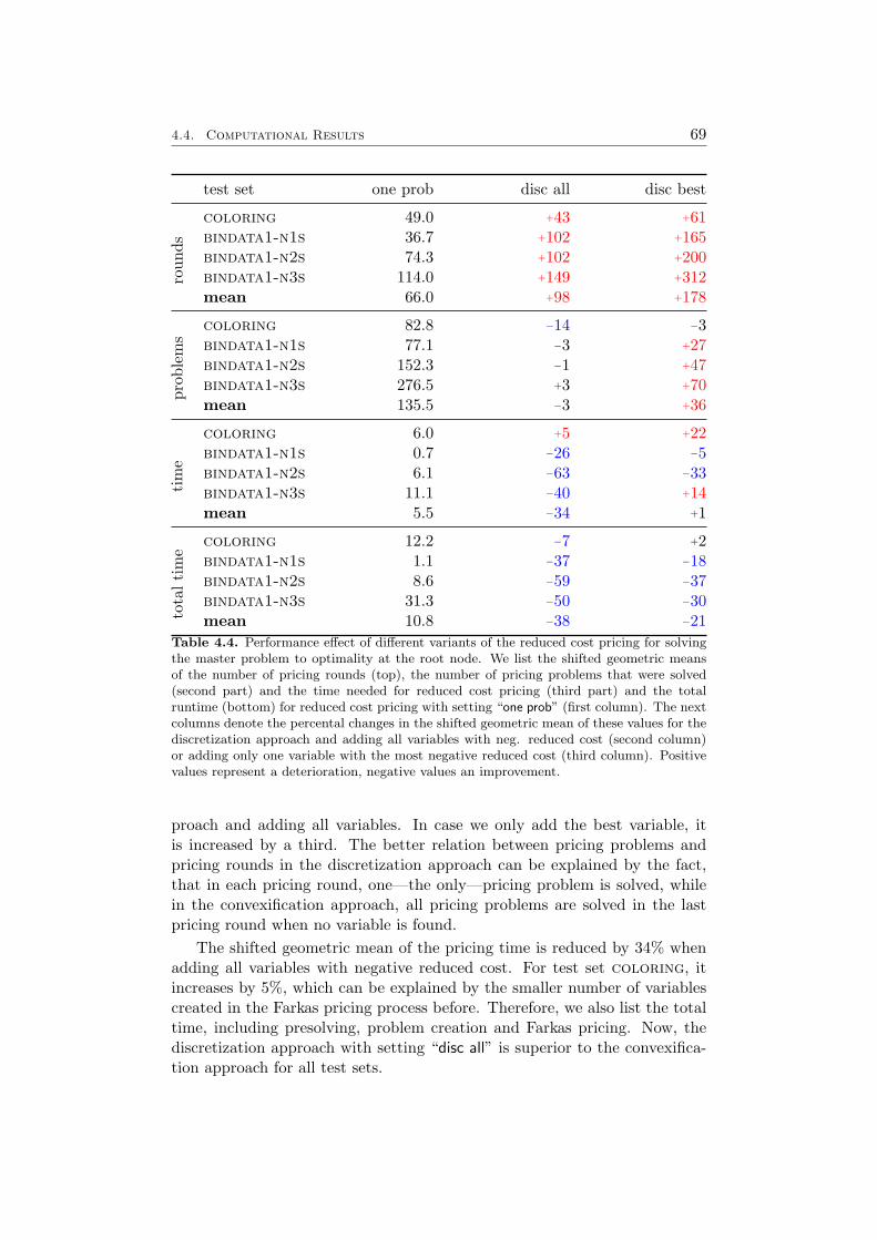
4.4. Computational Results 69
test set one prob disc all disc bestro
unds
coloring 49.0 +43 +61bindata1-n1s 36.7 +102 +165bindata1-n2s 74.3 +102 +200bindata1-n3s 114.0 +149 +312mean 66.0 +98 +178
prob
lem
s
coloring 82.8 −14 −3bindata1-n1s 77.1 −3 +27bindata1-n2s 152.3 −1 +47bindata1-n3s 276.5 +3 +70mean 135.5 −3 +36
tim
e
coloring 6.0 +5 +22bindata1-n1s 0.7 −26 −5bindata1-n2s 6.1 −63 −33bindata1-n3s 11.1 −40 +14mean 5.5 −34 +1
tota
lti
me
coloring 12.2 −7 +2bindata1-n1s 1.1 −37 −18bindata1-n2s 8.6 −59 −37bindata1-n3s 31.3 −50 −30mean 10.8 −38 −21
Table 4.4. Performance effect of different variants of the reduced cost pricing for solvingthe master problem to optimality at the root node. We list the shifted geometric meansof the number of pricing rounds (top), the number of pricing problems that were solved(second part) and the time needed for reduced cost pricing (third part) and the totalruntime (bottom) for reduced cost pricing with setting “one prob” (first column). The nextcolumns denote the percental changes in the shifted geometric mean of these values for thediscretization approach and adding all variables with neg. reduced cost (second column)or adding only one variable with the most negative reduced cost (third column). Positivevalues represent a deterioration, negative values an improvement.
proach and adding all variables. In case we only add the best variable, itis increased by a third. The better relation between pricing problems andpricing rounds in the discretization approach can be explained by the fact,that in each pricing round, one—the only—pricing problem is solved, whilein the convexification approach, all pricing problems are solved in the lastpricing round when no variable is found.
The shifted geometric mean of the pricing time is reduced by 34% whenadding all variables with negative reduced cost. For test set coloring, itincreases by 5%, which can be explained by the smaller number of variablescreated in the Farkas pricing process before. Therefore, we also list the totaltime, including presolving, problem creation and Farkas pricing. Now, thediscretization approach with setting “disc all” is superior to the convexifica-tion approach for all test sets.

70 Chapter 4. Solving the Master Problem
Setting “disc best” performs better than the convexification approach,too, but it is inferior to setting “disc all”. Hence, it pays off to add morevariables with negative reduced costs than just the “best” one, also for thediscretization approach. Since solving the pricing problems consumes mostof the time needed for pricing, we should therefore add all variables withnegative reduced costs to the RMP that are found during the pricing process,hoping that this reduces the number of pricing rounds and thus also thenumber of pricing problems that need to be solved.

Chapter 5
Branching
In Chapter 4, we have described how we can solve the master problem toget a lower bound on the optimal objective value of the original problem(Model 2.1). The optimal solution to the master problem that is computedthis way fulfills all constraints in the extended problem, except for the inte-grality restrictions. Transferring this solution to the original variable spacegives rise to a solution of the original problem that does not neccessarily ful-fill the integrality restrictions (2.4), but all the other constraints contained inthe original problem. If it additionally fulfills the integrality restrictions, wehave solved the original problem to optimality. Otherwise, we use a branch-and-bound process to obtain integrality.
The special thing about branch-and-bound in our approach is the fact,that we do not solve one problem, but two equivalent problems simultane-ously: the original problem and the extended problem. This can be inter-preted in two ways, as we explain in the following.
Let us start, however, with the connection between integrality in the orig-inal problem and integrality in the extended problem. For the convexificationapproach, the connection is clear. Since the integrality in the extended prob-lem is defined in terms of the original variables, a solution to the extendedproblem is integral if and only if its counterpart for the original problem isso, too. Therefore, when using the convexification approach, it is natural toperform branching in terms of the original variables, but this is also possiblefor the discretization approach. How branching can be performed in terms ofthe original variables and how the branching decisions influence the extendedformulation is described in Section 5.1.
This leads us to the first interpretation of the branch-and-bound solvingprocess: what we do is solving the original problem with a branch-and-boundmethod. In contrast to the LP-based branch-and-bound algorithm used bymost state-of-the-art MIP solvers like Cplex, Gurobi, CBC or SCIP, we donot solve the standard LP relaxation of the original problem at each nodeof the branch-and-bound tree. In order to compute a lower bound and asolution that fulfills all but the integrality constraints, we use the Dantzig-Wolfe decomposition at each node. We reformulate the current problem,
71

72 Chapter 5. Branching
obtain a master problem that is then solved and that provides a lower boundfor that node. The solution of the master problem can then be transferredto a solution of the original problem that does not neccessarily fulfill theintegrality restrictions. It can be used in the same way as the LP solution:It is checked for integrality and guides the branching decisions. We can say,we replaced the LP relaxation by a special relaxation that solves the masterproblem.
For the discretization approach, however, we also obtain integrality ofthe original solution by enforcing integrality of the solution to the masterproblem. Hence, we can in this case also perform branching in terms ofthe variables of the master problem. Branching rules that work in this wayare presented in Sections 5.2, 5.4 and 5.5. In fact, we do not need do con-sider the original problem anymore during the solving process, we just solvethe extended problem to optimality and transfer the optimal solution of theextended problem to an optimal solution of the original problem.
This is the second interpretation: at the beginning of the solving process,we transform the original problem into an equivalent problem, the extendedproblem. This problem is solved with a branch-and-price approach, the com-puted optimal solution is then retransformed into the original variable spaceand gives us an optimal solution to the original problem. Strictly speak-ing, one could say that we only reformulated the problem and solved thisreformulation.
It is not possible to draw a distinct line between the two interpreta-tions, since most branching decision can be expressed in both formulations.Branching decisions in the original problem have to be expressed in terms ofthe variables of the extended problem and added to it. This must be doneto assure that the master problem gives rise to an original solution that ful-fills all but the integrality constraints, thus in particular also the branchingrestrictions. Nevertheless, most of the branching decisions are derived fromeither the original or the master problem and then transfered to the otherproblem. Hence, they typically have the more natural expression in one ofthe problems.
However, we will still consider the original problem, even if we derive thebranching decisions from the extended problem and use the additional infor-mation provided by the original problem to speed up the solving process. Forexample, we do not always need to solve the extended problem to optimality.Since our prior target is to solve the original problem to optimality, we donot insist on achieving an optimal solution to the extended formulation. Asfractional solutions to the extended problem can lead to an integral solu-tion of the original problem—a nontrivial combination of extreme points canfor instance represent an interior point xk ∈ Xk like in the convexificationapproach—we consider a problem to be solved once the solution to the mas-ter problem transfers to an integral solution of the original problem, even ifthe master solution is not integral itself.
Finally, let us clarify, that the variables added to the RMP at the root

5.1. Branching on Original Variables 73
node do not suffice for the further solution process. In order to solve themaster problem of a node, we always have to perform pricing and add vari-ables to the RMP that can improve the current solution or fix an infeasibilityarising from the branching restrictions.
5.1 Branching on Original Variables
As described above, the solving method can be interpreted as a branch-and-bound process on the original formulation that uses the master problem as arelaxation rather than the standard LP relaxation. In this context, it wouldbe natural to perform branching in terms of the original variables. Moststate-of-the-art MIP solvers use a branching on variables in the branch-and-bound process, e.g., most infeasible branching, pseudocost branching, strongbranching, or reliability branching (see [5]). In this section, we describe howbranching on variables of the original problem can be transferred to theDantzig-Wolfe decomposition approach presented in this thesis. This branch-ing scheme is widely proposed in the lierature, see for instance [47, 10, 29].
We start with the application to the convexification approach, since thisis the natural branching scheme for this approach. After that, we describehow this branching scheme can be used in the discretization approach, too.
After solving the master problem to optimality, we get a solution x of theoriginal problem according to the coupling constraints (2.13). The integralityrestrictions in the extended problem are expressed in terms of the originalvariables, so if they are fulfilled, x is an optimal solution of the currentoriginal problem and we do not need to perform branching at the currentnode. Otherwise, there exists a variable xk
i , k ∈ [K], i ∈ [n?k] of the original
problem with fractional value xki .
Branching on this variable means creating two children, one with an ad-ditional constraint
xki ≤ bxk
i c (5.1)
which we call the down-branch, and the up-branch with the additional con-straint
xki ≥ dxk
i e. (5.2)
Ways to Enforce the Branching Decision
We have two possibilities, where to add the branching constraints (5.1)and (5.2) in the down-branch and up-branch, respectively. As a branchingconstraint contains variables of just one block, namely exactly one variablexk
i , we can add it to the structural constraints (2.2) of this block. On theother hand, we can also interpret the branching constraint as a part of thelinking constraints (2.1) and add it to this part of the constraints.
74 Chapter 5. Branching
In both cases, we get a modified original problem corresponding to thenewly created child node. We can again apply the Dantzig-Wolfe decompo-sition for MIPs on this problem, like described in Chapter 2, in order to getan extended formulation as well as a master problem that both consider thebranching decision. In fact, we do not need to do the reformulation fromscratch, we can adapt the current extended formulation and master problemto the new original problem.
In the following, we describe how this can be done and which effect it hason the pricing subproblems. We do this on the example of the up-branch,the down-branch is handled similar.
Adding Branching Constraints to the Linking Constraints On theone hand, we can add the branching constraint (5.2) to the linking con-straints (2.1). Hence, we get an additional constraint∑
p∈Pk
piλkp +
∑r∈Rk
riλkr ≥ dxk
i e
in the extended formulation and the master problem. For this constraint, weget an additional dual variable σ which has to be respected in the pricingroutine. It is simply subtracted from the objective value of xk
i in the pricingproblem so that the pricing problem changes to the following:
c?k = min{(ck
T − πTAk − eiσ)x− ρk | x ∈ Xk
}.
Thus, the reduced costs of the potential variables change, but any methodthat was used before to solve the pricing problems can still be used since thestructure of the problem stays the same. The sets of variables correspondingto each block stay the same, in particular, all variables that we created sofar are still valid.
Adding Branching Constraints to the Structural Constraints Onthe other hand, if we add the branching constraint (5.2) to the structural con-straints (2.2), the set Xk is changed and so are the sets Pk and Rk of variablesfor this block. In the pricing subproblem for block k, the constraint (5.2) isadded. When the pricing problems are solved by a MIP solver, this con-straint can be handled easily, but if we solve the pricing problems with aspecial purpose solver, this solver has to be able to take into account upperand lower bounds on the variables. This is, however, the case in most of theapplications: In the bin packing problem or the capacitated p-median prob-lem, where the pricing problem is a knapsack problem, we remove items inthe preprocessing, that have a fixed value and subtract the sizes of the itemsthat have value fixed to 1 from the total capacity. For the vertex coloringproblem, the pricing problem is a stable set. Forcing a node to be part ofthe stable set corresponds to removing all nodes from the problem that are

5.1. Branching on Original Variables 75
adjacent to it. If a variable is fixed to 0, the corresponding node can simplybe removed.
In addition to that, we have to make sure, that we only use variablescorresponding to points and rays that fulfill the branching constraint. If wedo not start with an empty set of variables at each node, but use variablesthat were created before at other nodes, we have to check these variables fortheir feasibility w. r. t. the new pricing problem. If they do not fulfill the newconstraint, they are not allowed to be used in any solution of the master LPat the current node and thus, they have to be removed or forbidden for thecurrent node.
Except for the modified sets Pk and Rk, the extended formulation and themaster problem stay the same, in particular, the number of constraints staysthe same, so we have the same dual variables as before and the calculation ofthe objective function coefficients of the variables in the pricing subproblemsdoes not change.
Comparison Adding the constraints to the structural constraints usuallyresults in a tighter lower bound than adding it to the linking constraints, sincethe latter only cuts off points that do not satisfy the new constraint whilethe former also forbids points that fulfill the constraint but do no longer liein the convex hull of the points that fulfill both the structural constraints—including the new one—as well as the integrality restrictions.
The better lower bound is achieved at the cost of a changed structureof the subproblem, possibly preventing the usage of a special purpose solverand the effort that has to be spent to assure the feasibility of all variablesand to fix variables that do not fulfill the new constraint.
For the convexification approach, this branching scheme is the most natu-ral one as the integrality restrictions of the extended problem are formulatedin terms of the original variables, anyway. Nevertheless, it can also be appliedwhen using the dicretization approach.
Application to the Discretization Approach
For the discretization approach, when adding the branching decisions to thestructural constraints, the pricing subproblems are modified. This way, wehandle the problem of variables related to interior points: for an optimalsolution to the extended problem, we probably need variables correspondingto interior points of the pricing polyhedra. The pricing routine, however,does only find variables corresponding to extreme points or extreme rays ofthe current polyhedra. By modifying the pricing polyhedra according to thebranching decisions, each initially interior point will become an extreme pointafter a number of branching constraints are added to the subproblems.
Nevertheless, adding the branching decisions to the linking constraints isalso a valid branching scheme that allows us to compute the optimal integersolution to the original problem. However, since we create no variables corre-

76 Chapter 5. Branching
sponding to interior points this way, we can typically not achieve an optimalsolution to the extended problem since we miss out variables that are neededfor this. For the master problem, these variables are redundant since theycan be expressed as a combination of extreme points and extreme rays, so wewill get fractional solutions to the master problem that correspond to interiorpoints and translate into integer solutions of the original problem. Therefore,the branching restrictions suffice to ensure integrality in the original problemand we do not need an optimal solution to the extended problem.
If we use the discretization approach and have identical blocks, branchingon variables corresponding to one of these blocks means modifying the blockso that it is no more identical to the others. We have to remove the modi-fied block from the class of identical blocks and treat it separately, therebyreintroducing symmetry.
In the case of identical blocks, in both the convexification as well as thediscretization approach, branching on the original variables leads to the samesymmetry as if we would solve the original problem with an LP-based branch-and-bound approach: After bounding some variable in one of the identicalblocks, we usually get an equivalent solution that only permutes the pointschosen in the identical blocks.
One of the main advantages of the Dantzig-Wolfe decomposition is that wecan overcome symmetry by using the discretization approach and aggregatingidentical blocks. Additionally, to achieve integrality, we need a branchingscheme that changes all of the blocks in the same way, so that the identityof the blocks is preserved during the branch-and-bound process. We willpresent branching schemes that fulfill these conditions in the next sections.
For a long time, symmetries in integer programs where typically handledthis way: an alternative formulation—which is often exactly the extendedformulation obtained by the Dantzig-Wolfe decomposition—was proposed,usually together with a problem specific branching scheme. Alternatively,problem specific symmetry breaking constraints were used, see for exam-ple [44, 24, 25].
In the recent years, general problem independent methods were pro-posed that handle symmetries, e.g., isomorphism pruning [61], orbital branch-ing [70, 71], orbitopal fixing [49], and shifted column inequlities [50]. Usingthese methods would allow to break symmetry even when using the convexi-fication approach or branching on original variables. In this thesis, however,we do not go into detail about these methods and restrict ourselves to thediscretization approach together with the branching rules presented in thenext sections in order to overcome symmetry.

5.2. Branching on Variables of the Extended Problem 77
5.2 Branching on Variables of the Extended Prob-lem
The discretization approach does not distinguish between identical blocks,so it can be used to break symmetry. However, as described in the last sec-tion, branching on original variables reintroduces the symmetry so it is ratherinefficient for problems with identical blocks. Hence, we need a branchingscheme that conserves the identity of the blocks. Since we have integrality re-strictions on the λ variables for the discretization approach, the most naturalalternative would be to branch on variables of the extended problem.
Branching on these variables was applied to branch-and-price algorithmsfor instance in [73, 89]; it has, however, two major disadvantages regardingthe structure of these problems (see [91, 10]):
• First, it generally leads to an unbalanced branch-and-bound tree. Themaster problem has a huge number of variables but only a very smallpart of them will have a strictly positive value in an optimal solution, somost of the variables will be zero. When imposing a new upper boundon a variable—fixing the variable to 0 in the binary case—this has inmost cases no big effect, since this variable is likely to have value 0in an optimal solution, anyway. Introducing a new lower bound on avariable—fixing it to 1 in the binary case—has much more effect sinceone of the small set of variables that have a strictly positive value isdetermined. Therefore, we get a very unbalanced branch-and-boundtree by branching this way.
• The second disadvantage arises when the master problem is solved afterimposing a new upper bound on one of the variables. In the pricingproblem, we have to forbid the point or ray represented by this variable.Otherwise, the same variable without tightened upper bound could becreated again which would allow to restore the old solution, the variablethat was bounded for branching would get redundant and the problemwould actually not change. In order to exclude the point or ray corre-sponding to the bounded variable from the pricing problem, we can usebound disjunction constraints (see [1, Section 11.2.4]). These are non-linear constraints, however, SCIP incorporates this kind of constraints.If we want to preserve the MIP-nature of the pricing problem, we canlinearize the bound disjunction constraints: for binary variables, thiscan be done by adding a single linear constraint to the pricing problem,for general MIPs, however, it is much more complicated. How it canbe done is described in [1, Section 11.2.4].
Furthermore, if the pricing problem is solved by a special purposesolver, i.e., by a knapsack solver for the bin packing problem, excludingsolutions often means looking for the k-th best solution if the (k − 1)first solutions are associated to points and rays that must not be regen-

78 Chapter 5. Branching
erated. Typically, this is computationally harder than finding only oneoptimal solution and might destroy the structure of the pricing problemwith the consequence that the special purpose solver is not capable ofsolving the problem anymore.
Due to these drawbacks, we do not consider branching on the variables of themaster problem and need one of the more sophisticated branching schemespresented in the next sections.
5.3 Branching on Aggregated Variables
When solving an integer problem with identical blocks and using the aggre-gated extended formulation for the discretization approach (Model 2.10), weneed a branching scheme that modifies all pricing problems of one identityclass in the same way.
Instead of branching on a single original variable like proposed in Sec-tion 5.1, one possibility is to branch on a sum of original variables (see [95]).This sum has to be defined in a way such that the identity of the blocks ismaintained. Therefor, we sum up the same variable over all blocks of oneclass K` and get aggregated variables y` which are defined as
y` =∑k∈K`
xk (5.3)
for each class of identical blocks K`, ` ∈ [L].Each integral solution of the original problem then leads to integral val-
ues of the aggregated variables, but the reversal does not hold: a fractionalsolution can also give rise to integral values of the aggregated variables. Nev-ertheless, if the aggregated variables have fractional values, we can branchon them to enforce their integrality even if this does not guarantee to obtainintegral values of the single variables.
Let the current solution of the master problem translate into a solu-tion xk, k ∈ [K] of the original problem. If the aggregated solution valuey`
i =∑
k∈K`xk
i is fractional for some ` ∈ [L], i ∈ [n`], we branch on theaggregated variable by creating two branch-and-bound nodes and adding tothese nodes the branching constraints∑
k∈K`
xki ≥ dy`
i e and∑k∈K`
xki ≤ by`
i c. (5.4)
We get a new linking constraint in the original problem and a corre-sponding constraint in the extended problem and the master problem. Theadditional dual variable can easily be respected in the objective function ofthe pricing problem, we simply handle it like the dual variables associatedwith the other linking constraints. The blocks are not changed and so are

5.4. Ryan and Foster Branching 79
the pricing problems, too. Note that the branching restriction cannot beenforced in the pricing problems since it affects multiple problems.
This is a basic approach for enforcing integrality that has the advantagethat it maintains the identity of blocks and the structure of the pricing prob-lems. However, as described above, it is often not sufficient in order to enforceintegrality of the original variables. In the bin packing problem, for example,the original problem contains for each item a constraint enforcing that thisitem is assigned to exactly one bin. Hence, the aggregate variables for theitems always have value 1, which can, however, still result in fractional valuesfor the original variables that assign an item to an individual bin.
Nevertheless, there are also problems that can be formulated in a waysuch that enforcing integrality of the aggregate variables suffices to ensureintegrality of the original variables, e.g., the vehicle routing problem (see [95,Proposition 1]).
And even if this is not the case for a special problem, due to its simplicity,this branching scheme can be used to eliminate the first fractional solutionsuntil a more sophisticated branching scheme is needed that might change thestructure of the pricing problems.
5.4 Ryan and Foster Branching
In the 1980s, Ryan and Foster proposed a branching scheme for problems witha set partitioning structure [82]. This branching scheme was successfullyapplied to the many problems with identical blocks that were aggregated,using the discretization approach (see [90, 92]). It is applicable to extendedformulations of BPs for which all blocks are identical, i.e., L = {1}, K1 = K.For ease of presentation, we define X := X1, P := P 1, and λp := λ1
p. Sincethe problem is binary, there do not exist rays in the pricing problem and wethus do not have variables in the extended problem corresponding to rays.
Furthermore, the problem must have a set partitioning structure, thatmeans constraints (2.27) in the extended formulation (Model 2.10) must havethe form ∑
p∈P
pλp = 1. (5.5)
This property is always given if the original problem (Model 2.1) is aBP and has a set partitioning structure with coefficients given by identitymatrices for each variable vector xk, i.e.,∑
k∈[K]
Inkxk = 1. (5.6)
Many practical applications have constraints of type (5.6) in the originalformulation and therefore also the appropriate structure in the extended for-mulation, e.g., the bin packing problem (see Section C.1), the vertex coloringproblem (see Section C.2), and the vehicle routing problem [88].

80 Chapter 5. Branching
Ryan and Foster observed, that for a feasible integer solution to a problemwith set partitioning structure, the following holds: Each constraint containsone variable with value one in the solution, all other variables contained inthat constraint have solution value zero. We say that the variable with solu-tion value one fulfills the constraint. When regarding two distinct constraints,they are either fulfilled by the same variable, i.e., a variable that is containedin both of the constraints, or by different variables. In this case, one variablehas solution value one that is contained in the first constraint but not in thesecond one and one variable has value one that is contained in the second,but not in the first one.
Furthermore, a solution that fulfills constraints (5.5) is integral if and onlyif for each pair of two constraints, the sum of the values of variables containedin both constraints is integral. Of course, this only holds if all variables arepairwise different, i.e., no two variables have the same coefficients in all of theconstraints (5.5). This is the case for the Dantzig-Wolfe approach presentedin this thesis since in the master problem, we have exactly one variable foreach point in the set X.
So for each solution of the aggregated master problem (Model 2.14) thatis not integral, there exist two constraints i, j ∈ [mA] such that the sum ofthe values of variables that cover both constraints is fractional, i.e.,
0 <∑p∈P :
pi=pj=1
λp < 1. (5.7)
We can now branch on this constraint, forcing∑p∈P :
pi=pj=1
λp ≤ 0 (5.8)
in one child, and ∑p∈P :
pi=pj=1
λp ≥ 1 (5.9)
in the other child. Due to the set partitioning constraints, (5.9) is equivalentto ∑
p∈P :pi 6=pj
λp ≤ 0. (5.10)
We call the child where we add constraint (5.8) the DIFFER-child, sinceby fixing all variables to zero that cover both constraints i and j, they will befulfilled by two different variables with solution value one. To the other child,we add constraint (5.10) which fixes all variables to zero that cover exactly

5.4. Ryan and Foster Branching 81
one of the two constraints. So, both constraints have to be fulfilled by thesame variable with solution value one and we call this child the SAME-child.
Since the problem has a finite number of constraints, there exist onlyfinitely many combinations of two constraints and hence, the solving processis finished after a finite number of branch-and-bound nodes.
Each variable in the master problem corresponds to a point x ∈ X, i.e.,a binary vector that fulfills the structural and the integrality constraints ofthe blocks. Removing variables from the master problem means that thesepoints are excluded in the compact formulation from the sets Xk, k ∈ [K]and thus forbidden in the pricing problem.
In Section 5.2, we stated that it is difficult to forbid the recreation of asingle master variable in the pricing process and that this can destroy thestructure of the pricing problems. This time, we exclude a set of variablesin the pricing problem and only allow variables with a specific attribute thatcan easily be expressed as a linear constraint in terms of the variables of theoriginal problem.
For the SAME-child, we add the constraint
xki = xk
j (5.11)
to all blocks k ∈ [K]. This assures that in none of the blocks, a solution ischosen that fulfills only one of the two constraints i and j. In the DIFFER-child, we add the linear constraint
xki + xk
j ≤ 1 (5.12)
to all blocks k ∈ [K] which forbids that a solution fulfills both constraints iand j of block k.
These constraints should be treated as structural constraint and addedto the subproblems corresponding to the blocks.
Adding them to the linking constraints would corrupt the identity of theblocks, since for all blocks, we add one constraint, that contains only variablesof this block and the blocks would not have the same coefficients in all linkingconstraints, anymore.
In addition to the linear constraint added to the pricing problem, we alsohave to remove variables form the RMP that were created before and do notfulfill the branching restrictions.
Let us mention, that although it is only one additional linear constraintthat is added to the pricing problem, this additional constraint can destroythe structure of the subproblem that is needed for a special purpose solver.In the bin packing problem, for instance, constraints of type (5.11) can behandled by a general knapsack solver by “merging” items i and j. However,constraint (5.12) cannot be respected by the solver directly. One possibilityin this case is to solve two problems, one without item i, the other with-out item j, but this gets costly when multiple branching constraints of thistype have to be enforced. For example, for n active branching decisions of

82 Chapter 5. Branching
type (5.12), we have to solve up to 2n times the same pricing problem withslight modifications.
In contrast to that, for the vertex coloring problem where the pricingproblem is to find a stable set in a graph with maximum weight, both typesof branching restrictions can be handled without changing the subproblem’sstructure. Constraints of type (5.12) can be enforced by adding an edgebetween nodes i and j while constraints of type (5.11) are imposed by con-tracting the two nodes i and j (see [63]).
Finally, let us remark, that the Ryan and Foster branching scheme canalso be applied to some problems with a setpacking (
∑p∈P pλp ≤ 1) or a
setcovering (∑
p∈P pλp ≥ 1) extended formulation, if the objective functionassures that there exists at least one optimal solution that fulfills all theseconstraints with equality.
One possible formulation for the vertex coloring problem, for example,is a setcovering formulation that requires that each node gets at least onecolor. In an optimal solution, more than one color can then be assigned to toa node, but choosing exactly one of these possible colors for the node leadsto a feasible coloring of the graph. Therefore, it is clear, that there alwaysexists an optimal solution that fulfills the inequalities with equality. Thus,the Ryan and Foster branching scheme can be applied to the vertex coloringproblem, even when using set covering constraints like it is done in [63]. Wealso used set covering constraints instead of set partitioning constraints whenmodeling the problems of our bin packing and vertex coloring test sets. Sinceeach solution of these formulations can easily be transferred to a solution ofthe set partitioning formulations with the same objective function value (seeAppendix C), the Ryan and Foster branching scheme can be used for bothproblems, nevertheless.
5.5 Other Branching Rules
We have mentioned several possibilities to perform branching when we usethe discretization approach with identical blocks.
The first option is branching on the original variables (Section 5.1). Thisleads to additional constraints in the master problem or minor changes inthe pricing problems—only lower and upper bounds of variables are changed.Nevertheless, it is in general not the method of choice since it destroys theidentity of the blocks so that we can not treat them together and thereforereintroduces symmetry. Breaking this symmetry was one of the main reasonsfor using the discretization approach, so we would like to conserve the identityof the blocks.
Alternatively, we can branch on the variables of the master problem (Sec-tion 5.2), but this leads to a highly unbalanced branch-and-bound tree andto serious changes in the structure of the pricing problems.
Branching on the aggregate variables (Section 5.3) is a simple scheme
5.5. Other Branching Rules 83
that does not change the pricing problem, but it is no complete branchingscheme so we cannot guarantee to eliminate all fractional solutions using it.
The Ryan and Foster branching scheme (Section 5.4) is only adaptableto binary problems with a set partitioning structure in the extended problem(or set packing / covering structure if the objective function guarantees thatan optimal solution exists which fulfills the restrictions with equality). Thebranching scheme is complete, i.e., each fractional solution can be eliminatedusing it, and it leads to moderate changes in the pricing subproblem: we onlyhave to add one additional linear constraint.
In this section, we describe further branching schemes proposed in theliterature that can be applied to general bounded integer programs, do notreintroduce symmetry, and are complete branching schemes.
First, we give an alternative interpretation of Ryan and Foster’s branchingscheme. Ryan and Fosters scheme regards a subset of the variables, namelyall variables that have value 1 in constraint i as well as in constraint j. Thiscorresponds to all variables representing a point p ∈ P` with pi = pj = 1.So it can be interpreted as defining a subset P` = {p ∈ P` | pi = pj = 1} ofthe points of this class of blocks and enforcing integrality of the sum of thevalues of variables in this subset.
Vanderbeck [92] proposes to derive branching schemes in a similar wayfor general IPs. For a block ` ⊆ [L] of a general (bounded) integer program,we define a subset P` ⊆ P` of the points corresponding to that block. Now,we can enforce ∑
p∈P`
λ`p ∈ Z.
Hence, if this sum has a fractional value v in the current solution, we createtwo children and add branching constraints of the form∑
p∈P`
λ`p ≥ dve and
∑p∈P`
λ`p ≤ bvc. (5.13)
Vanderbeck [92] specifies several ways to define the subsets P`, including apartition based on a hyperplane and a partition based on a set of bounds onthe components of the points p.
The latter was developed before by Vanderbeck and Wolsey [97] and Barn-hart et al. [10] and can be interpreted as a generalization of Ryan and Foster’sbranching scheme. We will only give a short survey here, for a more detailedreview, we refer to [97, 10].
For each solution of the master problem, if one variable correspondingto block ` ∈ [L] has fractional value, then there exists a subset P` ⊆ P`
of the points of this block, that is defined by lower bound constraints andthat corresponds to variables with a fractional aggregated value (see [97]). Bycreating two children for the current node and enforcing the constraints (5.13)

84 Chapter 5. Branching
in the two children, respectively, we forbid the current fractional solution inthe master problem.
The branching constraints of type (5.13) can, however, in general notbe enforced in the pricing subproblems and have to be added to the mas-ter problem. This leads to an additional dual variable ν which has to betaken into account in the pricing subproblems. Since we cannot formulate anequivalent linear constraint in the original variable space, this dual variablecannot be considered directly in the objective function of the correspondingpricing problem. Therefore, we have to introduce an additional binary vari-able y with objective function coefficient −ν that gets value one in a solutionif and only if the solution fulfills all the bound constraints. This is ensuredby introcucing an additional binary variables zi for each bound constraintthat defines the subset P`.
Hence, sets defined by a small number of bound constraints cause lessmodifications to the pricing problems and are used in priority. Empirically,they also lead to a more balanced branch-and-bound tree.
Nevertheless, this branching scheme can yield to serious modifications tothe pricing problems which can make them much harder to solve and whichtypically cannot be handled by a special purpose solver.
This drawback is avoided by another branching scheme proposed by Van-derbeck [95]. In return, this one can lead to a non-binary branch-and-boundtree and for each class of identical blocks, multiple pricing problems have tobe solved. However, the number of pricing problems to solve for a class K`
of blocks is limited by |K`|, so we do not solve more pricing problems in onepricing round than we would solve in the convexification approach or afterhaving branched some times on original variables. We will only present thegeneral idea in the following, for a detailed description, we refer to [95].
This scheme also bases on the definition of subsets P` by bound con-straints and the enforcement of an integral value of variables correspondingto these subsets. However, a maximum value of the sum of all variables cor-responding to P` is not enforced directly but a minimal value of the sum ofvariables in the complement P` = P` \ P` is enforced.
It is not always possible to describe this complement P` by bound con-straints, but it can be described as the union of sets that can be described bybound constraints, say P` = P i
` , i ∈ I. With each of these sets as well as theset P`, a pricing problem is associated. We do not get a binary branch-and-bound tree since for enforcing a lower bound in the complement, we needto distinguish different cases. For example, when we force that at least onepoint of the complement should be chosen, then for each of the problems P i
` ,we create a subproblem in which we require, that at least one variable of thisset is chosen.

5.6. Implementation Details 85
5.6 Implementation Details
In this section, we describe how branching rules can be integrated into thebranch-cut-and-price solver GCG. Furthermore, we survey the functions theycan provide in addition to the functions of a standard branching rule in SCIP,which make it possible to define branching rules that use the information ofthe two alternative formulations.
In the current version of GCG, we included two of the branching rulesthat were presented in the last sections, the branching on original variables(Section 5.1) and Ryan and Foster’s branching scheme (Section 5.4). InSections 5.6.1 and 5.6.2, we give some details about the two integrated rulesand the parameters that can be used to tune them.
As mentioned in Chapter 3, we use in our implementation two SCIP in-stances, one representing the original problem, the other representing theextended problem. Both problems are solved simultaneously and for eachnode in the former instance there exists a corresponding node in the latterSCIP instance. In the following, we identify these two nodes, so that thecurrent node always corresponds to a subproblem of the original problem(in the original SCIP instance) as well as to a subproblem of the extendedproblem (in the extended SCIP instance). For the current node, we thus havethe original subproblem, the extended subproblem, and the current masterproblem that are used for the solving process.
In order to obtain correct dual bounds, it is important, that all branch-ing restrictions are enforced in the extended problem. Thus, each restrictionsthat a branching rule adds to the original problem at a node has to be en-forced by it in the extended problem of that node, too. This assures, thatby transferring the current master problem’s solution into a solution to theoriginal problem, this transferred solution fulfills all but the integrality con-straints of the current original problem. On the other hand, if the branchingrule adds restrictions to the extended problem, it does not necessarily needto transfer these restrictions and to add them explicitly to the original prob-lem. As the restrictions are respected in the master problem, the solutionobtained by the relaxation respects these constraints, so we implicitly treatthem in the original problem, anyway. The explicitly stated original sub-problem then corresponds to a relaxation of the extended subproblem andeach solution to the master problem still transfers into a solution that fulfillsall but the integrality constraints of the original subproblem.
In this case, we primary solve the extended problem. Nevertheless, whenthe current solution to the master problem transfers into a solution to theoriginal problem that fulfills the integrality restrictions, the current subprob-lem is solved to optimality. It can contain no solution with better objectivevalue than the solution obtained by the transformation—this solution is anoptimal solution of the relaxation, hence giving a valid lower bound—so wecan stop the solving process of the current node.
However, the SCIP instance representing the original problem is the coor-

86 Chapter 5. Branching
dinating one, so branching rules have to be included into this instance. Theycan, of course, create two nodes in the original problem that do not haveany further restrictions and only impose restrictions on the correspondingextended problems.
SCIP does not store the whole problem corresponding to a node explicitly,it only stores for each node the modifications of the problem that were doneat this node. When changing from one node to another, it deactivates allnodes from the current one up to the deepest common ancestor node and fromthis node on, it activates all nodes on the way to the new node. Wheneverdeactivating a node, all modifications that were performed at this node arereverted, when a node is activated, the corresponding changes are applied.
A branching rule can store at each node of the branch-and-bound treeinformation about the modifications of the problem. Additionally, it canprovide methods that are called whenever a node is activated or deactivatedwhich enforce these changes in the master problem or the pricing problems.For example, when branching on the original variables and enforcing thebranching decisions in the pricing problems, these methods can add andremove the bound constraints in the pricing problems.
At each node of the branch-and-bound tree, SCIP performs domain prop-agation, also called node preprocessing. Its goal is to tighten the domainsof variables for the current problem in the branch-and-bound tree. For adetailed description how this is done, we refer to [1, Chapter 7].
We make use of this concept in two ways. On the one hand, a branchingrule can implement a method that is called during the domain propagationprocess and that can change the bounds of variables for the current masterproblem. We need to do this if branching restrictions are enforced in thepricing problems. Since we do not start the solving process of the RMP ateach node with an empty set of variables, but use all the variables createdbefore at other nodes, we have to make sure that only variables are used inthe master problem that correspond to valid solutions of the modified pricingproblem. So each time a node is activated and new variables were createdsince its last deactivation, we mark this node to be repropagated. In thesubsequent domain propagation process, the new variables are checked forfeasiblity w. r. t. the current pricing problem and fixed to zero for the currentproblem if they are not feasible. Hence, we do not remove the variablescompletely from the current problem but only forbid them locally, since theyare possibly needed in other parts of the branch-and-bound tree.
On the other hand, we keep the domain propagation of SCIP activatedin the original problem. Thus, especially when branching on the originalvariables, the branching restrictions lead to other domain reductions in theoriginal problem. When propagating the corresponding node of the extendedproblem, besides the domain changes due to the branching decision, we canenforce these domain changes in the pricing problems, too, and forbid all vari-ables in the master problem of the current node that do not respect them.The remaining feasible variables, i.e., variables that also fulfill bounds derived
5.6. Implementation Details 87
from the original constraints, are called proper (see [96]). This functional-ity can of course be disabled by the parameter enfoproper , but as we willsee in the computational results presented in Section 7.3, using only propervariables slightly improves the performance of GCG.
In this context, we benefit from the fact that our implementation of thebranch-cut-and-price solver is integrated into SCIP which includes severaldomain propagation methods that are automatically called for each node ofthe branch-and-bound tree in the original instance. Furthermore, each timethe domain propagation methods in SCIP are enhanced, this will potentiallyimprove the performance of GCG as well.
5.6.1 Branching on Original Variables
Branching on the original variables has the highest priority in our implemen-tation so it is performed whenever possible. However, we only branch onvariables if the corresponding block was not aggregated, hence in the currentversion of GCG, we do not support a dynamic disaggregation. If branchingshould be performed on variables of identical blocks, the aggregation of blockshas to be disabled in advance. We do not consider a dynamic disaggregation,since aggregating blocks leads in this case only to a temporary speedup ofthe master problem’s solving process, later on, the pricing problems have tobe split anyway and the variables of one class have to be distributed amongthe single blocks or copied and added to all of the blocks. Furthermore,branching on the original variables in case of identical blocks reintroducesthe symmetry and is thus rather ineffective as we stated in Section 5.1.
In the following, we thus assume that there exist integer variables thatdo not belong to an aggregated block and that have fractional value in thecurrent solution. The task of the branching rule is to select one of thesevariables and to perform branching on it. Most state-of-the-art MIP solversuse branching on variables as well, and it is well-known, that the choice ofthe variable on which to branch has a big impact on the performance of thebranch-and-bound process (see [5]). Different strategies are used in practice,ranging from simple methods like most fractional branching to more sophis-ticated methods like pseudocost branching, strong branching and reliabilitybranching.
Most fractional branching—or most infeasible branching—selects the vari-able that has the most fractional value, i.e., for which the fractional part isclosest to 0.5. This branching rule is easy to implement but it leads in gen-eral to a performance that is not better than selecting the variables randomly(see [5]).
Pseudocost branching keeps a history of the success of branching on avariables at previous nodes. In particular, it stores the objective gain perunit change of the variable for up-branch and down-branch, independently.At subsequent nodes, out of the fractional variables, one is selected that hasthe highest score w. r. t. these pseudocosts. The score is a combination of
88 Chapter 5. Branching
the average increase of the dual bound at both the child nodes. Pseudocostbranching performs in general remarkably better than most fractional banch-ing, Achterberg et al. [5] report a speedup of about 200%. At the beginningof the branch-and-bound process, however, there are no pseudocosts availablefor the branching candidates so the variable has to be selected in a differentway.
Before branching is performed, strong branching checks which of the frac-tional candidates leads to the best progress. This is done by temporarilyadding the bound constraint to the LP and solving it for both the down-branch as well as the up-branch. These values are combined to a score asfor the pseudocost branching and branching is performed on a variable withthe highest score. Strong branching performs well in term of the branch-and-bound nodes that have to be processed, but the time needed for branchingis very high.
Reliability branching is a combination of strong branching and pseudo-cost branching. The pseudocosts corresponding to a variable are only usedif they are reliable, i.e., they were updated a specific number of times forthis variable. Otherwise, the score for this variable is computed using strongbranching. Reliability branching performs in general better than the alter-natives mentioned previously and it is also the default branching scheme inSCIP.
For a more detailed description of these and further branching rules, werefer to [5] and [1, Chapter 5].
We transferred two of these possibilities to our implementation, mostfractional branching and pseudocost branching. We refrained from providingpossibilities to perform strong branching on variables, as solving the masterproblem after adding a branching decision is much more costly than solvingthe LP with an additional bound constraint in an LP-based branch-and-bound algorithm. Furthermore, due to the stronger dual bound obtained bythe master problem, the branch-and-price approach needs on average con-siderably less nodes than an LP based branch-and-bound method (see Sec-tion 7.4). At each of the nodes, the relaxation is solved, so when we performstrong branching a number of times before the pseudocosts are reliable, thisweights more for the branch-and-price approch than solving the same num-ber of LPs for strong branching in a branch-and-bound approach since muchmore relaxations are solved there, anyway.
Per default, we use pseudocost branching, most fractional branching canbe used by setting the parameter usepseudocosts to FALSE . When usingpseudocost branching, we make use of the structure of SCIP that providesthe possibility to store pseudocosts associated with variables of the problem.Furthermore, SCIP also computes the score for branching on a variable withgiven fractional value w. r. t. the pseudocosts associated with that variable.The function used to determine this score can be changed, but we use thedefault function incorporated in SCIP that calculates the score via a product(see [1, Chapter 5]). We perform branching on a fractional variable with
5.6. Implementation Details 89
the highest score. SCIP automatically updates the pseudocost of variablesafter the LP relaxation of a node has been solved the first time. Since we donot use the LP relaxation in the original SCIP instance, the pseudocosts arenot stored automatically. Instead, we defined an additional callback functionthat can be implemented by the branching rules and that is called afterthe relaxation is solved. We introduced this callback function for GCG toprovide a possibility to store pseudocosts after the master problem is solvedto optimality at a node. For the branching on original variables, we computethe change between the dual bound of the father node and the dual boundof the current node and update the pseudocost of the variable on which weperformed branching w. r. t. this change.
As described in Section 5.1, branching decisions can be enforced either inthe master problem or in the pricing problems. In the default settings, we en-force the branching restrictions in the pricing problems. Therefor, for each ofthe child nodes in the original SCIP instance that are created by the branchingrule, we change the bound of the variable on which branching is performed.Furthermore, we also store the information about the bound change at thechild node and implemented the callback methods, that are called whenever anode is activated or deactivated. When a node is activated, the correspondingmethod changes in the pricing problem the bound of the variable on whichbranching was performed and stores the old bound. This is needed in orderto enable the deactivation callback method to restore the old bound whenthe node is deactivated. We did not have to implement the callback methodthat is called during the domain propagation process since the propagation isautomatically performed by the constraint handler that is responsible for thelinkage between nodes in the original and the extended instance. It identifiesall branching bound changes at the corresponding original node and fixes allvariables in the master problem to 0 that correspond to solutions that do notfulfill these bound changes.
Alternatively, the branching decisions can also be enforced as linkingconstraints in the master problem. In this case, we add the branching re-strictions as local constraints to the child nodes. The branching decisions arestored at the nodes, again. Whenever a node is activated, the correspond-ing callback method reformulates the branching constraint according to theDantzig-Wolfe decomposition and adds it locally to the node in the extendedinstance. When domain propagation is performed in the original instance,the branching constraint will lead to a bound change of the branching vari-able and this might cause bound changes of other variables as well. As we donot want to modify the pricing problems when enforcing branching decisionin the master problem, we have to disable the enforcement of proper variablesin the master problem. Otherwise, these bound changes would automaticallybe transferred to the pricing problems and variables in the master problemthat correspond to solutions of the pricing problems that violate these boundswould be fixed to 0. This way, we would enforce the branching restrictionsin the pricing problem as well as in the master problem which is redundant.

90 Chapter 5. Branching
In Section 5.7, we present computational results that compare most frac-tional branching and pseudocost branching as well as the enforcement of thebranching restrictions in the pricing problems and the master problem.
5.6.2 Ryan and Foster Branching
We also provide a rather fundamental implementation of Ryan and Foster’sbranching scheme. In case all blocks are identical and the master problemhas a set partitioning structure, this branching rule is called.
In order to determine the two constraints of the master problem thatare examined in the branching process, we first look for a variable x thathas fractional value (say v) in the current solution of the master problem.Then, we take one constraint that contains this variable and look for anothervariable y contained in this constraint that has a fractional value in thecurrent solution, say w. Such a variable must exist since the values of thevariables contained in the constraint sum up to 1. If such a variable wouldnot exist, the solution would not fulfill the constraint. Now, we look for asecond constraint that contains exactly one of these two variables. Such aconstraint must always exist since otherwise, both variables correspond tothe same point in the pricing polyhedron. However, we create at most onevariable per point, so this cannot happen. Thus, we found two constraints forwhich the sum of the variables contained in both constraints is fractional: Sayx is contained in both constraints, then the value of the variables contained inboth constraints is at least v > 0. On the other hand, since y was containedin the first constraint but not in the second one, the sum is at most 1−w < 1.
After finding two constraints that we will branch on, we additionally needthe variables in the pricing problem that are associated with these constraints.Each constraint in the extended problem corresponds to a variable in thepricing problem: it contains all variables that corresponds to a solution withvalue 1 for the pricing variable. So let xk
i and xkj be the two variables that
correspond to the selected constraints.After selecting the two constraints, we create, in the original problem, two
child nodes SAME-child and DIFFER-child. As described in Section 5.4, weadd a constraint xk
i = xkj for each block k ∈ [K] at the SAME-child; for the
DIFFER-child, we add the linear constraints xki + xk
j ≤ 1 fork ∈ [K]. Furthermore, we store information about the branching decisionsat the nodes.
We implemented the callback functions that are called when nodes areactivated or deactivated and the callback function that is called during thedomain propagation process.
The callback that is called when nodes are activated creates a constraintin the pricing problem corresponding to the branching constraints added inthe corresponding node in the original instance. Since all blocks are identicaland the pricing problem that belongs to the first block represents all blocks,we create in this pricing problem the constraint x1
i = x1j or x1
i + x1j ≤ 1

5.7. Computational Results 91
depending on whether it is a SAME-child or a DIFFER-child. This is onlydone the first time a node is activated, later on, the constraint already exists,but it is not active in the SCIP instance representing the pricing problem.Therefore, we activate the constraint in the pricing problem when the nodeis activated and deactivate the constraint in the deactivation callback.
In the propagation callback, we have to assure that only variables areactive at the current node and its subtree that respect the branching restric-tion. Therefore, we iterate over all variables that were created after the lastdeactivation of the node and check whether they correspond to a solution ofthe pricing problem that fulfills the branching constraint. All variables forwhich this does not hold are locally fixed to zero. We do not have to checkvariables that were created before the node’s last deactivation, since thesevariables were either checked when the node was activated the last time andare thus automatically fixed to 0 when the node is activated again, if needed,or they were created in the subtree defined by this node and therefore respectthe branching decision.
5.7 Computational Results
In this section, we compare computational results for the two branching rulesintegrated in GCG as well as different settings for these branching rules. Wegive no comparison of the performance of GCG to the performance of SCIP,this will be done in Chapter 7. The test sets and the computational environ-ment used in this chapter are described in Section 3.3. For all computationspresented in this section, we set a time limit of one hour per instance.
5.7.1 Branching on Original Variables
In this subsection, we present computational results concerning the integratedbranching rule that branches on variables of the original formulation. Wepicture the effect of using pseudocosts in the branching routine and the effectof where to enforce branching restrictions: In the pricing problems or in themaster problem.
In this context, the branching rule provides two major parameters: Onthe one hand, the method that is used to choose the variable to branch on canbe specified. On the other hand, we have to decide whether the branchingrestrictions are enforced in the pricing problems or in the master problem.
Variable Selection For the selection of a variable, we provide a mostfractional selection rule and a selection rule that makes use of the pseudocostsof the original variables. The latter is used per default. A comparison of thesetwo possibilities for the p-median test sets is presented in Table 5.1. We listthe shifted geometric mean of the number of branch-and-bound nodes and ofthe total solving time in seconds as well as the absolute number of instances

92 Chapter 5. Branching
pseudocost most fractionaltest set nodes time (outs) nodes time (outs)
cpmp50s 44.9 12.8 (0) 82.5 20.7 (0)cpmp100s 587.1 184.7 (1) 1962.6 469.5 (6)cpmp150s 847.6 493.5 (5) 2211.7 920.3 (10)cpmp200s 1753.3 1243.9 (3) 5577.7 2978.0 (10)
mean 461.8 220.1 (9) 1216.6 439.7 (26)Table 5.1. Comparison of the pseudocost and the most fractional variable selection rulefor branching on original variables on the p-median test sets. The first two columns denotebranch-and-bound nodes and solving time for pseudocost branching, the last two columnsbranch-and-bound nodes and solving time for most fractional branching. We list shiftedgeometric means for each test set. Following the time, in brackets, we list the number oftimeouts on the test set.
that hit the timelimit of one hour. More details can be found in Tables D.21to D.24.
We can see that using pseudocosts has a big effect on the performance ofGCG. Disabling it and using most fractional branching instead nearly triplesthe number of branch-and-bound nodes and doubles the total solving time.Also the number of timeouts is increased from 9 to 26. Similar results foran LP based branch-and-cut solver are presented in [5]. Hence, this is anexample for a concept used in LP based branch-and-cut that can successfullybe transferred to the generic branch-cut-and-price approach presented in thisthesis and that leads to similar improvements.
In [5], a further speedup of 40% is reported for using reliability branchingin an LP based branch-and-cut solver. It remains to investigate whether thisbranching rule can successfully be transferred, too. As mentioned in Sec-tion 5.6, we doubt this, since the additional effort of the strong branchingcalls seems to be more serious for the branch-cut-and-price approach as solv-ing the master problem is much more costly and the number of nodes is ingeneral much smaller, anyway.
Enforcement of the branching restrictions Per default, when branch-ing on original variables, the branching restrictions are enforced in the pricingproblems. However, we also provide the possibility to enforce them in themaster problem. We performed computations that demonstrate the influ-ence of this decision. An overview of the results for the p-median test sets ispresented in Table 5.2. We list the shifted geometric mean of the number ofbranch-and-bound nodes and of the total solving time as well as the absolutenumber of instances that hit the timelimit of one hour. More details can befound in Table D.21 to D.24.
In Section 5.1, we mentioned that enforcing the branching restrictions inthe pricing problems typically leads to a stronger dual bound. In return, wehave some effort for ensuring that variables are forbidden that do not respect

5.7. Computational Results 93
pricing problems master problemtest set nodes time (outs) nodes time (outs)
cpmp50s 44.9 12.8 (0) 44.6 12.5 (0)cpmp100s 587.1 184.7 (1) 596.2 181.7 (1)cpmp150s 847.6 493.5 (5) 830.4 501.0 (5)cpmp200s 1753.3 1243.9 (3) 1926.6 1343.6 (3)
mean 461.8 220.1 (9) 471.8 223.8 (9)Table 5.2. Comparison of two ways to enforce the branching restrictions for the branch-cut-and-price solver GCG on the p-median test sets. The first two columns denote branch-and-bound nodes and solving time when restrictions are enforced in the pricing problems,the last two columns branch-and-bound nodes and solving time when enforcing the restric-tions in the master problem. We list shifted geometric means for each test set. Followingthe time, in brackets, we list the number of timeouts on the test set.
the active branching constraints at a node.In our computations, it turned out that these effects are rather small.
The shifted geometric mean of the number of nodes is increased by 2.1%when branching restrictions are enforced in the master problem. This couldbe an indication for the better dual bound that allows to prune more nodes.However, since it is a rather small difference, it could also be a random varia-tion. The change in the total running time is even smaller—it is increased by1.7% when branching restrictions are enforced in the master problem—andthe number of time outs stays the same. Hence, this difference could alsobe a random variation. However, it can also be a sign that enforcing therestrictions in the pricing problems and spending the effort to forbid some ofthe variables pays off due to the stronger dual bound even in terms of totalrunning time.
To sum up, for the CPMP instances, the decision where to enforce branch-ing restrictions is nearly irrelevant for the number of branch-and-bound nodesand the total running time.
Results for the set of RMP instances We also performed computa-tional experiments concerning variable selection and enforcement of branch-ing restrictions for the test sets of RMP instances. Table 5.3 summarizesthe results, more details can be found in Tables D.25 and D.26. For theseinstances, the dual bound obtained by the Dantzig-Wolfe decomposition israther strong such that we need only a small number of branch-and-boundnodes. When grouping 64 constraints per block, we need in the geometricmean less than ten nodes to solve an instance. As pseudocosts for a variableare obtained only when branching on this variable has been performed, thefirst branchings have to be performed without the guidance of pseudocosts.Therefore, for this small number of branch-and-bound nodes, pseudocosts donot pay off, we even have slight improvements when using the most fractionalvariable selection rule, probably due to random variations. When enforcing

94 Chapter 5. Branching
default most fractional master problemtest set nodes time (outs) nodes time (outs) nodes time (outs)
rap32s 26.8 549.0 (0) 32.9 615.8 (1) 27.3 569.8 (0)rap64s 9.5 557.5 (1) 9.4 547.7 (1) 8.8 548.1 (1)Table 5.3. Performance effect of variable selection and enforcement of branching restric-tions for the test sets of RAP instances. The first two columns denote branch-and-boundnodes and solving time for the default settings, i.e., pseudocost variable selection and en-forcement in the pricing problems. The next two columns list nodes and time when usingmost fractional instead of pseudocost variable selection. The last two columns presentthese values when branching restrictions are enforced in the master problem, using againpseudocost variable selection. The values are shifted geometric means for the test sets.Following the time, in brackets, we list the number of timeouts on the test set.
the branching restrictions in the master problem, we also get a slightly smallershifted geometric mean of the solving time and a decrease of the shifted geo-metric mean of the number of nodes of about 7%. Due to the small numberof nodes however, this is not convincing as it can for instance also be causedby accidentially finding an optimal solution earlier in the solving process.
When grouping 32 constraints per block, the dual bound is not as goodas for 64 constraints, but the solving process of the master problem getseasier. Therefore, the total solving time is slightly reduced for the defaultsettings although the number of nodes is tripled. Due to the larger number ofnodes, the effects of the branching rule can better be detected. The numberof nodes is increased by about 23% when using the most fractional variableselection rule, the total time is higher by 12%. The effect is not as big asfor the p-median instances, since the number of nodes is still rather small sothe pseudocosts are less effective as they get more reliable the more branch-ings have been performed on the corresponding variable. When branchingrestrictions are enforced in the master problem, the number of nodes and thetotal time are slightly increased as for the p-median instances. However, thischange is not significant.
5.7.2 Ryan and Foster Branching
In Section 4.4.2, we showed that for the bin packing and vertex coloringinstances, using the discretization approach and aggregating the identicalblocks speeds up the solving process of the master problem by far. Now, wecompare the performance of both approaches in the branch-and-price pro-cess. For the convexification approach, we use reduced cost pricing strategy“one prob” that performed best for these problems (see Section 4.4.2) andperform branching on variables of the original problem. For the discretiza-tion approach, we use the default pricing settings, i.e., Mr = 100, whichperformed best in this case. We cannot branch on the original variables sincethis would destroy the identity of the blocks, so we use the Ryan and Fosterbranching scheme as both problems have a set partitioning master problem.

5.7. Computational Results 95
convexification discretizationtest set nodes time nodes time
bindata1-n1s 11.0 2.1 2.2 1.1bindata1-n2s 20.8 15.1 10.9 5.6bindata1-n3s 31.4 61.2 8.9 17.3
mean 19.9 17.9 6.9 6.8Table 5.4. Comparison of the convexification approach with branching on original vari-ables and the discretization approach with Ryan and Foster’s branching scheme for the testsets of bin packing instances. All values are shifted geometric means.
Results for the bin packing instances In Table 5.4, we present a sum-mary of the results on the test sets of bin packing instances. The discretiza-tion approach and the aggregation of blocks primary affects the time sincethe master problem at each node is solved faster. However, the dual bound ofa node stays the same, so it has no direct influence on the number of nodes.The latter is primary affected by the branching rule. It turns out, that Ryanand Foster’s branching scheme (column “discretization”) performs remark-ably better than branching on original variables (column “discretization”),the number of nodes is reduced by about 65% in the discretization approach.Hence, despite of the lower bound being better, branching on original vari-ables still suffers from the symmetry contained in the problem. Due to thesmaller number of branch-and-bound nodes, the speedup obtained by the bet-ter pricing performance is enhanced and we achieve a speedup of about 60%.In order to assure that “one prob” performs well for the convexification ap-proach with identical blocks not only for the master problem of the root nodebut also for the branch-and-price process, we performed computations withthe default pricing settings, too. The number of nodes essentially stays thesame, but the total time is nearly quintupled. More details about all theseresults can be found in Tables D.27 to D.29.
Results for the vertex coloring instances Finally, in Table 5.5, wepresent a summary of the results for the vertex coloring test set, furtherdetails can be found in Table D.30.
Compared to the convexification approach with default pricing settings(columns “conv. def.”), the discretization approach with aggregation of blocks(columns “discretization”) is clearly superior in terms of the number of nodesas well as of the total running time.
However, we observed in Section 4.4, that solving just one pricing problemin each pricing round performs better at the root node than the defaultsettings for identical blocks in the convexification approach. For the branch-and-price process, this pricing strategy (columns “conv. one prob”) dominatesthe standard pricing method of the convexification approach, too. Comparedto the discretization approach, it leads to a higher number of nodes, but thetotal time is reduced.

96 Chapter 5. Branching
conv. def. conv. one prob discretization disc. no aggr.nodes time nodes time nodes time nodes time
84.4 151.2 78.2 60.6 52.3 65.9 69.3 56.0Table 5.5. Comparison of branching on original variables and Ryan and Foster’s branchingscheme for the test set of vertex coloring instances. All values are shifted geometric means.
Even better than “conv. one prob” performs the discretization approachwithout aggregation of blocks, when using the same pricing strategy (columns“disc. no aggr.”). Compared to the results for the former variant, the shiftedgeometric means of the number of nodes and the solving time are reducedby eleven and seven percent, respectively. The reason for that is that primalheuristics are used in the extended formulation of the discretization approachthat find feasible solutions which allows to prune nodes earlier.
Now, we compare the discretization approach with aggregated blocks andRyan and Fosters’s branching scheme on the one hand and the discretizationapproach without aggregation and with branching on original variables onthe other hand. This gives us some more insight into the advantages and dis-advantages of Ryan and Fosters’s branching scheme. The branching schemecan be used after the aggregation of blocks and does not suffer from thesymmetry contained in the vertex coloring problem. So it typically helps inimproving the dual bound faster.
However, most of the instances contained in our test set have a rathertight dual bound at the root node (see also Table D.37) so that the problem issolved as soon as an optimal solution is found. For these instances, branchingon original variables performes better. The branching restrictions lead toless modifications of the pricing problem and invalidate a smaller number ofvariables already contained in the RMP.
In Section 4.4, we observed that for the vertex coloring instances, thepricing performance of the discretization approach is not much better thanthe performance when blocks are not aggregated and just one problem issolved each round. So due to the smaller impact of the branching restric-tions, the pricing effort per node is smaller when branching on the originalvariables. This advantage overweights the disadvantage that without aggre-gation of blocks, we need more nodes to find an optimal solution and proveits optimality.
However, if the dual bound is not that tight, branching on the originalvariables suffers from the symmetry contained in the problem and cannotimprove the dual bound as fast as Ryan and Fosters’s branching scheme.This is the case for one of the instances where both approaches find anoptimal solution early in the branch-and-price process. While we can proveits optimality after a small number of nodes when using Ryan and Foster’sbranching scheme, the optimality cannot be proven within the time limit ofone hour when branching on original variables.
5.7. Computational Results 97
To summarize, it seems that branching on original variables performsbetter for the coloring instances (also since the pricing effort is not increasedthat much by treating the blocks independently) when the dual bound is(nearly) optimal and we just have to find an optimal solution. However, whenthis is not the case and we also have to improve the dual bound, it suffersfrom the symmetry contained in the problem due to the identical blocks andis clearly inferior to Ryan and Foster’s branching scheme. Therefore, if itis applicable, using aggregation of blocks and Ryan and Foster’s branchingscheme is in general superior to treating blocks independently and performingbranching on the original variables.

98 Chapter 5. Branching

Chapter 6
Separation
In the last two sections, we have presented the pricing process and differentbranching schemes. These are the essential ingredients needed to turn abranch-and-bound method into a branch-and-price method. In this chapter,we present the integration of cutting planes into a branch-and-price algorithmwhich leads to a branch-cut-and-price algorithm.
Cutting plane separators have proven to be one of the most importantfeatures of MIP solvers [12]. After solving the LP relaxation at a node,separators try to rule out the computed optimal solution of the relaxation ifit does not satisfy the integrality restrictions. This is done by constructinglinear constraints that forbid the current fractional solution, but are typicallyvalid for all integer solutions. These constraints are called cutting planes (orcuts), since they “cut off” the current fractional solution. In some cases,cutting planes even forbid a subset of the integer solutions, e.g., in the contextof symmetry breaking. Then, they must keep at least one optimal primalsolution. We do not handle this type of separation in this chapter but restrictourselves to cutting planes whose only task is to strengthen the LP relaxationand that do not cut off feasible primal solutions.
The algorithm that results from integrating cutting plane separation intoa branch-and-bound algorithm is called LP based branch-and-cut. For a sur-vey of the theory of cutting planes, we refer to [54, 59]. A detailed descriptionof the cutting planes incorporated in SCIP and the underlying theory can befound in [98, 6].
We just give a short explanation here of what we mean when we say“cutting planes are derived or constructed using a specific set of constraints”.The set S of points that satisfy this specific set of constraints as well as theintegrality restrictions is a superset of the solutions to the complete MIPcontaining all constraints. Its convex hull, i.e., the polyhedron conv(S), is arelaxation of the MIP. It is tighter than the polyhedron described by justthe set of constraints without regarding integrality restrictions. The solutionof the LP relaxation lies in this larger polyhedron. We try to cut it off byconstructing valid inequalities that are known to be valid for the tighter setconv(S). Some cutting planes are constructed for a set containing just one
99

100 Chapter 6. Separation
type of constraints, i.e., knapsack constraints, using the special structure ofthese constraints. General cutting plane separators regard an arbitrary subsetof constraints and construct valid inequalities for instance by aggregatingthem and rounding the coefficients in a specified way.
For the branch-cut-and-price approach presented in this thesis, the re-laxation is given by the master problem. So in order to strengthen thisrelaxation, we have to add cutting planes to the master problem that cutoff solutions corresponding to fractional solutions of the original problem.For the discretization approach, this corresponds to cutting off fractionalsolutions of the master problem.
After cutting planes have been added, the master problem is reoptimized.For this purpose, column generation has to be used again, since due to thenew constraints, the variables already contained in the RMP do not haveto be sufficient to construct an optimal solution of the new master problem.Therfore, we have to make sure that the dual variables corresponding to thecutting planes are also considered in the pricing procedure and newly createdvariables get correct coefficients in the cuts.
When we derive cutting planes from the original formulation (see Sec-tion 6.1), this can easily be assured. However, since we do not solve the LPrelaxation of the original problem by a simplex algorithm, we cannot use anycutting plane separator that relies on information contained in the simplextableau, like the Gomoriy mixed integer cut separator.
For the discretization approach, we can also derive cutting planes fromthe extended problem. These inequalities cannot necessarily be expressed interms of the original variables, so considering them in the pricing problem ismore sophisticated. We briefly discuss this issue in Section 6.2.
We implemented a separation method that derives cutting planes fromthe original problem. and discuss implementational details in Section 6.3.Computational results concerning the impact of cutting planes for the branch-cut-and-price solver GCG are presented in Section 6.4.
6.1 Separation of Cutting Planes in the OriginalFormulation
In this section, we describe the separation of solutions in the original for-mulation. That means, we are given a solution to the master problem andretransform it into the original variable space. If this solution does not sat-isfy the integrality restrictions in the original problem, we look for a cuttingplane that separates it from the feasible region of the original problem. Thisapproach is widely used in practice, see for example [56, 33, 7].
Let us note that all valid inequalities that can be derived using only thestructural constraints are satisfied by all points and rays represented by vari-ables of the master problem, since the integrality restrictions are respectedin the pricing problems. Hence, the current original solution which is given

6.1. Separation of Cutting Planes in the Original Formulation 101
as a convex combination of these points satisfies all these inequalities, too.Therefore, we only look for cutting planes that can be constructed usinglinking constraints or a combination of linking and structural constraints.
In this context, we have to get along with a handicap that arises fromthe Dantzig-Wolfe approach: We do not know an LP basis corresponding tothe current original solution because we do not solve the LP relaxation ofthe original problem. In most cases, thw transferred solution is not even abasic solution w. r. t. the LP relaxation of the original problem but an interiorpoint of the polyhedron decribed by the LP relaxation. It would only be abasic solution if we would explicitly replace the structural constraints of eachblock k by a complete description of the convex hull of solutions Xk of thisblock. The master problem, however, implicitly optimizes over this tighterpolyhedron, due to the definition of the pricing problems. Having no basis isthe tradeoff for the better dual bound achieved by the master problem.
Since we do not have a basis at hand, we cannot use separation methodsthat need the current basis or basis inverse like it is for instance the case forGomory mixed integer cuts and strong Chvatal-Gomory cuts.
Instead, we can use all kinds of cutting planes that do not need anyfurther information besides the problem and the current solution in theirseparation routine. This applies, for example, to knapsack cover cuts, mixedinteger rounding cuts, and flow cover cuts.
Because the master problem provides a much tighter relaxation than theLP relaxation and because of the absence of the LP basis, we expect cuttingplanes derived from the original problem to be not as important for thesolving process as in the general LP based branch-and-cut method. Anyway,limited but fast cutting plane separation in the original formulation couldstill lead to a slightly improved dual bound and we want to benefit from thispossibility.
After finding valid cutting planes, we add them to the original problem.We treat them as a linking constraints, so that they are transformed accordingto the Dantzig-Wolfe decomposition and added to the extended formulationand the master problem. Each constraint gives rise to an additional variablein the dual of the master problem, that has to be respected in the pricingproblems. However, we can handle these additional dual variables in the sameway as the dual variables corresponding to the other linking constraints byconsidering them in the objective function coefficients of the pricing problems.The structure of the pricing problems does not change.
Again, we have to distinguish between the case that blocks are treatedindependently on the one hand and the aggregation of blocks on the otherhand.
For the convexification approach or the discretization approach withoutaggregation of blocks, the whole separation rountine works straightforward asdescribed previously.
For the discretization approach with aggregated blocks, it does not workthat well. We can transform the master problem’s solution into a solution to
102 Chapter 6. Separation
the original problem, even though this transformation is not unique. If wefind a cutting plane
∑k∈[K] α
Tk x
k ≤ β that cuts off this solution, this linearconstraint damages with high probability the equality of the identical blocks,i.e., αk1 6= αk2 for two identical blocks k1, k2 ∈ K`, ` ∈ [L].
Therefore, we have to disaggregate these blocks and reintroduce one pric-ing problem for each of them. Furthermore, we need to differentiate variablesof different blocks representing the same point or ray of the pricing polyhe-dron. Hence, we reintroduce the symmetry that we eliminated by using thediscretization approach and by aggregating identical blocks. Besides, due tothe symmetry, this single cutting plane will probably not tighten the dualbound; it is likely that an equivalent solution can be constructed by permut-ing the former identical blocks. Thus, a set of similar cutting planes has tobe added before the whole class of equivalent solutions is cut off.
For that reason, in case of a problem with identical blocks that are aggre-gated by the discretization approach, computing cutting planes in the originalformulation seems to have more disadvantages than advantages. Therefore,we do not consider the creation of these cutting planes in this case.
6.2 Separation of Cutting Planes in the ExtendedProblem
When using the discretization approach, we have integrality restrictions onthe variables of the extended problem, too. Hence, we can also derive cuttingplanes from the extended formulation.
Although only a subset of the variables is contained in the RMP, cuttingplanes have to be defined in terms of all variables of the master problem.Furthermore, the additional dual variable corresponding to the cut has tobe respected in the pricing problems. This is the crucial part about cuttingplane separation in the extended problem: Obtained cuts can typically notbe expressed in terms of the original variables. Hence, the dual variablesassociated with these cuts cannot be respected in the pricing problems byjust changing the objective function coefficients as it is done for cuts derivedfrom the original problem (see Section 6.1). Instead, we typically need tointroduce one or more additional variable in the pricing problems for eachcutting plane. Together with some additional constraints, these variables areused to model the decision whether a new variable is contained in the cut ornot. This can destroy the special structure of a pricing problem and increaseits complexity (see [87]).
Nevertheless, this approach was successfully applied to the vehicle routingproblem with time windows. A small subset of the Chvatal-Gomory cuts,called subset-row inequalities, are separated in the extended problem [45].Each cut implies a modification of the pricing problem, which is a resourceconstrained shortest path problem: An additional resource is added to theproblem for each cut.

6.3. Implementation Details 103
In [74], this work is extended to include all Chvatal-Gomory rank-1 cuts,but this also implies more modifications to the pricing problems and seemsto be computationally inferior.
For more details about deriving cutting planes from the extended formu-lation, we refer to [87]. In particular, Chapter 6 presents a general frameworkthat allows to formulate cuts derived from the extended problem in the origi-nal problem. However, this includes additional variables and constraints thatare added to the original problem.
In this thesis, we focused on separation of cutting planes in the originalformulation and will not regard separation in the extended problem in thefollowing.
6.3 Implementation Details
We included a separation routine into GCG that derives cutting planes from theoriginal problem. It is compatible with both the convexification as well as thediscretization approach. However, for the reasons described in Section 5.1, itis not used in combination with an aggregation of blocks. We implementeda separation plugin that is included into the SCIP instance representing theextended problem. As the master problem is solved in this SCIP instanceand the separation routine is to be called during this process, the separatorhas to be added here.
The separator is called by SCIP as soon as the master problem has beensolved to optimality using column generation. The computed optimal solu-tion of the master problem is transferred into a (possibly fractional) solutionof the original problem.
In the original SCIP instance, all default separation plugins of SCIP areactivated. These plugins provide two essential callbacks: One for the separa-tion of an LP solution (called SEPALP) and a second one that separates anarbitrary solution (called SEPASOL). These two callbacks are distinguished,since for the separation of an LP solution, the separator can access infor-mation about the current basis of the LP. The SEPASOL callback can becalled without having solved the LP before so it must not access informationabout the LP basis. Both types of callbacks can be provided by constrainthandlers, too, in order to separate constraint specific cutting planes. Some ofthe default separators do not implement the SEPASOL callback since theyneed information about the basis, e.g., the gomory and the strongcg sepa-rators, that separate Gomory mixed integer cuts and strong Chvatal-Gomorycuts, respectively.
When SCIP is used as an LP based branch-and-cut solver, it only usesthe SEPALP callback. The new separator that we included into the ex-tended SCIP instance implements this callback, too, since it separates thesolution of the master problem, i.e., the LP relaxation of the extended prob-lem. However, in order to separate the transferred master solution in the
104 Chapter 6. Separation
original SCIP instance, we just need the SEPASOL callbacks of the defaultseparators, since we separate an arbitrary solution that was not computedby the LP relaxation of the original problem. The default separators thatimplement this callback are the clique separator, the cmir separator, andthe flowcover separator, that construct clique cuts, mixed integer round-ing cuts, and flow cover cuts. The mcf separator implements this callback,too, and constructs cutting planes for problems with a multi-commodity flowstructure. Furthermore, the knapsack constraint handler, which generateslifted cover inequalities, also provides this type of callback. For more detailsabout these separators, we refer to [98] and [6].
After transferring the master solution into the original variable space, welet SCIP separate this solution by calling all supported SEPASOL callbacks.If cuts are found, we transfer them into the variable space of the extendedproblem as it is done for the linking constraints of the original formulation(see Chapter 2).
The transferred cuts are added to the LP relaxation of the SCIP instancerepresenting the extended problem, which is the master problem. In fact, wedo not directly add them to the master problem, but we add them to theseparation storage. Since adding just one cut and resolving the LP after-wards is rather ineffective, separation is performed in rounds. In each round,the separators try to generate various cutting planes and add them to theseparation storage. However, by adding all of these cuts to the problem, theLP size would increase too much. Therefore, SCIP selects only a subset ofthe cutting planes contained in the separation storage and adds them to theLP at the end of each separation round; remaining cuts are discarded. Thecuts to be added are automatically selected by SCIP with respect to theirstrength and numerical stability. For more details, we refer to [1].
The new separator stores both the transferrd cut and the correspondingoriginal cut. This way, the dual variables of the latter can be respected inthe pricing problems. We have to distribute it among the variables of thepricing problems in the same way as described in Section 4.2 for the originallinking constraints. Furthermore, we need the original counterparts in orderto determine the coefficients of the variables in the extended problem w. r. t.the cutting planes.
If cutting planes were added, SCIP automatically solves the new masterproblem using the implemented variable pricer plugin (see Section 4.3) andthe process is iterated.
6.4 Computational Results
In this section, we present computational results concerning the separationof cutting planes in the original problem.
Unfortunately, for the four problems classes described in Appendix C, theseparators do not find any cutting planes in the original formulation. This
6.4. Computational Results 105
can be explained by the structure of the problems, especially the structureof the linking constraints, as we will describe in the following.
Since we respect the integrality constraints in the pricing problems, eachsolution of the master problem corresponds to an original solution candidatethat already satisfies all valid inequalities that can be derived using only thestructural constraints (see Section 6.1). Hence, cutting planes have to bederived using only linking constraints or by a combination of linking andstructural constraints.
Three of the problems—the bin packing problem, the vertex coloringproblem, and the capacitated p-median problem—have set partitioning link-ing constraints. The RAP instances have another special structure in thelinking constraints, namely constraints forcing two variables to have the samevalue, i.e., constraints of the form x− y = 0.
As mentioned in the last section, we can use five of the default separatorsincorporated in SCIP. However, the structure of the problems does not fit forthree of them. First of all, the linking constraints do not contain knapsackconstraints, so the separation method of the knapsack constraint handleris not able to derive cutting planes using these constraints. Furthermore,the problems do not have a flow or multi-commodity flow structure, so theflowcover separator and the mcf separator do not find cutting planes aswell.
For the last two separators, the clique separator and the cmir separator,we have to take into account the relation between linking and structuralconstraints, too. Each linking constraint contains at most one variable ofeach block and each variable of a block is contained in at most one linkingconstraint. We conjecture that this together with the integrality of the datatypically makes it impossible to create clique or cmir cuts that are notsatisfied by the transferred master solution.
In order to support this conjecture, we performed computations concern-ing the dual bound at the root node. The results are summarized in Table 6.1,further details can be found in Tables D.31 to D.40 in Appendix D.
We solved the master problem of the root node with GCG and list theshifted geometric mean of the gap between the dual bound and the solutionvalue of the optimal (or best known) primal solution for each test set. Addi-tionally, we also list shifted geometric mean of the time needed for the solvingprocess of the root node. Furthermore, we solved these instances with plainSCIP, too, using either all cutting plane separators (columns “SCIP all cuts”)or only those separators that can also be used by GCG (columns “SCIP no basecuts”). For both SCIP settings, we list the shifted geometric mean of the gapto the optimal or best known solution, the number of times, SCIP obtainedthe better dual bound (column “b”) and the worse dual bound (column “w”)as well as the shifted geometric mean of the solving time of the root node.We disabled reliability branching and used most infeasible branching, sinceotherwise, much time was spent by SCIP for the strong branching calls forbranching at the root node. Since the strong branching calls can further im-

106 Chapter 6. Separation
GCG SCIP all cuts SCIP no base cutstest set gap time gap b w time gap b w time
cpmp50 2.15 2.6 2.51 12 24 1.7 2.91 0 35 0.5cpmp100 2.63 9.4 2.89 13 27 6.3 3.24 0 39 2.7cpmp150 1.83 27.6 2.09 12 28 16.8 2.48 0 40 7.7cpmp200 3.19 63.1 3.88 12 28 42.7 4.44 0 40 16.1rap32 0.04 224.9 1.17 0 70 23.5 1.92 0 70 16.0rap64 0.02 366.0 1.17 0 70 23.5 1.92 0 70 16.0coloring 3.55 11.4 24.81 0 24 35.7 25.42 0 23 28.5bindata1-n1s 0.37 0.7 5.59 0 17 0.7 5.44 0 16 0.4bindata1-n2s 0.57 3.5 2.91 0 15 3.0 2.91 0 15 2.1bindata1-n3s 0.25 15.6 3.22 0 15 21.3 3.22 0 15 17.4Table 6.1. Comparison of the dual bound obtained at the root node by GCG and SCIP
using either all separators, or only those separators that do not need basis information. Welist the shifted geometric means of the gap to the optimal or best known solution and thesolving time (in seconds) of the root node for each test set. Furthermore, for both SCIP
settings, we list the number of times, SCIP obtained a better dual bound (b) or a worsedual bound (w).
prove the dual bound, but we just want to compare the dual bounds obtainedby solving the root node relaxation, we disabled this feature.
We can see that for all instances, the dual bound obtained by the masterproblem is at least as tight as the dual bound obtained by the LP relaxationwhen using just the cutting plane separators that are used by GCG, too. Thissupports the conjecture that these cutting plane separators are not able toforbid the transferred optimal solution of the master problem.
Besides, the master problem gives rise to the tighter lower bound in theshifted geometric mean even when compared to SCIP with all cutting planeseparators. For the bin packing, vertex coloring and RAP instances, the dualbound computed by SCIP is never better than the bound obtained by GCG.For the CPMP instances, the dual bound computed by SCIP is in most casesworse than the one computed by GCG but for some of the instances, SCIPobtains better bounds than GCG.
This shows that the computed optimal solution of the master problem cantheoretically be cut off by the cutting plane separators incorporated in SCIP.Since the cutting planes created by the gomory and strongcg separators arespecial kinds of cmir cuts, the transferred master solution could theoreticallyalso be ruled out by the separators that are used by GCG. However, findingthese cuts without the guidance usually provided by the simplex tableauseems unlikely. Furthermore, it is also not clear whether constructing thecuts is possible with nothing but the constraints that are initially contained inthe original problem or whether those inequalities that cut off the transferredmaster solution are created with the aid of other cutting planes that werecreated in former separation rounds. For the branch-and-price approach, itis possible that these cuts are implicitly treated in the master problem and

6.4. Computational Results 107
would therefore not be violated by the transferred master solution. Hence,they would not be generated in the separation process and thus, we cannotderive stronger cuts with their help.
In order to enhance the separation capabilities of GCG, we could thinkabout adding valid inequalities to the original problem even if they do not cutoff the current transferred master solution. This way, we might support thederivation of cutting planes from combinations of these inequalities and theinitial constraints. It should be studied whether this helps for the separationprocess.
Finally, let us note that we also performed test runs for some generalMIPs taken from the MIPLIB 2003 [5]. Blocks were detected by a methodof the mcf separator that looks for a multi-commodity flow structure in themodel. Hence, blocks corresponded to minimum cost flow problems. Sincethese problems were defined by integral data for the regarded instances, thesubproblems possessed the integrality property and the bound obtained bythe master problem equaled the LP bound (see Section 2.3). For these in-stances, we were able to find cutting planes in the original problem.

108 Chapter 6. Separation

Chapter 7
Results
In the last three chapters, we presented the most important components ofthe branch-cut-and-price solver GCG:
• The column generation—or pricing—process (Chapter 4), that is usedto solve a relaxation of the problem in order to obtain strong dualbounds.
• Different branching schemes (Chapter 5), that split the current probleminto subproblems. Due to the integrality restrictions, this is needed tosolve the problem to optimality with a branch-and-price approach.
• The separation of cutting planes (Chapter 6), that allows to tighten therelaxation by adding additional valid inequalities.
In each of these chapters, we presented the theoretical background and detailsabout the implementation in GCG. Furthermore, we presented “local” results,i.e., computational experiments concerning just the specific part of the solvertreated in the respective chapter.
Now, we present further “global” computational results, i.e., we regardthe performance of GCG for the entire solving process.
We start with a comparison of some strategies for Farkas and reducedcost pricing in Section 7.1. In Chapter 4, we did this only for the solvingprocess of the root node relaxation, now, we regard the effect for solving therelaxations of all nodes of the branch-and-bound tree.
After that, in Section 7.2, we demonstrate the impact of using a problemspecific pricing problem solver rather than solving the pricing problems witha general MIP solver.
In Section 7.3, we review some advanced features that should speed upthe solving process and present their impact on the performance of GCG.
Finally, in Section 7.4, we compare GCG to SCIP and evidence that thegeneric branch-cut-and-price approach is competitive to an LP based branch-and-cut MIP solver for the regarded problem classes.
The computational environment and the test sets used for all computa-tions presented in this Chapter are described in Section 3.3.
109

110 Chapter 7. Results
7.1 Impact of the Pricing Strategy
In Section 4.3, we compared different pricing strategies for Farkas and reducedcost pricing with respect to the solving process of the master problem at theroot node. Now, we present results for the complete branch-and-price processfor some of these settings. Since we are not able to create cutting planes forthe regarded problem classes, it is just a branch-and-price and no branch-cut-and-price process.
Farkas pricing
In Section 4.3.1, it turned out, that for the solving process of the masterproblem at the root node, adding all variables of one problem, that cut offthe dual ray performed remarkably better than adding just one variable.We performed computations to investigate whether this still holds for thebranch-and-price process. The results are summarized in Table 7.1. Weused the convexification approach for these computations, i.e., blocks werenot aggregated, and branching on original variables with pseudocost variableselection rule was used.
We see that also for the branch-and-price process, adding all variablesof one problem that are found in the pricing process performs better thanadding just one of these variables. For the CPMP test sets, the solving timeis reduced by five to twelve percent, for the vertex coloring test set it isdecreased by four percent. The results for the RAP and bin packing testsets essentially stay the same. Therefore, we will change the default Farkaspricing settings in the next release of GCG.
Farkas pricing: one var Farkas pricing: one probtest set nodes time nodes time ∆(%)
cpmp50s 44.9 12.8 42.7 12.1 −5cpmp100s 587.1 184.7 529.1 165.5 −10cpmp150s 847.6 493.5 801.4 464.6 −6cpmp200s 1753.3 1243.9 1638.8 1094.8 −12coloring 60.9 88.2 55.2 85.0 −4rap32s 26.8 551.5 26.8 551.1 0rap64s 9.4 559.3 9.4 560.5 0bindata1-n1s 3.6 0.2 3.6 0.2 0bindata1-n2s 7.1 1.1 7.1 1.1 0bindata1-n3s 13.2 6.7 13.2 6.7 0Table 7.1. Farkas pricing performance for the default settings (adding just one variable perround) and when adding all variables found in one problem. We list the shifted geometricmeans of the number of nodes and the solving time for each test set. Furthermore, incolumn “∆(%)”, we state the percental change in the shifted geometric mean of the solvingtime.
7.1. Impact of the Pricing Strategy 111
Reduced cost pricing
We evaluated different reduced cost pricing strategies in Section 4.3.2. Itturned out that the performance of a setting depends on the problem struc-ture, i.e., the type of the linking constraints, the size of the master problem,the kind of pricing problems etc. In this thesis, we do not elaborate on “op-timal” settings for single problem classes since we regard a generic approach.We rather try to find reasonable settings that seem to perform well for mosttypes of problems. Anyway, GCG provides the parameters to adjust the pricingsettings for a specific class of problems, if needed.
First, let us notice that most of the solving time is spent for solving thepricing problems. As a typical example we regard instance p50150-27 oftest set cpmp150s, that is solved by GCG in 1325.9 seconds. 94% of the time(1248 seconds) is spent for pricing, most of this time is needed to solve thepricing problems. In particular, 1082 and 447,545 pricing problems are solvedby Farkas and reduced cost pricing, respectively, consuming 5.9 and 1078.7seconds, respectively. Besides verifying that reduced cost pricing is muchmore important for the overall solving process, we can see that over 80%of the total solving time is spent for solving the pricing problems. Similarnumbers hold for the other CPMP instances. For the RAP instances, thepricing problem is harder and solving it consumes an even larger part of thetotal solving time.
Therefore, it typically pays off to add all variables with negative reducedcost that are found during the solving process of a pricing problem. Thisway, we profit from the effort as far as possible. However, adding too manyvariables may slow down the simplex method but for the problems we re-garded in this thesis, this effect is very small compared to the time saved inthe pricing routine. Hence, we do not limit the number of variables createdper block in one pricing round.
The default settings impose a limit of 100 on the number of variablescreated per pricing round. We also tested some lower and higher numbers,but setting the limit to 100 performed best.
If we have just one pricing problem, like it is the case for the discretizationapproach with aggregated blocks, this corresponds to limiting the number ofvariables created for this pricing problem. In most cases, the number of 100variables is not exceeded and all variables found by the pricing routine areadded. However, if a huge number of variables is found in one pricing round,we limit the increase in the size of the RMP that way. Hence, the defaultsettings seem to be reasonable for problems with aggregated blocks.
For the convexification approach or the discretization approach withoutaggregation of blocks, we additionally have to decide whether we solve allpricing problems or just a subset of them. For the default settings, we solvejust as many pricing problems as needed to find 100 variables with negativereduced cost.
Stopping the pricing round after one pricing problem with negative op-
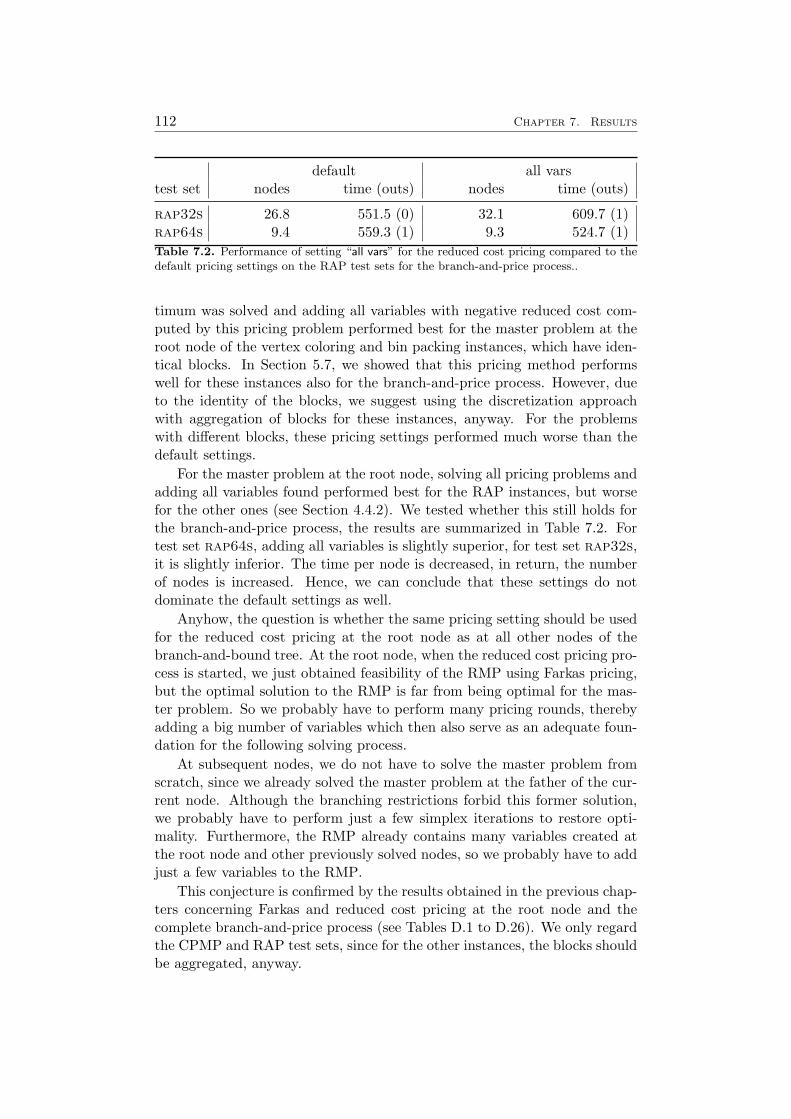
112 Chapter 7. Results
default all varstest set nodes time (outs) nodes time (outs)
rap32s 26.8 551.5 (0) 32.1 609.7 (1)rap64s 9.4 559.3 (1) 9.3 524.7 (1)Table 7.2. Performance of setting “all vars” for the reduced cost pricing compared to thedefault pricing settings on the RAP test sets for the branch-and-price process..
timum was solved and adding all variables with negative reduced cost com-puted by this pricing problem performed best for the master problem at theroot node of the vertex coloring and bin packing instances, which have iden-tical blocks. In Section 5.7, we showed that this pricing method performswell for these instances also for the branch-and-price process. However, dueto the identity of the blocks, we suggest using the discretization approachwith aggregation of blocks for these instances, anyway. For the problemswith different blocks, these pricing settings performed much worse than thedefault settings.
For the master problem at the root node, solving all pricing problems andadding all variables found performed best for the RAP instances, but worsefor the other ones (see Section 4.4.2). We tested whether this still holds forthe branch-and-price process, the results are summarized in Table 7.2. Fortest set rap64s, adding all variables is slightly superior, for test set rap32s,it is slightly inferior. The time per node is decreased, in return, the numberof nodes is increased. Hence, we can conclude that these settings do notdominate the default settings as well.
Anyhow, the question is whether the same pricing setting should be usedfor the reduced cost pricing at the root node as at all other nodes of thebranch-and-bound tree. At the root node, when the reduced cost pricing pro-cess is started, we just obtained feasibility of the RMP using Farkas pricing,but the optimal solution to the RMP is far from being optimal for the mas-ter problem. So we probably have to perform many pricing rounds, therebyadding a big number of variables which then also serve as an adequate foun-dation for the following solving process.
At subsequent nodes, we do not have to solve the master problem fromscratch, since we already solved the master problem at the father of the cur-rent node. Although the branching restrictions forbid this former solution,we probably have to perform just a few simplex iterations to restore opti-mality. Furthermore, the RMP already contains many variables created atthe root node and other previously solved nodes, so we probably have to addjust a few variables to the RMP.
This conjecture is confirmed by the results obtained in the previous chap-ters concerning Farkas and reduced cost pricing at the root node and thecomplete branch-and-price process (see Tables D.1 to D.26). We only regardthe CPMP and RAP test sets, since for the other instances, the blocks shouldbe aggregated, anyway.
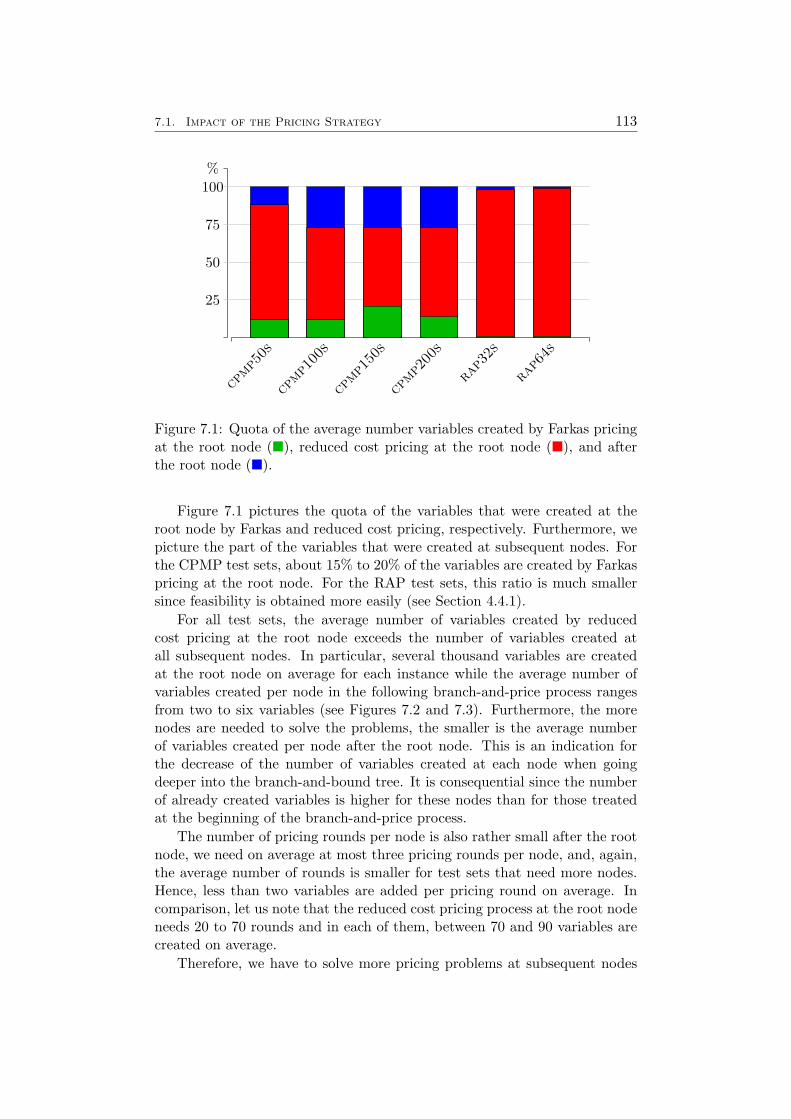
7.1. Impact of the Pricing Strategy 113
%
25
50
75
100
cpmp5
0s
cpmp1
00s
cpmp1
50s
cpmp2
00s
rap3
2s
rap6
4s
Figure 7.1: Quota of the average number variables created by Farkas pricingat the root node (�), reduced cost pricing at the root node (�), and afterthe root node (�).
Figure 7.1 pictures the quota of the variables that were created at theroot node by Farkas and reduced cost pricing, respectively. Furthermore, wepicture the part of the variables that were created at subsequent nodes. Forthe CPMP test sets, about 15% to 20% of the variables are created by Farkaspricing at the root node. For the RAP test sets, this ratio is much smallersince feasibility is obtained more easily (see Section 4.4.1).
For all test sets, the average number of variables created by reducedcost pricing at the root node exceeds the number of variables created atall subsequent nodes. In particular, several thousand variables are createdat the root node on average for each instance while the average number ofvariables created per node in the following branch-and-price process rangesfrom two to six variables (see Figures 7.2 and 7.3). Furthermore, the morenodes are needed to solve the problems, the smaller is the average numberof variables created per node after the root node. This is an indication forthe decrease of the number of variables created at each node when goingdeeper into the branch-and-bound tree. It is consequential since the numberof already created variables is higher for these nodes than for those treatedat the beginning of the branch-and-price process.
The number of pricing rounds per node is also rather small after the rootnode, we need on average at most three pricing rounds per node, and, again,the average number of rounds is smaller for test sets that need more nodes.Hence, less than two variables are added per pricing round on average. Incomparison, let us note that the reduced cost pricing process at the root nodeneeds 20 to 70 rounds and in each of them, between 70 and 90 variables arecreated on average.
Therefore, we have to solve more pricing problems at subsequent nodes
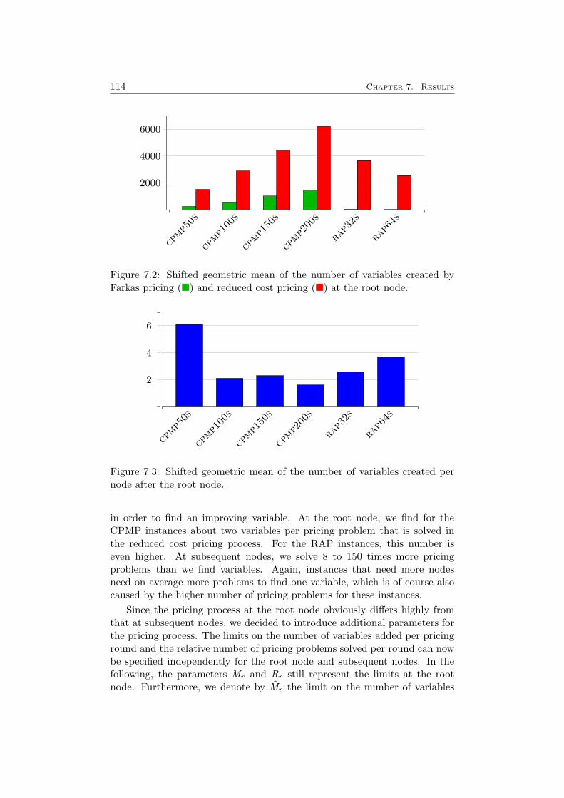
114 Chapter 7. Results
2000
4000
6000
cpmp5
0s
cpmp1
00s
cpmp1
50s
cpmp2
00s
rap3
2s
rap6
4s
Figure 7.2: Shifted geometric mean of the number of variables created byFarkas pricing (�) and reduced cost pricing (�) at the root node.
2
4
6
cpmp5
0s
cpmp1
00s
cpmp1
50s
cpmp2
00s
rap3
2s
rap6
4s
Figure 7.3: Shifted geometric mean of the number of variables created pernode after the root node.
in order to find an improving variable. At the root node, we find for theCPMP instances about two variables per pricing problem that is solved inthe reduced cost pricing process. For the RAP instances, this number iseven higher. At subsequent nodes, we solve 8 to 150 times more pricingproblems than we find variables. Again, instances that need more nodesneed on average more problems to find one variable, which is of course alsocaused by the higher number of pricing problems for these instances.
Since the pricing process at the root node obviously differs highly fromthat at subsequent nodes, we decided to introduce additional parameters forthe pricing process. The limits on the number of variables added per pricinground and the relative number of pricing problems solved per round can nowbe specified independently for the root node and subsequent nodes. In thefollowing, the parameters Mr and Rr still represent the limits at the rootnode. Furthermore, we denote by Mr the limit on the number of variables
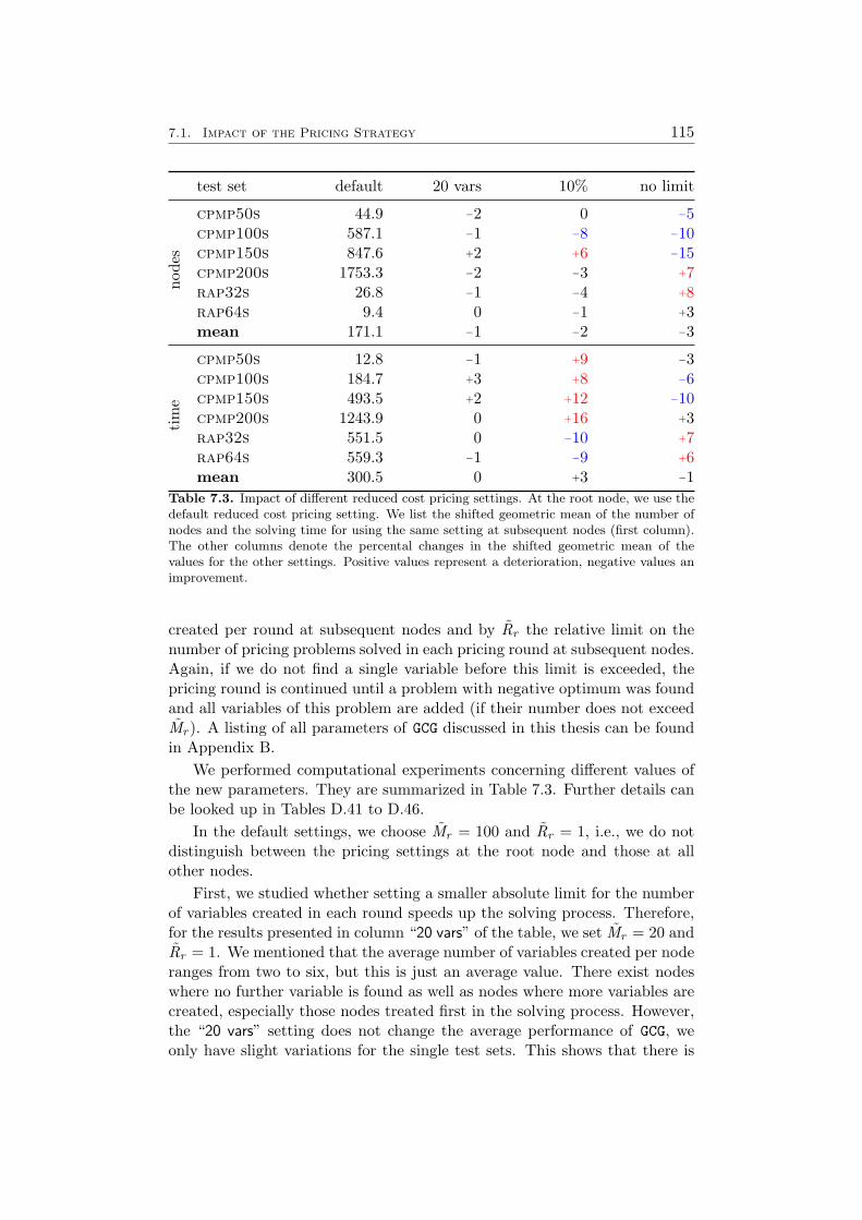
7.1. Impact of the Pricing Strategy 115
test set default 20 vars 10% no limitno
des
cpmp50s 44.9 −2 0 −5cpmp100s 587.1 −1 −8 −10cpmp150s 847.6 +2 +6 −15cpmp200s 1753.3 −2 −3 +7rap32s 26.8 −1 −4 +8rap64s 9.4 0 −1 +3mean 171.1 −1 −2 −3
tim
e
cpmp50s 12.8 −1 +9 −3cpmp100s 184.7 +3 +8 −6cpmp150s 493.5 +2 +12 −10cpmp200s 1243.9 0 +16 +3rap32s 551.5 0 −10 +7rap64s 559.3 −1 −9 +6mean 300.5 0 +3 −1
Table 7.3. Impact of different reduced cost pricing settings. At the root node, we use thedefault reduced cost pricing setting. We list the shifted geometric mean of the number ofnodes and the solving time for using the same setting at subsequent nodes (first column).The other columns denote the percental changes in the shifted geometric mean of thevalues for the other settings. Positive values represent a deterioration, negative values animprovement.
created per round at subsequent nodes and by Rr the relative limit on thenumber of pricing problems solved in each pricing round at subsequent nodes.Again, if we do not find a single variable before this limit is exceeded, thepricing round is continued until a problem with negative optimum was foundand all variables of this problem are added (if their number does not exceedMr ). A listing of all parameters of GCG discussed in this thesis can be foundin Appendix B.
We performed computational experiments concerning different values ofthe new parameters. They are summarized in Table 7.3. Further details canbe looked up in Tables D.41 to D.46.
In the default settings, we choose Mr = 100 and Rr = 1, i.e., we do notdistinguish between the pricing settings at the root node and those at allother nodes.
First, we studied whether setting a smaller absolute limit for the numberof variables created in each round speeds up the solving process. Therefore,for the results presented in column “20 vars” of the table, we set Mr = 20 andRr = 1. We mentioned that the average number of variables created per noderanges from two to six, but this is just an average value. There exist nodeswhere no further variable is found as well as nodes where more variables arecreated, especially those nodes treated first in the solving process. However,the “20 vars” setting does not change the average performance of GCG, weonly have slight variations for the single test sets. This shows that there is

116 Chapter 7. Results
only a small number of nodes where many variables are created so that thelimit of 20 variables created per pricing round is hardly ever exceeded.
Column “10%” presents the results for defining Rr = 0.1 and leavingMr = 100 unchanged. The number of nodes is slightly decreased for theCPMP instances as well as for the RAP instances. The time is increasedfor the CPMP instances while being decreased for the RAP instances. ForMr =∞ and Rr = 0.1 (column “no limit”), we obtain opposing results: Thenumber of nodes and the solving time for the CPMP instances is decreasedwhile these values are increased for the RAP instances.
This is a substantiation of our decision to introduce independent parame-ters for the root node on the one hand and all other nodes on the other hand.For the RAP instances, we have seen in Section 4.4, that adding all variablesat the root node performs better than the default settings, while adding justa small number performs much worse. However, for the subsequent nodes,the dominance is completely reverted: Adding a small number is remarkablybetter than adding all variables. The CPMP instances profit from a higherlimit in the branch-and-price process while a higher limit at the root nodeleads to a deterioration.
One reason for the aforementioned results might be the early terminationof the pricing process, which is enabled per default and was thus used for thesecomputations. By setting no limit on the number of variables we probablyintensify its impact, as described in the following.
Suppose we are at some node in the branch-and-bound tree and we haveto solve several pricing problems before finding a variable that can improvethe current solution. Without early termination, we have to perform anotherpricing round after adding this variable, regardless of whether we continuesolving the current pricing round and potentially add further variables, ornot. In particular, even if there do not exist further variables, we have tosolve all pricing problems to prove this in the next pricing round.
When enabling early termination, this changes: If we stop the pricinground, then we cannot compute a valid lower bound on the optimal objectivevalue of the master problem. In order to do this, we need the optimal solutionvalues of all pricing problems (see Section 4.2). Hence, we have to resolve theRMP and perform another pricing round. On the other hand, if we continuethe current pricing round and solve all pricing problems to optimality, we canprofit from that, even if we do not find further variables, since we get a validlower bound. With this bound, we can possibly stop the pricing process atthe current node due to early termination. It seems that this pays off for theCPMP instances since imposing no limit on the number of variables addedand therefore, solving all pricing problems in each round reduces the solvingtime in the shifted geometric mean.
However, the RAP instances have rather high optimal objective functionvalues so that even a small relative gap between dual bound and objectivefunction value of the RMP does not necessarily correspond to a small absolutegap that could allow the early termination of the pricing process. Hence, it
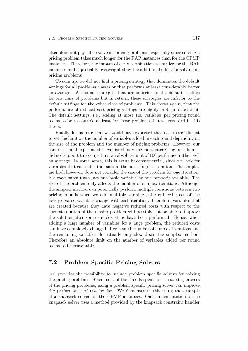
7.2. Problem Specific Pricing Solvers 117
often does not pay off to solve all pricing problems, especially since solving apricing problem takes much longer for the RAP instances than for the CPMPinstances. Therefore, the impact of early termination is smaller for the RAPinstances and is probably overweighted by the additional effort for solving allpricing problems.
To sum up, we did not find a pricing strategy that dominates the defaultsettings for all problems classes or that performs at least considerably betteron average. We found strategies that are superior to the default settingsfor one class of problems but in return, these strategies are inferior to thedefault settings for the other class of problems. This shows again, that theperformance of reduced cost pricing settings are highly problem dependent.The default settings, i.e., adding at most 100 variables per pricing roundseems to be reasonable at least for those problems that we regarded in thisthesis.
Finally, let us note that we would have expected that it is more efficientto set the limit on the number of variables added in each round depending onthe size of the problem and the number of pricing problems. However, ourcomputational experiments—we listed only the most interesting ones here—did not support this conjecture; an absolute limit of 100 performed rather wellon average. In some sense, this is actually consequential, since we look forvariables that can enter the basis in the next simplex iteration. The simplexmethod, however, does not consider the size of the problem for one iteration,it always substitutes just one basic variable by one nonbasic variable. Thesize of the problem only affects the number of simplex iterations. Althoughthe simplex method can potentially perform multiple iterations between twopricing rounds when we add multiple variables, the reduced costs of thenewly created variables change with each iteration. Therefore, variables thatare created because they have negative reduced costs with respect to thecurrent solution of the master problem will possibly not be able to improvethe solution after some simplex steps have been performed. Hence, whenadding a huge number of variables for a huge problem, the reduced costscan have completely changed after a small number of simplex iterations andthe remaining variables do actually only slow down the simplex method.Therefore an absolute limit on the number of variables added per roundseems to be reasonable.
7.2 Problem Specific Pricing Solvers
GCG provides the possibility to include problem specific solvers for solvingthe pricing problems. Since most of the time is spent for the solving processof the pricing problems, using a problem specific pricing solver can improvethe performance of GCG by far. We demonstrate this using the exampleof a knapsack solver for the CPMP instances. Our implementation of theknapsack solver uses a method provided by the knapsack constraint handler
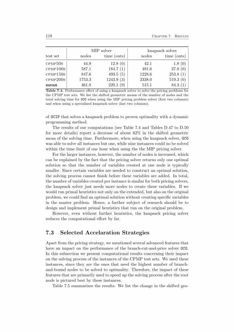
118 Chapter 7. Results
MIP solver knapsack solvertest set nodes time (outs) nodes time (outs)
cpmp50s 44.9 12.8 (0) 42.1 1.8 (0)cpmp100s 587.1 184.7 (1) 491.6 37.8 (0)cpmp150s 847.6 493.5 (5) 1228.6 253.8 (1)cpmp200s 1753.3 1243.9 (3) 2338.0 519.3 (0)mean 461.8 220.1 (9) 515.1 84.3 (1)Table 7.4. Performance effect of using a knapsack solver to solve the pricing problems forthe CPMP test sets. We list the shifted geometric means of the number of nodes and thetotal solving time for GCG when using the MIP pricing problem solver (first two columns)and when using a specialized knapsack solver (last two columns).
of SCIP that solves a knapsack problem to proven optimality with a dynamicprogramming method.
The results of our computations (see Table 7.4 and Tables D.47 to D.50for more details) report a decrease of about 62% in the shifted geometricmean of the solving time. Furthermore, when using the knapsack solver, GCGwas able to solve all instances but one, while nine instances could no be solvedwithin the time limit of one hour when using the the MIP pricing solver.
For the larger instances, however, the number of nodes is increased, whichcan be explained by the fact that the pricing solver returns only one optimalsolution so that the number of variables created at one node is typicallysmaller. Since certain variables are needed to construct an optimal solution,the solving process cannot finish before these variables are added. In total,the number of variables created per instance is similar for both pricing solvers,the knapsack solver just needs more nodes to create these variables. If wewould run primal heuristics not only on the extended, but also on the originalproblem, we could find an optimal solution without creating specific variablesin the master problem. Hence, a further subject of research should be todesign and implement primal heuristics that run on the original problem.
However, even without further heuristics, the knapsack pricing solverreduces the computational effort by far.
7.3 Selected Accelaration Strategies
Apart from the pricing strategy, we mentioned several advanced features thathave an impact on the performance of the branch-cut-and-price solver GCG.In this subsection we present computational results concerning their impacton the solving process of the instances of the CPMP test sets. We used theseinstances, since they are the ones that need the highest number of branch-and-bound nodes to be solved to optimality. Therefore, the impact of thesefeatures that are primarily used to speed up the solving process after the rootnode is pictured best by these instances.
Table 7.5 summarizes the results: We list the change in the shifted geo-
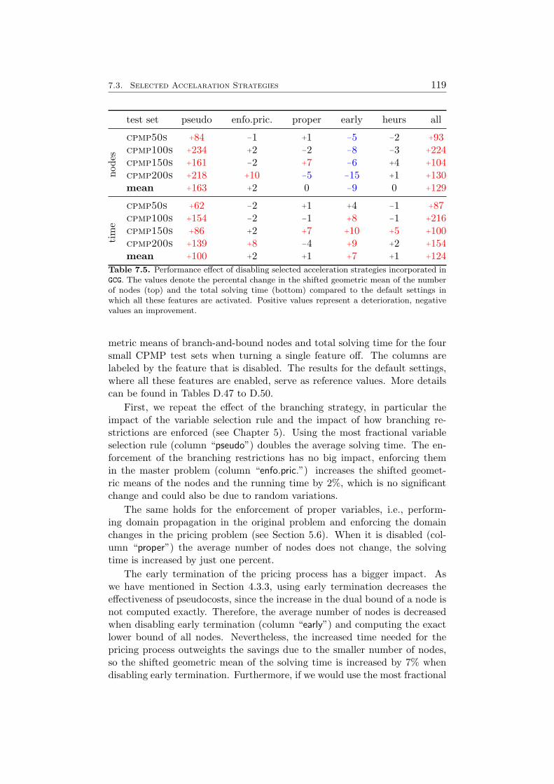
7.3. Selected Accelaration Strategies 119
test set pseudo enfo.pric. proper early heurs allno
des
cpmp50s +84 −1 +1 −5 −2 +93cpmp100s +234 +2 −2 −8 −3 +224cpmp150s +161 −2 +7 −6 +4 +104cpmp200s +218 +10 −5 −15 +1 +130mean +163 +2 0 −9 0 +129
tim
e
cpmp50s +62 −2 +1 +4 −1 +87cpmp100s +154 −2 −1 +8 −1 +216cpmp150s +86 +2 +7 +10 +5 +100cpmp200s +139 +8 −4 +9 +2 +154mean +100 +2 +1 +7 +1 +124
Table 7.5. Performance effect of disabling selected acceleration strategies incorporated inGCG. The values denote the percental change in the shifted geometric mean of the numberof nodes (top) and the total solving time (bottom) compared to the default settings inwhich all these features are activated. Positive values represent a deterioration, negativevalues an improvement.
metric means of branch-and-bound nodes and total solving time for the foursmall CPMP test sets when turning a single feature off. The columns arelabeled by the feature that is disabled. The results for the default settings,where all these features are enabled, serve as reference values. More detailscan be found in Tables D.47 to D.50.
First, we repeat the effect of the branching strategy, in particular theimpact of the variable selection rule and the impact of how branching re-strictions are enforced (see Chapter 5). Using the most fractional variableselection rule (column “pseudo”) doubles the average solving time. The en-forcement of the branching restrictions has no big impact, enforcing themin the master problem (column “enfo.pric.”) increases the shifted geomet-ric means of the nodes and the running time by 2%, which is no significantchange and could also be due to random variations.
The same holds for the enforcement of proper variables, i.e., perform-ing domain propagation in the original problem and enforcing the domainchanges in the pricing problem (see Section 5.6). When it is disabled (col-umn “proper”) the average number of nodes does not change, the solvingtime is increased by just one percent.
The early termination of the pricing process has a bigger impact. Aswe have mentioned in Section 4.3.3, using early termination decreases theeffectiveness of pseudocosts, since the increase in the dual bound of a node isnot computed exactly. Therefore, the average number of nodes is decreasedwhen disabling early termination (column “early”) and computing the exactlower bound of all nodes. Nevertheless, the increased time needed for thepricing process outweights the savings due to the smaller number of nodes,so the shifted geometric mean of the solving time is increased by 7% whendisabling early termination. Furthermore, if we would use the most fractional

120 Chapter 7. Results
variable selection rule rather than the pseudocost rule (although the formeris inferior to the latter), the performance effect of early termination wouldprobably be higher. Disabling early termination and obtaining more reliablepseudocosts would then not help the branching rule to decrease the numberof nodes, hence the time saved by early termination in the pricing processwould pay off even more.
Additionally, we tested the impact of using the convexification approachinstead of the discretization approach. Since the master problem essentiallystays the same, this actually just disables the use of primal heuristics in theextended SCIP instance. The results are listed in column “heurs”. We can seethat the primal heuristics in the extended problem do not have a big impacton the performance, most of the primal solutions are found as an integralsolution to the RMP, anyway. This shows that the default SCIP heuristicsare not very effective on the extended problem and we should think aboutimplementing further primal heuristics that take into account the branch-cut-and-price approach and use information of both the original es well asthe extended problem.
Finally, turning all these features off (column “all”) results in an increaseof more than 120% for the shifted geometric means of both the number ofnodes as well as the total running time. The smaller increase in the numberof nodes compared to disabling just the pseudocost variable selection rulefollows from the slowdown due to disabling the other features so that a smallernumber of nodes could be solved in case the timelimit was hit.
To summarize, the pseudocost variable selection rule has by far the biggestimpact on the performance of GCG for the regarded test sets of CPMP in-stances, followed by the early termination of the pricing process. The otherfeatures have a rather small impact on the performance of GCG.
7.4 Comparison to SCIP
In the last sections, we just tuned the performance of GCG. In this section,we finally answer the question whether the generic branch-cut-and-price ap-proach is competitive to an LP based branch-and-cut MIP solver. Since webased our implementation on the branch-cut-and-price framework SCIP, andSCIP with default plugins is a state-of-the-art branch-and-cut based MIPsolver, we compare this MIP solver to GCG on the complete test sets of thefour problem classes that we regard in this thesis. For both GCG and SCIP, weused the default settings. Like for all computations presented in this thesis,we used GCG version 0.7.0 and SCIP version 1.2.0.5. Further informationabout the test sets and the computational environment can be looked up inSection 3.3.
7.4. Comparison to SCIP 121
nodes timetest set items total mean total mean
bindata1-n1 50 520 1.7 196.5 1.2bindata1-n2 100 1681 3.4 922.7 4.4bindata1-n3 200 6222 11.3 4202.9 20.3Table 7.6. Computational results for GCG on the 180 instances of each size in the completebin packing test sets.
Identical Blocks: Bin Packing and Vertex Coloring
Bin packing and vertex coloring instances have identical blocks and a setpartitioning master problem, so the variables were aggregated and Ryan andFoster’s branching scheme was used. It is well-known that the Dantzig-Wolfedecomposition of the bin packing problem leads to strong dual bounds [60],so we were able to solve all 540 instances (180 instances with 50, 100, and 200items, respectively) in less than 90 minutes altogether. For each number ofitems, GCG solves the whole test set faster than SCIP solves the first instanceof the test set. The results for GCG are summarized in Table 7.6.
Also for our vertex coloring test set, GCG performs remarkably better thanSCIP which solved no more than twelve instances within the time limit of onehour per instance. GCG was able to solve 33 of the 39 instances. Furthermore,SCIP needs much more nodes than GCG and also the shifted geometric meanof the solving time per instance is about six times higher for SCIP than forGCG. These results are summarized in Table 7.7, more details can be foundin Table D.51.
SCIP GCGgap nodes time (outs) gap nodes time (outs)
19.5 3256.9 1073.3 (27) 8.7 64.3 176.1 (6)Table 7.7. Comparison of SCIP and GCG on the complete coloring test set (coloring-all).We list the shifted geometric means of the final gap, the number of branch-and-bound nodesand the solving time. Following the time, in brackets, we list the number of timeouts.
Different Blocks: The Capacited p-Median Problem
The capacitated p-median problem (CPMP) has multiple, different blocks,so they cannot be aggregated and branching on original variables is used. Inthe last sections, we already presented the impact of different settings on theperformance on GCG. Now, we want to compare it to SCIP, so we performedcomputational tests on the complete CPMP test sets, each of which consistsof 40 instances. We used default settings for both GCG and SCIP and imposeda time limit of one hour. Table 7.8 summarizes the results, more details canbe found in Tables D.52 to D.55.
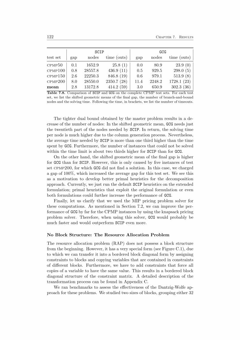
122 Chapter 7. Results
SCIP GCGtest set gap nodes time (outs) gap nodes time (outs)
cpmp50 0.1 1652.9 25.8 (1) 0.0 80.9 23.9 (0)cpmp100 0.8 28557.8 436.9 (11) 0.5 929.5 298.0 (5)cpmp150 2.6 22250.3 846.8 (19) 0.6 979.1 513.9 (8)cpmp200 8.0 28550.0 2350.7 (28) 11.4 2248.2 1728.1 (23)mean 2.8 13172.8 414.2 (59) 3.0 650.9 302.3 (36)Table 7.8. Comparison of SCIP and GCG on the complete CPMP test sets. For each testset, we list the shifted geometric means of the final gap, the number of branch-and-boundnodes and the solving time. Following the time, in brackets, we list the number of timeouts.
The tighter dual bound obtained by the master problem results in a de-crease of the number of nodes: In the shifted geometric mean, GCG needs justthe twentieth part of the nodes needed by SCIP. In return, the solving timeper node is much higher due to the column generation process. Nevertheless,the average time needed by SCIP is more than one third higher than the timespent by GCG. Furthermore, the number of instances that could not be solvedwithin the time limit is about two thirds higher for SCIP than for GCG.
On the other hand, the shifted geometric mean of the final gap is higherfor GCG than for SCIP. However, this is only caused by five instances of testset cpmp200, for which GCG did not find a solution. In this case, we chargeda gap of 100%, which increased the average gap for this test set. We see thisas a motivation to develop better primal heuristics for the decompositionapproach. Currently, we just run the default SCIP heuristics on the extendedformulation; primal heuristics that exploit the original formulation or evenboth formulations could further increase the performance of GCG.
Finally, let us clarify that we used the MIP pricing problem solver forthese computations. As mentioned in Section 7.2, we can improve the per-formance of GCG by far for the CPMP instances by using the knapsack pricingproblem solver. Therefore, when using this solver, GCG would probably bemuch faster and would outperform SCIP even more.
No Block Structure: The Resource Allocation Problem
The resource allocation problem (RAP) does not possess a block structurefrom the beginning. However, it has a very special form (see Figure C.1), dueto which we can transfer it into a bordered block diagonal form by assigningconstraints to blocks and copying variables that are contained in constraintsof different blocks. Furthermore, we have to add constraints that force allcopies of a variable to have the same value. This results in a bordered blockdiagonal structure of the constraint matrix. A detailed description of thetransformation process can be found in Appendix C.
We ran benchmarks to assess the effectiveness of the Dantzig-Wolfe ap-proach for these problems. We studied two sizes of blocks, grouping either 32
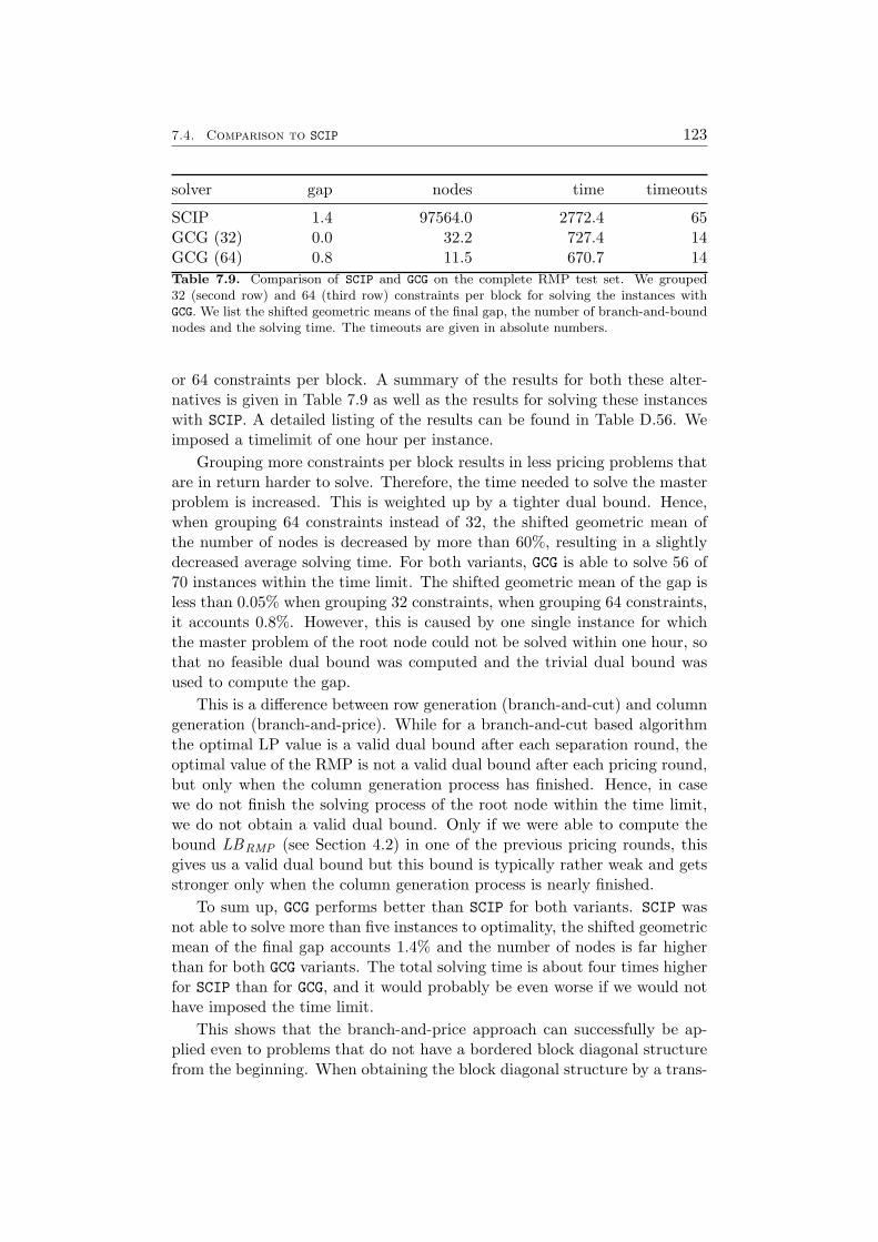
7.4. Comparison to SCIP 123
solver gap nodes time timeouts
SCIP 1.4 97564.0 2772.4 65GCG (32) 0.0 32.2 727.4 14GCG (64) 0.8 11.5 670.7 14Table 7.9. Comparison of SCIP and GCG on the complete RMP test set. We grouped32 (second row) and 64 (third row) constraints per block for solving the instances withGCG. We list the shifted geometric means of the final gap, the number of branch-and-boundnodes and the solving time. The timeouts are given in absolute numbers.
or 64 constraints per block. A summary of the results for both these alter-natives is given in Table 7.9 as well as the results for solving these instanceswith SCIP. A detailed listing of the results can be found in Table D.56. Weimposed a timelimit of one hour per instance.
Grouping more constraints per block results in less pricing problems thatare in return harder to solve. Therefore, the time needed to solve the masterproblem is increased. This is weighted up by a tighter dual bound. Hence,when grouping 64 constraints instead of 32, the shifted geometric mean ofthe number of nodes is decreased by more than 60%, resulting in a slightlydecreased average solving time. For both variants, GCG is able to solve 56 of70 instances within the time limit. The shifted geometric mean of the gap isless than 0.05% when grouping 32 constraints, when grouping 64 constraints,it accounts 0.8%. However, this is caused by one single instance for whichthe master problem of the root node could not be solved within one hour, sothat no feasible dual bound was computed and the trivial dual bound wasused to compute the gap.
This is a difference between row generation (branch-and-cut) and columngeneration (branch-and-price). While for a branch-and-cut based algorithmthe optimal LP value is a valid dual bound after each separation round, theoptimal value of the RMP is not a valid dual bound after each pricing round,but only when the column generation process has finished. Hence, in casewe do not finish the solving process of the root node within the time limit,we do not obtain a valid dual bound. Only if we were able to compute thebound LBRMP (see Section 4.2) in one of the previous pricing rounds, thisgives us a valid dual bound but this bound is typically rather weak and getsstronger only when the column generation process is nearly finished.
To sum up, GCG performs better than SCIP for both variants. SCIP wasnot able to solve more than five instances to optimality, the shifted geometricmean of the final gap accounts 1.4% and the number of nodes is far higherthan for both GCG variants. The total solving time is about four times higherfor SCIP than for GCG, and it would probably be even worse if we would nothave imposed the time limit.
This shows that the branch-and-price approach can successfully be ap-plied even to problems that do not have a bordered block diagonal structurefrom the beginning. When obtaining the block diagonal structure by a trans-

124 Chapter 7. Results
formation, a further direction of research should be to investigate how manyconstraints should be assigned to one block. As aforementioned, assigningmore constraints to one block makes the pricing problems harder to solve,but leads to better dual bounds. These properties have to be weighted upagainst each other.
Chapter 8
Summary, Conclusions andOutlook
In this thesis, we presented the theoretical background, implementational de-tails and computational results concerning the generic branch-cut-and-pricesolver GCG which was developed by the author of this thesis.
The foundation for this is the Dantzig-Wolfe decomposition for MIPswhich we presented in Chapter 2. It allows us to reformulate a general MIP,the original problem, into a problem with a huge number of variables, theextended problem. A subset of the constraints is transferred to the extendedproblem, the remaining constraints are implicitly treated and become partof the definition of the variables of the extended problem. We described twoways to perform this reformulation, the convexification and the discretizationapproach. The former is the more general one while the latter can reducesymmetry, if contained in the original problem. For both approaches, thedual bound—obtained by solving the relaxation of the extended problem—equals the Lagrangian dual bound and is typically stronger than the boundobtained by the LP relaxation. This is one of the main motivations for usingthe Dantzig-Wolfe decomposition and the branch-cut-and-price approach.
The branch-cut-and-price solver GCG is able to handle both approaches.The user has to provide the original problem and to define its structure,i.e., which of the constraints are treated implicitly and which of them aretransferred to the extended problem. GCG then performs the reformula-tion and solves both problems—the original and the extended problem—simultaneously. The general structure of GCG and the solving process waspresented in Chapter 3, as well as a short overview of the non-commercialbranch-cut-and-price framework SCIP on which our implementation is based.SCIP with default plugins is a state-of-the-art non-commercial MIP solverand was therefore also used to compare the branch-cut-and-price solver GCGto an LP based branch-and-cut MIP solver.
Since the extended problem has a huge number of variables, we do notsolve its LP relaxation, the master problem, explicitly, but use the concept of
125
126 Chapter 8. Summary, Conclusions and Outlook
column generation in order to do so. That is, we regard a restricted masterproblem (RMP) which contains just a subset of the variables and add vari-ables to the problem during the solving process whenever needed. Variableswhich potentially improve the solution are computed by a pricing process.For this, we solve one or more pricing problems which are given as MIPs andcontain the constraints that were not transferred to the extended problem.The concept of column generation, its application to the presented approach,and implementational details were presented in Chapter 4. Furthermore, weperformed computational experiments to assess the effectiveness of variouspricing strategies.
In order to compute an optimal integer solution, we use a branch-and-bound process. In combination with column generation, we thus obtain abranch-and-price algorithm. In Chapter 5, we described several branchingrules that fit into the branch-and-price approach. We implemented two ofthem, a branching on variables of the original problem and Ryan and Foster’sbranching scheme. The former one is used by most LP based branch-and-cut MIP solvers and can easily be transferred to the branch-cut-and-priceapproach. Ryan and Foster’s scheme can only be used for problems with aspecial structure in the extended problem; it can reduce symmetry when usedin combination with the discretization approach. Furthermore, we testedwhether the concept of pseudocosts, that is used by most state-of-the-artbranch-and-cut MIP solvers to select the variable on which branching is per-formed, can successfully be transferred to the branch-cut-and-price approach.It turned out that this is the case and using pseudocosts halves the shifted ge-ometric mean of the solving time for the class of capacited p-median problems.The other class of problems for which we tested the impact of pseudocosts,the RAP instances, are solved after a very small number of nodes so that theuse of pseudocosts does not pay off.
In Chapter 6, we described how the branch-and-price method can beturned into a branch-cut-and-price method by performing cutting plane sepa-ration. Cutting planes can be derived from either the original or the extendedproblem. We named pros and cons of both variants and described our imple-mentation of the former one. For general MIPs, we were able to find cuttingplanes this way, but the problems regarded in this thesis have a structurewhich does not allow the employed cutting plane separators to find cuttingplanes in the original problem. We used this as an occasion to compare thedual bounds at the root node obtained by GCG and SCIP. Even though SCIPtightened the dual bound by adding cutting planes, GCG obtained on averagea remarkably tighter dual bound for all regarded problems classes.
Finally, in Chapter 7, we presented some computational results concern-ing the overall performance of GCG. We tested the performance of pricingstrategies for the branch-cut-and-price process instead of doing so just forthe column generation process at the root node as it was done in Chap-ter 4. Additionally, we pictured the impact of using a problem specific solverto solve the pricing problems rather than solving them with a general MIP

127
solver. GCG provides the possibility to include such a solver and we did so fora knapsack solver which reduced the shifted geometric mean of the solvingtime by more than 60% for the class of capacited p-median problems. Fur-thermore, we reviewed some acceleration strategies, e.g., pseudocosts, earlytermination and the enforcement of proper variables, and their impact on theperformance of GCG.
Additionally, we compared the performance of GCG for the four problemsclasses regarded in this thesis with the performance of SCIP. These problemswere previously known to fit well into the branch-cut-and-price approach.However, former implementations for the problems classes were problem spe-cific. They used knowledge about the problem such as specialized pricingsolvers that can improve the performance by far as aforementioned. There-fore, one of the main goals of this thesis was to investigate whether thebranch-cut-and-price approach in the implemented generic form is still com-petitive to a state-of-the-art branch-and-cut MIP solver for these problems.It turned out that the generic branch-cut-and-price solver GCG still outper-forms SCIP although it does not use any problem specific knowledge exceptfor the structure of the problem.
Our main contribution is the development of the generic branch-cut-and-price solver GCG.
It provides the possibility to easily check whether a branch-cut-and-priceapproach for a problem is promising. Instead implementing a branch-cut-and-price solver form scratch or at least adding some problem specific plugins intoa branch-cut-and-price framework, one only needs to define the structure forthe decomposition in an additional file. The problem is then automaticallyreformulated by GCG and solved; pricing, branching and cutting plane separa-tion is performed in a generic way. If the approach turns out to be promising,the performance of GCG can further be enhanced by replacing generic partsof the solver by problem specific ones.
We studied how some concepts that are successfully used in LP basedbranch-and-cut MIP solvers can be transferred to the branch-cut-and-priceapproach, using the example of the capacited p-median problem. By perform-ing domain propagation in the original problem and transferring its resultsinto the extended problem, we enforce proper variables [96]. This slightlyimproved the performance of GCG. It turned out that using pseudocosts toselect the variable to branch on has a big impact: it essentially halved thesolving time. Furthermore, we tried to separate cutting planes in the originalproblem, but did not find any for the problems classes regarded in this the-sis. It seems that the reason for this is the special structure of the problems.However, for more general problems, cutting planes were found and couldimprove the solving capabilities of GCG.
For the RAP instances, we demonstrated that the branch-cut-and-priceapproach can perform well even if the problem does not have a bordered blockdiagonal structure right from the beginning. Since this problem has anotherspecial structure, we see this as an encouragement that this approach should

128 Chapter 8. Summary, Conclusions and Outlook
be tested for further problems with other special structures.There are still many concepts that should be investigated and integrated
to further enhance the solving capabilities of GCG.For the column generation process, apart from incorporating further prob-
lem specific pricing solvers, stabilization of the dual variables [64, 57] is oneof the most promising concepts. During the column generation process, thedual variables may highly oscillate. Through stabilization techniques, e.g.,penalizing big differences to the value of the dual variable in the last solution,this is reduced which typically improves the column generation performance.
For the branching process, it remains to be investigated whether reliabilitybranching—one of the most effective branching rules in LP based branch-and-cut—can successfully be transferred to the branch-cut-and-price approach.Furthermore, some more of the branching rules described in Chapter 5 shouldbe incorporating in GCG in future releases.
Also the separation capabilities of GCG could be further enhanced by en-abling separation of cutting planes in the extended problem and adding fur-ther separators for the original problem that do not need any informationabout the LP basis.
Finally, one of the primary targets for the future will be the developmentof further primal heuristics. On the one hand, we need heuristics that workon the original formulation and do not need to solve its LP relaxation. Onthe other hand, further heuristics in the extended problem that considerthe branch-cut-and-price approach could be investigated. For example, afterfinishing the column generation process at a node, one could try to solve thecorresponding extended problem, that contains just the subset of variablesalso contained in the RMP, to optimality with a branch-and-cut approachwithout further pricing of variables.
The most challenging question, however, is to investigate whether therereally is a significant share of problems for which the generic branch-cut-and-price approach is more effective than an LP based branch-and-cut algorithm,even when one does not know about a possibly contained structure. Thisrequires detecting whether it may pay off to reformulate the given MIP andto decide on how the reformulation is done.
Appendix A
Zusammenfassung (GermanSummary)
Viele Optimierungsprobleme lassen sich als gemischt-ganzzahlige Programme(MIPs) fomulieren. Obwohl das Losen von MIPs NP-schwer ist [86], lassensich viele dieser Probleme von aktuellen MIP-Losern in angemessener Zeitlosen (siehe z.B. Koch [55]). Die meisten dieser Loser basieren auf einemBranch-and-Cut-Ansatz, der eine Kombination aus der exakten Branch-and-Bound-Methode und Schnittebenenverfahren ist.
In dieser Arbeit haben wir eine andere Methode zum Losen von MIPsbetrachtet, die Branch-Cut-and-Price-Methode. Genau wie der Branch-and-Cut-Ansatz kombiniert sie Branch-and-Bound und Schnittebenenverfahren,zusatzlich verwendet sie jedoch noch das Konzept der Spaltengenerierung.Ihr Erfolg basiert auf einer Dekomposition des Problems in ein koordinieren-des Problem und ein oder mehrere Subprobleme. Das koordinierende Prob-lem enthalt exponentiell viele Variablen, die jedoch nicht explizit behandeltwerden, sondern implizit betrachtet und nur dann per Spaltengenerierungzum Problem hinzugefugt werden, wenn sie dessen aktuelle Losung verbessernkonnen. Um solche Variablen zu finden, werden die Subprobleme gelost,was oft sehr effektiv mit einem Algorithmus erfolgen kann, der eine spezielleStruktur der Probleme ausnutzt.
Diese Arbeit behandelt den vom Autor entwickelten generischen Branch-Cut-and-Price-Loser GCG.
Nach grundlegenden Definitionen und einem kurzen Uberblick uber dieGeschichte des Branch-Cut-and-Price-Ansatzes in Kapitel 1 stellen wir inKapitel 2 die Dantzig-Wolfe-Dekomposition fur MIPs vor, auf der unsereImplementation beruht.
Im 3. Kapitel prasentieren wir zunachst das Branch-Cut-and-Price-Framework SCIP, auf dem unser Branch-Cut-and-Price-Loser GCG aufbaut.Danach beschreiben wir die Struktur und den allgemeinen Losungsablauf desLosers GCG. Er benotigt neben dem originalen Problem weitere Informationenbezuglich dessen Struktur, anhand derer eine automatische Dekomposition
129

130 Appendix A. Zusammenfassung (German Summary)
durchgefuhrt wird. Im Anschluß werden sowohl das originale als auch dasdurch die Dekomposition erhaltene erweiterte Problem simultan gelost.
Die folgenden drei Kapitel behandeln die wichtigsten Bestandteile desBranch-Cut-and-Price-Losers GCG. In Kapitel 4 widmen wir uns dem Losungs-prozess der LP-Relaxierung des erweiterten Problems mit Hilfe von Spalten-generierung. Der Branching-Prozess ist Thema des 5. Kapitels, wahrend wirin Kapitel 6 die Generierung von Schnittebenen behandeln. In jedem dieserKapitel prasentieren wir zunachst einen Uberblick der zugrunde liegendenTheorie, legen dann implementatorische Entscheidungen dar und schließenmit Ergebnissen unserer Testrechnungen sowie deren Auswertung.
Im 7. Kapitel prasentieren wir weitere Testergebnisse. Wir betrachtenverschiedene Strategien bezuglich des Spaltengenerierungsprozesses. Nach-dem wir einige Varianten bereits im 4. Kapitel aufgrund ihrer schlechten Ef-fektivitat ausschließen konnten, zeigt sich, dass keine der anderen getestetenVarianten eindeutig uberlegen ist. Die standardmaßig verwendete Strategieliefert im Allgemeinen gute Ergebnisse, es gibt jedoch auch Alternativen,die auf einzelnen Klassen von Problemen uberlegen, auf anderen dafur je-doch unterlegen sind. Dies zeigt, dass die Effektivitat dieser Strategiensehr stark vom Problem und seiner Struktur abhangt. Um die Strukturder Subprobleme auszunutzen, bietet GCG die Moglichkeit, problemspezifischeLosungsmethoden einzubinden. Wird diese Moglichkeit nicht genutzt, werdendie Subprobleme fur die Spaltengenerierung, aufgrund des von GCG verfolgtengenerischen Ansatzes, standardmaßig als allgemeines MIP mit Hilfe von SCIPgelost. Wir testen den Einfluss einer problemspezifischen Losungsmethodeauf die Rechenzeit fur eine der betrachteten Klassen von Problem und erzie-len dadurch eine Beschleunigung von ca. 160%.
Des Weiteren untersuchen wir den Effekt einiger weiterer Methoden, dieden Losungsprozess beschleunigen sollen. Es ergibt sich, dass die Verwen-dung von Pseudokosten im Zusammenhang mit dem Branching-Prozess eineahnliche Verbesserung der Leistung bewirkt, wie sie schon fur Branch-and-Cut-Loser gezeigt wurde: Die durchschnittliche Losungszeit fur die betrach-tete Klasse von Problemen wird halbiert. Das fruhzeitige Beenden des Spal-tengenerierungsprozesses unter bestimmten Umstanden fuhrt immerhin nochzu einer Reduzierung der durchschnittlichen Losungszeit von ca. 7%. Dieweiteren getesteten Methoden haben wenig bis gar keinen Einfluss auf diedurchschnittliche Rechenzeit.
Abschließend ziehen wir einen Vergleich zwischen dem Branch-and-Cut-Loser SCIP und dem Branch-Cut-and-Price-Loser GCG. Die Eignung der ver-wendeten Probleme fur den Branch-Cut-and-Price-Ansatz war schon vorheraufgrund problemspezifischer Implementationen bekannt. Wir zeigen, dassGCG fur diese Probleme – trotz des generischen Ansatzes – bessere Ergebnisseals ein aktueller Branch-and-Cut-basierter MIP Loser erzielt.
Wir sehen das als Motivation, diesen Ansatz in Zukunft weiter zu verfol-gen und den generischen Branch-Cut-and-Price Loser GCG weiter auszubauen.
Appendix B
Notation and List ofParameters
We review the most important symbols used in this thesis. We start withthe most important general mathematical notation. After that, we list thesymbols used in the context of the Dantzig-Wolfe decomposition and theirmeaning. Finally, we present the parameters that can be used to tune GCG,the corresponding symbol used in the thesis and their effect.
General Mathematical Notation
Symbol Definition
N the natural numbers N = {1, 2, 3, . . . }Z the integer numbers Z = {. . . ,−3,−2,−1, 0, 1, 2, 3, . . . }Z+ the non-negative integer numbers Z+ = {0, 1, 2, 3, . . . }Q the rational numbersQ+ the non-negative rational numbers: Q+ = {x ∈ Q | x ≥ 0}R the real numbersR+ the non-negative real numbers: R+ = {x ∈ R | x ≥ 0}[n] the set [n] := {1, . . . , n} for n ∈ N
131
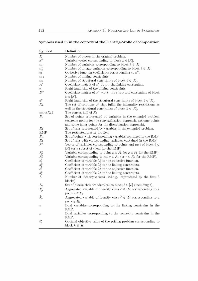
132 Appendix B. Notation and List of Parameters
Symbols used in in the context of the Dantzig-Wolfe decomposition
Symbol Definition
K Number of blocks in the original problem.xk Variable vector corresponding to block k ∈ [K].nk Number of variables corresponding to block k ∈ [K].n?
k Number of integer variables corresponding to block k ∈ [K].ck Objective function coefficients corresponding to xk.mA Number of linking constraints.mk Number of structural constraints of block k ∈ [K].Ak Coefficient matrix of xk w. r. t. the linking constraints.b Right-hand side of the linking constraints.Dk Coefficient matrix of xk w. r. t. the strcutural constraints of block
k ∈ [K].dk Right-hand side of the strcutural constraints of block k ∈ [K].Xk The set of solutions xk that fulfill the integrality restrictions as
well as the structural constraints of block k ∈ [K].conv(Xk) The convex hull of Xk.Pk Set of points represented by variables in the extended problem
(extreme points for the convexification approach, extreme pointsand some inner points for the discretization approach).
Rk Set of rays represented by variables in the extended problem.RMP The restricted master problem.Pk Set of points with corresponding variables contained in the RMP.Rk Set of rays with corresponding variables contained in the RMP.λk Vector of variables corresponding to points and rays of block k ∈
[K] (or a subset of them for the RMP).λk
p Variable corresponding to point p ∈ Pk (or p ∈ Pk for the RMP).λk
r Variable corresponding to ray r ∈ Rk (or r ∈ Rk for the RMP).ckp Coefficient of variable λk
p in the objective function.ak
p Coefficient of variable λkp in the linking constraints.
ckr Coefficient of variable λkr in the objective function.
akr Coefficient of variable λk
r in the linking constraints.L Number of identity classes (w.l.o.g. represented by the first L
blocks).K` Set of blocks that are identical to block ` ∈ [L] (including `).λ`
p Aggregated variable of identity class ` ∈ [L] corresponding to apoint p ∈ P`.
λ`r Aggregated variable of identity class ` ∈ [L] corresponding to a
ray r ∈ R`.π Dual variables corresponding to the linking constrains in the
RMP.ρ Dual variables corresponding to the convexity constrains in the
RMP.c?k Optimal objective value of the pricing problem corresponding to
block k ∈ [K].

133
Pricing Parameters
Parameter Symbol Description
maxvarsroundfarkas Mf Maximum number of variables created inone Farkas pricing round.
mipsrelfarkas Rf Relative number of pricing problems solvedin one Farkas pricing round. If this doesnot suffice to find new variables, pricing iscontinued until a problem was solved thatgives rise to new variables.
maxvarsroundredcostroot Mr Maximum number of variables created inone reduced cost pricing round (at first forall nodes, since Chapter 7 only for the rootnode).
mipsrelredcostroot Rr Relative number of pricing problems solvedin one reduced cost pricing round (at firstfor all nodes, since Chapter 7 only for theroot node). If this does not suffice to findnew variables, pricing is continued until aproblem was solved that gives rise to newvariables.
maxvarsroundredcost Mr Maximum number of variables created inone reduced cost pricing round at nodesafter the root node.
mipsrelredcost Rr Relative number of pricing problems solvedin one reduced cost pricing round at nodesafter the root node. If this does not sufficeto find new variables, pricing is continueduntil a problem was solved that gives riseto new variables.
maxsolsprob Mp Maximum number of variables created perpricing problem in a pricing round.
maxroundsredcost maxrounds Maximum number of reduced cost pricingrounds at a node.
sorting sorting Defines the sequence in which pricing prob-lems are solved.
onlybest onlybest Determines whether the best found vari-ables (TRUE ) are added instead of the firstfound ones (FALSE ).
useheur useheur Determines whether heuristic pricingshould be used (TRUE ).
In GCG, all these parameters are named “pricing/masterpricer/”, followedby the parameter name listed in the table.

134 Appendix B. Notation and List of Parameters
Branching Parameters
Parameter Symbol Description
usepseudocost usepseudocosts Determines whether the pseudocost(TRUE ) or the most fractional (FALSE )variable selection rule should be used forbranching on original variables.
enforcebycons Determines whether the branching restric-tions are enforced in the master prob-lem (TRUE ) or in the pricing problems(FALSE ).
In GCG, all these parameters are named “branching/orig/”, followed bythe parameter name listed in the table.
Relaxation Parameters
Parameter Symbol Description
discretization usedisc Determines whether the discretization ap-proach is used, if possible.
aggregateblocks aggrblocks Determines whether identical blocks areaggregated (TRUE ) or treated indepen-dently (FALSE ) (only when discretizationapproach used).
enforceproper enfoproper Determines whether proper variables areenforced (TRUE ) or not (FALSE ).
In GCG, all these parameters are named “relaxing/gcg/”, followed by theparameter name listed in the table.
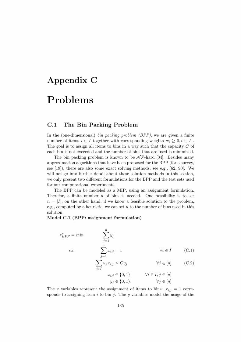
Appendix C
Problems
C.1 The Bin Packing Problem
In the (one-dimensional) bin packing problem (BPP), we are given a finitenumber of items i ∈ I together with corresponding weights wi ≥ 0, i ∈ I .The goal is to assign all items to bins in a way such that the capacity C ofeach bin is not exceeded and the number of bins that are used is minimized.
The bin packing problem is known to be NP-hard [34]. Besides manyapproximation algorithms that have been proposed for the BPP (for a survey,see [19]), there are also some exact solving methods, see e.g., [62, 90]. Wewill not go into further detail about these solution methods in this section,we only present two different formulations for the BPP and the test sets usedfor our computational experiments.
The BPP can be modeled as a MIP, using an assignment formulation.Therefor, a finite number n of bins is needed. One possibility is to setn = |I|, on the other hand, if we know a feasible solution to the problem,e.g., computed by a heuristic, we can set n to the number of bins used in thissolution.Model C.1 (BPP: assignment formulation)
z?BPP = min
n∑j=1
yj
s.t.n∑
j=1
xi,j = 1 ∀i ∈ I (C.1)
∑i∈I
wixi,j ≤ Cyj ∀j ∈ [n] (C.2)
xi,j ∈ {0, 1} ∀i ∈ I, j ∈ [n]yj ∈ {0, 1}. ∀j ∈ [n]
The x variables represent the assignment of items to bins: xi,j = 1 corre-sponds to assigning item i to bin j. The y variables model the usage of the
135

136 Appendix C. Problems
bins: bin j is used if and only if yj = 1. Hence, in the assignment formula-tion, we minimize the number of bins that are used, while constraints (C.1)assure that each item is assigned to exactly one bin and constraints (C.2)guarantee that items are only assigned to bins that are used and that thebin’s capacity is not exceeded.
We distinguish the bins in this formulation although there actually is nodifference between two bins, so it is highly symmetric: For each solution, weobtain a huge number of equivalent solutions by permuting the bins. Thistypically leads to a poor performance when solving the BPP with a branch-and-cut method.
An alternative formulation is the so-called set partitioning formulation.It overcomes the symmetry and leads to a stronger dual bound [60], in return,it contains an exponential number of variables.
Model C.2 (BPP: set partitioning formulation)
z?BPP = min
∑S∈S
λS
s.t.∑S∈S:i∈S
λS = 1 ∀i ∈ I (C.3)
λS ∈ {0, 1} ∀S ∈ S
with S ={S ⊆ I |
∑i∈S wi ≤ C
}.
The set S contains all subsets of items that fit into one bin. In this for-mulation, we choose a minimal number of subsets S ⊆ S and assure byconstraints (C.3) that each item is part of exactly one of the chosen subsets.
By applying the Dantzig-Wolfe decomposition presented in Chapter 2to the assignment formulation of the bin packing problem, treating con-straints (C.1) as linking constraints and constraints (C.2) as structural con-straints, we can obtain to this formulation, too. Actually, we get the setpartitioning formulation mentioned above when we use the discretization ap-proach, aggregate identical blocks and omit the convexity constraints, thatare redundant in this case. If we used the convexification approach, we wouldget a slightly different model with n identical subsets Sj , one for each bin.
For our computational experiments, we used a part of the instances pro-vided at [84], in particular all instances with 50, 100, and 200 items containedin data set 1. We denote by bindata1-n1, bindata1-n2, and bindata1-n3the sets of instances with 50, 100, and 200 items, respectively. Each set canbe devided into nine classes with 20 instances each. The classes are definedby a capacity C ∈ {100, 120, 150} and the interval used to choose the weights.These weights are uniformly distributed random integer numbers chosen fromone of the intervals [1, 100], [20, 100], and [30, 100]. Because of the large num-ber of instances per test set, we also defined smaller test sets bindata1-n1s,

C.2. The Vertex Coloring Problem 137
bindata1-n2s, and bindata1-n3s with 18 instances per test set, two of eachclass. We will primary use these small test sets for the computations, onlyin Chapter 7, we present results for the complete test sets, too.
For the assignment formulation of an instance, we need a maximum num-ber n of used bins. We set n = 1.5·OPT with OPT being the optimal solutionvalue of the instance (listed at [84]). Furthermore, we used a set coveringapproach rather than a set partitioning approach, so the assignement con-straints (C.1) change to
n∑j=1
xi,j ≥ 1 ∀i ∈ I (C.4)
assuring that each item is assigned to at least one bin. For a given solutionto the set covering model, a solution to the Model C.1 can be constructed byassigning each item to exactly one of the bins it is assigned to in the givensolution. The set covering formulation allows to construct feasible solutionsmore easily and is numerically more stable.
We treat constraints (C.4) as linking constraints and constraints (C.2) asstructural constraints when solving the bin packing problems with GCG.
C.2 The Vertex Coloring Problem
The vertex coloring problem (VCP) resembles the bin packing problem. Givenan undirected graph G = (V,E), we want to color the nodes V such that ad-jacent nodes get different colors and we use as few colors as possible. Insteadof assigning items to bins, we assign nodes to colors. In contrast to the binpacking problem, the set of nodes that may be assigned to one color is notlimited by a capacity, but by the edges of the graph: the nodes that get thesame color have to form a stable set in the graph, i.e., no two nodes of theset are adjacent.
The VCP is known to be NP-hard (see [34]). For a broader survey ofthe VCP, its applications as well as algorithmic and computational results,we refer to [72, 58]. In the following, we will present two formulations forthe VCP and the set of test instances that we used for our computationalexperiments.
The first possible formulation of the VCP is the following assignmentformulation. It needs a limited number n of colors. For example, we canalways set n = |V |, which is an upper bound on the number of colors needed.If we know a feasible solution to the problem, e.g., computed by a heuristic,we can also set n to the number of colors needed for this solution.

138 Appendix C. Problems
Model C.3 (VCP: assignment formulation)
z?V CP = min
n∑j=1
yj
s.t.n∑
j=1
xv,j = 1 ∀v ∈ V (C.5)
xv,j ≤ yj ∀v ∈ V, j ∈ [n] (C.6)xu,j + xv,j ≤ 1 ∀e = (u, v) ∈ E, j ∈ [n] (C.7)
xv,j ∈ {0, 1} ∀v ∈ V, j ∈ [n]yj ∈ {0, 1} ∀j ∈ [n]
The x variables represent the assignment of nodes to colors: xv,j = 1 if andonly if node v gets color j. The y variables correspond to the usage of thecolors, color j is used if and only if yj = 1. Constraints (C.5) assure thateach node gets exactly one color and constraints (C.6) guarantee that they variables are set correctly. Finally, constraints (C.7) ensure that adjacentnodes get different colors.
The assignment formulation has two essential drawbacks: There actuallyis no difference between the colors, but we have to distinguish them in themodel, so it contains a high degree of symmetry. For each solution, bypermuting the colors, we get a huge set of equivalent solutions. On theother hand, the LP relaxation of Model C.3 is extremely weak: By settingy1 = y2 = 1 and xv,1 = xv,2 = 1
2 for each node v ∈ V , we can construct afeasible solution of the relaxation with value 2 for each graph.
In order to overcome these drawbacks, we can formulate the VCP as aset partitioning problem with an exponential number of variables.
Model C.4 (VCP: set partitioning formulation)
z?V CP = min
∑S∈S
λS
s.t.∑S∈S:v∈S
λS = 1 ∀v ∈ V (C.8)
λS ∈ {0, 1} ∀S ∈ S
with S = {S ⊆ V | u /∈ S ∨ v /∈ S ∀e = (u, v) ∈ E}
A minimum number of subsets S ⊆ S is chosen in a way such that each nodeis part of one of the subsets. In fact, this formulation looks quite similar tothe set partitioning formulation of the bin packing problem, except for thedefinition of the set S, that contains only stable sets this time.
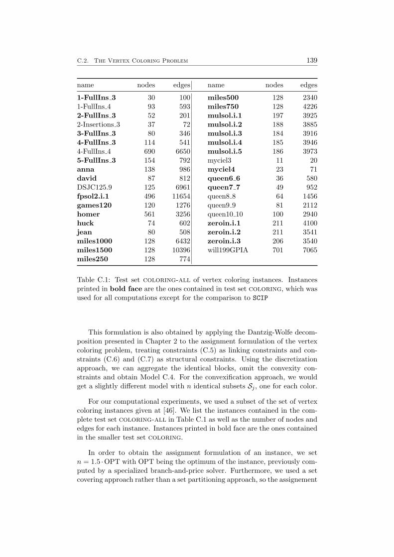
C.2. The Vertex Coloring Problem 139
name nodes edges name nodes edges
1-FullIns 3 30 100 miles500 128 23401-FullIns 4 93 593 miles750 128 42262-FullIns 3 52 201 mulsol.i.1 197 39252-Insertions 3 37 72 mulsol.i.2 188 38853-FullIns 3 80 346 mulsol.i.3 184 39164-FullIns 3 114 541 mulsol.i.4 185 39464-FullIns 4 690 6650 mulsol.i.5 186 39735-FullIns 3 154 792 myciel3 11 20anna 138 986 myciel4 23 71david 87 812 queen6 6 36 580DSJC125.9 125 6961 queen7 7 49 952fpsol2.i.1 496 11654 queen8 8 64 1456games120 120 1276 queen9 9 81 2112homer 561 3256 queen10 10 100 2940huck 74 602 zeroin.i.1 211 4100jean 80 508 zeroin.i.2 211 3541miles1000 128 6432 zeroin.i.3 206 3540miles1500 128 10396 will199GPIA 701 7065miles250 128 774
Table C.1: Test set coloring-all of vertex coloring instances. Instancesprinted in bold face are the ones contained in test set coloring, which wasused for all computations except for the comparison to SCIP
This formulation is also obtained by applying the Dantzig-Wolfe decom-position presented in Chapter 2 to the assignment formulation of the vertexcoloring problem, treating constraints (C.5) as linking constraints and con-straints (C.6) and (C.7) as structural constraints. Using the discretizationapproach, we can aggregate the identical blocks, omit the convexity con-straints and obtain Model C.4. For the convexification approach, we wouldget a slightly different model with n identical subsets Sj , one for each color.
For our computational experiments, we used a subset of the set of vertexcoloring instances given at [46]. We list the instances contained in the com-plete test set coloring-all in Table C.1 as well as the number of nodes andedges for each instance. Instances printed in bold face are the ones containedin the smaller test set coloring.
In order to obtain the assignment formulation of an instance, we setn = 1.5 ·OPT with OPT being the optimum of the instance, previously com-puted by a specialized branch-and-price solver. Furthermore, we used a setcovering approach rather than a set partitioning approach, so the assignement

140 Appendix C. Problems
constraints (C.5) change to
n∑j=1
xv,j ≥ 1 ∀v ∈ V (C.9)
assuring that each node gets at least one color. Given a solution to the setcovering model, a solution to the Model C.3 can be constructed by choosingexactly one of the assigned colors. The set covering formulation allows toconstruct feasible solutions more easily and is numerically more stable.
When solving the coloring instance with GCG, we treat constraints (C.9) aslinking constraints and constraints (C.6) and (C.7) as structural constraints.
C.3 The Capacitated p-Median Problem
The p-median problem (PMP) is a classical location problem. Let N be theset of nodes of a graph, representing sites where users are placed, and M ⊆ Nbe the set of potential location sites. The objective is to choose p medians(facilities) of this set M in a way such that the sum of the distances fromeach user to its nearest facility is minimized. The distance from user i ∈ Nto facility j ∈M is denoted by di,j ∈ Z+. The PMP is NP-hard [34].
The capacitated p-median problem (CPMP) is a generalization of thePMP, where each user i ∈ N has a demand qi ∈ Z+ while for each nodej ∈M , a facility placed at this node would have a production capacity of atmost Qj ∈ Z+. Again, we have to choose p medians and assign users to themedians in a way such that the sum of the distances from each user to theassigned facility is minimized. Additionally, we have to respect the capacityrestrictions, i.e., the total demand of nodes assigned to one facility must notexceed its capacity. For more details about the CPMP and solution methods,we refer to [15, 17] and the references given there.
The assignment formulation for the CPMP is the following:
Model C.5 (CPMP: assignment formulation)
z?CPMP = min
∑i∈N
∑j∈M
di,jxi,j
s.t.∑j∈M
xi,j = 1 ∀i ∈ N (C.10)
∑j∈M
yj = p (C.11)
∑i∈N
qixi,j ≤ Qjyj ∀j ∈M (C.12)
xi,j ∈ {0, 1} ∀i ∈ N, j ∈Myj ∈ {0, 1}. ∀j ∈M
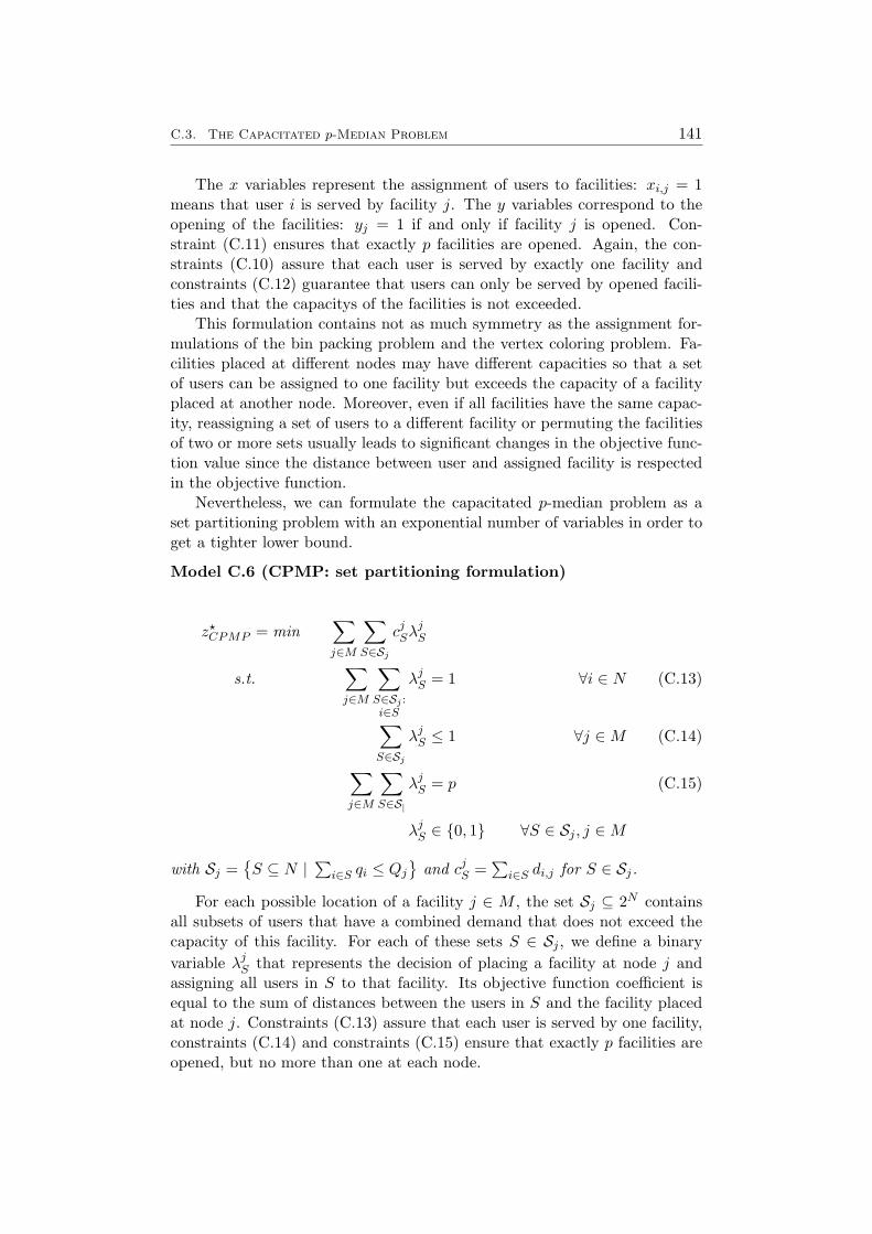
C.3. The Capacitated p-Median Problem 141
The x variables represent the assignment of users to facilities: xi,j = 1means that user i is served by facility j. The y variables correspond to theopening of the facilities: yj = 1 if and only if facility j is opened. Con-straint (C.11) ensures that exactly p facilities are opened. Again, the con-straints (C.10) assure that each user is served by exactly one facility andconstraints (C.12) guarantee that users can only be served by opened facili-ties and that the capacitys of the facilities is not exceeded.
This formulation contains not as much symmetry as the assignment for-mulations of the bin packing problem and the vertex coloring problem. Fa-cilities placed at different nodes may have different capacities so that a setof users can be assigned to one facility but exceeds the capacity of a facilityplaced at another node. Moreover, even if all facilities have the same capac-ity, reassigning a set of users to a different facility or permuting the facilitiesof two or more sets usually leads to significant changes in the objective func-tion value since the distance between user and assigned facility is respectedin the objective function.
Nevertheless, we can formulate the capacitated p-median problem as aset partitioning problem with an exponential number of variables in order toget a tighter lower bound.
Model C.6 (CPMP: set partitioning formulation)
z?CPMP = min
∑j∈M
∑S∈Sj
cjSλjS
s.t.∑j∈M
∑S∈Sj :i∈S
λjS = 1 ∀i ∈ N (C.13)
∑S∈Sj
λjS ≤ 1 ∀j ∈M (C.14)
∑j∈M
∑S∈S|
λjS = p (C.15)
λjS ∈ {0, 1} ∀S ∈ Sj , j ∈M
with Sj ={S ⊆ N |
∑i∈S qi ≤ Qj
}and cjS =
∑i∈S di,j for S ∈ Sj.
For each possible location of a facility j ∈ M , the set Sj ⊆ 2N containsall subsets of users that have a combined demand that does not exceed thecapacity of this facility. For each of these sets S ∈ Sj , we define a binaryvariable λj
S that represents the decision of placing a facility at node j andassigning all users in S to that facility. Its objective function coefficient isequal to the sum of distances between the users in S and the facility placedat node j. Constraints (C.13) assure that each user is served by one facility,constraints (C.14) and constraints (C.15) ensure that exactly p facilities areopened, but no more than one at each node.

142 Appendix C. Problems
Model C.6 can be obtained by applying the Dantzig-Wolfe decomposition(see Chapter 2) to the assignment formulation (Model C.5), treating con-straints (C.10) and (C.11) as linking constraints and constraints (C.12) asstructural constraints. This is also the structure that we use when solvingthe CPMP instances with GCG.
For our computational experiments, we used the set [14] of test instancesfor the CPMP, that were previously used in [15, 17]. The instances arenamed pFN − n, where N ∈ {50, 100, 150, 200} is the number of users,F ∈
{N10 ,⌈
N4
⌉,⌈
N3
⌉, 2N
5
}is the number of facilities that must be opened,
i.e., the value p of the problem definition, and n is a consecutive numberingof the ten instances for each combination of N and F . For each instance, allfacilities have the same capacity C =
⌈12N
p
⌉.
We defined four testsets cpmp50, cpmp100, cpmp150, and cpmp200containing the instances with 50, 100, 150, and 200 users, respectively. In or-der to reduce the computational effort, we also defined small testsetscpmp50s, cpmp100s, cpmp150s, and cpmp200s.
For each number of users N up to 150, we removed every second instancefrom the corresponding complete test set and obtained a small test set with20 instances, five instances for each number of facilities F . The instanceswith 200 users are the hardest ones, especially those with 50, 66, and 80facilities hit the time limit in most of the cases. Therefore, we chose onlythree instances for each number of facilities, and we chose primarily thoseinstances that could be solved within the time limit.
C.4 A Resource Allocation Problem
Finally, we regard a generalized knapsack problem [13] that does not have abordered block diagonal structure. Given a number of periods 1 ≤ n ≤ Nand items i ∈ I, each item has a profit pi, a weight wi, and a starting andending period. The periods are implicitly given by the sets I(n) ⊆ I, n ∈ [N ],that contain all items that are alive in period n. In each period, the knapsackhas capacity C and items consume capacity only during their life time. Thegoal is to maximize the sum of profits of the selected items in such a way thatfor each period, the capacity is not exceeded. The problem can be modelledin the following way:
Model C.7 (RAP)
z?RAP = max
∑i∈I
pixi
s.t.∑
i∈I(n)
wixi ≤ C ∀n ∈ [N ] (C.16)
xi ∈ {0, 1} ∀i ∈ I.
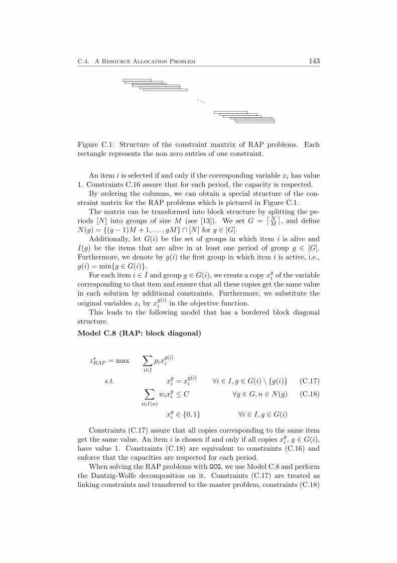
C.4. A Resource Allocation Problem 143
...
Figure C.1: Structure of the constraint maxtrix of RAP problems. Eachrectangle represents the non zero entries of one constraint.
An item i is selected if and only if the corresponding variable xi has value1. Constraints C.16 assure that for each period, the capacity is respected.
By ordering the columns, we can obtain a special structure of the con-straint matrix for the RAP problems which is pictured in Figure C.1.
The matrix can be transformed into block structure by splitting the pe-riods [N ] into groups of size M (see [13]). We set G =
⌈NM
⌉, and define
N(g) = {(g − 1)M + 1, . . . , gM} ∩ [N ] for g ∈ [G].Additionally, let G(i) be the set of groups in which item i is alive and
I(g) be the items that are alive in at least one period of group g ∈ [G].Furthermore, we denote by g(i) the first group in which item i is active, i.e.,g(i) = min{g ∈ G(i)}.
For each item i ∈ I and group g ∈ G(i), we create a copy xgi of the variable
corresponding to that item and ensure that all these copies get the same valuein each solution by additional constraints. Furthermore, we substitute theoriginal variables xi by xg(i)
i in the objective function.This leads to the following model that has a bordered block diagonal
structure.
Model C.8 (RAP: block diagonal)
z?RAP = max
∑i∈I
pixg(i)i
s.t. xgi = x
g(i)i ∀i ∈ I, g ∈ G(i) \ {g(i)} (C.17)∑
i∈I(n)
wixgi ≤ C ∀g ∈ G,n ∈ N(g) (C.18)
xgi ∈ {0, 1} ∀i ∈ I, g ∈ G(i)
Constraints (C.17) assure that all copies corresponding to the same itemget the same value. An item i is chosen if and only if all copies xg
i , g ∈ G(i),have value 1. Constraints (C.18) are equivalent to constraints (C.16) andenforce that the capacities are respected for each period.
When solving the RAP problems with GCG, we use Model C.8 and performthe Dantzig-Wolfe decomposition on it. Constraints (C.17) are treated aslinking constraints and transferred to the master problem, constraints (C.18)

144 Appendix C. Problems
go into the blocks. For the discretization approach, we obtain the followingextended problem:
Model C.9 (RAP: extended problem)
z?RAP = max
∑i∈I
pixi
s.t.∑
S∈Sg :i∈S
λgS =
∑S∈Sg(i):
i∈S
λg(i)S ∀i ∈ I, g ∈ G(i) \ {g(i)} (C.19)
∑S∈Sg
λgS = 1 ∀g ∈ [G] (C.20)
λgS ∈ {0, 1} ∀g ∈ [G], S ∈ Sg
with Sg ={S ⊆ I(g) |
∑i∈I(n)∩S wi ≤ C ∀n ∈ N(g)
}.
The set Sg contains all subsets of active items of group g that do notviolate the capacity constraints corresponding to the periods of this group.Constraints (C.20) ensure that for each group, exactly one of these sets ischosen, and constraints (C.19) enforce that items are either chosen in eachgroup in which they are active or in none of them.
For this type of problems, we used the test set described in [13], whichcontains seven classes, each of which contains ten instances. In the same wayas it is done there, we consider grouping 32 and 64 periods and defined thecorresponding test sets rap32 and rap64, respectively. In order to reducethe computational effort, we also defined small test sets rap32s and rap64s,that contain both the same 21 instances, three instances of each class. Asfar as possible, we chose instances that could be solved within a time limitof one hour. The complete test set is presented in Table C.2, the instancesprinted in bold face are the ones contained in the smaller test sets. Theywere used for most computations except for the comparison with SCIP wherewe used the complete test set. For each instance, we list the number of items(column “|I|”) and the number of periods (column “N”).

C.4. A Resource Allocation Problem 145
name |I| N name |I| N
new1 1 2071 768 new4 6 3774 1408new1 2 2422 896 new4 7 4164 1536new1 3 2756 1024 new4 8 4488 1664new1 4 3104 1152 new4 9 4786 1792new1 5 3433 1280 new4 10 5142 1920new1 6 3789 1408 new5 1 2916 768new1 7 4154 1536 new5 2 3424 896new1 8 4476 1664 new5 3 3832 1024new1 9 4797 1792 new5 4 4316 1152new1 10 5129 1920 new5 5 4771 1280new2 1 2071 768 new5 6 5403 1408new2 2 2422 896 new5 7 5793 1536new2 3 2756 1024 new5 8 6167 1664new2 4 3104 1152 new5 9 6800 1792new2 5 3433 1280 new5 10 7241 1920new2 6 3789 1408 new6 1 5210 768new2 7 4154 1536 new6 2 6057 896new2 8 4476 1664 new6 3 6901 1024new2 9 4797 1792 new6 4 7737 1152new2 10 5129 1920 new6 5 8656 1280new3 1 4948 768 new6 6 9370 1408new3 2 5769 896 new6 7 10271 1536new3 3 6721 1024 new6 8 11057 1664new3 4 7382 1152 new6 9 11992 1792new3 5 8266 1280 new6 10 13025 1920new3 6 9002 1408 new7 1 3117 768new3 7 9865 1536 new7 2 3594 896new3 8 10661 1664 new7 3 4176 1024new3 9 11448 1792 new7 4 4671 1152new3 10 12498 1920 new7 5 5209 1280new4 1 2071 768 new7 6 5628 1408new4 2 2422 896 new7 7 6215 1536new4 3 2763 1024 new7 8 6730 1664new4 4 3103 1152 new7 9 7172 1792new4 5 3434 1280 new7 10 7709 1920
Table C.2: Test set of RAP instances. Instances printed in bold face arethe ones contained in the small test sets rap32s and rap64s, which wereused for all computations except for the comparison to SCIP

146 Appendix C. Problems
Appendix D
Tables
In this chapter, we present the results of our test runs in detail. The tablesall organized as follows. Let us clarify that all time measurements are givenin seconds.
Tables D.1 to D.10 provide information about the Farkas pricing processat the root node, Tables D.11 to D.20 list details about the reduced cost pric-ing process at the root node. Each table pictures the results for one test set,the rows belong to different settings that are described in the correspondingsection. The columns list the number of pricing rounds, the number of pric-ing problems that were solved, the number of variables that were created, thepricing time, the LP solving time, the total time and the number of time outs.Except for the number of time outs, all values are shifted geometric meansof the values of the individual instances of the test set. In the tables corre-sponding to reduced cost pricing, the first five columns list just the valuescorresponding to reduced cost pricing, i.e., we substracted for each instancethe values belonging to Farkas pricing. The total time listed, however, is thetotal solving time of the master problem.
Tables D.21 to D.30 provide details about the branch-and-price processfor the single test sets. They are constructed in the same way as the previoustables, except for two additional columns that list the number of branch-and-bound nodes and the final gap.
Tables D.31 to D.40 present detailed results about the dual bound ob-tained at the root node. These results are summarized in Section 6.4. Welist for each instance the optimal objective function value, if it is not known,we list the objective function value of the best known solution and indicatethis with a star (*) behind the value. In the next columns, the dual bound,the gap to the optimal or best known solution and the solving time of theroot node are listed for GCG as well as for SCIP with two different settings.Setting “SCIP all cuts” corresponds to SCIP with default separation settings,setting “SCIP no base” to SCIP without using cuts that need informationabout the current LP basis. The dual bound and the gap obtained by SCIPis colored red for an instance if GCG computed the tighter dual bound. IfSCIP obtained the tighter dual bound, it is colored blue. For both SCIP
147

148 Appendix D. Tables
settings, we disabled strong branching and used most infeasible branching.Strong branching increased the solving time of the root node and can lead tostronger dual bounds which would distort the results since we just want tocompare the dual bounds after the relaxation is solved.
Tables D.41 to D.46 provide details about the computational experimentsconcerning reduced cost pricing that are summarized in Section 7.1 EachTable corresponds to one test set, the rows correspond to the single instancesof the test set. For each of the settings listed in the head row, we presentthe number of variables created during the solving process, the final gap, thenumber of branch-and-bound nodes and the total solving time in seconds. Asolving time of 3.600 denotes that the time limit of one hour was hit.
Tables D.47 to D.50 present details about the computational experimentssummarized in Sections 7.2 and 7.3. Each Table corresponds to one test set,the rows correspond to the single instances of the test set. For each of thesettings listed in the head row, we present the final gap, the number ofbranch-and-bound nodes and the total solving time in seconds. A solvingtime of 3.600 denotes that the time limit of one hour was hit.
Finally, Tables D.51 to D.56 present detailed comparisons of GCG andSCIP for the complete vertex coloring and CPMP test sets as well as for thecomplete RAP test set, with both variants described in Section C.4, assigningeither 32 or 64 constraints to one block. These results are summarized andinterpreted in Section 7.4.
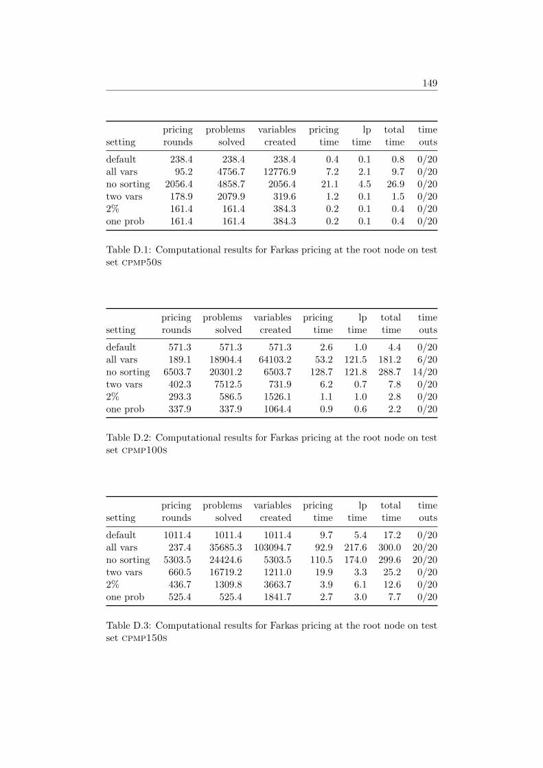
149
pricing problems variables pricing lp total timesetting rounds solved created time time time outs
default 238.4 238.4 238.4 0.4 0.1 0.8 0/20all vars 95.2 4756.7 12776.9 7.2 2.1 9.7 0/20no sorting 2056.4 4858.7 2056.4 21.1 4.5 26.9 0/20two vars 178.9 2079.9 319.6 1.2 0.1 1.5 0/202% 161.4 161.4 384.3 0.2 0.1 0.4 0/20one prob 161.4 161.4 384.3 0.2 0.1 0.4 0/20
Table D.1: Computational results for Farkas pricing at the root node on testset cpmp50s
pricing problems variables pricing lp total timesetting rounds solved created time time time outs
default 571.3 571.3 571.3 2.6 1.0 4.4 0/20all vars 189.1 18904.4 64103.2 53.2 121.5 181.2 6/20no sorting 6503.7 20301.2 6503.7 128.7 121.8 288.7 14/20two vars 402.3 7512.5 731.9 6.2 0.7 7.8 0/202% 293.3 586.5 1526.1 1.1 1.0 2.8 0/20one prob 337.9 337.9 1064.4 0.9 0.6 2.2 0/20
Table D.2: Computational results for Farkas pricing at the root node on testset cpmp100s
pricing problems variables pricing lp total timesetting rounds solved created time time time outs
default 1011.4 1011.4 1011.4 9.7 5.4 17.2 0/20all vars 237.4 35685.3 103094.7 92.9 217.6 300.0 20/20no sorting 5303.5 24424.6 5303.5 110.5 174.0 299.6 20/20two vars 660.5 16719.2 1211.0 19.9 3.3 25.2 0/202% 436.7 1309.8 3663.7 3.9 6.1 12.6 0/20one prob 525.4 525.4 1841.7 2.7 3.0 7.7 0/20
Table D.3: Computational results for Farkas pricing at the root node on testset cpmp150s

150 Appendix D. Tables
pricing problems variables pricing lp total timesetting rounds solved created time time time outs
default 1457.7 1457.7 1457.7 30.4 17.6 57.6 0/12all vars 266.7 53404.0 127254.4 134.8 158.7 299.9 12/12no sorting 3301.2 28155.6 3301.2 156.9 70.1 299.3 12/12two vars 898.4 28869.0 1649.2 51.5 8.7 68.2 1/122% 582.7 2330.5 6791.0 8.9 25.2 44.7 0/12one prob 700.8 700.8 2676.9 5.4 8.4 20.1 0/12
Table D.4: Computational results for Farkas pricing at the root node on testset cpmp200s
pricing problems variables pricing lp total timesetting rounds solved created time time time outs
default 241.1 241.1 241.1 3.8 0.1 6.8 0/28all vars 145.4 3256.9 4507.9 38.4 0.6 40.5 0/28no sorting 2240.2 3723.0 2240.2 168.9 14.7 243.8 11/28two vars 216.7 634.6 411.3 8.3 0.1 10.6 0/282% 222.9 263.1 424.6 4.2 0.1 7.0 0/28one prob 232.4 232.4 394.2 3.7 0.1 6.7 0/28disc all 172.3 172.3 256.0 2.8 0.1 6.2 0/28disc best 176.0 176.0 176.0 3.0 0.0 6.4 0/28
Table D.5: Computational results for Farkas pricing at the root node on testset coloring
pricing problems variables pricing lp total timesetting rounds solved created time time time outs
default 37.7 37.7 37.7 0.1 0.0 0.4 0/21all vars 37.7 1336.9 37.7 2.0 0.0 2.3 0/21no sorting 37.7 695.7 37.7 1.0 0.0 1.4 0/21two vars 37.7 1336.9 37.7 2.0 0.0 2.3 0/212% 37.7 46.3 37.7 0.1 0.0 0.4 0/21one prob 37.7 37.7 37.7 0.1 0.0 0.4 0/21
Table D.6: Computational results for Farkas pricing at the root node on testset rap32s

151
pricing problems variables pricing lp total timesetting rounds solved created time time time outs
default 19.0 19.0 19.0 0.0 -0.0 0.2 0/21all vars 19.0 345.5 19.0 0.8 -0.0 1.0 0/21no sorting 19.0 186.9 19.0 0.4 -0.0 0.6 0/21two vars 19.0 345.5 19.0 0.8 -0.0 1.0 0/212% 19.0 19.0 19.0 0.0 -0.0 0.2 0/21one prob 19.0 19.0 19.0 0.0 -0.0 0.2 0/21
Table D.7: Computational results for Farkas pricing at the root node on testset rap64s
pricing problems variables pricing lp total timesetting rounds solved created time time time outs
default 227.3 227.3 227.3 0.2 0.0 0.4 0/18all vars 60.4 2287.7 2725.0 1.6 0.1 1.9 0/18no sorting 1979.9 13984.2 1979.9 107.4 1.2 109.0 2/18two vars 172.1 952.8 324.9 0.6 0.0 0.8 0/182% 201.8 220.0 311.9 0.2 0.0 0.4 0/18one prob 219.1 219.1 312.2 0.2 0.0 0.4 0/18disc all 61.0 61.0 71.4 0.0 0.0 0.3 0/18disc best 63.2 63.2 63.2 0.0 0.0 0.3 0/18
Table D.8: Computational results for Farkas pricing at the root node on testset bindata1-n1s
pricing problems variables pricing lp total timesetting rounds solved created time time time outs
default 545.6 545.6 545.6 1.0 0.1 2.1 0/18all vars 120.0 8825.0 12047.5 9.8 0.5 11.4 0/18no sorting 4278.9 29857.4 4278.9 294.8 3.6 299.9 18/18two vars 415.3 3302.7 790.6 2.9 0.1 4.0 0/182% 344.8 695.2 968.6 0.8 0.1 1.9 0/18one prob 462.1 462.1 775.6 0.7 0.1 1.8 0/18disc all 122.0 122.0 166.0 0.1 0.0 1.1 0/18disc best 131.4 131.4 131.4 0.2 0.0 1.2 0/18
Table D.9: Computational results for Farkas pricing at the root node on testset bindata1-n2s
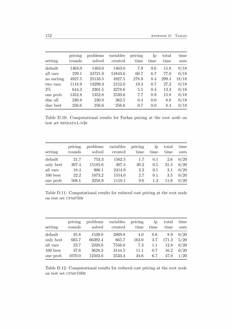
152 Appendix D. Tables
pricing problems variables pricing lp total timesetting rounds solved created time time time outs
default 1463.0 1463.0 1463.0 7.9 0.6 15.8 0/18all vars 229.1 34721.0 54843.6 60.7 6.7 77.0 0/18no sorting 4927.5 25133.5 4927.5 278.9 8.4 299.4 18/18two vars 1118.9 13299.3 2152.0 19.3 0.7 27.2 0/182% 644.2 2301.5 3278.6 5.5 0.4 13.3 0/18one prob 1352.8 1352.8 2539.6 7.7 0.9 15.8 0/18disc all 230.8 230.8 362.5 0.4 0.0 8.0 0/18disc best 256.6 256.6 256.6 0.7 0.0 8.4 0/18
Table D.10: Computational results for Farkas pricing at the root node ontest set bindata1-n3s
pricing problems variables pricing lp total timesetting rounds solved created time time time outs
default 21.7 753.3 1502.5 1.7 0.1 2.6 0/20only best 307.4 15185.6 307.4 30.2 0.5 31.4 0/20all vars 18.4 906.1 2414.9 2.2 0.1 3.1 0/20100 best 22.2 1073.2 1554.0 2.7 0.1 3.5 0/20one prob 508.1 3258.9 1110.1 9.6 1.3 11.6 0/20
Table D.11: Computational results for reduced cost pricing at the root nodeon test set cpmp50s
pricing problems variables pricing lp total timesetting rounds solved created time time time outs
default 35.8 1539.0 2869.8 4.0 0.6 8.9 0/20only best 665.7 66392.4 665.7 163.0 3.7 171.3 5/20all vars 23.7 2320.0 7556.0 7.3 1.1 12.8 0/20100 best 37.6 3628.3 3144.5 11.1 0.7 16.2 0/20one prob 1070.0 12503.0 2533.4 34.6 6.7 47.0 1/20
Table D.12: Computational results for reduced cost pricing at the root nodeon test set cpmp100s

153
pricing problems variables pricing lp total timesetting rounds solved created time time time outs
default 51.3 2515.1 4339.5 7.7 1.7 27.2 0/20only best 391.2 58091.2 391.2 276.0 5.2 299.6 20/20all vars 27.9 4078.4 14925.7 16.4 3.6 38.3 0/20100 best 53.8 7835.2 4766.0 29.5 2.2 49.9 0/20one prob 1579.9 19389.8 4009.0 64.3 17.1 107.7 5/20
Table D.13: Computational results for reduced cost pricing at the root nodeon test set cpmp150s
pricing problems variables pricing lp total timesetting rounds solved created time time time outs
default 69.6 3534.6 6073.8 12.6 4.2 73.4 0/12only best 151.5 29303.2 151.5 221.9 4.3 299.2 12/12all vars 31.1 6114.7 25224.5 29.6 8.2 95.2 1/12100 best 67.1 13175.2 6234.3 58.2 4.9 120.7 1/12one prob 1571.9 17727.2 4818.3 79.2 28.4 185.5 3/12
Table D.14: Computational results for reduced cost pricing at the root nodeon test set cpmp200s
pricing problems variables pricing lp total timesetting rounds solved created time time time outs
default 40.5 487.3 1695.5 33.6 0.5 40.9 0/28only best 45.4 834.7 45.4 51.3 0.2 58.3 0/28all vars 31.8 603.2 2487.1 41.3 0.5 47.8 0/28100 best 31.7 604.4 1397.9 40.7 0.3 47.1 0/28one prob 49.0 82.8 231.1 5.8 0.2 12.2 0/28disc all 70.2 71.3 292.0 6.2 0.2 11.4 0/28disc best 79.0 80.0 79.0 7.2 0.2 12.4 0/28
Table D.15: Computational results for reduced cost pricing at the root nodeon test set coloring
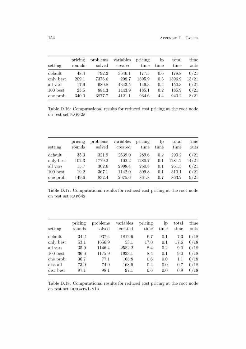
154 Appendix D. Tables
pricing problems variables pricing lp total timesetting rounds solved created time time time outs
default 48.4 792.2 3646.1 177.5 0.6 178.8 0/21only best 209.1 7376.6 208.7 1395.9 0.3 1396.9 13/21all vars 17.9 680.8 4343.5 149.3 0.4 150.3 0/21100 best 23.5 884.3 1443.9 185.1 0.2 185.9 0/21one prob 340.0 3877.7 4121.1 934.6 4.4 940.2 8/21
Table D.16: Computational results for reduced cost pricing at the root nodeon test set rap32s
pricing problems variables pricing lp total timesetting rounds solved created time time time outs
default 35.3 321.9 2539.0 289.6 0.2 290.2 0/21only best 102.3 1779.2 102.2 1280.7 0.1 1281.2 14/21all vars 15.7 302.6 2998.4 260.8 0.1 261.3 0/21100 best 19.2 367.1 1142.0 309.8 0.1 310.1 0/21one prob 149.6 832.4 2675.6 861.8 0.7 863.2 9/21
Table D.17: Computational results for reduced cost pricing at the root nodeon test set rap64s
pricing problems variables pricing lp total timesetting rounds solved created time time time outs
default 34.2 937.4 1812.6 6.7 0.1 7.3 0/18only best 53.1 1656.9 53.1 17.0 0.1 17.6 0/18all vars 35.9 1146.4 2582.2 8.4 0.2 9.0 0/18100 best 36.6 1175.9 1933.1 8.4 0.1 9.0 0/18one prob 36.7 77.1 165.8 0.6 0.0 1.1 0/18disc all 73.9 74.9 168.9 0.4 0.0 0.7 0/18disc best 97.1 98.1 97.1 0.6 0.0 0.9 0/18
Table D.18: Computational results for reduced cost pricing at the root nodeon test set bindata1-n1s

155
pricing problems variables pricing lp total timesetting rounds solved created time time time outs
default 79.1 3370.1 6618.5 50.3 0.8 54.3 0/18only best 129.8 8978.7 129.8 148.0 0.5 152.0 5/18all vars 77.2 5225.8 15971.5 82.3 1.9 88.0 2/18100 best 93.4 6354.1 7846.7 92.1 1.3 97.1 2/18one prob 74.3 152.3 480.5 5.8 0.3 8.6 0/18disc all 150.2 151.3 508.7 2.1 0.1 3.5 0/18disc best 222.8 223.8 222.8 3.9 0.2 5.4 0/18
Table D.19: Computational results for reduced cost pricing at the root nodeon test set bindata1-n2s
pricing problems variables pricing lp total timesetting rounds solved created time time time outs
default 132.6 6902.7 12848.5 101.8 4.2 126.6 2/18only best 108.0 15728.1 108.0 276.5 1.4 295.2 16/18all vars 98.6 13664.9 52565.7 236.1 13.5 274.2 14/18100 best 113.7 16725.2 11885.3 237.1 4.4 261.5 11/18one prob 114.0 276.5 839.3 9.1 1.9 31.3 0/18disc all 283.4 284.4 1159.4 5.9 0.8 15.6 0/18disc best 469.5 470.5 469.5 11.7 0.9 22.0 0/18
Table D.20: Computational results for reduced cost pricing at the root nodeon test set bindata1-n3s
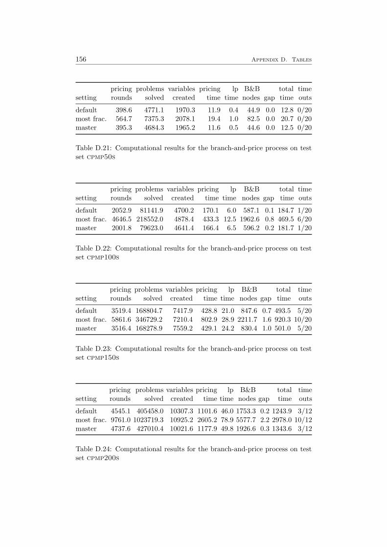
156 Appendix D. Tables
pricing problems variables pricing lp B&B total timesetting rounds solved created time time nodes gap time outs
default 398.6 4771.1 1970.3 11.9 0.4 44.9 0.0 12.8 0/20most frac. 564.7 7375.3 2078.1 19.4 1.0 82.5 0.0 20.7 0/20master 395.3 4684.3 1965.2 11.6 0.5 44.6 0.0 12.5 0/20
Table D.21: Computational results for the branch-and-price process on testset cpmp50s
pricing problems variables pricing lp B&B total timesetting rounds solved created time time nodes gap time outs
default 2052.9 81141.9 4700.2 170.1 6.0 587.1 0.1 184.7 1/20most frac. 4646.5 218552.0 4878.4 433.3 12.5 1962.6 0.8 469.5 6/20master 2001.8 79623.0 4641.4 166.4 6.5 596.2 0.2 181.7 1/20
Table D.22: Computational results for the branch-and-price process on testset cpmp100s
pricing problems variables pricing lp B&B total timesetting rounds solved created time time nodes gap time outs
default 3519.4 168804.7 7417.9 428.8 21.0 847.6 0.7 493.5 5/20most frac. 5861.6 346729.2 7210.4 802.9 28.9 2211.7 1.6 920.3 10/20master 3516.4 168278.9 7559.2 429.1 24.2 830.4 1.0 501.0 5/20
Table D.23: Computational results for the branch-and-price process on testset cpmp150s
pricing problems variables pricing lp B&B total timesetting rounds solved created time time nodes gap time outs
default 4545.1 405458.0 10307.3 1101.6 46.0 1753.3 0.2 1243.9 3/12most frac. 9761.0 1023719.3 10925.2 2605.2 78.9 5577.7 2.2 2978.0 10/12master 4737.6 427010.4 10021.6 1177.9 49.8 1926.6 0.3 1343.6 3/12
Table D.24: Computational results for the branch-and-price process on testset cpmp200s

157
pricing problems variables pricing lp B&B total timesetting rounds solved created time time nodes gap time outs
default 139.0 2361.6 3752.8 547.0 1.2 26.8 0.0 549.0 0/21most frac. 155.3 2643.1 3768.7 613.6 1.3 32.9 0.0 615.8 1/21master 142.1 2445.9 3764.6 567.8 1.3 27.3 0.0 569.8 0/21
Table D.25: Computational results for the branch-and-price process on testset rap32s
pricing problems variables pricing lp B&B total timesetting rounds solved created time time nodes gap time outs
default 74.6 617.8 2592.5 556.9 0.3 9.5 0.0 557.5 1/21most frac. 73.5 607.2 2586.6 547.1 0.2 9.4 0.0 547.7 1/21master 72.7 604.3 2590.9 547.6 0.2 8.8 0.0 548.1 1/21
Table D.26: Computational results for the branch-and-price process on testset rap64s
pricing problems variables pricing lp B&B total timesetting rounds solved created time time nodes gap time outs
conv. def. 299.1 1590.7 2931.5 13.9 0.3 8.6 0.0 14.4 0/18conv. 315.6 366.7 522.0 1.8 0.1 11.0 0.0 2.1 0/18disc. 143.4 142.0 243.5 0.9 0.0 2.2 0.0 1.1 0/18
Table D.27: Computational results for the branch-and-price process on testset bindata1-n1s
pricing problems variables pricing lp B&B total timesetting rounds solved created time time nodes gap time outs
conv. def. 744.1 4947.8 9649.5 98.2 2.4 24.7 0.0 102.3 0/18conv. 771.6 873.5 1415.0 13.2 1.0 20.8 0.0 15.1 0/18disc. 308.6 294.5 660.4 4.7 0.3 10.9 0.0 5.6 0/18
Table D.28: Computational results for the branch-and-price process on testset bindata1-n2s
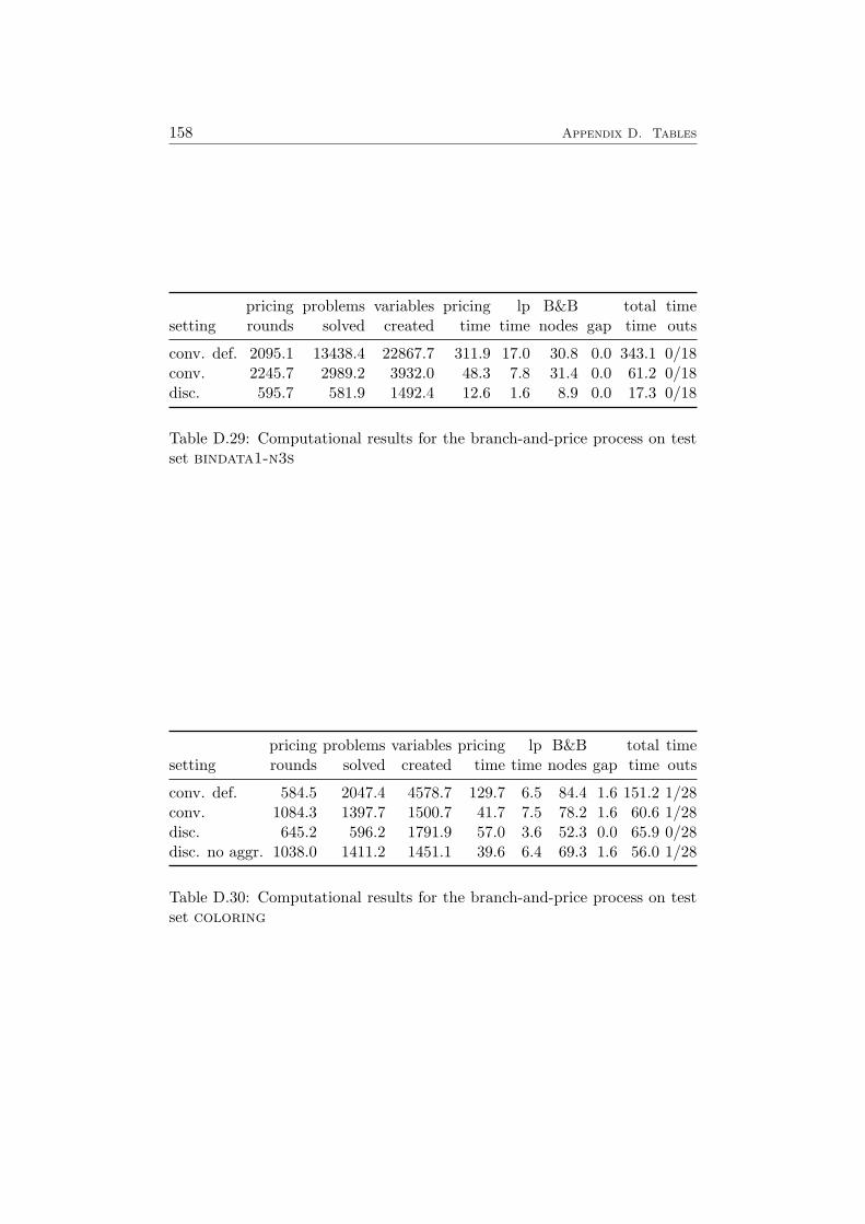
158 Appendix D. Tables
pricing problems variables pricing lp B&B total timesetting rounds solved created time time nodes gap time outs
conv. def. 2095.1 13438.4 22867.7 311.9 17.0 30.8 0.0 343.1 0/18conv. 2245.7 2989.2 3932.0 48.3 7.8 31.4 0.0 61.2 0/18disc. 595.7 581.9 1492.4 12.6 1.6 8.9 0.0 17.3 0/18
Table D.29: Computational results for the branch-and-price process on testset bindata1-n3s
pricing problems variables pricing lp B&B total timesetting rounds solved created time time nodes gap time outs
conv. def. 584.5 2047.4 4578.7 129.7 6.5 84.4 1.6 151.2 1/28conv. 1084.3 1397.7 1500.7 41.7 7.5 78.2 1.6 60.6 1/28disc. 645.2 596.2 1791.9 57.0 3.6 52.3 0.0 65.9 0/28disc. no aggr. 1038.0 1411.2 1451.1 39.6 6.4 69.3 1.6 56.0 1/28
Table D.30: Computational results for the branch-and-price process on testset coloring
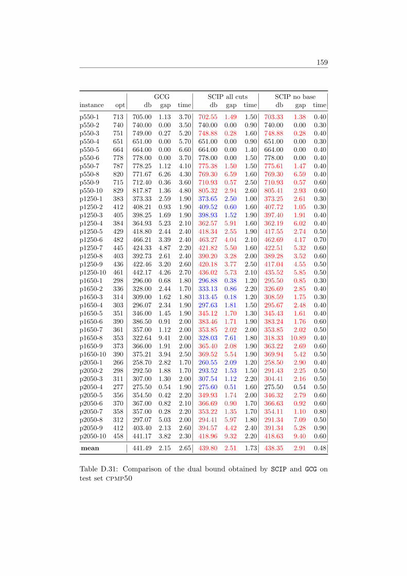
159
GCG SCIP all cuts SCIP no baseinstance opt db gap time db gap time db gap time
p550-1 713 705.00 1.13 3.70 702.55 1.49 1.50 703.33 1.38 0.40p550-2 740 740.00 0.00 3.50 740.00 0.00 0.90 740.00 0.00 0.30p550-3 751 749.00 0.27 5.20 748.88 0.28 1.60 748.88 0.28 0.40p550-4 651 651.00 0.00 5.70 651.00 0.00 0.90 651.00 0.00 0.30p550-5 664 664.00 0.00 6.60 664.00 0.00 1.40 664.00 0.00 0.40p550-6 778 778.00 0.00 3.70 778.00 0.00 1.50 778.00 0.00 0.40p550-7 787 778.25 1.12 4.10 775.38 1.50 1.50 775.61 1.47 0.40p550-8 820 771.67 6.26 4.30 769.30 6.59 1.60 769.30 6.59 0.40p550-9 715 712.40 0.36 3.60 710.93 0.57 2.50 710.93 0.57 0.60p550-10 829 817.87 1.36 4.80 805.32 2.94 2.60 805.41 2.93 0.60p1250-1 383 373.33 2.59 1.90 373.65 2.50 1.00 373.25 2.61 0.30p1250-2 412 408.21 0.93 1.90 409.52 0.60 1.60 407.72 1.05 0.30p1250-3 405 398.25 1.69 1.90 398.93 1.52 1.90 397.40 1.91 0.40p1250-4 384 364.93 5.23 2.10 362.57 5.91 1.60 362.19 6.02 0.40p1250-5 429 418.80 2.44 2.40 418.34 2.55 1.90 417.55 2.74 0.50p1250-6 482 466.21 3.39 2.40 463.27 4.04 2.10 462.69 4.17 0.70p1250-7 445 424.33 4.87 2.20 421.82 5.50 1.60 422.51 5.32 0.60p1250-8 403 392.73 2.61 2.40 390.20 3.28 2.00 389.28 3.52 0.60p1250-9 436 422.46 3.20 2.60 420.18 3.77 2.50 417.04 4.55 0.50p1250-10 461 442.17 4.26 2.70 436.02 5.73 2.10 435.52 5.85 0.50p1650-1 298 296.00 0.68 1.80 296.88 0.38 1.20 295.50 0.85 0.30p1650-2 336 328.00 2.44 1.70 333.13 0.86 2.20 326.69 2.85 0.40p1650-3 314 309.00 1.62 1.80 313.45 0.18 1.20 308.59 1.75 0.30p1650-4 303 296.07 2.34 1.90 297.63 1.81 1.50 295.67 2.48 0.40p1650-5 351 346.00 1.45 1.90 345.12 1.70 1.30 345.43 1.61 0.40p1650-6 390 386.50 0.91 2.00 383.46 1.71 1.90 383.24 1.76 0.60p1650-7 361 357.00 1.12 2.00 353.85 2.02 2.00 353.85 2.02 0.50p1650-8 353 322.64 9.41 2.00 328.03 7.61 1.80 318.33 10.89 0.40p1650-9 373 366.00 1.91 2.00 365.40 2.08 1.90 363.22 2.69 0.60p1650-10 390 375.21 3.94 2.50 369.52 5.54 1.90 369.94 5.42 0.50p2050-1 266 258.70 2.82 1.70 260.55 2.09 1.20 258.50 2.90 0.40p2050-2 298 292.50 1.88 1.70 293.52 1.53 1.50 291.43 2.25 0.50p2050-3 311 307.00 1.30 2.00 307.54 1.12 2.20 304.41 2.16 0.50p2050-4 277 275.50 0.54 1.90 275.60 0.51 1.60 275.50 0.54 0.50p2050-5 356 354.50 0.42 2.20 349.93 1.74 2.00 346.32 2.79 0.60p2050-6 370 367.00 0.82 2.10 366.69 0.90 1.70 366.63 0.92 0.60p2050-7 358 357.00 0.28 2.20 353.22 1.35 1.70 354.11 1.10 0.80p2050-8 312 297.07 5.03 2.00 294.41 5.97 1.80 291.34 7.09 0.50p2050-9 412 403.40 2.13 2.60 394.57 4.42 2.40 391.34 5.28 0.90p2050-10 458 441.17 3.82 2.30 418.96 9.32 2.20 418.63 9.40 0.60
mean 441.49 2.15 2.65 439.80 2.51 1.73 438.35 2.91 0.48
Table D.31: Comparison of the dual bound obtained by SCIP and GCG ontest set cpmp50
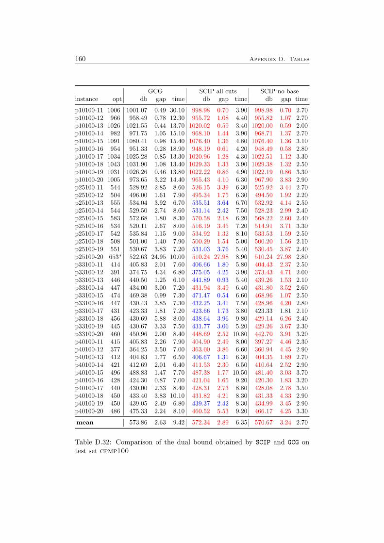
160 Appendix D. Tables
GCG SCIP all cuts SCIP no baseinstance opt db gap time db gap time db gap time
p10100-11 1006 1001.07 0.49 30.10 998.98 0.70 3.90 998.98 0.70 2.70p10100-12 966 958.49 0.78 12.30 955.72 1.08 4.40 955.82 1.07 2.70p10100-13 1026 1021.55 0.44 13.70 1020.02 0.59 3.40 1020.00 0.59 2.00p10100-14 982 971.75 1.05 15.10 968.10 1.44 3.90 968.71 1.37 2.70p10100-15 1091 1080.41 0.98 15.40 1076.40 1.36 4.80 1076.40 1.36 3.10p10100-16 954 951.33 0.28 18.90 948.19 0.61 4.20 948.49 0.58 2.80p10100-17 1034 1025.28 0.85 13.30 1020.96 1.28 4.30 1022.51 1.12 3.30p10100-18 1043 1031.90 1.08 13.40 1029.33 1.33 3.90 1029.38 1.32 2.50p10100-19 1031 1026.26 0.46 13.80 1022.22 0.86 4.90 1022.19 0.86 3.30p10100-20 1005 973.65 3.22 14.40 965.43 4.10 6.30 967.90 3.83 2.90p25100-11 544 528.92 2.85 8.60 526.15 3.39 6.30 525.92 3.44 2.70p25100-12 504 496.00 1.61 7.90 495.34 1.75 6.30 494.50 1.92 2.20p25100-13 555 534.04 3.92 6.70 535.51 3.64 6.70 532.92 4.14 2.50p25100-14 544 529.50 2.74 8.60 531.14 2.42 7.50 528.23 2.99 2.40p25100-15 583 572.68 1.80 8.30 570.58 2.18 6.20 568.22 2.60 2.40p25100-16 534 520.11 2.67 8.00 516.19 3.45 7.20 514.91 3.71 3.30p25100-17 542 535.84 1.15 9.00 534.92 1.32 8.10 533.53 1.59 2.50p25100-18 508 501.00 1.40 7.90 500.29 1.54 5.00 500.20 1.56 2.10p25100-19 551 530.67 3.83 7.20 531.03 3.76 5.40 530.45 3.87 2.40p25100-20 653* 522.63 24.95 10.00 510.24 27.98 8.90 510.24 27.98 2.80p33100-11 414 405.83 2.01 7.60 406.66 1.80 5.80 404.43 2.37 2.50p33100-12 391 374.75 4.34 6.80 375.05 4.25 3.90 373.43 4.71 2.00p33100-13 446 440.50 1.25 6.10 441.89 0.93 5.40 439.26 1.53 2.10p33100-14 447 434.00 3.00 7.20 431.94 3.49 6.40 431.80 3.52 2.60p33100-15 474 469.38 0.99 7.30 471.47 0.54 6.60 468.96 1.07 2.50p33100-16 447 430.43 3.85 7.30 432.25 3.41 7.50 428.96 4.20 2.80p33100-17 431 423.33 1.81 7.20 423.66 1.73 3.80 423.33 1.81 2.10p33100-18 456 430.69 5.88 8.00 438.64 3.96 9.80 429.14 6.26 2.40p33100-19 445 430.67 3.33 7.50 431.77 3.06 5.20 429.26 3.67 2.30p33100-20 460 450.96 2.00 8.40 448.69 2.52 10.80 442.70 3.91 3.20p40100-11 415 405.83 2.26 7.90 404.90 2.49 8.00 397.27 4.46 2.30p40100-12 377 364.25 3.50 7.00 363.00 3.86 6.60 360.94 4.45 2.90p40100-13 412 404.83 1.77 6.50 406.67 1.31 6.30 404.35 1.89 2.70p40100-14 421 412.69 2.01 6.40 411.53 2.30 6.50 410.64 2.52 2.90p40100-15 496 488.83 1.47 7.70 487.38 1.77 10.50 481.40 3.03 3.70p40100-16 428 424.30 0.87 7.00 421.04 1.65 9.20 420.30 1.83 3.20p40100-17 440 430.00 2.33 8.40 428.31 2.73 8.80 428.08 2.78 3.50p40100-18 450 433.40 3.83 10.10 431.82 4.21 8.30 431.33 4.33 2.90p40100-19 450 439.05 2.49 6.80 439.37 2.42 8.30 434.99 3.45 2.90p40100-20 486 475.33 2.24 8.10 460.52 5.53 9.20 466.17 4.25 3.30
mean 573.86 2.63 9.42 572.34 2.89 6.35 570.67 3.24 2.70
Table D.32: Comparison of the dual bound obtained by SCIP and GCG ontest set cpmp100
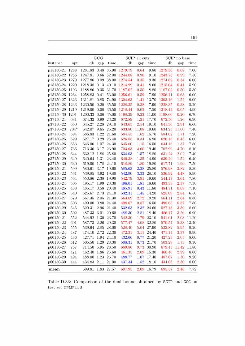
161
GCG SCIP all cuts SCIP no baseinstance opt db gap time db gap time db gap time
p15150-21 1288 1281.83 0.48 35.90 1279.79 0.64 9.80 1279.36 0.68 7.00p15150-22 1256 1247.81 0.66 52.00 1244.08 0.96 9.10 1243.73 0.99 7.50p15150-23 1279 1277.86 0.09 38.00 1274.54 0.35 9.30 1274.62 0.34 6.00p15150-24 1220 1218.38 0.13 40.10 1214.99 0.41 8.60 1215.04 0.41 5.90p15150-25 1193 1188.86 0.35 31.70 1187.02 0.50 8.80 1187.02 0.50 5.80p15150-26 1264 1258.83 0.41 53.00 1256.61 0.59 7.90 1256.11 0.63 6.00p15150-27 1323 1311.81 0.85 74.90 1304.63 1.41 13.70 1303.16 1.52 9.00p15150-28 1233 1230.50 0.20 35.50 1228.35 0.38 7.90 1228.35 0.38 5.20p15150-29 1219 1219.00 0.00 36.50 1218.44 0.05 7.50 1218.44 0.05 4.90p15150-30 1201 1200.33 0.06 35.00 1198.29 0.23 11.00 1198.60 0.20 6.70p37150-21 681 674.32 0.99 23.20 672.89 1.21 17.70 672.50 1.26 6.90p37150-22 660 645.27 2.28 29.10 643.65 2.54 19.10 641.36 2.91 6.60p37150-23 704* 642.07 9.65 26.20 633.80 11.08 19.60 634.23 11.00 7.40p37150-24 594 586.83 1.22 21.60 584.55 1.62 15.70 584.02 1.71 7.20p37150-25 629 627.17 0.29 25.40 626.85 0.34 16.90 626.16 0.45 6.00p37150-26 653 646.06 1.07 24.30 645.60 1.15 16.50 644.16 1.37 7.80p37150-27 736 713.36 3.17 23.90 703.63 4.60 19.40 702.99 4.70 8.10p37150-28 644 632.12 1.88 25.80 634.03 1.57 18.80 631.24 2.02 7.40p37150-29 649 640.64 1.31 23.40 640.38 1.35 14.90 639.29 1.52 6.40p37150-30 630 619.00 1.78 24.10 618.89 1.80 19.80 617.71 1.99 7.50p50150-21 599 580.61 3.17 19.60 585.63 2.28 25.80 576.98 3.82 8.30p50150-22 561 539.85 3.92 19.80 542.90 3.33 28.10 536.92 4.48 8.90p50150-23 564 550.86 2.38 19.90 542.79 3.91 19.60 544.17 3.64 7.80p50150-24 505 495.17 1.99 23.30 496.01 1.81 18.60 493.33 2.37 7.30p50150-25 488 485.17 0.58 20.40 485.91 0.43 11.80 484.71 0.68 7.10p50150-26 540 525.67 2.73 24.10 532.31 1.45 14.20 525.09 2.84 6.50p50150-27 579 567.35 2.05 21.30 563.69 2.72 19.20 564.11 2.64 8.80p50150-28 503 499.00 0.80 24.40 498.67 0.87 16.50 498.65 0.87 7.80p50150-29 545 529.31 2.96 21.40 532.63 2.32 24.60 527.13 3.39 8.60p50150-30 502 487.33 3.01 20.60 488.30 2.81 18.40 486.17 3.26 6.90p60150-21 552 544.92 1.30 23.70 542.30 1.79 23.10 541.01 2.03 11.20p60150-22 601 587.73 2.26 29.30 577.47 4.08 32.80 570.57 5.33 13.40p60150-23 555 539.64 2.85 28.00 528.40 5.04 27.90 523.82 5.95 9.20p60150-24 487 474.10 2.72 22.30 472.31 3.11 24.40 471.14 3.37 9.90p60150-25 436 427.71 1.94 24.10 432.66 0.77 21.20 427.23 2.05 8.00p60150-26 512 505.50 1.29 23.30 508.31 0.73 21.70 503.29 1.73 9.30p60150-27 757 714.50 5.95 28.50 689.86 9.73 30.90 679.43 11.42 11.80p60150-28 471 462.40 1.86 25.60 461.35 2.09 15.30 460.46 2.29 8.60p60150-29 494 488.00 1.23 26.70 488.77 1.07 17.40 487.67 1.30 9.20p60150-30 444 434.83 2.11 21.00 437.34 1.52 18.10 434.03 2.30 8.00
mean 699.81 1.83 27.57 697.95 2.09 16.79 695.57 2.48 7.72
Table D.33: Comparison of the dual bound obtained by SCIP and GCG ontest set cpmp150

162 Appendix D. Tables
GCG SCIP all cuts SCIP no baseinstance opt db gap time db gap time db gap time
p20200-31 1378 1372.09 0.43 89.30 1369.89 0.59 21.10 1369.94 0.59 11.30p20200-32 1424 1409.92 1.00 260.20 1403.15 1.49 22.50 1403.88 1.43 15.50p20200-33 1367 1361.85 0.38 73.60 1357.70 0.68 23.10 1358.93 0.59 12.30p20200-34 1385 1374.55 0.76 114.00 1372.29 0.93 28.80 1371.99 0.95 10.90p20200-35 1437 1430.73 0.44 72.90 1427.44 0.67 25.10 1427.81 0.64 12.70p20200-36 1382 1378.33 0.27 183.90 1376.21 0.42 25.20 1376.38 0.41 11.20p20200-37 1458 1454.25 0.26 83.80 1453.09 0.34 23.60 1452.69 0.37 12.90p20200-38 1382 1372.31 0.71 106.10 1368.66 0.97 21.70 1368.66 0.97 11.90p20200-39 1374 1369.69 0.31 72.90 1367.85 0.45 24.30 1367.70 0.46 10.90p20200-40 1416 1413.19 0.20 84.30 1411.54 0.32 28.10 1412.29 0.26 13.10p50200-31 728* 711.75 2.28 62.50 711.44 2.33 46.70 707.85 2.85 15.10p50200-32 878* 799.28 9.85 52.20 777.23 12.96 51.50 772.09 13.72 12.10p50200-33 760* 693.65 9.57 52.40 695.31 9.30 46.20 688.19 10.43 10.60p50200-34 858* 778.73 10.18 64.00 758.73 13.08 43.80 759.95 12.90 17.30p50200-35 752* 727.11 3.42 66.00 724.07 3.86 50.00 718.48 4.67 12.10p50200-36 701 692.22 1.27 64.50 693.09 1.14 53.30 687.40 1.98 15.20p50200-37 753 743.40 1.29 46.30 744.28 1.17 28.30 740.92 1.63 12.10p50200-38 749* 729.96 2.61 67.10 724.57 3.37 42.60 723.89 3.47 14.30p50200-39 722 712.62 1.32 67.90 715.60 0.89 33.20 711.60 1.46 12.80p50200-40 779* 737.54 5.62 52.70 731.76 6.46 59.80 726.92 7.16 12.40p66200-31 575 571.08 0.69 59.50 571.12 0.68 35.50 569.49 0.97 17.00p66200-32 860* 699.15 23.01 41.80 682.61 25.99 77.60 673.05 27.78 18.70p66200-33 648* 599.12 8.16 50.10 599.07 8.17 74.40 593.67 9.15 18.60p66200-34 729* 683.50 6.66 54.90 672.28 8.44 46.10 664.06 9.78 16.30p66200-35 615* 592.43 3.81 38.60 593.21 3.67 33.20 590.51 4.15 17.50p66200-36 580 569.51 1.84 47.60 569.21 1.90 52.30 565.48 2.57 15.30p66200-37 636* 616.50 3.16 46.60 616.49 3.16 34.10 614.93 3.43 15.20p66200-38 608 595.35 2.12 44.00 592.81 2.56 50.20 591.62 2.77 21.50p66200-39 589* 573.57 2.69 60.10 576.89 2.10 37.50 572.68 2.85 15.70p66200-40 632* 607.90 3.96 50.20 613.99 2.93 62.20 603.89 4.66 20.70p80200-31 541* 527.83 2.49 58.70 529.51 2.17 50.50 526.55 2.74 22.90p80200-32 802* 780.48 2.76 50.60 725.41 10.56 73.60 714.55 12.24 23.30p80200-33 557 547.83 1.67 46.70 546.28 1.96 62.30 543.62 2.46 25.90p80200-34 845 834.14 1.30 63.00 789.29 7.06 75.00 779.52 8.40 24.70p80200-35 552 542.00 1.85 44.00 544.98 1.29 57.30 537.68 2.66 18.80p80200-36 551 537.92 2.43 55.00 537.79 2.46 61.50 536.06 2.79 25.30p80200-37 594* 579.67 2.47 49.10 582.67 1.94 51.20 576.92 2.96 23.90p80200-38 592 586.97 0.86 56.40 573.15 3.29 62.80 573.99 3.14 27.40p80200-39 541* 527.94 2.47 44.00 530.07 2.06 47.30 524.19 3.21 15.30p80200-40 595* 570.95 4.21 47.90 563.59 5.57 69.20 558.05 6.62 19.40
mean 798.87 3.19 63.09 793.63 3.88 42.72 789.77 4.44 16.11
Table D.34: Comparison of the dual bound obtained by SCIP and GCG ontest set cpmp200

163
GCG SCIP all cuts SCIP no baseinstance opt db gap time db gap time db gap time
new1 1 30866 30883.00 0.06 51.60 31354.39 1.56 9.60 31788.39 2.90 5.20new1 2 35771 35805.25 0.10 113.30 36446.63 1.85 11.60 36929.10 3.14 7.60new1 3 40934 40963.00 0.07 140.50 41624.31 1.66 13.70 42055.83 2.67 8.40new1 4 46180 46223.24 0.09 136.40 46972.04 1.69 13.70 47429.83 2.64 9.00new1 5 50324 50340.17 0.03 184.70 51239.34 1.79 18.30 51905.05 3.05 11.80new1 6 55495 55519.17 0.04 141.00 56361.14 1.54 18.80 56880.96 2.44 13.30new1 7 59255 59274.00 0.03 161.90 60072.09 1.36 21.60 60663.66 2.32 13.60new1 8 65465 65480.00 0.02 256.70 66470.83 1.51 25.30 67331.98 2.77 16.30new1 9 69530 69573.62 0.06 262.50 70734.82 1.70 26.20 71481.88 2.73 19.40new1 10 75756 75773.50 0.02 529.80 77119.39 1.77 33.10 77905.96 2.76 20.80new2 1 3109 3110.50 0.05 65.00 3172.34 2.00 9.60 3210.66 3.17 5.30new2 2 3725 3730.28 0.14 77.90 3789.92 1.71 11.60 3833.86 2.84 7.00new2 3 4202 4206.50 0.11 118.80 4258.75 1.33 13.10 4291.74 2.09 8.40new2 4 4703 4703.00 0.00 115.30 4770.61 1.42 16.90 4814.15 2.31 10.00new2 5 5206 5210.83 0.09 187.60 5309.34 1.95 17.20 5365.89 2.98 11.30new2 6 5616 5618.17 0.04 179.60 5715.27 1.74 21.30 5776.56 2.78 12.50new2 7 6148 6151.25 0.05 176.60 6239.62 1.47 19.30 6291.32 2.28 15.80new2 8 6630 6632.50 0.04 238.90 6745.41 1.71 25.70 6816.80 2.74 14.50new2 9 7039 7042.75 0.05 265.40 7157.21 1.65 26.20 7227.81 2.61 16.90new2 10 7811 7817.00 0.08 222.40 7931.14 1.51 30.20 8008.00 2.46 18.60new3 1 71998 72017.17 0.03 245.40 72766.23 1.06 20.40 73297.00 1.77 12.30new3 2 81898 81931.00 0.04 351.60 82718.49 0.99 22.50 83466.28 1.88 16.20new3 3 97056 97069.83 0.01 626.60 98045.55 1.01 29.70 98714.67 1.68 20.90new3 4 107491 107530.00 0.04 534.90 108824.10 1.23 39.80 109677.30 1.99 25.90new3 5 120504 120519.00 0.01 605.40 122018.76 1.24 49.40 122734.65 1.82 35.00new3 6 129039* 129145.33 0.08 864.00 130759.99 1.32 58.20 131653.05 1.99 37.30new3 7 142486 142524.90 0.03 800.30 144297.33 1.26 68.30 145289.18 1.93 46.70new3 8 151489 151517.50 0.02 784.60 153598.92 1.37 75.30 154891.20 2.20 58.60new3 9 165038 165156.50 0.07 1034.30 167484.83 1.46 82.70 168855.03 2.26 60.50new3 10 182813 182850.67 0.02 1416.30 185167.80 1.27 100.90 186651.68 2.06 75.90new4 1 22044 22044.00 0.00 25.50 22086.15 0.19 3.30 22115.35 0.32 2.50new4 2 26115 26115.00 0.00 17.60 26133.52 0.07 3.40 26163.61 0.19 2.90new4 3 29110 29110.00 0.00 24.40 29141.13 0.11 4.40 29209.22 0.34 3.40new4 4 32692 32692.00 0.00 71.60 32729.63 0.11 5.70 32785.22 0.28 4.10new4 5 37016 37021.50 0.01 35.10 37071.88 0.15 6.10 37130.54 0.31 4.80new4 6 39593 39593.00 0.00 57.30 39664.98 0.18 7.40 39720.35 0.32 5.80new4 7 44735 44735.00 0.00 56.10 44781.16 0.10 7.90 44866.21 0.29 5.30new4 8 48182 48184.00 0.00 72.30 48242.90 0.13 8.40 48289.78 0.22 6.20new4 9 50559 50562.00 0.01 80.00 50642.44 0.16 10.90 50724.41 0.33 7.90new4 10 54842 54851.00 0.02 52.10 54931.44 0.16 11.20 55020.05 0.32 8.50new5 1 40982 40994.33 0.03 90.30 41388.98 0.98 10.60 41758.97 1.86 6.70new5 2 47914 47921.50 0.02 116.60 48537.58 1.28 13.10 48941.31 2.10 8.60new5 3 52447 52451.50 0.01 122.10 53022.17 1.08 15.40 53432.66 1.84 9.80new5 4 59790 59818.00 0.05 195.40 60506.58 1.18 18.10 60992.72 1.97 10.80new5 5 66179 66217.83 0.06 225.00 66989.14 1.21 19.90 67641.67 2.16 13.60new5 6 75070 75130.67 0.08 367.50 75860.52 1.04 24.60 76421.70 1.77 15.20new5 7 81982 82033.00 0.06 266.30 82842.52 1.04 29.20 83579.19 1.91 16.30new5 8 85314 85338.00 0.03 252.20 86414.34 1.27 29.00 87034.59 1.98 18.90new5 9 95037 95098.50 0.06 295.60 96102.56 1.11 33.20 96944.04 1.97 21.20new5 10 100031 100059.83 0.03 352.70 101306.61 1.26 36.40 102112.50 2.04 23.60new6 1 71426 71443.17 0.02 178.70 72153.55 1.01 20.50 72701.87 1.75 12.80new6 2 82942 82947.50 0.01 325.70 83768.28 0.99 31.10 84265.22 1.57 15.70new6 3 96115 96129.00 0.01 280.00 96887.04 0.80 26.90 97420.90 1.34 18.30new6 4 110102 110116.00 0.01 531.10 111028.74 0.83 32.80 111747.42 1.47 20.60new6 5 119233 119260.50 0.02 528.00 120206.51 0.81 40.30 120956.35 1.42 26.80new6 6 128178 128186.17 0.01 599.40 129492.28 1.01 50.00 130364.96 1.68 30.80new6 7 142056 142089.33 0.02 1252.90 143439.19 0.96 51.00 144392.78 1.62 35.70new6 8 154745* 154840.75 0.06 759.60 156347.21 1.02 64.00 157514.09 1.76 44.60new6 9 167916 167962.00 0.03 1001.40 169757.71 1.08 66.40 170749.89 1.66 52.80new6 10 176884* 176929.20 0.03 1252.70 178998.94 1.18 95.20 180321.30 1.91 70.90new7 1 42685 42706.67 0.05 97.50 43260.62 1.33 11.50 43809.70 2.57 7.90new7 2 46526 46534.50 0.02 130.20 47176.94 1.38 13.80 47512.70 2.08 8.70new7 3 54437 54452.50 0.03 180.30 55129.12 1.26 15.70 55509.58 1.93 13.60new7 4 60719 60729.75 0.02 236.30 61713.70 1.61 19.40 62392.09 2.68 14.00new7 5 68432 68449.50 0.03 291.00 69271.84 1.21 25.90 69794.23 1.95 16.00new7 6 72337 72371.30 0.05 421.40 73353.34 1.39 28.10 73892.10 2.10 16.70new7 7 80122 80177.33 0.07 370.50 81250.31 1.39 30.40 81853.27 2.12 19.50new7 8 88460 88509.42 0.06 545.00 89899.36 1.60 35.50 90550.46 2.31 24.30new7 9 92380 92389.50 0.01 428.60 93723.58 1.43 38.60 94561.84 2.31 26.00new7 10 100915 100980.83 0.07 647.00 102611.43 1.65 44.60 103454.43 2.45 28.70
mean 49281.99 0.04 224.89 49839.63 1.17 23.54 50216.98 1.92 16.04
Table D.35: Comparison of the dual bound obtained by SCIP and GCG (32constraints per block) on test set rap
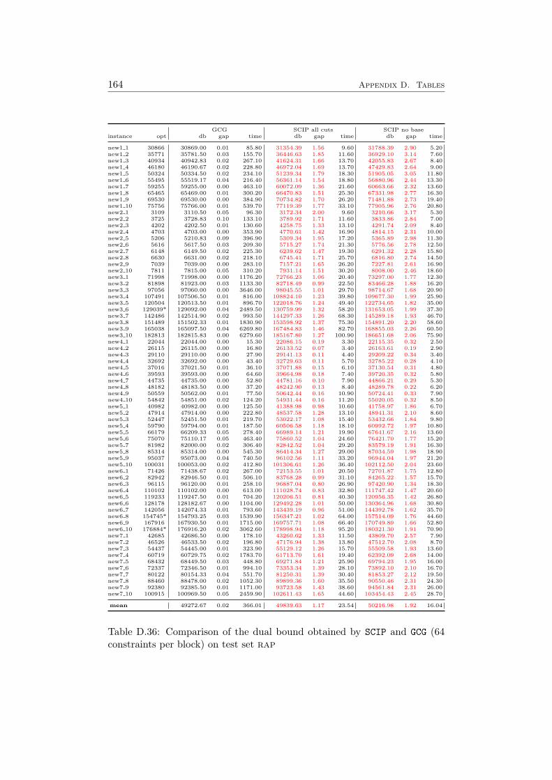
164 Appendix D. Tables
GCG SCIP all cuts SCIP no baseinstance opt db gap time db gap time db gap time
new1 1 30866 30869.00 0.01 85.80 31354.39 1.56 9.60 31788.39 2.90 5.20new1 2 35771 35781.50 0.03 155.70 36446.63 1.85 11.60 36929.10 3.14 7.60new1 3 40934 40942.83 0.02 267.10 41624.31 1.66 13.70 42055.83 2.67 8.40new1 4 46180 46190.67 0.02 228.80 46972.04 1.69 13.70 47429.83 2.64 9.00new1 5 50324 50334.50 0.02 234.10 51239.34 1.79 18.30 51905.05 3.05 11.80new1 6 55495 55519.17 0.04 216.40 56361.14 1.54 18.80 56880.96 2.44 13.30new1 7 59255 59255.00 0.00 463.10 60072.09 1.36 21.60 60663.66 2.32 13.60new1 8 65465 65469.00 0.01 300.20 66470.83 1.51 25.30 67331.98 2.77 16.30new1 9 69530 69530.00 0.00 384.90 70734.82 1.70 26.20 71481.88 2.73 19.40new1 10 75756 75766.00 0.01 539.70 77119.39 1.77 33.10 77905.96 2.76 20.80new2 1 3109 3110.50 0.05 96.30 3172.34 2.00 9.60 3210.66 3.17 5.30new2 2 3725 3728.83 0.10 133.10 3789.92 1.71 11.60 3833.86 2.84 7.00new2 3 4202 4202.50 0.01 130.60 4258.75 1.33 13.10 4291.74 2.09 8.40new2 4 4703 4703.00 0.00 353.90 4770.61 1.42 16.90 4814.15 2.31 10.00new2 5 5206 5210.83 0.09 396.90 5309.34 1.95 17.20 5365.89 2.98 11.30new2 6 5616 5617.50 0.03 209.30 5715.27 1.74 21.30 5776.56 2.78 12.50new2 7 6148 6149.50 0.02 225.30 6239.62 1.47 19.30 6291.32 2.28 15.80new2 8 6630 6631.00 0.02 218.10 6745.41 1.71 25.70 6816.80 2.74 14.50new2 9 7039 7039.00 0.00 283.10 7157.21 1.65 26.20 7227.81 2.61 16.90new2 10 7811 7815.00 0.05 310.20 7931.14 1.51 30.20 8008.00 2.46 18.60new3 1 71998 71998.00 0.00 1176.20 72766.23 1.06 20.40 73297.00 1.77 12.30new3 2 81898 81923.00 0.03 1133.30 82718.49 0.99 22.50 83466.28 1.88 16.20new3 3 97056 97060.00 0.00 3646.00 98045.55 1.01 29.70 98714.67 1.68 20.90new3 4 107491 107506.50 0.01 816.00 108824.10 1.23 39.80 109677.30 1.99 25.90new3 5 120504 120513.50 0.01 896.70 122018.76 1.24 49.40 122734.65 1.82 35.00new3 6 129039* 129092.00 0.04 2489.50 130759.99 1.32 58.20 131653.05 1.99 37.30new3 7 142486 142514.90 0.02 993.50 144297.33 1.26 68.30 145289.18 1.93 46.70new3 8 151489 151502.33 0.01 1830.90 153598.92 1.37 75.30 154891.20 2.20 58.60new3 9 165038 165097.50 0.04 6269.80 167484.83 1.46 82.70 168855.03 2.26 60.50new3 10 182813 182815.83 0.00 6279.60 185167.80 1.27 100.90 186651.68 2.06 75.90new4 1 22044 22044.00 0.00 15.30 22086.15 0.19 3.30 22115.35 0.32 2.50new4 2 26115 26115.00 0.00 16.80 26133.52 0.07 3.40 26163.61 0.19 2.90new4 3 29110 29110.00 0.00 27.90 29141.13 0.11 4.40 29209.22 0.34 3.40new4 4 32692 32692.00 0.00 43.40 32729.63 0.11 5.70 32785.22 0.28 4.10new4 5 37016 37021.50 0.01 36.10 37071.88 0.15 6.10 37130.54 0.31 4.80new4 6 39593 39593.00 0.00 64.60 39664.98 0.18 7.40 39720.35 0.32 5.80new4 7 44735 44735.00 0.00 52.80 44781.16 0.10 7.90 44866.21 0.29 5.30new4 8 48182 48183.50 0.00 37.20 48242.90 0.13 8.40 48289.78 0.22 6.20new4 9 50559 50562.00 0.01 77.50 50642.44 0.16 10.90 50724.41 0.33 7.90new4 10 54842 54851.00 0.02 124.20 54931.44 0.16 11.20 55020.05 0.32 8.50new5 1 40982 40982.00 0.00 125.50 41388.98 0.98 10.60 41758.97 1.86 6.70new5 2 47914 47914.00 0.00 222.80 48537.58 1.28 13.10 48941.31 2.10 8.60new5 3 52447 52451.50 0.01 219.70 53022.17 1.08 15.40 53432.66 1.84 9.80new5 4 59790 59794.00 0.01 187.50 60506.58 1.18 18.10 60992.72 1.97 10.80new5 5 66179 66209.33 0.05 278.40 66989.14 1.21 19.90 67641.67 2.16 13.60new5 6 75070 75110.17 0.05 463.40 75860.52 1.04 24.60 76421.70 1.77 15.20new5 7 81982 82000.00 0.02 306.40 82842.52 1.04 29.20 83579.19 1.91 16.30new5 8 85314 85314.00 0.00 545.30 86414.34 1.27 29.00 87034.59 1.98 18.90new5 9 95037 95073.00 0.04 740.50 96102.56 1.11 33.20 96944.04 1.97 21.20new5 10 100031 100053.00 0.02 412.80 101306.61 1.26 36.40 102112.50 2.04 23.60new6 1 71426 71438.67 0.02 267.00 72153.55 1.01 20.50 72701.87 1.75 12.80new6 2 82942 82946.50 0.01 506.10 83768.28 0.99 31.10 84265.22 1.57 15.70new6 3 96115 96120.00 0.01 258.10 96887.04 0.80 26.90 97420.90 1.34 18.30new6 4 110102 110102.00 0.00 613.00 111028.74 0.83 32.80 111747.42 1.47 20.60new6 5 119233 119247.50 0.01 704.20 120206.51 0.81 40.30 120956.35 1.42 26.80new6 6 128178 128182.67 0.00 1104.00 129492.28 1.01 50.00 130364.96 1.68 30.80new6 7 142056 142074.33 0.01 793.60 143439.19 0.96 51.00 144392.78 1.62 35.70new6 8 154745* 154793.25 0.03 1539.90 156347.21 1.02 64.00 157514.09 1.76 44.60new6 9 167916 167930.50 0.01 1715.00 169757.71 1.08 66.40 170749.89 1.66 52.80new6 10 176884* 176916.20 0.02 3062.60 178998.94 1.18 95.20 180321.30 1.91 70.90new7 1 42685 42686.50 0.00 178.10 43260.62 1.33 11.50 43809.70 2.57 7.90new7 2 46526 46533.50 0.02 196.80 47176.94 1.38 13.80 47512.70 2.08 8.70new7 3 54437 54445.00 0.01 323.90 55129.12 1.26 15.70 55509.58 1.93 13.60new7 4 60719 60729.75 0.02 1783.70 61713.70 1.61 19.40 62392.09 2.68 14.00new7 5 68432 68449.50 0.03 448.80 69271.84 1.21 25.90 69794.23 1.95 16.00new7 6 72337 72346.50 0.01 994.10 73353.34 1.39 28.10 73892.10 2.10 16.70new7 7 80122 80154.33 0.04 551.70 81250.31 1.39 30.40 81853.27 2.12 19.50new7 8 88460 88478.00 0.02 1052.30 89899.36 1.60 35.50 90550.46 2.31 24.30new7 9 92380 92385.50 0.01 1171.00 93723.58 1.43 38.60 94561.84 2.31 26.00new7 10 100915 100969.50 0.05 2459.90 102611.43 1.65 44.60 103454.43 2.45 28.70
mean 49272.67 0.02 366.01 49839.63 1.17 23.54 50216.98 1.92 16.04
Table D.36: Comparison of the dual bound obtained by SCIP and GCG (64constraints per block) on test set rap
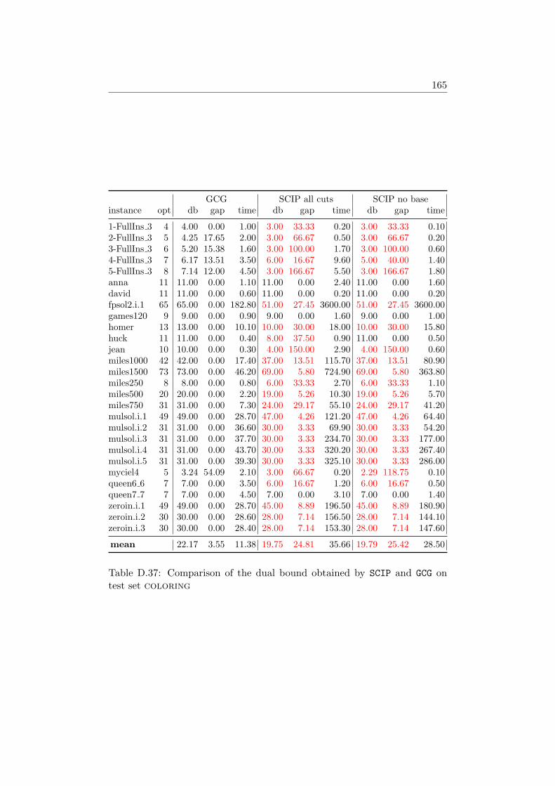
165
GCG SCIP all cuts SCIP no baseinstance opt db gap time db gap time db gap time
1-FullIns 3 4 4.00 0.00 1.00 3.00 33.33 0.20 3.00 33.33 0.102-FullIns 3 5 4.25 17.65 2.00 3.00 66.67 0.50 3.00 66.67 0.203-FullIns 3 6 5.20 15.38 1.60 3.00 100.00 1.70 3.00 100.00 0.604-FullIns 3 7 6.17 13.51 3.50 6.00 16.67 9.60 5.00 40.00 1.405-FullIns 3 8 7.14 12.00 4.50 3.00 166.67 5.50 3.00 166.67 1.80anna 11 11.00 0.00 1.10 11.00 0.00 2.40 11.00 0.00 1.60david 11 11.00 0.00 0.60 11.00 0.00 0.20 11.00 0.00 0.20fpsol2.i.1 65 65.00 0.00 182.80 51.00 27.45 3600.00 51.00 27.45 3600.00games120 9 9.00 0.00 0.90 9.00 0.00 1.60 9.00 0.00 1.00homer 13 13.00 0.00 10.10 10.00 30.00 18.00 10.00 30.00 15.80huck 11 11.00 0.00 0.40 8.00 37.50 0.90 11.00 0.00 0.50jean 10 10.00 0.00 0.30 4.00 150.00 2.90 4.00 150.00 0.60miles1000 42 42.00 0.00 17.40 37.00 13.51 115.70 37.00 13.51 80.90miles1500 73 73.00 0.00 46.20 69.00 5.80 724.90 69.00 5.80 363.80miles250 8 8.00 0.00 0.80 6.00 33.33 2.70 6.00 33.33 1.10miles500 20 20.00 0.00 2.20 19.00 5.26 10.30 19.00 5.26 5.70miles750 31 31.00 0.00 7.30 24.00 29.17 55.10 24.00 29.17 41.20mulsol.i.1 49 49.00 0.00 28.70 47.00 4.26 121.20 47.00 4.26 64.40mulsol.i.2 31 31.00 0.00 36.60 30.00 3.33 69.90 30.00 3.33 54.20mulsol.i.3 31 31.00 0.00 37.70 30.00 3.33 234.70 30.00 3.33 177.00mulsol.i.4 31 31.00 0.00 43.70 30.00 3.33 320.20 30.00 3.33 267.40mulsol.i.5 31 31.00 0.00 39.30 30.00 3.33 325.10 30.00 3.33 286.00myciel4 5 3.24 54.09 2.10 3.00 66.67 0.20 2.29 118.75 0.10queen6 6 7 7.00 0.00 3.50 6.00 16.67 1.20 6.00 16.67 0.50queen7 7 7 7.00 0.00 4.50 7.00 0.00 3.10 7.00 0.00 1.40zeroin.i.1 49 49.00 0.00 28.70 45.00 8.89 196.50 45.00 8.89 180.90zeroin.i.2 30 30.00 0.00 28.60 28.00 7.14 156.50 28.00 7.14 144.10zeroin.i.3 30 30.00 0.00 28.40 28.00 7.14 153.30 28.00 7.14 147.60
mean 22.17 3.55 11.38 19.75 24.81 35.66 19.79 25.42 28.50
Table D.37: Comparison of the dual bound obtained by SCIP and GCG ontest set coloring
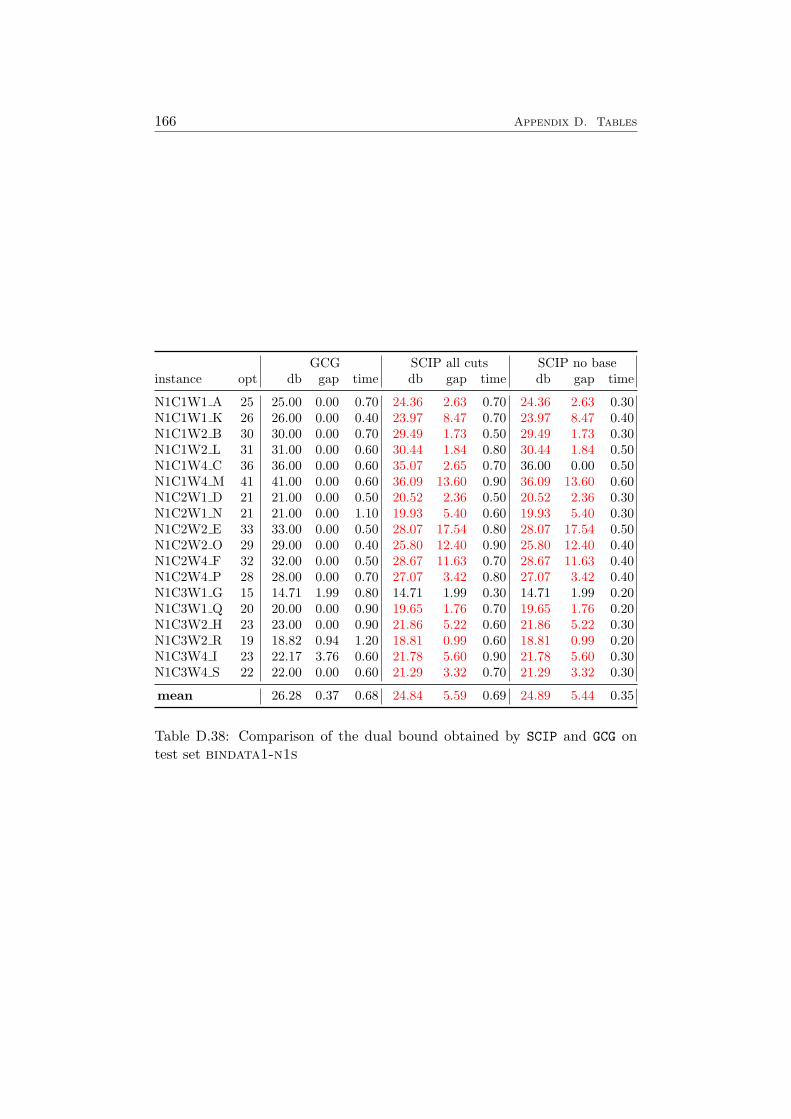
166 Appendix D. Tables
GCG SCIP all cuts SCIP no baseinstance opt db gap time db gap time db gap time
N1C1W1 A 25 25.00 0.00 0.70 24.36 2.63 0.70 24.36 2.63 0.30N1C1W1 K 26 26.00 0.00 0.40 23.97 8.47 0.70 23.97 8.47 0.40N1C1W2 B 30 30.00 0.00 0.70 29.49 1.73 0.50 29.49 1.73 0.30N1C1W2 L 31 31.00 0.00 0.60 30.44 1.84 0.80 30.44 1.84 0.50N1C1W4 C 36 36.00 0.00 0.60 35.07 2.65 0.70 36.00 0.00 0.50N1C1W4 M 41 41.00 0.00 0.60 36.09 13.60 0.90 36.09 13.60 0.60N1C2W1 D 21 21.00 0.00 0.50 20.52 2.36 0.50 20.52 2.36 0.30N1C2W1 N 21 21.00 0.00 1.10 19.93 5.40 0.60 19.93 5.40 0.30N1C2W2 E 33 33.00 0.00 0.50 28.07 17.54 0.80 28.07 17.54 0.50N1C2W2 O 29 29.00 0.00 0.40 25.80 12.40 0.90 25.80 12.40 0.40N1C2W4 F 32 32.00 0.00 0.50 28.67 11.63 0.70 28.67 11.63 0.40N1C2W4 P 28 28.00 0.00 0.70 27.07 3.42 0.80 27.07 3.42 0.40N1C3W1 G 15 14.71 1.99 0.80 14.71 1.99 0.30 14.71 1.99 0.20N1C3W1 Q 20 20.00 0.00 0.90 19.65 1.76 0.70 19.65 1.76 0.20N1C3W2 H 23 23.00 0.00 0.90 21.86 5.22 0.60 21.86 5.22 0.30N1C3W2 R 19 18.82 0.94 1.20 18.81 0.99 0.60 18.81 0.99 0.20N1C3W4 I 23 22.17 3.76 0.60 21.78 5.60 0.90 21.78 5.60 0.30N1C3W4 S 22 22.00 0.00 0.60 21.29 3.32 0.70 21.29 3.32 0.30
mean 26.28 0.37 0.68 24.84 5.59 0.69 24.89 5.44 0.35
Table D.38: Comparison of the dual bound obtained by SCIP and GCG ontest set bindata1-n1s
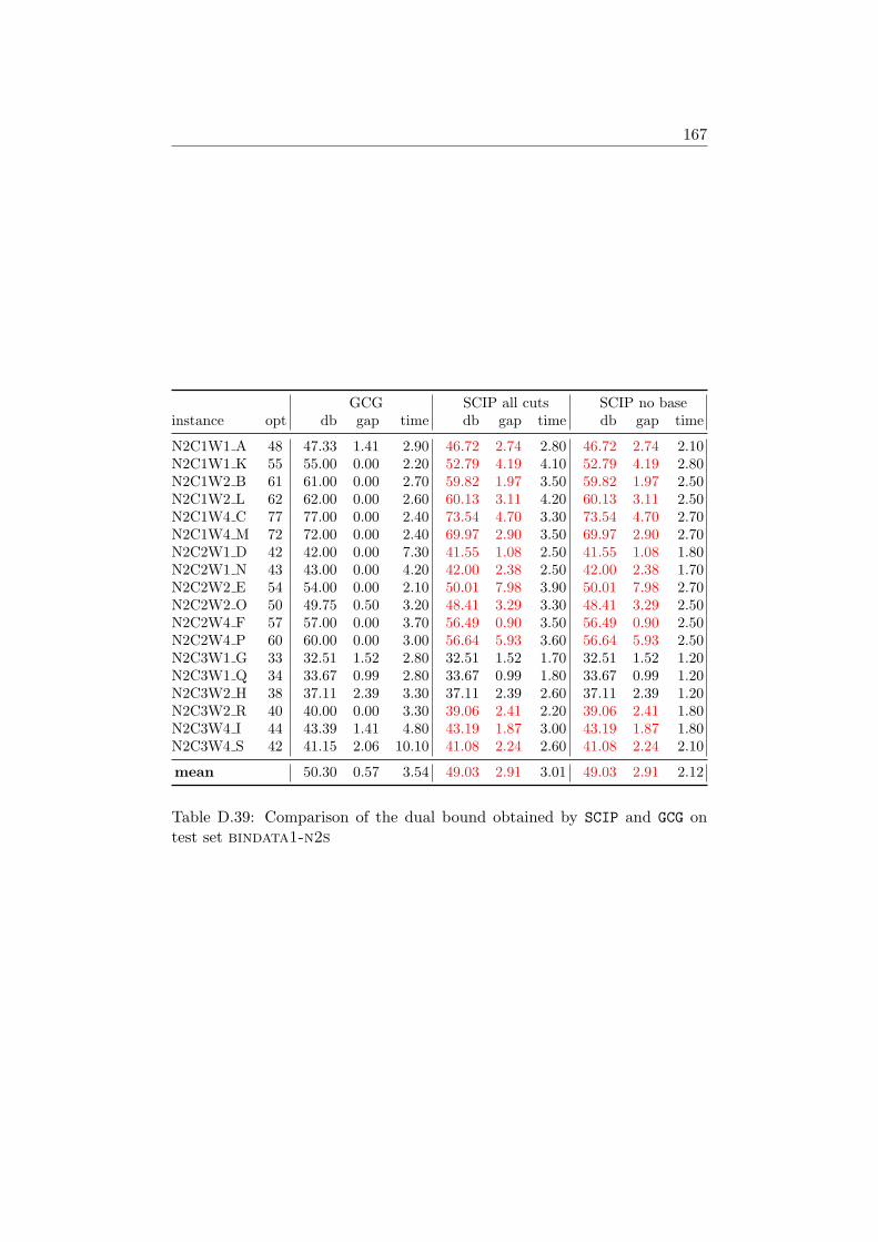
167
GCG SCIP all cuts SCIP no baseinstance opt db gap time db gap time db gap time
N2C1W1 A 48 47.33 1.41 2.90 46.72 2.74 2.80 46.72 2.74 2.10N2C1W1 K 55 55.00 0.00 2.20 52.79 4.19 4.10 52.79 4.19 2.80N2C1W2 B 61 61.00 0.00 2.70 59.82 1.97 3.50 59.82 1.97 2.50N2C1W2 L 62 62.00 0.00 2.60 60.13 3.11 4.20 60.13 3.11 2.50N2C1W4 C 77 77.00 0.00 2.40 73.54 4.70 3.30 73.54 4.70 2.70N2C1W4 M 72 72.00 0.00 2.40 69.97 2.90 3.50 69.97 2.90 2.70N2C2W1 D 42 42.00 0.00 7.30 41.55 1.08 2.50 41.55 1.08 1.80N2C2W1 N 43 43.00 0.00 4.20 42.00 2.38 2.50 42.00 2.38 1.70N2C2W2 E 54 54.00 0.00 2.10 50.01 7.98 3.90 50.01 7.98 2.70N2C2W2 O 50 49.75 0.50 3.20 48.41 3.29 3.30 48.41 3.29 2.50N2C2W4 F 57 57.00 0.00 3.70 56.49 0.90 3.50 56.49 0.90 2.50N2C2W4 P 60 60.00 0.00 3.00 56.64 5.93 3.60 56.64 5.93 2.50N2C3W1 G 33 32.51 1.52 2.80 32.51 1.52 1.70 32.51 1.52 1.20N2C3W1 Q 34 33.67 0.99 2.80 33.67 0.99 1.80 33.67 0.99 1.20N2C3W2 H 38 37.11 2.39 3.30 37.11 2.39 2.60 37.11 2.39 1.20N2C3W2 R 40 40.00 0.00 3.30 39.06 2.41 2.20 39.06 2.41 1.80N2C3W4 I 44 43.39 1.41 4.80 43.19 1.87 3.00 43.19 1.87 1.80N2C3W4 S 42 41.15 2.06 10.10 41.08 2.24 2.60 41.08 2.24 2.10
mean 50.30 0.57 3.54 49.03 2.91 3.01 49.03 2.91 2.12
Table D.39: Comparison of the dual bound obtained by SCIP and GCG ontest set bindata1-n2s

168 Appendix D. Tables
GCG SCIP all cuts SCIP no baseinstance opt db gap time db gap time db gap time
N3C1W1 A 105 105.00 0.00 12.40 100.88 4.08 22.50 100.88 4.08 18.10N3C1W1 K 102 102.00 0.00 13.10 99.51 2.50 20.20 99.51 2.50 17.10N3C1W2 B 126 126.00 0.00 13.20 118.37 6.45 29.00 118.37 6.45 24.50N3C1W2 L 136 136.00 0.00 15.40 131.23 3.63 30.90 131.23 3.63 26.50N3C1W4 C 146 146.00 0.00 18.10 142.66 2.34 31.40 142.66 2.34 25.10N3C1W4 M 149 149.00 0.00 17.90 144.27 3.28 31.40 144.27 3.28 26.20N3C2W1 D 85 85.00 0.00 9.60 83.19 2.17 14.90 83.19 2.17 12.10N3C2W1 N 91 91.00 0.00 10.40 86.70 4.96 19.60 86.70 4.96 16.00N3C2W2 E 116 116.00 0.00 13.50 107.22 8.18 26.90 107.22 8.18 21.20N3C2W2 O 107 107.00 0.00 13.30 101.40 5.52 23.90 101.40 5.52 20.60N3C2W4 F 115 115.00 0.00 20.90 110.63 3.95 25.30 110.63 3.95 20.60N3C2W4 P 122 122.00 0.00 18.50 115.76 5.39 27.60 115.76 5.39 22.70N3C3W1 G 65 64.16 1.31 10.30 64.16 1.31 9.70 64.16 1.31 8.40N3C3W1 Q 73 72.61 0.54 11.80 72.61 0.54 13.20 72.61 0.54 10.30N3C3W2 H 82 81.85 0.19 33.80 81.82 0.22 17.90 81.82 0.22 12.50N3C3W2 R 79 78.51 0.63 14.20 78.51 0.63 14.60 78.51 0.63 12.40N3C3W4 I 92 91.25 0.82 14.00 90.09 2.12 20.60 90.09 2.12 16.90N3C3W4 S 84 83.08 1.11 32.70 83.03 1.16 16.50 83.03 1.16 13.00
mean 103.48 0.25 15.59 100.25 3.22 21.31 100.25 3.22 17.44
Table D.40: Comparison of the dual bound obtained by SCIP and GCG ontest set bindata1-n3s

169
default 20 vars 10% no limitinstance vars gap nodes time vars gap nodes time vars gap nodes time vars gap nodes time
p550-1 3491 0.0 32 11.9 4009 0.0 24 13.0 3274 0.0 21 14.6 3117 0.0 23 10.8p550-3 3526 0.0 3 6.5 3526 0.0 3 6.5 3531 0.0 3 8.8 4030 0.0 3 6.6p550-5 3876 0.0 1 7.2 3876 0.0 1 7.2 3876 0.0 1 7.1 3639 0.0 1 5.6p550-7 3735 0.0 15 13.2 3737 0.0 16 14.0 3844 0.0 21 30.6 3933 0.0 15 13.7p550-9 2925 0.0 9 6.1 2925 0.0 9 6.1 2929 0.0 5 6.6 3118 0.0 7 6.7p1250-1 2168 0.0 173 18.8 2090 0.0 157 17.0 1956 0.0 141 14.2 2044 0.0 178 17.7p1250-3 1825 0.0 155 18.7 1824 0.0 155 18.8 1810 0.0 137 17.2 1802 0.0 69 10.2p1250-5 2204 0.0 68 11.7 2199 0.0 68 11.5 2324 0.0 134 21.2 2340 0.0 87 15.8p1250-7 3019 0.0 1514 174.3 2714 0.0 1332 167.7 2677 0.0 1676 188.4 4041 0.0 1921 215.6p1250-9 2085 0.0 138 36.9 2030 0.0 143 31.4 1982 0.0 123 29.1 2092 0.0 97 24.0p1650-1 1484 0.0 8 2.6 1487 0.0 8 2.7 1469 0.0 8 2.6 1526 0.0 5 2.3p1650-3 1418 0.0 13 2.8 1418 0.0 13 2.8 1434 0.0 10 3.3 1403 0.0 9 2.6p1650-5 1752 0.0 59 8.5 1761 0.0 59 8.7 1705 0.0 78 9.8 1766 0.0 99 14.4p1650-7 1325 0.0 75 9.8 1325 0.0 75 9.8 1334 0.0 81 10.2 1390 0.0 53 7.8p1650-9 1567 0.0 198 26.7 1567 0.0 198 26.7 1552 0.0 195 25.9 1847 0.0 150 22.1p2050-1 1285 0.0 38 4.5 1285 0.0 38 4.5 1272 0.0 36 4.6 1231 0.0 57 5.3p2050-3 1282 0.0 11 3.5 1282 0.0 11 3.5 1288 0.0 11 3.6 1221 0.0 12 3.2p2050-5 1262 0.0 5 2.9 1262 0.0 5 2.9 1262 0.0 5 2.8 1259 0.0 6 3.4p2050-7 1166 0.0 5 3.0 1166 0.0 5 3.0 1166 0.0 5 2.9 1181 0.0 7 3.3p2050-9 1356 0.0 343 46.3 1356 0.0 343 46.3 1320 0.0 331 44.8 1364 0.0 355 46.7
total 42k 0.0 2863 415.9 42k 0.0 2663 404.1 42k 0.0 3022 448.3 44k 0.0 3154 437.8timeouts 0/20 0/20 0/20 0/20mean 2016.4 0.0 44.9 12.8 2014.9 0.0 43.9 12.7 1983.0 0.0 45.0 13.9 2075.0 0.0 42.7 12.4
Table D.41. Impact of the reduced cost pricing setting at subsequent nodes on the performance of GCG (test set cpmp50s)
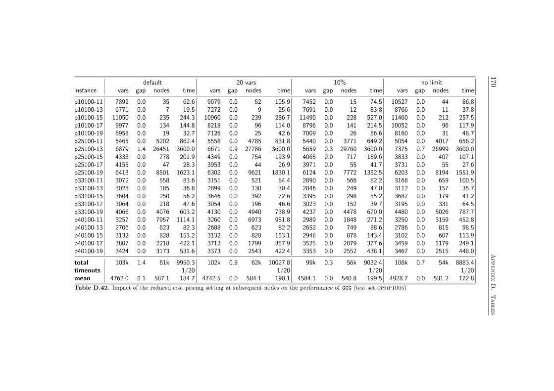
170A
ppendix
D.
Tables
default 20 vars 10% no limitinstance vars gap nodes time vars gap nodes time vars gap nodes time vars gap nodes time
p10100-11 7892 0.0 35 62.6 9079 0.0 52 105.9 7452 0.0 15 74.5 10527 0.0 44 86.8p10100-13 6771 0.0 7 19.5 7272 0.0 9 25.6 7691 0.0 12 83.8 8766 0.0 11 37.8p10100-15 11050 0.0 235 244.3 10960 0.0 239 286.7 11490 0.0 228 527.0 11460 0.0 212 257.5p10100-17 9977 0.0 134 144.8 8218 0.0 96 114.0 8796 0.0 141 214.5 10052 0.0 96 117.9p10100-19 6958 0.0 19 32.7 7126 0.0 25 42.6 7009 0.0 26 86.6 8160 0.0 31 48.7p25100-11 5465 0.0 5202 862.4 5558 0.0 4785 831.8 5440 0.0 3771 649.2 5054 0.0 4017 656.2p25100-13 6879 1.4 26451 3600.0 6671 0.9 27786 3600.0 5659 0.3 29760 3600.0 7375 0.7 26999 3600.0p25100-15 4333 0.0 778 201.9 4349 0.0 754 193.9 4065 0.0 717 189.6 3833 0.0 407 107.1p25100-17 4155 0.0 47 28.3 3953 0.0 44 26.9 3971 0.0 55 41.7 3731 0.0 55 27.6p25100-19 6413 0.0 8501 1623.1 6302 0.0 9621 1830.1 6124 0.0 7772 1352.5 6203 0.0 8194 1551.9p33100-11 3072 0.0 558 83.6 3151 0.0 521 84.4 2890 0.0 566 82.2 3168 0.0 659 100.5p33100-13 3028 0.0 185 36.8 2899 0.0 130 30.4 2846 0.0 249 47.0 3112 0.0 157 35.7p33100-15 3604 0.0 250 56.2 3646 0.0 392 72.6 3395 0.0 298 55.2 3687 0.0 179 41.2p33100-17 3064 0.0 218 47.6 3054 0.0 196 46.6 3023 0.0 152 39.7 3195 0.0 331 64.5p33100-19 4066 0.0 4076 603.2 4130 0.0 4940 738.9 4237 0.0 4478 670.0 4480 0.0 5026 787.7p40100-11 3257 0.0 7957 1114.1 3260 0.0 6973 981.8 2989 0.0 1848 271.2 3250 0.0 3159 452.8p40100-13 2706 0.0 623 82.3 2688 0.0 623 82.2 2652 0.0 749 88.6 2786 0.0 815 98.5p40100-15 3132 0.0 828 153.2 3132 0.0 828 153.1 2948 0.0 878 143.4 3102 0.0 607 113.9p40100-17 3807 0.0 2218 422.1 3712 0.0 1799 357.9 3525 0.0 2079 377.6 3459 0.0 1179 249.1p40100-19 3424 0.0 3173 531.6 3373 0.0 2543 422.4 3353 0.0 2552 438.1 3467 0.0 2515 448.0
total 103k 1.4 61k 9950.3 102k 0.9 62k 10027.8 99k 0.3 56k 9032.4 108k 0.7 54k 8883.4timeouts 1/20 1/20 1/20 1/20mean 4762.0 0.1 587.1 184.7 4742.5 0.0 584.1 190.1 4584.1 0.0 540.8 199.5 4928.7 0.0 531.2 172.8
Table D.42. Impact of the reduced cost pricing setting at subsequent nodes on the performance of GCG (test set cpmp100s)
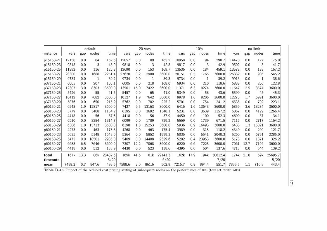
171
default 20 vars 10% no limitinstance vars gap nodes time vars gap nodes time vars gap nodes time vars gap nodes time
p15150-21 12150 0.0 84 162.6 12057 0.0 89 165.2 10958 0.0 94 290.7 14470 0.0 127 175.0p15150-23 9818 0.0 3 43.0 9818 0.0 3 42.8 9817 0.0 3 42.9 9502 0.0 3 41.7p15150-25 11392 0.0 116 125.3 12690 0.0 153 169.7 13536 0.0 184 459.1 13578 0.0 138 167.2p15150-27 28300 0.0 1688 2251.4 27620 0.2 2980 3600.0 28151 0.5 1765 3600.0 26332 0.0 906 1545.2p15150-29 9734 0.0 1 39.2 9734 0.0 1 39.3 9734 0.0 1 39.2 9913 0.0 1 38.6p37150-21 6005 0.0 207 105.1 6005 0.0 218 108.0 5934 0.0 210 118.6 6838 0.0 206 122.8p37150-23 12307 3.0 8303 3600.0 13501 16.0 7422 3600.0 11371 6.3 9274 3600.0 11647 2.5 8574 3600.0p37150-25 5426 0.0 55 41.5 5457 0.0 65 41.0 5349 0.0 58 43.6 5599 0.0 45 45.3p37150-27 10412 0.9 7682 3600.0 10127 1.9 7642 3600.0 9978 1.6 8206 3600.0 12273 1.7 6991 3600.0p37150-29 5876 0.0 650 215.9 5762 0.0 702 225.2 5701 0.0 754 241.2 6535 0.0 702 223.1p50150-21 6543 1.9 12817 3600.0 7427 9.5 13163 3600.0 6416 1.6 13643 3600.0 6859 3.6 13234 3600.0p50150-23 5779 0.0 3408 1154.2 6195 0.0 3692 1340.1 5231 0.0 3639 1157.2 6067 0.0 4129 1266.4p50150-25 4418 0.0 56 37.5 4418 0.0 56 37.9 4450 0.0 100 52.3 4699 0.0 37 34.1p50150-27 6510 0.0 3284 1314.7 6099 0.0 1789 729.2 5569 0.0 1739 671.5 7115 0.0 2717 1164.2p50150-29 6386 1.0 15713 3600.0 6198 1.8 15253 3600.0 5936 0.9 16493 3600.0 6433 1.3 15821 3600.0p60150-21 4273 0.0 463 175.3 4268 0.0 463 175.4 3989 0.0 315 118.2 4349 0.0 290 121.7p60150-23 5635 0.0 5148 1648.0 5364 0.0 5852 1999.3 5036 0.0 6541 2040.3 5260 0.0 6791 2285.0p60150-25 5475 0.0 18501 2985.0 5409 0.0 14488 2329.6 5202 0.4 23953 3600.0 5173 0.0 1371 326.2p60150-27 6688 6.5 7646 3600.0 7307 12.2 7068 3600.0 6220 6.6 7225 3600.0 7061 12.7 7104 3600.0p60150-29 4418 0.0 512 133.9 4430 0.0 523 138.6 4395 0.0 504 137.6 4718 0.0 544 139.2
total 167k 13.3 86k 28432.6 169k 41.6 81k 29141.3 162k 17.9 94k 30612.4 174k 21.8 69k 25695.7timeouts 5/20 6/20 7/20 5/20mean 7489.2 0.7 847.6 493.5 7588.6 2.0 861.6 502.9 7216.7 0.9 894.4 551.7 7835.5 1.1 716.3 443.4
Table D.43. Impact of the reduced cost pricing setting at subsequent nodes on the performance of GCG (test set cpmp150s)
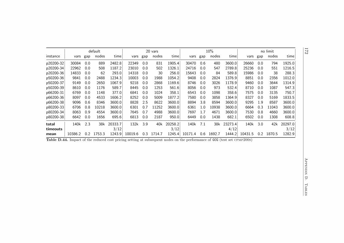
172A
ppendix
D.
Tables
default 20 vars 10% no limitinstance vars gap nodes time vars gap nodes time vars gap nodes time vars gap nodes time
p20200-32 30084 0.0 889 2482.8 22349 0.0 831 1905.4 30470 0.6 480 3600.0 26660 0.0 794 1925.0p20200-34 22962 0.0 508 1187.2 23010 0.0 502 1326.1 24716 0.0 547 2789.8 25236 0.0 551 1216.5p20200-36 14833 0.0 62 293.0 14318 0.0 30 256.0 15643 0.0 84 589.8 15986 0.0 38 288.3p50200-36 9841 0.0 2488 1234.3 10003 0.0 1988 1054.2 9408 0.0 2824 1376.9 8851 0.0 2356 1012.0p50200-37 9149 0.0 2650 1067.9 9218 0.0 2868 1169.6 8746 0.0 3026 1178.9 9460 0.0 3644 1314.9p50200-39 8610 0.0 1176 589.7 8445 0.0 1253 561.6 8056 0.0 973 532.4 8710 0.0 1087 547.3p66200-31 6769 0.0 1148 377.0 6841 0.0 1024 358.1 6543 0.0 1098 358.6 7575 0.0 3135 750.7p66200-36 8097 0.0 4533 1606.2 8252 0.0 5009 1877.2 7580 0.0 3858 1364.9 8327 0.0 5169 1833.5p66200-38 9096 0.6 8346 3600.0 8828 2.5 8622 3600.0 8894 3.8 8594 3600.0 9295 1.9 8587 3600.0p80200-33 6706 0.8 10218 3600.0 6301 0.7 11252 3600.0 6361 1.0 10938 3600.0 6664 0.3 11043 3600.0p80200-34 8063 0.9 4554 3600.0 7645 0.7 4988 3600.0 7697 1.7 4671 3600.0 7530 0.8 4660 3600.0p80200-38 6642 0.0 1656 695.6 6813 0.0 2187 950.0 6449 0.0 1438 682.1 6502 0.0 1308 608.8
total 140k 2.3 38k 20333.7 132k 3.9 40k 20258.2 140k 7.1 38k 23273.4 140k 3.0 42k 20297.0timeouts 3/12 3/12 4/12 3/12mean 10386.2 0.2 1753.3 1243.9 10019.6 0.3 1714.7 1245.4 10171.4 0.6 1692.7 1444.2 10431.5 0.2 1870.5 1282.9
Table D.44. Impact of the reduced cost pricing setting at subsequent nodes on the performance of GCG (test set cpmp200s)

173
default 20 vars 10% no limitinstance vars gap nodes time vars gap nodes time vars gap nodes time vars gap nodes time
new1 2 32 3073 0.0 119 979.6 3073 0.0 119 975.8 3094 0.0 119 838.8 3766 0.0 119 973.6new1 6 32 3690 0.0 17 468.5 3690 0.0 17 467.3 3693 0.0 21 424.3 4570 0.0 17 410.0new1 10 32 6344 0.0 35 1085.1 6344 0.0 35 1079.5 6342 0.0 35 1025.9 7437 0.0 39 912.5new2 1 32 2102 0.0 7 109.5 2102 0.0 7 109.2 2104 0.0 7 105.7 2370 0.0 7 81.5new2 3 32 2365 0.0 23 299.5 2365 0.0 23 298.4 2375 0.0 23 261.8 2706 0.0 23 243.9new2 7 32 3576 0.0 36 642.2 3576 0.0 36 640.8 3552 0.0 21 445.3 4149 0.0 97 1415.3new3 1 32 3875 0.0 31 1205.1 3747 0.0 27 1163.5 3890 0.0 27 996.7 4151 0.0 35 1447.3new3 4 32 5235 0.0 39 2596.2 5235 0.0 39 2586.8 5237 0.0 37 2487.1 5915 0.0 37 2229.7new3 5 32 6261 0.0 33 1937.4 6257 0.0 33 1946.3 6262 0.0 33 1747.4 7315 0.0 29 1852.4new4 1 32 833 0.0 1 26.1 833 0.0 1 26.0 833 0.0 1 26.1 952 0.0 1 26.1new4 5 32 1502 0.0 13 86.4 1502 0.0 13 85.6 1502 0.0 13 74.7 1662 0.0 13 90.2new4 10 32 2474 0.0 3 61.0 2474 0.0 3 60.5 2474 0.0 3 60.7 2696 0.0 5 92.9new5 2 32 3182 0.0 11 248.6 3182 0.0 11 247.6 3179 0.0 11 225.1 3906 0.0 11 290.2new5 7 32 5601 0.0 133 2008.2 5601 0.0 133 1998.6 5638 0.0 135 2027.1 6865 0.0 193 2916.1new5 10 32 6982 0.0 85 2109.2 6982 0.0 85 2103.0 6989 0.0 74 1682.2 8466 0.0 37 1207.5new6 1 32 3604 0.0 25 692.2 3604 0.0 25 689.6 3595 0.0 25 576.7 4046 0.0 21 630.1new6 2 32 4983 0.0 7 518.3 4983 0.0 7 516.9 4991 0.0 7 482.1 5996 0.0 7 569.9new6 5 32 6962 0.0 29 1546.7 6957 0.0 29 1541.1 6956 0.0 29 1405.6 8368 0.0 47 2377.4new7 1 32 3300 0.0 58 614.3 3300 0.0 58 613.7 3312 0.0 55 519.4 4124 0.0 52 632.6new7 4 32 5582 0.0 25 665.2 5582 0.0 25 663.3 5582 0.0 25 614.0 6702 0.0 62 1235.0new7 9 32 7228 0.0 31 1051.1 7228 0.0 31 1050.4 7229 0.0 31 1048.2 8776 0.0 19 1004.3
total 88k 0.0 761 18950.4 88k 0.0 757 18863.9 88k 0.0 732 17074.9 104k 0.0 871 20638.5timeouts 0/21 0/21 0/21 0/21mean 3862.2 0.0 26.8 551.5 3855.8 0.0 26.6 548.9 3865.6 0.0 25.8 495.7 4520.7 0.0 28.9 590.0
Table D.45. Impact of the reduced cost pricing setting at subsequent nodes on the performance of GCG (test set rap32s)
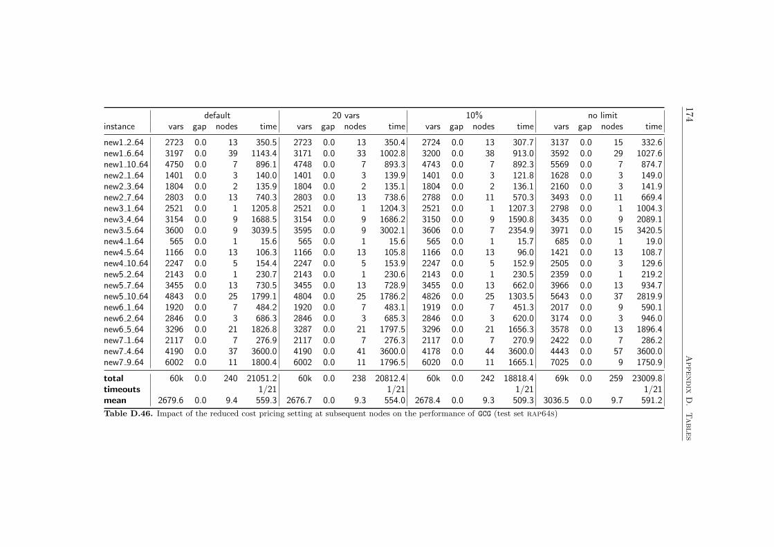
174A
ppendix
D.
Tables
default 20 vars 10% no limitinstance vars gap nodes time vars gap nodes time vars gap nodes time vars gap nodes time
new1 2 64 2723 0.0 13 350.5 2723 0.0 13 350.4 2724 0.0 13 307.7 3137 0.0 15 332.6new1 6 64 3197 0.0 39 1143.4 3171 0.0 33 1002.8 3200 0.0 38 913.0 3592 0.0 29 1027.6new1 10 64 4750 0.0 7 896.1 4748 0.0 7 893.3 4743 0.0 7 892.3 5569 0.0 7 874.7new2 1 64 1401 0.0 3 140.0 1401 0.0 3 139.9 1401 0.0 3 121.8 1628 0.0 3 149.0new2 3 64 1804 0.0 2 135.9 1804 0.0 2 135.1 1804 0.0 2 136.1 2160 0.0 3 141.9new2 7 64 2803 0.0 13 740.3 2803 0.0 13 738.6 2788 0.0 11 570.3 3493 0.0 11 669.4new3 1 64 2521 0.0 1 1205.8 2521 0.0 1 1204.3 2521 0.0 1 1207.3 2798 0.0 1 1004.3new3 4 64 3154 0.0 9 1688.5 3154 0.0 9 1686.2 3150 0.0 9 1590.8 3435 0.0 9 2089.1new3 5 64 3600 0.0 9 3039.5 3595 0.0 9 3002.1 3606 0.0 7 2354.9 3971 0.0 15 3420.5new4 1 64 565 0.0 1 15.6 565 0.0 1 15.6 565 0.0 1 15.7 685 0.0 1 19.0new4 5 64 1166 0.0 13 106.3 1166 0.0 13 105.8 1166 0.0 13 96.0 1421 0.0 13 108.7new4 10 64 2247 0.0 5 154.4 2247 0.0 5 153.9 2247 0.0 5 152.9 2505 0.0 3 129.6new5 2 64 2143 0.0 1 230.7 2143 0.0 1 230.6 2143 0.0 1 230.5 2359 0.0 1 219.2new5 7 64 3455 0.0 13 730.5 3455 0.0 13 728.9 3455 0.0 13 662.0 3966 0.0 13 934.7new5 10 64 4843 0.0 25 1799.1 4804 0.0 25 1786.2 4826 0.0 25 1303.5 5643 0.0 37 2819.9new6 1 64 1920 0.0 7 484.2 1920 0.0 7 483.1 1919 0.0 7 451.3 2017 0.0 9 590.1new6 2 64 2846 0.0 3 686.3 2846 0.0 3 685.3 2846 0.0 3 620.0 3174 0.0 3 946.0new6 5 64 3296 0.0 21 1826.8 3287 0.0 21 1797.5 3296 0.0 21 1656.3 3578 0.0 13 1896.4new7 1 64 2117 0.0 7 276.9 2117 0.0 7 276.3 2117 0.0 7 270.9 2422 0.0 7 286.2new7 4 64 4190 0.0 37 3600.0 4190 0.0 41 3600.0 4178 0.0 44 3600.0 4443 0.0 57 3600.0new7 9 64 6002 0.0 11 1800.4 6002 0.0 11 1796.5 6020 0.0 11 1665.1 7025 0.0 9 1750.9
total 60k 0.0 240 21051.2 60k 0.0 238 20812.4 60k 0.0 242 18818.4 69k 0.0 259 23009.8timeouts 1/21 1/21 1/21 1/21mean 2679.6 0.0 9.4 559.3 2676.7 0.0 9.3 554.0 2678.4 0.0 9.3 509.3 3036.5 0.0 9.7 591.2
Table D.46. Impact of the reduced cost pricing setting at subsequent nodes on the performance of GCG (test set rap64s)
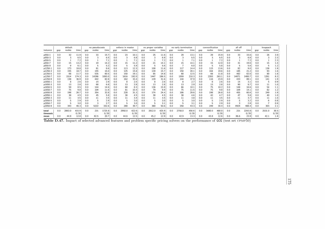
175
default no pseudocosts enforce in master no proper variables no early termination convexification all off knapsackinstance gap nodes time gap nodes time gap nodes time gap nodes time gap nodes time gap nodes time gap nodes time gap nodes time
p550-1 0.0 32 11.9 0.0 33 15.7 0.0 23 10.1 0.0 25 11.6 0.0 29 13.1 0.0 29 15.9 0.0 33 15.6 0.0 26 3.9p550-3 0.0 3 6.5 0.0 3 6.5 0.0 3 6.8 0.0 3 6.9 0.0 3 6.5 0.0 3 6.5 0.0 3 6.8 0.0 3 2.3p550-5 0.0 1 7.2 0.0 1 7.1 0.0 1 7.1 0.0 1 7.2 0.0 1 7.1 0.0 1 7.2 0.0 1 7.2 0.0 1 2.3p550-7 0.0 15 13.2 0.0 19 14.2 0.0 15 11.2 0.0 21 14.1 0.0 15 14.1 0.0 15 12.0 0.0 31 19.6 0.0 15 1.4p550-9 0.0 9 6.1 0.0 5 5.2 0.0 5 5.9 0.0 5 5.6 0.0 7 6.0 0.0 5 5.8 0.0 5 5.6 0.0 5 1.2p1250-1 0.0 173 18.8 0.0 81 8.6 0.0 113 12.3 0.0 108 11.6 0.0 117 14.4 0.0 115 13.6 0.0 82 9.0 0.0 138 1.9p1250-3 0.0 155 18.7 0.0 155 16.0 0.0 125 15.8 0.0 139 15.7 0.0 150 20.1 0.0 164 19.6 0.0 185 21.2 0.0 93 1.6p1250-5 0.0 68 11.7 0.0 535 60.5 0.0 150 19.1 0.0 85 14.8 0.0 68 12.5 0.0 68 11.8 0.0 482 62.0 0.0 80 1.8p1250-7 0.0 1514 174.3 0.0 14286 1093.0 0.0 1616 192.0 0.0 1447 186.5 0.0 1559 210.3 0.0 2283 263.1 0.0 14071 1400.7 0.0 1261 8.3p1250-9 0.0 138 36.9 0.0 442 82.8 0.0 162 33.4 0.0 129 31.6 0.0 144 37.9 0.0 116 23.9 0.0 433 89.1 0.0 141 1.9p1650-1 0.0 8 2.6 0.0 14 2.9 0.0 8 2.5 0.0 8 2.6 0.0 8 2.7 0.0 8 2.6 0.0 14 3.1 0.0 5 0.9p1650-3 0.0 13 2.8 0.0 68 6.8 0.0 13 2.8 0.0 13 2.8 0.0 13 2.9 0.0 13 2.8 0.0 90 8.7 0.0 11 1.0p1650-5 0.0 59 8.5 0.0 144 14.6 0.0 60 8.3 0.0 136 15.9 0.0 66 10.1 0.0 75 10.2 0.0 148 16.6 0.0 54 1.1p1650-7 0.0 75 9.8 0.0 109 11.6 0.0 81 10.4 0.0 79 9.9 0.0 75 11.5 0.0 75 9.8 0.0 109 14.1 0.0 82 1.2p1650-9 0.0 198 26.7 0.0 354 32.8 0.0 228 31.3 0.0 174 24.4 0.0 186 29.6 0.0 198 26.8 0.0 455 60.6 0.0 249 1.9p2050-1 0.0 38 4.5 0.0 45 5.8 0.0 38 4.5 0.0 38 4.5 0.0 38 4.6 0.0 42 4.7 0.0 47 5.8 0.0 40 1.0p2050-3 0.0 11 3.5 0.0 11 3.5 0.0 11 3.4 0.0 11 3.5 0.0 11 3.8 0.0 11 3.5 0.0 11 3.7 0.0 11 1.0p2050-5 0.0 5 2.9 0.0 5 2.9 0.0 5 3.0 0.0 5 3.0 0.0 5 3.0 0.0 5 2.9 0.0 5 3.2 0.0 6 0.8p2050-7 0.0 5 3.0 0.0 3 2.7 0.0 5 3.0 0.0 5 3.1 0.0 5 3.1 0.0 5 2.9 0.0 3 2.8 0.0 7 0.9p2050-9 0.0 343 46.3 0.0 5222 332.6 0.0 288 39.7 0.0 380 50.6 0.0 258 43.3 0.0 249 34.4 0.0 4924 488.4 0.0 303 2.1
total 0.0 2863.0 415.9 0.0 21k 1725.8 0.0 2950.0 422.6 0.0 2812.0 425.9 0.0 2758.0 456.6 0.0 3480.0 480.0 0.0 21k 2243.8 0.0 2531.0 38.5timeouts 0/20 0/20 0/20 0/20 0/20 0/20 0/20 0/20mean 0.0 44.9 12.8 0.0 82.5 20.7 0.0 44.6 12.5 0.0 45.2 12.9 0.0 42.9 13.3 0.0 43.8 12.6 0.0 86.6 23.9 0.0 42.1 1.8
Table D.47. Impact of selected advanced features and problem specific pricing solvers on the performance of GCG (test set cpmp50)
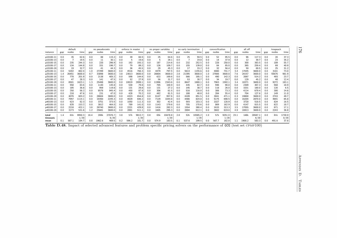
176A
ppendix
D.
Tables
default no pseudocosts enforce in master no proper variables no early termination convexification all off knapsackinstance gap nodes time gap nodes time gap nodes time gap nodes time gap nodes time gap nodes time gap nodes time gap nodes time
p10100-11 0.0 35 62.6 0.0 88 115.2 0.0 39 66.5 0.0 25 64.6 0.0 25 59.5 0.0 52 95.5 0.0 96 117.3 0.0 20 37.3p10100-13 0.0 7 19.5 0.0 11 30.1 0.0 5 19.6 0.0 5 29.1 0.0 7 19.8 0.0 14 37.9 0.0 12 39.7 0.0 23 35.2p10100-15 0.0 235 244.3 0.0 220 296.9 0.0 192 193.2 0.0 187 214.6 0.0 232 252.5 0.0 228 250.0 0.0 300 383.5 0.0 189 55.7p10100-17 0.0 134 144.8 0.0 331 196.7 0.0 79 89.2 0.0 126 109.7 0.0 155 139.0 0.0 84 85.0 0.0 365 259.4 0.0 69 40.9p10100-19 0.0 19 32.7 0.0 41 44.3 0.0 36 45.5 0.0 29 45.3 0.0 17 33.2 0.0 32 56.4 0.0 59 69.5 0.0 25 31.2p25100-11 0.0 5202 862.4 1.0 27299 3600.0 0.0 4516 766.3 0.0 4479 797.5 0.0 5614 1155.6 0.0 4080 741.7 3.4 17045 3600.0 0.0 3181 73.0p25100-13 1.4 26451 3600.0 8.7 33898 3600.0 3.8 23613 3600.0 0.8 28804 3600.0 2.8 21395 3600.0 1.0 27666 3600.0 7.6 24157 3600.0 0.0 55676 981.9p25100-15 0.0 778 201.9 0.0 2138 405.2 0.0 598 144.6 0.0 622 169.6 0.0 566 185.1 0.0 490 142.3 0.0 2067 514.2 0.0 493 23.7p25100-17 0.0 47 28.3 0.0 141 47.5 0.0 52 27.9 0.0 56 31.7 0.0 53 30.7 0.0 34 19.7 0.0 129 45.2 0.0 48 12.4p25100-19 0.0 8501 1623.1 1.3 25488 3600.0 0.0 10819 2099.1 0.0 11996 2343.6 0.0 8647 1880.1 0.0 7963 1592.1 3.4 18371 3600.0 0.0 9272 183.1p33100-11 0.0 558 83.6 0.0 1140 145.8 0.0 530 79.8 0.0 765 100.9 0.0 435 82.7 0.0 596 90.0 0.0 2309 367.3 0.0 568 18.9p33100-13 0.0 185 36.8 0.0 959 119.8 0.0 131 29.8 0.0 131 27.2 0.0 145 38.7 0.0 118 26.0 0.0 1031 180.0 0.0 120 6.5p33100-15 0.0 250 56.2 0.0 8578 945.4 0.0 450 87.8 0.0 306 61.5 0.0 516 116.8 0.0 306 73.3 0.0 4114 679.4 0.0 300 14.6p33100-17 0.0 218 47.6 0.0 231 47.0 0.0 428 70.2 0.0 482 81.5 0.0 188 48.8 0.0 284 55.4 0.0 704 127.6 0.0 149 11.0p33100-19 0.0 4076 603.2 0.6 28604 3600.0 0.0 4323 654.8 0.0 6147 957.6 0.0 4109 851.5 0.0 3041 471.1 0.3 19800 3600.0 0.0 2743 49.7p40100-11 0.0 7957 1114.1 0.0 19350 2245.3 0.0 4629 646.2 0.0 7129 1044.8 0.0 4486 824.8 0.0 5175 698.5 0.0 16204 2870.0 0.0 4691 65.8p40100-13 0.0 623 82.3 0.0 3751 373.5 0.0 1050 111.3 0.0 302 42.4 0.0 593 103.3 0.0 1027 120.9 0.0 3720 518.5 0.0 824 16.5p40100-15 0.0 828 153.2 0.0 3812 464.0 0.0 789 141.0 0.0 1143 179.6 0.0 705 170.6 0.0 869 162.9 0.0 4147 815.5 0.0 622 18.7p40100-17 0.0 2218 422.1 3.6 26740 3600.0 0.0 2221 429.8 0.0 1416 282.3 0.0 1554 380.4 0.0 1633 313.3 3.5 17055 3600.0 0.0 671 17.1p40100-19 0.0 3173 531.6 1.2 25681 3600.0 0.0 2891 511.1 0.0 1605 295.3 0.0 2694 612.1 0.0 3602 619.0 4.9 16913 3600.0 0.0 2243 36.8
total 1.4 61k 9950.3 16.4 208k 27076.7 3.8 57k 9813.7 0.8 65k 10478.8 2.8 52k 10585.2 1.0 57k 9251.0 23.1 148k 28587.1 0.0 81k 1730.0timeouts 1/20 6/20 1/20 1/20 1/20 1/20 6/20 0/20mean 0.1 587.1 184.7 0.8 1962.6 469.5 0.2 596.2 181.7 0.0 574.9 183.5 0.1 537.6 199.5 0.0 567.7 182.8 1.1 1900.2 583.3 0.0 491.6 37.8
Table D.48. Impact of selected advanced features and problem specific pricing solvers on the performance of GCG (test set cpmp100)
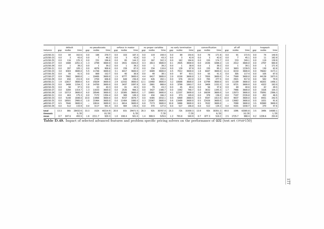
177
default no pseudocosts enforce in master no proper variables no early termination convexification all off knapsackinstance gap nodes time gap nodes time gap nodes time gap nodes time gap nodes time gap nodes time gap nodes time gap nodes time
p15150-21 0.0 84 162.6 0.0 186 278.7 0.0 103 187.3 0.0 119 159.4 0.0 89 154.6 0.0 78 171.9 0.0 91 172.5 0.0 74 140.9p15150-23 0.0 3 43.0 0.0 7 46.2 0.0 3 42.6 0.0 3 43.3 0.0 3 42.9 0.0 3 42.0 0.0 7 45.1 0.0 11 182.9p15150-25 0.0 116 125.3 0.0 231 196.6 0.0 85 144.2 0.0 167 242.3 0.0 162 184.6 0.0 155 174.7 0.0 233 249.1 0.0 119 130.9p15150-27 0.0 1688 2251.4 1.3 2799 3600.0 0.0 2931 3325.0 0.3 2613 3600.0 0.1 2925 3600.0 0.0 2436 3288.2 1.6 2512 3600.0 0.0 2707 660.8p15150-29 0.0 1 39.2 0.0 1 39.2 0.0 1 39.2 0.0 1 39.2 0.0 1 38.9 0.0 1 39.2 0.0 1 39.1 0.0 1 171.9p37150-21 0.0 207 105.1 0.0 4078 908.6 0.0 159 87.0 0.0 234 118.6 0.0 129 87.9 0.0 155 95.1 0.0 3603 1239.5 0.0 130 62.8p37150-23 3.0 8303 3600.0 5.5 11748 3600.0 3.1 8417 3600.0 2.7 8489 3600.0 4.5 7012 3600.0 1.8 8447 3600.0 11.4 8210 3600.0 0.0 76642 3173.1p37150-25 0.0 55 41.5 0.0 869 152.7 0.0 40 36.8 0.0 49 39.1 0.0 97 63.1 0.0 55 41.3 0.0 305 117.4 0.0 105 67.0p37150-27 0.9 7682 3600.0 – 10485 3600.0 1.5 6777 3600.0 4.4 6417 3600.0 2.0 6159 3600.0 1.2 7655 3600.0 7.4 7569 3600.0 0.0 44139 1673.5p37150-29 0.0 650 215.9 0.0 2704 606.8 0.0 648 236.8 0.0 626 202.1 0.0 576 242.0 0.0 785 277.5 0.0 2921 917.0 0.0 582 79.9p50150-21 1.9 12817 3600.0 6.4 15829 3600.0 2.9 12332 3600.0 12.1 13460 3600.0 3.2 10688 3600.0 2.9 12799 3600.0 8.5 11189 3600.0 0.0 40201 1456.1p50150-23 0.0 3408 1154.2 1.8 14700 3600.0 0.0 3437 1097.8 0.0 2881 988.6 0.0 3799 1663.7 0.0 3408 1152.3 1.8 9721 3600.0 0.0 4322 182.0p50150-25 0.0 56 37.5 0.0 63 40.3 0.0 81 44.5 0.0 79 43.2 0.0 45 40.4 0.0 56 37.8 0.0 69 48.6 0.0 42 49.5p50150-27 0.0 3284 1314.7 1.3 11633 3600.0 0.0 2536 988.2 0.0 3427 1386.7 0.0 1592 790.7 0.0 3632 1345.3 1.7 7966 3600.0 0.0 3326 154.3p50150-29 1.0 15713 3600.0 6.0 20546 3600.0 2.2 15385 3600.0 1.7 15801 3600.0 4.1 12337 3600.0 1.0 16039 3600.0 5.6 13573 3600.0 0.0 75091 2366.3p60150-21 0.0 463 175.3 0.0 7172 1354.4 0.0 389 149.3 0.0 434 166.2 0.0 373 165.0 0.0 378 138.2 0.0 7107 2226.8 0.0 452 46.5p60150-23 0.0 5148 1648.0 10.0 13466 3600.0 0.0 9157 3076.7 0.0 6365 2032.1 0.0 6469 2660.5 0.0 5547 1813.5 10.0 9637 3600.0 0.0 6551 242.5p60150-25 0.0 18501 2985.0 1.0 21964 3600.0 0.0 11484 1880.5 0.3 23367 3600.0 0.6 13489 3600.0 0.5 22426 3600.0 1.0 13682 3600.0 0.0 1831 91.6p60150-27 6.5 7646 3600.0 – 10614 3600.0 11.1 6814 3600.0 6.8 7173 3600.0 10.8 5986 3600.0 6.5 7632 3600.0 – 7090 3600.0 3.5 92880 3600.0p60150-29 0.0 512 133.9 0.0 3117 591.4 0.0 484 135.6 0.0 470 127.0 0.0 517 166.0 0.0 512 134.2 0.0 4101 1030.7 0.0 270 47.6
total 13.3 86k 28432.6 33.3 152k 40214.9 20.8 81k 29471.5 28.3 92k 30787.8 25.3 72k 31500.3 13.9 92k 30351.2 49.0 109k 42085.8 3.5 349k 14580.1timeouts 5/20 10/20 5/20 7/20 7/20 6/20 10/20 1/20mean 0.7 847.6 493.5 1.8 2211.7 920.3 1.0 830.4 501.0 1.4 908.9 529.6 1.2 793.8 540.9 0.7 877.3 518.2 2.5 1725.7 988.4 0.2 1228.6 253.8
Table D.49. Impact of selected advanced features and problem specific pricing solvers on the performance of GCG (test set cpmp150)

178A
ppendix
D.
Tables
default no pseudocosts enforce in master no proper variables no early termination convexification all off knapsackinstance gap nodes time gap nodes time gap nodes time gap nodes time gap nodes time gap nodes time gap nodes time gap nodes time
p20200-32 0.0 889 2482.8 4.2 973 3600.0 0.0 944 2110.2 0.0 738 1884.9 0.0 863 2241.8 0.0 789 1971.8 – 902 3600.0 0.0 1168 772.4p20200-34 0.0 508 1187.2 2.4 1800 3600.0 0.0 684 1367.3 0.0 388 1024.9 0.0 524 1427.0 0.0 492 1296.8 0.9 1505 3600.0 0.0 495 918.1p20200-36 0.0 62 293.0 0.0 173 465.6 0.0 36 274.9 0.0 52 328.0 0.0 39 279.6 0.0 33 269.1 0.0 273 756.8 0.0 48 650.7p50200-36 0.0 2488 1234.3 3.3 10835 3600.0 0.0 1927 1085.1 0.0 2943 1263.1 0.0 2014 1287.7 0.0 889 532.6 3.3 6576 3600.0 0.0 1741 282.7p50200-37 0.0 2650 1067.9 3.6 11594 3600.0 0.0 3133 1237.4 0.0 2438 999.8 0.0 2284 1126.1 0.0 5811 1950.5 2.5 7897 3600.0 0.0 4203 478.4p50200-39 0.0 1176 589.7 1.2 11374 3600.0 0.0 2301 972.2 0.0 1029 500.9 0.0 1122 669.1 0.0 1850 822.6 0.9 7386 3600.0 0.0 1324 284.0p66200-31 0.0 1148 377.0 0.0 14290 2823.5 0.0 2120 563.1 0.0 1133 345.3 0.0 677 336.1 0.0 1524 451.4 0.2 9874 3600.0 0.0 1753 230.7p66200-36 0.0 4533 1606.2 2.9 13653 3600.0 0.0 5149 1886.4 0.0 5243 1902.5 0.0 6404 3151.3 0.0 5171 1878.0 2.0 7947 3600.0 0.0 6510 500.8p66200-38 0.6 8346 3600.0 3.2 12556 3600.0 1.8 8663 3600.0 2.0 8677 3600.0 1.5 6709 3600.0 4.4 9066 3600.0 2.7 7156 3600.0 0.0 22744 1403.8p80200-33 0.8 10218 3600.0 5.4 11499 3600.0 1.4 10176 3600.0 0.9 10834 3600.0 0.8 7802 3600.0 1.3 10768 3600.0 5.4 7875 3600.0 0.0 15458 788.7p80200-34 0.9 4554 3600.0 – 6542 3600.0 1.0 4530 3600.0 2.7 4614 3600.0 0.7 3602 3600.0 0.7 4861 3600.0 – 4116 3600.0 0.0 15096 891.9p80200-38 0.0 1656 695.6 0.6 10717 3600.0 0.0 1464 652.7 0.0 1345 643.3 0.0 1246 839.1 0.0 1656 693.4 0.8 6747 3600.0 0.0 1343 181.3
total 2.3 38k 20333.7 26.8 106k 39289.1 4.2 41k 20949.3 5.6 39k 19692.7 3.0 33k 22157.8 6.4 42k 20666.2 18.7 68k 40356.8 0.0 71k 7383.5timeouts 3/12 10/12 3/12 3/12 3/12 3/12 11/12 0/12mean 0.2 1753.3 1243.9 2.4 5577.7 2978.0 0.3 1926.6 1343.6 0.5 1666.0 1192.0 0.2 1486.3 1352.7 0.5 1776.8 1265.0 1.7 4025.6 3162.8 0.0 2338.0 519.3
Table D.50. Impact of selected advanced features and problem specific pricing solvers on the performance of GCG (test set cpmp200)
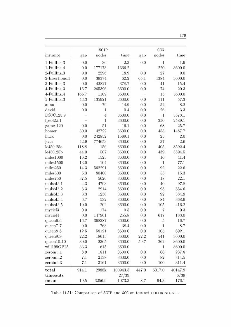
179
SCIP GCGinstance gap nodes time gap nodes time
1-FullIns 3 0.0 36 2.3 0.0 1 1.91-FullIns 4 0.0 177173 1366.2 – 220 3600.02-FullIns 3 0.0 2296 18.9 0.0 27 9.02-Insertions 3 0.0 39374 62.2 65.1 1384 3600.03-FullIns 3 0.0 42827 378.7 0.0 41 15.44-FullIns 3 16.7 265396 3600.0 0.0 74 20.34-FullIns 4 166.7 1109 3600.0 – 15 3600.05-FullIns 3 43.3 135921 3600.0 0.0 111 57.3anna 0.0 79 14.9 0.0 52 8.2david 0.0 1 0.4 0.0 26 3.3DSJC125.9 – 4 3600.0 0.0 1 3573.1fpsol2.i.1 – 1 3600.0 0.0 250 2589.1games120 0.0 51 16.1 0.0 68 25.7homer 30.0 42722 3600.0 0.0 458 1487.7huck 0.0 242852 1589.1 0.0 25 2.0jean 42.9 774653 3600.0 0.0 37 2.6le450 25a 118.8 156 3600.0 0.0 405 3592.4le450 25b 44.0 507 3600.0 0.0 439 3594.5miles1000 16.2 1525 3600.0 0.0 16 41.4miles1500 13.0 104 3600.0 0.0 1 77.1miles250 14.3 562291 3600.0 0.0 92 22.6miles500 5.3 80400 3600.0 0.0 55 15.3miles750 37.5 5626 3600.0 0.0 18 22.1mulsol.i.1 4.3 4793 3600.0 0.0 40 97.8mulsol.i.2 3.3 2914 3600.0 0.0 93 354.6mulsol.i.3 3.3 1236 3600.0 0.0 92 384.9mulsol.i.4 6.7 532 3600.0 0.0 84 368.9mulsol.i.5 10.0 202 3600.0 0.0 105 416.2myciel3 0.0 174 0.5 0.0 7 0.3myciel4 0.0 147961 255.8 0.0 617 183.0queen6 6 16.7 368387 3600.0 0.0 5 16.7queen7 7 0.0 763 38.4 0.0 1 8.7queen8 8 12.5 58121 3600.0 0.0 105 692.1queen9 9 22.2 18615 3600.0 22.2 541 3600.0queen10 10 30.0 2365 3600.0 59.7 262 3600.0will199GPIA 33.3 615 3600.0 – 1 3600.0zeroin.i.1 8.9 1811 3600.0 0.0 66 237.8zeroin.i.2 7.1 2138 3600.0 0.0 82 314.5zeroin.i.3 7.1 3161 3600.0 0.0 100 311.4
total 914.1 2988k 100943.5 447.0 6017.0 40147.9timeouts 27/39 6/39mean 19.5 3256.9 1073.3 8.7 64.3 176.1
Table D.51: Comparison of SCIP and GCG on test set coloring-all

180 Appendix D. Tables
SCIP GCGinstance gap nodes time gap nodes time
p550-1 0.0 163 8.0 0.0 32 12.2p550-2 0.0 1 1.0 0.0 1 3.8p550-3 0.0 2 1.9 0.0 3 6.6p550-4 0.0 2 1.1 0.0 1 6.2p550-5 0.0 1 1.6 0.0 1 7.3p550-6 0.0 1 1.7 0.0 1 4.0p550-7 0.0 154 8.7 0.0 15 13.4p550-8 0.0 9043 33.6 0.0 1561 599.0p550-9 0.0 10 3.6 0.0 9 6.2p550-10 0.0 3294 19.6 0.0 43 40.8p1250-1 0.0 114 2.9 0.0 173 19.3p1250-2 0.0 4 2.0 0.0 17 4.3p1250-3 0.0 1193 8.4 0.0 155 19.2p1250-4 0.0 168567 192.0 0.0 2406 275.4p1250-5 0.0 1526 10.4 0.0 68 11.9p1250-6 0.0 47464 100.5 0.0 472 57.1p1250-7 0.0 170655 328.1 0.0 1514 177.7p1250-8 0.0 20866 46.4 0.0 117 17.9p1250-9 0.0 88223 119.6 0.0 138 37.2p1250-10 0.0 219478 455.9 0.0 1175 179.9p1650-1 0.0 160 2.5 0.0 8 2.6p1650-2 0.0 4985 9.3 0.0 78 9.2p1650-3 0.0 32 2.5 0.0 13 2.9p1650-4 0.0 8313 12.8 0.0 53 8.3p1650-5 0.0 1625 5.0 0.0 59 8.7p1650-6 0.0 879 9.6 0.0 13 3.6p1650-7 0.0 2132 14.4 0.0 75 10.1p1650-8 0.0 293989 484.0 0.0 12679 1256.0p1650-9 0.0 4616 20.6 0.0 198 27.2p1650-10 0.0 64647 136.7 0.0 2367 294.9p2050-1 0.0 5157 6.8 0.0 38 4.7p2050-2 0.0 1138 3.8 0.0 86 9.9p2050-3 0.0 598 9.3 0.0 11 3.5p2050-4 0.0 57 2.8 0.0 20 3.2p2050-5 0.0 1969 14.2 0.0 5 2.9p2050-6 0.0 2 2.0 0.0 4 2.8p2050-7 0.0 15742 17.7 0.0 5 3.0p2050-8 0.0 209862 368.0 0.0 630 79.5p2050-9 0.0 47674 113.6 0.0 343 47.3p2050-10 4.8 1612769 3600.0 0.0 692 110.5
total 4.8 3007k 6182.6 0.0 25k 3390.2timeouts 1/40 0/40mean 0.1 1652.9 25.8 0.0 80.9 23.9
Table D.52: Comparison of SCIP and GCG on test set cpmp50

181
SCIP GCGinstance gap nodes time gap nodes time
p10100-11 0.0 3746 36.9 0.0 35 63.1p10100-12 0.0 2156 73.4 0.0 45 78.0p10100-13 0.0 840 40.6 0.0 7 20.1p10100-14 0.0 12118 194.0 0.0 279 261.6p10100-15 0.0 11975 164.6 0.0 235 245.6p10100-16 0.0 478 30.3 0.0 19 45.7p10100-17 0.0 3163 77.8 0.0 134 147.1p10100-18 0.0 11269 173.1 0.0 325 259.1p10100-19 0.0 2102 59.4 0.0 19 33.4p10100-20 1.4 305944 3600.0 0.8 4165 3600.0p25100-11 0.0 161357 1492.2 0.0 5202 881.0p25100-12 0.0 5428 90.9 0.0 2060 315.5p25100-13 1.3 428360 3600.0 1.4 25947 3600.0p25100-14 0.0 69642 701.5 0.0 3252 660.1p25100-15 0.0 28588 301.5 0.0 778 205.9p25100-16 2.1 345276 3600.0 0.0 11592 2180.9p25100-17 0.0 1765 64.5 0.0 47 29.2p25100-18 0.0 12876 247.6 0.0 149 72.7p25100-19 1.9 408594 3600.0 0.0 8501 1644.4p25100-20 16.1 130000 3600.0 17.2 9342 3600.0p33100-11 0.0 6679 97.7 0.0 558 86.1p33100-12 1.1 461239 3600.0 0.5 30731 3600.0p33100-13 0.0 602 33.9 0.0 185 37.6p33100-14 1.2 438288 3600.0 0.0 4447 643.6p33100-15 0.0 3056 72.4 0.0 250 56.6p33100-16 0.0 307493 2689.4 0.0 12470 2079.5p33100-17 0.0 29666 341.5 0.0 218 48.4p33100-18 0.0 68763 754.7 1.3 23614 3600.0p33100-19 0.0 43911 421.4 0.0 4076 619.2p33100-20 1.2 354820 3600.0 0.0 959 264.3p40100-11 0.0 24484 255.0 0.0 7957 1140.7p40100-12 1.3 435786 3600.0 0.0 16184 2035.2p40100-13 0.0 2038 54.8 0.0 623 83.6p40100-14 0.0 30323 352.9 0.0 329 82.0p40100-15 0.0 14780 183.4 0.0 828 156.2p40100-16 0.0 6621 121.1 0.0 283 57.6p40100-17 1.1 429574 3600.0 0.0 2218 426.8p40100-18 0.0 291995 2584.2 0.0 1732 351.4p40100-19 0.0 61675 726.2 0.0 3173 540.5p40100-20 3.7 386116 3600.0 0.0 297 90.8
total 32.4 5343k 52036.9 21.2 183k 33943.5timeouts 11/40 5/40mean 0.8 28557.8 436.9 0.5 929.5 298.0
Table D.53: Comparison of SCIP and GCG on test set cpmp100

182 Appendix D. Tables
SCIP GCGinstance gap nodes time gap nodes time
p15150-21 0.0 3313 165.4 0.0 84 163.0p15150-22 0.7 103476 3600.0 0.0 363 503.8p15150-23 0.0 1155 122.7 0.0 3 43.2p15150-24 0.0 52924 687.3 0.0 10 68.9p15150-25 0.0 12174 401.1 0.0 116 125.8p15150-26 0.0 3358 175.2 0.0 47 130.3p15150-27 0.0 63122 1993.3 0.0 1688 2278.4p15150-28 0.0 434 22.3 0.0 11 49.9p15150-29 0.0 11 12.1 0.0 1 39.5p15150-30 0.0 984 90.6 0.0 3 39.3p37150-21 0.0 17054 587.8 0.0 207 107.2p37150-22 2.0 148746 3600.0 0.0 6685 2261.6p37150-23 14.4 65070 3600.0 3.0 8220 3600.0p37150-24 0.0 89401 2242.1 0.0 2332 584.6p37150-25 0.0 2364 160.9 0.0 55 42.0p37150-26 0.0 10991 326.5 0.0 156 79.4p37150-27 12.7 57700 3600.0 0.9 7613 3600.0p37150-28 0.0 33572 767.7 0.0 7164 1600.0p37150-29 0.0 15015 392.0 0.0 650 218.4p37150-30 0.6 167437 3600.0 0.0 6819 1621.8p50150-21 1.4 156359 3600.0 1.9 12666 3600.0p50150-22 10.0 68778 3600.0 9.0 11479 3600.0p50150-23 3.9 98421 3600.0 0.0 3408 1165.9p50150-24 1.5 128420 3600.0 0.0 3487 886.8p50150-25 0.0 32871 91.5 0.0 56 38.6p50150-26 0.0 11194 379.3 0.0 4071 927.0p50150-27 1.1 129987 3600.0 0.0 3284 1325.9p50150-28 0.0 2604 138.8 0.0 435 115.4p50150-29 1.4 148682 3600.0 1.0 15627 3600.0p50150-30 2.1 151174 3600.0 0.5 16284 3600.0p60150-21 1.1 153650 3600.0 0.0 463 177.3p60150-22 6.5 84866 3600.0 0.0 5143 1816.3p60150-23 14.7 40000 3600.0 0.0 5148 1670.7p60150-24 2.6 121739 3600.0 0.4 15024 3600.0p60150-25 0.0 987 88.0 0.0 18501 3048.5p60150-26 4.4 551447 3600.0 0.0 1637 337.3p60150-27 25.7 52747 3600.0 6.5 7593 3600.0p60150-28 1.0 177083 3600.0 0.0 6364 1160.3p60150-29 0.0 874 78.1 0.0 512 135.8p60150-30 0.0 7525 231.8 0.0 1007 221.4
total 107.8 2967k 77554.5 23.2 174k 51784.3timeouts 19/40 8/40mean 2.6 22250.3 846.8 0.6 979.1 513.9
Table D.54: Comparison of SCIP and GCG on test set cpmp150

183
SCIP GCGinstance gap nodes time gap nodes time
p20200-31 0.0 20534 1554.8 0.0 181 369.4p20200-32 2.0 53487 3600.0 0.0 889 2493.0p20200-33 0.0 36409 2330.0 0.0 203 504.7p20200-34 0.5 67579 3600.0 0.0 508 1191.7p20200-35 0.0 16443 1283.1 0.0 302 563.9p20200-36 0.0 2457 313.1 0.0 62 294.0p20200-37 0.0 2843 297.9 0.0 55 256.4p20200-38 0.4 69953 3600.0 0.0 344 697.3p20200-39 0.0 1511 287.0 0.0 25 128.4p20200-40 0.0 1355 345.7 0.0 82 222.5p50200-31 2.6 60667 3600.0 2.1 8282 3600.0p50200-32 41.6 33990 3600.0 – 2737 3600.0p50200-33 6.1 33156 3600.0 12.1 6335 3600.0p50200-34 35.6 37520 3600.0 – 3305 3600.0p50200-35 4.1 41552 3600.0 7.2 7008 3600.0p50200-36 0.0 27590 1812.3 0.0 2488 1241.7p50200-37 0.0 24845 1549.2 0.0 2650 1093.8p50200-38 17.5 33824 3600.0 – 5253 3600.0p50200-39 0.0 37494 1907.9 0.0 1176 592.1p50200-40 13.5 34586 3600.0 12.6 4880 3600.0p66200-31 0.0 1548 219.4 0.0 1148 380.2p66200-32 72.3 38044 3600.0 – 3660 3600.0p66200-33 12.6 33080 3600.0 – 6788 3600.0p66200-34 21.1 33302 3600.0 7.0 5297 3600.0p66200-35 6.9 41225 3600.0 5.5 8129 3600.0p66200-36 2.6 64980 3600.0 0.0 4533 1615.8p66200-37 3.2 54983 3600.0 10.3 10271 3600.0p66200-38 2.4 62625 3600.0 0.6 8250 3600.0p66200-39 2.1 66666 3600.0 2.2 10485 3600.0p66200-40 5.4 44502 3600.0 9.4 8142 3600.0p80200-31 1.5 83648 3600.0 3.8 11408 3600.0p80200-32 56.2 26806 3600.0 3.9 3669 3600.0p80200-33 2.8 63911 3600.0 0.8 10146 3600.0p80200-34 21.6 22430 3600.0 0.9 4555 3600.0p80200-35 0.0 68676 3283.8 0.0 7078 2585.3p80200-36 3.6 52193 3600.0 1.1 8944 3600.0p80200-37 1.6 70721 3600.0 1.3 10038 3600.0p80200-38 3.9 51824 3600.0 0.0 1656 698.1p80200-39 1.7 79323 3600.0 1.1 10841 3600.0p80200-40 13.7 19330 3600.0 5.9 7104 3600.0
total 359.1 1617k 115984.2 587.8 188k 97728.3timeouts 28/40 23/40mean 8.0 28550.0 2350.7 11.4 2248.2 1728.1
Table D.55: Comparison of SCIP and GCG on test set cpmp200

184A
ppendix
D.
Tables
SCIP GCG (32) GCG (64)instance gap nodes time gap nodes time gap nodes time
new1 1 1.3 757186 3600.0 0.0 29 201.2 0.0 3 111.4new1 2 1.7 589833 3600.0 0.0 119 979.6 0.0 13 350.5new1 3 1.6 408635 3600.0 0.0 23 359.7 0.0 9 529.5new1 4 1.7 296254 3600.0 0.0 187 1888.9 0.0 7 473.3new1 5 2.0 262849 3600.0 0.0 41 828.6 0.0 11 562.3new1 6 1.4 194120 3600.0 0.0 17 468.5 0.0 39 1143.4new1 7 1.5 163145 3600.0 0.0 27 460.6 0.0 1 478.7new1 8 1.7 161800 3600.0 0.0 13 583.6 0.0 3 350.6new1 9 1.8 108307 3600.0 0.0 87 1687.5 0.0 2 453.4new1 10 2.2 84190 3600.0 0.0 35 1085.1 0.0 7 896.1new2 1 2.0 750775 3600.0 0.0 7 109.5 0.0 3 140.0new2 2 1.4 580746 3600.0 0.0 136 898.0 0.0 44 744.7new2 3 1.1 415357 3600.0 0.0 23 299.5 0.0 2 135.9new2 4 1.2 428950 3600.0 0.0 1 118.9 0.0 1 367.1new2 5 1.9 207493 3600.0 0.0 161 1622.6 0.1 154 3600.0new2 6 2.0 198288 3600.0 0.0 11 425.6 0.0 4 326.9new2 7 1.6 188555 3600.0 0.0 36 642.2 0.0 13 740.3new2 8 1.7 142970 3600.0 0.0 13 399.6 0.0 14 782.2new2 9 1.8 75900 3600.0 0.0 31 702.4 0.0 1 293.5new2 10 1.9 131284 3600.0 0.0 151 1489.0 0.0 41 1274.4new3 1 1.3 233708 3600.0 0.0 31 1205.1 0.0 1 1205.8new3 2 1.2 89037 3600.0 0.0 119 3600.0 0.0 49 3600.0new3 3 1.3 75770 3600.0 0.0 13 1227.5 0.0 7 3599.9new3 4 1.4 84830 3600.0 0.0 39 2596.2 0.0 9 1688.5new3 5 1.7 19150 3600.0 0.0 33 1937.4 0.0 9 3039.5
continue next page

185
SCIP GCG (32) GCG (64)instance gap nodes time gap nodes time gap nodes time
new3 6 2.2 8632 3600.0 0.1 55 3600.0 0.0 39 3600.0new3 7 1.8 35455 3600.0 0.0 88 3600.0 0.0 62 3600.0new3 8 1.8 30130 3600.0 0.0 53 3535.1 0.0 5 3172.4new3 9 2.4 25500 3600.0 0.1 40 3600.0 73.8 1 3600.0new3 10 2.6 864 3600.0 0.0 45 3600.0 0.2 27 3600.0new4 1 0.0 4907 16.1 0.0 1 26.1 0.0 1 15.6new4 2 0.0 187 4.8 0.0 1 17.9 0.0 1 17.1new4 3 0.0 132 6.0 0.0 1 24.6 0.0 1 28.4new4 4 0.1 1571331 3600.0 0.0 1 73.0 0.0 1 44.5new4 5 0.0 70140 342.6 0.0 13 86.4 0.0 13 106.3new4 6 0.2 792713 3600.0 0.0 1 58.8 0.0 1 66.1new4 7 0.0 670545 3406.9 0.0 1 57.0 0.0 1 54.1new4 8 0.2 535592 3600.0 0.0 4 99.3 0.0 3 59.0new4 9 0.2 546140 3600.0 0.0 3 92.6 0.0 3 93.6new4 10 0.2 507737 3600.0 0.0 3 61.0 0.0 5 154.4new5 1 0.7 640409 3600.0 0.0 23 254.4 0.0 1 130.1new5 2 1.3 317663 3600.0 0.0 11 248.6 0.0 1 230.7new5 3 0.9 318430 3600.0 0.0 3 177.1 0.0 3 282.4new5 4 1.4 247945 3600.0 0.0 75 1445.6 0.0 3 265.3new5 5 1.4 120474 3600.0 0.0 42 871.3 0.0 17 887.4new5 6 1.3 147990 3600.0 0.0 161 3570.1 0.0 129 3600.0new5 7 1.0 135050 3600.0 0.0 133 2008.2 0.0 13 730.5new5 8 1.3 114213 3600.0 0.0 15 554.7 0.0 1 564.4new5 9 1.2 78548 3600.0 0.0 124 3600.0 0.0 87 3600.0new5 10 1.7 22990 3600.0 0.0 85 2109.2 0.0 25 1799.1
continue next page
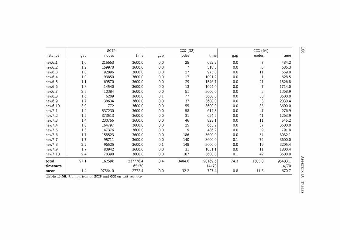
186A
ppendix
D.
Tables
SCIP GCG (32) GCG (64)instance gap nodes time gap nodes time gap nodes time
new6 1 1.0 215663 3600.0 0.0 25 692.2 0.0 7 484.2new6 2 1.2 159970 3600.0 0.0 7 518.3 0.0 3 686.3new6 3 1.0 92896 3600.0 0.0 27 975.0 0.0 11 559.0new6 4 1.0 93850 3600.0 0.0 17 1091.2 0.0 1 628.5new6 5 1.1 69570 3600.0 0.0 29 1546.7 0.0 21 1826.8new6 6 1.8 14540 3600.0 0.0 13 1094.0 0.0 7 1714.0new6 7 2.3 10384 3600.0 0.0 51 3600.0 0.0 3 1368.9new6 8 1.6 6209 3600.0 0.1 77 3600.0 0.0 38 3600.0new6 9 1.7 38634 3600.0 0.0 37 3600.0 0.0 3 2030.4new6 10 3.0 772 3600.0 0.0 55 3600.0 0.0 35 3600.0new7 1 1.4 537230 3600.0 0.0 58 614.3 0.0 7 276.9new7 2 1.5 373513 3600.0 0.0 31 624.5 0.0 41 1263.9new7 3 1.4 230756 3600.0 0.0 46 823.1 0.0 11 545.2new7 4 1.8 164797 3600.0 0.0 25 665.2 0.0 37 3600.0new7 5 1.3 147376 3600.0 0.0 9 486.2 0.0 9 791.8new7 6 1.7 158523 3600.0 0.0 186 3600.0 0.0 34 3032.1new7 7 1.7 95711 3600.0 0.0 140 3600.0 0.1 74 3600.0new7 8 2.2 96525 3600.0 0.1 148 3600.0 0.0 19 3205.4new7 9 1.7 80942 3600.0 0.0 31 1051.1 0.0 11 1800.4new7 10 2.4 78398 3600.0 0.0 107 3600.0 0.1 42 3600.0
total 97.1 16259k 237776.4 0.4 3484.0 98169.6 74.3 1305.0 95403.1timeouts 65/70 14/70 14/70mean 1.4 97564.0 2772.4 0.0 32.2 727.4 0.8 11.5 670.7
Table D.56. Comparison of SCIP and GCG on test set rap
List of Figures
2.1 Structure of the constraints in the original problem . . . . . . 102.2 Points represented by variables in convexification and discretiza-
tion approach (bounded polyhedron) . . . . . . . . . . . . . . 152.3 Points and rays represented by variables in convexification and
discretization approach (unbounded polyhedron) . . . . . . . 162.4 The polyhedra considered by the LP relaxation and the master
problem . . . . . . . . . . . . . . . . . . . . . . . . . . . . . . 23
3.1 Solving process of SCIP with detailed LP relaxation . . . . . 263.2 Solving process of GCG . . . . . . . . . . . . . . . . . . . . . . 283.3 Decomposition and setup of the SCIP instances . . . . . . . . 293.4 Illustration of the branch-and-bound tree coordination . . . . 31
4.1 The solving process of the master problem . . . . . . . . . . . 41
7.1 Illustration of the number of variables created at the root nodeand at subsequent nodes . . . . . . . . . . . . . . . . . . . . . 113
7.2 Average number of variables created per node after the rootnode . . . . . . . . . . . . . . . . . . . . . . . . . . . . . . . . 114
7.3 Average number of variables created per node after the rootnode . . . . . . . . . . . . . . . . . . . . . . . . . . . . . . . . 114
C.1 Structure of the constraint maxtrix of RAP problems . . . . . 143
187

188 List of Figures
List of Tables
4.1 Summary of the impact of different Farkas pricing strategies(convexification approach) . . . . . . . . . . . . . . . . . . . . 61
4.2 Summary of the impact of different Farkas pricing strategies(discretization approach) . . . . . . . . . . . . . . . . . . . . . 64
4.3 Summary of the impact of different reduced cost pricing strate-gies (convexification approach) . . . . . . . . . . . . . . . . . 66
4.4 Summary of the impact of different reduced cost pricing strate-gies (discretization approach) . . . . . . . . . . . . . . . . . . 69
5.1 Impact of the variable selection rule of the branching schemeon the CPMP test sets (summary) . . . . . . . . . . . . . . . 92
5.2 Impact of the decision where branching restrictions are en-forced for the CPMP test sets (summary) . . . . . . . . . . . 93
5.3 Impact of the variable selection rule and the decision wherebranching restrictions are enforced for the RAP test sets (sum-mary) . . . . . . . . . . . . . . . . . . . . . . . . . . . . . . . 94
5.4 Comparison of the convexification approach with branchingon original variables and the discretization approach with Ryanand Foster’s branching scheme for the bin packing test sets(summary) . . . . . . . . . . . . . . . . . . . . . . . . . . . . 95
5.5 Comparison of branching on original variables and Ryan andFoster’s branching scheme for the vertex coloring test set (sum-mary) . . . . . . . . . . . . . . . . . . . . . . . . . . . . . . . 96
6.1 Comparison of the root dual bound obtained by GCG and SCIP(summary) . . . . . . . . . . . . . . . . . . . . . . . . . . . . 106
7.1 Comparison of the best Farkas pricing settings for the com-plete solving process (summary) . . . . . . . . . . . . . . . . 110
7.2 Comparison of the default reduced cost pricing method withsetting “all vars” w. r. t. the branch-and-price process for theRAP test sets (summary) . . . . . . . . . . . . . . . . . . . . 112
7.3 Impact of different reduced cost pricing settings at subsequentnodes (summary) . . . . . . . . . . . . . . . . . . . . . . . . . 115
189

190 List of Tables
7.4 Performance impact of using a knapsack solver to solve thepricing problems for the CPMP test sets (summary) . . . . . 118
7.5 Summary of the impact of selected acceleration strategies forthe CPMP test sets . . . . . . . . . . . . . . . . . . . . . . . . 119
7.6 Computational results for GCG on the 180 instances of eachsize in the complete bin packing test sets (summary) . . . . . 121
7.7 Comparison of SCIP and GCG on test set coloring-all (sum-mary) . . . . . . . . . . . . . . . . . . . . . . . . . . . . . . . 121
7.8 Comparison of SCIP and GCG on the complete CPMP test sets(summary) . . . . . . . . . . . . . . . . . . . . . . . . . . . . 122
7.9 Comparison of SCIP and GCG on the complete RAP test set(summary) . . . . . . . . . . . . . . . . . . . . . . . . . . . . 123
C.1 Test sets of vertex coloring instances . . . . . . . . . . . . . . 139C.2 Test set of RAP instances . . . . . . . . . . . . . . . . . . . . 145
D.1 Computational results for Farkas pricing at the root node ontest set cpmp50s . . . . . . . . . . . . . . . . . . . . . . . . . 149
D.2 Computational results for Farkas pricing at the root node ontest set cpmp100s . . . . . . . . . . . . . . . . . . . . . . . . 149
D.3 Computational results for Farkas pricing at the root node ontest set cpmp150s . . . . . . . . . . . . . . . . . . . . . . . . 149
D.4 Computational results for Farkas pricing at the root node ontest set cpmp200s . . . . . . . . . . . . . . . . . . . . . . . . 150
D.5 Computational results for Farkas pricing at the root node ontest set coloring . . . . . . . . . . . . . . . . . . . . . . . . 150
D.6 Computational results for Farkas pricing at the root node ontest set rap32s . . . . . . . . . . . . . . . . . . . . . . . . . . 150
D.7 Computational results for Farkas pricing at the root node ontest set rap64s . . . . . . . . . . . . . . . . . . . . . . . . . . 151
D.8 Computational results for Farkas pricing at the root node ontest set bindata1-n1s . . . . . . . . . . . . . . . . . . . . . . 151
D.9 Computational results for Farkas pricing at the root node ontest set bindata1-n2s . . . . . . . . . . . . . . . . . . . . . . 151
D.10 Computational results for Farkas pricing at the root node ontest set bindata1-n3s . . . . . . . . . . . . . . . . . . . . . . 152
D.11 Computational results for reduced cost pricing at the root nodeon test set cpmp50s . . . . . . . . . . . . . . . . . . . . . . . 152
D.12 Computational results for reduced cost pricing at the root nodeon test set cpmp100s . . . . . . . . . . . . . . . . . . . . . . 152
D.13 Computational results for reduced cost pricing at the root nodeon test set cpmp150s . . . . . . . . . . . . . . . . . . . . . . 153
D.14 Computational results for reduced cost pricing at the root nodeon test set cpmp200s . . . . . . . . . . . . . . . . . . . . . . 153

List of Tables 191
D.15 Computational results for reduced cost pricing at the root nodeon test set coloring . . . . . . . . . . . . . . . . . . . . . . 153
D.16 Computational results for reduced cost pricing at the root nodeon test set rap32s . . . . . . . . . . . . . . . . . . . . . . . . 154
D.17 Computational results for reduced cost pricing at the root nodeon test set rap64s . . . . . . . . . . . . . . . . . . . . . . . . 154
D.18 Computational results for reduced cost pricing at the root nodeon test set bindata1-n1s . . . . . . . . . . . . . . . . . . . . 154
D.19 Computational results for reduced cost pricing at the root nodeon test set bindata1-n2s . . . . . . . . . . . . . . . . . . . . 155
D.20 Computational results for reduced cost pricing at the root nodeon test set bindata1-n3s . . . . . . . . . . . . . . . . . . . . 155
D.21 Computational results for the branch-and-price process on testset cpmp50s . . . . . . . . . . . . . . . . . . . . . . . . . . . 156
D.22 Computational results for the branch-and-price process on testset cpmp100s . . . . . . . . . . . . . . . . . . . . . . . . . . . 156
D.23 Computational results for the branch-and-price process on testset cpmp150s . . . . . . . . . . . . . . . . . . . . . . . . . . . 156
D.24 Computational results for the branch-and-price process on testset cpmp200s . . . . . . . . . . . . . . . . . . . . . . . . . . . 156
D.25 Computational results for the branch-and-price process on testset rap32s . . . . . . . . . . . . . . . . . . . . . . . . . . . . 157
D.26 Computational results for the branch-and-price process on testset rap64s . . . . . . . . . . . . . . . . . . . . . . . . . . . . 157
D.27 Computational results for the branch-and-price process on testset bindata1-n1s . . . . . . . . . . . . . . . . . . . . . . . . 157
D.28 Computational results for the branch-and-price process on testset bindata1-n2s . . . . . . . . . . . . . . . . . . . . . . . . 157
D.29 Computational results for the branch-and-price process on testset bindata1-n3s . . . . . . . . . . . . . . . . . . . . . . . . 158
D.30 Computational results for the branch-and-price process on testset coloring . . . . . . . . . . . . . . . . . . . . . . . . . . . 158
D.31 Comparison of the dual bound obtained by SCIP and GCG ontest set cpmp50 . . . . . . . . . . . . . . . . . . . . . . . . . . 159
D.32 Comparison of the dual bound obtained by SCIP and GCG ontest set cpmp100 . . . . . . . . . . . . . . . . . . . . . . . . . 160
D.33 Comparison of the dual bound obtained by SCIP and GCG ontest set cpmp150 . . . . . . . . . . . . . . . . . . . . . . . . . 161
D.34 Comparison of the dual bound obtained by SCIP and GCG ontest set cpmp200 . . . . . . . . . . . . . . . . . . . . . . . . . 162
D.35 Comparison of the dual bound obtained by SCIP and GCG (32constraints per block) on test set rap . . . . . . . . . . . . . 163
D.36 Comparison of the dual bound obtained by SCIP and GCG (64constraints per block) on test set rap . . . . . . . . . . . . . 164
192 List of Tables
D.37 Comparison of the dual bound obtained by SCIP and GCG ontest set coloring . . . . . . . . . . . . . . . . . . . . . . . . 165
D.38 Comparison of the dual bound obtained by SCIP and GCG ontest set bindata1-n1s . . . . . . . . . . . . . . . . . . . . . . 166
D.39 Comparison of the dual bound obtained by SCIP and GCG ontest set bindata1-n2s . . . . . . . . . . . . . . . . . . . . . . 167
D.40 Comparison of the dual bound obtained by SCIP and GCG ontest set bindata1-n3s . . . . . . . . . . . . . . . . . . . . . . 168
D.41 Impact of the reduced cost pricing setting at subsequent nodeson the performance of GCG (test set cpmp50s) . . . . . . . . . 169
D.42 Impact of the reduced cost pricing setting at subsequent nodeson the performance of GCG (test set cpmp100s) . . . . . . . . 170
D.43 Impact of the reduced cost pricing setting at subsequent nodeson the performance of GCG (test set cpmp150s) . . . . . . . . 171
D.44 Impact of the reduced cost pricing setting at subsequent nodeson the performance of GCG (test set cpmp200s) . . . . . . . . 172
D.45 Impact of the reduced cost pricing setting at subsequent nodeson the performance of GCG (test set rap32s) . . . . . . . . . 173
D.46 Impact of the reduced cost pricing setting at subsequent nodeson the performance of GCG (test set rap64s) . . . . . . . . . 174
D.47 Impact of selected advanced features and problem specific pric-ing solvers on the performance of GCG (test set cpmp50) . . . 175
D.48 Impact of selected advanced features and problem specific pric-ing solvers on the performance of GCG (test set cpmp100) . . 176
D.49 Impact of selected advanced features and problem specific pric-ing solvers on the performance of GCG (test set cpmp150) . . 177
D.50 Impact of selected advanced features and problem specific pric-ing solvers on the performance of GCG (test set cpmp200) . . 178
D.51 Comparison of SCIP and GCG on test set coloring-all . . . 179D.52 Comparison of SCIP and GCG on test set cpmp50 . . . . . . . 180D.53 Comparison of SCIP and GCG on test set cpmp100 . . . . . . 181D.54 Comparison of SCIP and GCG on test set cpmp150 . . . . . . 182D.55 Comparison of SCIP and GCG on test set cpmp200 . . . . . . 183D.56 Comparison of SCIP and GCG on test set rap . . . . . . . . . 186
Bibliography
[1] T. Achterberg. Constraint Integer Programming. PhD thesis, TechnischeUniversitat Berlin, 2007.
[2] T. Achterberg. SCIP: solving constraint integer programs. MathematicalProgramming Computation, 1(1):1–41, 2009.
[3] T. Achterberg, T. Berthold, S. Heinz, T. Koch, A. Martin, M. Pfetsch,S. Vigerske, and K. Wolter. SCIP (Solving Constraint Integer Pro-grams), documentation. http://scip.zib.de/doc.
[4] T. Achterberg, T. Berthold, T. Koch, and K. Wolter. Constraint IntegerProgramming: A new approach to integrate CP and MIP. Lecture Notesin Computer Science, 5015(2):6–20, 2008.
[5] T. Achterberg, T. Koch, and A. Martin. MIPLIB 2003. OperationsResearch Letters, 34(4):1–12, 2006. http://miplib.zib.de.
[6] T. Achterberg and C. Raack. The MCF-separator – detecting and ex-ploiting multi-commodity flows in MIPs. ZIB-Report 09-38, submittedto Mathematical Programming C, Zuse Institute Berlin, 2009.
[7] C. Alves and J. M. V. de Carvalho. A stabilized branch-and-price-and-cut algorithm for the multiple length cutting stock problem. Computers& Operations Research, 35(4):1315–1328, 2008.
[8] L. H. Applegren. A column generation algorithm for a ship schedulingproblem. Transportation Science, 3:71–78, 1969.
[9] K. R. Apt. Principles of Constraint Programming. Cambridge UniversityPress, 2003.
[10] C. Barnhart, E. L. Johnson, G. L. Nemhauser, M. W. P. Savelsbergh,and P. H. Vance. Branch-and-price: Column generation for solving hugeinteger programs. Operations Research, 46:316–329, 1996.
[11] T. Berthold. Primal Heuristics for Mixed Integer Programs. Master’sthesis, Technische Universitat Berlin, 2006.
193

194 Bibliography
[12] R. E. Bixby, M. Fenelon, Z. Gu, E. Rothberg, and R. Wunderling. Mixed-integer programming: A progress report. In M. Grotschel, editor, TheSharpest Cut: The Impact of Manfred Padberg and His Work. SIAM,2004.
[13] A. Caprara, F. Furini, and E. Malaguti. Exact algorithms for the tem-poral knapsack problem. Technical report OR-10-7, DEIS, University ofBologna, 2010.
[14] A. Ceselli. Capacitated p-median instances and corresponding format,used in [15] and [17]. http://www.dti.unimi.it/~ceselli/datasets.html.
[15] A. Ceselli. Two exact algorithms for the capacitated p-median problem.4OR, 1(4):319–340, 2003.
[16] A. Ceselli, M. Gatto, M. E. Lubbecke, M. Nunkesser, and H. Schilling.Optimizing the cargo express service of swiss federal railways. Trans-portation Science, 42(4):450–465, 2006.
[17] A. Ceselli and G. Righini. A branch and price algorithm for the capaci-tated p-median problem. Networks, 45(3):125–142, 2005.
[18] V. Chvatal. Linear programming. Freeman, 1983.
[19] E. G. Coffman, Jr., M. R. Garey, and D. S. Johnson. Approximation al-gorithms for bin-packing – an updated survey. In G. Ausiello, M. Lucer-tini, and P. Serafini, editors, Algorithm Design for Computer SystemDesign, pages 49–106. Spinger, New York, 1984.
[20] COIN-OR, 2009. http://www.coin-or.org.
[21] G. B. Dantzig, A. Orden, and P. Wolfe. The generalized simplex methodfor minimizing a linear form under linear inequality restraints. PacificJournal of Mathematics, 5(2):183–195, 1955.
[22] G. B. Dantzig and P. Wolfe. Decomposition principle for linear programs.Operations Research, 8(1):101–111, 1960.
[23] G. B. Dantzig and P. Wolfe. The decomposition algorithm for linearprograms. Econometrica, 29(4):767–778, 1961.
[24] Z. Degraeve, W. Gochet, and R. Jans. Improving discrete modelrepresentations via symmetry considerations. Management Science,47(10):1396–1407, 2001.
[25] Z. Degraeve, W. Gochet, and R. Jans. Alternative formulations for alayout problem in the fashion industry. European Journal of OperationalResearch, 143(1):80–93, 2002.

Bibliography 195
[26] G. Desaulniers, J. Desrosiers, and M. M. Solomon. Acceleration strate-gies in column generation methods for vehicle routing and crew schedul-ing problems. In C. C. Ribeiro and P. Hansen, editors, Essays abdSurveys in Metaheuristics, pages 309–324. Kluwer, Boston, 2001.
[27] G. Desaulniers, J. Desrosiers, and M. M. Solomon, editors. Column Gen-eration. GERAD 25th Anniversary Series. Springer, New York, 2005.
[28] J. Desrosiers, Y. Dumas, M. M. Solomon, and F. Soumis. Time con-strained routing and scheduling. In Handbooks in Operations Researchand Management Science: Network Routing, pages 35–139. Elsevier Sci-ence, 1995.
[29] J. Desrosiers and M. E. Lubbecke. A primer in column generation.In G. Desaulniers, J. Desrosiers, and M. M. Solomon, editors, ColumnGeneration, pages 1–32. Springer, New York, 2005.
[30] M. Fischetti, A. Lodi, and D. Salvagnin. Just MIP it! In V. Maniezzo,T. Stutzle, and S. Vos, editors, Matheuristics, pages 39–70. Springer US,2009.
[31] J. Forrest and R. Lougee-Heimer. COIN branch and cut, user guide,2005. http://www.coin-or.org/Cbc.
[32] J. J. Forrest and D. Goldfarb. Steepest edge simplex algorithms for linearprogramming. Mathematical Programming, 57(1–3):251–292, 1992.
[33] R. Fukasawa, H. Longo, J. Lysgaard, M. P. de Aragao, M. Reis,E. Uchoa, and R. F. Werneck. Robust branch-and-cut-and-price forthe capacitated vehicle routing problem. Mathematical Programming,106(3):491–511, 2006.
[34] M. R. Garey and D. S. Johnson. Computers and Intractability: a Guideto the Theory of NP-Completeness. Freeman, San Francisco, 1979.
[35] A. M. Geoffrion. Lagrangean relaxation for integer programming. Math-ematical Programming Study, 2:82–114, 1974.
[36] P. C. Gilmore and R. E. Gomory. A linear programming approach tothe cutting stock problem. Operations Research, 9(6):849–859, 1961.
[37] P. C. Gilmore and R. E. Gomory. A linear programming approach tothe cutting stock problem – part II. Operations Research, 11(6):863–888,1963.
[38] GNU. the GNU linear programming kit. http://www.gnu.org/software/glpk.
[39] M. Grotschel. Lineare Optimierung, 2004. Skriptum zur Vorlesung imWS 2003/04.
196 Bibliography
[40] M. Grotschel, L. Lovasz, and A. Schrijver. Geometric Algorithms andCombinatorial Optimization, volume 2 of Algorithms and Combinatorics.Springer, second corrected edition, 1993.
[41] O. Gunluk, L. Ladanyi, and S. de Vries. A branch-and-price algorithmand new test problems for spectrum auctions. Management Science,51(3):391–406, 2005.
[42] Gurobi Optimizer 2.0. Reference Manual, 2009. http://www.gurobi.com/html/doc/refman/.
[43] IBM ILOG CPLEX 12.10. Reference Manual, 2009. http://www-01.ibm.com/software/integration/optimization/cplex/.
[44] R. Jans. Solving lot-sizing problems on parallel identical machines usingsymmetry-breaking constraints. INFORMS J. on Computing, 21(1):123–136, 2009.
[45] M. Jepsen, B. Petersen, S. Spoorendonk, and D. Pisinger. Subset-rowinequlities applied to the vehicle routing problem with time windows.Operations Research, 56(2):497–511, 2008.
[46] D. Johnson, A. Mehrotra, and M. Trick. Color02/03/04: Graph coloringand its generalizations. http://mat.gsia.cmu.edu/COLOR04/.
[47] E. Johnson. Modelling and strong linear programs for mixed integerprogramming. In S. W. Wallace, editor, Algorithms and model formu-lations in mathematical programming, pages 1–43. Springer-Verlag NewYork, Inc., New York, NY, USA, 1989.
[48] M. Junger and S. Thienel. The ABACUS system for branch-and-cut-and-price algorithms in integer programming and combinatorial opti-mization. Softw. Pract. Exper., 30(11):1325–1352, 2000.
[49] V. Kaibel, M. Peinhardt, and M. E. Pfetsch. Orbitopal fixing. LectureNotes in Computer Science, 4513:74–88, 2007.
[50] V. Kaibel and M. E. Pfetsch. Packing and partitioning orbitopes. Math-ematical Programming, 114(1):1–36, 2008.
[51] N. Karmarkar. A new polynomial-time algorithm for linear program-ming. Combinatorica, 4(4):373–395, 1984.
[52] L. G. Khachiyan. A polynomial algorithm in linear programming. Dok-lady Akademii Nauk SSSR, 244:1093–1096, 1979.
[53] L. G. Khachiyan. A polynomial algorithm in linear programming. SovietMathematics Doklady, 20:191–194, 1979.

Bibliography 197
[54] A. Klar. Cutting planes in mixed integer programming. Master’s thesis,Technische Universitat Berlin, 2006.
[55] T. Koch. Rapid Mathematical Programming. PhD thesis, TechnischeUniversitat Berlin, 2004. ZIB-Report 04-58.
[56] N. Kohl, J. Desrosiers, O. B. G. Madsen, M. M. Solomon, and F. Soumis.2-path cuts for the vehicle routing problem with time windows. Trans-portation Science, 33(1):101–116, 1999.
[57] M. E. Lubbecke and J. Desrosiers. Selected topics in column generation.Operations Research, 53(6):1007–1023, 2005.
[58] E. Malaguti and P. Toth. A survey on vertex coloring problems. Inter-national Transactions in Operational Research, 17(1):1–34, 2010.
[59] H. Marchand, A. Martin, R. Weismantel, and L. A. Wolsey. Cuttingplanes in integer and mixed integer programming. Discrete AppliedMathematics, 123:397–446, 2002.
[60] O. Marcotte. The cutting stock problem and integer rounding. Mathe-matical Programming, 33:82–92, 1985.
[61] F. Margot. Pruning by isomorphism in branch-and-cut. MathematicalProgramming, 94(1):71–90, 2002.
[62] S. Martello and P. Toth. Knapsack Problems: Algorithms and computerImplementations. Wiley-Interscience Series in Discrete Mathematics andOptimization, New York, 1990.
[63] A. Mehrotra and M. A. Trick. A column generation approach for graphcoloring. INFORMS JOURNAL ON COMPUTING, 8(4):344–354, 1996.
[64] O. D. Merle, D. Villeneuve, J. Desrosiers, and P. Hansen. Stabilizedcolumn generation. Discrete Math, 194:229–237, 1997.
[65] R. R. Meyer. On the existence of optimal solutions to integer and mixed-integer programming problems. Mathematical Programming, 7(1):223–235, 1974.
[66] M. Minoux. A class of combinatorial optimization problems with polyno-mially solvable large scale set-covering/partitioning relaxations. RAIRO,21:105–136, 1987.
[67] H. Mittelmann. Decision tree for optimization software: Benchmarksfor optimization software, 2009. http://plato.asu.edu/bench.html.
[68] G. L. Nemhauser, M. W. P. Savelsbergh, and G. S. Sigismondi. MINTO,a Mixed INTeger Optimizer. Oper. Res. Lett., 15:47–58, 1994.
198 Bibliography
[69] G. L. Nemhauser and L. A. Wolsey. Integer and Combinatorial Opti-mization. Wiley, New York, 1988.
[70] J. Ostrowski, J. Linderoth, F. Rossi, and S. Smirglio. Orbital branching.Lecture Notes in Computer Science, 4513:104–118, 2007.
[71] J. Ostrowski, J. Linderoth, F. Rossi, and S. Smirglio. Constraint orbitalbranching. Lecture Notes in Computer Science, 5035:225–239, 2008.
[72] P. M. Pardalos, T. Mavridou, and J. Xue. The graph coloring problem:A bibiographic survey. In D.-Z. Due and P. M. Pardalos, editors, Hand-book of Combinatorial Optimization, volume 2, pages 331–395. KluwerAcademic Publishers, 1998.
[73] M. Parker and J. Ryan. A column generation algorithm for bandwidthpacking. Telecommunication Systems, 2(1):185–195, 1993.
[74] B. Petersen, D. Pisinger, and S. Spoorendonk. Chvatal-gomory rank-1cuts used in a dantzig-wolfe decomposition of the vehicle routing problemwith time windows. In The Vehicle Routing Problem: Latest Advancesand New Challenges, pages 397–420. Springer, 2008.
[75] J. Puchinger, P. J. Stuckey, M. G. Wallace, and S. Brand. Dantzig-Wolfedecomposition and branch-and-price solving in G12. Constraints, 2010.To appear.
[76] T. K. Ralphs and M. V. Galati. Decomposition in integer linear pro-gramming. In J. K. Karlof, editor, Integer Programming: Theory andPractice, pages 57–110. CRC Press, 2005.
[77] T. K. Ralphs and M. V. Galati. Decomposition and dynamic cut gen-eration in integer linear programming. Mathematical Programming,106(2):261–285, 2006.
[78] T. K. Ralphs and M. V. Galati. DIP – decomposition for integer pro-gramming. https://projects.coin-or.org/Dip, 2009.
[79] T. K. Ralphs and M. Guzelsoy. SYMPHONY version 5.2.0 user’s man-ual, 2009. http://www.coin-or.org/SYMPHONY.
[80] T. K. Ralphs and L. Ladanyi. COIN/BCP User’s Manual, 2001. http://www.coin-or.org/Presentations/bcp-man.pdf.
[81] J. Renegar. A polynomial-time algorithm, based on newton’s method,for linear programming. Mathematical Programming, 40(1–3):59–93,1988.
[82] D. M. Ryan and B. A.Foster. An integer programming approach toscheduling. In A. Wren, editor, Computer Scheduling of Public TransportUrban Passenger Vehicle and Crew Scheduling, pages 269–280. NorthHolland, Amsterdam, 1981.

Bibliography 199
[83] M. W. P. Savelsbergh. A branch and price algorithm for the generalizedassignment problem. Operations Research, 45(6):831–841, 1997.
[84] A. Scholl and R. Klein. Bin packing instances: Data set 1. http://www.wiwi.uni-jena.de/Entscheidung/binpp/.
[85] A. Schrijver. Theory of Linear and Integer Programming. John Wiley& Sons, 1986.
[86] A. Schrijver. Combinatorial optimization : polyhedra and efficiency.Springer, 2003.
[87] S. Spoorendonk. Cut and column generation. PhD thesis, TechnicalUniversity of Denmark, 2008.
[88] P. Toth and D. Vigo. The Vehicle Routing Problem. Monograph onDiscrete Mathematics and Applications. SIAM, 2002.
[89] P. H. Vance. Branch-and-price algorithms for the one-dimensional cut-ting stock problem. Computational Optimization and Applications,9(3):211–228, 1998.
[90] P. H. Vance, C. Barnhart, E. L. Johnson, and G. L. Nemhauser. Solvingbinary cutting stock problems by column generation and branch-and-bound. Computational Optimization and Applications, 3(2):111–130,1994.
[91] F. Vanderbeck. Decomposition and column generation for integer pro-grams. PhD thesis, Universite Catholique de Louvain, Louvain-la-Neuve,Belgium, 1994.
[92] F. Vanderbeck. On dantzig-wolfe decomposition in integer program-ming and ways to perform branching in a branch-and-price algorithm.Operations Research, 48(1):111–128, 2000.
[93] F. Vanderbeck. BaPCod – a generic branch-and-price code. https://wiki.bordeaux.inria.fr/realopt/pmwiki.php/Project/BaPCod,2005.
[94] F. Vanderbeck. Implementig mixed integer column generation. In G. De-saulniers, J. Desrosiers, and M. M. Solomon, editors, Column Genera-tion, pages 331–358. Springer, Berlin, 2005.
[95] F. Vanderbeck. Branching in branch-and-price: a generic scheme. Tech-nical report, Institut de Mathematiques de Bordeaux, 2009.
[96] F. Vanderbeck and M. W. P. Savelsbergh. A generic view of dantzig-wolfe decomposition in mixed integer programming. Operations ResearchLetters, 34(3):296–306, 2006.

200 Bibliography
[97] F. Vanderbeck and L. A. Wolsey. An exact algorithm for IP columngeneration. Operations Research Letters, 19(4):151–159, 1996.
[98] K. Wolter. Implementation of Cutting Plane Separators for Mixed In-teger Programs. Master’s thesis, Technische Universitat Berlin, 2006.


Die selbstandige und eigenhandige Anfertigung dieser Arbeit versichere ichan Eides statt.
Berlin, Marz 2010
Gerald Gamrath