generative adversarial networksgenerative adversarial networks a two player minimax game between a...
TRANSCRIPT
Generative Adversarial Networks
Stefano Ermon, Aditya Grover
Stanford University
Lecture 9
Stefano Ermon, Aditya Grover (AI Lab) Deep Generative Models Lecture 9 1 / 23

Recap
Model families
Autoregressive Models: pθ(x) =∏n
i=1 pθ(xi |x<i )Variational Autoencoders: pθ(x) =
∫pθ(x, z)dz
Normalizing Flow Models: pX (x; θ) = pZ(f−1θ (x)
) ∣∣∣det(∂f−1θ (x)∂x
)∣∣∣All the above families are based on maximizing likelihoods (orapproximations)
Is the likelihood a good indicator of the quality of samples generatedby the model?
Stefano Ermon, Aditya Grover (AI Lab) Deep Generative Models Lecture 9 2 / 23

Towards likelihood-free learning
Case 1: Optimal generative model will give best sample quality andhighest test log-likelihood
For imperfect models, achieving high log-likelihoods might not alwaysimply good sample quality, and vice-versa (Theis et al., 2016)
Stefano Ermon, Aditya Grover (AI Lab) Deep Generative Models Lecture 9 3 / 23

Towards likelihood-free learning
Case 2: Great test log-likelihoods, poor samples. E.g., For a discretenoise mixture model pθ(x) = 0.01pdata(x) + 0.99pnoise(x)
99% of the samples are just noiseTaking logs, we get a lower bound
log pθ(x) = log[0.01pdata(x) + 0.99pnoise(x)]
≥ log 0.01pdata(x) = log pdata(x)− log 100
For expected likelihoods, we know that
Lower bound
Epdata [log pθ(x)] ≥ Epdata [log pdata(x)]− log 100
Upper bound (via non-negativity of KL)
Epdata [log pdata(x))] ≥ Epdata [log pθ(x)]As we increase the dimension of x, absolute value of log pdata(x)increases proportionally but log 100 remains constant. Hence,Epdata
[log pθ(x)] ≈ Epdata[log pdata(x)] in very high dimensions
Stefano Ermon, Aditya Grover (AI Lab) Deep Generative Models Lecture 9 4 / 23

Towards likelihood-free learning
Case 3: Great samples, poor test log-likelihoods. E.g., Memorizingtraining set
Samples look exactly like the training set (cannot do better!)Test set will have zero probability assigned (cannot do worse!)
The above cases suggest that it might be useful to disentanglelikelihoods and samples
Likelihood-free learning consider objectives that do not dependdirectly on a likelihood function
Stefano Ermon, Aditya Grover (AI Lab) Deep Generative Models Lecture 9 5 / 23

Comparing distributions via samples
Given a finite set of samples from two distributions S1 = {x ∼ P} andS2 = {x ∼ Q}, how can we tell if these samples are from the samedistribution? (i.e., P = Q?)
Stefano Ermon, Aditya Grover (AI Lab) Deep Generative Models Lecture 9 6 / 23

Two-sample tests
Given S1 = {x ∼ P} and S2 = {x ∼ Q}, a two-sample testconsiders the following hypotheses
Null hypothesis H0: P = QAlternate hypothesis H1: P 6= Q
Test statistic T compares S1 and S2 e.g., difference in means,variances of the two sets of samples
If T is less than a threshold α, then accept H0 else reject it
Key observation: Test statistic is likelihood-free since it does notinvolve P or Q (only samples)
Stefano Ermon, Aditya Grover (AI Lab) Deep Generative Models Lecture 9 7 / 23

Generative modeling and two-sample tests
Apriori we assume direct access to S1 = D = {x ∼ pdata}In addition, we have a model distribution pθ
Assume that the model distribution permits efficient sampling (e.g.,directed models). Let S2 = {x ∼ pθ}Alternate notion of distance between distributions: Train thegenerative model to minimize a two-sample test objective between S1and S2
Stefano Ermon, Aditya Grover (AI Lab) Deep Generative Models Lecture 9 8 / 23

Two-Sample Test via a Discriminator
Finding a two-sample test objective in high dimensions is hard
In the generative model setup, we know that S1 and S2 come fromdifferent distributions pdata and pθ respectively
Key idea: Learn a statistic that maximizes a suitable notion ofdistance between the two sets of samples S1 and S2
Stefano Ermon, Aditya Grover (AI Lab) Deep Generative Models Lecture 9 9 / 23
Generative Adversarial Networks
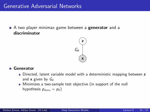
A two player minimax game between a generator and adiscriminator
x
z
Gθ
GeneratorDirected, latent variable model with a deterministic mapping between zand x given by GθMinimizes a two-sample test objective (in support of the nullhypothesis pdata = pθ)
Stefano Ermon, Aditya Grover (AI Lab) Deep Generative Models Lecture 9 10 / 23
Generative Adversarial Networks
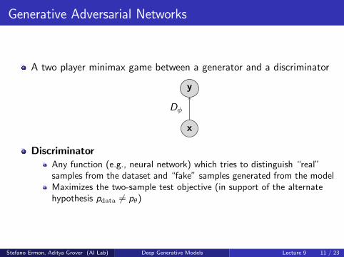
A two player minimax game between a generator and a discriminator
x
y
Dφ
DiscriminatorAny function (e.g., neural network) which tries to distinguish “real”samples from the dataset and “fake” samples generated from the modelMaximizes the two-sample test objective (in support of the alternatehypothesis pdata 6= pθ)
Stefano Ermon, Aditya Grover (AI Lab) Deep Generative Models Lecture 9 11 / 23

Example of GAN objective
Training objective for discriminator:
maxD
V (G ,D) = Ex∼pdata [logD(x)] + Ex∼pG [log(1− D(x))]
For a fixed generator G , the discriminator is performing binaryclassification with the cross entropy objective
Assign probability 1 to true data points x ∼ pdataAssing probability 0 to fake samples x ∼ pG
Optimal discriminator
D∗G (x) =
pdata(x)
pdata(x) + pG (x)
Stefano Ermon, Aditya Grover (AI Lab) Deep Generative Models Lecture 9 12 / 23

Example of GAN objective
Training objective for generator:
minG
V (G ,D) = Ex∼pdata [logD(x)] + Ex∼pG [log(1− D(x))]
For the optimal discriminator D∗G (·), we have
V (G ,D∗G (x))
= Ex∼pdata
[log pdata(x)
pdata(x)+pG (x)
]+ Ex∼pG
[log pG (x)
pdata(x)+pG (x)
]= Ex∼pdata
[log pdata(x)
pdata(x)+pG (x)
2
]+ Ex∼pG
[log pG (x)
pdata(x)+pG (x)
2
]− log 4
= DKL
[pdata,
pdata + pG2
]+ DKL
[pG ,
pdata + pG2
]︸ ︷︷ ︸
2×Jenson-Shannon Divergence (JSD)
− log 4
= 2DJSD [pdata, pG ]− log 4
Stefano Ermon, Aditya Grover (AI Lab) Deep Generative Models Lecture 9 13 / 23

Jenson-Shannon Divergence
Also called as the symmetric KL divergence
DJSD [p, q] =1
2
(DKL
[p,
p + q
2
]+ DKL
[q,
p + q
2
])Properties
DJSD [p, q] ≥ 0DJSD [p, q] = 0 iff p = qDJSD [p, q] = DJSD [q, p]√DJSD [p, q] satisfies triangle inequality → Jenson-Shannon Distance
Optimal generator for the JSD/Negative Cross Entropy GAN
pG = pdata
For the optimal discriminator D∗G∗(·) and generator G ∗(·), we have
V (G ∗,D∗G∗(x)) = − log 4
Stefano Ermon, Aditya Grover (AI Lab) Deep Generative Models Lecture 9 14 / 23

The GAN training algorithm
Sample minibatch of m training points x(1), x(2), . . . , x(m) from DSample minibatch of m noise vectors z(1), z(2), . . . , z(m) from pz
Update the generator parameters θ by stochastic gradient descent
∇θV (Gθ,Dφ) =1
m∇θ
m∑i=1
log(1− Dφ(Gθ(z(i))))
Update the discriminator parameters φ by stochastic gradient ascent
∇φV (Gθ,Dφ) =1
m∇φ
m∑i=1
[logDφ(x(i)) + log(1− Dφ(Gθ(z(i))))]
Repeat for fixed number of epochs
Stefano Ermon, Aditya Grover (AI Lab) Deep Generative Models Lecture 9 15 / 23

Alternating optimization in GANs
minθ
maxφ
V (Gθ,Dφ) = Ex∼pdata [logDφ(x)] + Ez∼p(z)[log(1− Dφ(Gθ(z)))]
Stefano Ermon, Aditya Grover (AI Lab) Deep Generative Models Lecture 9 16 / 23
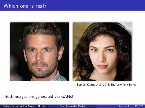
Which one is real?
Both images are generated via GANs!
Stefano Ermon, Aditya Grover (AI Lab) Deep Generative Models Lecture 9 17 / 23

Frontiers in GAN research
GANs have been successfully applied to several domains and tasks
However, working with GANs can be very challenging in practice
Unstable optimizationMode collapseEvaluation
Many bag of tricks applied to train GANs successfully
Stefano Ermon, Aditya Grover (AI Lab) Deep Generative Models Lecture 9 18 / 23

Optimization challenges
Theorem (informal): If the generator updates are made in functionspace and discriminator is optimal at every step, then the generator isguaranteed to converge to the data distribution
Unrealistic assumptions!
In practice, the generator and discriminator loss keeps oscillatingduring GAN training
No robust stopping criteria in practice (unlike likelihood basedlearning)
Stefano Ermon, Aditya Grover (AI Lab) Deep Generative Models Lecture 9 19 / 23

Mode Collapse
GANs are notorious for suffering from mode collapse
Intuitively, this refers to the phenomena where the generator of aGAN collapses to one or few samples (dubbed as “modes”)
Stefano Ermon, Aditya Grover (AI Lab) Deep Generative Models Lecture 9 20 / 23

Mode Collapse
True distribution is a mixture of Gaussians
The generator distribution keeps oscillating between different modes
Stefano Ermon, Aditya Grover (AI Lab) Deep Generative Models Lecture 9 21 / 23

Mode Collapse
Fixes to mode collapse are mostly empirically driven: alternatearchitectures, adding regularization terms, injecting small noiseperturbations etc.
https://github.com/soumith/ganhacks
How to Train a GAN? Tips and tricks to make GANs work bySoumith Chintala
Stefano Ermon, Aditya Grover (AI Lab) Deep Generative Models Lecture 9 22 / 23

Beauty lies in the eyes of the discriminator
GAN generated art auctioned at Christie’s.
Stefano Ermon, Aditya Grover (AI Lab) Deep Generative Models Lecture 9 23 / 23