generalized trichotomies: robustness and global and local ... · as condi¸c˜oes que as...
TRANSCRIPT

UNIVERSIDADE DA BEIRA INTERIOR
Ciencias
Generalized Trichotomies: robustness and global
and local invariant manifolds
Cristina Maria Gomes Tomas da Costa
Tese para obtencao do Grau de Doutor em
Matematica e Aplicacoes
(3.o ciclo de estudos)
Orientador: Prof. Doutor Antonio Jorge Gomes Bento
Covilha, fevereiro de 2018


To my parents


Acknowledgments
I would like to thank all those who, in some way, contributed to the achievement
of this thesis.
First of all I would like to specially thank my advisor, Professor Antonio Jorge
Gomes Bento, for his unconditional availability, unlimited patience and motivation
transmitted throughout the elaboration of this dissertation. Thank you for every-
thing I learned from him.
I would also like to thank my colleagues of Area Cientıfica de Matematica at
Escola Superior de Tecnologia, Instituto Politecnico de Viseu who have always sup-
ported and encouraged me until the end. A special word of thanks also to my dear
colleague and friend Manuela Ferreira.
Finally, I would like to thank my family for the care and support even in the
most difficult moments, in particular, to my husband and my sons.


Resumo
Resumo:
Num espaco de Banach, dada uma equacao diferencial v′(t) = A(t)v(t), sujeita
a uma condicao inicial v(s) = vs e que admite uma tricotomia generalizada, es-
tudamos o tipo de condicoes a impor as perturbacoes lineares B de modo que a
equacao v′(t) = [A(t) +B(t)] v(t) ainda admita uma tricotomia generalizada, ou
seja, estudamos a robustez das tricotomias generalizadas. Da mesma forma, foi
tambem objecto deste trabalho, o estudo de uma equacao diferencial com outro
tipo de perturbacoes nao lineares, v′(t) = A(t)v(t) + f(t, v). Procuramos condicoes
necessarias a impor a funcao f por forma a que a nova equacao perturbada admitisse
uma variedade invariante Lipschitz global, bem como as condicoes necessarias para
a existencia de variedades invariantes Lipschitz locais.
Palavras-Chave:
Equacoes diferenciais ordinarias nao-autonomoas, tricotomias generalizadas, robus-
tez, variedades invariantes, perturbacoes Lipschitz


Resumo Alargado
Este trabalho foi realizado no ambito do doutoramento em Matematica e Apli-
cacoes e resulta essencialmente do estudo de varios artigos na area de sistemas
dinamicos resultantes de equacoes diferenciais ordinarias. A maior inspiracao foi
obtida pela analise cuidada de artigos de Barreira e Valls [11, 5, 3], bem como de
Bento e Silva [17, 16, 20, 19], entre outros.
Sejam X um espaco de Banach, B(X) a algebra de Banach dos operadores
lineares limitados que actuam em X e A : R→ B(X) uma aplicacao contınua. Con-
sideremos a equacao diferencial ordinaria nao autonoma
v′(t) = A(t)v(t), (∗)
sujeita a uma condicao inicial v(s) = vs e suponhamos que esta equacao tem uma
solucao global. Nestas condicoes, pretendemos estudar as equacoes perturbadas
v′(t) = [A(t) +B(t)] v(t)
e
v′(t) = A(t)v(t) + f(t, v)
onde B : R→ B(X) e f : R×X → X sao funcoes contınuas. E claro que a resposta
vai depender do tipo de perturbacoes e das condicoes impostas a essas perturbacoes
e das hipoteses que assumimos sobre a equacao linear (∗).
A hipotese usada recentemente pelos autores referidos, bem como por outros,
passa por assumir que a equacao (∗) admite dicotomias ou tricotomias. Neste tra-

x Resumo Alargado
balho so consideramos tricotomias definidas de forma o mais geral possıvel. Assim,
na seccao inicial do primeiro capıtulo explicamos este conceito – tricotomias gene-
ralizadas – de uma forma muito abrangente. Considerando o operador de evolucao
Tt,s associado a equacao diferencial (∗), i.e., Tt,sv(s) = v(t) para quaisquer t, s ∈ R,
dizemos que esta admite uma decomposicao invariante se, para todo t ∈ R, existem
projeccoes Pt, Q+t , Q
−t ∈ B(X) tais que
(S1) Pt +Q+t +Q−
t = Id para todo t ∈ R;
(S2) PtQ+t = 0 para todo t ∈ R;
(S3) PtTt,s = Tt,sPs para todo t, s ∈ R;
(S4) Q+t Tt,s = Tt,sQ
+s para todo t, s ∈ R.
Definindo os subespacos lineares Et = Pt(X), F+t = Q+
t (X) e F−t = Q−
t (X) e
dadas funcoes α : R2 → R+, β+ : R2
> → R+ e β− : R2
6 → R+, onde
R26 =
(t, s) ∈ R2 : t 6 s
e R
2> =
(t, s) ∈ R2 : t > s
,
denotanto α(t, s), β+(t, s) e β−(t, s) por αt,s, β+t,s e β−
t,s, dizemos que a equacao
diferencial v′(t) = A(t)v(t) admite uma tricotomia generalizada com majorantes
α = (αt,s)(t,s)∈R2 , β+ =(β+t,s
)(t,s)∈R2
>
e β− =(β−t,s
)(t,s)∈R2
6
, ou simplesmente com
majorantes αt,s, β+t,s e β
−t,s, se admite uma decomposicao invariante tal que
(D1) ‖Tt,sPs‖ 6 αt,s para todo (t, s) ∈ R2;
(D2) ‖Tt,sQ+s ‖ 6 β+
t,s para todo (t, s) ∈ R2>;
(D3) ‖Tt,sQ−s ‖ 6 β−
t,s para todo (t, s) ∈ R26.
Ainda no primeiro capıtulo construımos, em R4, um exemplo de uma equacao
diferencial ordinaria que admite uma tricotomia generalizada que denominamos de
tricotomia−(a, b, c, d) nao uniforme, tricotomia essa que exploramos em todos os
capıtulos seguintes. Apresentamos ainda varios casos particulares deste tipo de trico-
tomias. As tricotomias ρ−exponenciais nao uniformes e exponenciais nao uniformes
sao casos particulares do anterior e vao ao encontro dos exemplos apresentados por

Resumo Alargado xi
outros autores, nomeadamente, por Barreira e Valls em [11], [12] e [2]. Alem disso,
apresentamos mais exemplos que segundo julgamos saber, sao inovadores, nomeada-
mente as tricotomias as quais demos o nome de tricotomias µ−polinomiais nao
uniformes e polinomiais nao uniformes.
No Capıtulo 2, estudamos perturbacoes lineares da equacao diferencial (∗) da
forma
v′(t) = [A(t) +B(t)]v(t),
onde B : R → B(X) e uma aplicacao contınua. Este problema designa-se usual-
mente por problema da robustez. Supondo que a equacao diferencial (∗) admite
uma tricotomia generalizada que verifica algumas hipoteses adicionais, provamos
que a equacao perturbada ira tambem admitir um comportamento tricotomico ge-
neralizado, desde que os operadores B(t) tenham norma suficientemente pequena.
Denotando B(t) por Bt e definindo as constantes, λ, λ+ e λ− a custa de αt,s, β+t,s,
β−t,s e de ‖Bt‖ da seguinte maneira:
λ := sup(t,s)∈R2
λt,sαt,s
, λ+ := sup(t,s)∈R2
>
λ+t,sβ+t,s
e λ− := sup(t,s)∈R2
6
λ−t,sβ−t,s
,
com λt,s dado por
λt,s =
∫ s
−∞
αt,r‖Br‖β−r,s dr +
∣∣∣∣∫ t
s
αt,r‖Br‖αr,s dr
∣∣∣∣+∫ +∞
t
β−t,r‖Br‖αr,s dr
+
∫ t
−∞
β+t,r‖Br‖αr,s dr +
∫ +∞
s
αt,r‖Br‖β+r,s dr,
λ+t,s definido por
λ+t,s =
∫ s
−∞
β+t,r‖Br‖αr,s dr +
∫ t
s
β+t,r‖Br‖β
+r,s dr +
∫ +∞
t
αt,r‖Br‖β+r,s dr
+
∫ s
−∞
β+t,r‖Br‖β
−r,s dr +
∫ +∞
t
β−t,r‖Br‖β
+r,s dr
e λ−t,s por
λ−t,s =
∫ t
−∞
αt,r‖Br‖β−r,s dr +
∫ s
t
β−t,r‖Br‖β
−r,s dr +
∫ +∞
s
β−t,r‖Br‖αr,s dr
+
∫ t
−∞
β+t,r‖Br‖β
−r,s dr +
∫ +∞
s
β−t,r‖Br‖β
+r,s dr,

xii Resumo Alargado
podemos enunciar o teorema que se segue.
Teorema 2.1.1 Seja X um espaco de Banach. Suponhamos que a equacao diferen-
cial v′(t) = A(t)v(t) admite uma tricotomia generalizada com majorantes αt,s, β+t,s e
β−t,s tal que
supt∈R
αt,s
αt,ℓ< +∞ para todo (ℓ, s) ∈ R2,
supt>ℓ
β+t,s
β+t,ℓ
< +∞ para todo (ℓ, s) ∈ R2>,
supt6ℓ
β−t,s
β−t,ℓ
< +∞ para todo (ℓ, s) ∈ R26.
Seja B : R→ B(X) uma funcao contınua. Se
maxλ, λ+, λ−
< 1
onde λ, λ+ and λ− estao definidos anteriormente, entao a equacao perturbada
v′(t) = [A(t) +B(t)]v(t)
admite uma tricotomia generalizada com majorantes σαt,s, σβ+t,s e σβ−
t,s e onde σ e
dado por
σ :=1
1−max λ, λ+, λ−.
Consideramos este resultado, o Teorema 2.1.1, o resultado principal deste capıtulo,
sendo enunciado no inıcio do capıtulo, mas sendo somente demonstrado na ultima
seccao deste. De seguida apresentamos casos particulares do teorema principal do
capıtulo. Comecamos por mostrar no Teorema 2.2.1 que se a tricotomia exibida
pela equacao diferencial inicial for uma tricotomia− (a, b, c, d) nao uniforme com
algumas condicoes adicionais impostas, e se a perturbacao B tambem obedecer a
certos requisitos, entao todas as condicoes do Teorema 2.1.1 sao verificadas. Os dois
exemplos seguintes, para tricotomias ρ−exponencial nao uniforme e exponencial nao
uniforme, sao apresentados como casos particulares do anterior, e e mostrado que os

Resumo Alargado xiii
resultados obtidos no caso da tricotomia exponencial sao menos exigentes do que os
obtidos por Barreira e Valls em [10]. Os dois ultimos teoremas deste capıtulo exibem
as condicoes que as tricotomias µ−polinomias nao uniformes e polinomiais nao uni-
formes devem obedecer bem como as condicoes que devemos impor as perturbacoes
por forma a serem verificadas todas as condicoes do Teorema 2.1.1. Terminamos
este capıtulo com a demonstracao do referido teorema.
No terceiro capıtulo estudamos outro tipo de problema. A equacao diferencial
inicial e sujeita agora a uma perturbacao da forma
v′(t) = A(t)v(t) + f(t, v)
onde f : R × X → X e uma funcao contınua tal que f(t, 0) = 0 e ft : X → X ,
definida por ft(x) = f(t, x), e uma funcao Lipschitz para todo o t ∈ R. Para
podermos enunciar o principal resultado deste capıtulo temos de introduzir alguma
notacao. Para cada τ ∈ R, o fluxo da equacao perturbada e definido por
Ψτ(s, vs) =(s+ τ, x(s+ τ, s, vs), y
+(s+ τ, s, vs), y−(s+ τ, s, vs)
),
com s ∈ R, vs = (ξ, η+, η−) ∈ Es × F+s × F−
s e onde
(x(t, s, vs), y
+(t, s, vs), y−(t, s, vs)
)∈ Et × F+
t × F−t
denota a solucao da equacao perturbada. Considerando o conjunto
G =⋃
t∈R
t ×Et,
e uma constante positiva N , denotamos por AN o espaco das funcoes contınuas
ϕ : G→ X tais que
ϕ(t, 0) = 0 para todo t ∈ R;
ϕ(t, ξ) ∈ F+t ⊕ F−
t para todo (t, ξ) ∈ G;
sup
∥∥ϕ(t, ξ)− ϕ(t, ξ)∥∥
∥∥ξ − ξ∥∥ : (t, ξ), (t, ξ) ∈ G, ξ 6= ξ
6 N ;

xiv Resumo Alargado
e por Vϕ o grafico de ϕ, ou seja, o conjunto
Vϕ = (s, ξ, ϕ(s, ξ)) : (s, ξ) ∈ G ⊆ R×X.
Definimos ainda as quantidades σ e ω por
σ := sup(t,s)∈R2
∣∣∣∣∫ t
s
αt,r Lip (fr)αr,s
αt,sdr
∣∣∣∣
e
ω := sups∈R
[∫ s
−∞
β+s,r Lip (fr)αr,s dr +
∫ +∞
s
β−s,r Lip (fr)αr,s dr
].
Teorema 3.1.3 Seja X um espaco de Banach. Suponhamos que v′(t) = A(t)v(t)
admite uma tricotomia generalizada com majorantes αt,s, β+t,s e β−
t,s e seja f : R ×
X → X uma funcao contınua nas condicoes descritas. Se
limr→+∞
β−s,rαr,s = lim
r→−∞β+s,rαr,s = 0 para todo s ∈ R
e
2σ + 2ω < 1,
entao existe N ∈ ]0, 1[ e uma unica funcao ϕ ∈ AN tal que
Ψτ(Vϕ) ⊂ Vϕ
para todo τ ∈ R onde Ψτ e Vϕ foram anteriormente definidos. Alem disso,
∥∥Ψt−s(s, ξ, ϕ(s, ξ))−Ψt−s(s, ξ, ϕ(s, ξ))∥∥ 6
N
ωαt,s
∥∥ξ − ξ∥∥
para todo (t, s) ∈ R2 e todo ξ, ξ ∈ Es.
O resultado global que se obteve, o Teorema 3.1.3, e feito para tricotomias gene-
ralizadas e, como tal, podemos aplica-lo a todos os exemplos de tricotomias apresen-
tados no primeiro capıtulo: tricotomias−(a, b, c, d) nao uniformes, tricotomias ρ−ex-
ponenciais nao uniformes e exponenciais nao uniformes (que sao casos particulares
do anterior) e tricotomias µ−polinomias nao uniformes e polinomiais nao uniformes.
A demonstracao deste resultado tambem e apresentada no fim do capıtulo.

Resumo Alargado xv
Terminamos este trabalho com a apresentacao, no Capıtulo 4, de um resultado
semelhante ao anterior mas em que as variedades invariantes sao locais. Aqui as
perturbacoes f : R×X → X sao funcoes contınuas tais que f(t, 0) = 0, ft(·) := f(t, ·)
e Lipschitz na bola
B(R(t)) = x ∈ X : ‖x‖ 6 R(t) ,
para todo o t ∈ R e onde R : R →]0,+∞[. Denotanto a constante de Lipschitz de
ft na bola B(R(t)) por Lip(ft|B(R(t))
), definindo σ e ω, por
σ := sup(t,s)∈R2
∣∣∣∣∣
∫ t
s
αt,r Lip(fr|B(R(r))
)αr,s
αt,s
dr
∣∣∣∣∣
e
ω := sups∈R
[∫ s
−∞
β+s,r Lip
(fr|B(R(r))
)αr,s dr +
∫ +∞
s
β−s,r Lip
(fr|B(R(r))
)αr,s dr
]
e denotanto o grafico de ϕ nas bolas B(R(t)) por
V∗ϕ,R = (s, ξ, ϕ(s, ξ)) ∈ Vϕ : ‖ξ‖ 6 R(s)
estamos em condicoes de enunciar o referido resultado.
Teorema 4.1.2 Seja X um espaco de Banach. Suponhamos que v′(t) = A(t)v(t)
admite uma tricotomia generalizada com majorantes αt,s, β+t,s e β−
t,s e seja f : R ×
X → X uma funcao contınua com as condicoes locais descritas. Se
limr→+∞
β−s,rαr,s = lim
r→−∞β+s,rαr,s = 0 para todo s ∈ R,
4σ + 4ω < 1
e
supt∈R
αt,s
R(t)< +∞ para todo s ∈ R,
entao existe N ∈ ]0, 1[ e uma funcao ϕ ∈ AN tal que para todo τ ∈ R se tem
Ψτ(V∗ϕ,R
) ⊆ V∗ϕ,R ,

xvi Resumo Alargado
onde R denota a funcao R : R→ R+ dada por
R(s) =ω
N supt∈R
[αt,s/R(t)].
Alem disso, tem-se
∥∥Ψt−s(s, ξ, ϕ(s, ξ))−Ψt−s(s, ξ, ϕ(s, ξ))∥∥ 6
N
ωαt,s
∥∥ξ − ξ∥∥
para todo (t, s) ∈ R2 e todo ξ, ξ ∈ B(R(s)) ∩ Es.
Nas duas seccoes seguintes trabalhamos com dois tipos de perturbacoes f . Uma
famılia de funcoes que verificava para todo o t ∈ R e u, v ∈ X , com q > 0
‖f(t, u)− f(t, v)‖ 6 k(t) ‖u− v‖ (‖u‖+ ‖v‖)q ,
onde k : R→ ]0,+∞[, e outra famılia que obedecia a
‖f(t, u)− f(t, v)‖ 6 k ‖u− v‖ (‖u‖+ ‖v‖)q
com k constante positiva. Para cada tipo de funcoes foram apresentados em sub-
seccoes, teoremas e corolarios para as diversas tricotomias consideradas neste tra-
balho e, em alguns casos, foi possıvel exibir o raio R, invocado no teorema local atras
apresentado, de uma forma bastante simplificada. Por fim, e feita a demonstracao
deste teorema local recorrendo ao teorema global, o Teorema 3.1.3.

Abstract
Abstract:
In a Banach space, given a differential equation v′(t) = A(t)v(t), with an ini-
tial condition v(s) = vs and that admits a generalized trichotomy, we studied
which type of conditions we need to impose to the linear perturbations B so that
v′(t) = [A(t) +B(t)] v(t) continues to admit a generalized trichotomy, that is, we
studied the robustness of generalized trichotomies. In the same way, it was also the
aim of our work the study of a differential equation with another type of nonlin-
ear perturbations, v′(t) = A(t)v(t) + f(t, v). We sought conditions to impose on
the function f so that the new perturbed equation would admit a global Lipschitz
invariant manifold as well as the necessary conditions for the existence of local Lip-
schitz invariant manifolds.
Keywords:
Nonautonomous ordinary differential equations, generalized trichotomies, robust-
ness, invariant manifolds, Lipschitz perturbations


Contents
Acknowledgements v
Resumo vii
Resumo Alargado ix
Abstract xvii
Contents xix
Introduction 1
1 Generalized Trichotomies 7
1.1 Notation and Preliminaries . . . . . . . . . . . . . . . . . . . . . . . . 7
1.2 Examples of generalized trichotomies . . . . . . . . . . . . . . . . . . 9
1.2.1 Nonuniform (a, b, c, d)−trichotomies . . . . . . . . . . . . . . . 9
1.2.2 ρ−nonuniform exponential trichotomies . . . . . . . . . . . . . 11
1.2.3 µ−nonuniform polynomial trichotomies . . . . . . . . . . . . . 13
2 Robustness 15
2.1 Main Theorem . . . . . . . . . . . . . . . . . . . . . . . . . . . . . . 16
2.2 Examples . . . . . . . . . . . . . . . . . . . . . . . . . . . . . . . . . 17
2.2.1 Nonuniform (a, b, c, d)−trichotomies . . . . . . . . . . . . . . . 17
2.2.2 ρ−nonuniform exponential trichotomies . . . . . . . . . . . . . 21
2.2.3 µ−nonuniform polynomial trichotomies . . . . . . . . . . . . . 23
2.3 Proof of Theorem 2.1.1 . . . . . . . . . . . . . . . . . . . . . . . . . . 30
2.3.1 Auxiliary Lemmas . . . . . . . . . . . . . . . . . . . . . . . . 30

xx Contents
2.3.2 Proof of Theorem 2.1.1 . . . . . . . . . . . . . . . . . . . . . . 55
3 Global Lipschitz invariant manifolds 57
3.1 Existence of global Lipschitz invariant manifolds . . . . . . . . . . . . 58
3.2 Examples of invariant center manifolds . . . . . . . . . . . . . . . . . 61
3.2.1 Nonuniform (a, b, c, d)−trichotomies . . . . . . . . . . . . . . . 61
3.2.2 ρ−nonuniform exponential trichotomies . . . . . . . . . . . . . 64
3.2.3 µ−nonuniform polynomial trichotomies . . . . . . . . . . . . . 66
3.3 Proof of Theorem 3.1.3 . . . . . . . . . . . . . . . . . . . . . . . . . . 71
3.3.1 Auxiliary Lemmas . . . . . . . . . . . . . . . . . . . . . . . . 71
3.3.2 Proof of Theorem 3.1.3 . . . . . . . . . . . . . . . . . . . . . . 81
4 Local Lipschitz invariant manifolds 83
4.1 Existence of local Lipschitz invariant manifolds . . . . . . . . . . . . 83
4.2 Examples of local invariant manifolds – first type of perturbations . . 85
4.2.1 Nonuniform (a, b, c, d)−trichotomies . . . . . . . . . . . . . . . 85
4.2.2 ρ−nonuniform exponential trichotomies . . . . . . . . . . . . . 87
4.2.3 µ−nonuniform polynomial trichotomies . . . . . . . . . . . . . 89
4.3 Examples of local invariant manifolds – second type of perturbations 94
4.3.1 Nonuniform (a, b, c, d)−trichotomies . . . . . . . . . . . . . . . 94
4.3.2 ρ−nonuniform exponential trichotomies . . . . . . . . . . . . . 96
4.3.3 µ−nonuniform polynomial trichotomies . . . . . . . . . . . . . 105
4.4 Proof of Theorem 4.1.2 . . . . . . . . . . . . . . . . . . . . . . . . . . 108
Bibliography 111
Symbols 121
Index 123

Introduction
A major problem in the study of dynamical systems is to understand which
properties are preserved when a dynamical system is perturbed. In particular, given
a Banach space X and a continuous function A, defined in R and with values in
the Banach algebra B(X) of the bounded linear operators acting on X , what are
the hypotheses that we have to assume about the solutions of the linear ordinary
differential equation
v′(t) = A(t)v(t)
and about a perturbation f : R×X → X , in order to be able to study the solutions
of the perturbed differential equation
v′(t) = A(t)v(t) + f(t, v) ?
In this context, the concept of exponential dichotomy is a very fruitful tool.
The concept of uniform exponential dichotomy goes back to 1929/30 with the
work of Perron [48, 49]. Since then, many authors have studied the role played by
uniform exponential dichotomies in dynamical systems, namely in linear ordinary
differential equations and in particularly in the study of the existence of stable and
unstable manifolds. However, the concept of uniform exponential dichotomy is very
demanding and it was convenient to consider weaker definitions.
Thus, a notion of nonuniform exponential dichotomy was used by Preda and
Megan [56] in 1983 and by Megan, Sasu and Sasu [43] in 2002 to study evolution

2 Introduction
operators. In 2006, inspired by the notion of nonuniform hyperbolic trajectories of
Pesin [50], which allowed him to obtain invariant stable manifolds for diffeomorfisms
defined on finite dimensional manifolds, Barreira and Valls [4] introduced the notion
of nonuniform exponential dichotomy for linear ordinary differential equations in
Banach spaces (see also [7]).
On the other hand, in 1994, appeared uniform dichotomies with nonexponential
growth rates presented by Pinto [51]. In the same year, Naulin and Pinto in [45] in-
troduced the concept of (h, k)−dichotomies for nonlinear differential systems. Subse-
quently, in 2010, Potzsche introduced in [55], for nonautonomous discrete equations,
nonexponential growth rates but expressed by general exponential functions.
Hence, it is natural to consider dichotomies that are simultaneous nonuniform
and nonexponential. Bento and Silva [15], in 2009, obtained stable manifolds for dif-
ference equations that admit nonuniform polynomial dichotomies where the growth
rates are more restrictive in the nonuniform part, but the uniform part obeys a
polynomial law instead of an exponential (more restrictive) law. Also in 2009 and
independently, Barreira and Valls introduced in [8] another type of nonuniform poly-
nomial dichotomy.
In 2012 and in 2013, to allow the notion of nonexponential growth and nonuni-
form behavior simultaneously and with different growth rates in the uniform and
nonuniform parts, a new nonuniform dichotomy, the nonuniform (µ, ν)−dichotomy,
was proposed by Bento and Silva in [16] for difference equations and in [18] for dif-
ferential equation. This notion includes the traditional uniform exponential dichoto-
mies, the nonuniform exponential dichotomies, the uniform polynomial dichotomies
and the nonuniform polynomial dichotomies which greatly enlarged the range of ap-
plications of uniform and nonuniform dichotomies. In these papers, Bento and Silva
also established the existence of stable local manifolds.
In 2014 and 2016, Bento and Silva considered more general growth rates for
dichotomies with nonuniform behavior for the continuous case in [20] and for the
discrete case in [21].
Introduction 3
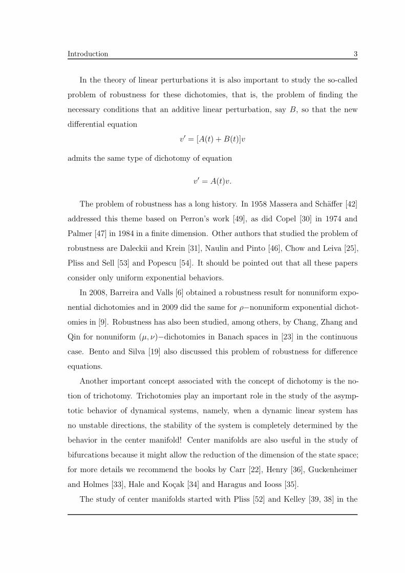
In the theory of linear perturbations it is also important to study the so-called
problem of robustness for these dichotomies, that is, the problem of finding the
necessary conditions that an additive linear perturbation, say B, so that the new
differential equation
v′ = [A(t) +B(t)]v
admits the same type of dichotomy of equation
v′ = A(t)v.
The problem of robustness has a long history. In 1958 Massera and Schaffer [42]
addressed this theme based on Perron’s work [49], as did Copel [30] in 1974 and
Palmer [47] in 1984 in a finite dimension. Other authors that studied the problem of
robustness are Daleckii and Krein [31], Naulin and Pinto [46], Chow and Leiva [25],
Pliss and Sell [53] and Popescu [54]. It should be pointed out that all these papers
consider only uniform exponential behaviors.
In 2008, Barreira and Valls [6] obtained a robustness result for nonuniform expo-
nential dichotomies and in 2009 did the same for ρ−nonuniform exponential dichot-
omies in [9]. Robustness has also been studied, among others, by Chang, Zhang and
Qin for nonuniform (µ, ν)−dichotomies in Banach spaces in [23] in the continuous
case. Bento and Silva [19] also discussed this problem of robustness for difference
equations.
Another important concept associated with the concept of dichotomy is the no-
tion of trichotomy. Trichotomies play an important role in the study of the asymp-
totic behavior of dynamical systems, namely, when a dynamic linear system has
no unstable directions, the stability of the system is completely determined by the
behavior in the center manifold! Center manifolds are also useful in the study of
bifurcations because it might allow the reduction of the dimension of the state space;
for more details we recommend the books by Carr [22], Henry [36], Guckenheimer
and Holmes [33], Hale and Kocak [34] and Haragus and Iooss [35].
The study of center manifolds started with Pliss [52] and Kelley [39, 38] in the

4 Introduction
60’s. After that, many authors studied the problem and proved results about cen-
ter manifolds. A good expository paper for the case of autonomous differential
equations in finite dimension was written by Vanderbauwhede [59] (see also Vander-
bauwhede and Gils [61]) and for the case of autonomous differential equations in
infinite dimension see Vanderbauwhede and Iooss [60]. For more details in the finite
dimensional case see Chow, Liu and Yi [27, 26] and for the infinite dimensional case
see Sijbrand [58], Mielke [44], Chow and Lu [28, 29] and Chicone and Latushkin [24].
For nonautonomous differential equations the concept of exponential trichotomy
is an important tool to obtain center manifolds theorems. This notion goes back
to Sacker and Sell [57], Aulbach [1] and Elaydi and Hajek [32] and is inspired by
the notion of exponential dichotomy that can be traced back to the work of Perron
in [48, 49]. However, as in the case of exponential dichotomies, the notion of ex-
ponential trichotomy is very demanding and several generalizations have appeared
in the literature. Essentially we can find two ways of generalization: on one hand
replace the exponential growth rates by nonexponential growth rates and on the
other hand consider exponential trichotomies that also depend on the initial time
and hence are nonuniform. Trichotomies with nonexponential growth rates have
been introduced by Fenner and Pinto in [40] where the authors study the so called
(h, k)−trichotomies and the nonuniform exponential trichotomies have been consider
by Barreira and Valls in [2, 3].
Hence, it is natural to consider trichotomies that are both nonuniform and non-
exponential. This was done by Barreira and Valls in [11, 12] where have been intro-
duced the so-called ρ−nonuniform exponential trichotomies, but these trichotomies
do not include as a particular case the (h, k)−trichotomies of Fenner and Pinto.
The robustness problem was also studied for trichotomies in 2009 by Barreira and
Valls [10] who proved the robustness of nonuniform exponential trichotomies, and
by Jiang [37] in 2012, who obtained robustness for nonuniform (µ, ν)−trichotomies.
The aim of this work is to define more general types of trichotomies in order
to study, for linear and nonlinear perturbations, the solutions of an equation of the

Introduction 5
type
v′ = A(t)v + f(t, v),
supposing that
v′ = A(t)v
admits this type of general trichotomy.
Thus, we studied the robustness of trichotomies with a general situation, included
a wide range of examples of nonuniform behavior and improved some of the existing
results.
It is also our goal the study of the differential problem
v′(t) = A(t)v + f(t, v), v(s) = vs
where nonlinear perturbations f are continuous functions with certain properties,
namely being Lipschitz functions in the second variable. Note that for dichotomies
this has already been done by Bento and Silva in [20] and in [21] for differential and
for difference equations, respectively. Here we present results both in a global and in
a local form. Initially we obtained a result on the existence of global center Lipschitz
invariant manifolds and, from this, we obtained a similar result in the existence of
local Lipschitz invariant manifolds.
Now we present the structure of this thesis. In the first chapter, we give the
basic notions and the necessary preliminaries of the generalized trichotomies for
the forward work. We also include, in a subsection, some examples of generalized
trichotomies.
In the second chapter we study the robustness problem for generalized trichot-
omies, i.e, we find necessary conditions that the linear perturbation should exhibit
in order that the trichotomy is preserved. That is the main result of the chapter.
Then we present a section with several particular cases that generalize some results
already existing in the literature. The proof of the main robustness result is given
in the last section of the chapter.

6 Introduction
In the following chapter we are going to consider another type of perturbation
of the differential equations v′ = A(t)v. Here, our main goal is to establish the
existence of global Lipschitz invariant manifolds when the linear differential equation
admits a generalized trichotomy and is submitted to a nonlinear perturbation f ,
v′(t) = A(t)v + f(t, v), satisfying some conditions. We present in the first section
the main result, in the second section particular cases of the main result and in the
last section the proof of the main result.
In the last chapter we prove, for the differential problem v′(t) = A(t)v + f(t, v),
the existence of local Lipschitz invariant manifolds. This result is stated in the first
section and proved in the last one. In the middle sections, we have considered two
types of nonlinear perturbations f and for each type of perturbation we present the
usual particular cases.

Chapter 1
Generalized Trichotomies
In this chapter we consider, on a Banach space, the notion of generalized trichot-
omy for linear ordinary differential equations which include as particular cases some
notions of tricotomies that already exist in the literature, namely in Barreira and
Valls [2, 11, 12].
§1.1 Notation and Preliminaries
Let X be a Banach space, let B(X) be the space of bounded linear operators
in X and let A : R → B(X) be a continuous map. Consider the linear differential
equation
v′ = A(t)v, v(s) = vs (1.1)
with s ∈ R, vs ∈ X . We are going to assume that (1.1) has a global solution and
denote by Tt,s the linear evolution operator associated to equation (1.1), i.e.,
v(t) = Tt,sv(s)
for every t, s ∈ R.
8 Chapter 1: Generalized Trichotomies
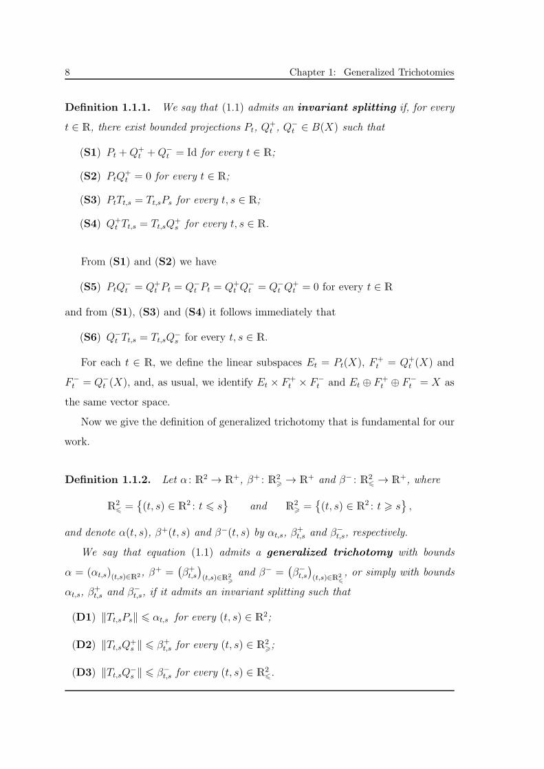
Definition 1.1.1. We say that (1.1) admits an invariant splitting if, for every
t ∈ R, there exist bounded projections Pt, Q+t , Q
−t ∈ B(X) such that
(S1) Pt +Q+t +Q−
t = Id for every t ∈ R;
(S2) PtQ+t = 0 for every t ∈ R;
(S3) PtTt,s = Tt,sPs for every t, s ∈ R;
(S4) Q+t Tt,s = Tt,sQ
+s for every t, s ∈ R.
From (S1) and (S2) we have
(S5) PtQ−t = Q+
t Pt = Q−t Pt = Q+
t Q−t = Q−
t Q+t = 0 for every t ∈ R
and from (S1), (S3) and (S4) it follows immediately that
(S6) Q−t Tt,s = Tt,sQ
−s for every t, s ∈ R.
For each t ∈ R, we define the linear subspaces Et = Pt(X), F+t = Q+
t (X) and
F−t = Q−
t (X), and, as usual, we identify Et × F+t × F−
t and Et ⊕ F+t ⊕ F−
t = X as
the same vector space.
Now we give the definition of generalized trichotomy that is fundamental for our
work.
Definition 1.1.2. Let α : R2 → R+, β+ : R2
> → R+ and β− : R2
6 → R+, where
R26 =
(t, s) ∈ R2 : t 6 s
and R
2> =
(t, s) ∈ R2 : t > s
,
and denote α(t, s), β+(t, s) and β−(t, s) by αt,s, β+t,s and β−
t,s, respectively.
We say that equation (1.1) admits a generalized trichotomy with bounds
α = (αt,s)(t,s)∈R2, β+ =
(β+t,s
)(t,s)∈R2
>
and β− =(β−t,s
)(t,s)∈R2
6
, or simply with bounds
αt,s, β+t,s and β−
t,s, if it admits an invariant splitting such that
(D1) ‖Tt,sPs‖ 6 αt,s for every (t, s) ∈ R2;
(D2) ‖Tt,sQ+s ‖ 6 β+
t,s for every (t, s) ∈ R2>;
(D3) ‖Tt,sQ−s ‖ 6 β−
t,s for every (t, s) ∈ R26.

§1.2 Examples of generalized trichotomies 9
§1.2 Examples of generalized trichotomies
§1.2.1 Nonuniform (a, b, c, d)−trichotomies
Now we present, in R4, an example of a differential equation that under certain
conditions admits a generalized trichotomy with some bounds of a special type.
This is a new and more general definition when compared to what has been done
until now and is inspired in the notions of (h, k)− dichotomy and (h, k)−trichotomy
introduced by Pinto [51], Naulin and Pinto [45] and Fenner and Pinto [40].
Example 1.2.1. Let
a, b, c, d : R→ ]0,+∞[
be C1 functions and let
εa, εb, εc, εd : R→ [1,+∞[
be C1 functions in R \ 0 and with derivatives from the left and from the right at
t = 0. In R4, equipped with the maximum norm, consider the differential equation
u′ =
[−a′(t)
a(t)+ ε∗a(t)
]u,
v′ =
[c′(t)
c(t)+ ε∗
c(t)
]v,
w′ =
[−d′(t)
d(t)+ ε∗
d(t)
]w,
z′ =
[b′(t)
b(t)+ ε∗
b(t)
]z,
(1.2)
where
ε∗i (t) =
ε′i(t)
εi(t)
cos t− 1
2− ln(εi(t))
sin t
2if t 6= 0,
0 if t = 0,
for i = a, b, c, d. Taking into account that
u′(t)
u(t)= −
a′(t)
a(t)+ ε∗
a(t)

10 Chapter 1: Generalized Trichotomies
we have
u(t) =εa(t)
(cos t−1)/2
a(t).
In a similar way we get
v(t) = c(t)εc(t)(cos t−1)/2, w(t) =
εd(t)(cos t−1)/2
d(t)and z(t) = b(t)εb(t)
(cos t−1)/2.
The evolution operator of this equation is given by
Tt,s(u, v, w, z) =(Ut,s(u, v), V
+t,sw, V
−t,sz)
where Ut,s : R2 → R
2 is defined by
Ut,s(u, v) =
(a(s)
a(t)
εa(t)(cos t−1)/2
εa(s)(cos s−1)/2u,
c(t)
c(s)
εc(t)(cos t−1)/2
εc(s)(cos s−1)/2v
)
and V +t,s, V
−t,s : R→ R are defined by
V +t,sw =
d(s)
d(t)
εd(t)(cos t−1)/2
εd(s)(cos s−1)/2w and V −
t,sz =b(t)
b(s)
εb(t)(cos t−1)/2
εb(s)(cos s−1)/2z.
Using the projections Ps, Q+s , Q
−s : R
4 → R4 given by
Ps(u, v, w, z) = (u, v, 0, 0),
Q+s (u, v, w, z) = (0, 0, w, 0),
Q−s (u, v, w, z) = (0, 0, 0, z),
we will have, for every (t, s) ∈ R2,
∥∥Tt,sQ+s
∥∥ =∥∥V +
t,s
∥∥ =d(s)
d(t)
εd(t)(cos t−1)/2
εd(s)(cos s−1)/26
d(s)
d(t)εd(s)
and∥∥Tt,sQ−
s
∥∥ =∥∥V −
t,s
∥∥ =b(t)
b(s)
εb(t)(cos t−1)/2
εb(s)(cos s−1)/26
b(t)
b(s)εb(s),
because εd(s) > 1 and εb(s) > 1. Morover, assuming that
a(s)c(s)
a(t)c(t)
(εa(t)
εc(t)
)(cos t−1)/2 (εc(s)
εa(s)
)(cos s−1)/2
> 1 for every (t, s) ∈ R2>, (1.3)

§1.2 Examples of generalized trichotomies 11
which is equivalent to
a(s)
a(t)
εa(t)((cos t−1)/2)
εa(s)(cos s−1)/2>
c(t)
c(s)
εc(t)(cos t−1)/2
εc(s)(cos s−1)/2for every (t, s) ∈ R2
>
anda(s)
a(t)
εa(t)((cos t−1)/2)
εa(s)(cos s−1)/26
c(t)
c(s)
εc(t)(cos t−1)/2
εc(s)(cos s−1)/2for every (t, s) ∈ R2
6,
we have
‖Tt,sPs‖ =
a(s)
a(t)
εa(t)(cos t−1)/2
εa(s)(cos s−1)/2for all (t, s) ∈ R2
>,
c(t)
c(s)
εc(t)(cos t−1)/2
εc(s)(cos s−1)/2for all (t, s) ∈ R2
6,
6
a(s)
a(t)εa(s) for all (t, s) ∈ R2
>,
c(t)
c(s)εc(s) for all (t, s) ∈ R2
6.
Therefore, if (1.3) is satisfied, equation (1.2) has a generalized trichotomy with
bounds
αt,s =
a(s)
a(t)εa(s)
min εa(s), εc(s)
c(t)
c(s)εc(s)
β+t,s =
d(s)
d(t)εd(s)
β−t,s =
b(t)
b(s)εb(s)
for all (t, s) ∈ R2> with t 6= s,
for all (t, s) ∈ R2 with t = s,
for all (t, s) ∈ R26 with t 6= s,
for all (t, s) ∈ R2>,
for all (t, s) ∈ R26.
(1.4)
We are going to call the trichotomies with this type of bounds by nonuniform
(a, b, c, d)−trichotomies.
§1.2.2 ρ−nonuniform exponential trichotomies
In this subsection we present particular cases of the nonuniform (a, b, c, d)−tri-
cotomies.

12 Chapter 1: Generalized Trichotomies
Example 1.2.2. Let ρ : R→ R an odd increasing differentiable function such that
limt→+∞
ρ(t) = +∞.
In (1.4), making
a(t) = e−aρ(t), c(t) = e−cρ(t), b(t) = e−bρ(t), d(t) = e−dρ(t)
and
εa(t) = εb(t) = εc(t) = εd(t) = D eε|ρ(t)|,
with
a, b, c, d,D, ε ∈ R such that D > 1 and ε > 0,
we get
αt,s =
D ea[ρ(t)−ρ(s)]+ε|ρ(s)|
D ec[ρ(s)−ρ(t)]+ε|ρ(s)|
β+t,s = D ed[ρ(t)−ρ(s)]+ε|ρ(s)|
β−t,s = D eb[ρ(s)−ρ(t)]+ε|ρ(s)|
for all (t, s) ∈ R2>,
for all (t, s) ∈ R26,
for all (t, s) ∈ R2>,
for all (t, s) ∈ R26.
(1.5)
This kind of bounds for the trichotomy, called the ρ−nonuniform exponential
trichotomy, were considered by Barreira and Valls [12, 11]. Note that in this case
condition (1.3) is equivalent to a + c > 0.
When ρ(t) = t we obtain the trichotomies considered by Barreira and Valls in [2],
the nonuniform exponential trichotomies, with the bounds of the form
αt,s =
D ea(t−s)+ε|s|
D ec(s−t)+ε|s|
β+t,s = D ed(t−s)+ε|s|
β−t,s = D eb(s−t)+ε|s|
for all (t, s) ∈ R2>,
for all (t, s) ∈ R26,
for all (t, s) ∈ R2>,
for all (t, s) ∈ R26.
Another example of ρ−nonuniform exponential trichotomies that we are going to
consider is when the function ρ is given by

§1.2 Examples of generalized trichotomies 13
ρ(t) = sgn(t) ln (1 + |t|) = ln([1 + |t|]sgn(t)
). (1.6)
It is clear that (1.6) is an odd differentiable function with
ρ′(t) =1
1 + |t|
always positive. For this choice of ρ in (1.5) we have
αt,s =
D
[(1 + |t|)sgn(t)
(1 + |s|)sgn(s)
]a(1 + |s|)ε
D
[(1 + |s|)sgn(s)
(1 + |t|)sgn(t)
]c(1 + |s|)ε
β+t,s = D
[(1 + |t|)sgn(t)
(1 + |s|)sgn(s)
]d(1 + |s|)ε
β−t,s = D
[(1 + |s|)sgn(s)
(1 + |t|)sgn(t)
]b(1 + |s|)ε
for (t, s) ∈ R2>,
for (t, s) ∈ R26,
for (t, s) ∈ R2>,
for (t, s) ∈ R26.
§1.2.3 µ−nonuniform polynomial trichotomies
Here we present another type of bounds for the trichotomy.
Example 1.2.3. Let µ : R → R be an odd, differentiable function with positive
derivative such that limt→+∞
µ(t) = +∞. Obviously µ(0) = 0. Consider a, b, c, d,D, ε
real constants with D > 1 and ε > 0. Suppose that (1.1) admits bounds such as
αt,s =
D(µ(t)− µ(s) + 1)a(|µ(s)|+ 1)ε
D(µ(s)− µ(t) + 1)c(|µ(s)|+ 1)ε
β+t,s = D(µ(t)− µ(s) + 1)d(|µ(s)|+ 1)ε
β−t,s = D(µ(s)− µ(t) + 1)b(|µ(s)|+ 1)ε
for all (t, s) ∈ R2>,
for all (t, s) ∈ R26,
for all (t, s) ∈ R2>,
for all (t, s) ∈ R26.
These trichotomies are called µ−nonuniform polynomial trichotomy.
When µ(t) = t we name the trichotomy by nonuniform polynomial trichot-
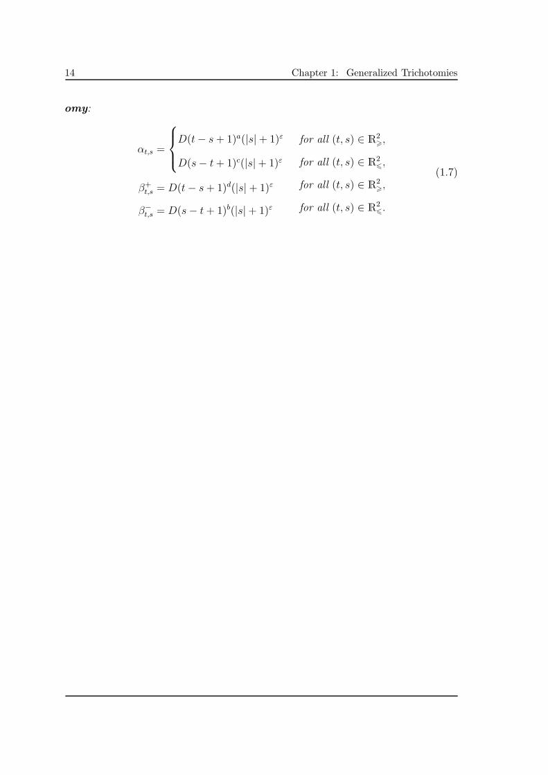
14 Chapter 1: Generalized Trichotomies
omy:
αt,s =
D(t− s+ 1)a(|s|+ 1)ε
D(s− t+ 1)c(|s|+ 1)ε
β+t,s = D(t− s+ 1)d(|s|+ 1)ε
β−t,s = D(s− t + 1)b(|s|+ 1)ε
for all (t, s) ∈ R2>,
for all (t, s) ∈ R26,
for all (t, s) ∈ R2>,
for all (t, s) ∈ R26.
(1.7)

Chapter 2
Robustness
The purpose of this chapter is the study of the robustness problem for
equation (1.1), where A : R → B(X) is a continuous map. Supposing that (1.1)
admits a generalized trichotomy with bounds αt,s, β+t,s and β−
t,s, we are going to
prove that equation
v′(t) = [A(t) +B(t)]v(t) (2.1)
also admits a generalized trichotomy when B : R→ B(X) is a continuous function
such that B(t) has sufficiently small norm.
In Section 2.1 we state the main result of this chapter, in Section 2.2 we present
several particular cases of the main theorem and in the last section we prove the
main result. Our main goal in this chapter is to unify the several settings in the
literature considering a general situation that includes a wide range of nonuniform
behaviors. Moreover, it was also our goal to improve some existing results in the
literature, namely the ones achieved by Barreira and Valls in [10].
It should be pointed out that the proof of Theorem 2.1.1 that we give in this
work is different from the proofs given by Barreira and Valls [10] for nonuniform ex-
ponential trichotomies and by Jiang [37] for nonuniform (µ, ν)−trichotomies. In [10]
and [37] the proof of robustness is made in terms of the robustness of the correspond-

16 Chapter 2: Robustness
ing dichotomies. In our work we give a direct proof without using the corresponding
robustness for the dichotomies. As far as we are aware, this proof is a new one for
trichotomies.
The results of this chapter are from Bento and Costa [14].
§2.1 Main Theorem
First we need to introduce some notation. Denoting the perturbation function
B(t) by Bt, we define the constants λ, λ+ and λ− by
λ := sup(t,s)∈R2
λt,sαt,s
, λ+ := sup(t,s)∈R2
>
λ+t,sβ+t,s
and λ− := sup(t,s)∈R2
6
λ−t,sβ−t,s
(2.2)
where λt,s is given by
λt,s =
∫ s
−∞
αt,r‖Br‖β−r,s dr +
∣∣∣∣∫ t
s
αt,r‖Br‖αr,s dr
∣∣∣∣+∫ +∞
t
β−t,r‖Br‖αr,s dr
+
∫ t
−∞
β+t,r‖Br‖αr,s dr +
∫ +∞
s
αt,r‖Br‖β+r,s dr,
(2.3)
λ+t,s is defined by
λ+t,s =
∫ s
−∞
β+t,r‖Br‖αr,s dr +
∫ t
s
β+t,r‖Br‖β
+r,s dr +
∫ +∞
t
αt,r‖Br‖β+r,s dr
+
∫ s
−∞
β+t,r‖Br‖β
−r,s dr +
∫ +∞
t
β−t,r‖Br‖β
+r,s dr
(2.4)
and λ−t,s is given by
λ−t,s =
∫ t
−∞
αt,r‖Br‖β−r,s dr +
∫ s
t
β−t,r‖Br‖β
−r,s dr +
∫ +∞
s
β−t,r‖Br‖αr,s dr
+
∫ t
−∞
β+t,r‖Br‖β
−r,s dr +
∫ +∞
s
β−t,r‖Br‖β
+r,s dr.
(2.5)
Now we state the main theorem of this chapter which says that, under certain
conditions, we can guarantee that the perturbed equation (2.1) admits a generalized
trichotomy, when (1.1) admits the same type of trichotomy.

§2.2 Examples 17
Theorem 2.1.1. Suppose that equation (1.1) admits a generalized trichotomy with
bounds αt,s, β−t,s and β+
t,s such that
supt∈R
αt,s
αt,ℓ
< +∞ for every (ℓ, s) ∈ R2, (2.6)
supt>ℓ
β+t,s
β+t,ℓ
< +∞ for every (ℓ, s) ∈ R2>, (2.7)
supt6ℓ
β−t,s
β−t,ℓ
< +∞ for every (ℓ, s) ∈ R26. (2.8)
Let B : R→ B(X) continuous. If
maxλ, λ+, λ−
< 1 (2.9)
where λ, λ+ and λ− are defined by (2.2), then equation (2.1) admits a generalized
trichotomy with bounds σαt,s, σβ+t,s and σβ−
t,s with σ given by
σ :=1
1−max λ, λ+, λ−.
The proof of this theorem will be given in the last section of the chapter.
§2.2 Examples
In this section we apply Theorem 2.1.1 to nonuniform (a, b, c, d)−trichotomies,
ρ−nonuniform exponential trichotomies and µ−nonuniform polynomial trichoto-
mies.
§2.2.1 Nonuniform (a, b, c, d)−trichotomies
We begin with the nonuniform (a, b, c, d)−trichotomies.
Theorem 2.2.1. Suppose that equation (1.1) admits a nonuniform (a, b, c, d)−tri-
chotomy. Let B : R→ B(X) be a perturbation function such that
‖Bt‖ 6 δγ(t)
max εa(t), εb(t), εc(t), εd(t)
18 Chapter 2: Robustness
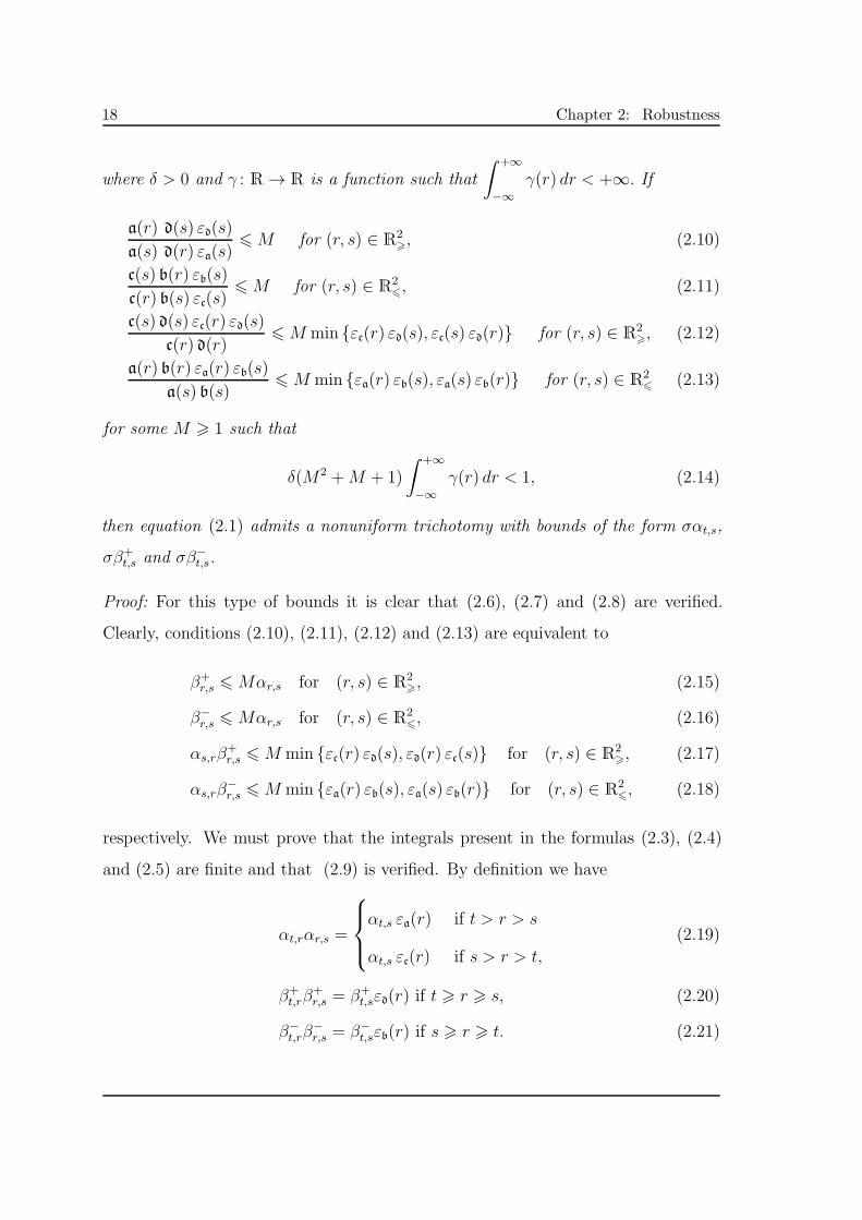
where δ > 0 and γ : R→ R is a function such that
∫ +∞
−∞
γ(r) dr < +∞. If
a(r) d(s) εd(s)
a(s) d(r) εa(s)6M for (r, s) ∈ R2
>, (2.10)
c(s) b(r) εb(s)
c(r) b(s) εc(s)6M for (r, s) ∈ R2
6, (2.11)
c(s) d(s) εc(r) εd(s)
c(r) d(r)6M min εc(r) εd(s), εc(s) εd(r) for (r, s) ∈ R2
>, (2.12)
a(r) b(r) εa(r) εb(s)
a(s) b(s)6M min εa(r) εb(s), εa(s) εb(r) for (r, s) ∈ R2
6 (2.13)
for some M > 1 such that
δ(M2 +M + 1)
∫ +∞
−∞
γ(r) dr < 1, (2.14)
then equation (2.1) admits a nonuniform trichotomy with bounds of the form σαt,s,
σβ+t,s and σβ−
t,s.
Proof: For this type of bounds it is clear that (2.6), (2.7) and (2.8) are verified.
Clearly, conditions (2.10), (2.11), (2.12) and (2.13) are equivalent to
β+r,s 6 Mαr,s for (r, s) ∈ R2
>, (2.15)
β−r,s 6 Mαr,s for (r, s) ∈ R2
6, (2.16)
αs,rβ+r,s 6M min εc(r) εd(s), εd(r) εc(s) for (r, s) ∈ R2
>, (2.17)
αs,rβ−r,s 6M min εa(r) εb(s), εa(s) εb(r) for (r, s) ∈ R2
6, (2.18)
respectively. We must prove that the integrals present in the formulas (2.3), (2.4)
and (2.5) are finite and that (2.9) is verified. By definition we have
αt,rαr,s =
αt,s εa(r) if t > r > s
αt,s εc(r) if s > r > t,
(2.19)
β+t,rβ
+r,s = β+
t,sεd(r) if t > r > s, (2.20)
β−t,rβ
−r,s = β−
t,sεb(r) if s > r > t. (2.21)

§2.2 Examples 19
Therefore, using (2.15), (2.17), (2.18), (2.16) and the last three equalities we have
αt,rβ+r,s 6
αt,sαs,rβ+r,s/εc(s) if r > s > t
Mαt,rαr,s if t > r > s
αt,rβ+r,tβ
+t,s/εd(t) if r > t > s
6
Mαt,sεd(r) if r > s > t
Mαt,sεa(r) if t > r > s
Mβ+t,sεc(r) if r > t > s
(2.22)
αt,rβ−r,s 6
αt,sαs,rβ−r,s/εa(s) if t > s > r
Mαt,rαr,s if s > r > t
αt,rβ−r,tβ
−t,s/εb(t) if s > t > r
6
Mαt,sεb(r) if t > s > r
Mαt,sεc(r) if s > r > t
Mβ−t,sεa(r) if s > t > r
(2.23)
β+t,rαr,s 6
β+t,rαr,tαt,s/εc(t) if s > t > r
Mαt,rαr,s if t > r > s
β+t,sβ
+s,rαr,s/εd(s) if t > s > r
6
Mαt,sεd(r) if s > t > r
Mαt,sεa(r) if t > r > s
Mβ+t,sεc(r) if t > s > r
(2.24)
β−t,rαr,s 6
β−t,sβ
−s,rαr,s/εb(s) if r > s > t
β−t,rαr,tαt,s/εa(t) if r > t > s
Mαt,rαr,s if s > r > t
6
Mβ−t,sεa(r) if r > s > t
Mαt,sεb(r) if r > t > s
Mαt,sεc(r) if s > r > t
(2.25)
β+t,rβ
−r,s =
β+t,sβ
+s,rβ
−r,s
εd(s)if t > s > r
β+t,rβ
−r,tβ
−t,s
εb(t)if s > t > r
6
Mβ+t,sβ
+s,rαr,s
εd(s)if t > s > r
Mαt,rβ
−r,tβ
−t,s
εb(t)if s > t > r
6
M2β+
t,sεc(r) if t > s > r
M2β−t,sεa(r) if s > t > r
(2.26)

20 Chapter 2: Robustness
and finally
β−t,rβ
+r,s =
β−t,sβ
−s,rβ
+r,s/εb(s) if r > s > t
β−t,rβ
+r,tβ
+t,s/εd(t) if r > t > s
6
Mβ−
t,sβ−s,rαr,s/εb(s) if r > s > t
Mαt,rβ+r,tβ
+t,s/εd(t) if r > t > s
6
M2β−
t,sεa(r) if r > s > t
M2β+t,sεc(r) if r > t > s.
(2.27)
We are now in conditions of prove that λ, λ+ and λ− are finite. So for every
(t, s) ∈ R2> using (2.3) and inequalities (2.19), (2.22), (2.23), (2.24) and (2.25) we
have
λt,s =
∫ s
−∞
αt,r‖Br‖β−r,s dr +
∫ t
s
αt,r‖Br‖αr,s dr +
∫ +∞
t
β−t,r‖Br‖αr,s dr+
+
∫ t
−∞
β+t,r‖Br‖αr,s dr +
∫ +∞
s
αt,r‖Br‖β+r,s dr
6(M2 +M + 1
)αt,s
∫ +∞
−∞
max εa(r), εb(r), εc(r), εd(r) ‖Br‖ dr
6 δ(M2 +M + 1
)αt,s
∫ +∞
−∞
γ(r) dr.
On the other hand, for every (t, s) ∈ R26
λt,s 6(M2 +M + 1
)αt,s
∫ +∞
−∞
max εa(r), εb(r), εc(r), εd(r) ‖Br‖ dr
6 δ(M2 +M + 1
)αt,s
∫ +∞
−∞
γ(r) dr
and therefore
λ = sup(t,s)∈R2
λt,sαt,s
6 δ(M2 +M + 1)
∫ +∞
−∞
γ(r) dr < 1
which implies that λ < +∞.
In a similar way we can prove that λ+ is finite. By (2.4) and the inequalities

§2.2 Examples 21
above (2.24), (2.20), (2.22), (2.26) and (2.27) we have for every (t, s) ∈ R2>
λ+t,s =
∫ s
−∞
β+t,r‖Br‖αr,s dr +
∫ t
s
β+t,r‖Br‖β
+r,s dr +
∫ +∞
t
αt,r‖Br‖β+r,s dr+
+
∫ s
−∞
β+t,r‖Br‖β
−r,s dr +
∫ +∞
t
β−t,r‖Br‖β
+r,s dr
6
∫ s
−∞
Mβ+t,sεc(r)‖Br‖ dr +
∫ t
s
β+t,sεd(r)‖Br‖ dr +
∫ +∞
t
Mβ+t,sεc(r)‖Br‖ dr+
+
∫ s
−∞
M2β+t,sεc(r)‖Br‖ dr +
∫ +∞
t
M2β+t,sεc(r)‖Br‖ dr
6 δ(M2 +M
)β+t,s
∫ +∞
−∞
γ(r) dr.
Finally, using (2.5) and the inequalities (2.23), (2.21), (2.25), (2.26) and (2.27)
we get, for every (t, s) ∈ R26
λ−t,s =
∫ t
−∞
αt,r‖Br‖β−r,s dr +
∫ s
t
β−t,r‖Br‖β
−r,s dr +
∫ +∞
s
β−t,r‖Br‖αr,s dr
+
∫ t
−∞
β+t,r‖Br‖β
−r,s dr +
∫ +∞
s
β−t,r‖Br‖β
+r,s dr
6
∫ t
−∞
Mβ−t,sεa(r)‖Br‖ dr +
∫ s
t
β−t,sεb(r)‖Br‖ dr +
∫ +∞
s
Mβ−t,sεa(r)‖Br‖ dr
+
∫ t
−∞
M2β−t,sεa(r)‖Br‖ dr +
∫ +∞
s
M2β−t,sεa(r)‖Br‖ dr
6 δ(M2 +M
)β−t,s
∫ +∞
−∞
γ(r) dr,
which implies that λ− < +∞.
Hence, for
δ <1
(M2 +M + 1)
∫ +∞
−∞
γ(r) dr
the condition (2.9), max λ, λ+, λ− < 1, is verified and so all the conditions required
by the theorem are satisfied. This completes the proof.
§2.2.2 ρ−nonuniform exponential trichotomies
Now, we are going to apply the last result to ρ−nonuniform exponential trichot-
omies.

22 Chapter 2: Robustness
Theorem 2.2.2. Suppose that (1.1) admits a ρ−nonuniform exponential trichot-
omy. Let B : R→ B(X) be a continuous perturbation function such that
‖Bt‖ 6δρ′(t) e−γ|ρ(t)|
D eε|ρ(t)|=
δ
Dρ′(t) e−(γ+ε)|ρ(t)|
for some δ, γ > 0 such that δ <γ
6. If
b 6 c, d 6 a, c+ d 6 0, a + b 6 0 and ε− γ < 0,
then equation (2.1) admits a ρ−nonuniform exponential trichotomy with bounds of
the form σαt,s, σβ+t,s and σβ−
t,s.
Proof: The bounds of the form (1.5) are a particular case of the bounds of the
previous example if we consider
a(t) = e−aρ(t), c(t) = e−cρ(t), b(t) = e−bρ(t), d(t) = e−dρ(t)
and
εa(t) = εb(t) = εc(t) = εd(t) = D eε|ρ(t)|,
where D > 1, ε > 0 and a, b, c, d ∈ R. Then the conditions required (2.16), (2.15),
(2.17) and (2.18) become, respectively,
b 6 c, d 6 a, c+ d 6 0 and a+ b 6 0,
with M = 1. Moreover, since γ(t) = ρ′(t) e−γ|ρ(t)| and γ > ε then∫ +∞
−∞
γ(r) dr =2
γ< +∞
and so (2.14) becomes δ <γ
6.
Corollary 2.2.3. Suppose that (1.1) admits a nonuniform exponential trichotomy
and B : R→ B(X) a continuous perturbation function such that
‖Bt‖ 6δ
De−(ε+γ)|t|,
with γ ∈ R and for some 0 < δ <γ
6. It is obvious that then equation (2.1) admits a
nonuniform exponential trichotomy with bounds of the form σαt,s, σβ+t,s and σβ−
t,s if
b 6 c, d 6 a, c+ d 6 0, a+ b 6 0 and ε− γ < 0.

§2.2 Examples 23
Here we accomplished a better result than Barreira and Valls had previously
achieved in [10]. Note that in [10] is used, in our notation, the condition
ε < min
−d − c
2,−b− a
2
which is more restricted than our hypotheses.
§2.2.3 µ−nonuniform polynomial trichotomies
Now we will consider µ−nonuniform polynomial trichotomies.
Theorem 2.2.4. Suppose that equation (1.1) admits a µ−nonuniform polynomial
trichotomy. Let B : R→ B(X) be a continuous perturbation function such that
‖Bt‖ 6 δµ′(t)(|µ(t)|+ 1)−γ,
for some γ ∈ R. If 0 < δ <|ε− γ + 1|
6D,
b 6 c 6 0, d 6 a 6 0 and ε− γ + 1 < 0,
then equation (2.1) admits a µ−nonuniform polynomial trichotomy with bounds of
the form σαt,s, σβ+t,s and σβ−
t,s.
Proof: To prove that the conditions of Theorem 2.1.1 are verified we need to compute
the integrals in formulas (2.3), (2.4) and (2.5).
It follows,
for every t 6 r 6 s,
αt,rαr,s 6 Dαt,s(|µ(r)|+ 1)ε because c 6 0,
αt,rβ−r,s 6 Dαt,s(|µ(r)|+ 1)ε because b 6 c 6 0,
β−t,rαr,s 6 αt,rαr,s 6 Dαt,s(|µ(r)|+ 1)ε because b 6 c 6 0,
for every r 6 t 6 s,
αt,rβ−r,s 6 Dαt,s(|µ(r)|+ 1)ε because b 6 c 6 0 and a 6 0,
β+t,rαr,s 6 β+
t,rαt,s 6 Dαt,s(|µ(r)|+ 1)ε because c 6 0 and d 6 0,

24 Chapter 2: Robustness
for every t 6 s 6 r,
αt,rβ+r,s 6 Dαt,s(|µ(r)|+ 1)ε because c 6 0 and d 6 0,
β−t,rαr,s 6 Dβ−
t,r(|µ(s)|+ 1)ε 6 Dαt,s(|µ(r)|+ 1)ε because a 6 0 and b 6 c 6 0.
We can also write,
for every r 6 s 6 t,
β+t,rαr,s 6 αt,rαr,s 6 Dαt,s(|µ(r)|+ 1)ε because c 6 0 and d 6 a,
αt,rβ−r,s 6 Dαt,s(|µ(r)|+ 1)ε because a 6 0 and b 6 0,
for every s 6 r 6 t,
αt,rαr,s 6 Dαt,s(|µ(r)|+ 1)ε because a 6 0,
β+t,rαr,s 6 αt,rαr,s 6 Dαt,s(|µ(r)|+ 1)ε because d 6 a 6 0,
αt,rβ+r,s 6 αt,rαr,s 6 Dαt,s(|µ(r)|+ 1)ε because d 6 a 6 0,
and for every s 6 t 6 r,
αt,rβ+r,s 6 αt,rαt,s 6 Dαt,s(|µ(r)|+ 1)ε because d 6 a and c 6 0,
β−t,rαr,s 6 β−
t,rαt,s 6 Dαt,s(|µ(r)|+ 1)ε because a 6 0 and b 6 0.
Therefore, the integrals we need to compute λt,s become,
for every (t, s) ∈ R26, if b 6 c 6 0, a 6 0 and d 6 0
∫ t
−∞
αt,r‖Br‖β−r,s dr 6 Dδαt,s
∫ t
−∞
µ′(r)(|µ(r)|+ 1)ε−γ dr, (2.28)
∫ s
t
αt,r‖Br‖β−r,s dr 6 Dδαt,s
∫ s
t
µ′(r)(|µ(r)|+ 1)ε−γ dr, (2.29)
∫ s
t
αt,r‖Br‖αr,s dr 6 Dδαt,s
∫ s
t
µ′(r)(|µ(r)|+ 1)ε−γ dr, (2.30)
∫ s
t
β−t,r‖Br‖αr,s dr 6 Dδαt,s
∫ s
t
µ′(r)(|µ(r)|+ 1)ε−γ dr, (2.31)
∫ +∞
s
β−t,r‖Br‖αr,s dr 6 Dδαt,s
∫ +∞
s
µ′(r)(|µ(r)|+ 1)ε−γ dr, (2.32)
∫ t
−∞
β+t,r‖Br‖αr,s dr 6 Dδαt,s
∫ t
−∞
µ′(r)(|µ(r)|+ 1)ε−γ dr, (2.33)
∫ +∞
s
αt,r‖Br‖β+r,s dr 6 Dδαt,s
∫ +∞
s
µ′(r)(|µ(r)|+ 1)ε−γ dr. (2.34)

§2.2 Examples 25
At last, for every (t, s) ∈ R2>, if we consider d 6 a 6 0, b 6 0 and c 6 0 then
∫ s
−∞
αt,r‖Br‖β−r,s dr 6 Dδαt,s
∫ s
−∞
µ′(r)(|µ(r)|+ 1)ε−γ dr, (2.35)
∫ t
s
αt,r‖Br‖αr,s dr 6 Dδαt,s
∫ t
s
µ′(r)(|µ(r)|+ 1)ε−γ dr, (2.36)
∫ +∞
t
β−t,r‖Br‖αr,s dr 6 Dδαt,s
∫ +∞
t
µ′(r)(|µ(r)|+ 1)ε−γ dr, (2.37)
∫ s
−∞
β+t,r‖Br‖αr,s dr 6 Dδαt,s
∫ s
−∞
µ′(r)(|µ(r)|+ 1)ε−γ dr, (2.38)
∫ t
s
β+t,r‖Br‖αr,s dr 6 Dδαt,s
∫ t
s
µ′(r)(|µ(r)|+ 1)ε−γ dr, (2.39)
∫ t
s
αt,r‖Br‖β+r,s dr 6 Dδαt,s
∫ t
s
µ′(r)(|µ(r)|+ 1)ε−γ dr (2.40)
∫ +∞
t
αt,r‖Br‖β+r,s dr 6 Dδαt,s
∫ +∞
t
µ′(r)(|µ(r)|+ 1)ε−γ dr. (2.41)
Now if we consider
for every r 6 s 6 t we have
β+t,rαr,s 6 Dβ+
t,s(|µ(r)|+ 1)ε because c 6 0 and d 6 0,
for every s 6 r 6 t,
β+t,rβ
+r,s 6 Dβ+
t,s(|µ(r)|+ 1)ε because d 6 0,
for every s 6 t 6 r,
αt,rβ+r,s 6 αt,rβ
+t,s 6 Dβ+
t,s(|µ(r)|+ 1)ε because c 6 0 and d 6 0,
for every r 6 s 6 t,
β+t,rβ
−r,s 6 Dβ+
t,s(|µ(r)|+ 1)ε because b 6 0 and d 6 0,
and for every s 6 t 6 r,
β−t,rβ
+r,s 6 β−
t,rβ+t,s 6 Dβ+
t,s(|µ(r)|+ 1)ε because c 6 0 and d 6 0.

26 Chapter 2: Robustness
Therefore if b 6 0, c 6 0 and d 6 0 we get for every (t, s) ∈ R2>
∫ s
−∞
β+t,r‖Br‖αr,s dr 6 Dδβ+
t,s
∫ s
−∞
µ′(r)(|µ(r)|+ 1)ε−γ dr, (2.42)
∫ t
s
β+t,r‖Br‖β
+r,s dr 6 Dδβ+
t,s
∫ t
s
µ′(r)(|µ(r)|+ 1)ε−γ dr, (2.43)
∫ +∞
t
αt,r‖Br‖β+r,s dr 6 Dδβ+
t,s
∫ +∞
t
µ′(r)(|µ(r)|+ 1)ε−γ dr, (2.44)
∫ s
−∞
β+t,r‖Br‖β
−r,s dr 6 Dδβ+
t,s
∫ s
−∞
µ′(r)(|µ(r)|+ 1)ε−γ dr (2.45)
∫ +∞
t
β−t,r‖Br‖β
+r,s dr 6 Dδβ+
t,s
∫ +∞
t
µ′(r)(|µ(r)|+ 1)ε−γ dr. (2.46)
Finally,
for every r 6 t 6 s,
αt,rβ−r,s 6 αt,rβ
−t,s 6 Dβ−
t,s(|µ(r)|+ 1)ε if a 6 0 and b 6 0,
β+t,rβ
−r,s 6 β+
t,rβ−t,s 6 Dβ−
t,s(|µ(r)|+ 1)ε if b 6 0 and d 6 0,
for every t 6 r 6 s,
β−t,rβ
−r,s 6 Dβ−
t,s(|µ(r)|+ 1)ε if b 6 0,
and for every t 6 s 6 r,
β−t,rαr,s 6 β−
t,sαr,s 6 Dβ−t,s(|µ(r)|+ 1)ε if a 6 0 and b 6 0,
β−t,rβ
+r,s 6 Dβ−
t,s(|µ(r)|+ 1)ε if b 6 0 and d 6 0.
Therefore if a, b, d 6 0 we get for every (t, s) ∈ R26
∫ t
−∞
αt,r‖Br‖β−r,s dr 6 Dδβ−
t,s
∫ t
−∞
µ′(r)(|µ(r)|+ 1)ε−γ dr, (2.47)
∫ s
t
β−t,r‖Br‖β
−r,s dr 6 Dδβ−
t,s
∫ s
t
µ′(r)(|µ(r)|+ 1)ε−γ dr, (2.48)
∫ +∞
s
β−t,r‖Br‖αr,s dr 6 Dδβ−
t,s
∫ +∞
s
µ′(r)(|µ(r)|+ 1)ε−γ dr, (2.49)
∫ t
−∞
β+t,r‖Br‖β
−r,s dr 6 Dδβ−
t,s
∫ t
−∞
µ′(r)(|µ(r)|+ 1)ε−γ dr (2.50)
∫ +∞
s
β−t,r‖Br‖β
+r,s dr 6 Dδβ−
t,s
∫ +∞
s
µ′(r)(|µ(r)|+ 1)ε−γ dr. (2.51)

§2.2 Examples 27
Now we are in conditions to estimate λ, λ+ and λ−.
So for every (t, s) ∈ R2> by (2.3), (2.35), (2.36), (2.37), (2.38), (2.39), (2.40) and
(2.41) we can put
λt,s =
∫ s
−∞
αt,r‖Br‖β−r,s dr +
∫ t
s
αt,r‖Br‖αr,s dr +
∫ +∞
t
β−t,r‖Br‖αr,s dr
+
∫ t
−∞
β+t,r‖Br‖αr,s dr +
∫ +∞
s
αt,r‖Br‖β+r,s dr
6 Dδ αt,s
(∫ s
−∞
µ′(r)(|µ(r)|+ 1)ε−γ dr +
∫ t
s
µ′(r)(|µ(r)|+ 1)ε−γ dr
+
∫ +∞
t
µ′(r)(|µ(r)|+ 1)ε−γ dr +
∫ t
−∞
µ′(r)(|µ(r)|+ 1)ε−γ dr
+
∫ +∞
s
µ′(r)(|µ(r)|+ 1)ε−γ dr
)
6 Dδ αt,s
(2
∫ +∞
−∞
µ′(r)(|µ(r)|+ 1)ε−γ dr +
∫ t
s
µ′(r)(|µ(r)|+ 1)ε−γ dr
)
6 6Dδ αt,s
∫ +∞
0
µ′(r)(|µ(r)|+ 1)ε−γ dr
and if we require that ε− γ + 1 < 0, d 6 a 6 0 and b, c 6 0 we can write
λt,s 6 6Dδαt,s1
|ε− γ + 1|, for every (t, s) ∈ R2
>.
On the other hand, for every (t, s) ∈ R26 and by (2.28), (2.29), (2.30), (2.31), (2.32),
(2.33) and (2.34) we have
λt,s 6 Dδ αt,s
(∫ s
−∞
µ′(r)(|µ(r)|+ 1)ε−γ dr +
∫ s
t
µ′(r)(|µ(r)|+ 1)ε−γ dr
+
∫ +∞
t
µ′(r)(|µ(r)|+ 1)ε−γ dr +
∫ t
−∞
µ′(r)(|µ(r)|+ 1)ε−γ dr
+
∫ +∞
s
µ′(r)(|µ(r)|+ 1)ε−γ dr
)
6 Dδ αt,s
(2
∫ +∞
−∞
µ′(r)(|µ(r)|+ 1)ε−γ dr +
∫ s
t
µ′(r)(|µ(r)|+ 1)ε−γ dr
)
6 6Dδ αt,s
∫ +∞
0
µ′(r)(|µ(r)|+ 1)ε−γ dr
and therefore if we require that ε− γ + 1 < 0, b 6 c 6 0 and a, d 6 0 we can write
λt,s 6 6Dδ αt,s1
|ε− γ + 1|, for every (t, s) ∈ R2
6

28 Chapter 2: Robustness
and so
λt,s 6 6Dδ αt,s1
|ε− γ + 1|, for every (t, s) ∈ R2,
which implies that by (2.2) , λ < +∞. In a similar way we can prove that λ+ is finite.
Since by (2.42), (2.43), (2.44), (2.45) and (2.46) we can say, for every (t, s) ∈ R2>
that
λ+t,s =
∫ s
−∞
β+t,r‖Br‖αr,s dr +
∫ t
s
β+t,r‖Br‖β
+r,s dr +
∫ +∞
t
αt,r‖Br‖β+r,s dr
+
∫ s
−∞
β+t,r‖Br‖β
−r,s dr +
∫ +∞
t
β−t,r‖Br‖β
+r,s dr
6 Dδβ+t,s
(∫ s
−∞
µ′(r)(|µ(r)|+ 1)ε−γ dr +
∫ t
s
µ′(r)(|µ(r)|+ 1)ε−γ dr
+
∫ +∞
t
µ′(r)(|µ(r)|+ 1)ε−γ dr +
∫ s
−∞
µ′(r)(|µ(r)|+ 1)ε−γ dr
+
∫ +∞
t
µ′(r)(|µ(r)|+ 1)ε−γ dr
)
= Dδβ+t,s
(∫ +∞
−∞
µ′(r)(|µ(r)|+ 1)ε−γ dr +
∫ s
−∞
µ′(r)(|µ(r)|+ 1)ε−γ dr
+
∫ +∞
t
µ′(r)(|µ(r)|+ 1)ε−γ dr
)
6 2Dδβ+t,s
∫ +∞
−∞
µ′(r)(|µ(r)|+ 1)ε−γ dr
where, considering ε− γ + 1 < 0 and b, c, d 6 0 we get
λ+t,s 6 4Dδβ+t,s
1
|ε− γ + 1|, for every (t, s) ∈ R2
>
which implies that, by (2.2), λ+ < +∞.
Finally we must prove that λ− is finite.

§2.2 Examples 29
By (2.47), (2.48), (2.49), (2.50) and (2.51) we get
λ−t,s =
∫ t
−∞
αt,r‖Br‖β−r,s dr +
∫ s
t
β−t,r‖Br‖β
−r,s dr +
∫ +∞
s
β−t,r‖Br‖αr,s dr
+
∫ t
−∞
β+t,r‖Br‖β
−r,s dr +
∫ +∞
s
β−t,r‖Br‖β
+r,s dr
6 D δβ−t,s
(∫ t
−∞
µ′(r)(|µ(r)|+ 1)ε−γ dr +
∫ s
t
µ′(r)(|µ(r)|+ 1)ε−γ dr
+
∫ +∞
s
µ′(r)(|µ(r)|+ 1)ε−γ dr +
∫ t
−∞
µ′(r)(|µ(r)|+ 1)ε−γ dr
+
∫ +∞
s
µ′(r)(|µ(r)|+ 1)ε−γ dr
)
= D δβ−t,s
[∫ +∞
−∞
µ′(r)(|µ(r)|+ 1)ε−γ dr +
∫ t
−∞
µ′(r)(|µ(r)|+ 1)ε−γ dr
+
∫ +∞
s
µ′(r)(|µ(r)|+ 1)ε−γ dr
]
6 2D δβ−t,s
∫ +∞
−∞
µ′(r)(|µ(r)|+ 1)ε−γ dr,
and if we suppose ε− γ + 1 < 0 and a, b, d 6 0 it follows
λ−t,s 6 4D δβ−t,s
1
|ε− γ + 1|, for every (t, s) ∈ R2
6
which implies that, by (2.2), λ− < +∞. Hence, if δ <|ε− γ + 1|
6Dthen condi-
tion (2.9), max λ, λ+, λ− < 1, is verified and so all the conditions required by the
theorem are satisfied. This completes the proof.
In the next corollary we will consider nonuniform polynomial trichotomies, i.e.,
we make µ(t) = t in the last theorem and the result follows immediately.
Corollary 2.2.5. Suppose that equation (1.1) admits a nonuniform polynomial
trichotomy. Let B : R→ B(X) be a continuous perturbation function such that
‖Bt‖ 6 δ(|t|+ 1)−γ,
for some γ ∈ R. If δ <|ε− γ + 1|
6D
b 6 c 6 0, d 6 a 6 0 and ε− γ + 1 < 0,

30 Chapter 2: Robustness
then equation (2.1) admits a nonuniform polynomial trichotomy with bounds of the
form σαt,s, σβ+t,s and σβ−
t,s.
§2.3 Proof of Theorem 2.1.1
Before proving this theorem we need to introduce more notation and state several
lemmas that are indispensable to accomplish the proof.
§2.3.1 Auxiliary Lemmas
For every s ∈ R, let
Ω0s =
U = (Ut,s)t∈R : Ut,s ∈ B(X), t 7→ Ut,s is continuous, sup
t∈R
‖Ut,s‖
αt,s< +∞
,
Ω+s =
V + =
(V +t,s
)t>s
: V +t,s ∈ B(X), t 7→ V +
t,s is continuous, supt>s
‖V +t,s‖
β+t,s
< +∞
,
Ω−s =
V − =
(V −t,s
)t6s
: V −t,s ∈ B(X), t 7→ V −
t,s is continuous, supt6s
‖V −t,s‖
β−t,s
< +∞
.
The pairs (Ω0s, ‖ · ‖
0s), (Ω
+s , ‖ · ‖
+s ) and (Ω−
s , ‖ · ‖−s ) are Banach spaces, where
‖U‖0s := supt∈R
‖Ut,s‖
αt,s, ‖V +‖+s := sup
t>s
‖V +t,s‖
β+t,s
and ‖V −‖−s := supt6s
‖V −t,s‖
β−t,s
.
For each s ∈ R, let Ωs be the Banach space Ωs = Ω0s × Ω+
s × Ω−s equipped with
the norm
‖(U, V +, V −)‖s = max‖U‖0s, ‖V
+‖+s , ‖V−‖−s
.
Letting, for every t, s ∈ R
Ct,s = Tt,sPsBs, D+t,s = Tt,sQ
+s Bs and D−
t,s = Tt,sQ−s Bs (2.52)
from (D1), (D2) and (D3) we have
‖Ct,s‖ 6 ‖Tt,sPs‖ ‖Bs‖ 6 αt,s‖Bs‖ for every (t, s) ∈ R2,
‖D+t,s‖ 6 ‖Tt,sQ
+s ‖ ‖Bs‖ 6 β+
t,s‖Bs‖ for every (t, s) ∈ R2>,
‖D−t,s‖ 6 ‖Tt,sQ
−s ‖ ‖Bs‖ 6 β−
t,s‖Bs‖ for every (t, s) ∈ R26.
(2.53)

§2.3 Proof of Theorem 2.1.1 31
Lemma 2.3.1. Let s ∈ R. For every (U, V +, V −) ∈ Ωs, define
Js(U, V+, V −) =
(Jt,s(U, V
+, V −))t∈R
(2.54)
where
Jt,s(U, V+, V −) =−
∫ s
−∞
Ct,rV−r,s dr +
∫ t
s
Ct,rUr,s dr −
∫ +∞
t
D−t,rUr,s dr
+
∫ t
−∞
D+t,rUr,s dr +
∫ +∞
s
Ct,rV+r,s dr.
(2.55)
Then Js is a bounded linear operator from Ωs into Ω0s and
‖Js‖ 6 λ (2.56)
where λ is given by (2.2).
Proof: From (2.2), (2.3), (2.55) and the definitions (2.52), (2.52) and (2.52) we obtain
‖Jt,s(U, V+, V −)‖
6
∫ s
−∞
‖Ct,r‖ ‖V −r,s‖ dr +
∣∣∣∣∫ t
s
‖Ct,r‖ ‖Ur,s‖ dr
∣∣∣∣+∫ +∞
t
‖D−t,r‖ ‖Ur,s‖ dr
+
∫ t
−∞
‖D+t,r‖ ‖Ur,s‖ dr +
∫ +∞
s
‖Ct,r‖ ‖V +r,s‖ dr
6
∫ s
−∞
αt,r‖Br‖β−r,s ‖V
−‖−s dr +
∣∣∣∣∫ t
s
αt,r‖Br‖ αr,s‖U‖0s dr
∣∣∣∣
+
∫ +∞
t
β−t,r‖Br‖ αr,s‖U‖
0s dr +
∫ t
−∞
β+t,r‖Br‖ αr,s‖U‖
0s dr
+
∫ +∞
s
αt,r‖Br‖ β+r,s ‖V
+‖+s dr
6
(∫ s
−∞
αt,r‖Br‖β−r,s dr +
∣∣∣∣∫ t
s
αt,r‖Br‖αr,s dr
∣∣∣∣+∫ +∞
t
β−t,r‖Br‖αr,s dr
+
∫ t
−∞
β+t,r‖Br‖αr,s dr +
∫ +∞
s
αt,r‖Br‖β+r,s dr
)‖(U, V +, V −)‖s
= λt,s ‖(U, V+, V −)‖s
6 λαt,s ‖(U, V+, V −)‖s .
Therefore, Jt,s is a bounded linear operator from Ωs into B(X) and
‖Jt,s‖ 6 λαt,s for all t ∈ R.

32 Chapter 2: Robustness
This proves that Js is a linear bounded operator from Ωs into Ω0s and verifies condi-
tion (2.56).
Lemma 2.3.2. Let s ∈ R. For every (U, V +, V −) ∈ Ωs, define
L+s (U, V
+, V −) =(L+t,s(U, V
+, V −))t>s
, (2.57)
where
L+t,s(U, V
+, V −) =−
∫ s
−∞
D+t,rUr,s dr +
∫ t
s
D+t,rV
+r,s dr −
∫ +∞
t
Ct,rV+r,s dr
−
∫ s
−∞
D+t,rV
−r,s dr −
∫ +∞
t
D−t,rV
+r,s dr.
(2.58)
Then L+s is a bounded linear operator from Ωs into Ω+
s and
‖L+s ‖ 6 λ+ (2.59)
where λ+ is given by (2.2).
Proof: Let s ∈ R. From (2.58), (2.53) and (2.2) we have
‖L+t,s(U, V
+, V −)‖
6
∫ s
−∞
‖D+t,r‖ ‖Ur,s‖ dr +
∫ t
s
‖D+t,r‖ ‖V +
r,s‖ dr +
∫ +∞
t
‖Ct,r‖ ‖V +r,s‖ dr
+
∫ s
−∞
‖D+t,r‖ ‖V −
r,s‖ dr +
∫ +∞
t
‖D−t,r‖ ‖V +
r,s‖ dr
6
(∫ s
−∞
β+t,r‖Br‖αr,s dr +
∫ t
s
β+t,r‖Br‖β
+r,s dr +
∫ +∞
t
αt,r‖Br‖β+r,s dr
+
∫ s
−∞
β+t,r‖Br‖β
−r,s dr +
∫ +∞
t
β−t,r‖Br‖β
+r,s dr
)‖(U, V +, V −)‖s
= λ+t,s ‖(U, V+, V −)‖s
6 λ+ β+t,s ‖(U, V
+, V −)‖s .
Thus, L+t,s is a bounded linear operator from Ωs into B(X) such that
‖L+t,s‖ 6 λ+β+
t,s for all t > s.
Therefore L+s is a linear operator from Ωs into Ω+
s and verifies the condition (2.59).
§2.3 Proof of Theorem 2.1.1 33
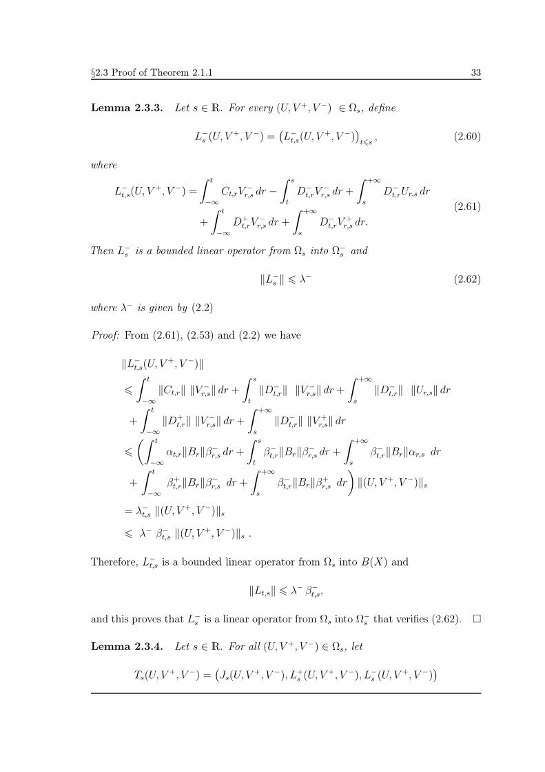
Lemma 2.3.3. Let s ∈ R. For every (U, V +, V −) ∈ Ωs, define
L−s (U, V
+, V −) =(L−t,s(U, V
+, V −))t6s
, (2.60)
where
L−t,s(U, V
+, V −) =
∫ t
−∞
Ct,rV−r,s dr −
∫ s
t
D−t,rV
−r,s dr +
∫ +∞
s
D−t,rUr,s dr
+
∫ t
−∞
D+t,rV
−r,s dr +
∫ +∞
s
D−t,rV
+r,s dr.
(2.61)
Then L−s is a bounded linear operator from Ωs into Ω−
s and
‖L−s ‖ 6 λ− (2.62)
where λ− is given by (2.2)
Proof: From (2.61), (2.53) and (2.2) we have
‖L−t,s(U, V
+, V −)‖
6
∫ t
−∞
‖Ct,r‖ ‖V −r,s‖ dr +
∫ s
t
‖D−t,r‖ ‖V −
r,s‖ dr +
∫ +∞
s
‖D−t,r‖ ‖Ur,s‖ dr
+
∫ t
−∞
‖D+t,r‖ ‖V −
r,s‖ dr +
∫ +∞
s
‖D−t,r‖ ‖V +
r,s‖ dr
6
(∫ t
−∞
αt,r‖Br‖β−r,s dr +
∫ s
t
β−t,r‖Br‖β
−r,s dr +
∫ +∞
s
β−t,r‖Br‖αr,s dr
+
∫ t
−∞
β+t,r‖Br‖β
−r,s dr +
∫ +∞
s
β−t,r‖Br‖β
+r,s dr
)‖(U, V +, V −)‖s
= λ−t,s ‖(U, V+, V −)‖s
6 λ− β−t,s ‖(U, V
+, V −)‖s .
Therefore, L−t,s is a bounded linear operator from Ωs into B(X) and
‖Lt,s‖ 6 λ− β−t,s,
and this proves that L−s is a linear operator from Ωs into Ω−
s that verifies (2.62).
Lemma 2.3.4. Let s ∈ R. For all (U, V +, V −) ∈ Ωs, let
Ts(U, V+, V −) =
(Js(U, V
+, V −), L+s (U, V
+, V −), L−s (U, V
+, V −))

34 Chapter 2: Robustness
where Js, L+s and L−
s are defined by (2.54), (2.57) and (2.60) respectively. Then Ts
is a linear operator from Ωs into Ωs such that
‖Ts‖ 6 maxλ, λ+, λ−
< 1.
Proof: It is obvious considering Lemmas 2.3.1, 2.3.2 and 2.3.3.
Lemma 2.3.5. Let s ∈ R. Then there exists a unique (U, V +, V −) ∈ Ωs such that
Ut,s =Tt,sPs + Jt,s(U, V+, V −) for all (t, s) ∈ R2, (2.63)
V +t,s = Tt,sQ
+s + L+
t,s(U, V+, V −) for all (t, s) ∈ R2
>, (2.64)
V −t,s = Tt,sQ
−s + L−
t,s(U, V+, V −) for all (t, s) ∈ R2
6. (2.65)
Moreover,
‖Ut,s‖ 6 σ αt,s for every (t, s) ∈ R2,
‖V +t,s‖ 6 σ β+
t,s for every (t, s) ∈ R2>
and
‖V −t,s‖ 6 σ β−
t,s for every (t, s) ∈ R26,
where σ =1
1−max λ, λ−, λ+.
Proof: Let s ∈ R and define Γs by
Γs =((Tt,sPs)t∈R, (Tt,sQ
+s )t>s, (Tt,sQ
−s )t6s
).
Then, considering (D1), (D2) and (D3), we can say that Γs ∈ Ωs and ‖Γs‖s 6 1.
Let Υs : Ωs → Ωs be the operator defined by
Υs = Γs + Ts.
Since Ts is a linear contraction with Lipschitz constant max λ, λ+, λ−, Υs is also
a contraction with the same Lipschitz constant. Therefore, since Ωs is a Banach

§2.3 Proof of Theorem 2.1.1 35
space, by the Banach fixed point Theorem, Υs has a unique fixe point, that we will
call (U, V +, V −) and obviously verifies (2.63), (2.64) and (2.65).
Also from the proof of the Banach fixed point Theorem, we have
‖(U, V +, V −)− (0, 0, 0)‖s 6 σ‖Υs(0, 0, 0)− (0, 0, 0)||s = σ‖Γs‖s 6 σ.
Considering the definition of ‖ · ‖s, we have ‖Ut,s‖ 6 σαt,s for every (t, s) ∈ R2,
‖V +t,s‖ 6 σβ+
t,s for every (t, s) ∈ R2> and ‖V −
t,s‖ 6 σβ−t,s for every (t, s) ∈ R2
6.
Lemma 2.3.6. Let s ∈ R. The point (U, V +, V −) ∈ Ωs is a solution of the
equation (2.1).
Proof: From (2.63) and (2.55), for all (t, s) ∈ R2, we have
Ut,s = Tt,sPs −
∫ s
−∞
Ct,rV−r,s dr +
∫ t
s
Ct,rUr,s dr −
∫ +∞
t
D−t,rUr,s dr
+
∫ t
−∞
D+t,rUr,s dr +
∫ +∞
s
Ct,rV+r,s dr.
Noting that the right-hand of (2.63) is differentiable in t, then
∂Ut,s
∂t= v′(t)Ps − v′(t)
∫ s
−∞
PrBrV−r,s dr + v′(t)
∫ t
s
PrBrUr,s dr
+ PtBtUt,s − v′(t)
∫ +∞
t
Q−r BrUr,s dr +Q−
t BtUt,s
+ v′(t)
∫ t
−∞
Q+r BrUr,s dr +Q+
t BtUt,s + v′(t)
∫ +∞
s
PrBrV+r,s dr
= AtTt,sPs − At
∫ s
−∞
Ct,rV−r,s dr + At
∫ t
s
Ct,rUr,s dr
+ PtBtUt,s − At
∫ +∞
t
D−t,rUr,s dr +Q−
t BtUt,s
+ At
∫ t
−∞
D+t,rUr,s dr +Q+
t BtUt,s + At
∫ +∞
s
Ct,rV+r,s dr
= AtUt,s + PtBtUt,s +Q−t BtUt,s +Q+
t BtUt,s
= AtUt,s +BtUt,s
= (At +Bt)Ut,s.

36 Chapter 2: Robustness
In a similar way, from (2.64) and (2.58) we have for all (t, s) ∈ R2>,
V +t,s = Tt,sQ
+s −
∫ s
−∞
D+t,rUr,s dr +
∫ t
s
D+t,rV
+r,s dr −
∫ +∞
t
Ct,rV+r,s dr
−
∫ s
−∞
D+t,rV
−r,s dr −
∫ +∞
t
D−t,rV
+r,s dr
and
∂V +t,s
∂t= AtTt,sQ
+s − v′(t)
∫ s
−∞
Q+r BrUr,s dr + v′(t)
∫ t
s
Q+r BrV
+r,s dr
+Q+t BtV
+t,s − v′(t)
∫ +∞
t
PrBrV+r,s dr + PtBtV
+t,s
− v′(t)
∫ s
−∞
Q+r BrV
−r,s dr − v′(t)
∫ +∞
t
Q−r BrV
+r,s dr +Q−
t BtV+t,s
= (At +Bt)V+t,s.
Finally, from (2.65) and (2.61) we have that
V −t,s = Tt,sQ
−s +
∫ t
−∞
Ct,rV−r,s dr −
∫ s
t
D−t,rV
−r,s dr +
∫ +∞
s
D−t,rUr,s dr
+
∫ t
−∞
D+t,rV
−r,s dr +
∫ +∞
s
D−t,rV
+r,s dr
for all (t, s) ∈ R26 and so
∂V −t,s
∂t= AtTt,sQ
−s + v′(t)
∫ t
−∞
PrBrV−r,s dr + PtBtV
−t,s
− v′(t)
∫ s
t
Q−r BrV
−r,s dr +Q−
t BtV−t,s + v′(t)
∫ +∞
s
Q−r BrUr,s dr
+ v′(t)
∫ t
−∞
Q+r BrV
−r,s dr +Q+
t BtV−t,s + v′(t)
∫ +∞
s
Q−r BrV
+r,s dr
= AtV−t,s +BtV
−t,s
= (At +Bt) V−t,s
and this completes the proof.
Lemma 2.3.7. Let (t, s) ∈ R2. Then we have
Uℓ,s = Uℓ,tUt,s for every (ℓ, t) ∈ R2,
V +ℓ,tUt,s = 0 for every (ℓ, t) ∈ R2
>,
V −ℓ,tUt,s = 0 for every (ℓ, t) ∈ R2
6.

§2.3 Proof of Theorem 2.1.1 37
Proof: Let (t, s) ∈ R2 and define
Wℓ,t = Uℓ,tUt,s − Uℓ,s , (ℓ, t) ∈ R2
Z+ℓ,t = V +
ℓ,tUt,s, (ℓ, t) ∈ R2>
Z−ℓ,t = V −
ℓ,tUt,s , (ℓ, t) ∈ R26.
We must prove that
W = (Wℓ,t)ℓ∈R ∈ Ω0t , Z+ =
(Z+
ℓ,t
)ℓ>t
∈ Ω+t and Z− =
(Z−
ℓ,t
)ℓ6t
∈ Ω−t .
From
‖Wℓ,t‖ 6 ‖Uℓ,t‖‖Ut,s‖+ ‖Uℓ,s‖ 6 σ αℓ,t‖Ut,s‖+ σ αℓ,s 6 σ αℓ,t
(‖Ut,s‖+
αℓ,s
αℓ,t
)
and using (2.6) it follows that W ∈ Ω0t . On the other hand, for every (ℓ, t) ∈ R2
> we
have
‖Z+ℓ,t‖ 6 ‖V +
ℓ,t‖ ‖Ut,s‖ 6 σ β+ℓ,t‖Ut,s‖.
Clearly we have Z+ ∈ Ω+t . Finally, since for every (ℓ, t) ∈ R2
6
‖Z−ℓ,t‖ 6 ‖V −
ℓ,t‖ ‖Ut,s‖ 6 σ β−ℓ,t‖Ut,s‖,
then Z− ∈ Ω−t . Hence (W,Z+, Z−) ∈ Ωt. Now we have to prove that (W,Z+, Z−)
is a fixed point of Tt. From (2.63), for every (ℓ, t) ∈ R2, we have
Wℓ,t = Uℓ,tUt,s − Uℓ,s = Tℓ,tPtUt,s + Jℓ,t(U, V+, V −)Ut,s − Uℓ,s
and since
Tℓ,tPtUt,s = Tℓ,sPs −
∫ s
−∞
Cℓ,rV−r,s dr +
∫ t
s
Cℓ,rUr,s dr +
∫ +∞
s
Cℓ,rV+r,s dr
we have
Tℓ,tPtUt,s − Uℓ,s = −
∫ ℓ
t
Cℓ,rUr,s dr +
∫ +∞
ℓ
D−ℓ,rUr,s dr −
∫ ℓ
−∞
D+ℓ,rUr,s dr

38 Chapter 2: Robustness
and this implies
Wℓ,t = Jℓ,t(W,Z+, Z−).
On the other hand, from (2.64)
Z+ℓ,t = V +
ℓ,tUt,s = Tℓ,tQ+t Ut,s + L+
ℓ,t(U, V+, V −)Ut,s
and because
Tℓ,tQ+t Ut,s =
∫ t
−∞
D+ℓ,rUr,s dr,
we have
Z+ℓ,t = L+
ℓ,t(W,Z+, Z−).
Finally, using (2.65)
Z−ℓ,t = V −
ℓ,tUt,s = Tℓ,tQ−t Ut,s + L−
ℓ,t(U, V+, V −)Ut,s
and because
Tℓ,tQ−t Ut,s = −
∫ +∞
t
D−ℓ,rUr,s dr,
we obtain
Z−ℓ,t = L−
ℓ,t(W,Z+, Z−).
Therefore (W,Z+, Z−) is a fixed point of the linear contraction Tt = (Jt, L+t , L
−t )
and since Tt has a unique fixed point, it must be the zero of Ωt. So, we must have
Uℓ,tUt,s = Uℓ,s for every (ℓ, t) ∈ R2,
V +ℓ,tUt,s = 0 for every (ℓ, t) ∈ R2
>,
V −ℓ,tUt,s = 0 for every (ℓ, t) ∈ R2
6.
Lemma 2.3.8. Let (t, s) ∈ R26. Then we have
Uℓ,tV−t,s = 0 for every (ℓ, t) ∈ R2,
V +ℓ,tV
−t,s = 0 for every (ℓ, t) ∈ R2
>,
V −ℓ,s = V −
ℓ,tV−t,s for every (ℓ, t) ∈ R2
6.

§2.3 Proof of Theorem 2.1.1 39
Proof: Let (t, s) ∈ R26 and define
Wℓ,t = Uℓ,tV−t,s for every (ℓ, t) ∈ R2,
Z+ℓ,t = V +
ℓ,tV−t,s for every (ℓ, t) ∈ R2
>,
Z−ℓ,t = V −
ℓ,tV−t,s − V −
ℓ,s for every (ℓ, t) ∈ R26.
Since
‖Wℓ,t‖ 6 ‖Uℓ,t‖ ‖V −t,s‖ 6 σαℓ,t‖V
−t,s‖
we can say that W ∈ Ω0t . From
‖Z+ℓ,t‖ 6 ‖V +
ℓ,t‖ ‖V −t,s‖ 6 σβ+
ℓ,t‖V−t,s‖
it follows Z+ ∈ Ω+t . At last,
‖Z−ℓ,t‖ 6 ‖V −
ℓ,t‖ ‖V −t,s‖+ ‖V −
ℓ,s‖ 6 σβ−ℓ,t‖V
−t,s‖+ σβ−
ℓ,s 6 σβ−ℓ,t
(‖V −
t,s‖+β−ℓ,s
β−ℓ,t
)
and from (2.8) it follows that Z− ∈ Ω−t .
Therefore (W,Z+, Z−) ∈ Ωt. From (2.63) we have
Wℓ,t = Uℓ,tV−t,s = Tℓ,tPtV
−t,s + Jℓ,t(U, V
+, V −)V −t,s
and since
Tℓ,tPtV−t,s =
∫ t
−∞
Cℓ,rV−r,s dr
we have
Wℓ,t = Jℓ,t(W,Z+, Z−).
On the other hand, we have
Z+ℓ,t = V +
ℓ,tV−t,s = Tℓ,tQ
+t V
−t,s + L+
ℓ,t(U, V+, V −)V −
t,s.
But
Tℓ,tQ+t V
−t,s =
∫ t
−∞
D+ℓ,rV
−r,s dr

40 Chapter 2: Robustness
and so we can write
Z+ℓ,t = L+
ℓ,t(W,Z+, Z−).
Finally, for (ℓ, t) ∈ R2> we have
Z−ℓ,t = V −
ℓ,tV−t,s − V −
ℓ,s
= Tℓ,tQ−t V
−t,s + L−
ℓ,t(U, V+, V −)V −
t,s − V −ℓ,s
and because
Tℓ,tQ−t V
−t,s = Tℓ,sQ
−s −
∫ s
t
D−ℓ,rV
−r,s dr +
∫ +∞
s
D−ℓ,rUr,s dr +
∫ +∞
s
D−ℓ,rV
+r,s dr,
we have
Tℓ,tQ−t V
−t,s − V −
ℓ,s = −
∫ ℓ
−∞
Cℓ,rV−r,s dr +
∫ t
ℓ
D−ℓ,rV
−r,s dr −
∫ ℓ
−∞
D+ℓ,rV
−r,s dr
and this implies
Z−ℓ,t = L−
ℓ,t(W,Z+, Z−).
Once more, (W,Z+, Z−) is a fixed point of the linear contraction and since Tt has a
unique fixed point, it must be the zero of Ωt. So, it follows that
Uℓ,tV−t,s = 0 for every (ℓ, t) ∈ R2,
V +ℓ,tV
−t,s = 0 for every (ℓ, t) ∈ R2
>,
V −ℓ,s = V −
ℓ,tV−t,s for every (ℓ, t) ∈ R2
6.
Lemma 2.3.9. Let (t, s) ∈ R2>. Then we have
Uℓ,tV+t,s = 0 for every (ℓ, t) ∈ R2,
V +ℓ,s = V +
ℓ,tV+t,s for every (ℓ, t) ∈ R2
>,
V −ℓ,tV
+ℓ,t = 0 for every (ℓ, t) ∈ R2
6.

§2.3 Proof of Theorem 2.1.1 41
Proof: Let (t, s) ∈ R2> and define
Wℓ,t = Uℓ,tV+t,s for every (ℓ, t) ∈ R2,
Z+ℓ,t = V +
ℓ,tV+t,s − V +
ℓ,s for every (ℓ, t) ∈ R2>,
Z−ℓ,t = V −
ℓ,tV+t,s for every (ℓ, t) ∈ R2
6.
Since
‖Wℓ,t‖ 6 ‖Uℓ,t‖ ‖V +t,s‖ 6 σαℓ,t‖V
+t,s‖
it follows that W ∈ Ω0t . From
‖Z+ℓ,t‖ 6 ‖V +
ℓ,t‖ ‖V +t,s‖+ ‖V +
ℓ,s‖ 6 σβ+ℓ,t‖V
+t,s‖+ σβ+
ℓ,s 6 σβ+ℓ,t
(‖V +
t,s‖+β+ℓ,s
β+ℓ,t
)
and (2.7) it follows that Z+ ∈ Ω+t . At last,
‖Z−ℓ,t‖ 6 ‖V −
ℓ,t‖ ‖V +t,s‖ 6 σβ−
ℓ,t‖V+t,s‖
we have Z− ∈ Ω−t . Therefore (W,Z+, Z−) ∈ Ωt. From (2.63) we have
Wℓ,t = Uℓ,tV+t,s = Tℓ,tPtV
+t,s + Jℓ,t(U, V
+, V −)V +t,s
and since
Tℓ,tPtV+t,s =
∫ +∞
t
Cℓ,rV+r,s dr
we have
Wℓ,t = Jℓ,t(W,Z+, Z−).
On the other hand, for (ℓ, t) ∈ R2>
Z+ℓ,t = V +
ℓ,tV+t,s − V +
ℓ,s = Tℓ,tQ+t V
+t,s + L+
ℓ,t(U, V+, V −)V +
t,s − V +ℓ,s.
But
Tℓ,tQ+t V
+t,s = Tℓ,sQ
+s −
∫ s
−∞
D+ℓ,rUr,s dr +
∫ t
s
D+ℓ,rV
+r,s dr −
∫ s
−∞
D+ℓ,rV
−r,s dr,
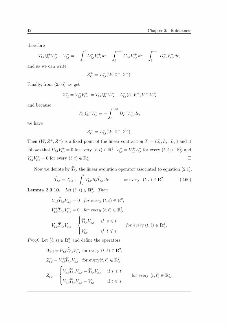
42 Chapter 2: Robustness
therefore
Tℓ,tQ+t V
+t,s − V +
ℓ,s = −
∫ ℓ
t
D+ℓ,rV
+r,s dr −
∫ +∞
ℓ
Cℓ,rV+r,s dr −
∫ +∞
ℓ
D−ℓ,rV
+r,s dr,
and so we can write
Z+ℓ,t = L+
ℓ,t(W,Z+, Z−).
Finally, from (2.65) we get
Z−ℓ,t = V −
ℓ,tV+t,s = Tℓ,tQ
−t V
+t,s + L−
ℓ,t(U, V+, V −)V +
t,s
and because
Tℓ,tQ−t V
+t,s = −
∫ +∞
t
D−ℓ,rV
+r,s dr,
we have
Z−ℓ,t = L−
ℓ,t(W,Z+, Z−).
Then (W,Z+, Z−) is a fixed point of the linear contraction Tt = (Jt, L+t , L
−t ) and it
follows that Uℓ,tV+t,s = 0 for every (ℓ, t) ∈ R2, V +
ℓ,s = V +ℓ,tV
+t,s for every (ℓ, t) ∈ R2
> and
V −ℓ,tV
+ℓ,t = 0 for every (ℓ, t) ∈ R2
6.
Now we denote by Tt,s the linear evolution operator associated to equation (2.1),
Tt,s = Tt,s +
∫ t
s
Tt,rBrTr,s dr for every (t, s) ∈ R2. (2.66)
Lemma 2.3.10. Let (ℓ, s) ∈ R2>. Then
Ut,ℓTℓ,sV−s,s = 0 for every (t, ℓ) ∈ R2,
V +t,ℓTℓ,sV
−s,s = 0 for every (t, ℓ) ∈ R2
>,
V −t,ℓTℓ,sV
−s,s =
Tt,sV
−s,s if s 6 t
V −t,s if t 6 s
for every (t, ℓ) ∈ R26.
Proof: Let (ℓ, s) ∈ R2> and define the operators
Wt,ℓ = Ut,ℓTℓ,sV−s,s for every (t, ℓ) ∈ R2,
Z+t,ℓ = V +
t,ℓTℓ,sV−s,s for every(t, ℓ) ∈ R2
>,
Z−t,ℓ =
V −t,ℓTℓ,sV
−s,s − Tt,sV
−s,s if s 6 t
V −t,ℓTℓ,sV
−s,s − V −
t,s if t 6 s
for every (t, ℓ) ∈ R26.

§2.3 Proof of Theorem 2.1.1 43
It is clear that (W,Z+, Z−) ∈ Ωℓ. For every (t, ℓ) ∈ R2 we can write from (2.63)
Wt,ℓ = Tt,ℓPℓTℓ,sV−s,s + Jt,ℓ(U, V
+, V −)Tℓ,sV−s,s.
But from the definition of T , (2.66), (2.65) and (2.52) we have
Tt,ℓPℓTℓ,sV−s,s = Tt,ℓPℓTℓ,sV
−s,s + Tt,ℓPℓ
∫ ℓ
s
Tℓ,rBrTr,s drV−s,s
= Tt,sPsV−s,s +
∫ ℓ
s
Tt,rPr BrTr,sV−s,s dr
= Tt,sPs
∫ s
−∞
Cs,rV−r,s dr +
∫ ℓ
s
Ct,rTr,sV−s,s dr
=
∫ s
−∞
Ct,rV−r,s dr +
∫ ℓ
s
Ct,rTr,sV−s,s dr.
(2.67)
Since, from (2.55) we have, for every (t, ℓ) ∈ R2
Jt,ℓ(U, V+, V −)Tℓ,sV
−s,s = −
∫ ℓ
−∞
Ct,rV−r,ℓTℓ,sV
−s,s dr +
∫ t
ℓ
Ct,rUr,ℓTℓ,sV−s,s dr
−
∫ +∞
t
D−t,rUr,ℓTℓ,sV
−s,s dr +
∫ t
−∞
D+t,rUr,ℓTℓ,sV
−s,s dr +
∫ +∞
ℓ
Ct,rV+r,ℓTℓ,sV
−s,s dr,
(2.68)
then, from (2.68) and (2.67) we get
Wt,ℓ = Ut,ℓTℓ,sV−s,s
= −
∫ ℓ
−∞
Ct,r(V−r,ℓTℓ,sV
−s,s − Tr,sV
−s,s) dr −
∫ ℓ
s
Ct,rTr,sV−s,s dr +
∫ ℓ
s
Ct,rTr,sV−s,s dr
+
∫ t
ℓ
Ct,rUr,ℓTℓ,sV−s,s dr −
∫ +∞
t
D−t,rUr,ℓTℓ,sV
−s,s dr +
∫ t
−∞
D+t,rUr,ℓTℓ,sV
−s,s dr
+
∫ +∞
ℓ
Ct,rV+r,ℓTℓ,sV
−s,s dr
= −
∫ ℓ
−∞
Ct,rZ−r,ℓ dr +
∫ t
ℓ
Ct,rWr,ℓ dr −
∫ +∞
t
D−t,rWr,ℓ dr
+
∫ t
−∞
D+t,rWr,ℓ dr +
∫ +∞
ℓ
Ct,rZ+r,ℓ dr
= Jt,ℓ(W,Z+, Z−).
For every (t, ℓ) ∈ R2>, using (2.64) we can write
Z+t,ℓ = V +
t,ℓTℓ,sV−s,s = Tt,ℓQ
+ℓ Tℓ,sV
−s,s + L+
t,ℓ(U, V+, V −)Tℓ,sV
−s,s

44 Chapter 2: Robustness
and by (2.66)
Tt,ℓQ+ℓ Tℓ,sV
−s,s = Tt,ℓQ
+ℓ Tℓ,sV
−s,s + Tt,ℓQ
+ℓ
∫ ℓ
s
Tℓ,rBrTr,sV−s,s dr
= Tt,sQ+s V
−s,s +
∫ ℓ
s
Tt,rQ+r BrTr,sV
−s,s dr
= Tt,sQ+s V
−s,s +
∫ ℓ
s
D+t,rTr,sV
−s,s dr
=
∫ s
−∞
D+t,rV
−r,s dr +
∫ ℓ
s
D+t,rTr,sV
−s,s dr.
From (2.58) we get
L+t,ℓ(U, V
+, V −)Tℓ,sV−s,s =−
∫ ℓ
−∞
D+t,rUr,ℓTℓ,sV
−s,s dr +
∫ t
ℓ
D+t,rV
+r,ℓTℓ,sV
−s,s dr
−
∫ +∞
t
Ct,rV+r,ℓTℓ,sV
−s,s dr −
∫ ℓ
−∞
D+t,rV
−r,ℓTℓ,sV
−s,s dr
−
∫ +∞
t
D−t,rV
+r,ℓTℓ,sV
−s,s dr
and so
Z+t,ℓ = Tt,ℓQ
+ℓ Tℓ,sV
−s,s + L+
t,ℓ(U, V+, V −)Tℓ,sV
−s,s
=
∫ s
−∞
D+t,rV
−r,s dr +
∫ ℓ
s
D+t,rTr,sV
−s,s dr −
∫ ℓ
−∞
D+t,rUr,ℓTℓ,sV
−s,s dr
+
∫ t
ℓ
D+t,rV
+r,ℓTℓ,sV
−s,s dr −
∫ +∞
t
Ct,rV+r,ℓTℓ,sV
−s,s dr
−
∫ ℓ
−∞
D+t,rV
−r,ℓTℓ,sV
−s,s dr −
∫ +∞
t
D−t,rV
+r,ℓTℓ,sV
−s,s dr
= −
∫ ℓ
−∞
D+t,rWr,ℓ dr +
∫ t
ℓ
D+t,rZ
+r,ℓ dr −
∫ +∞
t
Ct,rZ+r,ℓ dr
−
∫ ℓ
−∞
D+t,rZ
−r,ℓ dr −
∫ ℓ
−∞
D+t,rTr,sV
−s,s dr −
∫ +∞
t
D−t,rZ
+r,ℓ dr
+
∫ s
−∞
D+t,rV
−r,s dr +
∫ ℓ
s
D+t,rTr,sV
−s,s dr
= L+t,ℓ(W,Z
+, Z−)
For every (t, ℓ) ∈ R26, considering that t 6 s and from (2.65) we have
Z−t,ℓ = V −
t,ℓTℓ,sV−s,s − V −
t,s =Tt,ℓQ−ℓ Tℓ,sV
−s,s + L−
t,ℓ(U, V+, V −)Tℓ,sV
−s,s − V −
t,s,

§2.3 Proof of Theorem 2.1.1 45
from (2.66) it follows that
Tt,ℓQ−ℓ Tℓ,sV
−s,s = Tt,ℓQ
−ℓ Tℓ,sV
−s,s + Tt,ℓQ
−ℓ
∫ ℓ
s
Tℓ,rBrTr,sV−s,s dr
= Tt,sQ−s V
−s,s +
∫ ℓ
s
D−t,rTr,sV
−s,s dr
and by (2.61) we have
L−t,ℓ(U, V
+, V −)Tℓ,sV−s,s =
=
∫ t
−∞
Ct,rV−r,ℓTℓ,sV
−s,s dr −
∫ ℓ
t
D−t,rV
−r,ℓTℓ,sV
−s,s dr +
∫ +∞
ℓ
D−t,rUr,ℓTℓ,sV
−s,s dr
+
∫ t
−∞
D+t,rV
−r,ℓTℓ,sV
−s,s dr +
∫ +∞
ℓ
D−t,rV
+r,ℓTℓ,sV
−s,s dr.
(2.69)
From (2.66) and the definition (2.65) for every s ∈ R we can write
Tt,ℓQ−ℓ Tℓ,sV
−s,s − V −
t,s
= Tt,sQ−s V
−s,s +
∫ ℓ
s
D−t,rTr,sV
−s,s dr − Tt,sQ
−s −
∫ t
−∞
Ct,rV−r,s dr
+
∫ s
t
D−t,rV
−r,s dr −
∫ +∞
s
D−t,rUr,s dr −
∫ t
−∞
D+t,rV
−r,s dr −
∫ +∞
s
D−t,rV
+r,s dr
= Tt,sQ−s +
∫ +∞
s
Tt,sQ−s D
−s,rUr,s dr +
∫ +∞
s
Tt,sQ−s D
−s,rV
+r,s dr
+
∫ ℓ
s
D−t,rTr,sV
−s,s dr − Tt,sQ
−s −
∫ t
−∞
Ct,rV−r,s dr +
∫ s
t
D−t,rV
−r,s dr
−
∫ +∞
s
D−t,rUr,s dr −
∫ t
−∞
D+t,rV
−r,s dr −
∫ +∞
s
D−t,rV
+r,s dr
=
∫ +∞
s
D−t,rUr,s dr +
∫ +∞
s
D−t,rV
+r,s dr +
∫ ℓ
s
D−t,rTr,sV
−s,s dr −
∫ t
−∞
Ct,rV−r,s dr
+
∫ s
t
D−t,rV
−r,s dr −
∫ +∞
s
D−t,rUr,s dr −
∫ t
−∞
D+t,rV
−r,s dr −
∫ +∞
s
D−t,rV
+r,s dr
=
∫ ℓ
s
D−t,rTr,sV
−s,s dr −
∫ t
−∞
Ct,rV−r,s dr +
∫ s
t
D−t,rV
−r,s dr −
∫ t
−∞
D+t,rV
−r,s dr
(2.70)

46 Chapter 2: Robustness
Therefore from (2.69) and (2.70) we have, for every t 6 s 6 ℓ,
Z−t,ℓ
= V −t,ℓTℓ,sV
−s,s − V −
t,s
=
∫ t
−∞
Ct,r
(V −r,ℓTℓ,sV
−s,s − Tr,sV
−s,s
)dr −
∫ ℓ
t
D−t,r
(V −r,ℓTℓ,sV
−s,s − Tr,sV
−s,s
)dr
+
∫ s
ℓ
D−t,rTr,sV
−s,s dr +
∫ +∞
ℓ
D−t,rUr,ℓTℓ,sV
−s,s dr +
∫ t
−∞
D+t,r
(V −r,ℓTℓ,sV
−s,s − V −
r,s
)dr
+
∫ +∞
ℓ
D−t,rV
+r,ℓTℓ,sV
−s,s dr +
∫ ℓ
s
D−t,rTr,sV
−s,s dr
=
∫ t
−∞
Ct,rZ−r,ℓ dr −
∫ ℓ
t
D−t,rZ
−r,ℓ dr +
∫ +∞
ℓ
D−t,rWr,ℓ dr +
∫ t
−∞
D+t,rZ
−r,ℓ dr
+
∫ +∞
ℓ
D−t,rZ
+r,ℓ dr
= L−t,ℓ(W,Z
+, Z−).
Now for every (t, ℓ) ∈ R26, considering s 6 t we have
Z−t,ℓ = V −
t,ℓTℓ,sV−s,s − Tt,sV
−s,s = Tt,ℓQ
−ℓ Tℓ,sV
−s,s + L−
t,ℓ(U, V+, V −)Tℓ,sV
−s,s − Tt,sV
−s,s,

§2.3 Proof of Theorem 2.1.1 47
from (2.66) and (2.65) it follows that, for every s ∈ R,
Tt,ℓQ−ℓ Tℓ,sV
−s,s − Tt,sV
−s,s =
=
(Tt,ℓQ
−ℓ Tℓ,s + Tt,ℓQ
−ℓ
∫ ℓ
s
Tℓ,rBrTr,s dr − Tt,s −
∫ t
s
Tt,rBrTr,s dr
)V −s,s
=
(Tt,sQ
−s +
∫ ℓ
s
D−t,rTr,s dr − Tt,s −
∫ t
s
Tt,rBrTr,s dr
)V −s,s
=
(−Tt,sPs − Tt,sQ
+s +
∫ ℓ
s
D−t,rTr,s dr −
∫ t
s
Tt,rBrTr,s dr
)V −s,s
= −Tt,sPsV−s,s − Tt,sQ
+s V
−s,s +
∫ ℓ
s
D−t,rTr,sV
−s,s dr −
∫ t
s
Tt,rBrTr,sV−s,s dr
= −
∫ s
−∞
Tt,sPsCs,rV−r,s dr −
∫ s
−∞
Tt,sQ+s D
+s,rV
−r,s dr +
∫ ℓ
s
D−t,rTr,sV
−s,s dr
−
∫ t
s
Tt,rBrTr,sV−s,s dr
= −
∫ s
−∞
Ct,rV−r,s dr −
∫ s
−∞
D+t,rV
−r,s dr +
∫ ℓ
s
D−t,rTr,sV
−s,s dr
−
∫ t
s
Tt,rBrTr,sV−s,s dr
and by (2.61) we also have (2.69). Therefore from (2.69) and (2.70) we have, for

48 Chapter 2: Robustness
every s 6 t 6 ℓ,
Z−t,ℓ = V −
t,ℓTℓ,sV−s,s − Tt,sV
−s,s
=
∫ t
−∞
Ct,r
(V −r,ℓTℓ,sV
−s,s − Tr,sV
−s,s
)dr +
∫ t
−∞
Ct,rTr,sV−s,s dr
−
∫ ℓ
t
D−t,r
(V −r,ℓTℓ,sV
−s,s − Tr,sV
−s,s
)dr +
∫ t
s
D−t,rTr,sV
−s,s dr
+
∫ +∞
ℓ
D−t,rUr,ℓTℓ,sV
−s,s dr +
∫ t
−∞
D+t,r
(V −r,ℓTℓ,sV
−s,s − Tr,sV
−s,s
)dr
+
∫ t
−∞
D+t,rTr,sV
−s,s dr +
∫ +∞
ℓ
D−t,rV
+r,ℓTℓ,sV
−s,s dr −
∫ s
−∞
Ct,rV−r,s dr
−
∫ s
−∞
D+t,rV
−r,s dr −
∫ t
s
Tt,rBrTr,sV−s,s dr
=
∫ t
−∞
Ct,rZ−r,ℓ dr −
∫ ℓ
t
D−t,rZ
−r,ℓ dr +
∫ +∞
ℓ
D−t,rWr,ℓ dr +
∫ t
−∞
D+t,rZ
−r,ℓ dr
+
∫ +∞
ℓ
D−t,rZ
+r,ℓ dr +
∫ t
−∞
Ct,rTr,sV−s,s dr −
∫ s
−∞
Ct,rV−r,s dr
+
∫ t
s
D−t,rTr,sV
−s,s dr −
∫ s
−∞
D+t,rV
−r,s dr +
∫ t
−∞
D+t,rTr,sV
−s,s dr
−
∫ t
s
Tt,r(Pr +Q+r +Q−
r )BrTr,sV−s,s dr
= L−t,ℓ(W,Z
+, Z−).
Therefore, (W,Z+, Z−) is a fixed point of Tℓ = (Jℓ, L+ℓ , L
−ℓ ), a linear operator. It
follows Wt,ℓ = 0 for every (t, ℓ) ∈ R2, Z−t,ℓ = 0 for every (t, ℓ) ∈ R2
6 and Z+t,ℓ = 0 for
every (t, ℓ) ∈ R2>.
Lemma 2.3.11. Let (ℓ, s) ∈ R26. Then
Ut,ℓTℓ,sV+s,s = 0 for every (t, ℓ) ∈ R2,
V −t,ℓTℓ,sV
+s,s = 0 for every (t, ℓ) ∈ R2
6,
V +t,ℓTℓ,sV
+s,s =
Tt,sV
+s,s if t 6 s
V +t,s if t > s
for every (t, ℓ) ∈ R2>.

§2.3 Proof of Theorem 2.1.1 49
Proof: Let (ℓ, s) ∈ R26 and define the operators
Wt,ℓ = Ut,ℓTℓ,sV+s,s for every (t, ℓ) ∈ R2,
Z−t,ℓ = V −
t,ℓTℓ,sV+s,s for every (t, ℓ) ∈ R2
6,
Z+t,ℓ =
V +t,ℓTℓ,sV
+s,s − Tt,sV
+s,s if t 6 s
V +t,ℓTℓ,sV
+s,s − V +
t,s if t > s
for every (t, ℓ) ∈ R2>.
Obviously (W,Z+, Z−) ∈ Ωℓ. For every (t, ℓ) ∈ R2 we can write from (2.63)
Wt,ℓ = Tt,ℓPℓTℓ,sV+s,s + Jt,ℓ(U, V
+, V −)Tℓ,sV+s,s.
But from the definition of T , (2.66), (2.64) and (2.52) we have
Tt,ℓPℓTℓ,sV+s,s = Tt,ℓPℓTℓ,sV
+s,s + Tt,ℓPℓ
∫ ℓ
s
Tℓ,rBrTr,s drV+s,s
= Tt,sPsV+s,s +
∫ ℓ
s
Tt,rPr BrTr,sV+s,s dr
= −Tt,sPs
∫ +∞
s
Cs,rV+r,s dr +
∫ ℓ
s
Ct,rTr,sV+s,s dr
= −
∫ +∞
s
Ct,rV+r,s dr +
∫ ℓ
s
Ct,rTr,sV+s,s dr.
(2.71)
Since, from (2.55) we have, for every (t, ℓ) ∈ R2
Jt,ℓ(U, V+, V −)Tℓ,sV
+s,s =
= −
∫ ℓ
−∞
Ct,rV−r,ℓTℓ,sV
+s,s dr +
∫ t
ℓ
Ct,rUr,ℓTℓ,sV+s,s dr −
∫ +∞
t
D−t,rUr,ℓTℓ,sV
+s,s dr
+
∫ t
−∞
D+t,rUr,ℓTℓ,sV
+s,s dr +
∫ +∞
ℓ
Ct,rV+r,ℓTℓ,sV
+s,s dr,
(2.72)
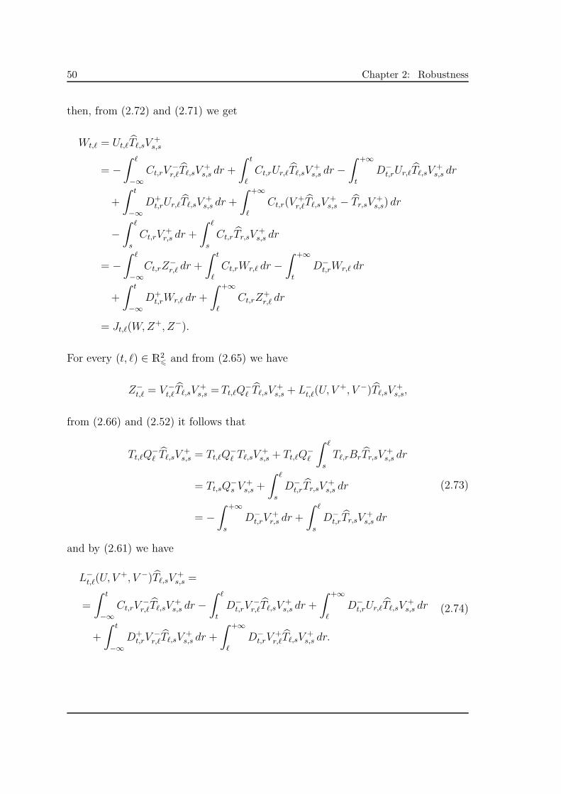
50 Chapter 2: Robustness
then, from (2.72) and (2.71) we get
Wt,ℓ = Ut,ℓTℓ,sV+s,s
= −
∫ ℓ
−∞
Ct,rV−r,ℓTℓ,sV
+s,s dr +
∫ t
ℓ
Ct,rUr,ℓTℓ,sV+s,s dr −
∫ +∞
t
D−t,rUr,ℓTℓ,sV
+s,s dr
+
∫ t
−∞
D+t,rUr,ℓTℓ,sV
+s,s dr +
∫ +∞
ℓ
Ct,r(V+r,ℓTℓ,sV
+s,s − Tr,sV
+s,s) dr
−
∫ ℓ
s
Ct,rV+r,s dr +
∫ ℓ
s
Ct,rTr,sV+s,s dr
= −
∫ ℓ
−∞
Ct,rZ−r,ℓ dr +
∫ t
ℓ
Ct,rWr,ℓ dr −
∫ +∞
t
D−t,rWr,ℓ dr
+
∫ t
−∞
D+t,rWr,ℓ dr +
∫ +∞
ℓ
Ct,rZ+r,ℓ dr
= Jt,ℓ(W,Z+, Z−).
For every (t, ℓ) ∈ R26 and from (2.65) we have
Z−t,ℓ = V −
t,ℓTℓ,sV+s,s = Tt,ℓQ
−ℓ Tℓ,sV
+s,s + L−
t,ℓ(U, V+, V −)Tℓ,sV
+s,s,
from (2.66) and (2.52) it follows that
Tt,ℓQ−ℓ Tℓ,sV
+s,s = Tt,ℓQ
−ℓ Tℓ,sV
+s,s + Tt,ℓQ
−ℓ
∫ ℓ
s
Tℓ,rBrTr,sV+s,s dr
= Tt,sQ−s V
+s,s +
∫ ℓ
s
D−t,rTr,sV
+s,s dr
= −
∫ +∞
s
D−t,rV
+r,s dr +
∫ ℓ
s
D−t,rTr,sV
+s,s dr
(2.73)
and by (2.61) we have
L−t,ℓ(U, V
+, V −)Tℓ,sV+s,s =
=
∫ t
−∞
Ct,rV−r,ℓTℓ,sV
+s,s dr −
∫ ℓ
t
D−t,rV
−r,ℓTℓ,sV
+s,s dr +
∫ +∞
ℓ
D−t,rUr,ℓTℓ,sV
+s,s dr
+
∫ t
−∞
D+t,rV
−r,ℓTℓ,sV
+s,s dr +
∫ +∞
ℓ
D−t,rV
+r,ℓTℓ,sV
+s,s dr.
(2.74)

§2.3 Proof of Theorem 2.1.1 51
Therefore, from (2.73) and (2.74) we have, for every t 6 ℓ,
Z−t,ℓ = V −
t,ℓTℓ,sV+s,s
= −
∫ +∞
s
D−t,rV
+r,s dr +
∫ t
−∞
Ct,rV−r,ℓTℓ,sV
+s,s dr −
∫ ℓ
t
D−t,rV
−r,ℓTℓ,sV
+s,s dr
+
∫ +∞
ℓ
D−t,rUr,ℓTℓ,sV
+s,s dr +
∫ t
−∞
D+t,rV
−r,ℓTℓ,sV
+s,s dr
+
∫ +∞
ℓ
D−t,r(V
+r,ℓTℓ,sV
+s,s − Tr,sV
+s,s) dr +
∫ +∞
ℓ
D−t,rTr,sV
+s,s dr
+
∫ ℓ
s
D−t,rTr,sV
+s,s dr
= −
∫ +∞
s
D−t,rV
+r,s dr +
∫ t
−∞
Ct,rZ−r,ℓ dr −
∫ ℓ
t
D−t,rZ
−r,ℓ dr +
∫ +∞
ℓ
D−t,rWr,ℓ dr
+
∫ t
−∞
D+t,rZ
−r,ℓ dr +
∫ +∞
ℓ
D−t,rZ
+r,ℓ dr +
∫ +∞
ℓ
D−t,rTr,sV
+s,s dr
+
∫ ℓ
s
D−t,rTr,sV
+s,s dr
= L−t,ℓ(W,Z
+, Z−).
At last, for every (t, ℓ) ∈ R2>, supposing t > s and using (2.64) we can write
Z+t,ℓ = V +
t,ℓTℓ,sV+s,s − V +
t,s = Tt,ℓQ+ℓ Tℓ,sV
+s,s + L+
t,ℓ(U, V+, V −)Tℓ,sV
+s,s − V +
t,s
and by (2.66) and (2.64) we have
Tt,ℓQ+ℓ Tℓ,sV
+s,s = Tt,ℓQ
+ℓ Tℓ,sV
+s,s + Tt,ℓQ
+ℓ
∫ ℓ
s
Tℓ,rBrTr,sV+s,s dr
= Tt,sQ+s V
+s,s +
∫ ℓ
s
Tt,rQ+r BrTr,sV
+s,s dr
= Tt,sQ+s V
+s,s +
∫ ℓ
s
D+t,rTr,sV
+s,s dr
= Tt,sQ+s −
∫ s
−∞
D+t,rUr,s dr −
∫ s
−∞
D+t,rV
−r,s dr +
∫ ℓ
s
D+t,rTr,sV
+s,s dr.

52 Chapter 2: Robustness
Therefore we can put
Tt,ℓQ+ℓ Tℓ,sV
+s,s − V +
t,s =
= Tt,sQ+s −
∫ s
−∞
D+t,rUr,s dr −
∫ s
−∞
D+t,rV
−r,s dr +
∫ ℓ
s
D+t,rTr,sV
+s,s dr − Tt,sQ
+s
+
∫ s
−∞
D+t,rUr,s dr −
∫ t
s
D+t,rV
+r,s dr +
∫ +∞
t
Ct,rV+r,s dr +
∫ s
−∞
D+t,rV
−r,s dr
+
∫ +∞
t
D−t,rV
+r,s dr
=
∫ ℓ
s
D+t,rTr,sV
+s,s dr −
∫ t
s
D+t,rV
+r,s dr +
∫ +∞
t
Ct,rV+r,s dr +
∫ +∞
t
D−t,rV
+r,s dr.
From (2.58) we get
L+t,ℓ(U, V
+, V −)Tℓ,sV+s,s =
= −
∫ ℓ
−∞
D+t,rUr,ℓTℓ,sV
+s,s dr +
∫ t
ℓ
D+t,rV
+r,ℓTℓ,sV
+s,s dr −
∫ +∞
t
Ct,rV+r,ℓTℓ,sV
+s,s dr
−
∫ ℓ
−∞
D+t,rV
−r,ℓTℓ,sV
+s,s dr −
∫ +∞
t
D−t,rV
+r,ℓTℓ,sV
+s,s dr
and therefore
Z+t,ℓ =
∫ ℓ
s
D+t,rTr,sV
+s,s dr −
∫ t
s
D+t,rV
+r,s dr +
∫ +∞
t
Ct,rV+r,s dr
+
∫ +∞
t
D−t,rV
+r,s dr −
∫ ℓ
−∞
D+t,rUr,ℓTℓ,sV
+s,s dr +
∫ t
ℓ
D+t,rV
+r,ℓTℓ,sV
+s,s dr
−
∫ +∞
t
Ct,rV+r,ℓTℓ,sV
+s,s dr −
∫ ℓ
−∞
D+t,rV
−r,ℓTℓ,sV
+s,s dr
−
∫ +∞
t
D−t,rV
+r,ℓTℓ,sV
+s,s dr
= −
∫ ℓ
−∞
D+t,rWr,ℓ dr +
∫ t
ℓ
D+t,r(V
+r,ℓTℓ,sV
+s,s − Tr,sV
+s,s) dr +
∫ s
ℓ
D+t,rTr,sV
+s,s dr
−
∫ +∞
t
Ct,rZ+r,ℓ dr −
∫ ℓ
−∞
D+t,rZ
−r,ℓ dr −
∫ +∞
t
D−t,rZ
+r,ℓ dr
+
∫ ℓ
s
D+t,rTr,sV
+s,s dr
= L+t,ℓ(W,Z
+, Z−).

§2.3 Proof of Theorem 2.1.1 53
Finally, for every (t, ℓ) ∈ R2>, supposing t 6 s and using (2.64) we can write
Z+t,ℓ = V +
t,ℓTℓ,sV+s,s − Tt,sV
+s,s = Tt,ℓQ
+ℓ Tℓ,sV
+s,s + L+
t,ℓ(U, V+, V −)Tℓ,sV
+s,s − Tt,sV
+s,s
and by (2.66) and (2.64) we have
Tt,ℓQ+ℓ Tℓ,sV
+s,s − Tt,sV
+s,s =
= Tt,ℓQ+ℓ Tℓ,sV
+s,s + Tt,ℓQ
+ℓ
∫ ℓ
s
Tℓ,rBrTr,sV+s,s dr − Tt,sV
+s,s −
∫ t
s
Tt,rBrTr,sV+s,s dr
= Tt,sQ+s V
+s,s +
∫ ℓ
s
Tt,rQ+r BrTr,sV
+s,s dr − Tt,sV
+s,s −
∫ t
s
Tt,rBrTr,sV+s,s dr
= (−Tt,sPs − Tt,sQ−s )V
+s,s +
∫ ℓ
s
D+t,rTr,sV
+s,s dr −
∫ t
s
Tt,rBrTr,sV+s,s dr
=
∫ +∞
s
Tt,sPsCs,rV+r,s dr +
∫ +∞
s
Tt,sQ−s D
−s,rV
+r,s dr +
∫ ℓ
s
D+t,rTr,sV
+s,s dr
−
∫ t
s
Tt,r IdBrTr,sV+s,s dr
=
∫ +∞
s
Ct,rV+r,s dr +
∫ +∞
s
D−t,rV
+r,s dr +
∫ ℓ
s
D+t,rTr,sV
+s,s dr
−
∫ t
s
Tt,rPrBrTr,sV+s,s dr −
∫ t
s
Tt,rQ+r BrTr,sV
+s,s dr −
∫ t
s
Tt,rQ−r BrTr,sV
+s,s dr
=
∫ +∞
s
Ct,rV+r,s dr +
∫ +∞
s
D−t,rV
+r,s dr +
∫ ℓ
t
D+t,rTr,sV
+s,s dr
−
∫ t
s
Ct,rTr,sV+s,s dr −
∫ t
s
D−t,rTr,sV
+s,s dr.
From (2.58) we get
L+t,ℓ(U, V
+, V −)Tℓ,sV+s,s =
= −
∫ ℓ
−∞
D+t,rUr,ℓTℓ,sV
+s,s dr +
∫ t
ℓ
D+t,rV
+r,ℓTℓ,sV
+s,s dr −
∫ +∞
t
Ct,rV+r,ℓTℓ,sV
+s,s dr
−
∫ ℓ
−∞
D+t,rV
−r,ℓTℓ,sV
+s,s dr −
∫ +∞
t
D−t,rV
+r,ℓTℓ,sV
+s,s dr

54 Chapter 2: Robustness
and therefore
Z+t,ℓ =
∫ +∞
s
Ct,rV+r,s dr +
∫ +∞
s
D−t,rV
+r,s dr +
∫ ℓ
t
D+t,rTr,sV
+s,s dr
−
∫ t
s
Ct,rTr,sV+s,s dr −
∫ t
s
D−t,rTr,sV
+s,s dr −
∫ ℓ
−∞
D+t,rUr,ℓTℓ,sV
+s,s dr
+
∫ t
ℓ
D+t,rV
+r,ℓTℓ,sV
+s,s dr −
∫ +∞
t
Ct,rV+r,ℓTℓ,sV
+s,s dr
−
∫ ℓ
−∞
D+t,rV
−r,ℓTℓ,sV
+s,s dr −
∫ +∞
t
D−t,rV
+r,ℓTℓ,sV
+s,s dr
= −
∫ ℓ
−∞
D+t,rUr,ℓTℓ,sV
+s,s dr +
∫ t
ℓ
D+t,r(V
+r,ℓTℓ,sV
+s,s − Tr,sV
+s,s) dr
−
∫ +∞
t
Ct,r(V+r,ℓTℓ,sV
+s,s − Tr,sV
+s,s) dr −
∫ +∞
t
Ct,rTr,sV+s,s dr
−
∫ ℓ
−∞
D+t,rV
−r,ℓTℓ,sV
+s,s dr −
∫ +∞
t
D−t,r(V
+r,ℓTℓ,sV
+s,s − Tr,sV
+s,s) dr
−
∫ +∞
t
D−t,rTr,sV
+s,s dr +
∫ +∞
s
Ct,rV+r,s dr +
∫ +∞
s
D−t,rV
+r,s dr
−
∫ t
s
Ct,rTr,sV+s,s dr −
∫ t
s
D−t,rTr,sV
+s,s dr
= L+t,ℓ(W,Z
+, Z−).
Hence, (W,Z+, Z−) is a fixed point of the linear operator Tℓ =(Jℓ, L
+ℓ , L
−ℓ
). It
follows Wt,ℓ = 0 for every (t, ℓ) ∈ R2, Z+t,ℓ = 0 for every (t, ℓ) ∈ R2
> and Z−t,ℓ = 0 for
every (t, ℓ) ∈ R26.
Now we are going to define, for each s ∈ R, the linear subspaces Es = Us,s(X),
F+s = V +
s,s(X) and F−s = V −
s,s(X) and state the following lemma.
Lemma 2.3.12. For every (t, s) ∈ R2 we have
Tt,s(Es) ⊆ Et, Tt,s(F+s ) ⊆ F+
t and Tt,s(F−s ) ⊆ F−
t .
Proof: Let x ∈ Es. Then x = Us,sy for some y ∈ X . Since Us,sUs,s = Us,s then
x = Us,sx. By Lemmas 2.3.6 and 2.3.7
Tt,sx = Tt,sUs,sx = Ut,sx = Ut,tUt,sx

§2.3 Proof of Theorem 2.1.1 55
and so Tt,sx ∈ Et. To prove the second inclusion, let x ∈ F+s . In a similar way, we
have x = V +s,sx. Using Lemmas 2.3.6 and 2.3.9 it follows that
Tt,sx = Tt,sV+s,sx = V +
t,sx = V +t,tV
+t,sx
and so Tt,sx ∈ F+t . At last, let x ∈ F−
s . Then x = V −s,sx. By Lemmas 2.3.6 and 2.3.8
we have
Tt,sx = Tt,sV−s,sx = V −
t,sx = V −t,tV
−t,sx
and so Tt,sx ∈ F−t .
§2.3.2 Proof of Theorem 2.1.1
Setting Ps = Us,s, Q+s = V +
s,s and Q−s = V −
s,s, we can now prove Theorem 2.1.1l.
First of all we need to prove that Ps, Q+s and Q−
s are projections. Attending to (2.63),
(2.64) and (2.65) we have
Ps + Q+s + Q−
s
= Ps + Js,s(U, V+, V −) +Q+
s + L+s,s(U, V
+, V −) +Q−s + L−
s,s(U, V+, V −)
= Ps −
∫ s
−∞
Cs,rV−r,s dr −
∫ +∞
s
D−s,rUr,s dr +
∫ s
−∞
D+s,rUr,s dr
+
∫ +∞
s
Cs,rV+r,s dr +Q+
s −
∫ s
−∞
D+s,rUr,s dr −
∫ +∞
s
Cs,rV+r,s dr
−
∫ s
−∞
D+s,rV
−r,s dr −
∫ +∞
s
D−s,rV
+r,s dr +Q−
s +
∫ s
−∞
Cs,rV−r,s dr
+
∫ +∞
s
D−s,rUr,s dr +
∫ s
−∞
D+s,rV
−r,s dr +
∫ +∞
s
D−s,rV
+r,s dr
= Ps +Q+s +Q−
s
= Id
and by Lemmas 2.3.7, 2.3.8 and 2.3.9 we can say PsPs = Ps, Q+s Q
+s = Q+
s and
Q−s Q
−s = Q−
s . Therefore Ps, Q+s and Q−
s are projections and by Lemma 2.3.9 setting

56 Chapter 2: Robustness
t = ℓ = s we have PsQ+s = 0. By Lemmas 2.3.10 and 2.3.11 we have, for every
t, s ∈ R
Tt,sPs = PtTt,sPs + Q+t Tt,sPs + Q−
t Tt,sPs
= PtTt,s
(Id−Q+
s − Q−s
)+ Q+
t Tt,sPs + Q−t Tt,sPs
= PtTt,s − PtTt,sQ+s − PtTt,sQ
−s + Q+
t Tt,sPs + Q−t Tt,sPs
= PtTt,s.
In a similar way we can say
Tt,sQ+s = Q+
t Tt,s and Tt,sQ−s = Q−
t Tt,s for every t, s ∈ R,
i.e., (S1), (S2), (S3) and (S4) are verified which means that (2.1) has an invariant
splitting. At last, from Lemmas 2.3.5 and 2.3.6 we can write
‖Tt,sPs‖ = ‖Ut,s‖ 6 σαt,s for every (t, s) ∈ R2,
‖Tt,sQ+s ‖ = ‖V +
t,s‖ 6 σβ+t,s for every (t, s) ∈ R2
>,
‖Tt,sQ−s ‖ = ‖V −
t,s‖ 6 σβ−t,s for every (t, s) ∈ R2
6.
Therefore equation (2.1) admits a generalized trichotomy with bounds (σαt,s), (σβ+t,s)
and (σβ−t,s) and this completes the proof.

Chapter 3
Global Lipschitz invariant
manifolds
This chapter is dedicated to the study of the existence of global Lipschitz invari-
ant manifolds when equation (1.1) admits a generalized trichotomy and is submitted
to a nonlinear perturbation f satisfying some conditions, namely a Lipschitz condi-
tion. Here, in section 3.1, we formulate a theorem concerning the existence of center
invariant manifolds considering bounds of a more general form and to prove it we
need to establish some lemmas. We also include, in section 3.2, the exhibition of
some examples of invariant center manifolds. The first example is a new general
case that includes some already existent in the literature, namely the ones done by
Barreira and Valls in [11, 3]. In the last section of this chapter we give the proof of
the theorem stated before in the first section.
The proof of the main theorem of this chapter is based in the so-called classical
Lyapunov-Perron method (see [41, 49]) that consists in the following:
− the variation of constants formula that allows to relate the solutions of the linear
equation with the solutions of the perturbed equation;
− the construction of a suitable space of functions that is a complete metric space;

58 Chapter 3: Global Lipschitz invariant manifolds
− the construction of a suitable contraction on the complete metric space mentioned
above;
− the application of Banach’s fixed point theorem to the mentioned contraction
gives a function that is the only fixed point of the contraction whose graph is the
invariant manifold.
This method was used by many authors, namely by [3, 11, 20, 21]. However we
have introduced a novelty in the application of the method. In [3, 11, 20, 21] uses
two applications of the Banach’s fixed point theorem, the first one to obtain the
solutions of the perturbed equation along the stable/center direction and the other
to obtain the solutions of the perturbed equation in the other directions. Here, with
only one application of the Banach’s fixed point theorem, we obtain the solutions of
the perturbed equation in all the directions.
The results of this chapter are from the preprint Bento and Costa [13].
§3.1 Existence of global Lipschitz invariant manifolds
Suppose that equation (1.1) admits a generalized trichotomy. Consider the initial
value problem
v′ = A(t)v + f(t, v), v(s) = vs (3.1)
where f : R×X → X is a continuous function such that
f(t, 0) = 0 for every t ∈ R (3.2)
and, for every t ∈ R,
Lip (ft) := sup
‖f(t, x)− f(t, y)‖
‖x− y‖: x, y ∈ X, x 6= y
< +∞, (3.3)
i.e., the function ft : X → X given by ft(x) = f(t, x) is a Lipschitz function (in x).
Clearly
‖f(t, x)− f(t, y)‖ 6 Lip (ft) ‖x− y‖ (3.4)

§3.1 Existence of global Lipschitz invariant manifolds 59
for every x, y ∈ X and every t ∈ R and taking y = 0 in the last inequality and
by (3.2), we have
‖f(t, x)‖ 6 Lip (ft) ‖x‖ (3.5)
for every x ∈ X and every t ∈ R.
When (1.1) admits a generalized trichotomy, we can write the only solution
of (3.1) in the form
(x(t, s, vs), y
+(t, s, vs), y−(t, s, vs)
)∈ Et × F+
t × F−t
where vs = (ξ, η+, η−) ∈ Es × F+s × F−
s , then solving problem (3.1) is equivalent to
solve the following problem
x(t) = Tt,sPsξ +
∫ t
s
Tt,rPrf(r, x(r), y+(r), y−(r)) dr (3.6)
y+(t) = Tt,sQ+s η
+ +
∫ t
s
Tt,rQ+r f(r, x(r), y
+(r), y−(r)) dr (3.7)
y−(t) = Tt,sQ−s η
− +
∫ t
s
Tt,rQ−r f(r, x(r), y
+(r), y−(r)) dr (3.8)
for every t ∈ R.
Definition 3.1.1. We define the flow of differential equation (3.1) as
Ψτ(s, vs) =(s+ τ, x(s+ τ, s, vs), y
+(s + τ, s, vs), y−(s+ τ, s, vs)
)(3.9)
for each τ ∈ R.
We are going to study the existence of invariant center manifolds for equa-
tion (3.1) when (1.1) admits a generalized trichotomy. The invariant center mani-
folds that we are going to obtain are given by the graph of a function belonging to
a certain function space that we define now.
For
G = (s, ξ) : s ∈ R, ξ ∈ Es ⊂ R×X

60 Chapter 3: Global Lipschitz invariant manifolds
and N ∈ ]0,+∞[, we denote by AN the space of continuous functions ϕ : G → X
such that
ϕ(t, 0) = 0 for all t ∈ R; (3.10)
ϕ(t, ξ) ∈ F+t ⊕ F−
t for all (t, ξ) ∈ G; (3.11)
sup
∥∥ϕ(t, ξ)− ϕ(t, ξ)∥∥
∥∥ξ − ξ∥∥ : (t, ξ), (t, ξ) ∈ G, ξ 6= ξ
6 N. (3.12)
Note that from (3.12) it follows immediately that
∥∥ϕ(t, ξ)− ϕ(t, ξ)∥∥ 6 N
∥∥ξ − ξ∥∥ for all (t, ξ), (t, ξ) ∈ G, (3.13)
and making ξ = 0 in (3.13), we have
‖ϕ(t, ξ)‖ 6 N ‖ξ‖ for every (t, ξ) ∈ G. (3.14)
By (3.11), and identifying F+t ⊕ F−
t and F+t × F−
t as the same space, we can
write ϕ = (ϕ+, ϕ−), where ϕ+(t, ξ) = Q+t ϕ(t, ξ) and ϕ
−(t, ξ) = Q−t ϕ(t, ξ).
We also define the graph, for all the functions ϕ ∈ AN , as follows.
Definition 3.1.2. Let ϕ ∈ AN . We define the graph of ϕ as
Vϕ = (s, ξ, ϕ(s, ξ)) : (s, ξ) ∈ G
=(s, ξ, ϕ+(s, ξ), ϕ−(s, ξ)
): (s, ξ) ∈ G
⊆ R×X.
(3.15)
Before state the main theorem we need to define the following quantities:
σ := sup(t,s)∈R2
∣∣∣∣∫ t
s
αt,r Lip (fr)αr,s
αt,s
dr
∣∣∣∣ (3.16)
and
ω := sups∈R
[∫ s
−∞
β+s,r Lip (fr)αr,s dr +
∫ +∞
s
β−s,r Lip (fr)αr,s dr
]. (3.17)

§3.2 Examples of invariant center manifolds 61
Theorem 3.1.3. Let X be a Banach space. Suppose that (1.1) admits a generalized
trichotomy with bounds αt,s, β+t,s and β−
t,s and let f : R × X → X be a continuous
function such that (3.2) and (3.3) are satisfied. If
limr→+∞
β−s,rαr,s = lim
r→−∞β+s,rαr,s = 0 for every s ∈ R (3.18)
and
2σ + 2ω < 1,
where σ and ω are given by (3.16) and (3.17), respectively, then there is N ∈ ]0, 1[
and a unique ϕ ∈ AN such that
Ψτ(Vϕ) ⊂ Vϕ
for every τ ∈ R, where Ψτ is given by (3.9) and Vϕ is given by (3.15). Moreover,
∥∥Ψt−s(s, ξ, ϕ(s, ξ))−Ψt−s(s, ξ, ϕ(s, ξ))∥∥ 6
N
ωαt,s
∥∥ξ − ξ∥∥
for all (t, s) ∈ R2 and all ξ, ξ ∈ Es.
The proof of last theorem will be given in Section 3.3.
§3.2 Examples of invariant center manifolds
In this section we will give particular cases of Theorem 3.1.3.
§3.2.1 Nonuniform (a, b, c, d)−trichotomies
In this subsection, we will apply this last result to trichotomies with bounds of
the form (1.4).
Theorem 3.2.1. Let X be a Banach space. Suppose that equation (1.1) admits a
nonuniform (a, b, c, d)−trichotomy and let f : R×X → X be a continuous function

62 Chapter 3: Global Lipschitz invariant manifolds
such that (3.2) and (3.3) are satisfied and
Lip(fr) 6 δmin
1
c(r)d(r)εd(r)
[c(r)d(r)
εc(r)
]′,a(r)b(r)
εb(r)
[−
1
a(r)b(r)εa(r)
]′, γ(r)
(3.19)
for every r ∈ R \ 0, where δ < 1/6 and γ : R→ ]0,+∞[ is a function such that
max
∫ +∞
−∞
εa(r)γ(r) dr,
∫ +∞
−∞
εc(r)γ(r) dr
6 1. (3.20)
If
limr→−∞
c(r)d(r)εd(r) = limr→+∞
εb(r)
a(r)b(r)= 0 (3.21)
then equation (3.1) admits an invariant center manifold, i.e., there is N ∈ ]0, 1[ and
a unique ϕ ∈ AN such that
Ψτ(Vϕ) ⊂ Vϕ for every τ ∈ R,
where Ψτ is given by (3.9) and Vϕ is given by (3.15). Furthermore,
∥∥Ψt−s(ps,ξ)−Ψt−s(ps,ξ)∥∥ 6
N
ω
a(s)
a(t)εa(s)
∥∥ξ − ξ∥∥ if t > s,
N
ω
c(t)
c(s)εc(s)
∥∥ξ − ξ∥∥ if t 6 s,
for all (s, ξ), (s, ξ) ∈ G and where ps,ξ = (s, ξ, ϕ(s, ξ)) and ps,ξ =(s, ξ, ϕ(s, ξ)
).
Proof: It is obvious that for this type of bounds (3.18) is equivalent to (3.21). More-
over, since
αt,rαr,s
αt,s=
a(r)/a(t) εa(r) a(s)/a(r) εa(s)
a(s)/a(t) εa(s)if t > r > s,
c(t)/c(r) εc(r) c(r)/c(s) εc(s)
c(t)/c(s) εc(s)if t 6 r 6 s,
=
εa(r) if t > r > s,
εc(r) if t 6 r 6 s,

§3.2 Examples of invariant center manifolds 63
from (3.19) and (3.20) we have
σ = sup(t,s)∈R2
∣∣∣∣∫ t
s
αt,r Lip(fr)αr,s
αt,sdr
∣∣∣∣
= max
sup
(t,s)∈R2
>
∫ t
s
εa(r) Lip(fr) dr, sup(t,s)∈R2
6
∫ s
t
εc(r) Lip(fr) dr
= max
∫ +∞
−∞
εa(r) Lip(fr) dr,
∫ +∞
−∞
εc(r) Lip(fr) dr
6 δmax
∫ +∞
−∞
εa(r)γ(r) dr,
∫ +∞
−∞
εc(r)γ(r) dr
6 δ.
From (3.19) and (3.21) it follows that
ω = sups∈R
[∫ s
−∞
β+s,r Lip (fr)αr,s dr +
∫ +∞
s
β−s,r Lip (fr)αr,s dr
]
= sups∈R
[∫ s
−∞
d(r)εd(r)c(r)εc(s)
d(s)c(s)Lip(fr) dr +
∫ +∞
s
b(s)εb(r)a(s)εa(s)
b(r)a(r)Lip(fr) dr
]
6 δ
[εc(s)
c(s)d(s)
∫ s
−∞
(c(r)d(r)
εc(r)
)′
dr − a(s)b(s)εa(s)
∫ +∞
s
(1
a(r)b(r)εa(r)
)′
dr
]
= 2δ.
Hence, since δ < 1/6 we have 2σ + 2ω < 1 and all hypothesis of Theorem 3.1.3 are
satisfied and this finishes the proof.
Remark 3.2.2. Note that the function γ can be chosen such that
γ(t) =
min
εc(s)
2c(s)d(s)
[c(t)d(t)
εc(t)
]′,a(s)b(s)εa(s)
2
[−
1
a(t)b(t)εa(t)
]′
max εa(t), εc(t)
for t 6= 0 and where s is a fixed real number. In fact, by (3.21) we have∫ +∞
−∞
εa(r)γ(r) dr
=
∫ s
−∞
εa(r)γ(r) dr +
∫ +∞
s
εa(r)γ(r) dr
6
∫ s
−∞
εc(s)
2c(s)d(s)
[c(r)d(r)
εc(r)
]′dr +
∫ +∞
s
a(s)b(s)εa(s)
2
[−1
a(r)b(r)εa(r)
]′dr
= 1

64 Chapter 3: Global Lipschitz invariant manifolds
and∫ +∞
−∞
εc(r)γ(r) dr
=
∫ s
−∞
εc(r)γ(r) dr +
∫ +∞
s
εc(r)γ(r) dr
6
∫ s
−∞
εc(s)
2c(s)d(s)
[c(r)d(r)
εc(r)
]′dr +
∫ +∞
s
a(s)b(s)εc(s)
2
[−1
a(r)b(r)εa(r)
]′dr
= 1.
§3.2.2 ρ−nonuniform exponential trichotomies
Now we are going to apply last theorem of this chapter to the ρ−nonuniform
exponential trichotomies.
Theorem 3.2.3. Let X be a Banach space and assume that equation (1.1) admits a
ρ−nonuniform exponential trichotomy. Suppose that f : R×X → X is a continuous
function that satisfies (3.2) and (3.3) and
Lip (fr) 6δρ′(r)
D2 e2ε|ρ(r)|min
−c− d− ε sgn(r),−a− b+ ε sgn(r),
Dγ
2e(ε−γ)|ρ(r)|
,
(3.22)
where δ < 1/6 and
γ = ε if ε > 0 and 0 < γ <2
Dmin −c− d,−a− b if ε = 0. (3.23)
If
a+ b+ ε < 0 and c+ d+ ε < 0, (3.24)
then (3.1) admits an invariant center manifold, i.e., there is N ∈ ]0, 1[ and a unique
ϕ ∈ AN such that
Ψτ(Vϕ) ⊂ Vϕ for every τ ∈ R,
where Ψτ is given by (3.9) and Vϕ is given by (3.15). Furthermore,
∥∥Ψt−s(ps,ξ)−Ψt−s(ps,ξ)∥∥ 6
DN
ωea[ρ(t)−ρ(s)]+ε|ρ(s)|
∥∥ξ − ξ∥∥ if t > s,
DN
ωec[ρ(s)−ρ(t)]+ε|ρ(s)|
∥∥ξ − ξ∥∥ if t 6 s,

§3.2 Examples of invariant center manifolds 65
for all (s, ξ), (s, ξ) ∈ G and where ps,ξ = (s, ξ, ϕ(s, ξ)) and ps,ξ =(s, ξ, ϕ(s, ξ)
).
Proof: For this bounds condition (3.21) is equivalent to (3.24) since
limr→−∞
c(r)d(r)εd(r) = 0 ⇔ limr→−∞
D e(−c−d)ρ(r)+ε|ρ(r)| = 0 ⇔ limr→−∞
D e(−c−d−ε)ρ(r) = 0
and
limr→+∞
εb(r)
a(r)b(r)= 0 ⇔ lim
r→+∞D e(a+b)ρ(r)+ε|ρ(r)| = 0 ⇔ lim
r→+∞D e(a+b+ε)ρ(r) = 0.
Moreover, since for r 6= 0 we have
1
c(r)d(r)εd(r)
[c(r)d(r)
εc(r)
]′=
1
εc(r)εd(r)
(c′(r)
c(r)+
d′(r)
d(r)−ε′c(r)
εc(r)
)
=1
D2 e2ε|ρ(r)|
(−cρ′(r) e−cρ(r)
e−cρ(r)+
−dρ′(r) e−dρ(r)
e−dρ(r)−ε sgn(r)ρ′(r) eε|ρ(r)|
eε|ρ(r)|
)
=(−c− d− ε sgn(r))ρ′(r)
D2 e2ε|ρ(r)|
(3.25)
and in a similar way
a(r)b(r)
εb(r)
[−
1
a(r)b(r)εa(r)
]′=
1
εa(r)εb(r)
(a′(r)
a(r)+
b′(r)
b(r)+ε′a(r)
εa(r)
)
=(−a− b+ ε sgn(r)) ρ′(r)
D2 e2ε|ρ(r)|.
(3.26)
Making
γ(r) =γ
2Dρ′(r) e−(ε+γ)|ρ(r)|, (3.27)
with γ given by (3.23), and observing that
∫ +∞
−∞
D eε|ρ(r)| γ(r) dr =
∫ +∞
−∞
γ
2ρ′(r) e−γ|ρ(r)| dr = 2
∫ +∞
0
γ
2ρ′(r) e−γρ(r) dr = 1,
since ρ′(t) is an even function, condition (3.19) becomes (3.22) and the result follows.
Note that this improves the result by Barreira and Valls in [11] because we have
a better asymptotic behavior for the solutions with initial conditions in the invariant
manifold. In fact, in the exponent we have a where Barreira and Valls have a+2δD.
Taking ρ(t) = t in last theorem we have the following result.

66 Chapter 3: Global Lipschitz invariant manifolds
Corollary 3.2.4. Let X be a Banach space and assume that equation (1.1) admits
a nonuniform exponential trichotomy. Suppose that f : R×X → X is a continuous
function that satisfies (3.2) and (3.3) and
Lip (fr) 6δ
D2 e2ε|r|min
−c− d− ε sgn(r),−a− b+ ε sgn(r),
Dγ
2e(ε−γ)|r|
,
where γ is given by (3.23) and δ < 1/6. If (3.24) is satisfied then (3.1) admits an
invariant center manifold, i.e., there is N ∈ ]0, 1[ and a unique ϕ ∈ AN such that
Ψτ(Vϕ) ⊂ Vϕ for every τ ∈ R,
where Ψτ is given by (3.9) and Vϕ is given by (3.15). Furthermore,
∥∥Ψt−s(ps,ξ)−Ψt−s(ps,ξ)∥∥ 6
DN
ωea(t−s)+ε|s|
∥∥ξ − ξ∥∥ if t > s,
DN
ωec(s−t)+ε|s|
∥∥ξ − ξ∥∥ if t 6 s,
for all (s, ξ), (s, ξ) ∈ G and where ps,ξ = (s, ξ, ϕ(s, ξ)) and ps,ξ =(s, ξ, ϕ(s, ξ)
).
Again, as in the last theorem, we improve the asymptotic behavior of the result
obtained by Barreira and Valls in [3].
§3.2.3 µ−nonuniform polynomial trichotomies
In what follows, we are going to assume that equation (1.1) admits a µ−nonuni-
form polynomial trichotomy.
Theorem 3.2.5. Let X be a Banach space. Suppose that equation (1.1) admits
a µ−nonuniform polynomial trichotomy and let f : R × X → X be a continuous
function such that (3.2) and (3.3) are satisfied and
Lip(fr) 6 δµ′(r)(|µ(r)|+ 1)−γ
with γ > 0. If (3.24) is satisfied, δ is sufficiently small and
a, c 6 0, 2ε 6 γ and ε− γ + 1 < 0,

§3.2 Examples of invariant center manifolds 67
then (3.1) admits an invariant center manifold, i.e., there is N ∈ ]0, 1[ and a unique
ϕ ∈ AN such that
Ψτ(Vϕ) ⊂ Vϕ for every τ ∈ R,
where Ψτ is given by (3.9) and Vϕ is given by (3.15). Furthermore,
∥∥Ψt−s(ps,ξ)−Ψt−s(ps,ξ)∥∥ 6
DN
ω(µ(t)− µ(s) + 1)a(|µ(s)|+ 1)ε
∥∥ξ − ξ∥∥ if t > s,
DN
ω(µ(s)− µ(t) + 1)c(|µ(s)|+ 1)ε
∥∥ξ − ξ∥∥ if t 6 s,
for all (s, ξ), (s, ξ) ∈ G and where ps,ξ = (s, ξ, ϕ(s, ξ)) and ps,ξ =(s, ξ, ϕ(s, ξ)
).
To prove this theorem we need the following lemma.
Lemma 3.2.6. Let λ, ν < 0, ε > 0 and p ∈ R. If
λ + ε+ ν + 1 < 0, λ+ ε 6 0 and ν + ε 6 0,
then
∫ +∞
0
(1 + τ)λ (|τ + p|+ 1)ν (|p|+ 1)ε dτ 6
1
|λ+ ε+ ν + 1|if p > 0,
2ε+1 + 1
|λ+ ε+ ν + 1|if p < 0.
Proof: If p > 0, since ε > 0, ν + ε 6 0 and λ+ ε+ ν + 1 < 0, we have
∫ +∞
0
(τ+ 1)λ (|τ + p|+ 1)ν (|p|+ 1)ε dτ =
∫ +∞
0
(τ+ 1)λ (τ+ p+ 1)ν (p+ 1)ε dτ
6
∫ +∞
0
(τ + 1)λ (τ + p+ 1)ν+ε dτ
6
∫ +∞
0
(τ + 1)λ+ν+ε dτ
=1
|λ+ ν + ε+ 1|.
If p < 0, then
|τ + p|+ 1 =
|p| − τ + 1 if 0 6 τ 6 |p| ,
τ− |p|+ 1 if τ > |p| ,

68 Chapter 3: Global Lipschitz invariant manifolds
and this implies∫ |p|/2
0
(τ+ 1)λ (|p| − τ+ 1)ν (|p|+ 1)ε dτ
=
∫ |p|/2
0
(τ + 1)λ (|p| − τ + 1)ν+ε
(|p|+ 1
|p| − τ+ 1
)ε
dτ
6 2ε∫ |p|/2
0
(τ+ 1)λ+ν+ε dτ
62ε
|λ+ ν + ε+ 1|,
∫ |p|
|p|/2
(τ+ 1)λ (|p| − τ+ 1)ν (|p|+ 1)ε dτ
=
∫ |p|
|p|/2
(τ+ 1)λ+ε (|p| − τ+ 1)ν(|p|+ 1
τ+ 1
)ε
dτ
6 2ε∫ |p|
|p|/2
(|p| − τ + 1)λ+ν+ε dτ
62ε
|λ+ ν + ε+ 1|
and∫ +∞
|p|
(τ+ 1)λ (τ− |p|+ 1)ν (|p|+ 1)ε dτ 6
∫ +∞
|p|
(τ+ 1)λ+ε (τ− |p|+ 1)ν dτ
6
∫ +∞
|p|
(τ− |p|+ 1)λ+ν+ε dτ
61
|λ+ ν + ε+ 1|.
Hence, if p < 0 we have∫ +∞
0
(τ + 1)λ (|τ+ p|+ 1)ν (|p|+ 1)ε dτ 62ε+1 + 1
|λ+ ε+ ν + 1|.
Proof of Theorem 3.2.5. Since for r 6 s we have
β+s,rαr,s = D2 (µ(s)− µ(r) + 1)c+d+ε
(|µ(r)|+ 1
µ(s)− µ(r) + 1
)ε
(|µ(s)|+ 1)ε
and for r > s we have
β−s,rαr,s = D2 (µ(r)− µ(s) + 1)a+b+ε
(|µ(r)|+ 1
µ(r)− µ(s) + 1
)ε
(|µ(s)|+ 1)ε ,

§3.2 Examples of invariant center manifolds 69
it follows that if c + d+ ε < 0 and a + b+ ε < 0, then
limr→−∞
β+s,rαr,s = lim
r→+∞β−s,rαr,s = 0.
Since for every t > r > s and every t 6 r 6 s we have
[µ(t)− µ(r) + 1] [µ(r)− µ(s) + 1] = [µ(t)− µ(r)] [µ(r)− µ(s)] + µ(t)− µ(s) + 1
> µ(t)− µ(s) + 1,
and a, c 6 0, it follows that for t > r > s
αt,rαr,s
αt,s= D
(µ(t)− µ(r) + 1)a (µ(r)− µ(s) + 1)a
(µ(t)− µ(s) + 1)a(|µ(r)|+ 1)ε 6 D (|µ(r)|+ 1)ε
(3.28)
and for t 6 r 6 s we also have
αt,rαr,s
αt,s
= D(µ(r)− µ(t) + 1)c (µ(s)− µ(r) + 1)c
(µ(s)− µ(t) + 1)c(|µ(r)|+ 1)ε 6 D (|µ(r)|+ 1)ε .
(3.29)
Then, since γ > ε+ 1, it follows that
σ = sup(t,s)∈R2
∣∣∣∣∫ t
s
αt,r Lip(fr)αr,s
αt,s
dr
∣∣∣∣
6 Dδ sup(t,s)∈R2
∣∣∣∣∫ t
s
µ′(r) (|µ(r)|+ 1)ε−γ dr
∣∣∣∣
= Dδ
∫ +∞
−∞
µ′(r) (|µ(r)|+ 1)ε−γ dr
= Dδ
∫ +∞
−∞
(|τ|+ 1)ε−γ dτ
=2Dδ
|ε− γ + 1|.
Here we made the substitution τ = µ(r).
Making the substitution τ = µ(s)− µ(r) we have∫ s
−∞
β+s,r Lip (fr)αr,s dr
6 D2δ
∫ s
−∞
µ′(r) (µ(s)− µ(r) + 1)c+d (|µ(r)|+ 1)ε−γ (|µ(s)|+ 1)ε dr
= D2δ
∫ +∞
0
(τ + 1)c+d (|τ− µ(s)|+ 1)ε−γ (|µ(s)|+ 1)ε dτ

70 Chapter 3: Global Lipschitz invariant manifolds
and with the substitution τ = µ(r)− µ(s) we obtain
∫ +∞
s
β−s,r Lip (fr)αr,s dr
6 D2δ
∫ +∞
s
µ′(r) (µ(r)− µ(s) + 1)a+b (|µ(r)|+ 1)ε−γ (|µ(s)|+ 1)ε dr
= D2δ
∫ +∞
0
(τ+ 1)a+b (|τ+ µ(s)|+ 1)ε−γ (|µ(s)|+ 1)ε dτ.
Using Lemma 3.2.6 it follows that
ω = sups∈R
[∫ s
−∞
β+s,r Lip (fr)αr,s dr +
∫ +∞
s
β−s,r Lip (fr)αr,s dr
]
6 D2δ
(2ε+1 + 1
|max a + b, c+ d+ 2ε− γ + 1|+
1
|min a+ b, c + d+ 2ε− γ + 1|
).
Hence, for δ sufficiently small we have 2σ + 2ω < 1 and the result follows.
In the next corollary we will consider nonuniform polynomial trichotomy.
Corollary 3.2.7. Let X be a Banach space. Suppose that equation (1.1) admits
a trichotomy with bounds of the form (1.7) and let f : R×X → X be a continuous
function such that (3.2) and (3.3) are satisfied and
Lip(fr) 6 δ(|r|+ 1)−γ
with γ > 0. If (3.24) is satisfied, δ is sufficiently small and
a, c 6 0, 2ε 6 γ and ε− γ + 1 < 0,
then (3.1) admits an invariant center manifold, i.e., there is N ∈ ]0, 1[ and a unique
ϕ ∈ AN such that
Ψτ(Vϕ) ⊂ Vϕ for every τ ∈ R,
where Ψτ is given by (3.9) and Vϕ is given by (3.15). Furthermore,
∥∥Ψt−s(ps,ξ)−Ψt−s(ps,ξ)∥∥ 6
DN
ω(t− s+ 1)a(|s|+ 1)ε
∥∥ξ − ξ∥∥ if t > s,
DN
ω(s− t+ 1)c(|s|+ 1)ε
∥∥ξ − ξ∥∥ if t 6 s,
for all (s, ξ), (s, ξ) ∈ G and where ps,ξ = (s, ξ, ϕ(s, ξ)) and ps,ξ =(s, ξ, ϕ(s, ξ)
).

§3.3 Proof of Theorem 3.1.3 71
§3.3 Proof of Theorem 3.1.3
Before doing the proof of the Theorem 3.1.3 we need to state and prove some
lemmas that will be used in the proof of that result.
§3.3.1 Auxiliary Lemmas
Lemma 3.3.1. If σ and ω are positive real numbers such that
2σ + 2ω < 1,
then there exist M ∈ ]1, 2[ and N ∈ ]0, 1[ such that
σ =M − 1
M(1 +N)and ω =
N
M(1 +N). (3.30)
Proof: Clearly, equalities (3.30) are equivalent to
M − 1
σ=N
ω=M(1 +N). (3.31)
Hence making
M =1− σ + ω −
√1− 2σ − 2ω + (σ − ω)2
2ω(3.32)
and
N =1− σ − ω −
√1− 2σ − 2ω + (σ − ω)2
2σ(3.33)
we obtain immediately the first equality in (3.31). Taking into account that
1− 2σ − 2ω + (σ − ω)2 = (1− σ + ω)2 − 4ω = (1− σ − ω)2 − 4σω,
and σ + ω < 1− σ − ω, we have
M =(1− σ + ω)2 − [1− 2σ − 2ω + (σ − ω)2]
2ω[1− σ + ω +
√1− 2σ − 2ω + (σ − ω)2
]
=2
1− σ + ω +√1− 2σ − 2ω + (σ − ω)2
<2
1− σ + ω + |σ − ω|
6 2

72 Chapter 3: Global Lipschitz invariant manifolds
and
N =(1− σ − ω)2 − [1− 2σ − 2ω + (σ − ω)2]
2σ[(1− σ − ω) +
√1− 2σ − 2ω + (σ − ω)2
]
=2ω
1− σ − ω +√1− 2σ − 2ω + (σ − ω)2
<2ω
1− σ − ω + |σ − ω|
<2ω
σ + ω + |σ − ω|
6 1.
Moreover, using the definition of N and M we can put
1 +1
N=
1− σ + ω +√
1− 2σ − 2ω + (σ − ω)2
2ω=
1
ωM
and this proves the second equality in (3.31). To finish the proof we note it is clear
that N > 0 and since M = 1 + σN/ω we have M > 1.
In what follows M and N are those given by (3.32) and (3.33) in the proof of
last lemma. Moreover, the constant N mentioned in Theorem 3.1.3 is also given
by (3.33).
It is easy to see that AN is a complete metric space with the metric
d(ϕ, ψ) = sup
‖ϕ(t, ξ)− ψ(t, ξ)‖
‖ξ‖: (t, ξ) ∈ G, ξ 6= 0
, (3.34)
for all ϕ, ψ ∈ AN .
Let
G′ =(t, s, ξ) : (t, s) ∈ R2, ξ ∈ Es
⊂ R2 ×X.
Let BM be the set of all continuous functions x : G′ → X such that
x(t, s, 0) = 0 for all (t, s) ∈ R2, (3.35)
x(s, s, ξ) = ξ for all s ∈ R and all ξ ∈ Es, (3.36)
x(t, s, ξ) ∈ Et for all (t, s, ξ) ∈ G′, (3.37)
sup
∥∥x(t, s, ξ)− x(t, s, ξ)∥∥
αt,s
∥∥ξ − ξ∥∥ : (t, s, ξ), (t, s, ξ) ∈ G′, ξ 6= ξ
6 M (3.38)

§3.3 Proof of Theorem 3.1.3 73
where M is given by (3.30).
From (3.38), it follows that
∥∥x(t, s, ξ)− x(t, s, ξ)∥∥ 6 Mαt,s
∥∥ξ − ξ∥∥ for all (t, s, ξ), (t, s, ξ) ∈ G′ (3.39)
and making ξ = 0 in (3.39), from (3.35) we have
‖x(t, s, ξ)‖ 6 Mαt,s ‖ξ‖ for all (t, s, ξ) ∈ G′. (3.40)
Defining
d′(x, y) = sup
‖x(t, s, ξ)− y(t, s, ξ)‖
αt,s ‖ξ‖: (t, s, ξ) ∈ G′, ξ 6= 0
(3.41)
taking into account (3.37), (3.36) and (3.38), it is easy to see that (BM , d′) is a
complete metric space. Writing the only solution of (3.1) in the form
(x(t, s, ξ), ϕ(t, x(t, s, ξ)) , with t ∈ R,
it is clear that solving (3.1) is the same as solving the equations
x(t, s, ξ) = Tt,sPsξ +
∫ t
s
Tt,rPrf(r, x(r, s, ξ), ϕ(r, x(r, s, ξ))) dr, (3.42)
ϕ+(t, x(t, s, ξ)) = Tt,sQ+s ϕ
+(s, ξ) +
∫ t
s
Tt,rQ+r f(r, x(r, s, ξ), ϕ(r, x(r, s, ξ))) dr,
(3.43)
ϕ−(t, x(t, s, ξ)) = Tt,sQ−s ϕ
−(s, ξ) +
∫ t
s
Tt,rQ−r f(r, x(r, s, ξ), ϕ(r, x(r, s, ξ))) dr.
(3.44)
Let CM,N = BM ×AN . The space CM,N with the metric defined by
d′′ ((x, ϕ), (y, ψ)) = d′(x, y) + d(ϕ, ψ), for all (x, ϕ), (y, ψ) ∈ CM,N
is a complete metric space.
Next we state a lemma about the form of the solutions of (3.1).
Lemma 3.3.2. Let (x, ϕ) ∈ CM,N such that (3.42) is satisfied. The following
properties are equivalent:

74 Chapter 3: Global Lipschitz invariant manifolds
a) for every (t, s, ξ) ∈ G′, equations (3.43) and (3.44) hold;
b) for every (s, ξ) ∈ G,
ϕ+(s, ξ) =
∫ s
−∞
Ts,rQ+r f(r, x(r, s, ξ), ϕ(r, x(r, s, ξ))) dr (3.45)
and
ϕ−(s, ξ) = −
∫ +∞
s
Ts,rQ−r f(r, x(r, s, ξ), ϕ(r, x(r, s, ξ))) dr. (3.46)
Proof: First we must prove that the integrals in (3.45) and (3.46) are convergent.
From (3.5), (3.14) and (3.40) we obtain
‖f(r, x(r, s, ξ), ϕ(r, x(r, s, ξ)))‖ 6 Lip(fr) ‖x(r, s, ξ) + ϕ(r, x(r, s, ξ))‖
6 Lip(fr) (‖x(r, s, ξ)‖+ ‖ϕ(r, x(r, s, ξ))‖)
6 Lip(fr) (‖x(r, s, ξ)‖+N ‖x(r, s, ξ)‖)
6M(1 +N) Lip(fr)αr,s ‖ξ‖
(3.47)
for every r, s ∈ R and using (D2), (3.47), (3.17) and (D3) we have
∫ s
−∞
∥∥Ts,rQ+r f(r, x(r, s, ξ), ϕ(r, x(r, s, ξ)))
∥∥ dr
6
∫ s
−∞
∥∥Ts,rQ+r
∥∥ ‖f(r, x(r, s, ξ), ϕ(r, x(r, s, ξ)))‖ dr
6 M(1 +N) ‖ξ‖
∫ s
−∞
β+s,r Lip(fr)αr,s dr
6 M(1 +N)ω ‖ξ‖
and
∫ +∞
s
∥∥Ts,rQ−r f(r, x(r, s, ξ), ϕ(r, x(r, s, ξ)))
∥∥ dr
6
∫ +∞
s
∥∥Ts,rQ−r
∥∥ ‖f(r, x(r, s, ξ), ϕ(r, x(r, s, ξ)))‖ dr
6M(1 +N) ‖ξ‖
∫ +∞
s
β−s,r Lip(fr)αr,s dr
6M(1 +N)ω ‖ξ‖
for every (s, ξ) ∈ G. Thus the integrals (3.45) and (3.46) are convergent.

§3.3 Proof of Theorem 3.1.3 75
Now we prove that a) ⇒ b). Suppose that (3.43) and (3.44) hold for every
(t, s, ξ) ∈ G′. Then, from (3.43) we have
ϕ+(s, ξ) = Ts,tϕ+(t, x(t, s, ξ))−
∫ t
s
Ts,tTt,rQ+r f(r, x(r, s, ξ), ϕ(r, x(r, s, ξ))) dr
= Ts,tQ+t ϕ(t, x(t, s, ξ))−
∫ t
s
Ts,rQ+r f(r, x(r, s, ξ), ϕ(r, x(r, s, ξ))) dr.
Since by (D2), (3.14) and (3.40) we have
∥∥Ts,tQ+t ϕ(t, x(t, s, ξ))
∥∥ 6 β+s,t ‖ϕ(t, x(t, s, ξ))‖
6 Nβ+s,t ‖x(t, s, ξ)‖
6MN ‖ξ‖β+s,tαt,s ,
by (3.18), making t→ −∞, we conclude that
limt→−∞
Ts,tQ+t ϕ(t, x(t, s, ξ)) = 0
and this implies
ϕ+(s, ξ) = −
∫ −∞
s
Ts,rQ+r f(r, x(r, s, ξ), ϕ(r, x(r, s, ξ))) dr
=
∫ s
−∞
Ts,rQ+r f(r, x(r, s, ξ), ϕ(r, x(r, s, ξ))) dr,
i.e., (3.45) holds.
Similarly, from (3.44) we have
ϕ−(s, ξ) = Ts,tϕ−(t, x(t, s, ξ))−
∫ t
s
Ts,tTt,rQ−r f(r, x(r, s, ξ), ϕ(r, x(r, s, ξ))) dr
= Ts,tQ−t ϕ(t, x(t, s, ξ))−
∫ t
s
Ts,tTt,rQ−r f(r, x(r, s, ξ), ϕ(r, x(r, s, ξ))) dr
and since
∥∥Ts,tQ−t ϕ(t, x(t, s, ξ))
∥∥ 6 β−s,t ‖ϕ(t, x(t, s, ξ))‖
6 Nβ−s,t ‖x(t, s, ξ)‖
6MN ‖ξ‖β−s,tαt,s

76 Chapter 3: Global Lipschitz invariant manifolds
from (D3), (3.14) and (3.40). Letting t→ +∞ we have, by (3.18),
limt→+∞
Ts,tQ−t ϕ(t, x(t, s, ξ)) = 0
and we obtain
ϕ−(s, ξ) = −
∫ +∞
s
Ts,rQ−r f(r, x(r, s, ξ), ϕ(r, x(r, s, ξ))) dr
for every (s, ξ) ∈ G. Hence a) ⇒ b).
Now we will prove that b) ⇒ a). Assuming that for every (s, ξ) ∈ G identi-
ties (3.45) and (3.46) hold, applying Tt,s to both sides of equation (3.45) we have
Tt,sϕ+(s, ξ) =
∫ s
−∞
Tt,rQ+r f(r, x(r, s, ξ), ϕ(r, x(r, s, ξ))) dr
and this implies
Tt,sϕ+(s, ξ) +
∫ t
s
Tt,rQ+r f(r, x(r, s, ξ), ϕ(r, x(r, s, ξ))) dr
=
∫ t
−∞
Tt,rQ+r f(r, x(r, s, ξ), ϕ(r, x(r, s, ξ))) dr
=
∫ t
−∞
Tt,rQ+r f(r, x(r, t, x(t, s, ξ)), ϕ(r, x(r, t, x(t, s, ξ)))) dr
= ϕ+(t, x(t, s, ξ)),
for every (t, s, ξ) ∈ G′. In a similar way we have
Tt,sϕ−(s, ξ) = −
∫ +∞
s
Tt,sTs,rQ−r f(r, x(r, s, ξ), ϕ(r, x(r, s, ξ))) dr
and thus
Tt,sϕ−(s, ξ) +
∫ t
s
Tt,rQ−r f(r, x(r, s, ξ), ϕ(r, x(r, s, ξ))) dr
= −
∫ +∞
t
Tt,rQ−r f(r, x(r, s, ξ), ϕ(r, x(r, s, ξ))) dr
= −
∫ +∞
t
Tt,rQ−r f (r, x(r, t, x(t, s, ξ)), ϕ (r, x (r, t, x (t, s, ξ)))) dr
= ϕ−(t, x(t, s, ξ)),
for every (t, s, ξ) ∈ G′. Therefore b) ⇒ a) and this completes the proof of the
lemma.

§3.3 Proof of Theorem 3.1.3 77
Now we define in CM,N an operator J as follows.
Consider in CM,N the operator J such that, to each (x, ϕ) ∈ CM,N , assigns a
function J(x, ϕ) : G′ → X defined, for every (t, s, ξ) ∈ G′, by
[J(x, ϕ)] (t, s, ξ) = Tt,sPsξ +
∫ t
s
Tt,rPrf(r, x(r, s, ξ), ϕ(r, x(r, s, ξ))) dr.
Lemma 3.3.3. For every (x, ϕ) ∈ CM,N , we have
J(x, ϕ) ∈ BM .
Proof: It is obvious that J(x, ϕ)(t, s, 0) = 0 and J(x, ϕ)(s, s, ξ) = ξ for all (t, s) ∈ R2
and every (x, ϕ) ∈ CM,N and ξ ∈ Es. Moreover, for all (t, s) ∈ R2 and using (D1)
‖J(x, ϕ)(t, s, ξ)− J(x, ϕ)(t, s, ξ)‖ 6 ‖Tt,sPs‖‖ξ − ξ‖+
∣∣∣∣∫ t
s
‖Tt,rPr‖γr,s,ξ,ξ dr
∣∣∣∣
6 αt,s‖ξ − ξ‖+
∣∣∣∣∫ t
s
αt,rγr,s,ξ,ξ dr
∣∣∣∣ ,
where
γr,s,ξ,ξ := ‖f(r, x(r, s, ξ), ϕ(r, x(r, s, ξ)))− f(r, x(r, s, ξ), ϕ(r, x(r, s, ξ)))‖.
for every (t, s, ξ), (t, s, ξ) ∈ G′. From (3.4), (3.39) and (3.13) we have
γr,s,ξ,ξ
6 Lip(fr)(‖x(r, s, ξ)− x(r, s, ξ)‖+ ‖ϕ(r, x(r, s, ξ))− ϕ(r, s, x(r, s, ξ))‖
)
6 Lip(fr)(Mαr,s‖ξ − ξ‖+N‖x(r, s, ξ))− x(r, s, ξ))‖
)
6 Lip(fr)(Mαr,s‖ξ − ξ‖+MNαr,s‖ξ − ξ‖
)
6M(1 +N)‖ξ − ξ‖Lip(fr)αr,s
(3.48)
and so by (3.16) and using Lemma 3.3.1 it follows that
‖J(x, ϕ)(t, s, ξ)− J(x, ϕ)(t, s, ξ)‖
6 αt,s‖ξ − ξ‖+M(1 +N)‖ξ − ξ‖
∣∣∣∣∫ t
s
αt,r Lip(fr)αr,s dr
∣∣∣∣
6 (1 +M(1 +N)σ)αt,s‖ξ − ξ‖
=Mαt,s‖ξ − ξ‖,

78 Chapter 3: Global Lipschitz invariant manifolds
for every (x, ϕ) ∈ CM,N and every (t, s, ξ), (t, s, ξ) ∈ G′. Then considering ξ 6= ξ we
have‖J(x, ϕ)(t, s, ξ)− J(x, ϕ)(t, s, ξ)‖
αt,s‖ξ − ξ‖6M
and we can say J(BM ×AN) ⊆ BM .
In CM,N define the operator L that assigns to every (x, ϕ) ∈ CM,N a function
L(x, ϕ) : G→ X
defined, for every (s, ξ) ∈ G, by
[L(x, ϕ)] (s, ξ) =[L+(x, ϕ)
](s, ξ) +
[L−(x, ϕ)
](s, ξ),
where[L+(x, ϕ)
](s, ξ) =
∫ s
−∞
Ts,rQ+r f(r, x(r, s, ξ), ϕ(r, x(r, s, ξ))) dr
and[L−(x, ϕ)
](s, ξ) = −
∫ +∞
s
Ts,rQ−r f(r, x(r, s, ξ), ϕ(r, x(r, s, ξ))) dr.
Lemma 3.3.4. For every (x, ϕ) ∈ CM,N , we have
L(x, ϕ) ∈ AN .
Proof: From (3.35), (3.10) and (3.2) it follows that [L(x, ϕ)] (t, 0) = 0. Moreover, by
definition we have [L(x, ϕ)] (t, ξ) ∈ F+t ⊕ F−
t .
From (D2), (D3) and (3.48) it follows for every (s, ξ), (s, ξ) ∈ G that
‖L+(x, ϕ)(s, ξ)− L+(x, ϕ)(s, ξ)‖ 6
∫ s
−∞
‖Ts,rQ+r ‖γr,s,ξ,ξ dr
6M(1 +N)∥∥ξ − ξ
∥∥∫ s
−∞
β+s,r Lip(fr)αr,s dr
and
‖L−(x, ϕ)(s, ξ)− L−(x, ϕ)(s, ξ)‖ 6
∫ +∞
s
‖Ts,rQ−r ‖γr,s,ξ,ξ dr
6M(1 +N)∥∥ξ − ξ
∥∥∫ +∞
s
β−s,r Lip(fr)αr,s dr

§3.3 Proof of Theorem 3.1.3 79
and so, using (3.17) and Lemma 3.3.1 we have
∥∥[L(x, ϕ)] (s, ξ)− [L(x, ϕ)] (s, ξ)∥∥
6∥∥[L+(x, ϕ)
](s, ξ)−
[L+(x, ϕ)
](s, ξ)
∥∥+∥∥[L−(x, ϕ)
](s, ξ)−
[L−(x, ϕ)
](s, ξ)
∥∥
6M(1 +N)∥∥ξ − ξ
∥∥(∫ s
−∞
β+s,r Lip (fr)αr,s dr +
∫ +∞
s
β−s,r Lip (fr)αr,s dr
)
6M(1 +N)ω∥∥ξ − ξ
∥∥
= N∥∥ξ − ξ
∥∥ ,
and the proof is complete.
Lemma 3.3.5. For every (x, ϕ), (y, ψ) ∈ CM,N we have
d′ (J(x, ϕ), J(y, ψ)) 6 σ [(1 +N)d′(x, y) +Md(ϕ, ψ)] (3.49)
and
d (L(x, ϕ), L(y, ψ)) 6 ω [(1 +N)d′(x, y) +Md(ϕ, ψ)] . (3.50)
Proof: For every (r, s, ξ) ∈ G′, putting
γr,s,ξ := ‖f(r, x(r, s, ξ), ϕ(r, x(r, s, ξ)))− f(r, y(r, s, ξ), ψ(r, y(r, s, ξ)))‖,
and using (D1) we have
‖J(x, ϕ)(t, s, ξ)− J(y, ψ)(t, s, ξ)‖ 6
∣∣∣∣∫ t
s
‖Tt,rPr‖ γr,s,ξ dr
∣∣∣∣ 6∣∣∣∣∫ t
s
αt,r γr,s,ξ dr
∣∣∣∣ .
By (3.4), (3.13), (3.41), (3.34), and (3.40) we obtain
γr,s,ξ = ‖f(r, x(r, s, ξ), ϕ(r, x(r, s, ξ)))− f(r, y(r, s, ξ), ψ(r, y(r, s, ξ)))‖
6 Lip(fr) [‖x(r, s, ξ)− y(r, s, ξ)‖+ ‖ϕ(r, x(r, s, ξ))− ψ(r, y(r, s, ξ))‖]
6 Lip(fr)[‖x(r, s, ξ)− y(r, s, ξ)‖+ ‖ϕ(r, x(r, s, ξ))− ϕ(r, y(r, s, ξ))‖
+ ‖ϕ(r, y(r, s, ξ))− ψ(r, y(r, s, ξ))‖]
6 Lip(fr) [(1 +N) ‖x(r, s, ξ)− y(r, s, ξ)‖+ d(ϕ, ψ)‖y(r, s, ξ))‖]
6 Lip(fr) [d′(x, y)αr,s ‖ξ‖ (1 +N) + d(ϕ, ψ)Mαr,s ‖ξ‖]
6 Lip(fr)αr,s ‖ξ‖ [(1 +N)d′(x, y) +Md(ϕ, ψ)] ,
(3.51)

80 Chapter 3: Global Lipschitz invariant manifolds
it follows by (3.16) that
‖J(x, ϕ)(t, s, ξ)− J(y, ψ)(t, s, ξ)‖
6
∣∣∣∣∫ t
s
αt,r Lip(fr)αr,s dr
∣∣∣∣ ‖ξ‖ [(1 +N)d′(x, y) +Md(ϕ, ψ)]
6 αt,sσ ‖ξ‖ [(1 +N)d′(x, y) +Md(ϕ, ψ)] ,
for every (t, s, ξ) ∈ G′. Thus from (3.41) we get (3.49).
On the other hand, using again (D2) and (3.51) we have
‖L+(x, ϕ)(s, ξ)− L+(y, ψ)(s, ξ)‖
6
∫ s
−∞
‖Ts,rQ+r ‖ γr,s,ξ dr
6 ‖ξ‖ [(1 +N)d′(x, y) +Md(ϕ, ψ)]
∫ s
−∞
β+s,r Lip(fr)αr,s dr
and also from (D3) and (3.51) it follows that
‖L−(x, ϕ)(s, ξ)− L−(s, ψ)(t, ξ)‖
6
∫ +∞
s
‖Ts,rQ−r ‖ γr,s,ξ dr
6 ‖ξ‖ [(1 +N)d′(x, y) +Md(ϕ, ψ)]
∫ +∞
s
β−s,r Lip(fr)αr,s dr
and thus from (3.17) we obtain
‖L(x, ϕ)(s, ξ)− L(s, ψ)(t, ξ)‖ 6 ‖ξ‖ω [(1 +N)d′(x, y) +Md(ϕ, ψ)] .
Therefore, from (3.34) we get (3.50).
Below we define o new operator in CM,N and we will prove that it is a contraction
which will be essential in the proof of Theorem 3.1.3.
Define the operator T : CM,N → CM,N by
T (x, ϕ) = (J(x, ϕ), L(x, ϕ)) =(J(x, ϕ), L+(x, ϕ), L−(x, ϕ)
).
Lemma 3.3.6. The operator T : CM,N → CM,N is a contraction.

§3.3 Proof of Theorem 3.1.3 81
Proof: Let (x, ϕ), (y, ψ) ∈ CM,N . Using last lemma, Lemma 3.3.1, and since M < 2
and N < 1 we have
d′′ (T (x, ϕ), T (y, ψ)) = d′′ ((J(x, ϕ), L(x, ϕ)), (J(y, ψ), L(y, ψ))
= d′ (J(x, ϕ), J(y, ψ)) + d (L(x, ϕ), L(y, ψ))
6 (σ + ω) ((1 +N)d′(x, y) +Md(ϕ, ψ))
=
(1−
1−N
M
)d′(x, y) +
(1−
2−M
1 +N
)d(ϕ, ψ)
6 max
1−
1−N
M, 1−
2−M
1 +N
d′′((x, ϕ), (y, ψ)),
and so T is a contraction in CM,N .
§3.3.2 Proof of Theorem 3.1.3
Now we are going to prove Theorem 3.1.3. Since CM,N is a complete metric
space and by Lemma 3.3.6 the operator T is a contraction, by Banach Fixed Point
Theorem, there is a unique point (x, ϕ) ∈ CM,N such that
T (x, ϕ) = (x, ϕ)
and that verifies (3.42), (3.45) and (3.46). In Lemma 3.3.2 we proved that solve the
last two equations was equivalent to solve another two, (3.43) and (3.44), if (3.42)
holds. Therefore, by (3.6), (3.7) and (3.8), this establishes the existence of the
invariant manifold, that is, the existence of a unique
ϕ = (ϕ+, ϕ−) ∈ AN such that Ψτ(Vϕ) ⊆ Vϕ

82 Chapter 3: Global Lipschitz invariant manifolds
for every τ ∈ R. Moreover, for every s, t ∈ R and every ξ, ξ ∈ Es we have
‖Ψt−s(s, ξ, ϕ(s, ξ))−Ψt−s(s, ξ, ϕ(s, ξ))‖
= ‖(t, x(t, s, ξ), ϕ(t, x(t, s, ξ)))− (t, x(t, s, ξ), ϕ(t, x(t, s, ξ)))‖
6 ‖x(t, s, ξ)− x(t, s, ξ)‖+ ‖ϕ(t, x(t, s, ξ)))− ϕ(t, x(t, s, ξ)))‖
6 (1 +N)‖x(t, s, ξ)− x(t, s, ξ)‖
6 M(1 +N)αt,s‖ξ − ξ‖
=N
ωαt,s‖ξ − ξ‖
and this completes the proof of the theorem.
Chapter 4
Local Lipschitz invariant manifolds
In this last chapter we prove the existence of local Lipschitz invariant manifolds.
This theorem is stated in Section 4.1. In Sections 4.2 and 4.3 we have considered
two types of nonlinear perturbations f in the differential equation
v′ = A(t)v + f(t, v),
where f is a continuous locally Lipschtiz function. In the last section, we give the
proof of the main result. The proof of the main theorem uses Theorem 3.1.3.
§4.1 Existence of local Lipschitz invariant manifolds
Now we are going to assume that equation (1.1) admits a generalized trichotomy
with bounds αt,s, β+t,s and β−
t,s, that f : R × X → X is a continuous function such
that (3.2) holds and, for each t ∈ R, the function ft is a Lipschitz function in
B(R(t)) = x ∈ X : ‖x‖ 6 R(t) ,
where R : R → R+, with Lipschitz constant Lip
(ft|B(R(t))
). Consider the initial
value problem (3.1), i.e.,
v′ = A(t)v + f(t, v), v(s) = vs.

84 Chapter 4: Local Lipschitz invariant manifolds
In these conditions we define the following constants:
σ := sup(t,s)∈R2
∣∣∣∣∣
∫ t
s
αt,r Lip(fr|B(R(r))
)αr,s
αt,sdr
∣∣∣∣∣
and
ω := sups∈R
[∫ s
−∞
β+s,r Lip
(fr|B(R(r))
)αr,s dr +
∫ +∞
s
β−s,r Lip
(fr|B(R(r))
)αr,s dr
].
Definition 4.1.1. Given a function R : R → R+ and ϕ ∈ AN , we define the
graph of ϕ in B(R(s)) as
V∗ϕ,R = (s, ξ, ϕ(s, ξ)) ∈ Vϕ : ‖ξ‖ 6 R(s) , (4.1)
that will give us our local Lipschitz invariant manifolds.
Theorem 4.1.2. Let X be a Banach space. Suppose that (1.1) admits a generalized
trichotomy with bounds αt,s, β+t,s and β−
t,s. Let f : R × X → X be a continuous
function such that (3.2) is verified and, for each t ∈ R, the function ft is a Lipschitz
function in B(R(t)), where R : R→ R+. If (3.18) holds,
4σ + 4ω < 1
and
supt∈R
αt,s
R(t)< +∞ for every s ∈ R, (4.2)
then there is N ∈ ]0, 1[ and ϕ ∈ AN such that for every τ ∈ R we have
Ψτ(V∗ϕ,R
) ⊆ V∗ϕ,R ,
where Ψτ is given by (3.9), R denotes the function R : R→ R+ given by
R(s) =ω
N supt∈R
[αt,s/R(t)](4.3)
and V∗ϕ,R
and V∗ϕ,R are given by (4.1). Furthermore, we have
∥∥Ψt−s(s, ξ, ϕ(s, ξ))−Ψt−s(s, ξ, ϕ(s, ξ))∥∥ 6
N
ωαt,s
∥∥ξ − ξ∥∥ (4.4)
for every (t, s) ∈ R2 and every ξ, ξ ∈ B(R(s)) ∩ Es.
The proof of this theorem will be given in Section 4.4.

§4.2 Examples of local invariant manifolds – first type of perturbations 85
§4.2 Examples of local invariant manifolds – first type of per-
turbations
In this section we are going to consider perturbations f : R×X → X such that
‖f(t, u)− f(t, v)‖ 6 k(t) ‖u− v‖ (‖u‖+ ‖v‖)q (4.5)
for every t ∈ R and every u, v ∈ X and where k : R→ ]0,+∞[ and q > 0. For every
R : R→]0,+∞[, the function ft is Lipschitz in B(R(t)) and
Lip(ft|B(R(t))
)6 2qk(t)Rq(t).
§4.2.1 Nonuniform (a, b, c, d)−trichotomies
In this subsection, we will apply Theorem 4.1.2 to nonuniform (a, b, c, d)−trichot-
omies.
Theorem 4.2.1. Let X be a Banach space. Suppose that equation (1.1) admits a
nonuniform (a, b, c, d)−trichotomy and that f : R×X → X is a continuous function
that satisfies (3.2) and (4.5) with
k(t) =δ
2qcq(t)min
1
c(t)d(t)εd(t)
[c(t)d(t)
εc(t)
]′,a(t)b(t)
εb(t)
[−
1
a(t)b(t)εa(t)
]′, γ(t)
and where γ : R → ]0,+∞[ is a function such that (3.20) is satisfied. If (3.21) is
fulfilled, 0 < δ < 1/12 and
M(s) := supt>s
a(s)c(s)
a(t)c(t)< +∞,
then there is N ∈ ]0, 1[ and ϕ ∈ AN such that
Ψτ
(V∗ϕ,R
)⊂ V∗
ϕ,R
for every τ ∈ R, where Ψτ is given by (3.9), R,R : R→]0,∞[ are defined by
R(s) = c(s) and R(s) =ω
N max M(s)εa(s)/c(s), εc(s)/c(s)

86 Chapter 4: Local Lipschitz invariant manifolds
and V∗ϕ,R
and V∗ϕ,R are given by (4.1). Furthermore, we have
∥∥Ψt−s(ps,ξ)−Ψt−s(ps,ξ)∥∥ 6
N
ω
a(s)
a(t)εa(s)
∥∥ξ − ξ∥∥ for t > s,
N
ω
c(t)
c(s)εc(s)
∥∥ξ − ξ∥∥ for t 6 s,
for every (s, ξ), (s, ξ) ∈ G and ξ, ξ ∈ B(R(s)) and where ps,ξ = (s, ξ, ϕ(s, ξ)) and
ps,ξ =(s, ξ, ϕ(s, ξ)
).
Proof: With R(t) = c(t), from
supt>s
αt,s
R(t)= sup
t>s
a(s)
a(t)c(t)εa(s) = sup
t>s
a(s)c(s)
a(t)c(t)
εa(s)
c(s)=M(s)
εa(s)
c(s)
and
supt6s
αt,s
R(t)= sup
t6s
c(t)
c(s)c(t)εc(s) =
εc(s)
c(s)
we conclude that (4.2) is satisfied. The Lipschitz constants of ft in B(c(t)) satisfy
Lip(ft|B(c(t))
)6 2qk(t)cq(t)
and therefore, using (2.19) and (3.20) we have
σ 6 sup(t,s)∈R2
∣∣∣∣∣
∫ t
s
αt,r Lip(fr|B(c(r))
)αr,s
αt,sdr
∣∣∣∣∣
= 2q max
sup
(t,s)∈R2
>
∫ t
s
εa(r)k(r)cq(r) dr, sup
(t,s)∈R2
6
∫ s
t
εc(r)k(r)cq(r) dr
6 δmax
∫ +∞
−∞
εa(r)γ(r) dr,
∫ +∞
−∞
εc(r)γ(r) dr
6 δ.
Moreover, using (3.21) we have
∫ s
−∞
β+s,r Lip
(fr|B(c(r))
)αr,s dr 6 2q
∫ s
−∞
d(r)
d(s)εd(r)k(r)c
q(r)c(r)
c(s)εc(s) dr
6δεc(s)
c(s)d(s)
∫ s
−∞
(c(r)d(r)
εc(r)
)′
dr
6 δ

§4.2 Examples of local invariant manifolds – first type of perturbations 87
and
∫ +∞
s
β−s,r Lip
(fr|B(c(r))
)αr,s dr 6 2q
∫ +∞
s
b(s)
b(r)εb(r)k(r)c
q(r)a(s)
a(r)εa(s) dr
6 δa(s)b(s)εa(s)
∫ +∞
s
(1
a(r)b(r)εa(r)
)′
dr
6 δ
we also have ω 6 2δ. Hence, from δ < 1/12 we have 4σ + 4ω < 1. Furthermore,
for this type of bounds in the trichotomy condition (3.18) is equivalent to (3.21).
Therefore all the hypothesis of Theorem 4.1.2 are satisfied and the result follows.
§4.2.2 ρ−nonuniform exponential trichotomies
Now we will consider ρ−nonuniform exponential trichotomies.
Theorem 4.2.2. Let X be a Banach space. Suppose that equation (1.1) admits
a ρ−nonuniform exponential trichotomy and that f : R × X → X is a continuous
function that verifies (3.2) and (4.5) with
k(t) =δρ′(t) e−2ε|ρ(t)|
2qD2 e−cqρ(t)min
−c− d− ε sgn(t),−a− b+ ε sgn(t),
Dγ
2e(ε−γ)|ρ(t)|
and where γ is given by (3.23) and δ > 0. If (3.24) is satisfied, a + c 6 0 and
δ < 1/12, then there is N ∈ ]0, 1[ and ϕ ∈ AN such that
Ψτ
(V∗ϕ,R
)⊂ V∗
ϕ,R
for every τ ∈ R, where Ψτ is given by (3.9), the function R,R : R →]0,∞[ are
defined by
R(s) = e−cρ(s) and R(s) =ω
DNe−cρ(s)−ε|ρ(s)|,
and V∗ϕ,R
and V∗ϕ,R are given by (4.1). Furthermore, we have
∥∥Ψt−s(ps,ξ)−Ψt−s(ps,ξ)∥∥ 6
DN
ωea[ρ(t)−ρ(s)]+ε|ρ(s)|
∥∥ξ − ξ∥∥ for t > s,
DN
ωec[ρ(s)−ρ(t)]+ε|ρ(s)|
∥∥ξ − ξ∥∥ for t 6 s,

88 Chapter 4: Local Lipschitz invariant manifolds
for every (s, ξ), (s, ξ) ∈ G and ξ, ξ ∈ B(R(s)) and where ps,ξ = (s, ξ, ϕ(s, ξ)) and
ps,ξ =(s, ξ, ϕ(s, ξ)
).
Proof: From a+ c 6 0 it follows immediately that
M(s) = supt>s
a(s)c(s)
a(t)c(t)= sup
t>se(a+c)(ρ(t)−ρ(s)) = 1.
Moreover, from (3.25) and (3.26) and (3.27) we have
k(t) =δ
2qcq(t)min
1
c(t)d(t)εd(t)
[c(t)d(t)
εc(t)
]′,a(t)b(t)
εb(t)
[−
1
a(t)b(t)εa(t)
]′, γ(t)
=δρ′(t)
2q e−cqρ(t)min
(−c− d− ε sgn(t))
D2 e2ε|ρ(t)|,(−a− b+ ε sgn(t))
D2 e2ε|ρ(t)|,γ
2De−(ε+γ)|ρ(t)|
=δρ′(t) e−2ε|ρ(t)|
2qD2 e−cqρ(t)min
−c− d− ε sgn(t),−a− b+ ε sgn(t),
Dγ
2e(ε−γ)|ρ(t)|
and the result follows immediately from Theorem 4.2.1.
Making ρ(t) = t in the last theorem we have the next result.
Corollary 4.2.3. Let X be a Banach space. Suppose that equation (1.1) admits
a nonuniform exponential trichotomy. Assume that f : R×X → X is a continuous
function that verifies (3.2) and (4.5) is satisfied with
k(t) =δ e−2ε|t|
2qD2 e−cqtmin
−c− d− ε sgn(t),−a− b+ ε sgn(t),
Dγ
2e(ε−γ)|t|
and where γ is given by (3.23) and δ > 0. If (3.24) is satisfied, a + c 6 0 and
δ < 1/12 then there is N ∈ ]0, 1[ and ϕ ∈ AN such that
Ψτ
(V∗ϕ,R
)⊂ V∗
ϕ,R
for every τ ∈ R, where Ψτ is given by (3.9), the function R,R : R →]0,∞[ are
defined by
R(s) = e−cs and R(s) =ω
DNe−cs+ε|s|,
and V∗ϕ,R
and V∗ϕ,R are given by (4.1). Furthermore, we have
∥∥Ψt−s(ps,ξ)−Ψt−s(ps,ξ)∥∥ 6
DN
ωea(t−s)+ε|s|
∥∥ξ − ξ∥∥ for t > s,
DN
ωec(s−t)+ε|s|
∥∥ξ − ξ∥∥ for t 6 s,

§4.2 Examples of local invariant manifolds – first type of perturbations 89
for every (s, ξ), (s, ξ) ∈ G and ξ, ξ ∈ B(R(s)) and where ps,ξ = (s, ξ, ϕ(s, ξ)) and
ps,ξ =(s, ξ, ϕ(s, ξ)
).
§4.2.3 µ−nonuniform polynomial trichotomies
In this subsection we will apply Theorem 4.1.2 to µ−nonuniform polynomial
trichotomies.
Theorem 4.2.4. Let X be a Banach space. Suppose that equation (1.1) admits
a µ−nonuniform polynomial trichotomy and that f : R × X → X is a continuous
function that verifies (3.2) and that (4.5) is satisfied with
k(t) =δ
2q(|µ(t)|+ 1)−cq
and δ > 0. Let R : R→]0,+∞[ be the function defined by
R(s) = µ′(s)1/q (|µ(s)|+ 1)−γ , γ > 0.
If (3.24) is fulfilled, a, c 6 0, ε+ (−γ + c)q + 1 < 0, 2ε+ (−γ + c)q 6 0 and
max
supt>s
[(µ(t)− µ(s) + 1)a
µ′(t)1/q(|µ(t)|+ 1)−γ
], sup
t6s
[(µ(s)− µ(t) + 1)c
µ′(t)1/q(|µ(t)|+ 1)−γ
]< +∞, (4.6)
then there is N ∈ ]0, 1[ and ϕ ∈ AN such that
Ψτ
(V∗ϕ,R
)⊂ V∗
ϕ,R
for every τ ∈ R, where Ψτ is given by (3.9), R : R→]0,∞[ is defined by (4.3) and
V∗ϕ,R
and V∗ϕ,R are given by (4.1). Furthermore, we have
∥∥Ψt−s(ps,ξ)−Ψt−s(ps,ξ)∥∥ 6
DN
ω(µ(t)− µ(s) + 1)a(|µ(s)|+ 1)ε
∥∥ξ − ξ∥∥ if t > s,
DN
ω(µ(s)− µ(t) + 1)c(|µ(s)|+ 1)ε
∥∥ξ − ξ∥∥ if t 6 s,
for every (s, ξ), (s, ξ) ∈ G and ξ, ξ ∈ B(R(s)) and where ps,ξ = (s, ξ, ϕ(s, ξ)) and
ps,ξ =(s, ξ, ϕ(s, ξ)
).

90 Chapter 4: Local Lipschitz invariant manifolds
Proof: It is clear that
Lip(ft|B(R(t))
)6 δµ′(t)(|µ(t)|+ 1)(−γ+c)q. (4.7)
Using (3.28), (3.29), ε + (−γ + c)q + 1 < 0 and making the substitution τ = µ(r),
we have
σ = sup(t,s)∈R2
∣∣∣∣∣
∫ t
s
αt,r Lip(fr|B(R(r))
)αr,s
αt,sdr
∣∣∣∣∣
6 Dδ sup(t,s)∈R2
∣∣∣∣∫ t
s
µ′(r)(|µ(r)|+ 1)ε+(−γ+c)q dr
∣∣∣∣
= Dδ
∫ +∞
−∞
µ′(r)(|µ(r)|+ 1)ε+(−γ+c)q dr
= 2Dδ
∫ +∞
0
(τ+ 1)ε+(−γ+c)q dτ
=2Dδ
|ε+ (−γ + c)q + 1|.
By (4.7) and making the substitution τ = µ(s)− µ(r) we have
∫ s
−∞
β+s,r Lip
(fr|B(R(r))
)αr,s dr
6 D2δ
∫ s
−∞
µ′(r)(µ(s)− µ(r) + 1)c+d(|µ(r)|+ 1)ε+(−γ+c)q(|µ(s)|+ 1)ε dr
= D2δ
∫ +∞
0
(τ+ 1)c+d(|τ− µ(s)|+ 1)ε+(−γ+c)q(|µ(s)|+ 1)ε dτ,
and using again (4.7) combined with the substitution τ = µ(r)−µ(s) it follows that
∫ +∞
s
β−s,r Lip
(fr|B(R(r))
)αr,s dr
6 D2δ
∫ +∞
s
µ′(r)(µ(r)− µ(s) + 1)a+b(|µ(r)|+ 1)ε+(−γ+c)q(|µ(s)|+ 1)ε dr
= D2δ
∫ +∞
0
(τ+ 1)a+b(|τ+ µ(s)|+ 1)ε+(−γ+c)q(|µ(s)|+ 1)ε dτ.
Hence, since a+b+ε < 0, c+d+ε < 0, ε+(−γ+c)q+1 < 0 and 2ε+(−γ+c)q 6 0,

§4.2 Examples of local invariant manifolds – first type of perturbations 91
by Lemma 3.2.6 we get
ω = sups∈R
[∫ s
−∞
β+s,r Lip
(fr|B(R(r))
)αr,s dr +
∫ +∞
s
β−s,r Lip
(fr|B(R(r))
)αr,s dr
]
6D2δ(2ε+1 + 1)
|max a + b, c+ d+ 2ε+ (c− γ)q + 1|+
+D2δ
|min a + b, c+ d+ 2ε+ (c− γ)q + 1|.
Moreover, since for every s ∈ R, we have
supt>s
αt,s
R(t)= sup
t>s
[D(µ(t)− µ(s) + 1)a(|µ(s)|+ 1)ε
µ′(t)1/q(|µ(t)|+ 1)−γ
]
= D(|µ(s)|+ 1)ε supt>s
[(µ(t)− µ(s) + 1)a
µ′(t)1/q(|µ(t)|+ 1)−γ
]
and
supt6s
αt,s
R(t)= sup
t6s
[D(µ(s)− µ(t) + 1)c(|µ(s)|+ 1)ε
µ′(t)1/q(|µ(t)|+ 1)−γ
]
= D(|µ(s)|+ 1)ε supt6s
[(µ(s)− µ(t) + 1)c
µ′(t)1/q(|µ(t)|+ 1)−γ
],
condition (4.6) implies (4.2). Therefore choosing δ sufficiently small such that
4σ + 4ω < 1, it follows that all conditions of Theorem 4.1.2 are satisfied.
Remarks 4.2.5.
a) Note that if
ϑ(s) := max
supt>s
[(µ(t)− µ(s) + 1)a
µ′(t)1/q(|µ(t)|+ 1)−γ
], supt6s
[(µ(s)− µ(t) + 1)c
µ′(t)1/q(|µ(t)|+ 1)−γ
],
(4.8)
then (4.3) becomes
R(s) =ω
DNϑ(s)(|µ(s)|+ 1)−ε.
b) Since
|µ(t)|+ 1 6 [|µ(t)− µ(s)|+ 1] + |µ(s)|,

92 Chapter 4: Local Lipschitz invariant manifolds
it follows that
supt>s
αt,s
R(t)= D(|µ(s)|+ 1)ε sup
t>s
[(µ(t)− µ(s) + 1)a
µ′(t)1/q(|µ(t)|+ 1)−γ
]
= D(|µ(s)|+ 1)ε+γ supt>s
[(|µ(t)|+ 1
|µ(s)|+ 1
)γ(µ(t)− µ(s) + 1)a
µ′(t)1/q
]
6 D(|µ(s)|+ 1)ε+γ supt>s
[(µ(t)− µ(s) + 1)a+γ
µ′(t)1/q
]
and
supt6s
αt,s
R(t)= D(|µ(s)|+ 1)ε sup
t6s
[(µ(s)− µ(t) + 1)c
µ′(t)1/q(|µ(t)|+ 1)−γ
]
= D(|µ(s)|+ 1)ε+γ supt6s
[(|µ(t)|+ 1
|µ(s)|+ 1
)γ(µ(s)− µ(t) + 1)c
µ′(t)1/q
]
6 D(|µ(s)|+ 1)ε+γ supt6s
[(µ(s)− µ(t) + 1)c+γ
µ′(t)1/q
].
Therefore, if
(µ(t)− µ(s) + 1)a+γ
µ′(t)1/qis a non-increasing function in the variable t
and
(µ(s)− µ(t) + 1)c+γ
µ′(t)1/qis a non-decreasing function in the variable t.
we have
supt>s
[(µ(t)− µ(s) + 1)a+γ
µ′(t)1/q
]= sup
t6s
[(µ(s)− µ(t) + 1)c+γ
µ′(t)1/q
]= µ′(s)−1/q,
and (4.6) is satisfied.
Moreover, if µ is twice differentiable we have
[(µ(t)− µ(s) + 1)a+γ
µ′(t)1/q
]′
= (µ(t)− µ(s) + 1)a+γ−1µ′(t)−1/q−1[(a+ γ)µ′(t)2 − (µ(t)− µ(s) + 1)µ′′(t)/q
]
and[(µ(s)− µ(t) + 1)c+γ
µ′(t)1/q
]′
= (µ(s)− µ(t) + 1)c+γ−1µ′(t)−1/q−1[−(c+ γ)µ′(t)2 − (µ(s)− µ(t) + 1)µ′′(t)/q
].

§4.2 Examples of local invariant manifolds – first type of perturbations 93
and this implies that if
q(a+ γ)µ′(t)2 6 µ′′(t) 6 −q(c+ γ)µ′(t)2
for every t ∈ R, then (4.6) is true.
The next result is obvious, making µ(t) = t in the previous theorem.
Corollary 4.2.6. Let X be a Banach space. Suppose that equation (1.1) admits a
nonuniform polynomial trichotomy and that f : R×X → X is a continuous function
that verifies (3.2) and (4.5) with
k(t) =δ
2q(|t|+ 1)−cq
with δ > 0. Let R : R→]0,+∞[ be the function defined by
R(s) = (|s|+ 1)−γ , γ > 0.
If (3.24) is fulfilled, δ is sufficiently small and
ε+ (c− γ)q + 1 < 0, 2ε+ (c− γ) 6 0 and max a, c+ γ < 0,
then there is N ∈ ]0, 1[ and ϕ ∈ AN such that
Ψτ
(V∗ϕ,R
)⊂ V∗
ϕ,R
for every τ ∈ R, where Ψτ is given by (3.9), R : R→]0,∞[ is defined by (4.3) and
V∗ϕ,R
and V∗ϕ,R are given by (4.1). Furthermore, we have
∥∥Ψt−s(ps,ξ)−Ψt−s(ps,ξ)∥∥ 6
DN
ω(t− s+ 1)a(|s|+ 1)ε
∥∥ξ − ξ∥∥ for t > s,
DN
ω(s− t + 1)c(|s|+ 1)ε
∥∥ξ − ξ∥∥ for t 6 s,
for every (s, ξ), (s, ξ) ∈ G and ξ, ξ ∈ B(R(s)) and where ps,ξ = (s, ξ, ϕ(s, ξ)) and
ps,ξ =(s, ξ, ϕ(s, ξ)
).
Proof: The result follows immediately by making µ(t) = t in Theorem 4.2.4 and
taking into account last remark and that a+ γ 6 0 and c+ γ 6 0 imply (4.6).

94 Chapter 4: Local Lipschitz invariant manifolds
§4.3 Examples of local invariant manifolds – second type of
perturbations
In this section we are going to use perturbations f : R×X → X such that (3.2)
is satisfied and
‖f(t, u)− f(t, v)‖ 6 k ‖u− v‖ (‖u‖+ ‖v‖)q (4.9)
for every t ∈ R and every u, v ∈ X and with k, q > 0. In fact, given a function
R : R→]0,+∞[ we have
‖f(t, u)− f(t, v)‖ 6 2qkRq(t) ‖u− v‖
for every u, v ∈ B(R(t)) and this shows that ft|B(R(t)) is Lipschitz and
Lip(ft|B(R(t))
)6 2qkRq(t). (4.10)
In the next examples we are going to consider perturbations of this type.
§4.3.1 Nonuniform (a, b, c, d)−trichotomies
Firstly we will apply Theorem 4.1.2 to nonuniform (a, b, c, d)−trichotomies.
Theorem 4.3.1. Let X be a Banach space. Suppose that equation (1.1) admits a
nonuniform (a, b, c, d)−trichotomy. Assume that f : R ×X → X is a function that
verifies (3.2) and (4.9). Make
Rq(t) =δ
2qkmin
1
c(t)d(t)εd(t)
(c(t)d(t)
εc(t)
)′
,−a(t)b(t)
εb(t)
[1
a(t)b(t)εa(t)
]′, γ(t)
,
with 0 < δ < 1/12 and where γ : R →]0,+∞[ is a function such that (3.20) holds.
If (3.21) is fulfilled,
supt>s
1
a(t)R(t)<∞ and sup
t6s
c(t)
R(t)<∞,
then there is N ∈ ]0, 1[ and ϕ ∈ AN such that
Ψτ
(V∗ϕ,R
)⊂ V∗
ϕ,R

§4.3 Examples of local invariant manifolds – second type of perturbations 95
for every τ ∈ R, where Ψτ is given by (3.9), R : R →]0,∞[ is given by (4.3) and
V∗ϕ,R
and V∗ϕ,R are given by (4.1). Furthermore, we have
∥∥Ψt−s(ps,ξ)−Ψt−s(ps,ξ)∥∥ 6
N
ω
a(s)
a(t)εa(s)
∥∥ξ − ξ∥∥ for t > s,
N
ω
c(t)
c(s)εc(s)
∥∥ξ − ξ∥∥ for t 6 s,
(4.11)
for every (s, ξ), (s, ξ) ∈ G and ξ, ξ ∈ B(R(s)) and where ps,ξ = (s, ξ, ϕ(s, ξ)) and
ps,ξ =(s, ξ, ϕ(s, ξ)
).
Proof: Since
supt>s
αt,s
R(t)= sup
t>s
a(s)εa(s)
a(t)R(t)= a(s)εa(s) sup
t>s
1
a(t)R(t)< +∞
and
supt6s
αt,s
R(t)= sup
t6s
c(t)εc(s)
c(s)R(t)=εc(s)
c(s)supt6s
c(t)
R(t)< +∞,
(4.2) is satisfied. As (3.21) holds and as in the proof of Theorem 3.2.1
σ < δ and ω < 2δ
choosing δ < 1/12 we have
4σ + 4ω < 1
and all the hypotheses of the Theorem 4.1.2 are verified. Furthermore, in this
case (4.3) becomes
R(s) =ω
N max
a(s)εa(s) sup
t>s
1
a(t)R(t),εc(s)
c(s)supt6s
c(t)
R(t)
=ω
Nmax
1
a(s)εa(s)inft>s
[a(t)R(t)] ,c(s)
εc(s)inft6s
[R(t)
c(t)
]
and (4.4) obviously becomes (4.11) for every ξ, ξ ∈ B(R(s)) ∩ Es.

96 Chapter 4: Local Lipschitz invariant manifolds
§4.3.2 ρ−nonuniform exponential trichotomies
In this subsection we are going to consider ρ−nonuniform exponential trichoto-
mies and perturbation functions f satisfying (4.9).
Theorem 4.3.2. Let X be a Banach space. Suppose that equation (1.1) admits
a ρ−nonuniform trichotomy. Assume that f : R × X → X is a function that veri-
fies (3.2) and (4.9). Let
Rq(t) =δ
kD22qτ(t)ρ′(t) e−2ε|ρ(t)| (4.12)
with 0 < δ < 1/12 and
τ(t) := min
−c− d− ε sgn(t),−a− b+ ε sgn(t),
Dγ
2e(ε−γ)|ρ(t)|
,
where γ is given by (3.23). If (3.24) holds and
max
supt>s
eaρ(t)+(ε+γ)|ρ(t)|/q
ρ′(t)1/q, sup
t6s
e−cρ(t)+(ε+γ)|ρ(t)|/q
ρ′(t)1/q
< +∞, (4.13)
then there is N ∈ ]0, 1[ and ϕ ∈ AN such that
Ψτ
(V∗ϕ,R
)⊂ V∗
ϕ,R
for every τ ∈ R, where Ψτ is given by (3.9), R : R →]0,∞[ is given by (4.3) and
V∗ϕ,R
and V∗ϕ,R are given by (4.1). Furthermore, we have
∥∥Ψt−s(ps,ξ)−Ψt−s(ps,ξ)∥∥ 6
DN
ωea[ρ(t)−ρ(s)]+ε|ρ(s)|
∥∥ξ − ξ∥∥ for t > s,
DN
ωec[ρ(s)−ρ(t)]+ε|ρ(s)|
∥∥ξ − ξ∥∥ for t 6 s,
(4.14)
for every (s, ξ), (s, ξ) ∈ G and ξ, ξ ∈ B(R(s)) and where ps,ξ = (s, ξ, ϕ(s, ξ)) and
ps,ξ =(s, ξ, ϕ(s, ξ)
).

§4.3 Examples of local invariant manifolds – second type of perturbations 97
Proof: For this bounds we have that (3.21) is equivalent to (3.24) and
αt,s
R(t)=
D ea(ρ(t)−ρ(s))+ε|ρ(s)| 2k1/qD2/q
δ1/qρ′(t)1/q e−2ε|ρ(t)|/qτ(t)1/q
if t > s,
D ec(ρ(s)−ρ(t))+ε|ρ(s)| 2k1/qD2/q
δ1/qρ′(t)1/q e−2ε|ρ(t)|/qτ(t)1/q
if t 6 s,
=
2D
[D2k
δ
]1/qe−aρ(s)+ε|ρ(s)| e
aρ(t)+2ε|ρ(t)|/q
[ρ′(t)τ(t)]1/qif t > s,
2D
[D2k
δ
]1/qecρ(s)+ε|ρ(s)| e
−cρ(t)+2ε|ρ(t)|/q
[ρ′(t)τ(t)]1/qif t 6 s.
(4.15)
From (4.13) the functions
χ+(s) = supt>s
eaρ(t)+(ε+γ)|ρ(t)|/q
ρ′(t)1/qand χ−(s) = sup
t6s
e−cρ(t)+(ε+γ)|ρ(t)|/q
ρ′(t)1/q
are well defined.
First we consider the case ε > 0. Then γ = ε and it is trivial to see that, when
ε > 0, τ is a bounded function with τ− = min
t∈Rτ(t) > 0 and τ
+ = maxt∈R
τ(t) > 0.
Hence, from (4.15) we have
αt,s
R(t)6
2D
[D2k
δτ−
]1/qe−aρ(s)+ε|ρ(s)| χ+(s) if t > s,
2D
[D2k
δτ−
]1/qecρ(s)+ε|ρ(s)| χ−(s) if t 6 s,
and this implies that
supt∈R
αt,s
R(t)6 2D
[D2k
δτ−
]1/qeε|ρ(s)| max
ecρ(s) χ−(s), e−aρ(s) χ+(s)
< +∞. (4.16)
Now we consider the case ε = 0. By (3.23) we have
τ(t) = min
−c− d,−a− b,
Dγ
2e−γ|ρ(t)|
=Dγ
2e−γ|ρ(t)| .
From (4.15) we have
αt,s
R(t)6
2D
[2Dk
δγ
]1/qe−aρ(s) χ+(s) if t > s,
2D
[2Dk
δγ
]1/qecρ(s) χ−(s) if t 6 s
(4.17)

98 Chapter 4: Local Lipschitz invariant manifolds
and thus
supt∈R
αt,s
R(t)6 2D
[2Dk
δγ
]1/qmax
ecρ(s) χ−(s), e−aρ(s) χ+(s)
< +∞. (4.18)
Therefore, all conditions of Theorem 4.3.1 are satisfied and it is easy to see that (4.4)
becomes (4.14) for every ξ, ξ ∈ B(R(s)) ∩ Es.
Remarks 4.3.3.
a) When ε > 0, from (4.15) we also have
supt>s
αt,s
R(t)> 2D
[D2k
δτ+
]1/qe−aρ(s)+ε|ρ(s)| χ+(s)
and
supt6s
αt,s
R(t)> 2D
[D2k
δτ+
]1/qecρ(s)+ε|ρ(s)| χ−(s)
and this implies
supt∈R
αt,s
R(t)> 2D
[D2k
δτ+
]1/qeε|ρ(s)| min
e−aρ(s) χ+(s), ecρ(s) χ−(s)
.
Hence
R(s) >ω (δτ−)
1/q
2ND (D2k)1/q eε|ρ(s)| max e−aρ(s) χ+(s), ecρ(s) χ−(s)(4.19)
and from (4.16) we also have
R(s) 6ω (δτ+)
1/q
2ND (D2k)1/q eε|ρ(s)| min e−aρ(s) χ+(s), ecρ(s) χ−(s). (4.20)
In the case ε = 0, from (4.17) and (4.18) we have
R(s) >ω (δγ)1/q
2DN (2Dk)1/q max e−aρ(s) χ+(s), ecρ(s) χ−(s)(4.21)
and
R(s) 6ω (δγ)1/q
2DN (2Dk)1/q min e−aρ(s) χ+(s), ecρ(s) χ−(s). (4.22)

§4.3 Examples of local invariant manifolds – second type of perturbations 99
b) Note that if ρ is twice differentiable, we have for t 6= 0
[ρ′(t)−1/q eaρ(t)+(ε+γ)/q)|ρ(t)|
]′=
= −1
qρ′(t)−1/q−1ρ′′(t) e[a+sgn t(ε+γ)/q]ρ(t)
+ ρ′(t)−1/q
[aρ′(t) + sgn t
ε+ γ
qρ′(t)
]e(a+sgn t(ε+γ)/q)ρ(t)
=1
qρ′(t)−1/q−1 e(a+sgn t(ε+γ)/q)ρ(t)
[−ρ′′(t) + (aq + sgn t(ε+ γ))(ρ′(t))2
]
and
[ρ′(t)−1/q e(−cρ(t)+(ε+γ)/q)|ρ(t)|
]′=
= −1
qρ′(t)−1/q−1ρ′′(t) e[−c+sgn t(ε+γ)/q]ρ(t)
+ ρ′(t)−1/q
[−cρ′(t) + sgn t
ε+ γ
qρ′(t)
]e(−c+sgn t(ε+γ)/q)ρ(t)
=1
qρ′(t)−1/q−1 e(−c+sgn t(ε+γ)/q)ρ(t)
[−ρ′′(t) + (−cq + sgn t(ε+ γ))(ρ′(t))2
],
and this two last equalities allow to conclude that if ρ′(t)−1/q eaρ(t)+(ε+γ)/q)|ρ(t)| is
non-increasing and ρ′(t)−1/q e(−cρ(t)+(ε+γ)/q)|ρ(t)| is non-decreasing, that is, if
(aq + sgn t(ε+ γ)) [ρ′(t)]26 ρ′′(t) 6 (−cq + sgn t(ε+ γ)) [ρ′(t)]
2(4.23)
for every t ∈ R, then
χ+(s) = supt>s
eaρ(t)+(ε+γ)|ρ(t)|/q
ρ′(t)1/q=
eaρ(s)+(ε+γ)|ρ(s)|/q
ρ′(s)1/q
and
χ−(s) = supt6s
e−cρ(t)+(ε+γ)|ρ(t)|/q
ρ′(t)1/q=
e−cρ(s)+(ε+γ)|ρ(s)|/q
ρ′(s)1/q.
Since
e−aρ(s) χ+(s) = ecρ(s) χ−(s) =e(ε+γ)|ρ(s)|/q
ρ′(s)1/q
then we have
maxe−aρ(s)χ+(s), ecρ(s)χ−(s)
= mine−aρ(s)χ+(s), ecρ(s)χ−(s)
=e(ε+γ)|ρ(s)|/q
ρ′(s)1/q.

100 Chapter 4: Local Lipschitz invariant manifolds
Therefore from (4.20) and (4.19) we have
R(s) 6ω
2DN
[δγτ+
2Dk
]1/qρ′(s)1/q e−(1+2/q)ε|ρ(s)|
and
R(s) >ω
2DN
[δγτ−
2Dk
]1/qρ′(s)1/q e−(1+2/q)ε|ρ(s)|
when ε > 0 and from (4.22) and (4.21) we get
R(s) =ω
2DN
[δγ
2Dk
]1/qρ′(s)1/q e−γ|ρ(s)|/q
for ε = 0.
Making ρ(t) = t in the last theorem we have the following result.
Corollary 4.3.4. Let X be a Banach space. Suppose that equation (1.1) admits a
nonuniform exponential trichotomy. Assume that f : R×X → X is a function that
verifies (3.2) and (4.9). Make
Rq(t) =δ e−2ε|t|
kD22qτ(t)
with 0 < δ < 1/12 and
τ(t) := min
−c− d− ε sgn(t),−a− b+ ε sgn(t),
Dγ
2e(ε−γ)|t|
,
where γ is given by (3.23). If (3.24) holds and
max a, c+ (ε+ γ)/q 6 0, (4.24)
then there is N ∈ ]0, 1[ and ϕ ∈ AN such that
Ψτ
(V∗ϕ,R
)⊂ V∗
ϕ,R
for every τ ∈ R, where Ψτ is given by (3.9), R : R →]0,∞[ is given by (4.3) and
V∗ϕ,R
and V∗ϕ,R are given by (4.1). Furthermore, we have
∥∥Ψt−s(ps,ξ)−Ψt−s(ps,ξ)∥∥ 6
DN
ωea(t−s)+ε|s|
∥∥ξ − ξ∥∥ for t > s,
DN
ωec(s−t)+ε|s|
∥∥ξ − ξ∥∥ for t 6 s,

§4.3 Examples of local invariant manifolds – second type of perturbations 101
for every (s, ξ), (s, ξ) ∈ G and ξ, ξ ∈ B(R(s)) and where ps,ξ = (s, ξ, ϕ(s, ξ)) and
ps,ξ =(s, ξ, ϕ(s, ξ)
).
Proof: It follows immediately taking into account that ρ(t) = t is twice differentiable
and (4.23) follows from (4.24), since
(aq + sgn t(ε+ γ)) [ρ′(t)]26 ρ′′(t) 6 (−cq + sgn t(ε+ γ)) [ρ′(t)]
2
⇔ aq + sgn t(ε+ γ) 6 0 6 −cq + sgn t(ε+ γ)
and having max a, c+ (ε+ γ)/q 6 0, implies
aq + ε+ γ 6 0 and also − cq − (ε+ γ) > 0
which obviously implies
aq + sgn t(ε+ γ) 6 0 6 −cq + sgn t(ε+ γ)
for every t ∈ R. In this case we have, when ε > 0
ω
2DN
[δγτ−
2Dk
]1/qe−(1+2/q)ε|s|
6 R(s) 6ω
2DN
[δγτ+
2Dk
]1/qe−(1+2/q)ε|s|
and
R(s) =ω
2DN
[δγ
2Dk
]1/qe−γ|s|/q
for ε = 0.
Corollary 4.3.5. Let X be a Banach space. Suppose that equation (1.1) admits a
ρ−nonuniform trichotomy with ρ given by
ρ(t) = sgn(t) ln (1 + |t|) = ln([1 + |t|]sgn(t)
).
Assume that f : R×X → X is a function that verifies (3.2) and (4.9). Make
Rq(t) =δ
kD22qτ(t)(1 + |t|)−2ε−1, (4.25)
with 0 < δ < 1/12 and
τ(t) := min
−c− d− ε sgn(t),−a− b+ ε sgn(t),
Dγ
2(1 + |t|)ε−γ
, (4.26)

102 Chapter 4: Local Lipschitz invariant manifolds
where γ is given by (3.23). If (3.24) holds and
max a, c+ (ε+ γ + 1)/q 6 0,
then there is N ∈ ]0, 1[ and ϕ ∈ AN such that
Ψτ
(V∗ϕ,R
)⊆ V∗
ϕ,R
for every τ ∈ R, where Ψτ is given by (3.9), R : R →]0,∞[ is given by (4.3) and
V∗ϕ,R
and V∗ϕ,R are given by (4.1). Furthermore, we have
∥∥Ψt−s(ps,ξ)−Ψt−s(ps,ξ)∥∥ 6
DN
ω
[(1 + |t|)sgn(t)
(1 + |s|)sgn(s)
]a(1 + |s|)ε
∥∥ξ − ξ∥∥ if t > s,
DN
ω
[(1 + |s|)sgn(s)
(1 + |t|)sgn(t)
]c(1 + |s|)ε
∥∥ξ − ξ∥∥ if t 6 s,
(4.27)
for every (s, ξ), (s, ξ) ∈ G and ξ, ξ ∈ B(R(s)) and where ps,ξ = (s, ξ, ϕ(s, ξ)) and
ps,ξ =(s, ξ, ϕ(s, ξ)
).
Proof: It is clear that (1.6) is an odd differentiable function with
ρ′(t) =
1
1 + t, t > 0
−(−1)
1− t, t < 0
=1
1 + |t|for all t ∈ R,
always positive. For this choice of ρ in (1.5) we have
αt,s =
D
[(1 + |t|)sgn(t)
(1 + |s|)sgn(s)
]a(1 + |s|)ε
D
[(1 + |s|)sgn(s)
(1 + |t|)sgn(t)
]c(1 + |s|)ε
β+t,s = D
[(1 + |t|)sgn(t)
(1 + |s|)sgn(s)
]d(1 + |s|)ε
β−t,s = D
[(1 + |s|)sgn(s)
(1 + |t|)sgn(t)
]b(1 + |s|)ε
for (t, s) ∈ R2>,
for (t, s) ∈ R26,
for (t, s) ∈ R2>,
for (t, s) ∈ R26.
Suppose that ε > 0 and by (3.23) this implies γ = ε. Then taking into account
(4.12) and (1.6) we have (4.25), and (4.26) becomes
τ(t) = min
−c− d− ε sgn(t),−a− b+ ε sgn(t),
Dγ
2
.

§4.3 Examples of local invariant manifolds – second type of perturbations 103
This implies that
δτ−
kD22q(1 + |t|)−2ε−1
6 Rq(t) 6δτ+
kD22q(1 + |t|)−2ε−1,
where τ− = min
t∈Rτ(t) > 0 and τ
+ = maxt∈R
τ(t) > 0. In this case we have
χ+(s) = supt>s
eaρ(t)+(ε+γ)|ρ(t)|/q
ρ′(t)1/q= sup
t>s(1 + |t|)a sgn(t)+(2ε+1)/q
and, since a+ (2ε+1)/q 6 0 and −a+ (2ε+1)/q > 0 (because a 6 0), the function
given by
(1 + |t|)a sgn(t)+(2ε+1)/q =
(1 + t)a+(2ε+1)/q if t > 0
1 if t = 0
(1− t)−a+(2ε+1)/q if t < 0
is decreasing and this implies
χ+(s) = (1 + |s|)a sgn(s)+(2ε+1)/q.
On the other hand, we have
χ−(s) = supt6s
e−cρ(t)+(ε+γ)|ρ(t)|/q
ρ′(t)1/q= sup
t6s(1 + |t|)−c sgn(t)+(2ε+1)/q
and since c + (2ε + 1)/q 6 0 and −c + (2ε + 1)/q > 0 (also because c 6 0) the
function given by
(1 + |t|)−c sgn(t)+(2ε+1)/q =
(1 + t)−c+(2ε+1)/q if t > 0
1 if t = 0
(1− t)c+(2ε+1)/q if t < 0
is increasing and this implies
χ−(s) = (1 + |s|)−c sgn(s)+(2ε+1)/q.
Hence, for ε > 0,
maxe−aρ(s) χ+(s), ecρ(s) χ−(s)
= (1 + |s|)(2ε+1)/q.

104 Chapter 4: Local Lipschitz invariant manifolds
Therefore we get
supt∈R
αt,s
R(t)6 2
[Dq+2k
δτ−
]1/q(1 + |s|)ε+(2ε+1)/q < +∞.
If ε = 0, by (3.23) we have
τ(t) = min
−c− d− ε sgn(t),−a− b+ ε sgn(t),
Dγ
2(1 + |t|)ε−γ
=Dγ
2(1 + |t|)−γ,
and this implies that
Rq(t) =δ(1 + |t|)−1
kD22qDγ
2(1 + |t|)−γ =
δγ(1 + |t|)−1−γ
kD2q+1.
In this case we have
χ+(s) = supt>s
eaρ(t)+(ε+γ)|ρ(t)|/q
ρ′(t)1/q= sup
t>s(1 + |t|)a sgn(t)+(γ+1)/q
χ−(s) = supt6s
e−cρ(t)+(ε+γ)|ρ(t)|/q
ρ′(t)1/q= sup
t6s(1 + |t|)−c sgn(t)+(γ+1)/q .
Because a+ (1 + γ)/q 6 0 we have
supt>s
αt,s
R(t)=
[(2D)q+1k
δγ
]1/q(1 + |s|)(1+γ)/q χ+(s)
(1 + |s|)a sgn(s)+(1+γ)/q
=
[(2D)q+1k
δγ
]1/q(1 + |s|)(1+γ)/q < +∞
(4.28)
and because c+ (1 + γ)/q 6 0 we get
supt6s
αt,s
R(t)=
[(2D)q+1k
δγ
]1/q(1 + |s|)(1+γ)/q χ−(s)
(1 + |s|)−c sgn(s)+(1+γ)/q
=
[(2D)q+1k
δγ
]1/q(1 + |s|)(1+γ)/q < +∞.
(4.29)
It is easy to see that (4.14) becomes (4.27) for every ξ, ξ ∈ B(R(s)) ∩ Es.
Remark 4.3.6.
Note that, for ε > 0, we have
maxe−aρ(s) χ+(s), ecρ(s) χ−(s)
= min
e−aρ(s) χ+(s), ecρ(s) χ−(s)
= (1 + |s|)(2ε+1)/q

§4.3 Examples of local invariant manifolds – second type of perturbations 105
and then
2
[Dq+2k
δτ+
]1/q(1 + |s|)ε+(2ε+1)/q
6 supt∈R
αt,s
R(t)6 2
[Dq+2k
δτ−
]1/q(1 + |s|)ε+(2ε+1)/q.
Therefore for ε > 0, from (4.3) we have
ω
2N
[δτ−
Dq+2k
]1/q(1 + |s|)−ε−(2ε+1)/q 6 R(s) 6
ω
2N
[δτ+
Dq+2k
]1/q(1 + |s|)−ε−(2ε+1)/q.
In the case that ε = 0, from (4.28) and (4.29), (4.3) becomes
R(s) =ω
2DN
[δγ
2Dk
]1/q(1 + |s|)−(1+γ)/q.
§4.3.3 µ−nonuniform polynomial trichotomies
At last, we are going to apply the main theorem of this chapter to µ−nonuniform
polynomial trichotomies for this type of perturbations f satisfying (4.9).
Theorem 4.3.7. Let X be a Banach space. Suppose that equation (1.1) admits a
µ−nonuniform polynomial trichotomy. Assume that f : R × X → X verifies (3.2)
and (4.9). Make
R(t) = δµ′(t)1/q(|µ(t)|+ 1)−γ
for δ sufficiently small and γ > 0. If we assume (3.24), a, c 6 0, 2ε − γq + 1 < 0
and for every s ∈ R, (4.6) holds then there is N ∈ ]0, 1[ and ϕ ∈ AN such that
Ψτ
(V∗ϕ,R
)⊆ V∗
ϕ,R
for every τ ∈ R, where Ψτ is given by (3.9), R : R →]0,∞[ is given by (4.3) and
V∗ϕ,R
and V∗ϕ,R are given by (4.1). Furthermore, we have
∥∥Ψt−s(ps,ξ)−Ψt−s(ps,ξ)∥∥ 6
DN
ω(µ(t)− µ(s) + 1)a(|µ(s)|+ 1)ε
∥∥ξ − ξ∥∥ if t > s,
DN
ω(µ(s)− µ(t) + 1)c(|µ(s)|+ 1)ε
∥∥ξ − ξ∥∥ if t 6 s,
for every (s, ξ), (s, ξ) ∈ G and ξ, ξ ∈ B(R(s)) and where ps,ξ = (s, ξ, ϕ(s, ξ)) and
ps,ξ =(s, ξ, ϕ(s, ξ)
).

106 Chapter 4: Local Lipschitz invariant manifolds
Proof: For this R it follows that (4.10) becomes
Lip(ft|B(R(t))
)6 k2qδqµ′(t)(|µ(t)|+ 1)−γq. (4.30)
In this case (3.18) becomes (3.24), and since (3.29) and (3.28), choosing ε < γq− 1,
a, c 6 0 and using (4.30) we have
σ = sup(t,s)∈R2
∣∣∣∣∣
∫ t
s
αt,r Lip(fr|B(R(r))
)αr,s
αt,sdr
∣∣∣∣∣
6 2qDkδq sup(t,s)∈R2
∣∣∣∣∫ t
s
µ′(r)(|µ(r)|+ 1)ε−γq dr
∣∣∣∣
= 2qDkδq∫ +∞
−∞
µ′(r)(|µ(r)|+ 1)ε−γq dr
= 2qDkδq∫ +∞
−∞
(|τ|+ 1)ε−γq dτ
=2q+1Dkδq
|ε− γq + 1|,
where we made the substitution τ = µ(r).
Assuming (4.30) and making the substitution τ = µ(s)− µ(r) we have
∫ s
−∞
β+s,r Lip
(fr|B(R(r))
)αr,s dr
6 2qD2δqk
∫ s
−∞
µ′(r)(µ(s)− µ(r) + 1)c+d(|µ(r)|+ 1)ε−γq(|µ(s)|+ 1)ε dr
= 2qD2δqk
∫ +∞
0
(τ+ 1)c+d(|τ− µ(s)|+ 1)ε−γq(|µ(s)|+ 1)ε dτ
and making the substitution τ = µ(r)− µ(s) we have
∫ +∞
s
β−s,r Lip
(fr|B(R(r))
)αr,s dr
6 2qD2δqk
∫ +∞
s
µ′(r)(µ(r)− µ(s) + 1)a+b(|µ(r)|+ 1)ε−γq(|µ(s)|+ 1)ε dr
= 2qD2δqk
∫ +∞
0
(τ+ 1)a+b(|τ+ µ(s)|+ 1)ε−γq(|µ(s)|+ 1)ε dτ.
Since c + d + ε < 0, a + b + ε < 0, ε − γq + 1 < 0, 2ε − γq 6 0 and using

§4.3 Examples of local invariant manifolds – second type of perturbations 107
Lemma 3.2.6 it follows that
ω = sups∈R
[∫ s
−∞
β+s,r Lip
(fr|B(R(r))
)αr,s dr +
∫ +∞
s
β−s,r Lip
(fr|B(R(r))
)αr,s dr
]
62qD2δqk(2ε+1 + 1)
|max a+ b, c+ d+ 2ε− γq + 1|+
2qD2δqk
|min a+ b, c+ d+ 2ε− γq + 1|.
Since for every s ∈ R, we have
supt>s
αt,s
R(t)=D
δ(|µ(s)|+ 1)ε sup
t>s
[(µ(t)− µ(s) + 1)a
µ′(t)1/q(|µ(t)|+ 1)−γ
](4.31)
and
supt6s
αt,s
R(t)=D
δ(|µ(s)|+ 1)ε sup
t6s
[(µ(s)− µ(t) + 1)c
µ′(t)1/q(|µ(t)|+ 1)−γ
], (4.32)
therefore assuming that (3.24) holds, the last two supremuns are finite and choosing δ
sufficiently small such that 4σ+4ω < 1, it follows that all conditions of Theorem 4.1.2
are satisfied.
Remark 4.3.8. As in Remarks 4.2.5 in last theorem we have
R(s) =ωδ
DNϑ(s)(|µ(s)|+ 1)−ε,
where ϑ(s) is given by (4.8). Note that in order to have (4.6), it is sufficient that
(µ(t)− µ(s) + 1)a+γ
µ′(t)1/qis a non-increasing function in the variable t
and(µ(s)− µ(t) + 1)c+γ
µ′(t)1/qis a non-decreasing function in the variable t.
Moreover, if µ is twice differentiable and
q(a+ γ)µ′(t)2 6 µ′′(t) 6 −q(c + γ)µ′(t)2,
for every t ∈ R, then (4.6) is also satisfied.

108 Chapter 4: Local Lipschitz invariant manifolds
Corollary 4.3.9. Let X be a Banach space. Suppose that equation (1.1) admits
a nonuniform polynominal trichotomy. Assume that f : R × X → X is a function
that verifies (3.2) and (4.9) and make
R(t) = δ(|t|+ 1)−γ
with δ sufficiently small and γ > 0. If (3.24) holds and
2ε− γq + 1 < 0, a + γ 6 0 and c+ γ 6 0
then there is N ∈ ]0, 1[ and ϕ ∈ AN such that
Ψτ
(V∗ϕ,R
)⊆ V∗
ϕ,R
for every τ ∈ R, where Ψτ is given by (3.9), R : R →]0,∞[ is given by (4.3) and
V∗ϕ,R
and V∗ϕ,R are given by (4.1). Furthermore, we have
∥∥Ψt−s(ps,ξ)−Ψt−s(ps,ξ)∥∥ 6
DN
ω(t− s+ 1)a(|s|+ 1)ε
∥∥ξ − ξ∥∥ for t > s,
DN
ω(s− t+ 1)c(|s|+ 1)ε
∥∥ξ − ξ∥∥ for t 6 s,
for every (s, ξ), (s, ξ) ∈ G and ξ, ξ ∈ B(R(s)) and where ps,ξ = (s, ξ, ϕ(s, ξ)) and
ps,ξ =(s, ξ, ϕ(s, ξ)
).
Proof: This follows immediately making µ(t) = t in Theorem 4.3.7 and taking into
account the last remark and that a + γ 6 0 and c + γ 6 0 imply that (4.31) and
(4.32) are finite.
§4.4 Proof of Theorem 4.1.2
In the proof of this theorem we are going to use Theorem 3.1.3.
Let f : R×X → X be the function defined by
f(r, x) =
f(r, x) if x ∈ B(R(r)),
f
(r,R(r)
‖x‖x
)if x 6∈ B(R(r)).

§4.4 Proof of Theorem 4.1.2 109
Clearly f is a continuous function. Making fr(x) = f(r, x), for every r ∈ R,
x ∈ X , and since fr|B(R(r)) : B(R(r)) → X is a Lipscthitz function for each r ∈ R,
then we can say that fr : X → X is Lipschitz and
Lip(fr|B(R(r))
)6 Lip(fr) 6 2 Lip
(fr|B(R(r))
)
for every r ∈ R.
Now we will apply Theorem 3.1.3 with fr replaced by fr. Thus, we have
σ = sup(t,s)∈R2
∣∣∣∣∫ t
s
αt,r Lip(fr)αr,s
αt,sdr
∣∣∣∣
6 2 sup(t,s)∈R2
∣∣∣∣∣
∫ t
s
αt,r Lip(fr|B(R(r))
)αr,s
αt,sdr
∣∣∣∣∣
= 2σ.
Furthermore, we have
ω = sups∈R
[∫ s
−∞
β+s,r Lip(fr)αr,s dr +
∫ +∞
s
β−s,r Lip(fr)αr,s dr
]
6 2 sups∈R
[∫ s
−∞
β+s,r Lip
(fr|B(R(r))
)αr,s dr +
∫ +∞
s
β−s,r Lip
(fr|B(R(r))
)αr,s dr
]
= 2ω.
Hence, if
2σ + 2ω 6 4σ + 4ω < 1
and considering Ψτ the flow given by (3.9) then by Theorem 3.1.3, applied to the
problem (3.1) with f replaced by f we may say that there is only one function
ϕ = (ϕ+, ϕ−) ∈ AN such Ψτ(Vϕ) ⊆ Vϕ,
for every τ ∈ R and
∥∥∥Ψt−s(s, ξ, ϕ(s, ξ))− Ψt−s(s, ξ, ϕ(s, ξ))∥∥∥ 6
N
ωαt,s
∥∥ξ − ξ∥∥ (4.33)
for every (t, s) ∈ R2 and every ξ, ξ ∈ Es.

110 Chapter 4: Local Lipschitz invariant manifolds
In particular, if ξ ∈ B(R(s)
)∩Es, by (4.2), (4.3) and since we have that σ 6 σ
and ω 6 ω, it follows that
∥∥∥Ψt−s(s, ξ, ϕ(s, ξ))∥∥∥ 6 N
ωαt,s ‖ξ‖ 6
N
ωαt,sR(s) 6 R(t),
for every (t, s) ∈ R2 and this implies
Ψτ
(V∗ϕ,R
)⊆ V∗
ϕ,R (4.34)
for every τ ∈ R.
Since fr|B(R(r)) = fr|B(R(r)) then Ψ|V∗
ϕ,R
= Ψ|V∗
ϕ,R
, from (4.34) we get
Ψτ
(V∗ϕ,R
)⊆ V∗
ϕ,R
for every τ ∈ R and (4.33) implies that
∥∥Ψt−s(s, ξ, ϕ(s, ξ))−Ψt−s(s, ξ, ϕ(s, ξ))∥∥ 6
N
ωαt,s
∥∥ξ − ξ∥∥
for every (t, s) ∈ R2 and every ξ, ξ ∈ B(R(s)) ∩ Es and this finishes the proof of
Theorem 4.1.2.

Bibliography
[1] B. Aulbach, Invariant manifolds with asymptotic phase, Nonlinear Anal. 6 (8)
(1982) 817–827.
URL http://dx.doi.org/10.1016/0362-546X(82)90065-7
(Cited on page 4.)
[2] L. Barreira, C. Valls, Center manifolds for nonuniformly partially hyperbolic
diffeomorphisms, J. Math. Pures Appl. (9) 84 (12) (2005) 1693–1715.
URL http://dx.doi.org/10.1016/j.matpur.2005.07.005
(Cited on pages xi, 4, 7, and 12.)
[3] L. Barreira, C. Valls, Center manifolds for non-uniformly partially hyperbolic
trajectories, Ergodic Theory Dynam. Systems 26 (6) (2006) 1707–1732.
URL http://dx.doi.org/10.1017/S0143385706000654
(Cited on pages ix, 4, 57, 58, and 66.)
[4] L. Barreira, C. Valls, Stable manifolds for nonautonomous equations without
exponential dichotomy, J. Differential Equations 221 (1) (2006) 58–90.
URL http://dx.doi.org/10.1016/j.jde.2005.04.005
(Cited on page 2.)
[5] L. Barreira, C. Valls, Smooth center manifolds for nonuniformly partially hy-
perbolic trajectories, J. Differential Equations 237 (2) (2007) 307–342.
URL http://dx.doi.org/10.1016/j.jde.2007.03.020
(Cited on page ix.)
112 Bibliography
[6] L. Barreira, C. Valls, Robustness of nonuniform exponential dichotomies in
Banach spaces, J. Differential Equations 244 (10) (2008) 2407–2447.
URL http://dx.doi.org/10.1016/j.jde.2008.02.028
(Cited on page 3.)
[7] L. Barreira, C. Valls, Stability of nonautonomous differential equations, vol.
1926 of Lecture Notes in Mathematics, Springer, Berlin, 2008.
URL http://dx.doi.org/10.1007/978-3-540-74775-8
(Cited on page 2.)
[8] L. Barreira, C. Valls, Polynomial growth rates, Nonlinear Anal. 71 (11) (2009)
5208–5219.
URL http://dx.doi.org/10.1016/j.na.2009.04.005
(Cited on page 2.)
[9] L. Barreira, C. Valls, Robustness of general dichotomies, J. Funct. Anal. 257 (2)
(2009) 464–484.
URL http://dx.doi.org/10.1016/j.jfa.2008.11.018
(Cited on page 3.)
[10] L. Barreira, C. Valls, Robustness of nonuniform exponential trichotomies in
Banach spaces, J. Math. Anal. Appl. 351 (1) (2009) 373–381.
URL http://dx.doi.org/10.1016/j.jmaa.2008.10.030
(Cited on pages xiii, 4, 15, and 23.)
[11] L. Barreira, C. Valls, Center manifolds for nonuniform trichotomies and arbi-
trary growth rates, Commun. Pure Appl. Anal. 9 (3) (2010) 643–654.
URL http://dx.doi.org/10.3934/cpaa.2010.9.643
(Cited on pages ix, xi, 4, 7, 12, 57, 58, and 65.)
[12] L. Barreira, C. Valls, Center manifolds–optimal regularity for nonuniformly
hyperbolic dynamics, Sao Paulo J. Math. Sci. 5 (1) (2011) 1–21.

113
URL http://dx.doi.org/10.11606/issn.2316-9028.v5i1p1-22
(Cited on pages xi, 4, 7, and 12.)
[13] A. J. G. Bento, C. T. Costa, Global Lipschitz invariant center manifolds for
ODEs with generalized trichotomies, Electron. J. Qual. Theory Differ. Equ.
2017 (90) 1–26.
URL https://doi.org/10.14232/ejqtde.2017.1.90
(Cited on page 58.)
[14] A. J. G. Bento, C. T. Costa, Robustness of generalized trichotomies, (in prepa-
ration).
(Cited on page 16.)
[15] A. J. G. Bento, C. Silva, Stable manifolds for nonuniform polynomial dichoto-
mies, J. Funct. Anal. 257 (1) (2009) 122–148.
URL http://dx.doi.org/10.1016/j.jfa.2009.01.032
(Cited on page 2.)
[16] A. J. G. Bento, C. M. Silva, Nonuniform (µ, ν)-dichotomies and local dynamics
of difference equations, Nonlinear Anal. 75 (1) (2012) 78–90.
URL http://dx.doi.org/10.1016/j.na.2011.08.008
(Cited on pages ix and 2.)
[17] A. J. G. Bento, C. M. Silva, Stable manifolds for non-autonomous equations
with non-uniform polynomial dichotomies, Q. J. Math. 63 (2) (2012) 275–308.
URL http://dx.doi.org/10.1093/qmath/haq047
(Cited on page ix.)
[18] A. J. G. Bento, C. M. Silva, Generalized nonuniform dichotomies and local
stable manifolds, J. Dynam. Differential Equations 25 (4) (2013) 1139–1158.
URL http://dx.doi.org/10.1007/s10884-013-9331-4
(Cited on page 2.)

114 Bibliography
[19] A. J. G. Bento, C. M. Silva, Robusteness of discrete nonuniform dichotomic
behavior, ArXiv e-prints.
(Cited on pages ix and 3.)
[20] A. J. G. Bento, C. M. Silva, Nonuniform dichotomic behavior: Lipschitz invari-
ant manifolds for ODEs, Bull. Sci. Math. 138 (1) (2014) 89–109.
URL http://dx.doi.org/10.1016/j.bulsci.2013.09.008
(Cited on pages ix, 2, 5, and 58.)
[21] A. J. G. Bento, C. M. Silva, Nonuniform dichotomic behavior: Lipschitz invari-
ant manifolds for difference equations, Port. Math. 73 (1) (2016) 41–64.
URL http://dx.doi.org/10.4171/PM/1975
(Cited on pages 2, 5, and 58.)
[22] J. Carr, Applications of centre manifold theory, vol. 35 of Applied Mathematical
Sciences, Springer-Verlag, New York-Berlin, 1981.
(Cited on page 3.)
[23] X. Chang, J. Zhang, J. Qin, Robustness of nonuniform (µ, ν)-dichotomies in
Banach spaces, J. Math. Anal. Appl. 387 (2) (2012) 582–594.
URL http://dx.doi.org/10.1016/j.jmaa.2011.09.026
(Cited on page 3.)
[24] C. Chicone, Y. Latushkin, Center manifolds for infinite-dimensional nonau-
tonomous differential equations, J. Differential Equations 141 (2) (1997) 356–
399.
URL http://dx.doi.org/10.1006/jdeq.1997.3343
(Cited on page 4.)
[25] S.-N. Chow, H. Leiva, Existence and roughness of the exponential dichotomy
for skew-product semiflow in Banach spaces, J. Differential Equations 120 (2)
(1995) 429–477.

115
URL http://dx.doi.org/10.1006/jdeq.1995.1117
(Cited on page 3.)
[26] S.-N. Chow, W. Liu, Y. Yi, Center manifolds for invariant sets, J. Differential
Equations 168 (2) (2000) 355–385, special issue in celebration of Jack K. Hale’s
70th birthday, Part 2 (Atlanta, GA/Lisbon, 1998).
URL http://dx.doi.org/10.1006/jdeq.2000.3890
(Cited on page 4.)
[27] S.-N. Chow, W. Liu, Y. Yi, Center manifolds for smooth invariant manifolds,
Trans. Amer. Math. Soc. 352 (11) (2000) 5179–5211.
URL http://dx.doi.org/10.1090/S0002-9947-00-02443-0
(Cited on page 4.)
[28] S.-N. Chow, K. Lu, Ck centre unstable manifolds, Proc. Roy. Soc. Edinburgh
Sect. A 108 (3-4) (1988) 303–320.
URL http://dx.doi.org/10.1017/S0308210500014682
(Cited on page 4.)
[29] S.-N. Chow, K. Lu, Invariant manifolds for flows in Banach spaces, J. Differen-
tial Equations 74 (2) (1988) 285–317.
URL http://dx.doi.org/10.1016/0022-0396(88)90007-1
(Cited on page 4.)
[30] W. A. Coppel, Dichotomies and reducibility, J. Differential Equations 3 (1967)
500–521.
URL http://dx.doi.org/10.1016/0022-0396(67)90014-9
(Cited on page 3.)
[31] J. L. Dalec′kiı, M. G. Kreın, Stability of solutions of differential equations in
Banach space, American Mathematical Society, Providence, R.I., 1974, trans-
lated from the Russian by S. Smith, Translations of Mathematical Monographs,

116 Bibliography
Vol. 43.
(Cited on page 3.)
[32] S. Elaydi, O. Hajek, Exponential trichotomy of differential systems, J. Math.
Anal. Appl. 129 (2) (1988) 362–374.
URL http://dx.doi.org/10.1016/0022-247X(88)90255-7
(Cited on page 4.)
[33] J. Guckenheimer, P. Holmes, Nonlinear oscillations, dynamical systems, and
bifurcations of vector fields, vol. 42 of Applied Mathematical Sciences, Springer-
Verlag, New York, 1990, revised and corrected reprint of the 1983 original.
URL http://dx.doi.org/10.1007/978-1-4612-1140-2
(Cited on page 3.)
[34] J. K. Hale, H. Kocak, Dynamics and bifurcations, vol. 3 of Texts in Applied
Mathematics, Springer-Verlag, New York, 1991.
URL http://dx.doi.org/10.1007/978-1-4612-4426-4
(Cited on page 3.)
[35] M. Haragus, G. Iooss, Local bifurcations, center manifolds, and normal forms in
infinite-dimensional dynamical systems, Universitext, Springer-Verlag London,
Ltd., London; EDP Sciences, Les Ulis, 2011.
URL http://dx.doi.org/10.1007/978-0-85729-112-7
(Cited on page 3.)
[36] D. Henry, Geometric theory of semilinear parabolic equations, vol. 840 of Lec-
ture Notes in Mathematics, Springer-Verlag, Berlin-New York, 1981.
URL http://dx.doi.org/10.1007/BFb0089647
(Cited on page 3.)
[37] Y. Jiang, Robustness of a nonuniform (µ, ν) trichotomy in Banach spaces, Elec-
tron. J. Differential Equations (2012) No. 154, 11.

117
URL https://ejde.math.txstate.edu/Volumes/2012/154/abstr.html
(Cited on pages 4 and 15.)
[38] A. Kelley, Stability of the center-stable manifold, J. Math. Anal. Appl 18 (1967)
336–344.
URL http://dx.doi.org/10.1016/0022-247X(67)90061-3
(Cited on page 3.)
[39] A. Kelley, The stable, center-stable, center, center-unstable, unstable manifolds,
J. Differential Equations 3 (1967) 546–570.
URL http://dx.doi.org/10.1016/0022-0396(67)90016-2
(Cited on page 3.)
[40] J. Lopez Fenner, M. Pinto, On (h, k) manifolds with asymptotic phase, J. Math.
Anal. Appl. 216 (2) (1997) 549–568.
URL http://dx.doi.org/10.1006/jmaa.1997.5684
(Cited on pages 4 and 9.)
[41] A. M. Lyapunov, The general problem of the stability of motion, Internat.
J. Control 55 (3) (1992) 521–790, translated by A. T. Fuller from Edouard
Davaux’s French translation (1907) of the 1892 Russian original, With an ed-
itorial (historical introduction) by Fuller, a biography of Lyapunov by V. I.
Smirnov, and the bibliography of Lyapunov’s works collected by J. F. Barrett,
Lyapunov centenary issue.
URL http://dx.doi.org/10.1080/00207179208934253
(Cited on page 57.)
[42] J. L. Massera, J. J. Schaffer, Linear differential equations and functional anal-
ysis. I, Ann. of Math. (2) 67 (1958) 517–573.
URL http://dx.doi.org/10.2307/1969871
(Cited on page 3.)

118 Bibliography
[43] M. Megan, B. Sasu, A. L. t. Sasu, On nonuniform exponential dichotomy of evo-
lution operators in Banach spaces, Integral Equations Operator Theory 44 (1)
(2002) 71–78.
URL http://dx.doi.org/10.1007/BF01197861
(Cited on page 1.)
[44] A. Mielke, A reduction principle for nonautonomous systems in infinite-
dimensional spaces, J. Differential Equations 65 (1) (1986) 68–88.
URL http://dx.doi.org/10.1016/0022-0396(86)90042-2
(Cited on page 4.)
[45] R. Naulin, M. Pinto, Dichotomies and asymptotic solutions of nonlinear differ-
ential systems, Nonlinear Anal. 23 (7) (1994) 871–882.
URL http://dx.doi.org/10.1016/0362-546X(94)90125-2
(Cited on pages 2 and 9.)
[46] R. Naulin, M. Pinto, Roughness of (h, k)-dichotomies, J. Differential Equations
118 (1) (1995) 20–35.
URL http://dx.doi.org/10.1006/jdeq.1995.1065
(Cited on page 3.)
[47] K. J. Palmer, Exponential dichotomies and transversal homoclinic points, J.
Differential Equations 55 (2) (1984) 225–256.
URL http://dx.doi.org/10.1016/0022-0396(84)90082-2
(Cited on page 3.)
[48] O. Perron, Uber Stabilitat und asymptotisches Verhalten der Integrale von
Differentialgleichungssystemen, Math. Z. 29 (1) (1929) 129–160.
URL http://dx.doi.org/10.1007/BF01180524
(Cited on pages 1 and 4.)
[49] O. Perron, Die Stabilitatsfrage bei Differentialgleichungen, Math. Z. 32 (1)
(1930) 703–728.

119
URL http://dx.doi.org/10.1007/BF01194662
(Cited on pages 1, 3, 4, and 57.)
[50] J. B. Pesin, Families of invariant manifolds that correspond to nonzero charac-
teristic exponents, Izv. Akad. Nauk SSSR Ser. Mat. 40 (6) (1976) 1332–1379,
1440.
URL http://dx.doi.org/10.1070/IM1976v010n06ABEH001835
(Cited on page 2.)
[51] M. Pinto, Conditional stability for piecewise continuous solutions of differential
equations, Differential Equations Dynam. Systems 2 (3) (1994) 217–230.
(Cited on pages 2 and 9.)
[52] V. A. Pliss, A reduction principle in the theory of stability of motion, Izv. Akad.
Nauk SSSR Ser. Mat. 28 (1964) 1297–1324.
URL http://mi.mathnet.ru/eng/izv/v28/i6/p1297
(Cited on page 3.)
[53] V. A. Pliss, G. R. Sell, Robustness of exponential dichotomies in infinite-
dimensional dynamical systems, J. Dynam. Differential Equations 11 (3) (1999)
471–513.
URL http://dx.doi.org/10.1023/A:1021913903923
(Cited on page 3.)
[54] L. H. Popescu, Exponential dichotomy roughness on Banach spaces, J. Math.
Anal. Appl. 314 (2) (2006) 436–454.
URL http://dx.doi.org/10.1016/j.jmaa.2005.04.011
(Cited on page 3.)
[55] C. Potzsche, Geometric theory of discrete nonautonomous dynamical systems,
vol. 2002 of Lecture Notes in Mathematics, Springer-Verlag, Berlin, 2010.
URL http://dx.doi.org/10.1007/978-3-642-14258-1
(Cited on page 2.)

120 Bibliography
[56] P. Preda, M. Megan, Nonuniform dichotomy of evolutionary processes in Ba-
nach spaces, Bull. Austral. Math. Soc. 27 (1) (1983) 31–52.
URL http://dx.doi.org/10.1017/S0004972700011473
(Cited on page 1.)
[57] R. J. Sacker, G. R. Sell, Existence of dichotomies and invariant splittings for
linear differential systems. III, J. Differential Equations 22 (2) (1976) 497–522.
URL http://dx.doi.org/10.1016/0022-0396(76)90043-7
(Cited on page 4.)
[58] J. Sijbrand, Properties of center manifolds, Trans. Amer. Math. Soc. 289 (2)
(1985) 431–469.
URL http://dx.doi.org/10.2307/2000247
(Cited on page 4.)
[59] A. Vanderbauwhede, Centre manifolds, normal forms and elementary bifurca-
tions, in: Dynamics reported, Vol. 2, vol. 2 of Dynam. Report. Ser. Dynam.
Systems Appl., Wiley, Chichester, 1989, pp. 89–169.
URL http://dx.doi.org/10.1007/978-3-322-96657-5_4
(Cited on page 4.)
[60] A. Vanderbauwhede, G. Iooss, Center manifold theory in infinite dimensions, in:
Dynamics reported: expositions in dynamical systems, vol. 1 of Dynam. Report.
Expositions Dynam. Systems (N.S.), Springer, Berlin, 1992, pp. 125–163.
URL http://dx.doi.org/10.1007/978-3-642-61243-5_4
(Cited on page 4.)
[61] A. Vanderbauwhede, S. A. van Gils, Center manifolds and contractions on a
scale of Banach spaces, J. Funct. Anal. 72 (2) (1987) 209–224.
URL http://dx.doi.org/10.1016/0022-1236(87)90086-3
(Cited on page 4.)

Symbols
— A —
αt,s, 8a, 9AN , 60
— B —
β+t,s, 8β−t,s, 8
BM , 72b, 9B(R(t)), 83
— C —
Ct,s, 30χ+(s), 97χ−(s), 97CM,N , 73c, 9
— D —
d′′ ((x, ϕ), (y, ψ)), 73d′(x, y), 73d(ϕ, ψ), 72D, 12D+
t,s, 30D−
t,s, 30d, 9
— E —
Et, 8εa, 9εb, 9εc, 9εd, 9ε, 12Es, 54
— F —
F+t , 8F−t , 8f , 108ϕ, 60ϕ+(t, ξ), 60ϕ−(t, ξ), 60
F+s , 54
F−s , 54f , 58
— G —
G, 59G′, 72Γs, 34γr,s,ξ, 79
— J —

122 Symbols
J(x, ϕ), 77Js, 31Jt,s, 31
— K —
k(t), 85, 87–89, 93
— L —
L(x, ϕ), 78L+(x, ϕ), 78L−(x, ϕ), 78L+s , 32
L+t,s, 32
L−s , 33
L−t,s, 33
Lip (ft), 58Lip
(ft|B(c(t))
), 86
Lip(ft|B(R(t))
), 83
λ, 16λ+, 16λ+t,s, 16λ−, 16λ−t,s, 16λt,s, 16
— N —
V∗ϕ,R, 84
Vϕ, 60
— O —
Ωs, 30ω, xv, 84
— P —
Pt, 8Ψτ, 59Ψτ, 109
Ps, 55
— Q —
Q+t , 8
Q−t , 8
Q+s , 55
Q−s , 55
— R —
R, 83R(s), 84, 95, 98, 100, 101, 105R
2>, 8R
26, 8
ρ, 12, 13
— S —
σ, 84σ, 17
— T —
T (t, s), 10T (x, ϕ), 80Ts, 33Tt,s, 7
Tt,s, 42τ(t), 96, 97, 100–102, 104
— U —
Ut,s, 10Υs, 34
— V —
V +t,s, 10V −t,s, 10ϑ(s), 91

Index
— B —
bounded projections, 8
— D —
differential equation, 7
— E —
evolution operator, 7, 10, 42
— F —
flow, 59
— G —
generalized trichotomy, 17graph, 60, 84
— I —
invariant manifoldslocal Lipschitz, 84
invariant splitting, 8
— L —
Lipschitz function, 58, 62, 64, 66, 70local, 83, 94
Lipschitz invariant manifolds theorem
global, 61local, 84
— M —
µ−nonuniform polynomial trichotomy, 13
— N —
nonuniform(a, b, c, d)−trichotomy, 11exponential trichotomy, 12polynomial trichotomy, 14
— P —
perturbation function, 16perturbeddifferential equation, 15, 58, 83
projections, 55
— R —
ρ−nonuniform exponential trichotomy, 12robustness, 15, 16robustness theorem, 17µ−nonuniform polynomial trichotomy,
23nonuniform(a, b, c, d)−trichotomy, 17exponential trichotomy, 22polynomial trichotomy, 29

124 Index
ρ−nonuniform exponential trichotomy,22
— T —
theorem
global Lipschitz invariant manifold, 61
µ−nonuniform polynomial trichotomy,66
nonuniform (a, b, c, d)−trichotomy, 61
nonuniform exponential trichotomy, 66
nonuniform polynomial trichotomy, 70
ρ−nonuniform exponential trichotomy,64
local Lipschitz invariant manifold, 84
µ−nonuniform polynomial trichotomy,89, 105
nonuniform (a, b, c, d)−trichotomy, 85,94
nonuniform exponential trichotomy,
88, 100nonuniform polynomial trichotomy,
93, 107
ρ−nonuniform exponential trichotomy,87, 96
robustness, 17µ−nonuniform polynomial trichotomy,
23
nonuniform (a, b, c, d)−trichotomy, 17nonuniform exponential trichotomy, 22nonuniform polynomial trichotomy, 29
ρ−nonuniform exponential trichotomy,22
trichotomy
generalized, 8µ−nonuniform polynomial, 13nonuniform
(a, b, c, d), 11exponential, 12
polynomial, 14ρ−nonuniform exponential, 12