generalized transform analysis of affine processes … · nber working paper series generalized...
TRANSCRIPT

NBER WORKING PAPER SERIES
GENERALIZED TRANSFORM ANALYSIS OF AFFINE PROCESSES AND APPLICATIONSIN FINANCE
Hui ChenScott Joslin
Working Paper 16906http://www.nber.org/papers/w16906
NATIONAL BUREAU OF ECONOMIC RESEARCH1050 Massachusetts Avenue
Cambridge, MA 02138March 2011
We thank Damir Filipovic, Xavier Gabaix, Martin Lettau, Ian Martin, Jun Pan, Tano Santos, Ken Singleton,and seminar participants at Boston University, Duke Fuqua, MIT Sloan, Penn State Smeal, the 2009Adam Smith Asset Pricing Conference, and the Winter 2010 Econometric Society Meetings (Atlanta)for comments. Tran Ngoc-Khanh and Yu Xu provided excellent research assistance. All the remainingerrors are our own. The views expressed herein are those of the authors and do not necessarily reflectthe views of the National Bureau of Economic Research.
NBER working papers are circulated for discussion and comment purposes. They have not been peer-reviewed or been subject to the review by the NBER Board of Directors that accompanies officialNBER publications.
© 2011 by Hui Chen and Scott Joslin. All rights reserved. Short sections of text, not to exceed twoparagraphs, may be quoted without explicit permission provided that full credit, including © notice,is given to the source.

Generalized Transform Analysis of Affine Processes and Applications in FinanceHui Chen and Scott JoslinNBER Working Paper No. 16906March 2011JEL No. C5,G10,G12,G13
ABSTRACT
Nonlinearity is an important consideration in many problems of finance and economics, such as pricingsecurities, computing equilibrium, and conducting structural estimations. We extend the transformanalysis in Duffie, Pan, and Singleton (2000) by providing analytical treatment of a general class ofnonlinear transforms for processes with tractable conditional characteristic functions. We illustratethe applications of the generalized transform method in pricing contingent claims and solving generalequilibrium models with preference shocks, heterogeneous agents, or multiple goods. We also applythe method to a model of time-varying labor income risk and study the implications of stochastic covariancebetween labor income and dividends for the dynamics of the risk premiums on financial wealth andhuman capital.
Hui ChenMIT Sloan School of Management77 Massachusetts Avenue, E62-637Cambridge, MA 02139and [email protected]
Scott JoslinMIT Sloan School of Management50 Memorial Drive E62-639Cambridge, MA [email protected]

1 Introduction
In this paper, we provide analytical treatment of a class of transforms for processes with tractable
characteristic functions. These transforms bring analytical and computational tractability to a large
class of nonlinear moments, and can be applied in option pricing, structural estimation, or solving
equilibrium asset pricing models.
Consider a state variable Xt that follows an affine jump-diffusion, in the sense that the conditional
characteristic function is affine.1 Duffie, Pan, and Singleton (2000), hereafter DPS, derive closed-form
expression for the following transform:
Et
[exp
(−∫ T
tR (Xs, s) ds
)eu·XT (v0 + v1 ·XT ) 1β·XT<y
], (1)
where R (X) is an affine function of X, which can be interpreted as a stochastic “discount rate,”
and eu·XT (v0 + v1 ·XT ) 1β·XT<y is the terminal payoff function at time T .
We generalize the DPS result by deriving closed-form expression (up to an integral) for the
following transform:
Et
[exp
(−∫ T
tR (Xs, s) ds
)f (XT ) g (β ·XT )
], (2)
where f can be a polynomial, a log-linear function, or the product of the two; g is a piecewise
continuous function with at most polynomial growth or satisfying certain regularity conditions.
Moreover, X can be any stochastic process with tractable conditional characteristic functions. When
X is an affine jump-diffusion, f(X) = eu·X (v0 + v1 ·X) and g(β ·X) = 1β·X<y, we recover the
transform of DPS in (1). The flexibility in choosing f and g in (2) as well as the process for Xt
makes the generalized transform useful in dealing with generic nonlinearity problems in asset pricing
(nonlinear stochastic discount factors or payoffs), estimation (nonlinear moments), and other areas.
The primary analytic tool that we use is the Fourier transform. In particular, we utilize
knowledge of the conditional characteristic function of the state variable Xt (under certain forward
measures) jointly with a Fourier decomposition of the nonlinearity in g. This combination brings
1See Duffie, Filipovic, and Schachermayer (2003) for an elaboration on the characterization via the characteristicfunction.
1
tractability to our generalized transform by avoiding intermediate Fourier inversions. The class
of functions with Fourier transforms is quite large (tempered distributions), and many popular
stochastic processes (such as affine jump-diffusions or Levy processes) have tractable characteristic
functions, which make our method applicable to a wide range of problems.
In addition to being a computational tool, we can also take advantage of the generalized transform
in economic modeling. Consider the pricing equation for an asset with stochastic payoff yT at time
T :
Pt = Et [m(T,XT )y(XT )] ,
where mt is the stochastic discount factor. In the background, there is a model that determines the
discount factor m and payoff y as functions of the state variables X. To maintain tractability, one
often adopts special utility functions, impose strong restrictions on the processes of the state variables
(e.g., i.i.d. or Gaussian processes), or log-linearize the model to obtain approximate solutions. By
doing so one not only loses certain realistic features of the data, but also can potentially miss
important nonlinear implications of the model.
The new tools provided in this paper help relax some of these modeling constraints. By
using the generalized transform, we can (i) price assets with more complicated payoffs, (ii) relax
certain restrictions (such as restrictions on preferences or production function) for models that
produce nonlinear stochastic discount factors, and (iii) significantly enrich the underlying stochastic
uncertainties without losing tractability. In some cases these extensions are necessary to improve the
quantitative performances of the models (e.g., by relaxing the assumptions of logarithmic preferences).
Other times they provide a systematic and convenient way to introduce new ingredients to the
existing models, such as time-varying growth rates, stochastic volatility, jumps, or cointegration. We
provide several example applications that utilize the generalized transform to deal with nonlinear
payoffs, including pricing defaultable bonds with stochastic recovery risk and options with exotic
payoffs, and several on dealing with nonlinear stochastic discount factors, such as a model of habit
formation and models of heterogeneous agents.
We also apply our method to study a general equilibrium model with time-varying labor income
risk. We build upon the work of Santos and Veronesi (2006), who find that the share of labor income
2

to consumption predicts future excess returns of the market portfolio. They explain this result with
the “composition effect”: a higher labor share implies a lower covariance between consumption and
dividends, which lowers the equity premium. Motivated by empirical evidence that volatilities of
labor income and dividends as well as the correlation between the two change over time, we explore
a model with time-varying covariance between labor income and dividends. We obtain analytical
solutions of the model via the generalized transform.
In the calibrated model, we show that the equity premium depends on both the labor income
share and the covariance between labor income and dividends. As in Santos and Veronesi (2006), we
find a negative relationship between labor income share and the equity premium, provided that their
covariance is not too low. However, when the covariance between dividends and labor income is low,
the labor share has almost no relationship with the equity premium. Thus, stochastic covariance
between labor income and dividends can help explain the changing predictive power of labor share
in the data. In addition, the model also has interesting implications for the comovement between
the risk premium on financial wealth and human capital.
Relation to the literature
Thanks to its tractability and flexibility, affine processes have been widely used in term structure
models, reduced-form credit risk models, and option pricing. In particular, the transform analysis
of general affine jump-diffusions in Duffie, Pan, and Singleton (2000) makes it easy to compute the
moments arising from asset pricing, estimation, and forecasting. Examples applications include
Singleton (2001), Pan (2002), Piazzesi (2005), and Joslin (2010), among many others.2
When the moment functions do not conform to the basic DPS transform, one possible solution
is to first recover the conditional density of the state variables through Fourier inversion of the
conditional characteristic function, which in turn can be computed using the transform analysis of
DPS and is available in closed form in some special cases. Then, one can evaluate the nonlinear
moments by directly integrating over the density. Through this method, Duffie, Pan, and Singleton
(2000) obtain the extended transform in (1) for affine jump-diffusions, which they apply to option
2Gabaix (2009) considers a class of linearity generating processes, where particular moments (or accumulatedmoments) can have a very simple linear form given minor deviations from the assumption of affine dynamics of thestate variable. This feature makes it very convenient to obtain simple formulas for the prices of stocks, bonds, andother assets. His work generalizes the model of Menzly, Santos, and Veronesi (2004).
3

pricing. Other papers that take this approach include Heston (1993), Chen and Scott (1995), Bates
(1996), Bakshi and Chen (1997), Bakshi, Cao, and Chen (1997), Dumas, Kurshev, and Uppal
(2009), Buraschi, Trojani, and Vedolin (2010), among others.3 In our approach, we consider affine
jump-diffusions and indeed any process with known condition characteristic function. Moreover,
our method allows direct computation of a large class of nonlinear moments without the need to
compute the (forward) density function of the appropriate random variable.
Bakshi and Madan (2000) connect the pricing of a class of derivative securities to the characteristic
functions for a general family of Markov processes. In addition, they propose to approximate a
nonlinear moment function with a polynomial basis, provided the function is entire, which in turn
can be computed via the conditional characteristic function and its derivatives. Our method applies
to more general nonlinear moment functions through the Fourier transform. We also extend the
results to multivariate settings.
A few earlier studies have considered related Fourier methods. Carr and Madan (1999) address
the nonlinearity in a European option payoff by taking the Fourier transform of the payoff function
with respect to the strike price. Martin (2008) takes the Fourier transform of a nonlinear pricing
kernel that arises in the two tree model of Cochrane, Longstaff, and Santa-Clara (2008).4 In both
studies the state variables have i.i.d. increments. To the best our knowledge, this paper is the first
to generalize the above approach both in terms of the moment function (to the class of tempered
distributions) and the process of underlying state variables (including affine processes and Levy
processes).
2 Illustrative example
Before presenting the main result of the paper, we first illustrate the idea behind the generalized
transform using an example of forecasting the recovery rate of a defaulted corporate bond. The
amount an investor recovers from a corporate bond upon default can depend on many factors,
3Alternative methods to compute nonlinear moments include simulations or solving numerically the partialdifferential equations arising from the expectations via the Feynman-Kac methodology. Both methods can betime-consuming and lacking accuracy, especially in high dimensional cases.
4In the N -tree case, N > 2, Martin (2008) also provides an (N − 2)-dimensional integral to compute the associated(N − 1)-dimensional transform.
4

such as firm specific variables (debt seniority, asset tangibility, accounting information), industry
variables (asset specificity, industry-level distress), and macroeconomic variables (aggregate default
rates, business cycle indicators). In addition, the recovery rate as a fraction of face value should in
principle only take values from [0, 1].
A simple way to capture these features is to model the recovery rate using the logistic model:
ϕ (Xt) =1
1 + e−β0−β1·Xt, (3)
where Xt is a vector of the relevant explanatory variables observable at time t. For example, Altman,
Brady, Resti, and Sironi (2005) model the aggregate recovery rate as a logistic function of the
aggregate default rate, total amount of high-yield bonds outstanding, GDP growth, market return,
and other covariates.
Investors may be interested in forecasting the recovery rate if default occurs at some future
time T . That is, we are interested in computing E0[ϕ (XT )].5 To simplify notation, we first define
YT ≡ 12(−β0 − β1 ·XT ). We then rewrite
E0[ϕ (XT )] = E0
[1
1 + e2YT
]= E0
[1
2e−YT
1
cosh(YT )
], (4)
where we use the hyperbolic cosine function, cosh(y) = 12(ey + e−y).
Although only a single variable YT appears in (4), its conditional distribution may depend on
the current values of each individual covariate, that is, Yt itself may not be Markov. Even if the
covariates Xt follow a simple process, direct evaluation of this expectation requires computing a
multi-dimensional integral, which can be difficult when the number of covariates is large.
Suppose, however, that the conditional characteristic function (CCF) of XT is known:
CCF (T, u;X0) = E[eiu·XT∣∣X0], (5)
where i =√−1. If we could “approximate” the non-linear term 1/ cosh(YT ) inside the expectation
5We suppress the conditioning on the default event occurring at time T and further suppose that default occurringat time T is independent of the path Xτ0≤τ≤T . This is stronger than the standard doubly stochastic assumption;relaxing this assumption is relatively straightforward but would complicate the example.
5

of (4) with exponential linear functions of YT , then we would be able to use the characteristic
function to compute the non-linear expectation. As we elaborate in Section 3, this is achieved using
the Fourier inversion of 1/ cosh(y),
1
cosh(y)=
1
2π
∫ +∞
−∞g(s)eisyds, (6)
where g is the Fourier transform of 1/ cosh(y), which is known analytically,6
g(s) =π
cosh(πs2 ). (7)
Thus, we can substitute out 1/ cosh(YT ) from (4) and obtain
E0[ϕ (XT )] = E0
[1
2e−YT
1
2π
∫ +∞
−∞g(s)eis·YT ds
]=
1
4π
∫ +∞
−∞
π
cosh(πs2 )E[e(−1+is)·YT
∣∣∣X0
]ds
=1
4
∫ +∞
−∞
1
cosh(πs2 )e−
12
(−1+is)β0CCF
(T,−1
2(i+ s)β1;X0
)ds, (8)
where for the second equality we assume that the order of integrals can be exchanged; the third
equality follows from applying the result in (5). Now all that remains for computing the expected
recovery rate is to evaluate a 1-dimensional integral (regardless of the dimension of Xt), which is a
significant simplification compared to the direct approach.
If Xt follows an affine process, its conditional characteristic function takes a particularly simple
form: it is an exponential affine function of X0. In some cases the exact form is known in closed
form. Even in the general case where no closed form solution is available, the affine coefficients are
simple to compute as the solutions to differential equations. In those cases, our approach again
offers a great deal of simplicity in the face of a possible curse of dimensionality: the linear scaling
involved in solving N ordinary differential equations is dramatically easier than solving a single
N -dimensional partial differential equation.
6See, for example, Abramowitz and Stegun (1964), 6.1.30 and 6.2.1.
6
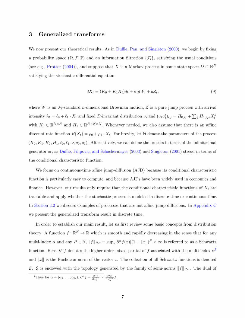
3 Generalized transforms
We now present our theoretical results. As in Duffie, Pan, and Singleton (2000), we begin by fixing
a probability space (Ω,F ,P) and an information filtration Ft, satisfying the usual conditions
(see e.g., Protter (2004)), and suppose that X is a Markov process in some state space D ⊂ RN
satisfying the stochastic differential equation
dXt = (K0 +K1Xt)dt+ σtdWt + dZt, (9)
where W is an Ft-standard n-dimensional Brownian motion, Z is a pure jump process with arrival
intensity λt = `0 + `1 ·Xt and fixed D-invariant distribution ν, and (σtσ′t)i,j = H0,ij +
∑kH1,ijkX
kt
with H0 ∈ RN×N and H1 ∈ RN×N×N . Whenever needed, we also assume that there is an affine
discount rate function R(Xt) = ρ0 + ρ1 ·Xt. For brevity, let Θ denote the parameters of the process
(K0,K1, H0, H1, `0, `1, ν, ρ0, ρ1). Alternatively, we can define the process in terms of the infinitesimal
generator or, as Duffie, Filipovic, and Schachermayer (2003) and Singleton (2001) stress, in terms of
the conditional characteristic function.
We focus on continuous-time affine jump-diffusion (AJD) because its conditional characteristic
function is particularly easy to compute, and because AJDs have been widely used in economics and
finance. However, our results only require that the conditional characteristic functions of Xt are
tractable and apply whether the stochastic process is modeled in discrete-time or continuous-time.
In Section 3.2 we discuss examples of processes that are not affine jump-diffusions. In Appendix C
we present the generalized transform result in discrete time.
In order to establish our main result, let us first review some basic concepts from distribution
theory. A function f : RN → R which is smooth and rapidly decreasing in the sense that for any
multi-index α and any P ∈ N, ‖f‖P,α ≡ supx|∂αf(x)|(1 + ‖x‖)P <∞ is referred to as a Schwartz
function. Here, ∂αf denotes the higher-order mixed partial of f associated with the multi-index α7
and ‖x‖ is the Euclidean norm of the vector x. The collection of all Schwartz functions is denoted
S. S is endowed with the topology generated by the family of semi-norms ‖f‖P,α. The dual of
7Thus for α = (α1, . . . , αN ), ∂αf = ∂α1
∂xα11
· · · ∂αN
∂xαNN
f .
7

S, denoted S∗ and also called the set of tempered distributions, is the set of continuous linear
functionals on S. Any continuous function g which has at most polynomial growth in the sense that
|g(x)| < ‖x‖p for some p and x large enough is seen to be a tempered distribution through the map
f 7→ 〈g, f〉, where we use the inner-product notation
〈g, f〉 =
∫RN
g(x)f(x)dx. (10)
As is standard, we maintain the inner product notation even when a tempered distribution g is
does not correspond to a function as in (10). For example, the δ-function is a tempered distribution
given by 〈δ, f〉 = f(0) which does not arrive from a function.8
For our considerations, the key property is that the set of tempered distributions is suitable
for Fourier analysis. For any Schwartz function f , the Fourier transform of f is another Schwartz
function, denoted f , and is defined by
f(s) =
∫RN
e−is·xf(x)dx. (11)
The Fourier transform can be inverted through the relation
f(x) =1
(2π)N
∫RN
eix·sf(s)ds, (12)
which holds pointwise for any Schwartz function. The Fourier transform is extended to apply to
tempered distributions through the definition 〈g, f〉 = 〈g, f〉. This extension is useful because many
functions define tempered distributions (through (10)), but do not have Fourier transform in the
sense of (11) because the integral in is not well-defined. An example is the Heaviside function:
f(x) = 10≤x ⇒ f(s) = πδ(s)− i
s, (13)
where integrating against 1/s is to be interpreted as the principal value of the integral. Considering
distributions allows us to consider functions which are not integrable and thus in particular may
8Throughout the paper, we use the notation δ(s) to denote the Dirac delta function, with δx(s) = δ(s− x).
8

not decay at infinity and may not even be bounded.
We now state our main result:
Theorem 1. Suppose that g ∈ S∗ and (Θ, α, β) satisfies Assumption 1 and Assumption 2 in
Appendix A. Then
H (g, α, β) = E0
[exp
(−∫ T
0R(Xu)du
)eα·XT g(β ·XT )
]=
1
2π〈g, ψ(α+ ·βi)〉, (14)
where g ∈ S∗ and ψ(α+ ·βi) denotes the function
s 7→ ψ(α+ sβi) = E0
[e−
∫ T0 R(Xu)due(α+isβ)·XT
]. (15)
The function ψ is the transform given in DPS. Recalling their result,
ψ(α+ isβ) = eA(T ;α+isβ,Θ)+B(T ;α+isβ,Θ)·X0 , (16)
where A,B satisfy the ordinary differential equations (ODEs)
B = K>1 B +1
2B>H1B − ρ1 + `1(φ(B)− 1) B(0) = α+ isβ, (17)
A = K>0 B +1
2B>H0B − ρ0 + `0(φ(B)− 1) A(0) = 0, (18)
where φ(c) = Eν [ec·Z ], the moment-generating function of the jump distribution and (B>H1B)k =∑i,j BiH1,ijkBk. Solving the ODE system (17–18) adds little complication to the transform. The
solution is available in closed form in some cases, and can generally be quickly and accurately
computed using standard numerical methods.
In the special case that g defines a function, we can write the result as
H =1
2π
∫ ∞−∞
g(s)ψ(α+ isβ)ds. (19)
Bakshi and Madan (2000) show that option-like payoffs (affine translations of integrable functions)
9

can be spanned by a continuum of characteristic functions. Theorem 1 above shows that the
characteristic functions span a much larger set of functions which includes all tempered distributions.
Equation (19) makes this spanning explicit for the cases where g defines a function.
In some cases of interest, Assumption 2 for Theorem 1 may be violated. It could be that β ·XT
has heavy tails so that, for example, E[(β ·XT )4] =∞. Another example would be in a pure-jump
process where the density may not be continuous. Depending on the case, our result can often be
extended by limiting arguments or by considering different function spaces (such as Sobolev spaces
for non-smooth densities).
There is some flexibility in the choice of α and g in (14). Notice that
eα·XT g(β ·XT ) = e(α−cβ)·XT g(β ·XT ), (20)
where g(s) = ecsg(s). This property can be useful in the case where g is not integrable but decreases
rapidly as s approaches either positive or negative infinity (e.g., the logit function). In this case,
such a transformation of g makes it possible to apply (19).
3.1 Two Extensions
The result of Theorem 1 can be extended in a number of ways. First, we introduce a class of pl-linear
(polynomial-log-linear) functions:
f (α, γ, p,X) =∑i
piXγieαi·X , (21)
where pi are arbitrary constants, αi are complex vectors9 and γi are arbitrary multi-indices
so that Xγ =∏j X
γij . For example with N = 3 and γ = (1, 2, 1), Xγ = X1
1X22X
13 . The following
proposition extends Theorem 1 to work with any pl-linear functions.
Proposition 1. Suppose that g ∈ S∗, and (Θ, α, β, γ) satisfies Assumption 1’ and Assumption 2’
9Allowing complex eigenvalues allows one to have oscillatory sine and cosine terms.
10

in Appendix B. Then
H (g, α, β, γ) = E0
[exp
(−∫ T
0R(Xu)du
)XγT e
α·XT g(β ·XT )
]=
1
2π〈g, ψ(α+ ·βi; γ)〉, (22)
where g ∈ S∗ and ψ(α+ ·βi; γ) denotes the function
s 7→ ψ(α+ sβi; γ) = E0
[e−
∫ T0 R(Xu)duXγ
T e(α+isβ)·XT
]. (23)
The function ψ is computed by solving the associated ODE in Appendix B.
It is immediate from Proposition 1 that we can now compute expectations of the form
H (f, g, α, β) = E0
[exp
(−∫ T
0R(Xu)du
)f(α, γ, p,XT )g(β ·XT )
]. (24)
The assumption that the function g in the generalized transform be a tempered distribution
might appear restrictive at first sight, since g cannot have exponential growth (see our earlier
discussions of Schwartz functions). However, as Proposition 1 demonstrates, by specifying f and g
appropriately, we can let f “absorb” any exponential and polynomial growth in a moment function,
rendering g admissible to the transform. We will demonstrate this feature in several examples.
The transform in Theorem 1 assumes that g can only depend on X through the linear combination
β ·X. Thus, the marginal impact of Xi on g will be proportional to βi, which might be too restrictive
in some cases. The following proposition relaxes this restriction by considering g(β1 ·X, · · · , βM ·X)
for M ∈ N.
Proposition 2. Suppose that g ∈ S∗M (an M-dimensional tempered distribution), α ∈ RN , b ∈
RM×N and (Θ, α, b) satisfies Assumption 1 and Assumption 2 in Appendix A. Then
H (g, α, b) = E0
[exp
(−∫ T
0R(Xs)ds
)eα·XT g(bXT )
]=
1
(2π)M〈g, ψM (α+ ·bi)〉, (25)
11

where g ∈ S∗ and ψM (α+ ·bi) denotes the function
ψM : CM → C , s 7→ ψM (α+ s>bi) = E0
[e−
∫ T0 r(Xu)due(α+is>b)·XT
]. (26)
It is immediate to extend the transform in Proposition 2 by replacing eα·XT with a pl-linear
function as in Proposition 1.
Fourier transforms of many functions are known in closed form (see for example, Folland (1984)).
Additionally, standard rules allow for differentiation, integration, product, convolution and other
operations to be conducted while maintaining closed form expressions. Even if the function g is
not known in closed form, including those cases where g itself is given as an implicit function,
it is straightforward to compute numerically (a 1-dimensional integral in the case of Theorem 1
or Proposition 1, an M-dimensional integral in Proposition 2). Alternatively, one might consider
approximating g with a function g for which the Fourier transform is known in closed form.
Moreover, a convenient feature of the generalized transform is that the Fourier transform of g
and the solutions to the ODEs in (17–18) need only be computed once for a given set of parameters.
Once computed, the Fourier transforms and the differential equation solutions can be used repeatedly
to compute moments with different initial values of the state variable X0 or horizon T . When
the moment function takes the form of f (α, γ, p,X) g(β ·X) as in Proposition 1, the same Fourier
transforms and differential equation solutions can also be used to compute moments with different
pl-linear function f .
3.2 Beyond Affine Jump Diffusions
The key aspects of Theorem 1 and the two extensions are the ability to compute the transform
given in (15), (23), or (26). These transforms are very tractable for affine jump-diffusions. However,
other stochastic processes can also be suitable for the generalized transform, provided that the
appropriate (modified) conditional characteristic function can be computed.
An important example is the class of Levy processes (see for example, Protter (2004)). Levy
processes allow for both finite and infinite activity jumps, though in some contexts the assumption
12
of independent increments may be restrictive. One example of such a process is the variance gamma
(VG) process studied by Madan, Carr, and Chang (1998). The VG process consists of a time-changed
Brownian motion where the clock follows a gamma process. It is a pure jump process that offers
increased kurtosis for increments relative to a standard Brownian motion, which can be useful in
modeling the fat tails in financial data.
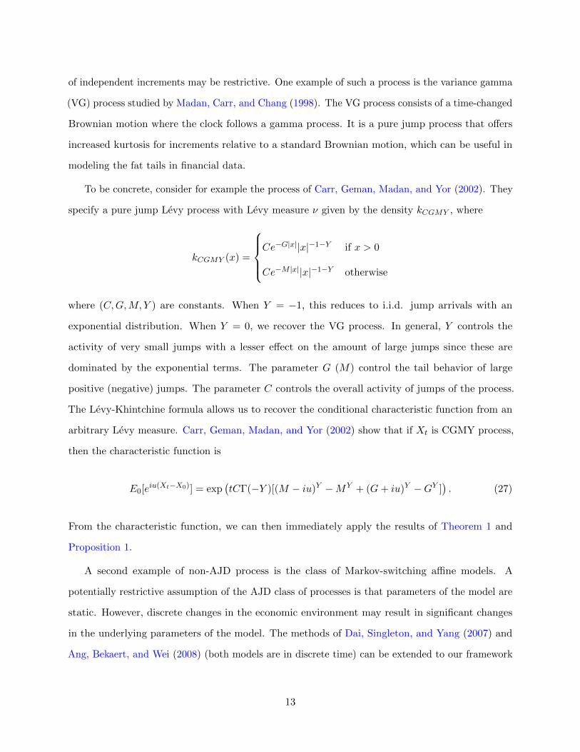
To be concrete, consider for example the process of Carr, Geman, Madan, and Yor (2002). They
specify a pure jump Levy process with Levy measure ν given by the density kCGMY , where
kCGMY (x) =
Ce−G|x||x|−1−Y if x > 0
Ce−M |x||x|−1−Y otherwise
where (C,G,M, Y ) are constants. When Y = −1, this reduces to i.i.d. jump arrivals with an
exponential distribution. When Y = 0, we recover the VG process. In general, Y controls the
activity of very small jumps with a lesser effect on the amount of large jumps since these are
dominated by the exponential terms. The parameter G (M) control the tail behavior of large
positive (negative) jumps. The parameter C controls the overall activity of jumps of the process.
The Levy-Khintchine formula allows us to recover the conditional characteristic function from an
arbitrary Levy measure. Carr, Geman, Madan, and Yor (2002) show that if Xt is CGMY process,
then the characteristic function is
E0[eiu(Xt−X0)] = exp(tCΓ(−Y )[(M − iu)Y −MY + (G+ iu)Y −GY ]
). (27)
From the characteristic function, we can then immediately apply the results of Theorem 1 and
Proposition 1.
A second example of non-AJD process is the class of Markov-switching affine models. A
potentially restrictive assumption of the AJD class of processes is that parameters of the model are
static. However, discrete changes in the economic environment may result in significant changes
in the underlying parameters of the model. The methods of Dai, Singleton, and Yang (2007) and
Ang, Bekaert, and Wei (2008) (both models are in discrete time) can be extended to our framework
13

to incorporate regime shifts for an AJD in the conditional mean, conditional covariance, or the
conditional probability of jumps.
Suppose that there are n possible regimes, denoted by st = 1, · · · , n. The transitions across
different regimes are governed by a continuous-time Markov chain, with the generator matrix
Γ = [γss′ ]. Thus, the probability of the economy moving from regime s to regime s′ over a period ∆t
will be γss′∆t+ o(∆t).10 Now suppose that there is a variable Xt with regime-dependent dynamics:
dXt = (K0(st) +K1Xt)dt+ σtdWt + dZt, (28)
where st is the current regime at time t, W is an Ft-standard n-dimensional Brownian motion, Z is a
pure jump process with arrival intensity λt = `0(st)+`1 ·Xt and fixed D-invariant distribution ν, and
(σtσ′t)i,j = H0,ij(st) +
∑kH1,ijkX
kt with H0(1), · · · , H0(n) ∈ RN×N and H1 ∈ RN×N×N . Now the
dynamics of the state variable are regime dependent with the constant term in the drift, covariance,
and the jump intensity changing across regimes. The (discounted) conditional characteristic function
is given by (15), which will be regime-dependent as well. It follows from (28) that
ψ(α+ isβ, st) = eA(T,st;α+isβ,Θ)+B(T ;α+isβ,Θ)·X0 , (29)
where B is still the solution to the ODE (17) (with no dependence on the regime), and A(t, j) solves
the following regime-dependent system of ODEs:
A(j) = K0(j)TB +1
2BTH0(j)B − ρ0 + `0(j)(φ(B)− 1) +
∑k 6=j
γjk(eA(k)−A(j) − 1) A(0, j) = 0,
(30)
for j = 1, · · · , n. With these modifications, the rest of the generalized transform applies directly.
A third example of processes outside the class of AJDs for which our results apply are the discrete
time autoregressive processes with gamma-distributed shocks. Following the setup of Bekaert and
10We could also assume that the transition probabilities are affine in Xt (which can be easily handled by modifying(17)). Such features of the transition probabilities would be important in the cases where the likelihood of regimeshifts is time-varying.
14

Engstrom (2010) (for simplicity we omit any normally-distributed shocks), suppose Xt follows
Xt+1 = µ+ ΦXt + Σωt+1, (31)
where Σ (n× p) is the conditional volatility matrix for the gamma-distributed shocks, ωt+1 (p× 1),
with ωit+1 ∼ Γ(kit, 1)− kit, and kt = KXt. The conditional characteristic function for Xt+1 is
Et[eiu·Xt+1
]= exp
(iuT (µ+ ΦXt)−
(iuTΣ + ln(1− iuTΣ)
)KXt
)= exp (A(1, u) +B(1, u) ·Xt) , (32)
with
A(1, u) = iuTµ,
B(1, u)T = iuTΦ−(iuTΣ + ln(1− iuTΣ)
)K.
One can then compute the conditional characteristic function for Xt+n (n > 1) through recursion of
formula (32), which renders a pair of difference equations.
The gamma-distributed shocks in the above process provide a convenient way to generate time-
varying skewness and kurtosis. Bekaert and Engstrom (2010) use this process to model aggregate
consumption growth, which helps explain the equity premium and the variance premium. One can
also generalize this autoregressive process in (31) by replacing ωt+1 with other types of shocks that
have tractable characteristic functions.
4 Applications in Contingent Claim Pricing
Having presented the theory of the generalized transform, we now illustrate how it can be applied
to pricing contingent claims. The examples include defaultable bonds with stochastic recovery and
European options with general payoffs.
15

4.1 Recovery risk
Following up on the illustrating example in Section 2, we first discuss the pricing of credit-risky
securities (e.g., defaultable bonds or credit default swaps) with stochastic recovery upon default.
Recovery risk refers to the uncertainty about the recovery rate. In particular, investors will demand
high risk premium if the recovery of these securities are lower in aggregate bad times. For example,
Chen (2010) provides evidence that macro variables such as GDP growth and riskfree rate are
correlated with the aggregate recovery rates and default rates and that such correlations can have
large effects on the pricing of defaultable bonds.
Consider a T year defaultable zero-coupon bond with face value normalized to 1. Following the
literature of reduced-form credit risk models, the default time is assumed to be a stopping time τ
with risk-neutral intensity ht.11 The recovery value at default ϕ is a bounded predictable process
that is adapted to the filtration Ft : t ≥ 0. The instantaneous riskfree rate is rt. Then, the price
of the bond is:
Vt = EQt
[e−
∫ τt rudu1τ≤Tϕτ
]+ EQ
t
[e−
∫ Tt rudu1τ>T
]= EQ
t
[∫ T
te−
∫ st (ru+hu)duhsϕsds+ e−
∫ Tt (ru+hu)du
]. (33)
The second equality follows from the doubly-stochastic assumption and regularity conditions.
Duffie and Singleton (1999) show that under the assumption that the recovery value ϕt is a
proportion 1 − Lt of the market value of the security immediately before default (referred to as
“recovery of market value” (RMV)) and a suitable no-jump condition,12 one can price defaultable
claims with the “default-adjusted discount rate,” rt + λtLt. Moreover, if one directly specifies the
mean-loss rate λtLt and rt as jointly affine under the risk-neutral measure, then the standard results
for affine term structure models can be used to price defaultable bonds.
While analytically appealing, the RMV assumption has some limitations. First, since the default
11To be precise, we fix a probability space (Ω,F ,P) and two filtrations Ft : t ≥ 0, Gt : t ≥ 0. The default timeis a totally inaccessible G-stopping time τ : Ω → (0,+∞]. We assume that under the risk neutral measure Q, τ isdoubly-stochastic driven by the filtration Ft : t ≥ 0. See Duffie (2005) for a survey on the reduced form approachfor modeling credit risk and the doubly-stochastic property.
12The no-jump condition is satisfied here by assuming ϕ is adapted to Ft. See also Duffie, Schroder, and Skiadas(1996) and Collin-Dufresne, Goldstein, and Hugonnier (2004) for discussions on the no-jump condition.
16

intensity ht and the loss rate Lt enter the default-adjusted discount rate symmetrically, we cannot
separately identify the risk-neutral default intensity and recovery rate using information on prices
alone. Second, when pricing bonds of different seniorities from the same issuer, it is more natural to
separately model default intensity (which is the same across different bonds) and recovery rates
(which depend on seniority). Third, data on recovery rates are usually quoted as fraction of face
value instead of market value. For example, Moody’s database of corporate defaults estimates
defaulted debt recovery rates using the ratio of market bid prices (30 days after the date of default)
to par value. The statistical models of recovery rates commonly used by academics and practitioners
are also generally based on par values.
Let Xt be the vector of state variables that determine the riskfree rate, the default intensity,
and the recovery rate. Assume that r(Xt) = ρ0 + ρ1 ·Xt, and h(Xt) = θ0 + θ1 ·Xt. If we model
the recovery value ϕt = g(β · Xt) with a proper function g, then equation (33) clearly fits into
the transform in Proposition 1. This allows us to substantially relax the RMV restriction. In
Appendix E, we calibrate a recovery model that captures the nonlinear relation between recovery
rate and aggregate default intensity in the data. The model shows that ignoring such a relation can
lead to large pricing errors for defaultable securities.
In addition to the logistic model considered in Section 2, we can also model the stochastic
recovery rate using the probit model, the Cauchy model, or the cumulative distribution functions
associated with any other probability distributions.13 Such flexibility in modeling the recovery
rate makes the above framework well suited to connect models of defaultable bond pricing with
commonly used statistical models of recovery rates.
4.2 Option pricing
When pricing European options, we want to compute expectations of the form
EQt
[e−
∫ Tt rsds+α·XT gy(β ·XT )
], (34)
13Bakshi, Madan, and Zhang (2006) study a class of recovery models for which ϕ is exponential affine in the defaultintensity as well as the class of completely monotone functions. They solve for bond prices using the DPS transform.The completely monotone class requires that each order derivative is either always positive or negative.
17

where gy(x) = 1x≤y is nonlinear and non-integrable. For example, for a European put option with
strike K, β ·Xt will be the log stock price, y = logK, and the option price is
Pt = EQt
[e−
∫ Tt rsds+ygy(β ·XT )
]− EQ
t
[e−
∫ Tt rsds+β·XT gy(β ·XT )
]. (35)
The Fourier transform of gy is defined as a distribution:
gy(s) = πδ(s) +ie−isy
s, (36)
where the second term is interpreted as a principal value integral. It follows that
EQt
[e−
∫ Tt rsds+α·XT gy(β ·XT )
]=
∫ ∞−∞
(δ(s)
2− e−isy
2πis
)ψ(α+ isβ)ds
=ψ(α)
2−∫ ∞
0Real
(ψ(α+ isβ)e−isy
πis
)ds. (37)
In the last equation we use the fact that the real part of the integrand is even and the imaginary
part is odd. This replicates the formula given in DPS obtained by Levy-inversion.14
Since the generalized transform only requires the state variable to have a tractable conditional
characteristic function, we have a lot of flexibility in modeling the underlying uncertainty. Our
method also applies to exotic options whose payoffs are more complicated functions of the state
variables (such as the terminal value of the stock), as long as the payoff can be written in the form
of a product of a pl-linear function and a tempered distribution.
Bakshi and Madan (2000) (henceforth BM) also provide a more general method than DPS for
pricing options. It allows for payoffs of the form (H(XT )−K)+, where X is a univariate stochastic
process with known conditional characteristic function under the risk-neutral measure, H is a
positive and entire function,15 and K is a fixed strike price. They propose a power series expansion
of H, the expectations of which can then be computed through differentiation of the conditional
14In DPS, they arrive at this equation by effectively computing the forward density by Fourier transform (a1-dimensional integral) and then integrating over the payoff region (now a 2-dimensional integral). In this case, Fubiniand limiting arguments allow this 2-dimensional integral to be reduced to a 1-dimensional integral as in the standardLevy inversion formula (without a forward measure).
15An entire function is one that is analytic at all finite points on the complex plane.
18

characteristic functions. Their method applies to non-affine processes as well (see Section 3.2).
Our method differs from BM in several aspects. First, the power series expansion approach in
BM requires that H be infinitely differentiable and that the power series converges to H(X) for all
X. However, there can be cases where the payoff function has many kinks or is not entire (simple
examples include ln(X) and√X). Second, in those cases where the Fourier transform g is known,
our method requires only one 1-dimensional integration, whereas the method of BM requires one
1-dimensional integration and one infinite sum. Third, we extend BM’s result on spanning of option
payoff with characteristic functions. In BM, the set of payoff functions H that can be spanned
by characteristic functions is an affine translation of an L1 function (see BM Theorem 1).16 We
relax the growth condition on the underlying payoff; the dual space S∗ is quite large and contains
Lp for any p, as well as functions not in Lp for any p. Finally, our theory extends the analysis to
multivariate settings.
To illustrate some of these differences, consider the payoff of the form H(X) = Xα for a positive
non-integer α. In this case H is not entire (for any choice of X0, the power series converges to H(X)
only for 0 < X < 2X0).17 Nor is it an affine translation of an L1 function. However, we can still
use the fact that H represents a tempered distribution to write
g(s) = (−is)−1−αΓinc(−α− 1,−is), (38)
where Γinc(·, ·) denotes the incomplete Γ function and s−1−α is interpreted in the sense of a
homogeneous tempered distribution.
5 Applications in Economic Modeling
Affine general equilibrium models are attractive due to their tractability. This class of models
starts with state variables Xt that are affine and develop (either exogenously or endogenously) the
16A function H is of class Lp if(∫|H(x)|pdx
)1/p<∞.
17In practice, one may still compute option prices through the Taylor expansion of an non-entire payoff functionwith reasonable accuracy for special choices of X0 and the order of Taylor expansion, although it is not obvious whatchoices would be optimal ex ante.
19

stochastic discount factor Mt as an exponential affine function of Xt:
Mt = m(t,Xt) = exp(−ρt− a ·Xt). (39)
For example, in an endowment economy, the SDF is the marginal utility of the representative agent,
which depends on the log endowment and potentially other state variables that are jointly affine.18
Under these assumptions, it is easy to show that the riskfree rate rt is affine in Xt, and X is still
affine under the risk-neutral probability measure Q. As a result, the value a security with payoff
YT = y(XT ) at time T can be computed as
Pt = EQt
[e−
∫ Tt ruduy(XT )
], (40)
which can be solved analytically using the DPS transform provided that y(X) is a pl-linear function
of X, or using the generalized transform if y(X) can be decomposed into the product of a pl-linear
function f(X) and a function with a Fourier transform g(β ·X) as in Proposition 1.
However, the benefit of the generalized transform is not limited to dealing with nonlinear payoffs.
Consider the case where m(t,X) is not exponential affine (but still strictly positive). The value of
the security above can also be computed as
Pt =1
m(t,Xt)Et [m(T,XT )y(XT )] . (41)
This expectation can be computed using the generalized transform provided that m(T,X)y(X) =
f(X)g(β ·X) as in Proposition 1. Then, the riskfree rate rt is no longer required to be affine in Xt,
and X is generally no longer an affine process under Q.
To see this, suppose m(t,Xt) = e∫ t0 R(Xs)dsg(β ·Xt), where R(Xt) = ρ0 + ρ1 ·Xt, and X follows
an affine diffusion (it is also easy to add jumps). Then, the Ito’s lemma implies that the riskfree
18Examples include Bakshi and Chen (1997), Bekaert and Grenadier (2002), Mamaysky (2002), Longstaff andPiazzesi (2004), among others.
20

rate is
rt = −(ρ0 + ρ1 ·Xt)−g′(β ·Xt)
g(β ·Xt)βT (K0 +K1Xt)−
1
2
g′′(β ·Xt)
g(β ·Xt)tr(ββTσtσ
′t),
and under the risk-neutral measure X follows
dXt =
(K0 +K1Xt +
g′(β ·Xt)
g(β ·Xt)σtσ′tβ
)dt+ σtdW
Qt .
Both the risk free rate and the conditional mean of Xt under Q are nonlinear, making it unsuitable
to do valuation directly under Q. Instead, valuation under P using (40) can still be very tractable.
Again, as discussed in Section 3.2, X does not need to be an affine jump-diffusion. All that is
required is that its conditional characteristic function is tractable.
Next, we discuss some specific examples where non-exponential affine stochastic discount factors
arise in realistic settings.
5.1 An Affine Model of External Habit
The external habit model of Campbell and Cochrane (1999) is a workhorse in asset pricing that
helps generate a high and time-varying equity premium even though consumption growth is i.i.d.
and has low volatility. Solving this model as well as estimation and forecasting can be challenging
due to the complicated dynamics of the external habit process. In this example, we construct a
habit process based on affine state variables that captures the desired features of the habit model.
Our construction is based on the continuous-time version of the external habit model in Santos
and Veronesi (2010). In an endowment economy, the representative agent’s utility over consumption
stream Ct is
E
[∫ ∞0
e−ρt(Ct −Ht)
1−γ
1− γ dt
], (42)
where Ht is the habit level that is positive and strictly below Ct. The log aggregate endowment
21
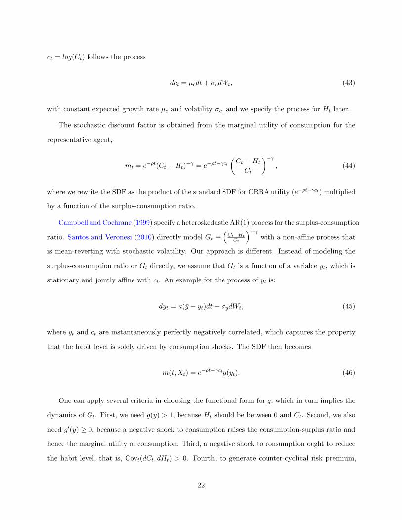
ct = log(Ct) follows the process
dct = µcdt+ σcdWt, (43)
with constant expected growth rate µc and volatility σc, and we specify the process for Ht later.
The stochastic discount factor is obtained from the marginal utility of consumption for the
representative agent,
mt = e−ρt(Ct −Ht)−γ = e−ρt−γct
(Ct −Ht
Ct
)−γ, (44)
where we rewrite the SDF as the product of the standard SDF for CRRA utility (e−ρt−γct) multiplied
by a function of the surplus-consumption ratio.
Campbell and Cochrane (1999) specify a heteroskedastic AR(1) process for the surplus-consumption
ratio. Santos and Veronesi (2010) directly model Gt ≡(Ct−HtCt
)−γwith a non-affine process that
is mean-reverting with stochastic volatility. Our approach is different. Instead of modeling the
surplus-consumption ratio or Gt directly, we assume that Gt is a function of a variable yt, which is
stationary and jointly affine with ct. An example for the process of yt is:
dyt = κ(y − yt)dt− σydWt, (45)
where yt and ct are instantaneously perfectly negatively correlated, which captures the property
that the habit level is solely driven by consumption shocks. The SDF then becomes
m(t,Xt) = e−ρt−γctg(yt). (46)
One can apply several criteria in choosing the functional form for g, which in turn implies the
dynamics of Gt. First, we need g(y) > 1, because Ht should be between 0 and Ct. Second, we also
need g′(y) ≥ 0, because a negative shock to consumption raises the consumption-surplus ratio and
hence the marginal utility of consumption. Third, a negative shock to consumption ought to reduce
the habit level, that is, Covt(dCt, dHt) > 0. Fourth, to generate counter-cyclical risk premium,
22

we would like negative shocks to consumption to raise the conditional Sharpe ratio of the market
portfolio (the price of risk for consumption shocks):
SR(yt) = γσc +g′(yt)
g(yt)σy. (47)
Thus, we need ddySR(y) = d
dy log(g(y)) ≥ 0.
Finding such a function g is straightforward, and it is clear that it cannot be exponential-affine
in y.19 Suppose the desired range of Sharpe ratio is between γσc and γσc +α for some α > 0. Then,
we can assume
g′(y)
g(y)=
α
σyF (y), (48)
where F is any monotone non-decreasing function with
limy→−∞
F (y) = 0, limy→+∞
F (y) = 1.
For example, F can be the cumulative distribution function of any real univariate random variable.
Thus, we have a lot of flexibility in choosing the desired shape of F , which in turn decides the
distribution of the conditional Sharpe ratio.
It follows that
g(y) = exp
(b+
α
σy
∫ y
−∞F (t)dt
), (49)
which satisfies the criteria we discussed earlier for g provided the constant b is sufficiently large.20
The SDF in (46) fits the moment function in Theorem 1 (with an appropriate choice of factorization
as in (20)). This example highlights the power of the generalized transform: rather than specifying
a complicated process for g directly, we can utilize the flexibility in choosing g(y) for some tractable
process y (such as an affine process).
19In the special case where m(t,Xt) follows the exponential-affine form in (39), one can show that if consumptionshocks are i.i.d. and Xt is affine, the price of consumption shock has to be constant.
20To satisfy the condition Covt(dCt, dHt) > 0, it suffices to have b > γ ln(
1 + αγσc
).
23
5.2 Heterogeneous agents economy
The generalized transform can also be used to solve models with heterogeneous agents. The
heterogeneity could be about preferences or beliefs. Earlier work include Dumas (1989) and Wang
(1996), among others. The stochastic discount factors in the general form of these models will be
implicit functions of stochastic state variables. However, even in these general cases, the generalized
transform can still be applied.
For illustration, we assume that there is a single risky asset in an endowment economy. Two
infinitely-lived agents A and B have time-separable preferences over consumption stream ct:
Ui(c) = E0
[∫ ∞0
ui (ct, t) dt
], i = A,B (50)
We model the dividend process D from the risky asset as part of a general affine jump-diffusion.
Specifically, suppose log dividend dt = ι1 ·Xt, where Xt is a vector that follows the process (9). This
model can easily capture features such as predictability in dividend growth, stochastic volatility, or
time-varying probability of jumps. For example, to get predictability of dividend growth, we can
assume
ddt = gtdt+ σddWdt (51a)
dgt = κg (g − gt) dt+ σgdWgt (51b)
where gt is the expected growth rate of dividends, which follows an Ornstein-Uhlenbeck process
with long run mean g. The state variable is then given by Xt = [dt gt]′, and it is straightforward to
verify that X is affine with coefficients implied by the dynamics of dt and gt. Finally, as discussed
in Section 3.2, other non-AJD processes with tractable conditional characteristic functions can be
used for Xt as well.
Assuming markets are complete, we can first solve for the optimal allocations through the social
planner’s problem
maxCA,CB
E0
[∫ ∞0uA (CA,t, t) + λuB (CB,t, t) dt
], (52)
24
which has constant relative Pareto weight λ and is subject to the market clearing condition
CA,t + CB,t = Ct. For concreteness, consider the case where the agents have power utility and
differ only in their relative risk aversion, ui (c, t) = e−ρtc1−γi/(1− γi), with γA 6= γB. The optimal
allocations can be solved through the planner’s first order conditions and the market clearing
condition. Except for a few special cases,21 agent A’s equilibrium consumption is an implicit
function of aggregate endowment
CA,t = f
(D
1− γBγA
t
)Dt. (53)
Then, the unique stochastic discount factor in this economy is given by
ξt = e−ρtf
(D
1− γBγA
t
)−γAD−γAt = e−ρtg(dt)e
−γAdt . (54)
where g is an implicit function that is smooth and bounded. The generalized transform can now be
applied when we use the discount factor to price claims. For example, the price of a zero coupon
bond that pays one unit of consumption at time T is
B(t, T ) = Et
[ξTξt
]=
e−ρ(T−t)
f(dt)e−γAdtEt[e−γAι1·XT g(ι1 ·XT )
], (55)
where Theorem 1 can be applied to evaluate the expectation in (55). In case where there is an
explicit formula for g, the transform may be known in closed form. However, even when g does
not have a closed form solution, one will only need to compute g numerically once: this single
calculation can then be used for the valuation of a variety of securities and need not be re-computed
for different horizons.
Besides heterogeneous preferences, the above model framework can also be used to study
heterogeneity in beliefs across agents, provided that the beliefs of the agents satisfy the “affine-
disagreement framework” (Chen, Joslin, and Tran (AER 2010)).22 We can also extend the model to
N > 2 agents, which will only change the functional form of g for the SDF in (54) (the transform
21Wang (1996) shows that the model can be solved in closed form when γA = nγB where n = 2, 3, 4.22See Appendix D for more discussion on affine differences in beliefs. Bhamra and Uppal (2010) provide a recent
treatment of heterogeneous preferences and beliefs when the underlying uncertainties are i.i.d.
25

remains one-dimensional), or to a model of international finance with multiple goods and multiple
countries as in Pavlova and Rigobon (2007).
5.3 Multiple goods economy
Our next example is to solve for the equilibrium in an endowment economy with two assets. Several
recent papers have studied the general equilibrium effects of multiple sources of consumption in an
endowment economy. See Santos and Veronesi (2006) (analytical result for a model with financial
asset and labor income that satisfy special co-integration restrictions), Piazzesi, Schneider, and
Tuzel (2007) (numerical solution for a model with housing and non-housing consumption), Cochrane,
Longstaff, and Santa-Clara (2008) (analytical result for a model with two i.i.d. trees and log utility),
and Martin (2008) (analytical results for N i.i.d. trees and power utility).
There are two assets (or two types of consumption goods) in the economy, both in unit supply,
with dividend streams D1,tdt and D2,tdt. As in the previous section, we assume that the log
dividends d1,t = logD1,t and d2,t = logD2,t are part of a vector Xt (d1,t = ι1 ·Xt, d2,t = ι2 ·Xt),
which follows an affine jump-diffusion (9). Again, this model can allow for time variation in the
expected dividend growth rates, stochastic volatility, and time variation in the probabilities of jumps.
Co-integration restriction can also be imposed.
There is an infinitely-lived representative investor with CRRA utility over aggregate consumption:
U(c) = E0
[∫ ∞0
e−ρtC1−γt − 1
1− γ dt
], (56)
where aggregate consumption is a CES aggregator of the two goods D1,t and D2,t,
Ct =(D
(ε−1)/ε1,t + ωD
(ε−1)/ε2,t
)ε/(ε−1). (57)
The parameter ε is the elasticity of intratemporal substitution between the two goods, and ω
determines the relative importance of the two goods.
We can recover the continuous time version of Piazzesi, Schneider, and Tuzel (2007) when we
interpret D1,t and D2,t as housing and nonhousing consumption, respectively, and assume that
26
the growth rate of nonhousing consumption is i.i.d., the log ratio of the two dividends follows a
square-root process. In the case ε→∞ and ω = 1, the two goods become perfect substitutes, so
that Ct = D1,t +D2,t. This is the case considered by Cochrane, Longstaff, and Santa-Clara (2008)
and Martin (2008), both of which assume i.i.d. dividend growth.
In equilibrium, the unique stochastic discount factor ξt = e−ρtC−γt . Under the standard regularity
conditions, the price of asset i (i = 1, 2), Pi,t, is then given by:
Pi,t = Et
[∫ ∞0
ξt+uξt
Di,t+udu
]
=(D
(ε−1)/ε1,t + ωD
(ε−1)/ε2,t
)γε/(ε−1)∫ ∞
0e−ρuEt
Di,t+u(D
(ε−1)/ε1,t+u + ωD
(ε−1)/ε2,t+u
)γε/(ε−1)
du. (58)
The main challenge of computing the stock price comes from the stochastic discount factor,
which is non-pl-linear in the state variable Xt. To map the expectation in (58) into the generalized
transform, we rewrite the expectation inside the integral of (58) as:
Et
D1,s(D
(ε−1)/ε1,s + ωD
(ε−1)/ε2,s
)γε/(ε−1)
= Et
e(1−γ/2)d1,s−γ/2d2,s(2 cosh
(ε−1ε
d1,s−d2,s2
))γ
= Et [f (α ·Xs) g (β ·Xs)] , (59)
where
f (x) = ex
g (x) =1
(2 cosh(x))γ
and
α =(
1− γ
2
)ι1 −
γ
2ι2, β =
ε− 1
2ε(ι1 − ι2).
Since X is affine and g ∈ S∗, Theorem 1 readily applies to (59). When the increments of X are
i.i.d., the conditional characteristic function for X is known explicitly, which Martin (2008) uses to
compute (59) following a Fourier transform for g. In this i.i.d. increment case, the process for X
27

can be generalized to any Levy process as in Section 3.2.
Several observations are in order. First, when we introduce additional state variables to X within
the affine framework, due to the time-separable utility function, these additional state variables do
not directly enter into the pricing equation (58). Hence, adding these new state variables do not
increase the dimension of the Fourier transform. Second, we can generalize the utility function, e.g.,
by making aggregate consumption Ct a CES aggregator of D1,t and D2,t, as in Piazzesi, Schneider,
and Tuzel (2007), where the two trees are interpreted as nonhousing consumption and housing
services. It is also convenient to add preference shocks that are pl-linear in the state variables.
Third, the model can allow for multiple trees using the multi-dimensional version of the generalized
transform in Proposition 2. Finally, although our method computes stock values as an average of
exponential affine functions of the state, when pricing options on stocks, the exercise regions will
typically be a non-linear function of all covariates. In this case, we can proceed as in Singleton and
Umantsev (2002) to approximate the option value by linearizing the exercise region and using the
closed form valuation of the payoff.
5.4 A concrete example: time-varying labor income risk
In this section, we study a general equilibrium model with time-varying labor income risk. This
model not only serves a concrete example of applying the generalized transform method for economic
analysis, but also draws a number of new insights on how the time-varying covariance between labor
income and dividends affects asset pricing.
In consumption-based asset pricing models, the covariance between shocks to consumption and
cash flows of an asset is often a key determinant of the risk premium for the asset. As this covariance
fluctuates over time, so will the implied risk premium. Santos and Veronesi (2006) (hereafter SV)
point out a natural source of such time variation in the covariances via a composition effect : as
the share of labor income in total consumption varies over time, so will the covariances between
consumption and dividends, which in turn generates time-varying equity premium. Intuitively,
higher labor income relative to dividends tends to make investors less sensitive to fluctuations in
dividend income. Santos and Veronesi illustrate this point in a model with stationary labor share
28

1945 1950 1955 1960 1965 1970 1975 1980 1985 1990−0.5
0
0.5
1
1.5
2
r 4y
1945 1950 1955 1960 1965 1970 1975 1980 1985 19900.7
0.75
0.8
0.85
0.9
0.95
L/C
A. 1947−1990
1990 1992 1994 1996 1998 2000 2002 2004 2006 2008 2010 2012−2
−1
0
1
2
r 4y
1990 1992 1994 1996 1998 2000 2002 2004 2006 2008 2010 20120.76
0.78
0.8
0.82
0.84
L/C
B. 1991−2010
Figure 1: Long-term returns and labor share pre and post-1990. Data is quarterly and the
sample period is 1947Q1 to 2010Q2. L/C is the share of labor income to consumption. r4y is the lagged
four-year cumulative returns of the market portfolio. We use per-capita consumption (nondurables and
services) from the BEA and labor income series constructed following Lettau and Ludvigson (2001a).
and multiple financial assets, which provides very convenient closed-form solutions for asset prices.
Following SV, we plot in Figure 1 the share of labor income and lagged four-year cumulative
returns of the CRSP value-weighted market index. The labor share is defined as the ratio of labor
income to consumption. Consistent with the findings of SV, the labor share and lagged market
return in Panel A of Figure 1 are negatively correlated, with an average correlation of −0.35.
However, in the post-1990 period, the two series become positively correlated, which is opposite
of the composition effect.23 These results suggest that other covariates may be playing a role in
determining the relationship between the labor share and the equity premium (see also Duffee (2005)
and Kozhanov (2009) for related findings).
One example of such covariates is consumption volatility. Lettau, Ludvigson, and Wachter
23In fact, to some extent this effect is already documented in Santos and Veronesi (2006) (Table 2), where theyshow that the predictive power of the labor share is stronger in the sample 1948-1994 than in 1948-2001.
29

(2008) argue that declining macroeconomic volatility since the 1980s has played a key role in the
decline of the equity premium and of dividend yields.24 In Figure 2, we plot the volatility of
consumption growth for non-overlapping 5-year periods using quarterly data from 1952 to 2010.
In addition, we also plot the correlation between labor income and dividends during the same
periods. Interestingly, the correlation between labor income and dividends shows a similar pattern
as volatility. It ranges from the peak of 0.1 in early 1980s to the low of −0.9 in the late 1990s, and it
also tends to rise when consumption volatility rises. Like changes in consumption volatility, changes
in the correlation between labor income and dividends could also affect the equity premium. All else
equal, consumption volatility should indeed rise with the correlation between its two components.
However, consumption volatility could also change independently of the correlation, e.g., through
time-varying share of labor income in consumption, or variations in the volatilities of labor income
and dividends.25
Motivated by these findings, we propose a simple model that captures these interesting dynamics
of the conditional moments of labor income, dividends and consumption. The model is a special
case of the two-asset model discussed in Section 5.3, with dividends from the two assets interpreted
as financial income (dividends) and labor income. We extend the models of Cochrane, Longstaff,
and Santa-Clara (2008) and Martin (2008) in two important dimensions: (1) we add a volatility
factor, which simultaneously drives the conditional volatilities of labor income and dividends, as
well as the correlation between the two; (2) we impose cointegration between labor income and
dividends to ensure the long run stationarity of labor share. Our model also differs from SV in that
labor share and the correlation between labor income and dividends can move independently. The
affine family of processes allow us to achieve all of the objectives as follows.
Let log dividends and log labor income be dt and `t, and let Vt be a volatility factor. Suppose
24They estimate a structural break occurred in consumption volatility in 1991, which motivates our choice of thetwo subsamples in Figure 1.
25Different economic mechanisms may have lead to the decline in consumption volatility and the decline in correlationbetween labor income and dividends. A number of authors have attributed the great moderation to transparency inmonetary policy. On the other hand, Piketty and Saez (2003) demonstrate that in the mid-1980s, income inequalitybegan to rise. This “Great Divergence” is consistent with a increasingly negative correlation between labor incomeand dividends and may have been linked to structural changes associated with legal changes and the declining role oflabor unions (see, for example, Card (2001)).
30

1950 1960 1970 1980 1990 2000 20100.005
0.01
0.015
0.02
σ c
volatilitycorrelation
1950 1960 1970 1980 1990 2000 2010−1
−0.5
0
0.5
corr(ℓ
t,d t)
Figure 2: Consumption volatility and correlation between labor income and dividends.This figure plots the (annualized) standard deviation of aggregate consumption growth and the correlation
between the growth rates of labor income and dividends in 5-year windows. The data are quarterly from
1952Q1 to 2010Q2. At the end of each series we add the estimate for the most recent 5 years.
Xt = (dt, `t, Vt)′ follows an affine process
dXt = µtdt+ σtdWt. (60)
We assume that the conditional drift µt is given by
µt =
g − a κs(s− (`t − dt))
g + (1− a)κs(s− (`t − dt))
κV (V − Vt)
. (61)
This formulation gives the same average growth rate of g for dividends and labor income. The
second term in the growth rates of dividends and labor income allows for the shares of labor income
and dividends to be stationary. To see this, consider the dynamics of the log labor income-dividend
ratio st = `t − dt. Equation (61) implies that the drift of st will be κs(s − st), with s being the
long-run average of the log labor income-dividends ratio, and κs ≥ 0 the speed of mean reversion.
Thus, when the share of labor income relative to dividends is high, the expected growth rate of
31

dividends will be higher than that of labor income, which causes st to revert to its long-run mean.
The opposite is true when the labor share is low. The parameter a gives us additional flexibility
in specifying the degree of time variation in the growth rates of dividends and labor income. For
example, a = 1 implies that the expected labor income growth is constant over time. Equation (61)
also implies that the volatility factor Vt is stationary, with long-run mean V and speed of mean
reversion κV .
The conditional covariance of the factors is given by
σtσ′t = Σ0 + Σ1Vt, (62)
where Σ0 and Σ1 can be any positive semi-definite matrices with the the restriction Σ0,33 = 0 so that
the volatility factor always remains positive. According to the terminology of Dai and Singleton
(2000), this is an A1(3) model of dividends and labor income. As Vt increases, the volatilities of
dividends and labor income will increase. Moreover, the instantaneous correlation between dividends
and labor income, ρt, also varies with the volatility factor Vt:
ρt =Σ0(1, 2) + Σ1(1, 2)Vt√
Σ0(1, 1) + Σ1(1, 1)Vt√
Σ0(2, 2) + Σ1(2, 2)Vt. (63)
The structure of a single volatility factor implies that the correlation and volatilities have to
move in lock steps. While this feature is clearly restrictive, it allows us to capture the comovement
between consumption volatility and correlation demonstrated in Figure 2, and it helps keep the
number of state variables small. It is possible to substantially relax the covariance structure using the
Wishart process, which allows for fully stochastic covariance between labor income and dividends.
Section 5.3 already explains how to price the stock and human capital using the generalized
transform. To compute the expected excess returns and volatilities of the stock and human capital,
we can consider them as portfolios of zero-coupon equities, each of which with one “dividend”
payment Dt or Lt. The risk premium of the stock or human capital is then the value-weighted
average of the risk premium for these zero-coupon equities. In general, the instantaneous expected
excess return for any asset is determined by its exposure to the primitive shocks in the state variable
32
Xt and the risk prices associated with these shocks, which in turn are determined by their covariances
with the stochastic discount factor Mt. Thus, by Ito’s Lemma, the expected excess return for any
asset with price Pt = P (Xt, t) is given by
Et[Re] = (∇X logMt)
′ σtσ′t (∇X logPt) , (64)
where σtσ′t, the time t covariance of the factors, is given in (62). Here (∇X logMt)
′ σt in (64) gives
the price of risk for all the shocks in Xt, while (∇X logPt)′ σt gives the exposure that the asset
has to these shocks. With power utility, only those shocks that directly affect consumption will be
priced in the equilibrium. The assumption that the volatility factor Vt is independent of dividends
and labor income then implies that shocks to dividends and labor income are the only ones with
nonzero risk prices in our model. Finally, since the covariance among the factors is time-varying in
our model, both the prices of risk and risk exposures can change over time.
Next, we examine the risk premium on financial wealth and human capital. The risk premium
for financial wealth depends on its exposure to both dividend and labor income shocks. First, the
financial wealth claim is directly exposed to dividend shocks via its cash flows (dividends). Second,
via the discount factor, it is exposed to both dividend and labor income shocks.26 Both mechanisms
will have an effect on the risk premium. For example, positive shocks to labor income will decrease
the premium demanded for dividends, increase the risk-free rate (as a higher share of the less
volatile labor income tends to smooth consumption, reducing the precautionary savings motive),
and increase expected future dividends due to the mean reversion in (61) (with a > 0). The solution
of our model allows us to incorporate all of these mechanisms to determine the risk premium for
the dividend claim.
Figure 3 plots the conditional risk premium on financial wealth and human capital as functions
of the labor share and correlation. We leave the details of model calibration to Appendix F. The
parameters are summarized in Table 2. We focus on the region that is more relevant based on
the stationary distributions of the two variables. Both the labor share and stochastic covariance
are important contributor to the risk premium. When volatilities and correlations are high, the
26The value of the dividends tree will also be sensitive to covariance shocks (Vt). However, these shocks are notpriced in our model by the assumption that they are not correlated with consumption.
33

0.6
0.7
0.8
0.9
−0.6
−0.4
−0.2
0
0.02
0.04
0.06
0.08
Lt/Ct
A. Premium on financial wealth
ρt 0.6
0.7
0.8
0.9
−0.6
−0.4
−0.2
0.01
0.02
0.03
0.04
Lt/Ct
B. Premium on human capital
ρt
Figure 3: Conditional risk premium on financial wealth and human capital. The left panel
plots the conditional risk premium on the stock (financial wealth), and the right panel plots the conditional
risk premium on human capital as function of labor share Lt/Ct and correlation ρt.
model generates significant composition effect: When the correlation ρt = −0.1, the conditional risk
premium on financial wealth falls from 6.6% to 1.8% as labor share rises from 0.6 to 0.9. However,
when ρt = −0.8, the risk premium essentially remains at 0 for the same rise in labor share. What’s
more, consistent with the prediction on the price of dividend risk, the risk premium on financial
wealth is more sensitive to changes in volatility and correlation when labor share is low.
Why is the risk premium changing so little with the labor share when volatilities are low? First,
as labor share rises, the composition effect tends to drive down the risk premium per unit of dividend
risk, but this effect weakens as the volatility falls. At the same time, the price-dividend ratio (P/D)
is rising (due to both lower risk free rate and higher expected dividend growth) and becoming
more sensitive to changes in labor share, hence also more sensitive to labor income and dividend
shocks (with opposite signs). Since the price of labor income risk is rising with higher labor share
while the price of dividend risk is decreasing, the net effect via the price-dividend ratio tends to be
offsetting the composition effect for sufficiently high labor share. Moreover, when volatility falls,
the rise in the price of labor income risk accelerates, which strengthens the P/D effect. Under our
parameterizations, when volatilities are sufficiently low, the two effects essentially cancel each other.
34

As for the risk premium on human capital, the composition effect is stronger when the correlation
is low, which is again consistent with our earlier analysis of the price of labor income risk. For
example, when ρt = −0.8, the premium on human capital rises from 0 to 1.8% as labor share rises
from 0.6 to 0.9. As the correlation rises, the premium flattens and eventually becomes U-shaped in
labor share.
Through the lens of our model, we can also analyze the comovement between the risk premium
on financial wealth and human wealth.27 Cash flows from the claim on financial and human wealth
are negatively correlated most of the time in our model. However, both positive and negative
correlation between the risk premium on financial and human wealth can occur. The risk premium
on financial wealth and human wealth will be negatively correlated when the composition effect is
the main driver of variations in risk premium over time. However, when variations in the volatilities
and correlation become the main driver of variations in risk premium, the two risk premiums will
become positively correlated.
6 Conclusion
We extend the transform analysis in Duffie, Pan, and Singleton (2000) to compute a general class of
nonlinear moments for affine jump-diffusions. Through a Fourier decomposition of the nonlinear
moments, we can directly utilize the properties of the conditional characteristic functions for affine
processes and compute the moments analytically. By not resorting to an intermediate computation
of the (forward) density, this method greatly reduces the dimensionality of such problems, allowing
for tractability in a wide range of economic applications.
We demonstrate the power of this method with examples from several areas, including defaultable
bond pricing, option pricing, and equilibrium asset pricing models with heterogeneous agents or
multiple goods. Underlying all of these examples are the rich dynamics provided by affine processes,
allowing for time-varying conditional means and variances as well as jumps occurring with stochastic
intensity. Finally, we apply the generalized transform method in a general equilibrium model of
27Previous studies have different findings when measuring the sign of this comovement in the data. For example,see Hansen, Heaton, Lee, and Roussanov (2007) and Lustig and Van Nieuwerburgh (2008).
35

time-varying labor income risk. The model not only helps explain the changing predictive power of
labor share with declining volatility, but also shows that the risk premium on financial wealth and
human capital can be positively or negatively correlated, depending on whether variations in labor
share or covariances are the main driver of risk premium.
36

References
Abramowitz, M., and I. A. Stegun, 1964, Handbook of Mathematical Functions with Formulas,
Graphs, and Mathematical Tables, Dover, New York, ninth dover printing, tenth gpo printing edn.
Altman, E. I., B. Brady, A. Resti, and A. Sironi, 2005, “The Link between Default and Recovery
Rates: Theory, Empirical Evidence, and Implications,” Journal of Business, 78, 2203–2228.
Ang, A., G. Bekaert, and M. Wei, 2008, “The Term Structure of Real Rates and Expected Inflation,”
Journal of Finance, 63, 797–849.
Bakshi, G., C. Cao, and Z. Chen, 1997, “Empirical Performance of Alternative Option Pricing
Models,” Journal of Finance, 52, 2003–49.
Bakshi, G., and D. Madan, 2000, “Spanning and derivative-security valuation,” Journal of Financial
Economics, 55, 205–238.
Bakshi, G., D. Madan, and F. Zhang, 2006, “Understanding the Role of Recovery in Default Risk
Models: Empirical Comparisons and Implied Recovery Rates,” Working paper.
Bakshi, G. S., and Z. Chen, 1997, “An alternative valuation model for contingent claims,” Journal
of Financial Economics, 44, 123–165.
Basak, S., 2005, “Asset Prices with Heterogenous Beliefs,” Journal of Banking & Finance, 29,
28492881.
Bates, D. S., 1996, “Jumps and Stochastic Volatility: Exchange Rate Processes Implicit in Deutsche
Mark Options,” Review of Financial Studies,, 9, 69–107.
Bekaert, G., and E. Engstrom, 2010, “Asset Return Dynamics under Bad Environment-Good
Environment Fundamentals,” Working Paper.
Bekaert, G., and S. Grenadier, 2002, “Stock and Bond Pricing in an Affine Equilibrium,” Working
Paper.
Bhamra, H. S., and R. Uppal, 2010, “Asset Prices with Heterogeneity in Preferences and Beliefs,”
Working Paper.
Buraschi, A., F. Trojani, and A. Vedolin, 2010, “Economic Uncertainty, Disagreement, and Credit
Markets,” Working Paper, Imperial College Business School.
Campbell, J. Y., and J. H. Cochrane, 1999, “By Force of Habit: A Consumption Based Explanation
of Aggregate Stock Market Behavior,” Journal of Political Economy, 107, 205–251.
Card, D. E., 2001, “The Effect Of Unions On Wage Inequality In The U.S. Labor Market,” Industrial
and Labor Relations Review.
37

Carr, P., H. Geman, D. B. Madan, and M. Yor, 2002, “The Fine Structure of Asset Returns: An
Empirical Investigation,” Journal of Business, 75, 305–332.
Carr, P., and D. B. Madan, 1999, “Option valuation using the fast Fourier transform,” Journal of
Computational Finance, 2, 61–73.
Chen, H., 2010, “Macroeconomic Conditions and the Puzzles of Credit Spreads and Capital
Structure,” Journal of Finance, 65, 2171–2212.
Chen, R.-R., and L. Scott, 1995, “Interest Rate Options in Multifactor Cox-Ingersoll-Ross Models
of the Term Structure,” Journal of Derivatives, 3, 53–72.
Cochrane, J. H., F. Longstaff, and P. Santa-Clara, 2008, “Two Trees,” Review of Financial Studies,
21, 347–385.
Collin-Dufresne, P., R. Goldstein, and J. Hugonnier, 2004, “A General Formula for Valuing
Defaultable Securities,” Econometrica, 72, 1377–1407.
Cox, J. C., and C. Huang, 1989, “Optimum Consumption and Portfolio Policies When Asset Prices
Follow a Diffusion Process,” Journal of Economic Theory, 49, 33–83.
Dai, Q., and K. J. Singleton, 2000, “Specification Analysis of Affine Term Structure Models,” Journal
of Finance, 55, 1943–1978.
Dai, Q., K. J. Singleton, and W. Yang, 2007, “Regime shifts in a dynamic term structure model of
U.S. Treasury bond yields,” Review of Financial Studies, 20, 1669–1706.
Duffee, G. R., 1999, “Estimating the Price of Default Risk,” Review of Financial Studies, 12,
197–226.
Duffee, G. R., 2002, “Term Premia and Interest Rate Forecasts in Affine Models,” Journal of
Finance, 57, 405–443.
Duffee, G. R., 2005, “Time Variation in the Covariance between Stock Returns and Consumption
Growth,” Journal of Finance, 60, 1673–1712.
Duffie, J. D., 2005, “Credit Risk Modeling with Affine Processes,” Journal of Banking and Finance,
29, 2751–2802.
Duffie, J. D., D. Filipovic, and W. Schachermayer, 2003, “Affine Processes and Applications in
Finance,” Annals of Applied Probability, 13, 984–1053.
Duffie, J. D., J. Pan, and K. Singleton, 2000, “Transform Analysis and Asset Pricing for Affine
Jump-Diffusions,” Econometrica, 68, 1343–1376.
38

Duffie, J. D., M. Schroder, and C. Skiadas, 1996, “Recursive valuation of defaultable securities and
the timing of resolution of uncertainty,” Annals of Applied Probability, 6, 1075–1090.
Duffie, J. D., and K. J. Singleton, 1999, “Modeling Term Structures of Defaultable Bonds,” Review
of Financial Studies, 12, 687–720.
Dumas, B., 1989, “Two-Person Dynamic Equilibrium in the Capital Market,” Review of Financial
Studies, 2, 157–88.
Dumas, B., A. Kurshev, and R. Uppal, 2009, “Equilibrium Portfolio Strategies in the Presence of
Sentiment Risk and Excess Volatility,” Journal of Finance, Forthcoming.
Folland, G., 1984, Real Analysis: Modern Techniques and Their Applications, Wiley-Interscience.
Gabaix, X., 2009, “Linearity-Generating Processes: A Modelling Tool Yielding Closed Forms for
Asset Prices,” Working Paper.
Hansen, L. P., J. Heaton, J. Lee, and N. Roussanov, 2007, “Intertemporal Substitution and Risk
Aversion,” in J.J. Heckman, and E.E. Leamer (ed.), Handbook of Econometrics, vol. 6, . chap. 61,
pp. 3967–4056, Elsevier.
Heston, S. L., 1993, “A Closed-Form Solution for Options with Stochastic Volatility with Applications
to Bond and Currency Options,” Review of Financial Studies, 6, 327–343.
Joslin, S., 2010, “Pricing and Hedging Volatility in Fixed Income Markets,” Working paper, MIT.
Kozhanov, I., 2009, “The Challenge of the Composition Effect,” Working Paper.
Le, A., K. Singleton, and Q. Dai, 2010, “Discrete-time AffineQ Term Structure Models with
Generalized Market Prices of Risk,” Review of Financial Studies, 23, 2184–2227.
Lettau, M., and S. Ludvigson, 2001a, “Consumption, Aggregate Wealth, and Expected Stock
Returns,” Journal of Finance, 56, 815–849.
Lettau, M., and S. Ludvigson, 2001b, “Resurrecting the (C)CAPM: A Cross-Sectional Test When
Risk Premia Are Time-Varying,” Journal of Political Economy, 109, 1238–1287.
Lettau, M., S. C. Ludvigson, and J. A. Wachter, 2008, “The Declining Equity Premium: What
Role Does Macroeconomic Risk Play?,” The Review of Financial Studies, Vol. 21, Issue 4, pp.
1653-1687, 2008.
Longstaff, F. A., and M. Piazzesi, 2004, “Corporate earnings and the equity premium,” Journal of
Financial Economics, 74, 401 – 421.
Lustig, H., and S. Van Nieuwerburgh, 2008, “The Returns on Human Capital: Good News on Wall
Street is Bad News on Main Street,” Review of Financial Studies, 21, 2097–2137.
39

Madan, D. B., P. P. Carr, and E. C. Chang, 1998, “The Variance Gamma Process and Option
Pricing,” European Finance Review, 2, 79–105.
Mamaysky, H., 2002, “A Model For Pricing Stocks and Bonds,” Working Paper.
Martin, I., 2008, “The Lucas Orchard,” Working Paper.
Mehra, R., and E. C. Prescott, 1983, “The Equity Premium: A Puzzle,” Journal of Monetary
Economics, 15, 145–161.
Menzly, L., T. Santos, and P. Veronesi, 2004, “Understanding Predictability,” Journal of Political
Economy, 112, 1–47.
Pan, J., 2002, “The Jump-Risk Premia Implicit in Options: Evidence from an Integrated Time-Series
Study,” Journal of Financial Economics, 63, 3–50.
Pan, J., and K. J. Singleton, 2008, “Default and Recovery Implicit in the Term Structure of Sovereign
”CDS” Spreads,” Journal of Finance, 63, 2345–2384.
Pavlova, A., and R. Rigobon, 2007, “Asset Prices and Exchange Rates,” Review of Financial Studies,
20, 1139–1181.
Piazzesi, M., 2005, “Bond Yields and the Federal Reserve,” Journal of Political Economy, 113,
311–344.
Piazzesi, M., M. Schneider, and S. Tuzel, 2007, “Housing, consumption and asset pricing,” Journal
of Financial Economics, 83, 531–569.
Piketty, T., and E. Saez, 2003, “Income Inequality in the United States, 1913-1998,” Quarterly
Journal of Economics, 11, 1–39.
Protter, P. E., 2004, Stochastic Integration and Differential Equations, Springer-Verlag, New York,
NY, 2nd edn.
Santos, T., and P. Veronesi, 2006, “Labor Income and Predictable Stock Returns,” Review of
Financial Studies, 19, 1–44.
Santos, T., and P. Veronesi, 2010, “Habit formation, the cross section of stock returns and the
cash-flow risk puzzle,” Journal of Financial Economics, 98, 385–413.
Singleton, K. J., 2001, “Estimation of Affine Asset Pricing Models Using the Empirical Characteristic
Function,” Journal of Econometrics, 102, 111–141.
Singleton, K. J., and L. Umantsev, 2002, “Pricing Coupon-Bond Options And Swaptions In Affine
Term Structure Models,” Mathematical Finance, 12, 427–446.
Wang, J., 1996, “The term structure of interest rates in a pure exchange economy with heterogeneous
investors,” Journal of Financial Economics, 41, 75–110.
40

Appendix
A Proof of Theorem 1
Throughout, we maintain the following assumptions:
Assumption 1: In the terminology of DPS, (Θ, α, β) is well-behaved at (s, T ) for all s ∈ R.
That is,
(a) E(∫ T
0 |γt|dt)<∞ where γt = Ψt(φ(B(T − t))− 1)(λ0 + λ1(Xt)),
(b) E[(∫ T
0 ‖ηt‖2dt] <∞ where ‖ηt‖2 = Ψ2tB(T − t)>(H0 +H1 ·Xt)B(T − t),
(c) E[|ΨT |] <∞,
where Ψt = e−∫ t0 rsdseA(T−t)+B(T−t)·Xt and A,B solve the ODE given in (17-18).
Assumption 2: The measure F defined by its Radon-Nikodym derivative,
dF
dP=
e−∫ T0 rτdτeα·XT
E0[e−∫ T0 rτdτeα·XT ]
, (65)
is such that the density of β ·XT under F is a Schwartz function. In particular, the density of
β ·XT is smooth and declines faster than any polynomial under F .
Proposition 1 of DPS gives conditions under which Assumption 1 holds. These are integrability
conditions which imply that, for every s, the local martingale
Et
[e−
∫ Tt rτdτ+α+isβ
]e−AT−t−BT−t·Xt ,
is in fact a martingale.
Assumption 2 is analogous to (2.11) of DPS. However, we require a somewhat stronger assumption
to directly apply our theory. This assumption can typically be shown to hold by verifying that the
moment generating function (under F ) is finite in a neighborhood of 0. See Duffie, Filipovic, and
Schachermayer (2003).
41

We now prove Theorem 1. Suppose now that Assumptions 1 and 2 hold. Then,
H = E0[e−∫ T0 rτdτeα·XT g(β ·XT )]
= F0EF0 [g(β ·XT )]
= F0
∫g(b)fFβ·XT (b)db
= F0 〈g, fFβ·XT 〉.
In the last equation, we interpret g ∈ S∗. By Assumption 2, fFβ·XT ∈ S, and so fFβ·XT ∈ S also.
Thus Fourier inversion holds and (fFβ·XT ) = fFβ·XT (see Corollary 8.28 in Folland (1984)), where we
denote the inverse fourier transform of a function h by h(s) = 12π
∫eis·xh(x)dx. Applying this,
H = F0 〈g, (fFβ·XT )〉
= F0 〈g, fFβ·XT 〉.
This equation holds because of Fourier inversion and the definition of Fourier transform of a tempered
distribution. Notice that when both fβ·XT and g are in S, we can write this last equality as
F0
2π
∫xg(x)
∫sfFβ·XT e
isxdsdx =F0
2π
∫sfFβ·XT
∫xg(x)eisxdxds,
thus we see that the theory from Fourier analysis of tempered distributions justifies the change of
order of integration in a general sense. We can therefore further simply to obtain
H = 〈g, F0fFβ·XT 〉
=1
2π〈g, ψ(α+ ·βi)〉.
This last step holds by Assumption 1. This is the desired result.
42

B Proof of Proposition 1
In analogy to Duffie, Pan, and Singleton (2000) and Pan (2002), define
G(α0; v, n|x, t) = eAt+Bt·x∑|ξ|=n
(n
ξ
)L(x)ξ, (66)
where L(x) is the n-dimensional vector whose ith coordinate is (∂iA+∂iB ·x)1/i, ξ is a n-dimensional
multi-index, and (∂iA, ∂iB)i satisfies the ODE
B = K>1 B +1
2B>H1B − ρ1 + λ1(φ(B)− 1), B(0) = α0, (67)
A = K>0 B +1
2B>H0B − ρ0 + λ0(φ(B)− 1), A(0) = 0, (68)
∂1B = K>1 ∂1B + ∂1B>H1B + λ1∇φ(B) · ∂1B, ∂1B(0) = v, (69)
∂1A = K>0 ∂1B + ∂1B>H0B + λ0∇φ(B) · ∂1B, ∂1A(0) = 0, (70)
and for 2 ≤ m ≤ n, (∂mB, ∂mA) satisfy
∂mB = K>1 ∂1B +1
2
m∑i=0
(m
i
)∂iB
>H1∂m−iB + ∂m−1(λ1∇φ(B) · ∂1B), ∂mB(0) = 0, (71)
∂mA = K>0 ∂1B +1
2
m∑i=0
(m
i
)∂iB
>H1∂m−iB + ∂m−1(λ0∇φ(B) · ∂1B), ∂mA(0) = 0. (72)
We strengthen Assumptions 1 and 2 as follows:
1. Assumption 1’: The moment generating function, φ ∈ CN (D0) where D0 is an open set
containing the image of the solutions to (17) for any initial condition of the form α0 = α+ isβ
for any s ∈ R. Additionally, for any such a initial condition:
(a) E(∫ T
0 |γt|dt)<∞ where
γt = λtEν [Ψnt (it, Xt + Z)−Ψn
t (it, Xt)],
and Ψnt (i, x) = e−iG(α, v, n|x, T − t) and it =
∫ t0 rsds,
(b) E[(∫ T
0 ‖ηt‖2dt] <∞ where
43

‖ηt‖2 = ∇xΨnt (it, Xt)
>(H0 +H1 ·Xt)∇xΨnt (it, Xt),
(c) E[|ΨT (iT , XT )|] <∞.
2. Assumption 2’: The measure F defined by its Radon-Nikodym derivative,
dF
dP=
e−∫ T0 rτdτeα·XT (v ·XT )n
E0[e−∫ T0 rτdτeα·XT (v ·Xt)n]
, (73)
is such that the density of β ·XT under F is a Schwartz function.
Given Assumption 1’ and Assumption 2’ hold, the proof follows as before.
C Generalized Transform in Discrete Time
In this appendix, we show how our method applies in a discrete time setting. Here, we replace (9)
with
∆Xt = (K0 +K1Xt) + εt+1, (74)
where εt+1 has a conditional distribution which depends on Xt which satisfies
E [eα·εt+1 ] = eA(α)+B(α)·Xt . (75)
For example, if A(α) = 12α′Σα and B(α) = 0, it follows that εt ∼ N(0,Σ), in which case Xt follows
a simple vector autoregression. In general, the discrete time family of processes given by (74–75) is
quite flexible and allows for jump-type processes and time-varying covariance (see Le, Singleton,
and Dai (2010), for example).
For the discrete time processes, the analogous version of Theorem 1 gives
HD (g, α, β) = E0
[exp
(−
T∑u=0
r(Xu)
)eα·XT g(β ·XT )
]
=1
2π〈g, ψ(α+ ·βi)〉, (76)
44

where now (17–18) are replaced by
∆B = K>1 B + B(B)− ρ1, B(0) = α+ isβ, (77)
∆A = K>0 B + A(B)− ρ0, A(0) = 0. (78)
D Affine Differences in Beliefs
Models of heterogeneity of beliefs, or equivalently of preferences, can generate rich implications for
trade and affect asset prices in equilibrium (see Basak (2005) for a recent survey). In studying such
economies, aggregation often leads to difficulty in computing equilibrium outcomes. In this example,
we illustrate the use of our main result in solving economies where there is heterogeneity among
agents regarding beliefs (and higher order beliefs) about fundamentals.
D.1 General Setup
Suppose there are two agents (A, B) who possess heterogeneous beliefs. There is a state variable Xt
which Agent A believes follows an affine jump-diffusion:
dXt = µAt dt+ σAt dWAt + dZAt , (79)
where µAt = KA0 +KA
1 Xt, σAt (σAt )> = HA
0 +HA1 ·Xt, and jumps are believed to arrive with intensity
λAt = λA0 + λA1 ·Xt and have distribution νA (with moment generating function φA). As elaborated
in the examples below, the variable Xt encompass all uncertainty in the economy, including any
time-variation in the heterogeneity of beliefs. For simplicity, we suppose that Agent A’s beliefs are
correct. The method is easily modified to the case where neither agent is correct.
Agent B has heterogeneous beliefs which we shall suppose are equivalent. A broad class28 of
such equivalent beliefs can be characterized as follows. There exists some vector a such that Agent
B believes X follows an affine jump-diffusion satisfying
dXt = µBt dt+ σBt dWBt + dZBt , (80)
28More generally, we could consider beliefs of the form eh(xt)−∫ t0 e
−h(xs)D1eh(xs)ds. Provided the integral termremains tractable, the same analysis applies. Compare also the discussion of essentially affine difference of opinions.
45

where
1. µBt = µAt + σAt (σAt )>a
2. σBt = σAt
3. dνB/dνA(Z) = ea·Z/EνA [ea·Z ] or φB(c) = φA(c+ a)/φA(a)
4. λBt = λAt × EνA [ea·Z ]
This difference in beliefs generates a disagreement about not only the drifts of the state variables,
but also the jump frequency and the distribution of jump size.29
This structure implies that the two beliefs define equivalent probability measures which may be
related through the Radon-Nikodym derivative dPB/dPA:
ηt = Et
[dPB
dPA
]= exp
(a ·Xt −
∫ t
0
(a · µAs +
1
2‖σAs a‖2 + λAs (φν(a)− 1)
)ds
). (81)
The variable ηt expresses Agents B’s differences in opinion in that when ηt is high, Agent B believes
an event is more likely than Agent A believes. We refer to ηt as the db-density (‘db’ stands for
“difference in beliefs”) process, which differs from the density defining the risk-neutral measure.
While we specify the differences in beliefs exogenously, this does not preclude agents’ beliefs
from arising through Bayesian updating based on different information sets. For example, when
the state variables and signals follow a joint Gaussian process, Bayesian updating can reduce to a
difference of beliefs in the form of (81).
Notice that the integral term in the exponent above follows an affine process. Thus, by redefining
X to include the integral term and augmenting a accordingly, we have
ηt = ea·Xt . (82)
We assume that the agents have time separable preferences:
U i(c) = Ei0
[∫ ∞0
ui(ct, t)dt
], i = A,B. (83)
29To be precise, as a process ZA = ZB (i.e. the functions Zi : Ω× [0,∞)→ R are the same). Agents disagree aboutthe probability measures on Ω.
46

Suppose also that
1. markets are complete;
2. log of aggregate consumption, ct = log(Ct), is linear in Xt (ct = c ·Xt);
3. agents are endowed with some fixed fraction (θA, θB = 1− θA) of aggregate consumption.
Let ξt denote the stochastic discount factor with respect to Agent A’s beliefs. As in Cox and
Huang (1989), we impose the lifetime budget constraint and equate state prices to marginal utilities
to solve
uAc (CAt , t) = ζAξt , (84)
uBc (CBt , t) = ζBη−1t ξt , (85)
where Cit is Agent i’s equilibrium consumption at time t and ζi is the Lagrange multiplier for Agent
i’s budget constraint.
Market clearing then implies
Ct = (uAc )−1(ζAξt) + (uBc )−1(ζBη−1t ξt), (86)
which implies ξt = h(ct, ηt) for some h. With the additional assumption that ui(c, t) = e−ρt c1−γ
1−γ ,
this simplifies to
ξt = e−ρt
[(1
ζA
)1/γ
+
(ηtζB
)1/γ]γC−γt . (87)
Using g(x) =
[(1ζA
)1/γ+(ex
ζB
)1/γ]γ
and Ct = ec·Xt , we finally have
ξt = e−ρtg(a ·Xt)e−γc·Xt . (88)
With the stochastic discount factor in this form, we may price any asset with pl-linear payoffs, such
as bonds and dividend claims, using Theorem 1.30 Our method also applies when the two agents
30The function g is not bounded and in fact does not even define a tempered function. Thus, our theory does notdirectly apply. One option is to write g(x) = g−(x)e−x + g+(x)e+x where g±(x) = g(x)1±x<0e
∓x. Here g± are
47
have different risk aversion (γA and γB). In that case, we can still express h(ct, ηt) in the separable
form as in (88), and proceed the same way.
In some cases, the mapping of a difference-of-opinion model to the standard setting (81) is
not immediate, and requires a careful choice of the state variable Xt. For example, consider
the setting where the agents believe that (de-trended) aggregate log consumption, ct, follows an
Ornstein-Uhlenbeck process:
dct = κA(θA − ct)dt+ σdWAt , (89)
dct = κB(θB − ct)dt+ σdWBt . (90)
In this case, the difference in beliefs cannot be dexpressed as in (81) directly. However, by considering
an augmented state variable we can return to this form. The state variable 〈ct, c2t 〉 follows the
process
d
ctc2t
=
κA(θA − ct)2ctκA(θA − ct) + 1
2σ2
dt+
σ
2ctσ
dWAt . (91)
Since the corresponding 2× 2 conditional covariance matrix, [σ, 2ctσ]>[σ, 2ctσ], is affine in 〈ct, c2t 〉,
it follows that 〈ct, c2t 〉 is an affine process. Moreover, we return to our standard case since PB is
given by the change of measure as in (81) with
a = σ−2
κBθB − κAθA12(κA − κB)
. (92)
More generally, we can have the case where each agent believes that the state of the economy is
summarized by the N -dimensional Gaussian state variables, Xt, and each agent believes that Xt
satisfies the stochastic differential equation dXt = (Ki0 +Ki
1Xt)dt+√H0dW
it . Again by considering
an augmented state variable of the form Xt = 〈Xt, vech(XtX>t )〉 we can return to our standard
setting.31 Such techniques are common in the term structure literature with respect to affine and
bounded functions whose Fourier transforms can be computed in terms of incomplete Beta functions. Another optionis to write g(x) = g(x)dγe/γg(x)−dγe/γ+1. In this case, the first functional is pl-linear and the second is bounded withFourier transform known in terms of Beta functions.
31For a square matrix M , vech denotes the lower triangular entries written as a vector. Usually, only part of theelements in the extended state vector is needed to maintain the Markov structure.
48
quadratic term structure models. The procedure generalizes to accommodate models with stochastic
volatility (AM (N) in the parlance of Dai and Singleton (2000)). Following Duffee (2002), we refer
to this as essentially affine difference of beliefs.
An alternative characterization is to consider the “market price of belief risk”, λt, in analogy to
the usual market price of risk. By defining
λt =
√H−1
0 (µBt − µAt ) , (93)
ηt = e−∫ t0 λsdW
As − 1
2
∫ t0 ‖λs‖
2ds . (94)
When ηt is exponential affine in Xt, this defines an appropriate Radon-Nikodym derivative for our
setting.
D.2 Special Cases
The framework above can accommodate a wide range of specifications with heterogeneity of beliefs
regarding expected changes in fundamentals, likelihood of jumps, distribution of jumps, and
divergence in higher order beliefs. We now provide some examples.
Disagreement about stochastic growth rates. This is the model studied in Dumas, Kurshev,
and Uppal (2009), hereafter DKU. In their model, there is a single dividend process Ct with
time-varying growth rate, but agents A and B have different beliefs regarding the growth rate of the
tree, fAt and fBt , and gt = fBt − fAt represents the amount of disagreement between B and A.
This model can be mapped into the essentially affine difference in beliefs specification, and our
results can simplify the calculations for the most general model that they consider. First, under
Agent B’s probability measure,
d
ct
fBt
gt
=
fBt − 1
2σ2c
κ(f − fBt )
−ψgt
dt+
σc 0
γBσc
0
σg,c σg,s
dWBt . (95)
Next, in order to map the model to our standard setting, we define the augmented state variable
as Xt = 〈ct, log ηt, fBt , gt, g
2t 〉, where ηt gives the density process: ηt = Et[dP
A/dPB]. The dynamics
49
of Xt are given by the stochastic differential equation:
dXt = (K0 +K1Xt)dt+ ΣtdWBt ,
where
K0 =
−12σ
2c
0
κf
0
σ2g,c + σ2
g,s
, K1 =
0 0 1 0 0
0 0 0 0 − 12σ2c
0 0 −κ 0 0
0 0 0 −ψ 0
0 0 0 0 −2ψ
, Σt =
σc 0
−gt/σc 0
γB/σc 0
σg,c σg,s
2σg,cgt 2σg,sgt
.
It is easy to check that the local conditional variance of Xt, ΣtΣ>t , is affine in Xt so this represents
an affine process.32 Then, it is immediate that ηt takes the form of (81) with a = 〈0, 1, 0, 0, 0〉.
DKU show that in their setting a number of equity and fixed income security prices take the
form E0[eα·Xtg(β · Xt)] where g(x) = (1 − eax)b for some (α, β, a, b). They use two methods to
compute this moment. First, when b ∈ N, g can be expanded directly and reduced to log-linear
functionals. Then the moments can be computed by well-known methods. For more general cases,
they compute the moment in two steps: first recover the forward density of β ·X through a Fourier
inversion of the conditional characteristic function, and then evaluate the expectation using the
density. The formula (A58-A61) in DKU is essentially
E0[eα·Xtg(β ·Xt)] =1
2π
∫b∈R
g(b)
∫s∈R
eibsE0[e(α−isβ)·Xt ]ds db. (96)
This formula requires a double integral, thus increasing the dimensionality of the problem. As
Theorem 1 shows, our generalized transform method will only require a single integral to compute
this moment. If we consider the generalization g(β1 ·Xt, β2 ·Xt), the trade-off becomes a somewhat
tractable 2-dimensional integral with our method versus a highly intractable 4-dimensional integral
by using an extension of the DPS method.
32DKU exploit the fact that in this particular case the ODE determining the conditional characteristic function forsome variables can be computed in closed form by standard methods. However, in general there is little additionalcomplication to solve the usual ODE by standard numerical methods.
50

Disagreement about volatility. Suppose that dividends have stochastic volatility. Under Agent
A’s beliefs:
d
ct
Vt
=
g
−κV Vt
dt+
√√√√√ σd 0
0 0
+
σcV Vt 0
0 σV V Vt
dWAt . (97)
Here σd is the lowest conditional variance of log dividends, while Vt represents the degree to which
volatility is above the lowest level.
Agent B disagrees about the dynamics of volatility. According to his beliefs:
d
ct
Vt
=
g
−(κV − b)Vt
dt+
√√√√√ σd 0
0 0
+
σcV Vt 0
0 σV V Vt
dWBt . (98)
For example, when b > 0, Agent B believe that volatility mean reverts more slowly. Using
a = 〈0, b/σ2V V 〉 we get the db-density as in (81).
Disagreement about momentum. Consider a model with stochastic growth in consumption.
Let ct be the log consumption, gt be the expected growth rate. Also, let et be an exponential
weighted moving average of past growth rates:
et =
∫ t
−∞e−b(t−s)gsds. (99)
Agent A correctly believes that the expected growth rate of log consumption is gt. Under her
beliefs:
d
ct
gt
et
=
gt
κ(g − gt)gt − bet
dt+
σc 0
0 σg
0 0
dWAt . (100)
Agent B believes that growth is due to two components: (1) a mean-reverting component, gt
51

and (2) a counteracting momentum component through et.
d
ct
gt
et
=
gt + cet
κ(g − gt)gt − bet
dt+
σc 0
0 σg
0 0
dWBt . (101)
Fixing the past, for large enough deviations from the steady-state, the mean-reverting component
will dominate. However, for small deviation from the steady state, Agent B will believe that past
deviations from the steady state lead to larger future deviations from the state steady. In this way
we can view Agent B as possessing a conservatism or “law of small numbers” bias.
This example represents a special case of the essentially affine difference of beliefs.
Disagreement about higher order beliefs. Heterogeneity in higher order beliefs can affect
asset prices as well. We can inductively proceed in defining beliefs:
git = Agent i’s beliefs about the growth rate of consumption
gijt = Agent i’s beliefs about Agent j’s belief about the growth rate of consumption
We can consider the state variable Xt = [ct, gAt , g
Bt , g
ABt , gBAt ]. Suppose that Xt follows a
Gaussian process under both agents beliefs. Agent A’s beliefs are such that
d
ct
gAt
gBt
gAB
gBA
dt =
gAt
κA(θ − gA)
κB(θ − gB)
κAB(gB − gAB)
κBA(gA − gBA)
dt+ ΣdWA
t . (102)
Here, the fourth and fifth components of the drift say that Agent A believes that the higher order
beliefs (both his beliefs about Agent B and Agent B’s beliefs about him) are correct in the long run,
but may have short run deviations.
Again, this model represent a special case of the essentially affine disagreement.
52

Disagreement about the likelihood of disasters. Suppose that log consumption, ct, has
constant growth with IID innovations with time-varying probability, λt, of rare disaster. Let
Xt = [ct, λt]. Under Agent A’s beliefs,
dXt =
gA
−κλλt
dt+
σc 0
0 σλ√λ
dWAt + dZAt , (103)
where ZAt are jumps in ct which occur with intensity λ0 +λt and distribution ν. Suppose that Agent
B’s beliefs are specified by the db-density of form (81) with a = 〈b, 0〉. Then, Agent B’s beliefs will
be
dXt =
gA + bσ2c
−κλλt
dt+
σc 0
0 σλ√λ
dWBt + dZBt , (104)
where jumps arrive with intensity λBt = EνA [ea·Z ](λ0 + λt) and have distribution νB with Radon-
Nikodym derivative dνB/dνA(Z) = ea·Z/EνA [ea·Z ].
In this sense, Agent B is more optimistic about the future growth both in terms of (1) higher
expected growth rates, (2) lower likelihood of disasters, (3) less severe losses conditional on there
being a disaster.
E Recovery Risk
In this section, we investigate the quantitative impact of stochastic recovery on the pricing of
defaultable bonds. Following the discussions in Section 4.1, we directly specify the dynamics of
state variables Xt = [λt Yt]′ under the risk neutral probability measure Q:
dλt = κλ(θλ − λt)dt+ σλ√λtdW
λt , (105)
dYt = κY (θY − Yt)dt+ σY√λtdW
Yt , (106)
where W λt and W Y
t are uncorrelated Brownian motions; λt is the default intensity of a firm, and
the short term interest rate, rt, is given by
rt = Yt − δλt. (107)
53

This simple setup (with δ > 0) captures the negative correlation between rt and λt in the data.
The recovery value ϕ of a bond issued by the firm can depend on the default intensity, the
short rate, and other macro and firm-specific variables. Also, in principle it should only take values
from [0, 1]. One specification for ϕ that satisfies this requirement and is compatible with the DPS
formulation is
ϕ (X) = eβ·X1β·X<0 + 1β·X>0.
Bakshi, Madan, and Zhang (2006) study such a setting. More generally, the cumulative distribution
function of any distribution will take values in [0, 1]. Below are some commonly used examples.
• Logit Model:
ϕ (X) =1
1 + e−β0−β1·X.
• Probit Model:
ϕ (X) =
∫ β0+β1·X
−∞
1√2πe−
s2
2 ds.
• Cauchy Model:
ϕ (X) =
∫ β0+β1·X
−∞
γ
π((s2 − s20) + γ2)
ds.
Modeling ϕ with CDFs has the additional benefit that they have nice Fourier transform properties.
For example, the integrands of the Probit and Cauchy model have closed-form Fourier transform.
Since Fourier transform has the property that f ′(t) = tf(t), it is very easy to obtain the Fourier
transform of ϕ in those cases.
For simplicity, we assume that ϕ only depends on the default intensity, and we adopt a variation
of the Cauchy model:
ϕ(λ) =a
1 + b(λ− λ0)2+ c. (108)
The constant term c sets a lower bound for ϕ. Its Fourier transform (excluding the constant c) is
ϕ(t) =aπ√beλ0it− 1√
b|t|. (109)
We consider two calibrations of ϕ(λ) in (108). First, using data from Altman, Brady, Resti, and
Sironi (2005), we calibrate a = 0.68, b = 2000, c = 0.25, and λ0 = −0.014. The fitted function is
“Model I” in Figure 4. The fitted curve is downward sloping and convex. The recovery rate is close
54
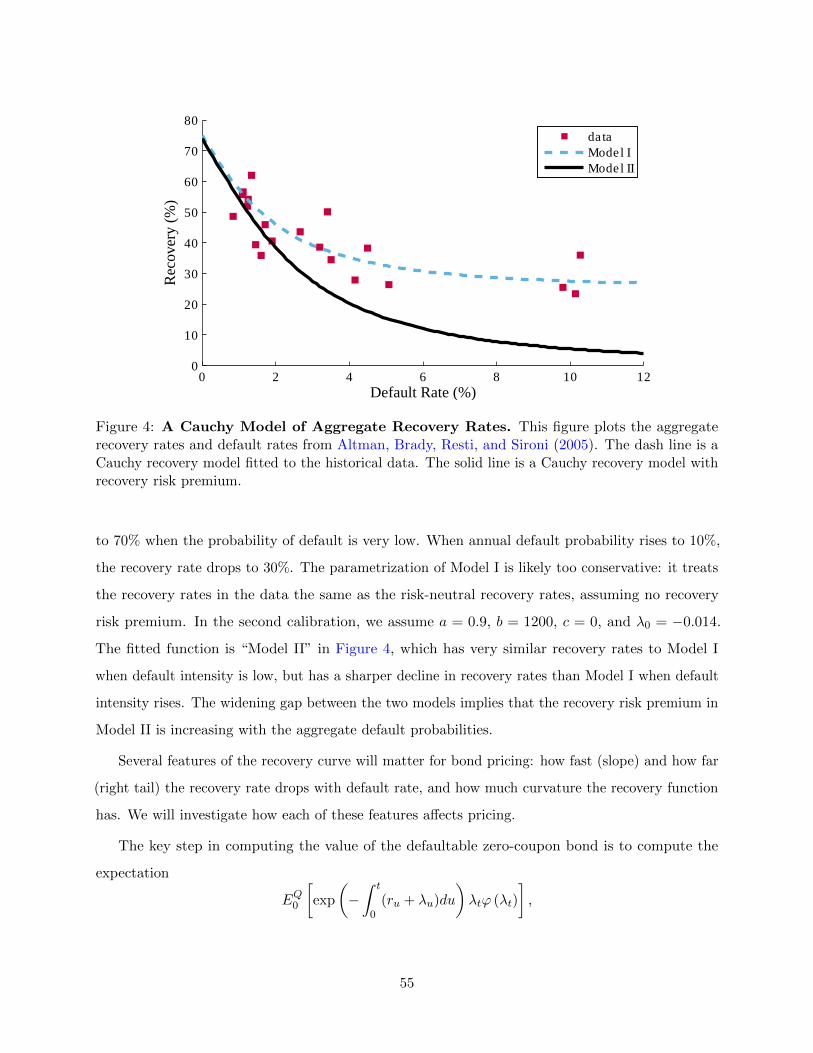
0 2 4 6 8 10 120
10
20
30
40
50
60
70
80
Default Rate (%)
Rec
ov
ery
(%
)
data
Model I
Model II
Figure 4: A Cauchy Model of Aggregate Recovery Rates. This figure plots the aggregaterecovery rates and default rates from Altman, Brady, Resti, and Sironi (2005). The dash line is aCauchy recovery model fitted to the historical data. The solid line is a Cauchy recovery model withrecovery risk premium.
to 70% when the probability of default is very low. When annual default probability rises to 10%,
the recovery rate drops to 30%. The parametrization of Model I is likely too conservative: it treats
the recovery rates in the data the same as the risk-neutral recovery rates, assuming no recovery
risk premium. In the second calibration, we assume a = 0.9, b = 1200, c = 0, and λ0 = −0.014.
The fitted function is “Model II” in Figure 4, which has very similar recovery rates to Model I
when default intensity is low, but has a sharper decline in recovery rates than Model I when default
intensity rises. The widening gap between the two models implies that the recovery risk premium in
Model II is increasing with the aggregate default probabilities.
Several features of the recovery curve will matter for bond pricing: how fast (slope) and how far
(right tail) the recovery rate drops with default rate, and how much curvature the recovery function
has. We will investigate how each of these features affects pricing.
The key step in computing the value of the defaultable zero-coupon bond is to compute the
expectation
EQ0
[exp
(−∫ t
0(ru + λu)du
)λtϕ (λt)
],
55

Table 1: Calibration of the Risk-Neutral dynamics of λ and Y
κλ θλ σλ κY θY σY δ
-0.035 -0.08 0.07 0.02 0.10 0.06 0.1
which is mapped into the generalized transform of Theorem 1 by choosing
f (α ·X) = ι1 ·X,
g (β ·X) =a
1 + b(ι1 ·X − λ0)2,
where ι1 = [1 0]′.
It is straightforward to use the recovery model ϕ(X) to price other credit products, such as credit
default swaps or recovery locks. In addition, our model can be generalized to allow for violations of
the no-jump conditions.33 Thus, it can be used in models with flight-to-quality, default contagion,
systematic jump risk, or other features that violate the no-jump condition.
We now use the processes of default intensity λt and riskfree rate rt (105–107) and the recovery
model (108) to price a 5-year defaultable zero-coupon bond of a representative firm, which has the
same default intensity as the aggregate intensity λt. We calibrate the process of λt and Yt under
the risk-neutral measure following Duffee (1999). The parameter values are reported in Table 1.
Notice that κλ < 0, which is consistent with Duffee’s finding that the default intensity of a typical
firm is nonstationary under the risk-neutral measure.
The results are reported in Figure 5. The top panels investigate Stochastic Recovery Model I,
where the recovery function is fitted to the historical recovery rates (no recovery risk premium);
the bottom panels investigate Stochastic Recovery Model II, which assumes that the recovery risk
premium increases with aggregate default intensity (see Figure 4). A popular assumption for default
recovery in both academic analysis and industry practice is to assume 75% constant loss rate (see
e.g., Pan and Singleton (2008)). This value is higher than the historical mean loss rate, which is a
parsimonious way to capture the recovery risk premium. Thus, for comparison, we also report the
results for two alternative models: (1) recovery of market value (RMV), with constant loss rate
33We can either explicitly make the correction for jumps as in Duffie, Schroder, and Skiadas (1996), or use thechange-of-measure method in Collin-Dufresne, Goldstein, and Hugonnier (2004).
56

0 2 4 6 8 100
200
400
600
800
1000S
pre
ad (
bps)
Default Intensity (%)
A. Model I: Credit Spreads
RMV (L = 75%)RFV (L = 75%)Stochastic Recovery
0 2 4 6 8 10−80
−60
−40
−20
0
Perc
enta
ge
Default Intensity (%)
B. Model I: Pricing Error
RMV (L = 75%)RFV (L = 75%)
0 2 4 6 8 100
200
400
600
800
1000
1200
Spre
ad (
bps)
Default Intensity (%)
C. Model II: Credit Spreads
RMV (L = 75%)RFV (L = 75%)Stochastic Recovery
0 2 4 6 8 10−60
−40
−20
0
20
40
Perc
enta
ge
Default Intensity (%)
D. Model II: Pricing Error
RMV (L = 75%)RFV (L = 75%)
Figure 5: Credit spreads for 5-year bonds with constant recovery and Cauchy recovery.For different values of conditional default intensity, this figure plots the credit spreads of a 5-year zero-coupon
defaultable bond, and the pricing errors of the RMV and RFV model with constant recovery rates relative to
two versions of the stochastic recovery model. “RMV” stands for “recovery of market value”; “RFV” stands
for “recovery of face value”.
L = 0.75; (2) recovery of face value (RFV), with constant loss rate L = 0.75.
Panel A shows that, without the recovery risk premium, the credit spreads generated by the
stochastic recovery model are lower than the RMV and RFV model with constant recovery rate.
Panel B reports the pricing errors of the RMV and RFV model relative to the stochastic recovery
model (assuming the latter is the true model), computed as
stochastic recovery yield− constant recovery yield
stochastic recovery yield− default-free yield.
As expected, if there is no recovery risk premium (as in Model I), the main concern of the constant
recovery assumption is underpricing, i.e. they generate credit spreads that are too high. The pricing
57

errors are large. For example, the pricing errors of the RMV model are at least 20%, and can be
over 40% when default intensity is low (< 2%).
The results are quite different for Stochastic Recovery Model II. As shown in Panel C, the credit
spreads generated by Model II are visibly more convex than the spreads from the RMV or RFV
model with constant recovery rate. When default intensity is low, credit spreads are lower for the
stochastic recovery model, because the conditional recovery rates are higher than under the constant
recovery assumption. As aggregate default intensity rises, the size of the recovery risk premium
increases, which lowers the risk-neutral recovery rates and explains the rapid rise in the spreads of
Model II.
Panel D gives us a better sense of the size of pricing errors. When the aggregate default intensity
is low, the recovery risk premium is small. Thus, the assumption of a 25% constant recovery rate
during these times would be too “conservative”, which makes the RMV model generate spreads
that are too high. The pricing errors can be well over 20% for low values of λ. On the contrary,
at times when the aggregate default rates are high, the assumption of 25% constant recovery rate
becomes too optimistic. In fact, for λ > 2.5%, the spreads in Model II exceed those in the RMV
model. The pricing errors are over 10% for λ > 4.5%, and can be as high as 20% when the default
intensity reaches 10%.
There is another important message in Figure 5. The curvature in the graphs of the spreads
and pricing errors suggests that simply adjusting the constant recovery rate in the RMV model
does not solve the mispricing problem. Changing the recovery rate amounts to (approximately)
parallel-shifting the spreads or pricing errors, and will either exacerbate the underpricing for low
λ or overpricing for high λ. These results suggest that it is important to dynamically account for
the negative correlation between default intensity and recovery rate when pricing credit-sensitive
securities.
F Labor income risk
This section provides more details on the calibration and analysis of the model with time-varying
labor income risk.
The parameters are summarized in Table 2 and are calibrated as follows. We set the long-run
mean growth rate of labor income and dividends to 1.5%. We specify the long run labor income
58

γ 6 ρ`,d -30.3%ρ 1% σ` 5.4%g 1.5% σd 11.1%
S 80% σ∞(ρ`,d) 9.8%a 1
3 σ∞(σ`) 0.0018%κs 0.0231 σ∞(σd) 0.017%κV 0.0693 σSS(V ) 1.07
Table 2: Parameters. This table gives the parameters and moments used to calibrate the model. The left
column gives the preference parameters and conditional mean parameters for the process. The right column
gives the conditional moments used to calibrate the parameters (Σ0,Σ1). The first three calibration moments
refer to the steady state values. The next three refer to the conditional volatility of the conditional moments
evaluated at the long run mean of V . σ(σd) is the steady state volatility of σd. V is normalized to be one.
share, S, to be 75%. As the covariance parameters (Σ0 and Σ1) are difficult to directly interpret, we
calibrate them by considering their effect on the volatility of labor income, the volatility of dividends,
and their correlation. We set the parameters so that when Vt is at its long run mean V (which
is normalized to be one), (σ`,t, σd,t, ρ`,d,t) are given by σ` = 5.4%, σd = 11.1%, and ρ`,d = −30.3%
respectively. Note that due to CRRA utility, our model presents the equity premium-risk free rate
puzzle (Mehra and Prescott (1983)), and we choose our parameterization to generate higher premium
with reasonable risk aversion by slightly overstating the volatility of labor income relative to the
data, with the ratio of dividend to labor income volatility qualitatively similar to Lettau, Ludvigson,
and Wachter (2008). We also calibrate the volatility of (σd, σ`, ρ`,d) when Vt is at its long run mean,
which we denote with by σ∞(σd) = 1.7bp, σ∞(σ`) = 0.18bp, and σ∞(ρ`,d) = 9.8%. Finally, we
calibrate the volatility of V in the steady state distribution, which we denote by σSS(V ), to be 1.07.
Taken together, these 7 moments (along with the simplifying assumption that innovations to V are
uncorrelated with innovations to either ` or d) fix the free parameters in Σ0 (3 parameters) and Σ1
(4 parameters). Under this calibration, when V is at the highest (lowest) decile, the volatility of
labor income is 6% (5%), the volatility of dividends is 16%(6%) and their correlation is -10% (-80%).
The volatility parameters where chosen to qualitatively match the variation found in Figure 2.
Next, we investigate the price of risk for shocks to dividends and labor income, which are
transparent and helpful for our understanding of the risk premiums on financial wealth and human
capital. From the stochastic discount factor, we can compute the price of dividend risk, which is
59

0 1 2 3 40
200
400
600
800
1000
1200
1400
A. Distribution of volatility factor
√Vt
0 0.2 0.4 0.6 0.8 10
200
400
600
800
1000
1200
1400
1600
1800B. Distribution of labor share
Lt/Ct
Figure 6: Simulated distributions. Panels A and B plot the simulated distributions of the volatility
factor√Vt and labor share Lt/Ct.
defined as the risk premium for one unit exposure to dividend shocks:
PRdt =γcovt(ct, dt)
σd,t= γ
(LtCtρtσ`,t +
(1− Lt
Ct
)σd,t
), (110)
where ct is log consumption; σ`,t and σd,t are the conditional volatilities of labor income and
dividends, with their dependence on the volatility factor Vt captured by the time subscripts. On the
one hand, holding Vt constant (so that σ`,t, σd,t, and ρt are all constant), the price of dividend risk
will rise as labor share falls as long as σd,t > ρtσ`,t (for example, when dividends are more volatile
than labor income or when their correlation is negative), which is the composition effect highlighted
in SV. On the other hand, holding labor share fixed, as Vt increases, the volatility of labor income,
dividends, and the correlation between the two will increase. All three factors contribute to raise
the price of dividend risk. Intuitively, investors become more reluctant to hold financial assets either
when there is less labor income to buffer the financial shocks (lower labor share), or when labor
income becomes a worse hedge against the financial shocks (higher correlation or higher volatility of
labor income).
Finally, if the correlation between labor income and dividends is sufficiently negative and the
labor share is sufficiently high, the price of dividend risk can become negative. This is because when
the investor is heavily exposed to labor income risk and ρt is close to −1, bad news for dividends will
60

tend to be accompanied by good news to labor income, which causes consumption to rise (opposite
to dividends).
Similarly, the price of labor income risk measures the risk premium for one unit exposure to
labor income shocks:
PR`t =γcovt(ct, `t)
σ`,t= γ
(LtCtσ`,t +
(1− Lt
Ct
)ρtσd,t
). (111)
Provided that σ`,t > ρtσd,t (for example, when the correlation is very small or negative), the price
of labor income risk will rise with labor share. Also, holding the labor share constant, the price of
labor income risk unambiguously falls as the correlation and volatilities fall.
Figure 7 shows the quantitative effects of the labor share and correlation (volatility) on the price
of dividend risk and labor income risk. First, we show how the volatilities of labor income, dividends,
and the correlation between the two are tied to the volatility factor Vt. As Panel A shows, both
the volatility of labor income and dividends are monotonically increasing in the volatility factor,
although dividend volatility varies significantly more than does labor income. This property is an
important feature of our model, which is also consistent with the data. In Panel B, the conditional
correlation between labor income and dividends is also monotonically increasing in the volatility
factor. Since the volatilities and correlation are all monotonic functions of the volatility factor Vt,
without loss of generality we use the correlation ρt in place of Vt in the plots for the remainder of
the paper.
As Panels C and D show, holding the correlation constant, the price of dividend risk is decreasing
in labor share, while the price of labor income risk is increasing in the labor share. When holding
the labor share constant, both prices of risk increase with the correlation between labor income and
dividends (the volatility factor). These features are consistent with our analysis above.
Notice also that while the price of dividend risk is always falling as the labor share rises,
the decline is less pronounced when the correlation (volatility) is small. For example, when the
correlation is -0.1, the price of dividend risk falls from 0.36 to 0.06 as labor share rises from 0.6 to
0.9; when the correlation is -0.8, price of dividend risk falls from 0.01 to -0.17 for the same increase
in labor share. The opposite is true for the price of labor income risk. From (110) and (111) we see
that the sensitivity of PRdt to Lt/Ct is σd,t − ρtσ`,t, which is increasing in Vt under our calibration,
whereas the sensitivity PR`t to Lt/Ct is σ`,t − ρtσd,t, which is decreasing in Vt under our calibration.
61
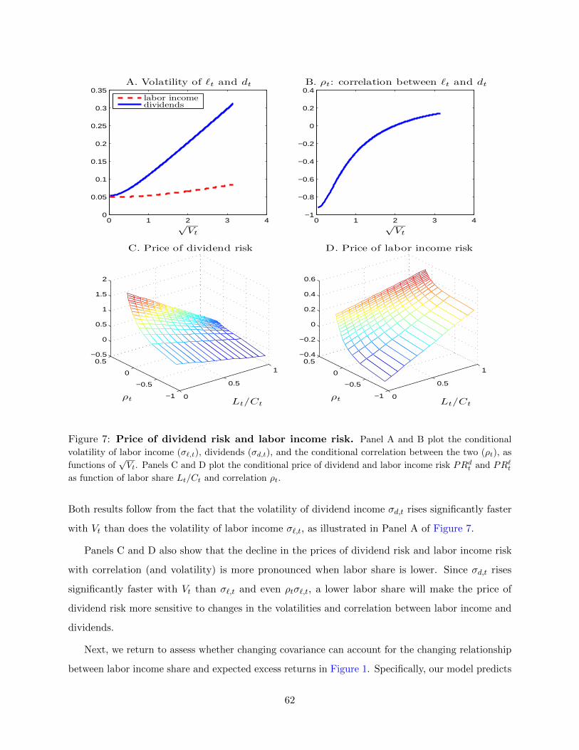
0 1 2 3 40
0.05
0.1
0.15
0.2
0.25
0.3
0.35
√Vt
A. Volatility of ℓt and dt
labor incomedividends
0 1 2 3 4−1
−0.8
−0.6
−0.4
−0.2
0
0.2
0.4
√Vt
B. ρt: correlation between ℓt and dt
0
0.5
1
−1
−0.5
0
0.5
−0.5
0
0.5
1
1.5
2
Lt/Ct
C. Price of dividend risk
ρt 0
0.5
1
−1
−0.5
0
0.5
−0.4
−0.2
0
0.2
0.4
0.6
Lt/Ct
D. Price of labor income risk
ρt
Figure 7: Price of dividend risk and labor income risk. Panel A and B plot the conditional
volatility of labor income (σ`,t), dividends (σd,t), and the conditional correlation between the two (ρt), as
functions of√Vt. Panels C and D plot the conditional price of dividend and labor income risk PRd
t and PR`t
as function of labor share Lt/Ct and correlation ρt.
Both results follow from the fact that the volatility of dividend income σd,t rises significantly faster
with Vt than does the volatility of labor income σ`,t, as illustrated in Panel A of Figure 7.
Panels C and D also show that the decline in the prices of dividend risk and labor income risk
with correlation (and volatility) is more pronounced when labor share is lower. Since σd,t rises
significantly faster with Vt than σ`,t and even ρtσ`,t, a lower labor share will make the price of
dividend risk more sensitive to changes in the volatilities and correlation between labor income and
dividends.
Next, we return to assess whether changing covariance can account for the changing relationship
between labor income share and expected excess returns in Figure 1. Specifically, our model predicts
62

Table 3: Return Forecasting Regressions. Dependent variable: cumulative excess return on the
market over various horizons (quarters). Predictive variable Lt/Ct: share of labor income to consumption.
The first set of t-stats is the Newey-West adjusted t-statistics, with the number of lags double the forecasting
horizon. The second set of t-stats is the Hansen-Hodrick adjusted t-statistics using the same number of lags
as the Newey-West t-stats.
Panel A: 1947-1990 Panel B: 1991-2010
4 8 12 16 4 8 12 16
Lt/Ct -1.042 -2.440 -4.257 -6.263 3.621 7.233 11.342 15.791t-stat (NW) -1.890 -3.664 -4.367 -4.396 1.948 2.185 2.569 3.637t-stat (HH) -1.086 -1.401 -1.900 -2.330 1.295 1.406 1.531 1.724Adj. R2 0.041 0.125 0.270 0.406 0.101 0.214 0.286 0.363
that the labor income share has little effect on the equity premium when consumption volatility
and the correlation between labor income and dividends are low.
In Table 3, we formally examine the difference of return predictability with labor share in the
two samples using regressions of long-horizon excess returns on lagged labor shares. The specific
form of the regression is
rxt,t+K = β0(K) + β1(K)LtCt
+ εt+K , (112)
where rxt,t+K is the cumulative excess return on the market over K quarters, and we consider
K = 4, 8, 12, 16. For each regression, we report the point estimates of β1(K), the NeweyWest
corrected t-statistics (with the number of lags equal to 2K, as in SV), the Hansen-Hodrick corrected
t-statistics and the adjusted R2.
The regression results are consistent with what we have inferred from Figure 1. Labor share
significantly predicts long-horizon returns with a negative sign in the period 1947-1990, which
confirms the findings of SV. In the post-1990 period, the regression coefficients on labor share
become positive, although they are statistically non-significant at all horizons when using the
Hansen-Hodrick standard errors. Based on the moving-window estimates of consumption volatility
and correlation between labor income and dividends in Figure 2, volatilities and correlation are both
higher pre-1990, which according to our model implies a stronger composition effect (risk premium
falls as labor share rises) during this period. As both the volatilities and correlation become smaller
in the second sample, the composition effect should indeed become weaker.
On the other hand, in Table 3 the point estimate of the regression coefficients are economically
63

large and significantly positive at longer horizons with respect to the Newey-West standard errors.
What could explain such a possible change in the predictive power of labor share? It is possible
that some variable that is driving the risk premium on stocks has become correlated with labor
share (or happens to be correlated in the relatively short sample). For example, observe that over
this period, labor share and covariance are generally positively correlated in Figure 2. In this case,
according to Figure 3, decreasing share may be associated with decreasing risk premium due to
declining correlation, despite the reverse univariate relationship where covariance is held fixed. Put
differently, our covariance variable, Vt, may represent a variable which is correlated with both the
regressor and the residual in (112), resulting in biased estimates. Other risks factors may also be at
play as well. For example, the correlation between labor share and the consumption-wealth measure
CAY (see Lettau and Ludvigson (2001b)) is −0.15 over the period 1952-2010, but jumps to 0.6 in
the period 1990-2010. Thus, the fact that CAY predicts the equity risk premium with a positive
sign can help explain the regression results in the post-1990 period as well. These possibilities could
be explored further by expanding our framework to include the additional covariates.
64