Generalized Krasnoselskii-Mann-type Iterations forNonexpansive Mappings in Hilbert Spaces

Christian Kanzow∗ and Yekini Shehu†

August 1, 2016

Abstract

The Krasnoselskii-Mann iteration plays an important role in the approxima-tion of fixed points of nonexpansive operators; it is is known to be weaklyconvergent in the infinite dimensional setting. In this present paper, we pro-vide a new inexact Krasnoselskii-Mann iteration and prove weak convergenceunder certain accuracy criteria on the error resulting from the inexactness. Wealso show strong convergence for a modified inexact Krasnoselskii-Mann iter-ation under suitable assumptions. The convergence results generalize existingones from the literature. Applications are given to the Douglas-Rachford split-ting method, the Fermat-Weber location problem as well as the alternatingprojection method by John von Neumann.

1 Introduction

Let X be a normed space and T : X → X be a nonexpansive mapping, i.e., Tsatisfies

‖Tx− Ty‖ ≤ ‖x− y‖ ∀x, y ∈ X.

We further denote the set of fixed points of T by

F (T ) := {x ∈ X | Tx = x}.

Note that, if T is actually a mapping from X to a subset K ⊆ X, then F (T )automatically belongs to K. Prominent examples for nonexpansive mappings froma Hilbert space X to a nonempty, closed, and convex set K ⊆ X are, for example,the projection map, the proximal point map, and several composite maps whichinvolve at least one of these two mappings, see, e.g., [2] for more details.

Throughout this paper, we consider the real Hilbert space setting: H denotes areal Hilbert space with scalar product 〈., .〉 and induced norm ‖·‖. Our aim is to find

∗University of Wurzburg, Institute of Mathematics, Campus Hubland Nord, Emil-Fischer-Str.30, 97074 Wurzburg, Germany; e-mail: kanzow@mathematik.uni-wuerzburg.de†University of Nigeria, Department of Mathematics, Nsukka, Nigeria; e-mail:

yekini.shehu@unn.edu.ng. Current address (May 2016 – April 2018): University of Wurzburg, In-stitute of Mathematics, Campus Hubland Nord, Emil-Fischer-Str. 30, 97074 Wurzburg, Germany.The research of this author is supported by the Alexander von Humboldt-Foundation.

1

a fixed point of a nonexpansive mapping T defined on H. Existence and uniquenessresults as well as many iterative schemes are well-known from the literature, cf.[3, 5, 6, 7] and references therein for some relevant results in this direction. Inparticular, one of the most famous fixed point methods is the Krasnoselskii-Manniteration from [19, 24] that starts at some given point x1 ∈ H and uses the recursion

xn+1 = (1− λn)xn + λnTxn ∀n = 1, 2, . . . (1)

for some suitably chosen scalars λn ∈ [0, 1]. The most general convergence resultfor this procedure is due to Reich [26] and assumes that F (T ) is nonempty and thescalars λn satisfy the condition

∞∑n=1

λn(1− λn) =∞, (2)

then the iterates {xn} converge weakly to a fixed point of T . This statement remainstrue if T : K → K with a nonempty, closed, and convex set K ⊆ H, in which case itfollows immediately from (1) that the whole sequence {xn} remains in K providedthat the starting point x1 is chosen from K.

Strong convergence of the Krasnoselskii-Mann iteration cannot be expected ingeneral, as noted by a counterexample in [15]. On the other hand, there exist acouple of modified schemes which guarantee strong convergence results, see [5, 8] fordifferent examples. One of these schemes uses the recursion

xn+1 := αnxn + βnTxn + δnu, (3)

where T : H → K is nonexpansive, K ⊆ H is nonempty, closed, and convex,αn, βn, δn ∈ [0, 1] are suitably chosen scalars satisfying αn + βn + δn = 1, and udenotes a fixed element from K; for more details and conditions on the choice ofαn, βn, δn, we refer to [9, 10, 18, 28] and the discussion in Section 4.

The overall convergence behaviour of the Krasnoselskii-Mann iteration from (1)is therefore well-investigated and yields very satisfactory global convergence results.On the other hand, this theory requires that T can be evaluated exactly. In general,this is an unrealistic assumption because the evaluation of T might involve the com-putation of a projection or the solution of a nonlinear (convex) program. Combettes[11] therefore considers the convergence of the inexact Krasnoselskii-Mann iteration

xn+1 := (1− λn)xn + λn(Txn + en) (4)

with a given starting point x1 ∈ H, where en represents an error in the evaluationof Txn. He proves weak convergence of the sequence {xn} under the assumptionsthat F (T ) is nonempty, λn ∈ (0, 1) satisfies (2), and the additional error condition

∞∑n=1

λn‖en‖ <∞.

The same inexact Krasnoselskii-Mann scheme has been investigated recently byLiang et al. [20] where additional results are presented, in particular, suitable rateof convergence results are provided.

2

Apart from the error due to the inexact evaluation of T , implementations of theKrasnoselskii-Mann iteration produce an additional error due to the finite precisionarithmetic of the computer. To get a complete picture of the practical numericalbehaviour of the Krasnoselskii-Mann iteration, we are therefore forced to analysethe convergence properties of a scheme like

xn+1 := (1− λn)xn + λn(Txn + en) + en,

where, again, en represents the error in the evaluation of Txn, whereas en denotesthe error resulting from the finite precision arithmetic. To keep the notation simple,we can write this as

xn+1 := (1− λn)xn + λnTxn + rn

for some vector rn that we call the residual since it represents the difference betweenthe exact Krasnoselskii-Mann iteration and its inexact counterpart.

Here we consider the more general inexact scheme

xn+1 := αnxn + βnTxn + rn, (5)

where αn, βn ∈ [0, 1] are suitable numbers satisfying αn + βn ≤ 1, hence these twonumbers do not necessarily sum up to one, and rn is again called the residual vector.Despite the fact that this generalizes existing choices, it turns out in our subsequentanalysis that, to some extent, the particular choice αn +βn < 1 also bridges the gapbetween weak and strong convergence results.

Sometimes it is more convenient to consider the recursion

xn+1 := αnxn + βnTxn + γnen, (6)

whereαn, βn, γn ∈ [0, 1] satisfy αn + βn + γn = 1 (7)

and the vector en is called the error. Note that this iterative scheme is a special caseof (5) simply by setting rn = γnen. Our aim is to prove weak and strong convergenceresults for these modified inexact Krasnoselskii-Mann iterations under suitable as-sumptions which generalize the conditions known for the previously mentioned exactand inexact versions of this fixed-point method.

The paper is therefore organized as follows: We first recall some basic definitionsand results in Section 2. The weak convergence of the iterative scheme from (5)(and its special instance from (6), (7)) is then investigated in Section 3. Strongconvergence of a modified version is shown in Section 4. An application to theDouglas-Rachford splitting method, the Fermat-Weber location problem, and thealternating projection method by John von Neumann can be found in Section 5.We conclude with some final remarks in Section 6.

Notation: Given a Hilbert space H, we denote by 2H the power set of H. Anoperator A : H → 2H is sometimes called a multi-function. Given such a multi-function, we write zer(A) for the set {x ∈ H | 0 ∈ Ax}. The projection of anelement x ∈ H onto a nonempty, closed, and convex set C ⊆ H is denoted by PCx.

3

2 Preliminaries

Here we state some basic properties that will be used in our convergence theorems.We begin with the following lemma whose proof is elementary and therefore omitted.

Lemma 2.1. Let X be a real inner product space. Then the following statementshold:

(a) ‖x+ y‖2 ≤ ‖x‖2 + 2〈y, x+ y〉, ∀x, y ∈ X.

(b) ‖tx+ sy‖2 = t(t+ s)‖x‖2 + s(t+ s)‖y‖2 − st‖x− y‖2, ∀x, y ∈ X, ∀s, t ∈ R.

The following result is also well-known, see, e.g., [1]. It plays a central role in ourweak convergence result.

Lemma 2.2. Let {σn} and {γn} be nonnegative sequences satisfying∞∑n=1

σn < ∞

and γn+1 ≤ γn + σn, n = 1, 2, . . .. Then, {γn} is a convergent sequence.

The next result comes from [30] and will be exploited in our strong convergenceresult.

Lemma 2.3. Let {an} be a sequence of nonnegative real numbers satisfying thefollowing relation:

an+1 ≤ (1− αn)an + αnσn + γn, n ≥ 1,

where

(a) {αn} ⊂ [0, 1],∑∞

n=1 αn =∞;

(b) lim supσn ≤ 0;

(c) γn ≥ 0 (n ≥ 1),∑∞

n=1 γn <∞.

Then, an → 0 as n→∞.

Let H be a real Hilbert space with inner product 〈., .〉 and norm ‖.‖, and let K bea nonempty, closed, and convex subset of H.

For any point u ∈ H, there exists a unique point PKu ∈ K such that

‖u− PKu‖ ≤ ‖u− y‖, ∀y ∈ K.

PK is called the metric projection of H onto K. We know that PK is a nonexpansivemapping of H onto K. More precisely, PK is known to be firmly nonexpansive inthe sense that

〈x− y, PKx− PKy〉 ≥ ‖PKx− PKy‖2 (8)

for all x, y ∈ H. Furthermore, PKx is characterized by the properties PKx ∈ K and

〈x− PKx, PKx− y〉 ≥ 0, ∀y ∈ K. (9)

We finally restate an important result which is due to Opial [25] and characterizesthe weak limit of a weakly convergent sequence in a Hilbert space.

4

Theorem 2.4. (Opial)Let H be a Hilbert space and {xn} be any sequence in H converging weakly to x.Then the strict inequality

lim infn→∞

‖xn − x‖ < lim infn→∞

‖xn − y‖

holds for all y 6= x.

An operator A : H → 2H with domain D(A) is said to be monotone if

〈u− v, x− y〉 ≥ 0 ∀x, y ∈ D(A), u ∈ Ax, v ∈ Ay.

We say that the monotone operator A is maximal monotone if its graph

G(A) := {(x, y) : x ∈ D(A), y ∈ Ax}

is not properly contained in the graph of any other monotone operator.

3 Weak Convergence

This section investigates the weak convergence properties of the generalized inex-act Krasnoselskii-Mann iteration from (5). The following is the main convergenceresult and shows that we re-obtain the classical weak convergence of the exactKrasnoselskii-Mann iteration under suitable conditions on the choice of αn, βn andthe behaviour of rn. These conditions will be discussed in some more detail afterthe proof of this result.

Theorem 3.1. Let K be a nonempty, closed, and convex subset of a real Hilbertspace H. Suppose that T : H → K is a nonexpansive mapping such that its set offixed points F (T ) is nonempty. Let the sequence {xn} in H be generated by choosingx1 ∈ H and using the recursion

xn+1 := αnxn + βnTxn + rn, ∀n ≥ 1, (10)

where rn denotes the residual vector. Here we assume that {αn} and {βn} are realsequences in [0, 1] such that αn + βn ≤ 1 for all n ≥ 1 and the following conditionshold:

(a)∞∑n=1

αnβn =∞;

(b)∞∑n=1

‖rn‖ <∞;

(c)∞∑n=1

(1− αn − βn) <∞.

Then the sequence {xn} generated by (10) converges weakly to a fixed point of T .

5

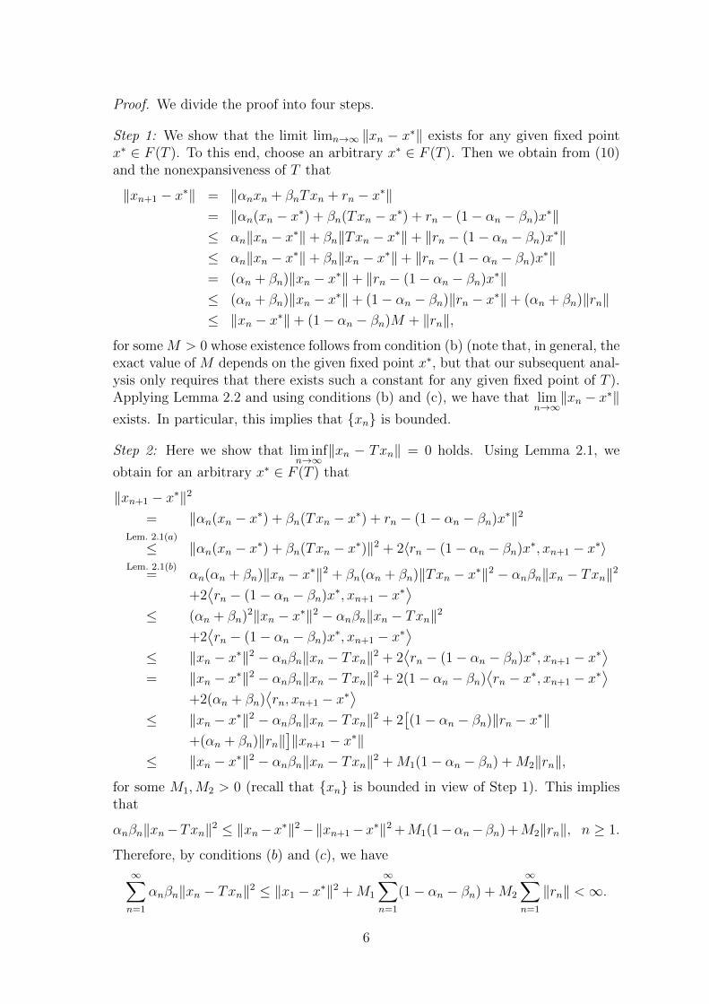
Proof. We divide the proof into four steps.

Step 1: We show that the limit limn→∞ ‖xn − x∗‖ exists for any given fixed pointx∗ ∈ F (T ). To this end, choose an arbitrary x∗ ∈ F (T ). Then we obtain from (10)and the nonexpansiveness of T that

‖xn+1 − x∗‖ = ‖αnxn + βnTxn + rn − x∗‖= ‖αn(xn − x∗) + βn(Txn − x∗) + rn − (1− αn − βn)x∗‖≤ αn‖xn − x∗‖+ βn‖Txn − x∗‖+ ‖rn − (1− αn − βn)x∗‖≤ αn‖xn − x∗‖+ βn‖xn − x∗‖+ ‖rn − (1− αn − βn)x∗‖= (αn + βn)‖xn − x∗‖+ ‖rn − (1− αn − βn)x∗‖≤ (αn + βn)‖xn − x∗‖+ (1− αn − βn)‖rn − x∗‖+ (αn + βn)‖rn‖≤ ‖xn − x∗‖+ (1− αn − βn)M + ‖rn‖,

for some M > 0 whose existence follows from condition (b) (note that, in general, theexact value of M depends on the given fixed point x∗, but that our subsequent anal-ysis only requires that there exists such a constant for any given fixed point of T ).Applying Lemma 2.2 and using conditions (b) and (c), we have that lim

n→∞‖xn − x∗‖

exists. In particular, this implies that {xn} is bounded.

Step 2: Here we show that lim infn→∞

‖xn − Txn‖ = 0 holds. Using Lemma 2.1, we

obtain for an arbitrary x∗ ∈ F (T ) that

‖xn+1 − x∗‖2

= ‖αn(xn − x∗) + βn(Txn − x∗) + rn − (1− αn − βn)x∗‖2Lem. 2.1(a)

≤ ‖αn(xn − x∗) + βn(Txn − x∗)‖2 + 2〈rn − (1− αn − βn)x∗, xn+1 − x∗〉Lem. 2.1(b)

= αn(αn + βn)‖xn − x∗‖2 + βn(αn + βn)‖Txn − x∗‖2 − αnβn‖xn − Txn‖2

+2⟨rn − (1− αn − βn)x∗, xn+1 − x∗

⟩≤ (αn + βn)2‖xn − x∗‖2 − αnβn‖xn − Txn‖2

+2⟨rn − (1− αn − βn)x∗, xn+1 − x∗

⟩≤ ‖xn − x∗‖2 − αnβn‖xn − Txn‖2 + 2

⟨rn − (1− αn − βn)x∗, xn+1 − x∗

⟩= ‖xn − x∗‖2 − αnβn‖xn − Txn‖2 + 2(1− αn − βn)

⟨rn − x∗, xn+1 − x∗

⟩+2(αn + βn)

⟨rn, xn+1 − x∗

⟩≤ ‖xn − x∗‖2 − αnβn‖xn − Txn‖2 + 2

[(1− αn − βn)‖rn − x∗‖

+(αn + βn)‖rn‖]‖xn+1 − x∗‖

≤ ‖xn − x∗‖2 − αnβn‖xn − Txn‖2 +M1(1− αn − βn) +M2‖rn‖,

for some M1,M2 > 0 (recall that {xn} is bounded in view of Step 1). This impliesthat

αnβn‖xn−Txn‖2 ≤ ‖xn−x∗‖2−‖xn+1−x∗‖2 +M1(1−αn−βn) +M2‖rn‖, n ≥ 1.

Therefore, by conditions (b) and (c), we have

∞∑n=1

αnβn‖xn − Txn‖2 ≤ ‖x1 − x∗‖2 +M1

∞∑n=1

(1− αn − βn) +M2

∞∑n=1

‖rn‖ <∞.

6

Using assumption (a), we obtain lim infn→∞

‖xn − Txn‖ = 0.

Step 3: We now show that we actually have limn→∞‖xn − Txn‖ = 0. To this end, first

observe that

xn+1 − xn = βn(Txn − xn) + rn − (1− αn − βn)xn. (11)

This implies

‖Txn+1 − xn+1‖= ‖Txn+1 − Txn + Txn − (αnxn + βnTxn + rn)‖= ‖Txn+1 − Txn + (1− βn)(Txn − xn)− rn + (1− αn − βn)xn‖≤ ‖Txn+1 − Txn‖+ (1− βn)‖Txn − xn‖+ ‖(1− αn − βn)xn − rn‖≤ ‖xn+1 − xn‖+ (1− βn)‖Txn − xn‖+ ‖(1− αn − βn)xn − rn‖(11)= ‖Txn − xn‖+ 2‖(1− αn − βn)xn − rn‖≤ ‖Txn − xn‖+ 2(1− αn − βn)‖xn‖+ 2‖rn‖≤ ‖Txn − xn‖+ 2‖rn‖+ 2M3(1− αn − βn),

for some M3 > 0. Observe from conditions (b) and (c) that 2∞∑n=1

(‖rn‖ + M3(1 −

αn − βn))<∞. Applying Lemma 2.2 to the last chain of inequalities, we have that

limn→∞‖xn − Txn‖ exists. In view of Step 2, this yields lim

n→∞‖xn − Txn‖ = 0.

Step 4: In this final step, we prove the weak convergence of the sequence {xn} to afixed point of T . Since {xn} is bounded by Step 1, there exists a subsequence {xnk

}of {xn} that converges weakly to some element p. We first show that p ∈ F (T ).Assume the contrary that p 6= Tp. Using Opial’s Theorem 2.4 and the fact thatlimn→∞‖xn − Txn‖ = 0 by Step 3, we get

lim infn→∞

‖xnk− p‖ < lim inf

n→∞‖xnk

− Tp‖

≤ lim infn→∞

(‖xnk

− Txnk‖+ ‖Txnk

− Tp‖)

= lim infn→∞

‖Txnk− Tp‖

≤ lim infn→∞

‖xnk− p‖.

This contradiction shows that p ∈ F (T ). Suppose that the whole sequence {xn}does not converge weakly to p. Then there exists another subsequence {xmj

} of{xn} which converges weakly to some q 6= p. As in in the case of p we must haveq ∈ F (T ). It therefore follows from Step 1 that lim

n→∞‖xn − p‖ and lim

n→∞‖xn − q‖

exist. Let us denote these limits by d1 := limn→∞‖xn − p‖ and d2 := lim

n→∞‖xn − q‖,

respectively. Exploiting Opial’s Theorem 2.4 once again, we obtain

d1 = lim infk→∞

‖xnk− p‖ < lim inf

k→∞‖xnk

− q‖ = d2

= lim infj→∞

‖xmj− q‖ < lim inf

j→∞‖xmj

− p‖ = d1,

which is a contradiction. Therefore, p = q and the entire sequence {xn} convergesweakly to p. This completes the proof.

7

Let us discuss Theorem 3.1 to some extent in the following remark.

Remark 3.2. (a) Consider the exact Krasnoselskii-Mann iteration from (1) whichcorresponds to the case rn = 0 as well as αn = 1− λn, βn = λn for suitable numbersλn ∈ [0, 1]. It then follows that conditions (b) and (c) in Theorem 3.1 are automati-cally satisfied. Furthermore, condition (a) reduces to (2), i.e. we re-obtain the usualassumption for the convergence of the Krasnoselskii-Mann iteration as a special caseof our Theorem 3.1.

(b) Next consider the inexact Krasnoselskii-Mann iteration from (4) proposed byCombettes [11]. This is also a special case of our recursion (10) by setting αn :=1− λn, βn := λn, and rn := λnen. It follows that condition (c) in Theorem 3.1 holdsautomatically, whereas conditions (a) and (b) become

∞∑n=1

λn(1− λn) =∞ and∞∑n=1

λn‖en‖ <∞,

which are precisely the convergence assumptions used by Combettes [11] (formally,Combettes assumes that λn ∈ (0, 1), whereas here λn can be taken from the closedinterval [0, 1]).

(c) Recall that our iterative scheme is more general than (1) and (4) because αnand βn do not necessarily sum up to one. Theorem 3.1 still yields global conver-gence provided that the sequences αn, βn satisfy the conditions (a) and (c), where(a) may be viewed as the counterpart of (2) and (c) tells us how fast αn + βn hasto approach one, so that αn and βn asymptotically approach the numbers 1 − λnand λn, respectively, in the classical Krasnoselskii-Mann iteration. Besides beingmore general, the discussion in the subsequent section also shows that the possibil-ity of allowing αn + βn < 1 brings the Krasnoselskii-Mann iteration much closer toa strongly convergent modification.

(d) Formally, the standard Picard-iteration xn+1 := Txn is a special case of theiterative scheme from (10). However, it is known that the Picard iteration is, ingeneral, neither weakly nor strongly convergent for nonexpansive mappings (take,e.g., H = R and Tx = −x). This fact is reflected by condition (a) in Theorem 3.1which implies that we cannot take αn = 0 for all or almost all n ∈ N. This alsoindicates that an assumption like condition (a) is necessary to verify at least weakconvergence of any Krasnoselskii-Mann-type iteration. ♦

We next present a couple of counterexamples to illustrate the necessity of the threeconditions (a), (b), and (c) in Theorem 3.1. The first counterexample shows thatTheorem 3.1 is not true if condition (a) fails, but conditions (b) and (c) are satisfied.

Example 3.3. Take T : R → R, Tx := max{0,−x}. Then T is nonexpansive andhas a unique fixed point x = 0. Consider the iteration

xn+1 := αnxn + βnTxn + rn with βn =1

n2, αn = 1− 1

n2and rn := 0,

so that we have

xn+1 =(1− 1

n2

)xn +

1

n2max{0,−xn}.

8

Note that the choices of αn, βn, and rn satisfy conditions (b), (c) from Theorem 3.1,whereas assumption (a) is violated since

∞∑n=1

αnβn =∞∑n=1

1

n2

(1− 1

n2

)=∞∑n=2

1

n2

(1− 1

n2

)≤

∞∑n=2

1

n2<∞.

Taking x1 = −1, a simple induction shows that the iterates xn are given by xn =n

2(n−1) for all n ≥ 2. Hence xn = n2(n−1) →

126= 0, i.e. {xn} converges, but not to the

unique fixed point of T . ♦

The next example establishes the fact that Theorem 3.1 is not true if condition (b)fails, but conditions (a) and (c) are satisfied.

Example 3.4. As in the previous example, we take T : R→ R, Tx := max{0,−x}.We consider the recursion

xn+1 := αnxn + βnTxn + rn with βn =1

n, αn = 1− 1

nand rn =

1

n,

so the iteration becomes

xn+1 :=(1− 1

n

)xn +

1

nmax{0,−xn}+

1

n.

The choice of αn, βn, and rn guarantee that conditions (a), (c) of Theorem 3.1 hold,whereas condition (b) is obviously violated. Using the starting point x1 = −1, it isnot difficult to see that the sequence {xn} has the explicit representation xn = n

n−1for all n ≥ 2. Clearly, we see that xn → 1, but the limit point is not a fixed pointof T . ♦

The final counterexample shows that Theorem 3.1 may not hold if conditions (a),(b) are satisfied, whereas condition (c) is violated.

Example 3.5. Let T : R→ R be defined by Tx = −x+ 2 for all x ∈ R. Then it isclear that T is nonexpansive and F (T ) = {1}. Furthermore, let us take αn := βn :=

1√n+3

, and rn := 0 for all n ≥ 1. Then it is easy to see that∞∑n=1

αnβn =∞∑n=1

1n+3

=∞,

∞∑n=1

|rn| = 0 < ∞, and∞∑n=1

(1 − αn − βn

)=∞∑n=1

(1 − 2√

n+3

)= ∞. This implies that

conditions (a), (b) are satisfied, whereas condition (c) is violated in Theorem 3.1.Now, for any initial point x1 ∈ R, our iterative scheme (10) becomes

xn+1 := αnxn + βnTxn + rn

=1√n+ 3

xn +1√n+ 3

(−xn + 2)

=1√n+ 3

(xn − xn + 2)

=2√n+ 3

→ 0, n→∞.

But 0 /∈ F (T ). Therefore, {xn} does not converge to a fixed point of T . ♦

9

As a direct consequence of Theorem 3.1, we obtain the following corollary for theiterative scheme from (6), (7).

Corollary 3.6. Let K be a nonempty, closed, and convex subset of a real Hilbertspace H. Suppose that T : H → K is a nonexpansive mapping such that its set offixed points F (T ) is nonempty. Let the sequence {xn} in H be generated by choosingx1 ∈ H and using the recursion

xn+1 := αnxn + βnTxn + γnen,

where en denotes the error, and αn, βn, γn are nonnegative sequences satisfying αn+βn + γn = 1 such that the following conditions hold:

(a)∑∞

n=1 αnβn =∞;

(b)∑∞

n=1 γn‖en‖ <∞;

(c)∑∞

n=1 γn <∞.

Then the sequence {xn} converges weakly to a fixed point of T .

Note that, if we assume {en} to be bounded, then assumption (c) from Corollary 3.6implies (b), so there is no need to force an extra condition like (b). On the otherhand, it is clear that the error en might be difficult to control in practice. Whilethe scalars αn, βn, γn can always be chosen such that the corresponding assumptionshold, we usually cannot check whether assumption (b) is true. This might be possibleif it is known that the underlying problem satisfies a (local) error bound, but ingeneral this assumption just motivates that one has to evaluate the operator T atxn with a sufficient accuracy.

A possible advantage of the iterative scheme from (6), (7) is outlined in thefollowing remark.

Remark 3.7. The exact Krasnoselskii-Mann iteration (1) is often applied to anonexpansive operator T : K → K, where K denotes a nonempty, closed, andconvex subset of a real Hilbert space H. The convergence proof coincides with theone for operators T : H → H simply because the iteration itself guarantees that theentire sequence {xn} remains in K provided that the starting point x1 is chosen fromK. For our inexact iteration (6), (7) (and similar for the inexact iteration from (4)),the situation is different: The new iterate xn+1 is defined as a convex combination ofxn, Txn, and en. But, in general, there is no reason why the error en should belongto K. Hence the sequence {xn} is usually not in K. Hence we have to assume that Tis an operator defined on the whole space H. In some situations, however, the resultmight hold also for T : K → K, e.g., if zero belongs to the interior of K and the erroren is sufficiently small (which is not a completely unreasonable assumption), then itis likely that also en belongs to K, and then the whole sequence {xn} generated byour inexact scheme belongs to K. Though this does not hold in general, we stressthat, of course, the weak limit always belongs to K simply because it was shown tobe a fixed point of T in Theorem 3.1. ♦

10

4 Strong Convergence

The Krasnoselskii-Mann iteration, applied to nonexpansive operators, is known tobe weakly convergent, but not strongly convergent in general. Strong convergenceresults can be obtained either under significantly stronger assumptions, or for suit-ably modified iteration schemes. Here we are interested in the latter approach.There exist different ways to modify the standard method in order to guaranteestrong convergence, with different levels of generality. Since more general schemesdo not lead to better convergence results, at least not theoretically, we follow one ofthe simplest approaches and consider an inexact version of the recursion

xn+1 := αnxn + βnTxn + δnu

for some fixed element u ∈ K and suitable parameters αn, βn, δn ∈ [0, 1], cf. (3). Wepostpone a discussion of existing results til the end of this section.

Here we obtain a strong convergence result for the approximation of fixed pointsof a nonexpansive mapping using an inexact form of (3) and give sufficient conditionson the iteration parameters. Before stating the formal result, let us recall that thefixed-point set F (T ) of a nonexpansive operator T : H → K is known to be anonempty, closed, and convex set, see [2], so the projection onto this set is well-defined.

Theorem 4.1. Let K be a nonempty, closed, and convex subset of a real Hilbertspace H. Suppose that T : H → K is a nonexpansive mapping such that its set offixed points F (T ) is nonempty. Let the sequence {xn} in H be generated by choosingx1 ∈ H and using the recursion

xn+1 = δnu+ αnxn + βnTxn + rn, ∀n ≥ 1, (12)

where u ∈ K denotes a fixed vector, rn represents the residual, and the nonnegativereal numbers αn, βn, δn are chosen such that αn + βn + δn ≤ 1, n ≥ 1, and

(a) limn→∞

δn = 0,∞∑n=1

δn =∞;

(b) lim infn→∞

αnβn > 0;

(c)∞∑n=1

(1− αn − βn − δn) <∞, and

(d)∞∑n=1

‖rn‖ <∞.

Then the sequence {xn} generated by (12) strongly converges to a point in F (T ),which is the nearest point projection of u onto F (T ).

Proof. Let x∗ ∈ F (T ). Then, we obtain from (12), the nonexpansiveness of T andαn + βn ≤ 1− δn that

‖xn+1 − x∗‖= ‖δn(u− x∗) + αn(xn − x∗) + βn(Txn − x∗) + rn − (1− αn − βn − δn)x∗‖

11

≤ δn‖u− x∗‖+ αn‖xn − x∗‖+ βn‖Txn − x∗‖+ ‖rn − (1− αn − βn − δn)x∗‖≤ δn‖u− x∗‖+ (αn + βn)‖xn − x∗‖+ ‖rn − (1− αn − βn − δn)x∗‖≤ δn‖u− x∗‖+ (1− δn)‖xn − x∗‖+ ‖rn − (1− αn − βn − δn)x∗‖≤ δn‖u− x∗‖+ (1− δn)‖xn − x∗‖+ (1− αn − βn − δn)‖x∗‖+ ‖rn‖≤ max{‖u− x∗‖, ‖xn − x∗‖}+ (1− αn − βn − δn)‖x∗‖+ ‖rn‖.

Using induction, it is not difficult to see that this implies

‖xn+1 − x∗‖ ≤ max{‖u− x∗‖, ‖x1 − x∗‖}+n∑k=1

‖rk‖+ ‖x∗‖n∑k=1

(1− αk − βk − δk)

for all n ∈ N. This, in turn, yields

‖xn+1−x∗‖ ≤ max{‖u−x∗‖, ‖x1−x∗‖}+∞∑k=1

‖rk‖+‖x∗‖∞∑k=1

(1−αk−βk−δk). (13)

In particular, it follows from assumptions (c), (d) that the sequence {xn} is boundedin H.

Let z := PF (T )u; recall that this projection exists since F (T ) is nonempty, closed,and convex. We now distinguish two cases.

Case 1: Suppose that there exists n0 ∈ N such that {‖xn−z‖}∞n=n0is non-increasing.

Then {‖xn − z‖}∞n=1 converges, and we therefore obtain

‖xn − z‖ − ‖xn+1 − z‖ → 0, n→∞. (14)

Then from (12) and Lemma 2.1 (a), (b), we obtain that

‖xn+1 − z‖2

= ‖αn(xn − z) + βn(Txn − z) + δn(u− z) + rn − (1− αn − βn − δn)z‖2Lem. 2.1 (a)

≤ ‖αn(xn − z) + βn(Txn − z)‖2

+2⟨δn(u− z) + rn − (1− αn − βn − δn)z, xn+1 − z

⟩Lem. 2.1 (b)

= αn(αn + βn)‖xn − z‖2 + βn(αn + βn)‖Txn − z‖2 − αnβn‖xn − Txn‖2

+2⟨δn(u− z) + rn − (1− αn − βn − δn)z, xn+1 − z

⟩≤ (αn + βn)2‖xn − z‖2 − αnβn‖xn − Txn‖2

+2⟨δn(u− z) + rn − (1− αn − βn − δn)z, xn+1 − z

⟩≤ (1− δn)2‖xn − z‖2 − αnβn‖xn − Txn‖2

+2⟨δn(u− z) + rn − (1− αn − βn − δn)z, xn+1 − z

⟩≤ (1− δn)‖xn − z‖2 − αnβn‖xn − Txn‖2

+2⟨δn(u− z) + rn − (1− αn − βn − δn)z, xn+1 − z

⟩= (1− δn)‖xn − z‖2 − αnβn‖xn − Txn‖2 + 2δn

⟨u− z, xn+1 − z

⟩+2⟨rn − (1− αn − βn − δn)z, xn+1 − z

⟩(15)

≤ ‖xn − z‖2 − αnβn‖xn − Txn‖2 + 2δn⟨u− z, xn+1 − z

⟩+2⟨rn − (1− αn − βn − δn)z, xn+1 − z

⟩.

12

Using the boundedness of {xn}, this implies that

αnβn‖xn − Txn‖2 ≤ ‖xn − z‖2 − ‖xn+1 − z‖2 + δnM5

+(1− αn − βn − δn)M6 + ‖rn‖M7 (16)

for some M5,M6,M7 > 0. By condition (b), we can assume without loss of generalitythat there exists ε > 0 such that αnβn ≥ ε for all n ≥ 1. Hence, we obtain from (16)together with (14) and conditions (a), (c), (d) that

limn→∞‖xn − Txn‖ = 0.

Since {xn} is bounded, we can extract a subsequence {xnk} of {xn} such that

lim supn→∞

〈u− z, xn − z〉 = limk→∞〈u− z, xnk

− z〉

and {xnk} converges weakly to some element p. By following the same line of

arguments as in Theorem 3.1 above, we can show that p ∈ F (T ). Hence, we obtainfrom (9) that

lim supn→∞

〈u− z, xn+1 − z〉 = lim supn→∞

〈u− z, xn − z〉

= limk→∞〈u− z, xnk

− z〉

= 〈u− z, p− z〉≤ 0.

Now, we have from (15) that

‖xn+1 − z‖2 ≤ (1− δn)‖xn − z‖2 − αnβn‖xn − Txn‖2 + 2δn〈u− z, xn+1 − z〉+2⟨rn − (1− αn − βn − δn)z, xn+1 − z

⟩≤ (1− δn)‖xn − z‖2 + 2δn〈u− z, xn+1 − z〉

+(1− αn − βn − δn)M6 + ‖rn‖M7. (17)

Applying Lemma 2.3 in (17) and using conditions (a), (c), (d), we have that limn→∞‖xn−

z‖ = 0. Thus, xn → z = PF (T )u for n→∞.

Case 2: Assume that there is no n0 ∈ N such that {‖xn − z‖}∞n=n0is monotonically

decreasing. The technique of proof used here is adapted from [23]. Set Γn = ‖xn−z‖2for all n ≥ 1 and let τ : N → N be a mapping defined for all n ≥ n0 (for some n0

large enough) byτ(n) := max{k ∈ N : k ≤ n,Γk ≤ Γk+1},

i.e. τ(n) is the largest number k in {1, . . . , n} such that Γk increases at k = τ(n);note that, in view of Case 2, this τ(n) is well-defined for all sufficiently large n.Clearly, τ is a non-decreasing sequence such that τ(n)→∞ as n→∞ and

0 ≤ Γτ(n) ≤ Γτ(n)+1, ∀n ≥ n0.

13

After a conclusion similar to (16) (note that the first difference in that equation isnonpositive in our current situation), it is easy to see that ‖xτ(n) − Txτ(n)‖ → 0.Furthermore, using the boundedness of {xn} and conditions (a), (c), (d), we get

‖xτ(n)+1 − xτ(n)‖ = ‖δτ(n)(u− xτ(n)) + βτ(n)(Txτ(n) − xτ(n))+rτ(n) − (1− ατ(n) − βτ(n) − δτ(n))xτ(n)‖

≤ δτ(n)‖u− xτ(n)‖+ βτ(n)‖Txτ(n) − xτ(n)‖+‖rτ(n) − (1− ατ(n) − βτ(n) − δτ(n))xτ(n)‖

→ 0, n→∞. (18)

Since {xτ(n)} is bounded, there exists a subsequence of {xτ(n)}, still denoted by{xτ(n)}, which converges weakly to some p ∈ F (T ). Similarly, as in Case 1 aboveand exploiting (18), we can show that

lim supn→∞

〈u− z, xτ(n)+1 − z〉 ≤ 0.

Following (17), we obtain

‖xτ(n)+1 − z‖2 ≤ (1− δτ(n))‖xτ(n) − z‖2 + 2δτ(n)〈u− z, xτ(n)+1 − z〉+(1− ατ(n) − βτ(n) − δτ(n))M6 + ‖rτ(n)‖M7. (19)

By Lemma 2.3 and using conditions (a), (c), (d), we have from (19) that limn→∞‖xτ(n)−

z‖ = 0 which, in turn, implies limn→∞‖xτ(n)+1 − z‖ = 0. Furthermore, for n ≥ n0, it

is easy to see that Γn ≤ Γτ(n)+1 if n 6= τ(n) (that is, τ(n) < n), because Γj > Γj+1

for τ(n) + 1 ≤ j ≤ n. As a consequence, we obtain for all sufficiently large n that0 ≤ Γn ≤ Γτ(n)+1. Hence lim

n→∞Γn = 0. Therefore, {xn} converges strongly to z. This

completes the proof.

Let us have a closer look at the iterative scheme from (12). The only differencecompared to the recursion from (10) comes from the additional term δnu for someu ∈ K. Now assume that the zero vector belongs to K, and that we take u := 0 in(12). Then this term vanishes, and the iteration (12) looks identical to the one from(10), at least formally. However, it is important to note that these two schemes aredifferent even in this particular case, since condition (a) from Theorem 4.1 impliesthat δn cannot be chosen to be equal to zero for all n, and, in fact, is not allowedto converge to zero too fast. This, in turn, has some influence on the choice of thescalars αn and βn which then have to be taken in a slightly different way as in theweak convergence result from Theorem 3.1. Nevertheless, this observation indicatesthat the choice αn +βn < 1 that is explicitly allowed in Theorem 3.1, is much closerto the situation where we get strong convergence than the usual (and possibly morenatural) choice where αn + βn = 1 for all n ∈ N.

We next have a closer look at conditions (a)–(d) from Theorem 4.1. Due to theprevious discussion and the corresponding observations from the previous section,the only assumption that needs to be discussed in some more detail is condition(b). Using an idea of [27], we give the following example to establish that ourTheorem 4.1 fails if condition (b) is violated, i.e., if lim inf

n→∞αnβn = 0.

14

Example 4.2. Let H be any real Hilbert space. Choose an arbitrary element y ∈ Hsuch that y 6= 0 and ‖y‖ = 1, and define a subset K of H by K := {x ∈ H : x =λy, λ ∈ [0, 1]}, i.e., K is the connecting line from the origin to the given point y.Observe that K is a nonempty, closed, and convex subset of H. Then define themapping T : H → K by Tx = 0 for all x ∈ K. Clearly, T is nonexpansive, andF (T ) = {0}.

Consider the iterative scheme (12) with

δn =1

n, αn =

(1− 1

n

)(1− 1

n2

), βn =

1

n2

(1− 1

n

), rn = 0 for all n ≥ 1.

Then, it is clear that conditions (a), (c), and (d) are satisfied, but condition (b)is violated. Now, take u := y ∈ K, and let x1 := u be the starting point. Sincern = 0, αn + βn + δn = 1, x1 ∈ K, u ∈ K, and T maps into the convex set K,it follows by induction that the entire sequence {xn} generated by (12) belongs toK. Consequently, we have the representation xn = λny for each n ∈ N for someλn ∈ [0, 1]. Taking this into account, we can write (12) as

xn+1 =1

ny +

(1− 1

n

)(1− 1

n2

)xn =

1

ny +

(1− 1

n

)(1− 1

n2

)λny.

Suppose ‖xn‖ < 12, and that xn is not yet equal to the fixed point (this extra

condition holds automatically, e.g., if H = R and y = 1, since then we obviouslyhave xn > 0 for all n ∈ N). Then, we have

0 < λn = ‖xn‖ <1

2.

Hence,

‖xn+1‖ =

∥∥∥∥( 1

n+(1− 1

n

)(1− 1

n2

)λn

)y

∥∥∥∥=

(1

n+(1− 1

n

)(1− 1

n2

)λn

)‖y‖

=1

n+(1− 1

n

)(1− 1

n2

)λn

≥ 1

n+(1− 1

n

)(1− 1

n

)λn

=1

n+(1− 2

n+

1

n2

)λn

=1

n+ λn −

2

nλn +

1

n2λn

>1

n+ λn −

2

nλn

> λn (since λn < 1/2)

= ‖xn‖.

This implies that the sequence {xn} does not converge to 0, which is the uniquefixed point of T . ♦

15

In view of the weak convergence result from Theorem 3.1, one might expect thatcondition (b) from Theorem 4.1 can be replaced by the weaker condition that∞∑n=1

αnβn = ∞. The following counterexample, however, shows that this is not

possible in general.

Example 4.3. Let H be an arbitrary Hilbert space, and let y,K, and T be givenas in Example 4.2, and let us again take x1 := u := y. Consider the recursion (12)with the specifications

δn =1

2n, αn = 1− 1

n, βn =

1

2n, rn = 0, ∀n ≥ 1.

Then we can clearly see that δn → 0,∞∑n=1

δn =∞, αn+βn+δn = 1, and∞∑n=1

αnβn =∞.

Hence, conditions (a), (c), and (d) are satisfied, whereas (b) is violated, and theiterative scheme (12) becomes

xn+1 = δnu+ αnxn + βnTxn + rn =1

2nu+

(1− 1

n

)xn.

Similar to the previous counterexample, one can argue that xn ∈ K for all n ∈ N,so we can write xn = λny for some number λn ∈ [0, 1], and the recursion thereforeyields ∥∥xn+1

∥∥ =∥∥∥ 1

2nu+

(1− 1

n

)xn

∥∥∥=

∥∥∥ 1

2ny +

(1− 1

n

)λny∥∥∥

=( 1

2n+(1− 1

n

)λn

)‖y‖

=1

2n+(1− 1

n

)λn.

Suppose that ‖xn‖ < 12, then λn = ‖xn‖ < 1

2. So,

‖xn+1‖ =1

2n+(1− 1

n

)λn > λn = ‖xn‖.

This implies that ‖xn+1‖ > ‖xn‖ whenever ‖xn‖ < 12. Therefore, the sequence {xn}

cannot converge to the unique fixed point 0. ♦

We close this section with a discussion of some related strong convergence results inthe following remark.

Remark 4.4. (a) Strong convergence of the (unperturbed) iterative scheme (3) wasshown by Yao et al. [31] under the following set of assumptions regarding the choiceof the real numbers αn, βn, δn ∈ (0, 1): (i) αn + βn + γn = 1; (ii) limn→∞ δn = 0 and∑∞

n=1 δn = ∞; (iii) limn→∞ βn = 0. Hence, using rn = 0 in our setting, it followsthat conditions (a), (c), and (d) hold, whereas (b) is violated. In fact, Example 4.2satisfies all conditions from Yao et al. [31], but the corresponding sequence {xn}does not converge (strongly) to a fixed point. This shows that the main result from

16

[31] does not hold under the stated assumptions.

(b) The main result by Hu [17] also considers the (unperturbed) recursion (3) andproves strong convergence of the corresponding sequence {xn} under conditions onthe scalars αn, βn, δn which are even weaker than those noted in (a). In addition,[17] requires a certain property of the underlying space which, however, holds auto-matically in a Hilbert space. It therefore follows from Example 4.2 that the resultfrom [17] cannot hold.

(c) Hu and Liu [16] consider the (unperturbed) iteration from (3) and verify strongconvergence under the following conditions (adapted to our setting): (i) αn + βn +γn = 1 (this condition is not stated explicitly in [16], but implicitly used withintheir proof); (ii) limn→∞ δn = 0 and

∑∞n=1 δn = ∞; (iii) 0 < lim infn→∞ αn ≤

lim supn→∞ αn < 1. Using rn := 0 in our framework, we see that conditions (a), (c),and (d) in Theorem 4.1 obviously hold, whereas (b) is satisfied because we obtainfrom (i), (ii), and (iii) that lim infn→∞ αnβn = lim infn→∞ αn(1−αn−δn) > 0. Hencethe assumptions used in [16] may be viewed as a special case of ours.

(d) The paper [10] by Cho et al. proves strong convergence of the slightly differentiteration

xn+1 := δnu+ (1− δn)γnxn + (1− δn)(1− γn)Txn

(adapted to our situation) under the assumptions that the real sequences {γn}, {δn}satisfy the conditions (i) limn→∞ δn = 0 and

∑∞n=1 δn =∞; (ii) 0 < lim infn→∞ γn ≤

lim supn→∞ γn < 1. Setting αn := (1 − δn)γn, βn := (1 − δn)(1 − γn), and rn := 0,we may view this iteration as a special case of ours. Furthermore, it follows thatconditions (a), (c), and (d) from Theorem 4.1 hold automatically, whereas (i) and(ii) also yield lim infn→∞ αnβn = lim infn→∞(1− δn)2γn(1− γn) > 0. Consequently,the convergence result from [10] is a another special case of Theorem 4.1. ♦

5 Applications

This section presents three applications of our general theory. Since the (simpler)Picard iteration xn+1 := Txn is known to be (weakly) convergent for firmly nonex-pansive operators T , while this is not true, in general, for nonexpansive mappings T ,we are particularly interested in applications whose operator T is nonexpansive, butnot firmly nonexpansive. We therefore consider the Peaceman-Rachford Splittingmethod in Section 5.1, whose relaxation leads to the Douglas-Rachford splittingmethod for the sum of two maximally monotone operators. This method can begeneralized to finitely many maximally monotone operators in Section 5.2, whichthen is applied to the Fermat-Weber location problem in Section 5.3. Finally, weconsider the alternating projection method by John von Neumann in Section 5.4.

5.1 Application to the Douglas-Rachford Splitting Method

This section presents an application of our theory to the Douglas-Rachford splittingmethod for finding zeros of an operator T such that T is the sum of two maximalmonotone operators, i.e. T = A+B with A,B : H → 2H being maximal monotone

17

multi-functions on a Hilbert space H. The method was originally introduced in[12] in a finite-dimensional setting, its extension to maximal monotone mappings inHilbert spaces can be found in [21].

Before we specialize our results to this method, let us first recall the basicsthat are required to derive and analyze the Douglas-Rachford splitting method; forthe corresponding details, we refer, e.g., to the monograph [2] by Bauschke andCombettes.

Let γ > 0 be a fixed parameter, and let us denote by

JγA := (I + γA)−1 and JγB := (I + γB)−1

the resolvents of A and B, respectively, which are known to be firmly nonexpansive.Furthermore, let us write

RγA := 2JγA − I and RγB := 2JγB − I

for the corresponding reflections (also called Cayley operators), and note that thefirm nonexpansiveness of the resolvents implies immediately that these reflectionsare nonexpansive operators.

Since one can show that 0 ∈ Tx for T = A+B if and only if x = JγB(y), wherey is a fixed point of the nonexpansive mapping RγARγB, a natural way to find azero of T = A + B is therefore to apply the Krasnoselskii-Mann iteration to thisoperator, which yields the iteration

yn+1 := (1− λn)yn + λnRγARγByn, n ≥ 1, (20)

which in turn gives an approximation in the original variables by setting xn :=JγB(yn). Note that this iteration requires only the evaluation of the resolvents of Aand B separately, not of their sum T = A + B. Recall that (20) is known as theDouglas-Rachford splitting method, whereas the special case λn = 1 for all n ∈ Ngives the Peaceman-Rachford splitting method.

Using the definitions of the reflection operators, we may rewrite the iteration(20) as

yn+1 := (1− λn)yn + λn(2JγA(2JγByn − yn)− 2JγByn + yn

)= yn + 2λn

(JγA(2JγByn − yn)− JγByn

). (21)

Similar to our previous sections, we now consider a more general setting and replace1−λn and λn by αn and βn, respectively. This yields the following iterative method:

yn+1 := αnyn + βn(2JγA(2JγByn − yn)− 2JγByn + yn

)= (αn + βn)yn + 2βn

(JγA(2JγByn − yn)− JγByn

).

Following Combettes [11], we also allow errors an and bn in the evaluation of the re-solvents JγA and JγB, which finally gives our generalized Douglas-Rachford splittingmethod:

yn+1 := (αn + βn)yn + 2βn(JγA(2(JγByn + bn)− yn) + an − (JγByn + bn)

).

We want to investigate the weak and strong convergence properties of this iterativescheme. We begin with the following weak convergence result.

18

Theorem 5.1. Let H be a real Hilbert space. Let γ ∈ (0,∞), let {αn} and {βn} bereal sequences in [0, 1] such that αn + βn ≤ 1 for all n ≥ 1. Suppose {an} and {bn}are sequences in H. Assume that 0 ∈ ran(A + B). Let the sequence {yn} in H begenerated by choosing y1 ∈ H and using the recursion

yn+1 := αnyn + 2βn(JγA(2(JγByn + bn)− yn

)+ an

)− 2βn(JγByn + bn) + βnyn (22)

for all n ≥ 1. Suppose the following conditions hold:

(a)∞∑n=1

αnβn =∞;

(b)∞∑n=1

βn(‖an‖+ ‖bn‖

)<∞;

(c)∞∑n=1

(1− αn − βn) <∞.

Then the sequence {yn} generated by (22) converges weakly to some point y ∈ Hsuch that JγBy ∈ (A+B)−1(0), i.e. x := JγBy is a solution of the monotone inclusionproblem for the operator T := A+B.

Proof. Using the notation of the reflection operator, we set

rn := 2βnan + βnRγA(RγByn + 2bn)− βnRγA(RγByn), ∀n ≥ 1,

and define T := RγARγB. Then we obtain

yn+1 = αnyn + 2βn[JγA(2(JγByn + bn)− yn) + an

]− 2βn(JγByn + bn) + βnyn

= αnyn + βn[2JγA(2(JγByn + bn)− yn)− 2(JγByn + bn) + yn + 2an

]= αnyn + βn

[RγA(2(JγByn + bn)− yn) + 2an

]= αnyn + βn

[RγA(2JγByn − yn + 2bn) + 2an

]= αnyn + βn

[RγA(RγByn + 2bn) + 2an

]= αnyn + 2βnan + βnRγA(RγByn + 2bn)

= αnyn + βnRγA(RγByn) + 2βnan + βnRγA(RγByn + 2bn)

−βnRγA(RγByn)

= αnyn + βnTyn + rn.

Therefore, our iterative scheme (22) can be re-written as in Theorem 3.1, cf. (10).Furthermore, by the nonexpansivity of RγA, we obtain that

∞∑n=1

‖rn‖ =∞∑n=1

‖2βnan + βnRγA(RγByn + 2bn)− βnRγA(RγByn)‖

≤ 2∞∑n=1

βn‖an‖+∞∑n=1

βn‖RγA(RγByn + 2bn)−RγA(RγByn)‖

≤ 2∞∑n=1

βn(‖an‖+ ‖bn‖

)<∞.

Using the fact that 0 ∈ ran(A+B), we have that F (T ) 6= ∅. Since T is nonexpansiveas a composition of the two nonexpansive reflection operators, Theorem 3.1 impliesthat {yn}∞n=1 converges weakly to a fixed point of T , and this completes the proof.

19

Taking A as the normal cone operator in Theorem 5.1, we obtain the followingcorollary from Theorem 5.1.

Corollary 5.2. Let H be a real Hilbert space and C a closed affine subspace of H.Let B : H → 2H be a maximal monotone operator. Let γ ∈ (0,∞) and {αn}, {βn}be real sequences in [0, 1] such that αn + βn ≤ 1 for all n ≥ 1. Suppose {an}, {bn}are sequences in H. Assume that 0 ∈ ran(NC + B). Let the sequence {yn} in H begenerated by choosing y1 ∈ H and using the recursion

yn+1 := αnyn + 2βn(PC(2(JγByn + bn)− yn

)+ an

)− 2βn(JγByn + bn) + βnyn (23)

for all n ≥ 1. Suppose the following conditions hold:

(a)∞∑n=1

αnβn =∞;

(b)∞∑n=1

βn(‖an‖+ ‖bn‖

)<∞;

(c)∞∑n=1

(1− αn − βn) <∞.

Then the sequence {PCyn} converges weakly to JγBy.

Proof. Recall that NC is maximally monotone with JNC= PC , see, e.g., [2, Examples

20.41 and 23.4]. Now, set A := NC in Theorem 5.1 and note that γA = γNC = NC

due to the cone property. Hence we have JγA = JNC= PC . Therefore, the recursion

from (22) reduces to the one from (23). Consequently, it follows from Theorem 5.1that the sequence {yn} generated by (23) converges weakly to some element y ∈ Hwhich is a fixed point of the operator T := RγARγB. Since the projection operatoronto closed affine subspaces in weakly continuous, cf. [2, Prop. 4.11], we obtain thatthe sequence PCyn is weakly convergent to PCy = JγAy. Since y ∈ F (T ), we mayinvoke [2, Prop. 4.21] to see that PCy = JγBy, and this completes the proof.

By following the same line of arguments as in Theorem 5.1, we also obtain a strongconvergence result.

Theorem 5.3. Let H be a real Hilbert space. Let γ ∈ (0,∞), let {αn}, {βn}, and{δn} be real sequences in [0, 1] such that αn + βn + δn ≤ 1 for all n ≥ 1. Suppose{an} and {bn} are sequences in H. Assume that 0 ∈ ran(A + B). Let the sequence{yn} in H be generated by choosing y1 ∈ H and using the recursion

yn+1 := δnu+αnyn+2βn(JγA(2(JγByn+bn)−yn

)+an

)−2βn(JγByn+bn)+βnyn (24)

for all n ≥ 1, where u ∈ H is a fixed vector. Suppose the following conditions hold:

(a) limn→∞

δn = 0,∞∑n=1

δn =∞;

(b) lim infn→∞

αnβn > 0;

(c)∞∑n=1

(1− αn − βn − δn) <∞, and

20

(d)∞∑n=1

βn(‖an‖+ ‖bn‖

)<∞.

Then the sequence {yn} generated by (24) strongly converges to some point y ∈ Hsuch that JγBy ∈ (A+B)−1(0).

We next relate the previous theorems to some existing results from the literature.

Remark 5.4. (a) Consider the standard Douglas-Rachford method as given, e.g.,in (21). This corresponds to αn = 1− λn, βn = λn and an = bn = 0 in the setting ofTheorem 5.1. Hence conditions (b), (c) hold automatically, whereas condition (a)becomes

∞∑n=1

λn(1− λn) =∞. (25)

Most references present the Douglas-Rachford splitting method in a slightly differentway. In fact, setting νn := 2λn in (21), we obtain νn ∈ [0, 2] for all n ∈ N, andmultiplying (25) by four, we see that (25) is equivalent to

∞∑n=1

νn(2− νn) =∞,

which is the standard condition for the weak convergence of the Douglas-Rachfordsplitting method, see, e.g., [2]. In this re-scaled version, the choices νn < 1 andνn > 1 are called underrelaxation and overrelaxation, respectively.

(b) Combettes [11] considers the iterative scheme

yn+1 = yn + 2λn(JγA(2(JγByn + bn)− yn

)+ an

)− 2λn(JγByn + bn),

which corresponds to the standard Douglas-Rachford method from (21) with errorsan and bn in the evaluation of the resolvents JγA and JγB, respectively. The weakconvergence result stated in [11] is a special case of Theorem 5.1 simply by settingαn := 1 − λn and βn := λn (or slightly adapted in the re-scaled version outlined incomment (a)).

(c) Consider the Douglas-Rachford method from (21) in the re-scaled version withνn := 2λn as in comment (a). A typical implementation chooses an element y1 ∈ Has a starting point, and then computes xn := JγByn, zn := JγA(2xn − yn), yn+1 :=yn + νn(zn − xn) for all n ≥ 1. The following inexact version (in finite-dimensionalspaces) can be found in [14] (and similarly in [29] in Hilbert spaces): Choose y1 ∈ Hand then

• compute xn such that ‖xn − JγB(yn)‖ ≤ εn;

• compute zn such that ‖zn − JγA(2xn − yn)‖ ≤ εn;

• set yn+1 := yn + νn(zn − xn)

21

for all n ≥ 1, where εn, εn are nonnegative scalars which measure the degree ofinexactness in the evaluation of the two resolvents. Global convergence of thisinexact Douglas-Rachford method is shown under the assumptions

0 < infn≥1

νn ≤ supn≥1

νn < 2,∞∑n=1

εn <∞,∞∑n=1

εn <∞. (26)

Setting an := zn− JγA(2xn− yn), bn := xn− JγByn, this method can be rewritten as

yn+1 := yn + νn(zn − xn)

= yn + νn[JγA(2xn − yn) + an − xn

]= yn + νn

[JγA(2(JγByn + bn)− yn

)+ an − (JγByn + bn)

],

which fits precisely within our framework (with νn = 2λn). Moreover, the assump-tions (26) together with αn := 1− λn, βn := λn obviously imply that all our conver-gence conditions hold, hence the inexact Douglas-Rachford method from [14] is alsoa special case of our framework.

(d) Consider our Theorem 3.1 and take αn = 1− λn, βn = λn, rn = 0 for all n ≥ 1,where λn ∈ [0, 1], as well as the nonexpansive operator T := RγARγB for someγ > 0. Then our iterative scheme (10) reduces to the recursion (26) in [32], and ourTheorem 3.1 reduces to Theorem 1 of that reference. Observe, however, that [32]use the much stronger assumption 0 < infn≥1 λn ≤ supn≥1 λn < 1 on the choice ofthe scalars λn as well as the maximal monotonicity of the operator A + B (recallthat the sum of two maximally monotone operators in monotone, but not necessarilymaximal monotone). Hence our results may be viewed as improvements of thoseobtained in [32]. ♦

5.2 Extension to a Finite Number of Maximally MonotoneOperators

We now extend the previous section by finding a zero of a finite number of maximallymonotone operators; this is precisely the situation that occurs in our application tothe Fermat-Weber location problem in the following section.

Hence let H be a real Hilbert space and let Ai : H → 2H be maximally monotonefor all i = 1, . . . ,m. Our aim is to find an element in zer(A1 + . . .+Am). We knowhow to do that for m = 2, and the basic idea for m ≥ 2 is to re-cast this problemas a zero-finding problem of two operators in a suitable product space. To this end,we follow the idea described, e.g., in [2], and introduce the notation

H := H × . . .×H (m-times),

D :={

(x, . . . , x) ∈ H | x ∈ H},

j : H → D, x 7→ (x, . . . , x),

B := A1 × . . .× Am.Given any element x ∈ H, we write x = (x1, . . . , xm) with the blocks xi belongingto the Hilbert space H. Recall that H is also a Hilbert space with scalar product

〈x,y〉H :=m∑i=1

〈xi, yi〉 and induced norm ‖x‖H :=( m∑i=1

‖xi‖2)1/2

.

22

Further note that D is a subspace of H. Then the following elementary propertiesplay a central role, see [2, Ex. 23.4 and Prop. 25.4] for their proofs.

Lemma 5.5. Let Ai : H → 2H be maximally monotone for all i = 1, . . . ,m. Then,using the above notation, the following statements hold:

(a) The orthogonal complement of D is given by D⊥ ={u ∈ H |

∑mi=1 ui = 0

};

(b) The normal cone of D at a point x ∈ D is given by NDx = D⊥ (and the emptyset if x 6∈ D);

(c) The projection of x onto D is given by PDx = j(

1m

(x1 + . . .+ xm));

(d) The resolvent of ND is given by JNDx = PDx

(c)= j(

1m

(x1 + . . .+ xm));

(e) The resolvent JγB has the representation JγBx =(JγA1x1, . . . , JγAmxm

);

(f) It holds that j(zer(A1 + . . .+ Am)

)= zer

(ND + B

).

Lemma 5.5 reduces our problem to finding a zero of the sum of two maximallymonotone operators (note that both operators involved in statement (f) are knownor easy to see to be maximally monotone). Therefore, setting A := ND, we areexactly in the situation of the previous section. Assuming, for the sake of simplicity,that there are no errors an and bn, the generalized Douglas-Rachford method in theproduct space can be written as

xn := JγB(yn),

zn := JγA(2xn − yn

),

yn+1 := (αn + βn)yn + 2βn(zn − xn

)for all n = 1, 2, . . ., where y1 is a suitable starting point. In view of Lemma 5.5 (d),we have JγA = PD. Therefore, setting

pn := PDyn qn := PDxn,

and using the linearity of the projection onto the linear subspace D, we have zn =2qn − pn, hence the method can be rewritten as

pn := PDyn,

xn := JγByn,

qn := PDxn,

yn+1 := (αn + βn)yn + 2βn(2qn − pn − xn)

for n = 1, 2, . . .. Noting that the block components of pn and qn are identical, andsetting yn =:

(yn,1, . . . , yn,m

),xn =:

(xn,1, . . . , xn,m

),pn =: j(pn),qn =: j(qn), we

can exploit Lemma 5.5 and rewrite the iteration from the product space H in thefollowing way as an iteration in the Hilbert space H itself:

pn := 1m

∑mi=1 yn,i,

xn,i := JγAiyn,i ∀i = 1, . . . ,m,

qn := 1m

∑mi=1 xn,i,

yn+1,i := (αn + βn)yn,i + 2βn(2qn − pn − xn,i) ∀i = 1, . . . ,m.

(27)

Using Corollary 5.2, we then obtain the following convergence result.

23

Theorem 5.6. Let H be a real Hilbert space, Ai : H → 2H be maximally monotoneoperators for all i = 1, . . . ,m for some m ≥ 2, and assume that 0 ∈ ran

(A1 + . . .+

Am). Furthermore, let {αn}, {βn} be real sequences in [0, 1] satisfying αn + βn ≤ 1

for all n ∈ N such that the following conditions hold:

(a)∑∞

n=1 αnβn =∞;

(b)∑∞

n=1(1− αn − βn) <∞.

Given any starting points y1,i ∈ H for all i = 1, . . . ,m, the iteration (27) generatesa sequence {pn} which converges weakly to a point in zer

(A1 + . . .+ Am

).

We do not present a strongly convergent counterpart of the previous result since wewill apply Theorem 5.6 to the finite-dimensional Fermat-Weber location problem.

5.3 Application to the Fermat-Weber Location Problem

The classical Fermat-Weber problem in H := Rn is given by the optimization prob-lem

min f(x) :=m∑i=1

ωi‖x− ai‖, (28)

where ωi > 0 are given weights, and ai ∈ H are pairwise disjoint points, sometimescalled anchor points. Here, ‖ · ‖ stands for the Euclidean vector norm. The objec-tive function f from (28) is convex and coercive, hence the problem always has anonempty and convex solution set. Note, however, that f is not differentiable at theanchor points.

The Fermat-Weber problem is a famous model in location theory, and we referto [13, 22] for suitable surveys with some historical background, several applicationsand generalizations. The most famous method for the solution of problem (28) isWeiszfeld’s algorithm, see [4] for an extensive discussion. In principle, Weiszfeld’smethod is a fixed-point iteration, but not always well-defined and not necessarilyconvergent, at least not without suitable modifications. Here we present anotherfixed point method as a consequence of Theorem 5.6.

To this end, note that the objective function in (28) has the natural splitting

f(x) = f1(x) + . . .+ fm(x) with fi(x) := ωi‖x− ai‖.

Furthermore, x∗ is a solution of (28) if and only if

0 ∈ ∂f(x∗) = ∂f1(x∗) + . . .+ ∂fm(x∗),

where∂f(x) :=

{s | f(y) ≥ f(x) + 〈s, y − x〉 ∀y

}denotes the subdifferential of f at x, and the equation comes from the sum rulefor this subdifferential. Since each subdifferential ∂fi is maximally monotone, see,e.g., [2, Thm. 20.40], we see that we are in the situation discussed in Theorem 5.6

24

with Ai := ∂fi for i = 1, . . . ,m. In order to apply this result, first recall that thesubdifferential of each mapping fi is given by

∂fi(x) =

{{z | ‖z‖ ≤ ωi} if x = ai,{ωi

x−ai||x−ai||

}if x 6= ai.

(29)

In order to apply the generalized splitting method, we need to calculate the resol-vents JAi

= J∂fi (note that we take, without loss of generality, γ = 1 in the generalsplitting scheme, since other choices of γ can be incorporated by scaling the weightsωi). The following result tells us that these resolvents are very easy to computeanalytically. To this end, it is convenient to introduce the proximity operator Proxgof a convex function g, defined by

Proxg(x) := argminy{g(y) +

1

2‖y − x‖2

}.

Then the following result holds.

Lemma 5.7. Using the previous notation, we have

J∂fi(x) = Proxfi(x) =

{ai if ‖x− ai‖ ≤ ωix− ωi x−ai

‖x−ai‖ otherwise(30)

for all i = 1, . . . ,m.

Proof. Let g := fi for some i ∈ {1, . . . ,m}. Then the first equation is a generalresult, see, e.g., [2, Ex. 23.3]. Since Proxg is the resolvent of a maximal monotonemapping ∂g, it follows that Proxg is single-valued. Furthermore, observe that for allx, it holds that

x− y ∈ ∂g(y)⇔ x ∈ (I + ∂g)y ⇔ y = Proxg(x).

Therefore, it suffices to show that the function from (30) satisfies the conditionx − Proxg(x) ∈ ∂g(Proxg(x)), which is straightforward to see using the expression(29) for the subdifferential of g = fi. This completes the proof.

Application of Theorem 5.6 to the Fermat-Weber problem (28) yields the followingconvergence result.

Theorem 5.8. Let m be an integer such that m ≥ 2, a1, . . . , am ∈ Rn be pairwisedisjoint, and let fi(x) := ωi‖x − ai‖, i = 1, 2, . . . ,m. Let {αn} and {βn} be realsequences in [0, 1] such that αn + βn ≤ 1 for all n ≥ 1. For each i = 1, 2, . . . ,m,choose yi,1 ∈ R., and for all n ≥ 1, set

pn := 1m

m∑i=1

yn,i,

xn,i := Proxfiyn,i ∀i = 1, . . . ,m,

qn := 1m

m∑i=1

xn,i,

yn+1,i := (αn + βn)yn,i + 2βn(2qn − pn − xn,i) ∀i = 1, . . . ,m.

(31)

Suppose the following conditions hold:

25

(a)∞∑n=1

αnβn =∞;

(b)∞∑n=1

(1− αn − βn) <∞.

Then the sequence {pn} generated by (31) converges to a solution of Fermat-Weberlocation problem (28).

Note that all statements from this section can easily be extended to a Hilbert space,and the previous result then yields weak convergence to a solution. Note, however,that typical applications of the Fermat-Weber problem are in finite dimensions.

5.4 Application to the Alternating Projection Method byJohn von Neumann

Let A,B ⊆ H be two nonempty, closed, and convex subsets of a real Hilbert spaceH, and suppose that A ∩ B 6= ∅. Since the corresponding projection operators PAand PB are (firmly) nonexpansive, their composition

T := PAPB

is nonexansive (but not firmly nonexpansive unless the underlying sets have someadditional properties, see, e.g., [6]). The fixed points of T are precisely the elementsfrom the intersection A ∩ B. The corresponding Picard iteration xn+1 := Txn isknown as the alternating projection method by John von Neumann. In order toobtain a globally convergent variant, one can use the relaxation approach

xn+1 := (1− λn)xn + λnTxn = (1− λn)xn + λnPA(PBxn).

Following our general scheme, we replace the scalars 1 − λn and λn by αn and βn,respectively, and allow errors an and bn in the computation of the projections PAand PB. This results in the iteration

xn+1 := αnxn + βn(PA(PBxn + bn) + an

), n ≥ 1. (32)

Similar to the previous section, we now apply our general weak convergence resultfrom Theorem 3.1 to this particular application.

Theorem 5.9. Let H be a real Hilbert space, and let A,B ⊆ H be nonempty, closed,and convex subsets such that A∩B 6= ∅. Let {αn} and {βn} be real sequences in [0, 1]such that αn + βn ≤ 1 for all n ≥ 1. Furthermore, let {an} and {bn} be sequencesin H. Let the sequence {xn} in H be generated by using the recursion (32) with anarbitrary starting point x1 ∈ H. Suppose the following conditions hold:

(a)∑∞

n=1 αnβn =∞;

(b)∑∞

n=1 βn(‖an‖+ ‖bn‖

)<∞;

(c)∑∞

n=1(1− αn − βn) <∞.

26

Then the sequence {xn} converges weakly to an element of A ∩B.

Proof. Let T := PAPB. Then we can rewrite the iteration (32) as

xn+1 = αnxn + βn(PA(PBxn + bn) + an

)= αnxn + βnPA(PBxn) + βn

(PA(PBxn + bn)− PA(PBxn) + an

)= αnxn + βnTxn + rn

withrn := βn

(PA(PBxn + bn)− PA(PBxn) + an

).

Using the nonexpansiveness of the projection operator, we have

‖rn‖ ≤ βn(∥∥PA(PBxn + bn)− PA(PBxn)

∥∥+ ‖an‖)

≤ βn(∥∥PBxn + bn − PBxn

∥∥+ ‖an‖)

= βn(‖bn‖+ ‖an‖

).

Condition (b) therefore yields∞∑n=1

‖rn‖ <∞.

Since T is nonexpansive, it follows that we are precisely in the situation of Theo-rem 3.1, so we obtain weak convergence of the sequence {xn} to a fixed point of Tand, therefore, to an element in A ∩B.

Using a similar way of reasoning, we can also prove the following strong convergenceresult by applying Theorem 4.1.

Theorem 5.10. Let H be a real Hilbert space, and let A,B ⊆ H be nonempty,closed, and convex subsets such that A ∩ B 6= ∅. Let {αn}, {βn}, and {δn} be realsequences in [0, 1] such that αn + βn + δn ≤ 1 for all n ≥ 1. Furthermore, let {an}and {bn} be sequences in H. Let the sequence {xn} in H be generated by

xn+1 := δnu+ αnxn + βn(PA(PBxn + bn) + an

), n ≥ 1,

using an arbitrary starting point x1 ∈ H, where u ∈ H denotes a fixed vector.Suppose the following conditions hold:

(a) limn→∞ δn = 0,∑∞

n=1 δn =∞;

(b) lim infn→∞ αnβn > 0;

(c)∑∞

n=1 βn(‖an‖+ ‖bn‖

)<∞;

(d)∑∞

n=1(1− αn − βn − δn) <∞.

Then the sequence {xn} converges strongly to an element of A ∩B.

27

6 Final Remarks

This paper presents both weak and strong convergence results for a generalizedKrasnoselskii-Mann iteration and applies the result to three particular applications.The convergence theorems can be used to re-cover existing results, but the examplesand counterexamples provided as an illustration for our method also show thatsome of the existing results in the literature are erroneous. Part of our futurereseach is devoted to the solution of (generalized) Nash equilibrium problems, where,under certain assumptions, suitable reformulations lead to nonexpansive fixed-pointproblems.

References

[1] A. Auslender, M. Teboulle, and S. Ben-Tiba; A logarithmic-quadratic proximalmethod for variational inequalities, Comput. Optim. Appl. 12 (1999), 31-40.

[2] H.H. Bauschke and P.L. Combettes; Convex Analysis and Monotone OperatorTheory in Hilbert Spaces, CMS Books in Mathematics, Springer, New York(2011).

[3] H.H. Bauschke, R.S. Burachik, P.L. Combettes, V. Elser, D.R. Luke, andH. Wolkowicz (eds.); Fixed-Point Algorithms for Inverse Problems in Sci-ence and Engineering, Springer Optimization and Its Applications 49, Springer(2011).

[4] A. Beck and S. Sabach; Weiszfeld’s method: Old and new results, J. Optim.Theory Appl. 164 (2015), 1-40.

[5] V. Berinde; Iterative Approximation of Fixed Points, Lecture Notes in Mathe-matics 1912, Springer, Berlin, 2007.

[6] A. Cegielski; Iterative Methods for Fixed Point Problems in Hilbert Spaces,Lecture Notes in Mathematics 2057, Springer, Berlin, 2012.

[7] S.S. Chang, Y.J. Cho, and H. Zhou (eds.); Iterative Methods for NonlinearOperator Equations in Banach Spaces, Nova Science, Huntington, NY, 2002.

[8] C.E. Chidume; Geometric Properties of Banach Spaces and Nonlinear Itera-tions, Lecture Notes in Mathematics 1965, Springer, London, 2009.

[9] C.E. Chidume and C.O. Chidume; Iterative approximation of fixed points ofnonexpansive mappings, J. Math. Anal. Appl. 318 (2006), 288-295.

[10] Y.J. Cho, S.M. Kang, and X. Qin; Approximation of common fixed points ofan infinite family of nonexpansive mappings in Banach spaces, Comput. Math.Appl. 56 (2008), 2058-2064.

[11] P.L. Combettes; Solving monotone inclusions via compositions of nonexpansiveaveraged operators, Optimization 53 (2004), 475-504.

28

[12] J. Douglas and H.H. Rachford; On the numerical solution of heat conductionproblems in two or three space variables, Trans. Amer. Math. Soc. 82 (1956),421-439.

[13] Z. Drezner (ed.); Facility Location. A Survey of Applications and Methods,Springer (1995).

[14] F. Facchinei and J.-S. Pang; Finite-Dimensional Variational Inequalities andComplementarity Problems, Volume II. Springer Series in Operations Research,Springer, New York, 2003.

[15] A. Genel and J. Lindenstrauss; An example concerning fixed points, Israel J.Math. 22 (1975), 81-86

[16] L. Hu and L. Liu; A new iterative algorithm for common solutions of a finitefamily of accretive operators, Nonlinear Anal. 70 (2009), 2344-2351.

[17] L.-G. Hu; Strong convergence of a modified Halpern’s iteration for nonexpansivemappings, In: Fixed Point Theory Appl. Volume 2008, Article ID 649162, 9pages

[18] T.-H. Kim and H.-K. Xu; Strong convergence of modified Mann iterations,Nonlinear Anal. 61 (2005), 51-60.

[19] M.A. Krasnoselskii; Two remarks on the method of successive approximations,Uspekhi Mat. Nauk 10 (1955), 123-127.

[20] J. Liang, J. Fadili, and G. Peyre; Convergence rates with inexact non-expansiveoperators, In press: Math. Program. Ser. A. doi: 10.1007/s10107-015-0964-4.

[21] P.L. Lions and B. Mercier; Splitting algorithms for the sum of two nonlinearoperators, SIAM J. Numer. Anal. 16 (1979), 964-979.

[22] R.F. Love, J.G. Morris, and G.O. Wesolowsky; Facilities Location. Models &Methods, Elsevier Science Publishing Co. (1988).

[23] P.-E. Mainge; Strong convergence of projected subgradient methods for nons-mooth and nonstrictly convex minimization, Set-Valued Anal. 16 (2008), 899-912.

[24] W.R. Mann; Mean value methods in iteration, Bull. Amer. Math. Soc. 4 (1953),506-510.

[25] Z. Opial; Weak convergence of the sequence of successive approximations fornonexpansive mappings, Bull. Am. Math. Soc. 73 (1967), 591-597.

[26] S. Reich; Weak convergence theorems for nonexpansive mappings in Banachspaces, J. Math. Anal. Appl. 67 (1979), 274-276.

[27] Y. Su; A note on “Convergence of a Halpern-type iteration algorithm for a classof pseudo-contractive mappings”, Nonlinear Anal. 70 (2009), 2519-2520.

29

[28] T. Suzuki; A sufficient and necessary condition for Halpern-type strong conver-gence to fixed points of nonexpansive mappings, Proc. Amer. Math. Soc. 135(2007), 99-106.

[29] B. F. Svaiter; On weak convergence of the Douglas–Rachford method, SIAMJ. Control Optim. 49 (2011), 280-287.

[30] H.-K. Xu; Iterative algorithms for nonlinear operators, J. London. Math. Soc.66 (2002), 240-256.

[31] Y. Yao, Y.-C. Liou, and H. Zhou; Strong convergence of an iterative methodfor nonexpansive mappings with new control conditions, Nonlinear Anal. 70(2009), 2332-2336.

[32] H. Zhang, L. Cheng; Projective splitting methods for sums of maximal mono-tone operators with applications, J. Math. Anal. Appl. 406 (2013), 323-334.

30