generalized -invexity and nondifferentiable minimax fractional programming
TRANSCRIPT
Journal of Computational and Applied Mathematics 206 (2007) 122–135www.elsevier.com/locate/cam
Generalized �-invexity and nondifferentiable minimaxfractional programming
S.K. Mishraa, R.P. Pantb, J.S. Rautelab,∗aDepartment of Management Sciences, City University of Hong Kong, 83, Tat Chee Avenue, Kowloon, Hong Kong
bDepartment of Mathematics, Kumaun University, D.S.B. Campus Nainital, Uttaranchal 263002, India
Received 25 April 2006; received in revised form 6 June 2006
Abstract
In this paper, we study a nondifferentiable minimax fractional programming problem under the assumptions of �-invex function.In this paper we utilize the concept of �-invexity [M.A. Noor, On generalized preinvex functions and monotonicities, J. InequalitiesPure Appl. Math. 5 (2004) 1–9] and pseudo-�-invexity [S.K. Mishra, M.A. Noor, On vector variational-like inequality problems,J. Math. Anal. Appl. 311 (2005) 69–75]. We also introduce the concept of strict pseudo-�-invex and quasi-�-invex functions. Wederive Karush–Kuhn–Tucker-type sufficient optimality conditions and establish weak, strong and converse duality theorems for theproblem and its three different dual problems. The results in this paper extend several known results in the literature.© 2006 Elsevier B.V. All rights reserved.
MSC: 26A51; 49J35; 90C32
Keywords: Nondifferentiable minimax fractional programming problems; Duality; Sufficient optimality conditions; Generalized convexity;�-invexity
1. Introduction
Since Schmitendorf [26] introduced necessary and sufficient optimality conditions for generalized minimax pro-gramming, much attention has been paid to optimality conditions and duality theorems for generalized minimaxprogramming problems i.e., [1–17,26–29]. Bector and Bhatia [1] and Weir [27] relaxed the convexity assumptions, inthe sufficient optimality condition in [26] and also employed the optimality conditions to construct several dual modelswhich involve pseudo-convex and quasi-convex functions and derived weak and strong duality theorems. Mishra et al.[22,23] introduced the new class of generalized d-type-I and generalized univex type-I functions and applied the notionof generalized convexity to complex minimax programming (see [21]). Recently Mishra [18] applied the concept ofgeneralized type-I function to complex minimax programming.
∗ Corresponding author. Tel.: +91 97 19718474; fax: +91 59 42235576.E-mail addresses: [email protected] (S.K. Mishra), [email protected] (R.P. Pant), [email protected]
(J.S. Rautela).
0377-0427/$ - see front matter © 2006 Elsevier B.V. All rights reserved.doi:10.1016/j.cam.2006.06.009
S.K. Mishra et al. / Journal of Computational and Applied Mathematics 206 (2007) 122–135 123
Zalmai [29] used an infinite-dimensional version of Gordan’s theorem of alternatives to derive first and secondorder necessary optimality conditions for a class of minimax programming problems in a banach space and establishedseveral sufficient optimality conditions and duality theorems under generalized invexity assumptions. Mishra et al. [19]extended the concept of type-I functions to the setting of banach spaces.
Lai and Lee [11] obtained weak, strong and strict converse duality theorems for two parameter-free dual modelsof nondifferentiable minimax fractional programming problem which involve pseudo-quasi-convex functions. In theformulation of dual problems in [11] optimality conditions given in [12] are used. Recently, Mishra et al. [24] used thenotion of type-I preinvex functions to multiple objective fractional programming. Noor [25] introduced some classesof �-invex functions by relaxing the definition of an invex function.
In this paper, we introduce the concept of strict pseudo-�-invex and quasi-�-invex functions and extend the resultsof Lai and Lee [11] and Lai et al. [12] to a generalized class of invex functions introduced recently in [25]. This workextends several existing results on fractional minimax problems.
2. Preliminaries
Let X be a nonempty subset of Rn, � : X × X → Rn is an n-dimensional vector valued function and �(x, u) :X × X → R+\{0} be a bifunction. First, we recall some known results and concepts.
Definition 2.1 (Noor [25]). A subset X is said to be �-invex set, if there exist � : X×X → Rn, �(x, a) : X×X → R+such that for all x ∈ X,
u + ��(x, a)�(x, a) ∈ X ∀x, a ∈ X, � ∈ [0, 1].Note that �-invex set need not be a convex set, see Noor [25].
From now onward we assume that the set X is a nonempty �-invex set with respect to �(., .) and �(., .), unlessotherwise specified.
Let f, g : Rn × Rm → R be C1-function and h : Rn → Rp a vector valued C1-mapping. Let A and B be n × n
positive semi-definite matrices. Suppose that Y, an �-invex set, is a compact subset of Rm. Consider the followingnondifferentiable minimax fractional problem:
(P) infx∈Rn
supy∈Y
f (x, y) + 〈x, Ax〉1/2
g(x, y) − 〈x, Bx〉1/2
such that h(x)�0,
where 〈., .〉 denotes the inner product in Euclidean space. This is a nondifferentiable programming problem if either Aor B is nonzero. If A and B are null matrices, problem (P) is a minimax fractional programming problem.
We denote by �p the set of all feasible solutions of (P) and by Rn+, the positive orthant ofRn. For each (x, y) ∈ Rn×Rm
define
�(x, y) = f (x, y) + 〈x, Ax〉1/2
g(x, y) − 〈x, Bx〉1/2 .
Assume that for each (x, y) ∈ Rn × Y, f (x, y) + 〈x, Ax〉�0 and g(x, y) − 〈x, Bx〉 > 0. Denote
Y (x) ={y ∈ Y : f (x, y) + 〈x, Ax〉1/2
g(x, y) − 〈x, Bx〉1/2 = supz∈Y
f (x, y) + 〈x, Ax〉1/2
g(x, y) − 〈x, Bx〉1/2
},
J = {1, 2, . . . , p}, J (x) = {j ∈ J : hj (x) = 0}.Let K be a triplet such that K = {(s, t, y) ∈ N × Rs+ × Rms : 1�s�n + 1, t = (t1, t2, . . . , ts) ∈ Rs+ with
∑si=1ti = 1
and y = (y1, . . . , ys) such that yi ∈ Y (x), ∀i = 1, 2, . . . , s}. Since f and g are continuously differentiable and Y is
124 S.K. Mishra et al. / Journal of Computational and Applied Mathematics 206 (2007) 122–135
a compact subset of Rm, it follows that for each x0 ∈ �p, Y (x0) �= �. Thus for any yi ∈ Y (x0), we have a positiveconstant k0 = �(x0, yi). We shall need the following generalized Schwarz inequality in our discussion
〈x, Av〉�〈x, Ax〉1/2〈v, Av〉1/2 for x, v ∈ Rn, (2.1)
the equality holds when Ax = �Av, for some ��0.Hence if 〈v, Av〉�1, we have
〈x, Av〉�〈x, Ax〉1/2. (2.2)
In order to relax the convexity assumption in the above lemma we impose the following definitions.
Definition 2.2 (Noor [25]). The function f on the �-invex set is said to be �-preinvex function if there exist � : X×X →Rn, �(x, a) : X × X → R+ such that for all x ∈ X,
f (u + ��(x, a)�(x, a))�(1 − �)f (a) + �f (x) ∀x, a ∈ X, � ∈ [0, 1].
Definition 2.3 (Noor [25]). The function f is said to be �-invex at a ∈ X with respect to � and � if there exist functions� and � such that, for every x ∈ X, we have
f (x) − f (a)�〈�(x, a)∇f (a), �(x, a)〉.
Definition 2.4 (Mishra and Noor [20]). f is said to be pseudo-�-invex at a ∈ X with respect to � and � if there existfunctions � and � such that, for every x ∈ X, we have
〈�(x, a)∇f (a), �(x, a)〉�0 ⇒ f (x) − f (a)�0,
equivalently f (x) < f (a) ⇒ 〈�(x, a)∇f (a), �(x, a)〉 < 0.
Now we define the new notions of strict pseudo-�-invex and quasi-�-invex functions.
Definition 2.5. f is said to be strict pseudo-�-invex at a ∈ X with respect to � and � if there exist functions � and �such that, for every x ∈ X, we have
〈�(x, a)∇f (a), �(x, a)〉�0 ⇒ f (x) − f (a) > 0,
equivalently f (x)�f (a) ⇒ 〈�(x, a)∇f (a), �(x, a)〉 < 0.
The following example shows that strict pseudo-�-invex function exists.
Example 2.1. The functions f : R → R defined by f (x)=(x−1)3 is strict pseudo-�-invex with respect to �(x, a)=1and �(x, a) = {(x − 1)/2} at a = 0 but f (x) is not �-invex with respect to same �(x, a) and �(x, a) at a as can be seenby taking x = −1.
Definition 2.6. f is said to be quasi-�-invex at a ∈ X with respect to � and � if there exist functions � and � such that,for every x ∈ X, we have
〈�(x, a)∇f (a), �(x, a)〉 > 0 ⇒ f (x) − f (a) > 0,
equivalently f (x)�f (a) ⇒ 〈�(x, a)∇f (a), �(x, a)〉�0.
The following example shows that quasi-�-invex function exists.
Example 2.2. The function f : R → R defined by f (x) = (2x − 1)3 is quasi-�-invex with respect to �(x, a) = 1 and�(x, a) = (x) at a = 0. But f (x) is neither �-invex with respect to same �(x, a) and �(x, a) as can be seen by takingx = 1 nor it is strict pseudo-�-invex with respect to same �(x, a) and �(x, a) as can be seen by taking x = 0.

S.K. Mishra et al. / Journal of Computational and Applied Mathematics 206 (2007) 122–135 125
The following result from [11] is needed in the sequel.
Lemma 2.1. Let x0 be an optimal solution for (P ) satisfying 〈x0, Ax0〉 > 0, 〈x0, Bx0〉 > 0 and ∇hj (x0), j ∈ J (x0)
are linearly independent. Then there exist (s, t∗, y) ∈ K(x0), u, v ∈ Rn and �∗ ∈ RP+ such that
S∑i=1
t∗i {∇f (x0, yi) + Au − k0(∇g(x0, yi) − Bv)} + ∇〈�∗, h(x0)〉 = 0, (2.3)
f (x0, yi) + 〈x0, Ax0〉1/2 − k0{g(x0, yi) − 〈x0, Bx0〉1/2} = 0, i = 1, 2, . . . , s, (2.4)
〈�∗, h(x0)〉 = 0, (2.5)
t∗i ∈ RS+ withS∑
i=1
t∗i = 1, (2.6)
〈u, Au〉�1, 〈v, Av〉�1,
〈x0, Au〉 = 〈x0, Ax0〉1/2, 〈x0, Bv〉 = 〈x0, Bx0〉1/2. (2.7)
It should be noted that both the matrices A and B are positive definite at the solution x0 in the above lemma. If oneof 〈Ax0, x0〉 and 〈Bx0, x0〉 is zero, or both A and B are singular at x0, then for (s, t∗, yi) ∈ K(x0), we can take Zy(x0)
defined in [11] by
Zy(x0) = {z ∈ Rn : 〈∇hj (x0), z〉�0, j ∈ J (x0) if any one of the following (i).(iii) holds}:
(i) 〈Ax0, x0〉 > 0, 〈Bx0, x0〉 = 0
⇒⟨
S∑i=1
t∗i ∇f (x0, yi) + Ax0
〈Ax0, x0〉1/2 − k0∇g(x0, yi), z
⟩+ 〈(k2
0B)z, z〉1/2 < 0,
(ii) 〈Ax0, x0〉 = 0, 〈Bx0, x0〉 > 0
⇒⟨
S∑i=1
t∗i(
∇f (x0, yi) − k0
(∇g(x0, yi) − Bx0
〈Bx0, x0〉1/2
)), z
⟩+ 〈Bz, z〉1/2 < 0,
(iii) 〈Ax0, x0〉 = 0, 〈Bx0, x0〉 = 0
⇒⟨
S∑i=1
t∗i (∇f (x0, yi) − k0∇g(x0, yi)), z
⟩+ 〈(k0B)z, z〉1/2 + 〈Bz, z〉1/2 < 0.
If we take the condition Zy(x0) = � in Lemma 2.1, then the result of Lemma 2.1 still holds.
3. Optimality conditions
In this section we shall establish a sufficient optimality condition:
Theorem 3.1 (Sufficient optimality conditions). Let x0 ∈ �p be a feasible solution for (P ). Suppose that there existk0 ∈ R+, (s, t∗, y) ∈ K(x0), u, v ∈ Rn and �∗ ∈ RP+ satisfying (2.3)–(2.7). Assume that one of the following
126 S.K. Mishra et al. / Journal of Computational and Applied Mathematics 206 (2007) 122–135
conditions holds:
(a) (.) =∑Si=1t
∗i {(f (., yi) + 〈., Au〉) − k0(g(., yi) − 〈., Bv〉)} and 〈�∗, h(.)〉 are �-invex functions with respect to
�0 and �.(b) (.)=∑S
i=1t∗i {(f (., yi)+〈., Au〉)−k0(g(., yi)−〈., Bv〉)}is pseudo-�-invex with respect to �0 and �, and 〈�∗, h(.)〉
is quasi-�-invex with respect to �1 and �.(c) (.)=∑S
i=1t∗i {(f (., yi)+〈., Au〉)−k0(g(., yi)−〈., Bv〉)} is quasi-�-invex with respect to �0 and �, and 〈�∗, h(.)〉
is strict pseudo-�-invex with respect to �1 and �.
Then x0 is an optimal solution of (P ).
Proof. Suppose to the contrary that x0 is not an optimal solution of (P). Then there exist x1 ∈ �p such that
supy∈Y
f (x1, y) + 〈x1, Ax1〉1/2
g(x1, y) − 〈x1, Bx1〉1/2 < supy∈Y
f (x0, y) + 〈x0, Ax0〉1/2
g(x0, y) − 〈x0, Bx0〉1/2 .
We know that
supy∈Y
f (x0, y) + 〈x0, Ax0〉1/2
g(x0, y) − 〈x0, Bx0〉1/2 = f (x0, yi) + 〈x0, Ax0〉1/2
g(x0, yi) − 〈x0, Bx0〉1/2 = k0.
For yi ∈ Y (x0), i = 1, 2, . . . , s, and
f (x1, yi) + 〈x1, Ax1〉1/2
g(x1, yi) − 〈x1, Bx1〉1/2 � supy∈Y
f (x1, y) + 〈x1, Ax1〉1/2
g(x1, y) − 〈x1, Bx1〉1/2 .
Thus, we have
f (x1, yi) + 〈x1, Ax1〉1/2
g(x1, yi) − 〈x1, Bx1〉1/2 < k0 for i = 1, 2, . . . , s.
It follows that
f (x1, yi) + 〈x1, Ax1〉1/2 − k0{g(x1, yi) − 〈x1, Bx1〉1/2} < 0, i = 1, 2, . . . , s, (3.1)
from (2.2), (2.4), (2.6), (2.7) and (3.1), we get
(x1) =S∑
i=1
t∗i {(f (x1, yi) + 〈x1, Au〉) − k0(g(x1, yi) − 〈x1, Bv〉)}
�S∑
i=1
t∗i {(f (x1, yi) + 〈x1, Ax1〉1/2) − k0(g(x1, yi) − 〈x1, Bx1〉1/2)} < 0
=S∑
i=1
t∗i {(f (x0, yi) + 〈x0, Ax0〉1/2) − k0(g(x0, yi) − 〈x0, Bx0〉1/2)}
=S∑
i=1
t∗i {(f (x0, yi) + 〈x0, Au〉) − k0(g(x0, yi) − 〈x0, Bv〉)} = (x0). (3.2)
That is, (x1) < (x0).

S.K. Mishra et al. / Journal of Computational and Applied Mathematics 206 (2007) 122–135 127
If condition (a) holds then
S∑i=1
t∗i {(f (x1, yi) + 〈x1, Au〉) − k0(g(x1, yi) − 〈x1, Bv〉)}
−S∑
i=1
t∗i {(f (x0, yi) + 〈x0, Au〉) − k0(g(x0, yi) − 〈x0, Bv〉)}
�〈�0(x1, x0)∇(x0), �(x1, x0)〉= 〈�0(x1, x0){−∇〈�∗, h(x0)〉}, �(x1, x0)〉� − [〈�∗, h(x1)〉 − 〈�∗, h(x0)〉] (by the �-invexity of 〈�∗, h(.)〉)�[〈�∗, h(x0)〉 − 〈�∗, h(x1)〉]�0 (by the feasibility and (2.5)).
So we have (x1) − (x0)�0, which contradicts (3.2).If condition (b) holds, from (3.2)
(x1) − (x0) < 0.
By the pseudo-�-invexity of , the above inequality gives
〈�0(x1, x0)∇(x0), �(x1, x0)〉 < 0. (3.3)
By (3.3) and (2.3), we get
〈�0(x1, x0){−∇〈�∗, h(x0)〉}, �(x1, x0)〉 < 0,
by the positivity of �0, we get
〈∇〈�∗, h(x0)〉, �(x1, x0)〉 > 0. (3.4)
Since x1 ∈ �p, �∗ ∈ RP+ , from (2.5), we get
[〈�∗, h(x1)〉 − 〈�∗, h(x0)〉]�0.
By the quasi-�-invexity of∑P
j=1〈�∗, h(.)〉 and from the above inequality, we get
〈�1(x1, x0)∇〈�∗, h(x0)〉, �(x1, x0)〉�0.
By the positivity of �1, we get
〈∇〈�∗, h(x0)〉, �(x1, x0)〉�0,
which contradicts (3.4).For condition (c) the proof is similar as the proof of condition (b). This completes the proof. �
128 S.K. Mishra et al. / Journal of Computational and Applied Mathematics 206 (2007) 122–135
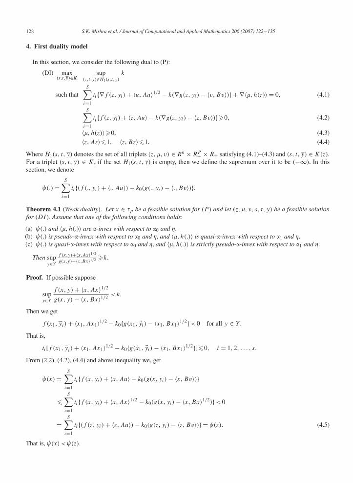
4. First duality model
In this section, we consider the following dual to (P):
(DI) max(s,t,y)∈K
sup(z,t,y)∈H1(s,t,y)
k
such thatS∑
i=1
ti{∇f (z, yi) + 〈u, Au〉1/2 − k(∇g(z, yi) − 〈v, Bv〉)} + ∇〈�, h(z)〉 = 0, (4.1)
S∑i=1
ti{f (z, yi) + 〈z, Au〉 − k(∇g(z, yi) − 〈z, Bv〉)}�0, (4.2)
〈�, h(z)〉�0, (4.3)
〈z, Az〉�1, 〈z, Bz〉�1. (4.4)
Where H1(s, t, y) denotes the set of all triplets (z, �, v) ∈ Rn × RP+ × R+ satisfying (4.1)–(4.3) and (s, t, y) ∈ K(z).For a triplet (s, t, y) ∈ K , if the set H1(s, t, y) is empty, then we define the supremum over it to be (−∞). In thissection, we denote
(.) =S∑
i=1
ti{(f (., yi) + 〈., Au〉) − k0(g(., yi) − 〈., Bv〉)}.
Theorem 4.1 (Weak duality). Let x ∈ �p be a feasible solution for (P ) and let (z, �, v, s, t, y) be a feasible solutionfor (DI). Assume that one of the following conditions holds:
(a) (.) and 〈�, h(.)〉 are �-invex with respect to �0 and �.(b) (.) is pseudo-�-invex with respect to �0 and �, and 〈�, h(.)〉 is quasi-�-invex with respect to �1 and �.(c) (.) is quasi-�-invex with respect to �0 and �, and 〈�, h(.)〉 is strictly pseudo-�-invex with respect to �1 and �.
Then supy∈Y
f (x,y)+〈x,Ax〉1/2
g(x,y)−〈x,Bx〉1/2 �k.
Proof. If possible suppose
supy∈Y
f (x, y) + 〈x, Ax〉1/2
g(x, y) − 〈x, Bx〉1/2 < k.
Then we get
f (x1, yi) + 〈x1, Ax1〉1/2 − k0{g(x1, �yi) − 〈x1, Bx1〉1/2} < 0 for all y ∈ Y .
That is,
ti[f (x1, yi) + 〈x1, Ax1〉1/2 − k0{g(x1, �yi) − 〈x1, Bx1〉1/2}]�0, i = 1, 2, . . . , s.
From (2.2), (4.2), (4.4) and above inequality we, get
(x) =S∑
i=1
ti{f (x, yi) + 〈x, Au〉 − k0(g(x, yi) − 〈x, Bv〉)}
�S∑
i=1
ti{f (x, yi) + 〈x, Ax〉1/2 − k0(g(x, yi) − 〈x, Bx〉1/2)} < 0
=S∑
i=1
ti{(f (z, yi) + 〈z, Au〉) − k0(g(z, yi) − 〈z, Bv〉)} = (z). (4.5)
That is, (x) < (z).
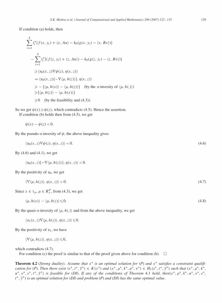
S.K. Mishra et al. / Journal of Computational and Applied Mathematics 206 (2007) 122–135 129
If condition (a) holds, then
S∑i=1
t∗i {f (x, yi) + 〈x, Au〉 − k0(g(x, yi) − 〈x, Bv〉)}
−S∑
i=1
t∗i {(f (z, yi) + 〈z, Au〉) − k0(g(z, yi) − 〈z, Bv〉)}
�〈�0(x, z)∇(z), �(x, z)〉= 〈�0(x, z){−∇〈�, h(z)〉}, �(x, z)〉� − [〈�, h(x)〉 − 〈�, h(z)〉] (by the �-invexity of 〈�, h(.)〉)�[〈�, h(z)〉 − 〈�, h(x)〉]�0 (by the feasibility and (4.3)).
So we get (x)�(z), which contradicts (4.5). Hence the assertion.If condition (b) holds then from (4.5), we get
(x) − (z) < 0.
By the pseudo-�-invexity of , the above inequality gives
〈�0(x, z)∇(z), �(x, z)〉 < 0. (4.6)
By (4.6) and (4.1), we get
〈�0(x, z){−∇〈�, h(z)〉}, �(x, z)〉 < 0.
By the positivity of �0, we get
〈∇〈�, h(z)〉, �(x, z)〉 > 0. (4.7)
Since x ∈ �p, � ∈ RP+ , from (4.3), we get
〈�, h(x)〉 − 〈�, h(z)〉�0. (4.8)
By the quasi-�-invexity of 〈�, h(.)〉 and from the above inequality, we get
〈�1(x, z)∇〈�, h(z)〉, �(x, z)〉�0.
By the positivity of �1, we have
〈∇〈�, h(z)〉, �(x, z)〉�0,
which contradicts (4.7).For condition (c) the proof is similar to that of the proof given above for condition (b). �
Theorem 4.2 (Strong duality). Assume that x∗ is an optimal solution for (P) and x∗ satisfies a constraint qualifi-cation for (P). Then there exist (s∗, t∗, y∗) ∈ K(x∗) and (x∗, �∗, k∗, u∗, v∗) ∈ H1(s
∗, t∗, y∗) such that (x∗, �∗, k∗,u∗, v∗, s∗, t∗, y∗) is feasible for (DI). If any of the conditions of Theorem 4.1 hold, then(x∗, �∗, k∗, u∗, v∗, s∗,t∗, y∗) is an optimal solution for (DI) and problem (P) and (DI) has the same optimal value.
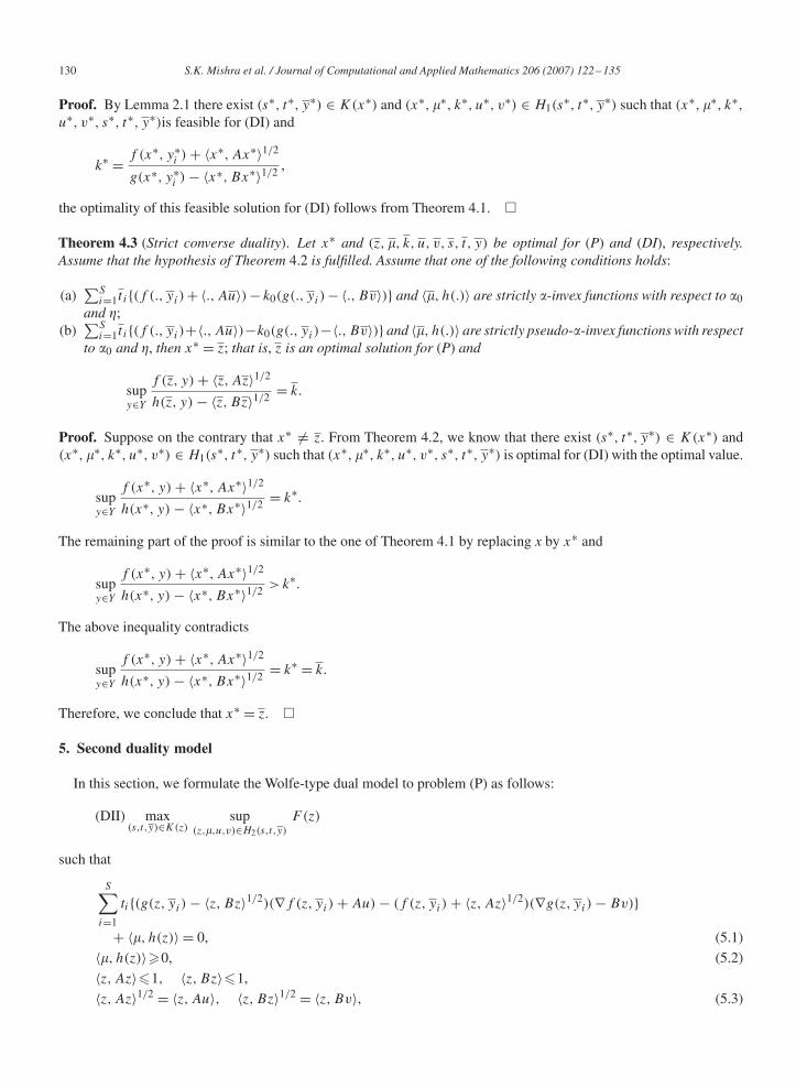
130 S.K. Mishra et al. / Journal of Computational and Applied Mathematics 206 (2007) 122–135
Proof. By Lemma 2.1 there exist (s∗, t∗, y∗) ∈ K(x∗) and (x∗, �∗, k∗, u∗, v∗) ∈ H1(s∗, t∗, y∗) such that (x∗, �∗, k∗,
u∗, v∗, s∗, t∗, y∗)is feasible for (DI) and
k∗ = f (x∗, y∗i ) + 〈x∗, Ax∗〉1/2
g(x∗, y∗i ) − 〈x∗, Bx∗〉1/2 ,
the optimality of this feasible solution for (DI) follows from Theorem 4.1. �
Theorem 4.3 (Strict converse duality). Let x∗ and (z, �, k, u, v, s, t, y) be optimal for (P) and (DI), respectively.Assume that the hypothesis of Theorem 4.2 is fulfilled. Assume that one of the following conditions holds:
(a)∑S
i=1t i{(f (., yi) + 〈., Au〉) − k0(g(., yi) − 〈., Bv〉)} and 〈�, h(.)〉 are strictly �-invex functions with respect to �0and �;
(b)∑S
i=1t i{(f (., yi)+〈., Au〉)−k0(g(., yi)−〈., Bv〉)} and 〈�, h(.)〉 are strictly pseudo-�-invex functions with respectto �0 and �, then x∗ = z; that is, z is an optimal solution for (P) and
supy∈Y
f (z, y) + 〈z, Az〉1/2
h(z, y) − 〈z, Bz〉1/2 = k.
Proof. Suppose on the contrary that x∗ �= z. From Theorem 4.2, we know that there exist (s∗, t∗, y∗) ∈ K(x∗) and(x∗, �∗, k∗, u∗, v∗) ∈ H1(s
∗, t∗, y∗) such that (x∗, �∗, k∗, u∗, v∗, s∗, t∗, y∗) is optimal for (DI) with the optimal value.
supy∈Y
f (x∗, y) + 〈x∗, Ax∗〉1/2
h(x∗, y) − 〈x∗, Bx∗〉1/2 = k∗.
The remaining part of the proof is similar to the one of Theorem 4.1 by replacing x by x∗ and
supy∈Y
f (x∗, y) + 〈x∗, Ax∗〉1/2
h(x∗, y) − 〈x∗, Bx∗〉1/2 > k∗.
The above inequality contradicts
supy∈Y
f (x∗, y) + 〈x∗, Ax∗〉1/2
h(x∗, y) − 〈x∗, Bx∗〉1/2 = k∗ = k.
Therefore, we conclude that x∗ = z. �
5. Second duality model
In this section, we formulate the Wolfe-type dual model to problem (P) as follows:
(DII) max(s,t,y)∈K(z)
sup(z,�,u,v)∈H2(s,t,y)
F (z)
such that
S∑i=1
ti{(g(z, yi) − 〈z, Bz〉1/2)(∇f (z, yi) + Au) − (f (z, yi) + 〈z, Az〉1/2)(∇g(z, yi) − Bv)}
+ 〈�, h(z)〉 = 0, (5.1)
〈�, h(z)〉�0, (5.2)
〈z, Az〉�1, 〈z, Bz〉�1,
〈z, Az〉1/2 = 〈z, Au〉, 〈z, Bz〉1/2 = 〈z, Bv〉, (5.3)

S.K. Mishra et al. / Journal of Computational and Applied Mathematics 206 (2007) 122–135 131
where
F(z) = supy∈Y
[(f (z, y) + 〈z, Az〉1/2)/(h(z, y) − 〈z, Bz〉1/2)],
yi ∈ Y (z) and H2(s, t, y) denotes the set of (z, �, u, v) ∈ Rn × RP+ × Rn × Rn satisfying (5.15), (6.1) and (6.2). If theset H2(s, t, y) is empty, then we define the supremum over it to be (−∞). In this section, we denote
1(.) =S∑
i=1
ti{(g(z, yi) − 〈z, Bv〉)(f (., yi) + 〈., Au〉) − (f (z, yi) + 〈z, Au〉)(g(., yi) − 〈., Bv〉)}.
Now we establish the following duality theorems between (P) and (DII).
Theorem 5.1 (Weak duality). Let x ∈ �p be a feasible solution for (P) and let (z, �, v, s, t, y) be a feasible solutionfor (DII). Assume that one of the following conditions holds:
(a) 1(.) and 〈�, h(.)〉 are �-invex with respect to �0 and �.(b) 1(.) is pseudo-�-invex with respect to �0 and �, and 〈�, h(.)〉 is quasi-�-invex with respect to �1 and �.(c) 1(.) is quasi-�-invex with respect to �0 and �, and 〈�, h(.)〉 is strictly pseudo-�-invex with respect to �1 and �.
Then
supy∈Y
f (x, y) + 〈x, Ax〉1/2
g(x, y) − 〈x, Bx〉1/2 �F(z).
Proof. On the contrary, if possible suppose for each x ∈ �p,
supy∈Y
f (x, y) + 〈x, Ax〉1/2
g(x, y) − 〈x, Bx〉1/2 < F(z). (5.4)
Since yi ∈ Y (z), i = 1, 2, . . . , s. We have
F(z) = f (z, yi) + 〈z, Az〉1/2
g(z, yi) − 〈z, Bz〉1/2 , i = 1, 2, . . . , s. (5.5)
Following as in [11], we get
1(x) < 1(z). (5.6)
Now if condition (a) holds, we get
1(x) − 1(z)�〈�0(x, z)∇1(z), �(x, z)〉= 〈�0(x, z){−∇〈�, h(z)〉}, �(x, z)〉� − [〈�, h(x)〉 − 〈�, h(z)〉] (by the �-invexity of 〈�, h(.)〉)�[〈�, h(z)〉 − 〈�, h(x)〉]�0 (by the feasibility and (5.2)).
So we get 1(x)�1(z), which contradicts (5.6).If condition (b) holds, assuming
1(x) − 1(z) < 0.
By the pseudo-�-invexity of 1, the above inequality gives
〈�0(x, z)∇1(z), �(x, z)〉 < 0. (5.7)
Now from (5.1) and (5.7), we get
〈�0(x, z){−∇〈�, h(z)〉}, �(x, z)〉 < 0.
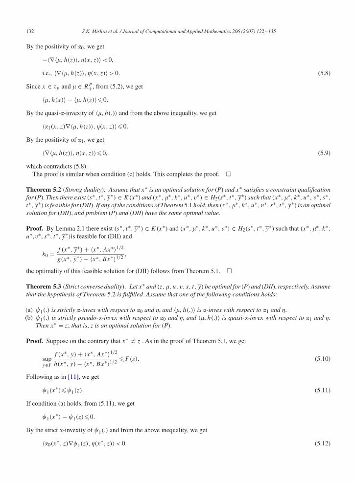
132 S.K. Mishra et al. / Journal of Computational and Applied Mathematics 206 (2007) 122–135
By the positivity of �0, we get
−〈∇〈�, h(z)〉, �(x, z)〉 < 0,
i.e., 〈∇〈�, h(z)〉, �(x, z)〉 > 0. (5.8)
Since x ∈ �p and � ∈ RP+ , from (5.2), we get
〈�, h(x)〉 − 〈�, h(z)〉�0.
By the quasi-�-invexity of 〈�, h(.)〉 and from the above inequality, we get
〈�1(x, z)∇〈�, h(z)〉, �(x, z)〉�0.
By the positivity of �1, we get
〈∇〈�, h(z)〉, �(x, z)〉�0, (5.9)
which contradicts (5.8).The proof is similar when condition (c) holds. This completes the proof. �
Theorem 5.2 (Strong duality). Assume that x∗ is an optimal solution for (P) and x∗ satisfies a constraint qualificationfor (P). Then there exist (s∗, t∗, y∗) ∈ K(x∗) and (x∗, �∗, k∗, u∗, v∗) ∈ H2(s
∗, t∗, y∗) such that (x∗, �∗, k∗, u∗, v∗, s∗,t∗, y∗) is feasible for (DII). If any of the conditions of Theorem 5.1 hold, then (x∗, �∗, k∗, u∗, v∗, s∗, t∗, y∗) is an optimalsolution for (DII), and problem (P) and (DII) have the same optimal value.
Proof. By Lemma 2.1 there exist (s∗, t∗, y∗) ∈ K(x∗) and (x∗, �∗, k∗, u∗, v∗) ∈ H2(s∗, t∗, y∗) such that (x∗, �∗, k∗,
u∗,v∗, s∗, t∗, y∗)is feasible for (DII) and
k0 = f (x∗, y∗) + 〈x∗, Ax∗〉1/2
g(x∗, y∗) − 〈x∗, Bx∗〉1/2 ,
the optimality of this feasible solution for (DII) follows from Theorem 5.1. �
Theorem 5.3 (Strict converse duality). Let x∗ and (z, �, u, v, s, t, y) be optimal for (P) and (DII), respectively. Assumethat the hypothesis of Theorem 5.2 is fulfilled. Assume that one of the following conditions holds:
(a) 1(.) is strictly �-invex with respect to �0 and �, and 〈�, h(.)〉 is �-invex with respect to �1 and �.(b) 1(.) is strictly pseudo-�-invex with respect to �0 and �, and 〈�, h(.)〉 is quasi-�-invex with respect to �1 and �.
Then x∗ = z; that is, z is an optimal solution for (P).
Proof. Suppose on the contrary that x∗ �= z . As in the proof of Theorem 5.1, we get
supy∈Y
f (x∗, y) + 〈x∗, Ax∗〉1/2
h(x∗, y) − 〈x∗, Bx∗〉1/2 �F(z). (5.10)
Following as in [11], we get
1(x∗)�1(z). (5.11)
If condition (a) holds, from (5.11), we get
1(x∗) − 1(z)�0.
By the strict �-invexity of 1(.) and from the above inequality, we get
〈�0(x∗, z)∇1(z), �(x∗, z)〉 < 0. (5.12)

S.K. Mishra et al. / Journal of Computational and Applied Mathematics 206 (2007) 122–135 133
Now from (5.12) and (5.1), we get
〈�0(x∗, z){−∇〈�, h(z)〉}, �(x∗, z)〉 < 0.
By the positivity of �0, we get
−〈∇〈�, h(z)〉, �(x∗, z)〉 < 0.
i.e., 〈∇〈�, h(z)〉, �(x∗, z)〉 > 0. (5.13)
Since x∗ ∈ �p and � ∈ RP+ , from (5.2), we get
〈�, h(x∗)〉 − 〈�, h(z)〉�0.
By the �-invexity of 〈�, h(.)〉 and from the above inequality, we get
〈�1(x∗, z)∇〈�, h(z)〉, �(x∗, z)〉�0.
By the positivity of �1, we get
〈∇〈�, h(z)〉, �(x∗, z)〉�0, (5.14)
which is a contradiction to (5.13).Hence (5.10) is false, so we have
supy∈Y
f (x∗, y) + 〈x∗, Ax∗〉1/2
h(x∗, y) − 〈x∗, Bx∗〉1/2 > F(z). (5.15)
Since x∗ is an optimal solution for (P), from Theorem 5.2 there exist (s∗, t∗, y∗) ∈ K(x∗) and (x∗, �∗, u∗, v∗) ∈H2(s
∗, t∗, y∗) such that (x∗, �∗, u∗, v∗, s∗, t∗, y∗) is an optimal solution for (DII) with the optimal value
supy∈Y
f (x∗, y) + 〈x∗, Ax∗〉1/2
h(x∗, y)〈x∗, Bx∗〉1/2 = F(x∗) = F(z),
which contradicts (5.15). Hence x∗ = z, that is, z is an optimal solution for (P).If condition (b) holds, from (5.11), we get
1(x∗) − 1(z)�0.
By the strict pseudo-�-invexity of 1 and from the above inequality, we get
〈�0(x∗, z)∇1(z), �(x∗, z)〉 < 0.
The remaining part of the proof is similar to that under condition (a). �
6. Third duality model
In this section we take the following form of Lemma 2.1:
Lemma 6.1. Let x∗ be an optimal solution to (P). Assume that ∇gj (x∗), j ∈ J (x∗) are linearly independent. Then
there exist (s∗, t∗, y) ∈ K and �∗ ∈ RP+ such that
∇(∑S∗
i=1t∗i f (x∗, yi) + 〈x∗, Au〉 + 〈�∗, h(x∗)〉∑S∗
i=1t∗i (g(x∗, yi) − 〈x∗, Bv〉)
)= 0, (6.1)
〈�∗, h(x∗)〉 = 0, (6.2)
〈u, Au〉�1, 〈v, Bv〉�1,

134 S.K. Mishra et al. / Journal of Computational and Applied Mathematics 206 (2007) 122–135
〈x∗, Ax∗〉1/2 = 〈x∗, Au〉, 〈x∗, Bx∗〉1/2 = 〈x∗, Bv〉, (6.3)
�∗ ∈ Rp+, t∗i �0,
S∑i=1
t∗i = 1, yi ∈ Y (x∗) where i = 1, 2, . . . , s∗. (6.4)
In this section, we consider the following parameter-free dual problem for (P):
(DIII) max(s,t,y)∈K(z)
sup(z,�,u,v)∈H3(s,t,y)
(∑S∗i=1t
∗i f (z, yi) + 〈z, Au〉 + 〈�, h(z)〉∑S∗i=1t
∗i (g(z, yi) − 〈z, Bv〉)
)
such that ∇(∑S∗
i=1t∗i f (z, yi) + 〈z, Au〉 + 〈�, h(z)〉∑S∗i=1t
∗i (g(z, yi) − 〈z, Bv〉)
)= 0, (6.5)
〈u, Au〉�1, 〈v, Bv〉�1,
〈z, Az〉1/2 = 〈z, Au〉, 〈z, Bz〉1/2 = 〈z, Bv〉, (6.6)
where H3(s, t, y) denotes the set of (z, �, u, v) ∈ Rn × RP+ × Rn × Rn satisfying (6.5). If the set H3(s, t, y) is empty,then we define the supremum over it to be (−∞). Throughout this section for the sake of simplicity, we denote by2(.),
[t∗i {g(z, yi) − 〈z, Bv〉}]⎛⎝ S∑
i=1
tif (., yi) +P∑
j=1
�j gj (.)
⎞⎠
−(
S∑i=1
t∗i {f (z, yi) + 〈z, Au〉} + 〈�, h(z)〉)
[t∗i {g(., yi) − 〈., Bv〉}].
Now we shall state weak, strong and converse duality theorems without proof as they can be proved in light ofTheorems 5.1 and 5.2, proved in previous section.
Theorem 6.1 (Weak duality). Let x ∈ �p be a feasible solution for (P) and let (z, �, u, v, s, t, y) be a feasible solutionfor (DIII). If 2(.) is pseudo-�-invex with respect to �0 and �, then
supy∈Y
f (x, y) + 〈x, Ax〉1/2
g(x, y) − 〈x, Bx〉1/2 �(∑S∗
i=1tif (z, yi) + 〈z, Au〉 + 〈�, h(z)〉∑S∗i=1ti (g(z, yi) − 〈z, Bv〉)
).
Theorem 6.2 (Strong duality). Let x∗ be an optimal solution for (P). Satisfying the hypothesis of Theorem 6.1. Thenthere exist (s∗, t∗, y∗) ∈ K(x∗) and (x∗, �∗, u∗, v∗) ∈ H2(s
∗, t∗, y∗) such that (x∗, �∗, u∗, v∗, s∗, t∗, y∗) is feasiblefor (DIII). If any of the conditions of Theorem 6.1 hold, then (x∗, �∗, u∗, v∗, s∗, t∗, y∗) is an optimal solution for (DIII)and problem (P) and (DIII) has the same optimal value.
Theorem 6.3 (Strict converse duality). Assume that x∗ is an optimal solution for (P) and let (z, �, u, v, s, t, y) be anoptimal solution for (DIII). Assume that the hypothesis of Theorem 6.2 is fulfilled and 2(.) is strictly pseudo-�-invexwith respect to �0 and �, then z = x∗ is an optimal solution of (P).
Acknowledgements
The authors are thankful to the referees for their valuable suggestions for the improvement of the paper.
References
[1] C.R. Bector, B.L. Bhatia, Sufficient optimality and duality for a minimax problem, Utilitas Math. 27 (1985) 229–247.[2] C.R. Bector, S. Chandra, I. Husain, Second order duality for a minimax programming problem, Opsearch 28 (1991) 249–263.[3] C.R. Bector, S. Chandra, V. Kumar, Duality for minimax programming involving V -invex functions, Optimization 30 (1994) 93–103.

S.K. Mishra et al. / Journal of Computational and Applied Mathematics 206 (2007) 122–135 135
[4] C.R. Bector, S.K. Suneja, S. Gupta, Univex functions and univex nonlinear programming, Proceedings of theAdministrative SciencesAssociationof Canada, 1992, pp.115–124.
[5] S. Chandra, V. Kumar, Duality in fractional minimax programming, J. Austral. Math. Soc. Ser. A 58 (1995) 376–386.[6] M.A. Hanson, On sufficiency of the Kuhn–Tucker conditions, J. Math. Anal. Appl. 80 (1981) 545–550.[7] M.A. Hanson, B. Mond, Further generalization of convexity on mathematical programming, J. Inform. Optim. Sci. 3 (1982) 25–32.[8] M.A. Hanson, R. Pini, C. Singh, Multiobjective programming under generalized type-I invexity, J. Math. Anal. Appl. 261 (2001) 562–577.[9] V. Jeyakumar, B. Mond, On generalized convex mathematical programming, J. Austral. Math. Soc. Ser. B 34 (1992) 43–53.
[10] R.N. Kaul, S.K. Suneja, M.K. Srivastava, Optimality criteria and duality in multiple objective optimization involving generalized invexity, J.Optim. Theory Appl. 80 (1994) 465–482.
[11] H.C. Lai, J.C. Lee, On duality theorems for a nondifferentiable minimax fractional programming, J. Comput. Appl. Math. 146 (2002)115–126.
[12] H.C. Lai, J.C. Liu, K. Tanaka, Necessary & sufficient conditions for minimax fractional programming, J. Math. Anal. Appl. 230 (1999)311–328.
[13] J.C. Liu, C.S. Wu, R.L. Sheu, On minimax fractional optimality conditions with invexity, J. Math. Anal. Appl. 219 (1998) 21–35.[14] S.K. Mishra, Pseudolinear fractional minimax programming, Indian J. Pure Appl. Math. 26 (8) (1995) 722–763.[15] S.K. Mishra, Generalized fractional programming problems containing locally sub differentiable �-univex functions, Optimization 41 (1997)
135–158.[16] S.K. Mishra, Generalized pseudoconvex minimax programming, Opsearch 35 (1998) 32–44.[17] S.K. Mishra, Pseudoconvex complex minimax programming, Indian J. Pure Appl. Math. 32 (2) (2001) 205–213.[18] S.K. Mishra, Complex minimax programming under generalized type-I functions, Comput. Math. Appl. 50 (2005) 1–11.[19] S.K. Mishra, G. Giorgi, S.Y. Wang, Duality in vector optimization in banach spaces with generalized convexity, J. Global Optim. 29 (2004)
415–424.[20] S.K. Mishra, M.A. Noor, On vector variational-like inequality problems, J. Math. Anal. Appl. 311 (2005) 69–75.[21] S.K. Mishra, S.Y. Wang, K.K. Lai, Complex minimax programming under generalized convexity, J. Comput. Appl. Math. 167 (2004) 59–71.[22] S.K. Mishra, S.Y. Wang, K.K. Lai, Optimality and duality in nondifferentiable and multiobjective programming under generalized d-invexity,
J. Global Optim. 29 (2004) 425–438.[23] S.K. Mishra, S.Y. Wang, K.K. Lai, Optimality and duality for multiple objective optimization under generalized type-I univexity, J. Math. Anal.
Appl. 303 (2005) 315–326.[24] S.K. Mishra, S.Y. Wang, K.K. Lai, Multiple objective fractional programming involving semilocally type-I preinvex and related functions, J.
Math. Anal. Appl. 310 (2005) 626–640.[25] M.A. Noor, On generalized preinvex functions and monotonicities, J. Inequalities Pure Appl. Math. 5 (2004) 1–9.[26] W.E. Schmitendorf, Necessary conditions and sufficient conditions for static minimax problems, J. Math. Anal. Appl. 57 (1977) 683–693.[27] T. Weir, Pseudoconvex minimax programming, Utilitas Math. 42 (1992) 234–240.[28] S.R. Yadav, R.N. Mukherjee, Duality for fractional minimax programming problems, J. Austral. Math. Soc. Ser. B 31 (1990) 484–492.[29] G.J. Zalmai, Optimality criteria and duality for a class of minimax programming problems with generalized invexity conditions, Utilitas Math.
32 (1987) 35–57.