generalized estimating equations (gee) for...
TRANSCRIPT

Generalized Estimating Equations (gee)for glm–type data
Søren Højsgaard
mailto:[email protected]
Biometry Research Unit
Danish Institute of Agricultural Sciences
January 23, 2006
Printed: January 23, 2006 File: R-mixed-geeglm-Lecture.tex
2
Contents1 Preliminaries 3
2 Working example – respiratory illness 4
3 Correlated Pearson–residuals 9
4 Marginal vs. conditional models 12
5 Marginal models for glm–type data 14
6 Estimating equations for gee–type data 166.1 Specifications needed for GEEs . . . . . . . . . . . . . . . . . . . . . . . . . 186.2 Deriving and solving GEEs . . . . . . . . . . . . . . . . . . . . . . . . . . . . 206.3 Newton–iteration . . . . . . . . . . . . . . . . . . . . . . . . . . . . . . . . . 276.4 Estimation of the covariance of β̂ . . . . . . . . . . . . . . . . . . . . . . . . 29
6.4.1 Model based estimate . . . . . . . . . . . . . . . . . . . . . . . . . . 296.4.2 Emperical estimate – sandwich estimate . . . . . . . . . . . . . . . . 30
6.5 The working correlation matrix . . . . . . . . . . . . . . . . . . . . . . . . . 31
7 Exploring different working correlations 33
8 Comparison of the parameter estimates 378.1 When do GEEs work? . . . . . . . . . . . . . . . . . . . . . . . . . . . . . . 398.2 What to do – geeglm vs. lmer . . . . . . . . . . . . . . . . . . . . . . . . . . 40
January 23, 2006 page 2

3
1 Preliminaries
These notes deal with fitting models for responses of type often
dealt with with generalized linear models (glm) but with the
complicating aspect that there may be repeated measurements
on the same unit.
The approach here is generalized estimating equations (gee).
There are two packages for this purpose in R: geepack and gee.
We focus on the former and note in passing that the latter does
not seem to undergo any further development.
The geepack package is described in the paper by Halekoh,
Højsgaard and Yun in Journal of Statistical Software,
www.jstatsoft.org, January 2006.
January 23, 2006 page 3
4
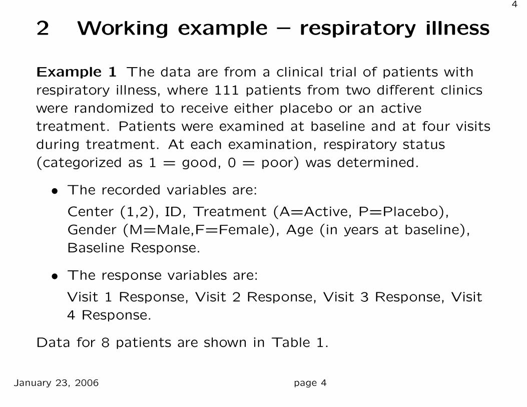
2 Working example – respiratory illness
Example 1 The data are from a clinical trial of patients withrespiratory illness, where 111 patients from two different clinicswere randomized to receive either placebo or an activetreatment. Patients were examined at baseline and at four visitsduring treatment. At each examination, respiratory status(categorized as 1 = good, 0 = poor) was determined.
• The recorded variables are:
Center (1,2), ID, Treatment (A=Active, P=Placebo),Gender (M=Male,F=Female), Age (in years at baseline),Baseline Response.
• The response variables are:
Visit 1 Response, Visit 2 Response, Visit 3 Response, Visit4 Response.
Data for 8 patients are shown in Table 1.
January 23, 2006 page 4

5
center id treat sex age baseline visit1 visit2 visit3 visit4
1 1 1 P M 46 0 0 0 0 0
2 1 2 P M 28 0 0 0 0 0
3 1 3 A M 23 1 1 1 1 1
4 1 4 P M 44 1 1 1 1 0
5 1 5 P F 13 1 1 1 1 1
6 1 6 A M 34 0 0 0 0 0
7 1 7 P M 43 0 1 0 1 1
8 1 8 A M 28 0 0 0 0 0
Table 1: Respiratory data for eight individuals. Measurements on
the same individual tend to be alike.
January 23, 2006 page 5

6
Interest is in comparing the treatments, but also to includecenter, age, gender and baseline response in the model.
From Table 1 it is clear, that there is a dependency among theresponse measurements on the same person – measurements onthe same person tend to be alike.
This dependency must be accounted for in the modelling. �
January 23, 2006 page 6
7
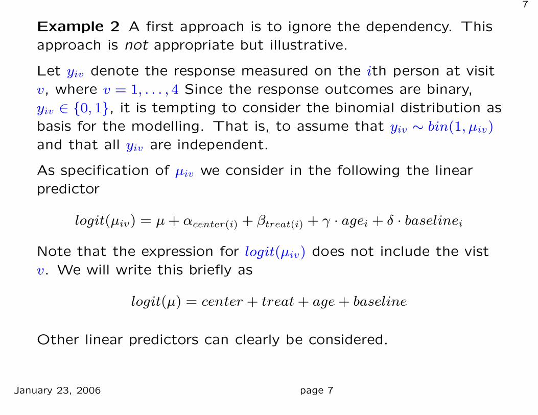
Example 2 A first approach is to ignore the dependency. Thisapproach is not appropriate but illustrative.
Let yiv denote the response measured on the ith person at visitv, where v = 1, . . . , 4 Since the response outcomes are binary,yiv ∈ {0, 1}, it is tempting to consider the binomial distribution asbasis for the modelling. That is, to assume that yiv ∼ bin(1, µiv)
and that all yiv are independent.
As specification of µiv we consider in the following the linearpredictor
logit(µiv) = µ+ αcenter(i) + βtreat(i) + γ · agei + δ · baselinei
Note that the expression for logit(µiv) does not include the vistv. We will write this briefly as
logit(µ) = center + treat+ age+ baseline
Other linear predictors can clearly be considered.
January 23, 2006 page 7

8
Table 2 contains the parameter estimates under the model.
Estimate Std. Error z value Pr(>|z|)
(Intercept) −0.20 0.52 −0.39 0.70
center 1.07 0.22 4.94 0.00
sexM 0.11 0.27 0.41 0.68
age −0.02 0.01 −2.62 0.01
treatP −1.01 0.21 −4.79 0.00
Table 2: Parameter estimates when assuming independence
A more elaborate model is to allow for over/underdispersion.That is, to make a quasi likelihood model where the variancefunction is
φµiv(1− µiv)
The dispersion parameter φ is estimated as φ̂ = 1.009, i.e. thereis no indication of over/under dispersion. �
January 23, 2006 page 8
9
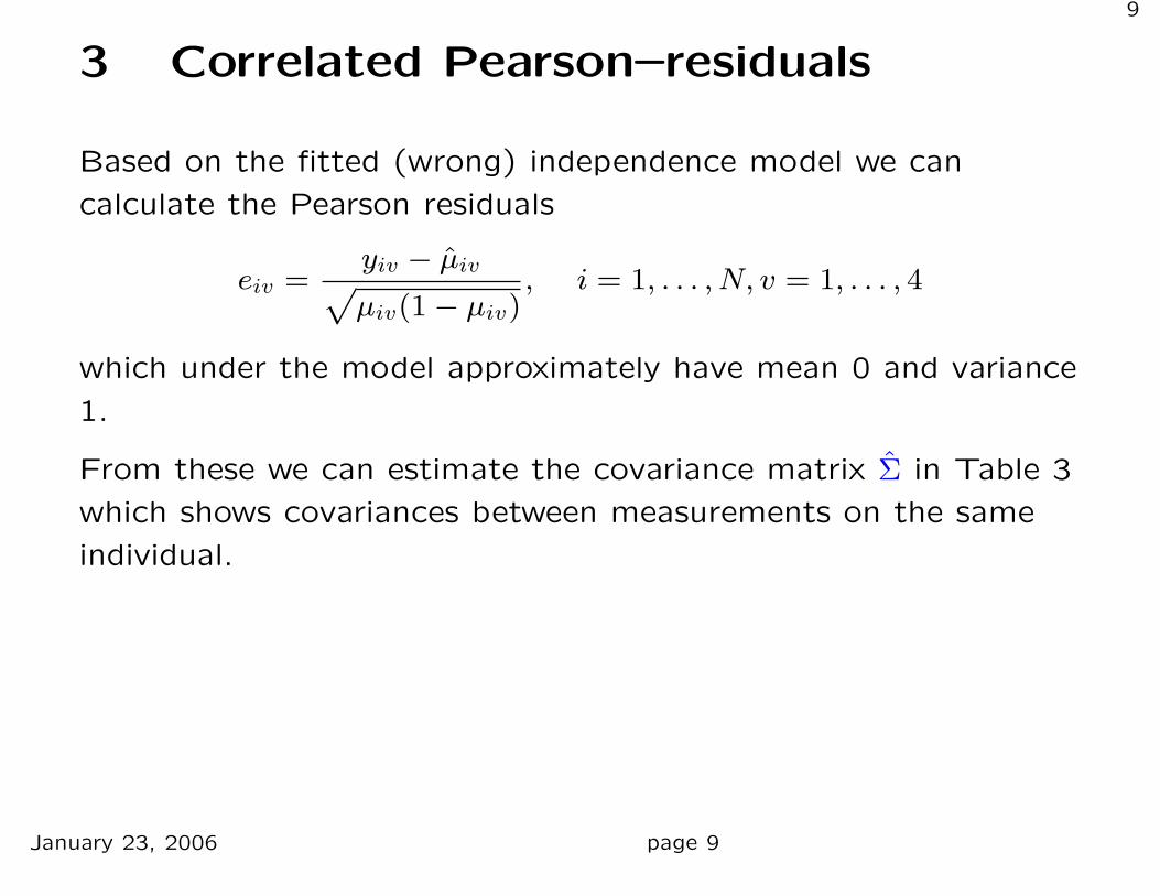
3 Correlated Pearson–residuals
Based on the fitted (wrong) independence model we can
calculate the Pearson residuals
eiv =yiv − µ̂ivpµiv(1− µiv)
, i = 1, . . . , N, v = 1, . . . , 4
which under the model approximately have mean 0 and variance
1.
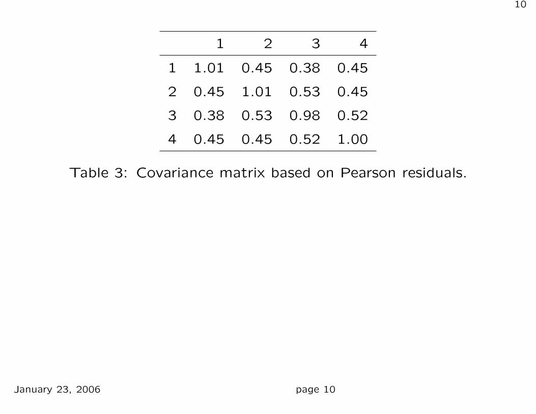
From these we can estimate the covariance matrix Σ̂ in Table 3
which shows covariances between measurements on the same
individual.
January 23, 2006 page 9
10
1 2 3 4
1 1.01 0.45 0.38 0.45
2 0.45 1.01 0.53 0.45
3 0.38 0.53 0.98 0.52
4 0.45 0.45 0.52 1.00
Table 3: Covariance matrix based on Pearson residuals.
January 23, 2006 page 10

11
Since the elements on the diagonal in Table 3 are about 1, the
matrix can also be regarded as a correlation matrix.
If the observations were independent then the true (i.e.
theoretical) correlations should be zero.
The estimated correlations in Table 3 suggest that there is a
positive correlation.
The task in the following is to account for the correlation
between measurements on the same individual.
January 23, 2006 page 11
12
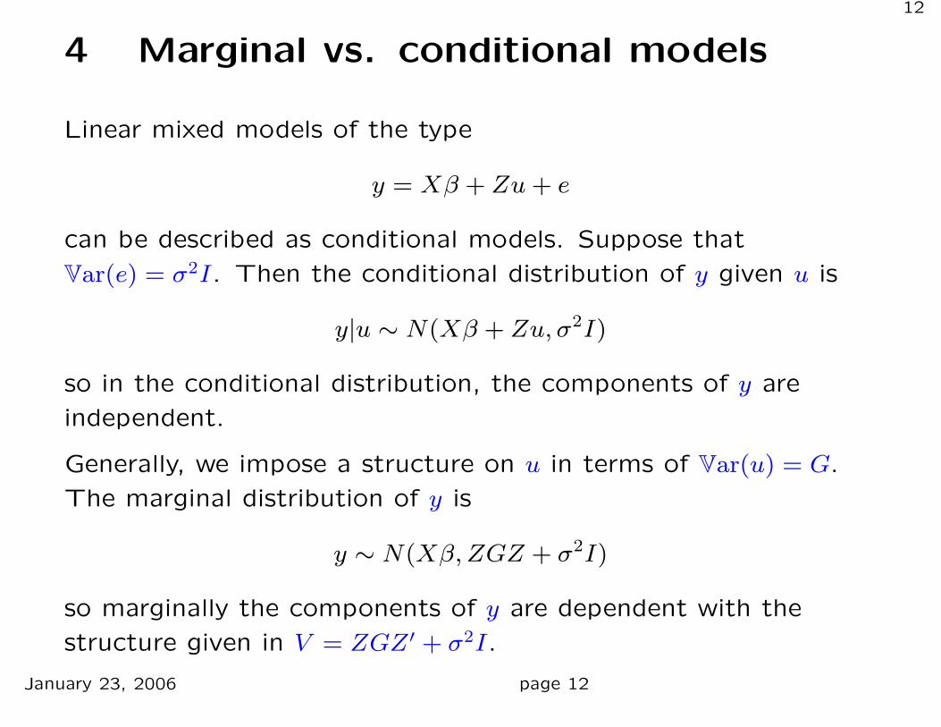
4 Marginal vs. conditional models
Linear mixed models of the type
y = Xβ + Zu+ e
can be described as conditional models. Suppose that
Var(e) = σ2I. Then the conditional distribution of y given u is
y|u ∼ N(Xβ + Zu, σ2I)
so in the conditional distribution, the components of y are
independent.
Generally, we impose a structure on u in terms of Var(u) = G.
The marginal distribution of y is
y ∼ N(Xβ,ZGZ + σ2I)
so marginally the components of y are dependent with the
structure given in V = ZGZ ′ + σ2I.
January 23, 2006 page 12

13
So this way, one can see the linear mixed model formula as a way
of building up a model in which the responses are correlated.
An alternative approach is to construct a marginal model
directly, e.g.
y ∼ N(Xβ, V )
by specifying directly a structure on V .
January 23, 2006 page 13

14
5 Marginal models for glm–type data
A way of dealing with correlated glm–type observations is to
create a “marginal model” directly. That is, to create a model
for e.g. a 4–dimensional response vector which consist of binary
variables.
We follow the approach by Liang and Zeger (1986).
The term “marginal model” is quoted, because formally we do
not specify a proper statistical model (in terms of making
distributional assumptions).
All we do is to to specify
1. how the mean E(y) depends on the covariates through a link
function g(E(y)) = Xβ and
2. how the variance Var(y) varies as a function of the mean
(the variance function), i.e. Var(y) = v(E(y)).
January 23, 2006 page 14

15
With these specifications, one can derive a system of estimating
equations by which an estimate β̂ and Var(β̂) can be obtained.
Asymptotically β̂ ∼ N(β, ...).
So we make fewer assumptions than if we specify a full
statistical model. This extra flexibility comes at a price:
• The estimate β̂ may not be the best possible.
• Hypothesis testing is based on Wald tests (since, as there is
no distribution and hence no likelihood).
• Model checking is difficult.
One can regard GEEs as a “quick and dirty” method.
January 23, 2006 page 15

16
6 Estimating equations for gee–type
data
For correlated glm–type data, estimating equations have in the
litterature become known as generalised estimating equations
(GEEs).
• GEEs can, in connection with correlated glm–type data, be
regarded as an extension of the esimation methods (score
equations) used GLMs/QLs. This justifies the term
“generalized”.
• On the other hand, the estimating equations used in
connection with correlated glm–type data are are rather
specialized type of estimating equations. As such, the term
“generalized” is a little misleading.
For this reason the function for dealing with these types of data
in the geepack package is called geeglm().
January 23, 2006 page 16
17
With GEEs for GLM–type data
• the emphasis is on modeling the expectation of the
dependent variable in relation to the covariates (just like
with GLMs), whereas
• the correlation structure is considered to be a nuisance (not
of interest in itself), which is accounted for by the method.
January 23, 2006 page 17

18
6.1 Specifications needed for GEEs
The setting is as follows: On each of i = 1, . . . , N subjects, there
are made ni measurements yi = (yi1, . . . , yini).
• Measurements on different subjects are assumed to be
independent
• Measurements on the same subject are allowed to be
correlated.
The model formulation is similar to that of a GLM:
Systematic part: Relate the expectation E(yit) = µit to the
linear predictor via the link function
h(µit) = ηit = x′itβ
Random part: Specify how the variance Var(yit) is related to
the mean E(yit) by specifying a variance function V (µit)
such that Var(yit) = φV (µit).
January 23, 2006 page 18

19
The correlation part: In addition to these “GLM” steps we
need to impose a correlation structure for observations on
the same unit. This is done by specifying a
working correlation matrix.
January 23, 2006 page 19

20
6.2 Deriving and solving GEEs
Consider observations y1, . . . , yn with common mean θ. The least
squares criterion for estimating µ is to minimize
Ψ(θ, y) =Xi
(yi − θ)2
This is achieved by setting the derivative to zero:
ψ(θ; y) = Ψ′(θ; y) = 2Xi
(yi − θ) = 0
We say that ψ(θ) = ψ(θ; y) is an estimating function and
ψ(θ; y) = 0 is an estimating equation.
January 23, 2006 page 20

21
Consider data y = (y1, . . . , yn) and a model p(y; θ) where
θ ∈ Θ ⊆ Rp. The idea behind estimating functions is to find a
function ψ(θ) which immitates the score function
U(θ) =d
dθlog p(y; θ).
Let
ψ(θ) = ψ(θ, y)
be such a function denoted an estimating function. Solve
(usually by iteration) the estimating equations
ψ(θ) = 0 giving θ̂ = θ̂(y)
If Eθ(ψ(θ)) = 0 for all θ (which holds for the score function), then
ψ is said to be unbiased. (Note that unbiasedness is a property
of the estimation function rather than of the estimate θ̂.)
January 23, 2006 page 21

22
In practice we frequently we consider weighted sums of
estimating functions of the formXi
ai(yi − µi(θ))
which consequently is unbiased.
January 23, 2006 page 22
23
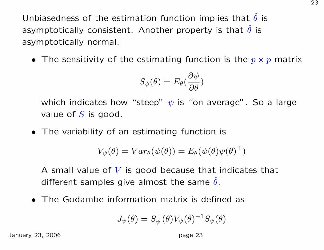
Unbiasedness of the estimation function implies that θ̂ is
asymptotically consistent. Another property is that θ̂ is
asymptotically normal.
• The sensitivity of the estimating function is the p× p matrix
Sψ(θ) = Eθ(∂ψ
∂θ)
which indicates how “steep” ψ is “on average”. So a large
value of S is good.
• The variability of an estimating function is
Vψ(θ) = V arθ(ψ(θ)) = Eθ(ψ(θ)ψ(θ)>)
A small value of V is good because that indicates that
different samples give almost the same θ̂.
• The Godambe information matrix is defined as
Jψ(θ) = S>ψ (θ)Vψ(θ)−1Sψ(θ)
January 23, 2006 page 23

24
• It then holds that
θ̂ ∼approx N(θ, Jψ(θ)−1)
Note: If ψ is the score function (arising from a likelihood) then
Sψ(θ) = −I(θ) and Vψ(θ) = I(θ) and hence Jψ(θ) = I(θ).
If ψ(θ) has the form ψ = X>(y − µ) then
Sψ(θ) = X>[∂µ
∂θ1: · · · :
∂µ
∂θp].
Moreover,
Vψ(θ) = E(ψ(θ))2 = E(X>(y − µ)(y − µ)>X)
which is not so easy to calculate. In principle, however, this
quantity can be estimated using
V̂ψ(θ) = X>(y − µ̂)(y − µ̂)>X
In practice, this may cause problem since V̂ψ in this case may
not be invertible.
January 23, 2006 page 24

25
The GEE by Liang and Zeeger (1986) for estimating a p vector
β is given by
ψ(β) =Xi
∂µ′i∂β
Σ−1i (yi − µi(β)) (1)
Since g(µij) = x′ijβ, the deriavative ∂µ′i
∂βhas as its kjth entry
[∂µ′i∂β
]kj =xikj
g′(µik)
The variance is
Σi = φA1/2i R(α)A
1/2i
where Ai is diagonal with the v(µij)s on the diagonal and R(α) is
the correlation matrix.
The correlation matrix is generally unknown, so therefore one
specifies a “working correlation matrix”, e.g. with an
autoregressive in a repeated measurements problem.
In absence of a good guess of R(α) the identity matrix is often a
good choice.January 23, 2006 page 25

26
Typically R(α) is estimated from data iteratively by using the
current estimate of β to calculate a function of the Pearson
residuals
eij =yij − µij(β)pv(µij(β))
(2)
The dispersion parameter is often estimated as
φ̂ =1
N − p
NXi=1
niXj=1
e2ij (3)
January 23, 2006 page 26

27
6.3 Newton–iteration
The fitting algorithm then becomes
1. Compute an initial estimate of β from a glm (i.e. by
assuming independence)
2. Compute an estimate R(α) of the working correlation on
the basis of the current Pearson residuals and the current
estimate of β
3. Compute an estimate of the variance as
Σi = φA1/2i R̂(α)A
1/2i
4. Compute an updated estimate of β based on the
Newton–step
β := β + [Xi
∂µ′i∂β
Σ−1i
∂µi
∂β′]−1[
Xi
∂µ′i∂β
Σ−1i (yi − µi(β))]
January 23, 2006 page 27
28
Iterate through 2–4 until convergence. Note that φ needs not to
be estimated until the last iteration.
The GEE estimate β̂ of β is often very similar to the estimate
obtained if observations were treated as being independent. In
other words, the estimate β̂ for GEEs is often very similar to the
estimate obtained by fitting a QL–model to the data.
January 23, 2006 page 28

29
6.4 Estimation of the covariance of β̂
There are two classical ways of estimating the covariance Cov(β̂).
6.4.1 Model based estimate
Cov(β̂)m = I−10 , I0 =
Xi
∂µ′i∂β
Σ−1i
∂µi
∂β′
This is the “GEE–version” of inverse Fisher information used
when esitmating Cov(β) in a glm. Here Cov(β̂)m consistently
estimates Cov(β̂) if i) the mean model and ii) the working
correlation are correct.
January 23, 2006 page 29

30
6.4.2 Emperical estimate – sandwich estimate
Cov(β̂)e = I−10 I1I
−10
where
I1 =Xi
∂µ′i∂β
Σ−1i Cov(yi)Σ
−1i
∂µi
∂β′
Here Cov(β̂)e is a consistent estimate of Cov(β̂) even if the
working correlation is misspecified, i.e. if Cov(yi) 6= Σi.
In practice, Cov(yi) is replaced by (yi − µi(β))(yi − µi(β))′.
January 23, 2006 page 30

31
6.5 The working correlation matrix
The notion of working correlation matrices can be introduced
through Example 1 on the respiratory data.
Recall that the measurements on the ith person are
yi = (yi1, . . . , yi4).
It is natural do imagine that the correlation between two
measurements on the same unit decrease as the time between
the measurements increase. A particular simple way of
modelling this as
Corr(yit, yik) = α|t−k|
If |α| < 1 then α|t−k| tends to 0 as |t− k| increase which is what
we wanted. This correlation structure is called an autoregression
of order 1, briefly written ar(1).
January 23, 2006 page 31

32
The ar(1) correlation structure can be written in matrix form as
a correlation matrix:
R(α) =
26666641 α1 α2 α3
α1 1 α1 α2
α2 α1 1 α1
α3 α2 α1 1
3777775Note that R depends on a single unknown parameter α which
must be estimated from data.
Some additional classical working correlation matrices are
presented in Section 7.
January 23, 2006 page 32

33
7 Exploring different working
correlations
Example 3 With the autoregressive working correlationstructure the correlation parameter is estimated as α̂ = 0.61
which implies that the correlation matrix is
1 2 3 4
1 1.00 0.61 0.37 0.23
2 0.61 1.00 0.61 0.37
3 0.37 0.61 1.00 0.61
4 0.23 0.37 0.61 1.00
It is noted that this correlation matrix does not fit very closelyto the empirical matrix in Table 3. �
January 23, 2006 page 33

34
Example 4 Table 3 actually suggests that the correlation isabout the same no matter how far apart the measurements arein time. This corresponds to the exchangable workingcorrelation matrix given by
R(α) =
26666641 α α α
α 1 α α
α α 1 α
α α α 1
3777775(Exchangable means that one can swap the order of any twomeasurements without changing the correlation structure).
The estimated value for α is now α̂ = 0.46 which fits much closerto the empirical matrix in Table 3. �
January 23, 2006 page 34

35
Example 5 The unstructured working correlation matrix is:
R(α) =
26666641 α12 α13 α14
α12 1 α23 α24
α13 α23 1 α34
α14 α24 α34 1
3777775The ustructured working correlation matrix should be used onlywith great care: If there are n measurements per unit there aren(n+ 1)/2 parameters to estimate. This number becomes verylarge even for moderate n. In practice this means that thecorrelation parameters can be poorly estimated or that thestatistical program fails to produce a result. �
January 23, 2006 page 35

36
Example 6 The independence working correlation matrix isparticularly simple:
R =
26666641 0 0 0
0 1 0 0
0 0 1 0
0 0 0 1
3777775With the indpendence working correlation matrix, the actualdependence between the observations is incorporated in themodel only through the emperical covariance (which informallycan be thought of as Table 3).
Note that R does not depend on any unknown parameter.
In absence of important prior knowledge, the independenceworking correlation is often a good choice. �
January 23, 2006 page 36

37
8 Comparison of the parameter
estimates
So far, five models have been considered: 1) observations are
assumed independent 2) a ar(1) working correlation 3) an
exchangable correlation 4) the unstructured working correlation
and 5) the independence working correlation.
Table 4 shows the parameter estimates/ standard errors.
The following general results are illustrated from this table
• The independence and exchangable working correlation
structures produce exactly the same parameter estimates as
one obtains if a GLM is fitted to data. That is always true.
• The standard errors produced by the GEEs are all of a
comparable size (they are practically identical). The
standard errors of the GEEs are about 50 % larger than the
GLM standard errors.
January 23, 2006 page 37

38
Est.GLM SE.GLM Est.Ar1 SE.Ar1 Est.Exc SE.Exc
(Intercept) −0.20 0.52 −0.49 0.82 −0.20 0.82
center 1.07 0.22 1.18 0.34 1.07 0.33
sexM 0.11 0.27 0.13 0.42 0.11 0.41
age −0.02 0.01 −0.02 0.01 −0.02 0.01
treatP −1.01 0.21 −0.91 0.33 −1.01 0.32
Est.GLM SE.GLM Est.Un SE.Un Est.Ind SE.Ind
(Intercept) −0.20 0.52 −0.26 0.81 −0.20 0.82
center 1.07 0.22 1.08 0.33 1.07 0.33
sexM 0.11 0.27 0.13 0.41 0.11 0.41
age −0.02 0.01 −0.02 0.01 −0.02 0.01
treatP −1.01 0.21 −0.99 0.32 −1.01 0.32
Table 4: Comparison of parameter estimates.
January 23, 2006 page 38

39
8.1 When do GEEs work?
GEE works best if
• the number of observations per subject is small and the
number of subjects is large
• in longitudinal studies (e.g. growth curves) the
measurements are taken at the same times for all subjects
January 23, 2006 page 39

40
8.2 What to do – geeglm vs. lmer
Consider this example: On several subjects i, a binary response
yit has been measured on t = 1, . . . , 4 occasions. Suppose the
subjects have been given either control or treatment.
Marginal models – geeglm()
• The starting point for a marginal model with geeglm() is to
model the parameter pit = Pr(yit = 1) of interest, e.g.
logit pit = αtreat(i)
• We specify a variance function, e.g. Var(yit) = pit(1− pit).
• Then we specify a corelation structure which should
“capture” that yi1, . . . , yi4 are dependent, e.g. an ar(1)
structure.
• After fitting such a “model” we get a parameter estimate
α̂1, α̂2 together with a variance estimate Var(α̂k).
January 23, 2006 page 40

41
• We do not get a (usable) measure of how “correlated”
measurements on the same unit are.
Conditional models – lmer()
• For a conditional model with lmer(), the starting point is to
assume that yit ∼ bern(pit) and that
logit pit = αtreat(i) + Ui, Ui ∼ N(0, σ2U )
Hence, conditional on Ui, yi1, . . . , yi4 are independent
unconditionally they are not.
• After fitting such a “model” we get a parameter estimate
α̂1, α̂2 together with a variance estimate Var(α̂k) – and an
estimate of σ2U .
• It is not clear how to obtain a (usable) measure of how
“correlated” measurements on the same unit are – at least
not on an interpretable scale.
January 23, 2006 page 41
42
• Moreover, we have
pit =exp(αtreat(i) + Ui)
1 + exp(αtreat(i) + Ui)
and as such, Ui are difficult to interpret.
January 23, 2006 page 42