generalized diagonal band copulas

Insurance: Mathematics and Economics 37 (2005) 49–67

Generalized diagonal band copulas

Daniel Lewandowski∗

Department of Mathematics, Delft University of Technology, Mekelweg 4, 2628 CD Delft, The Netherlands

Received April 2004; received in revised form October 2004; accepted 13 December 2004

Abstract

This paper investigates the class of generalized diagonal band (GDB) copulas, which form an extension of diagonal band (DB)copulas originally introduced by Cooke and Waij [Cooke, R.N., Waij, R., 1986. Monte Carlo sampling for generalized knowledgedependence, with application to human reliability. Risk Anal. 6, 335–343] for application in simulating high-dimensionaldistributions for dependent random variables. Ferguson [Ferguson, T.S., 1995. A class of bivariate uniform distributions. Stat.Pap. 36, 31–40] provided a method for constructing copulas which include the convex closure of DB copulas. Bojarski [Bojarski,J., 2001. A New Class of Band Copulas—Distributions with Uniform Marginals, Technical Publication. Institute of Mathematics,Technical University of Zielona Gora] provided a different extension of the original DB construction and obtained (independently)the same class as Ferguson, which we now call the GDB. Our interest in GDB copulas results from their possible application inthe vine–copula method for simulating high-dimensional dependent vectors; see Cooke [Cooke, R.M., 1997. Markov and entropyproperties of tree- and vine-dependent variables. Proceedings of the ASA Section on Bayesian Statistical Science],Bedford andCooke [Ann. Math. Artif. Intel. 32 (2001) 245–268], andKurowicka and Cooke [Linear Algebra Appl. 372 (2003) 225–251].This method requires using copulas with certain properties which GDB copulas often possess. We list these requirements andconstruct distributions that meet them using the class of GDB copulas.© 2005 Elsevier B.V. All rights reserved.

Keywords:Diagonal band copulas; High-dimensional distribution; Rank correlation

1. Introduction

Copulas represent a natural tool for modeling high-dimensional distributions for Markov-dependence trees anda recent generalization thereof called vines(Bedford and Cooke, 2002)in which a multivariate distribution is builtfrom bivariate pieces with given rank correlations. This methodology has been successfully applied in uncertaintyanalysis combined with expert judgment(Cooke, 1991).

∗ Tel.: +31 15 278 7262; fax: +31 15 278 7255.E-mail address:[email protected].

0167-6687/$ – see front matter © 2005 Elsevier B.V. All rights reserved.doi:10.1016/j.insmatheco.2004.12.006

50 D. Lewandowski / Insurance: Mathematics and Economics 37 (2005) 49–67

Suppose we want to build a multivariate distribution based only on very limited information, such as univariatemarginals and rank correlations elicited from experts. Assuming that these constraints are feasible, it would then benatural to choose that distribution which adds as little information as possible beyond them. The notion of mutualinformation between two continuous random variables can help to make this statement more precise.

Letf (x, y) denote the joint density of a random pair (X, Y ), and denote byfX andfY the corresponding marginals.The amountI(X|Y ) of information that each variable contains about the other may then be defined as

I(X|Y ) =∫∫

f (x, y) log

{f (x, y)

fX(x)fY (y)

}dx dy ≥ 0. (1)

In the special case wherefX andfY are uniform on the interval (0, 1), Eq.(1) represents the relative information of thecopula densityf (x, y) with respect to the independence copulafX(x)fY (y) = 1. More generally,I(X|Y ) vanishesif, and only if, X andY are independent. In view of Theorems 7 and 12 inCooke (1997), the least informativedistribution with given univariate marginals and fixed rank correlation structure is obtained by the least informativecopula that meets the dependence constraints.

Meeuwissen and Bedford (1997)showed that the densityf (x, y) of the minimally informative copula with givenrank correlationρ(θ) is of the form:

fθ(x, y) = κ

(x − 1

2

)κ

(y − 1

2

)eθ(x−1/2)(y−1/2), (2)

whereκ(x − 1/2) is even aroundx = 1/2. The correlation induced by this copula is controlled by the parameterθ. Although a Taylor series expansion for(2) is available, this minimally informative copula is not tractable andmust be numerically approximated for each value ofθ through a discretized optimization problem. An additionaldifficulty associated with the use of(2) is that no analytical form is generally available for its conditional cumulativedistribution functions and their inverses. Accordingly, simulating from the least informative copula is inconvenient.

In this paper, the search for a minimally informative copula satisfying correlation constraints is not consideredin full generality, but rather within the broad class of generalized diagonal band (GDB) copulas introduced byFerguson (1995). This family of copulas, described in Section2, extends the class of diagonal band (DB) copulasfirst considered byCooke and Waij (1986). Those GDB copulas that can be recovered by mixing only DB copulasare characterized in Section3. In Section4, we then deal specifically with the problem of approximating minimallyinformative GDB copulas with given correlation. Section5 contains three examples of GDB copulas generatedusing Ferguson’s method for constructing distributions in the convex closure of DB copulas; two other copulasalready implemented in a software for uncertainty modeling calledunicorn are also described there. These fiveclasses of copulas are then compared in Section6 in terms of their relative information with respect to the uniformbackground measure under given correlation constraint. Finally, Section7 contains conclusions.

2. Construction and properties of the generalized diagonal band copula

Introduced byFerguson (1995), the generalized diagonal band (GDB) copula of a pair (X, Y ) of uniform randomvariables on the unit interval is defined as follows.

Definition 2.1. LetZbe a continuous random variable on the interval [0, 1] with densityg. An absolutely continuouscopulaC is a generalized diagonal band (GDB) copula if its associated density is of the form:

c(x, y) = 1

2{g(|x − y|) + g(1 − |1 − x − y|)}. (3)

In the sequel,g is called the generating density of the GDB copula.

D. Lewandowski / Insurance: Mathematics and Economics 37 (2005) 49–67 51

In his paper,Ferguson (1995)emphasized that each GDB copula may be seen as a mixture of bivariate uniformdensities on the boundaries of rectangles with corners (z, 0), (0, z), (1− z, 1) and (1, 1 − z). The weight of eachof the densities is given byg(z), z ∈ [0, 1]. Most of the basic properties of GDB copulas stem from this fact. Inparticular, note the symmetries:

g(x) = c(x, 0) = c(1 − x, 1) and g(y) = c(0, y) = c(1, 1 − y)

and the fact that for any (x, y) ∈ A = {(x, y)|0 ≤ y ≤ 1/2, y ≤ x ≤ −y + 1}, Eq.(3) simplifies to

c(x, y) = g(x − y) + g(x + y)

2.

For our purposes, one major advantage of the class of GDB copulas is that the mutual information associated withany copula of the form(1) can be expressed in terms of its generating densityg. To see this, first observe that in thelight of the symmetry ofc and the above identity, we have

I(c|u) = 4∫∫A

c(x, y) log{c(x, y)}dx dy,

whereudenotes the uniform density on the unit square. Now if we substitutex + y = v andx − y = t (with Jacobian1/2), we get

I(c|u) =∫ 1

0

∫ v

0{g(v) + g(t)} log{g(v) + g(t)} dt dv −

∫ 1

0

∫ v

0{g(v) + g(t)} log(2) dt dv.

But

∫ 1

0

∫ v

0{g(v) + g(t)} dt dv = 4

∫∫A

g(x − y) + g(x + y)

2dx dy = 1

and hence

I(c|u) =∫ 1

0

∫ v

0{g(v) + g(t)} log{g(v) + g(t)} dt dv − log(2). (4)

A second major advantage of the GDB class of copulas for our purposes stems from the simple relationshipbetween the generating densitygof a GDB copulaCand the value of Spearman’s rho for the associated pair (X, Y ).To be specific,Ferguson (1995)showed that ifZ is distributed asg, then

ρ(X, Y ) = 1 − 6E(Z2) + 4E(Z3). (5)

Using this fact and the above mentioned symmetries, one can thus check that if the GDB copula generated byg(z) has correlationρ, theng(1 − z) generates a GDB copula with correlation−ρ. Furthermore, the followingrelationships between the two GDB copulas hold:

c(x, y; ρ) = c(1 − x, y; −ρ), CY |X=x(y; ρ) = CY |X=1−x(y; −ρ),

C−1Y |X=x(y; ρ) = C−1

Y |X=1−x(y; −ρ). (6)


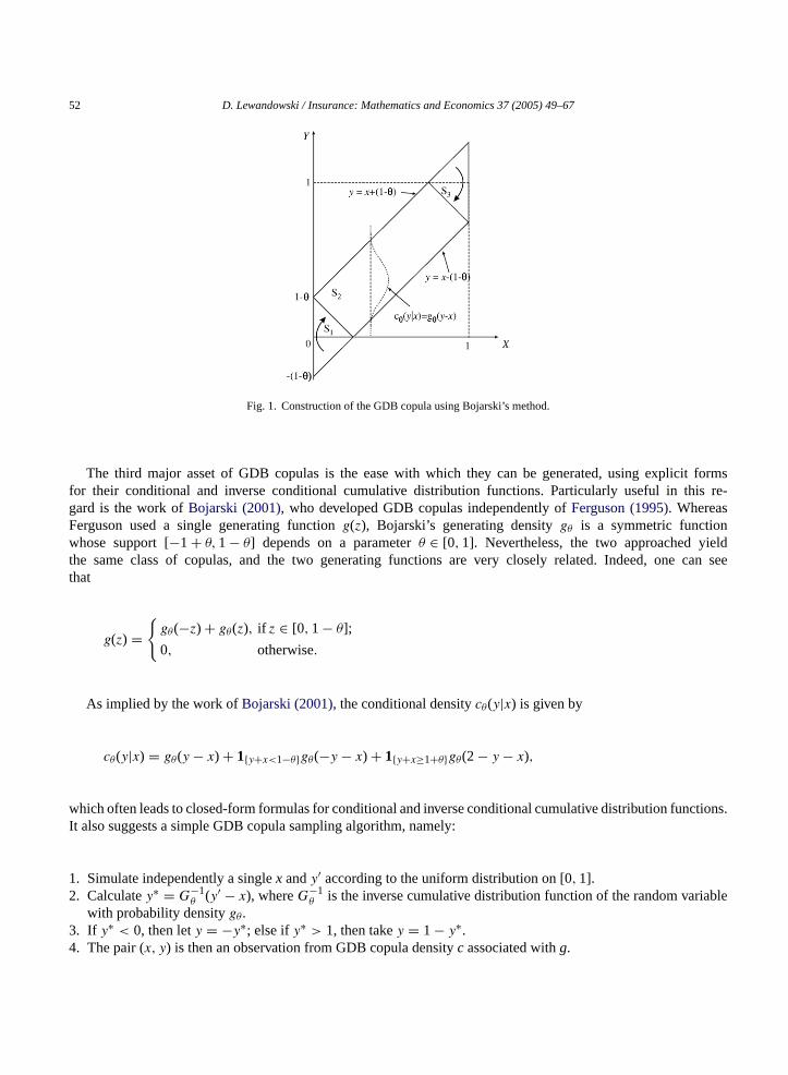
Fig. 1. Construction of the GDB copula using Bojarski’s method.

The third major asset of GDB copulas is the ease with which they can be generated, using explicit formsfor their conditional and inverse conditional cumulative distribution functions. Particularly useful in this re-gard is the work ofBojarski (2001), who developed GDB copulas independently ofFerguson (1995). WhereasFerguson used a single generating functiong(z), Bojarski’s generating densitygθ is a symmetric functionwhose support [−1 + θ, 1 − θ] depends on a parameterθ ∈ [0, 1]. Nevertheless, the two approached yieldthe same class of copulas, and the two generating functions are very closely related. Indeed, one can seethat

g(z) ={

gθ(−z) + gθ(z), if z ∈ [0, 1 − θ];

0, otherwise.

As implied by the work ofBojarski (2001), the conditional densitycθ(y|x) is given by

cθ(y|x) = gθ(y − x) + 1{y+x<1−θ}gθ(−y − x) + 1{y+x≥1+θ}gθ(2 − y − x),

which often leads to closed-form formulas for conditional and inverse conditional cumulative distribution functions.It also suggests a simple GDB copula sampling algorithm, namely:

1. Simulate independently a singlex andy′ according to the uniform distribution on [0, 1].2. Calculatey∗ = G−1

θ (y′ − x), whereG−1θ is the inverse cumulative distribution function of the random variable

with probability densitygθ.3. If y∗ < 0, then lety = −y∗; else ify∗ > 1, then takey = 1 − y∗.4. The pair (x, y) is then an observation from GDB copula densityc associated withg.


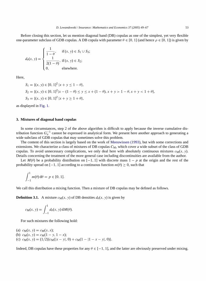
Before closing this section, let us mention diagonal band (DB) copulas as one of the simplest, yet very flexibleone-parameter subclass of GDB copulas. A DB copula with parameterθ ∈ [0, 1] (and henceρ ∈ [0, 1]) is given by

dθ(x, y) =

1

1 − θ, if (x, y) ∈ S1 ∪ S3;

1

2(1− θ), if (x, y) ∈ S2;

0, elsewhere.

Here,

S1 = {(x, y) ∈ [0, 1]2 |x + y ≤ 1 − θ},S2 = {(x, y) ∈ [0, 1]2|x − (1 − θ) ≤ y ≤ x + (1 − θ), x + y > 1 − θ, x + y < 1 + θ},S3 = {(x, y) ∈ [0, 1]2 |x + y ≥ 1 + θ},

as displayed inFig. 1.

3. Mixtures of diagonal band copulas

In some circumstances, step 2 of the above algorithm is difficult to apply because the inverse cumulative dis-tribution functionG−1

θ cannot be expressed in analytical form. We present here another approach to generating awide subclass of GDB copulas that may sometimes solve this problem.

The content of this section is largely based on the work ofMeeuwissen (1993), but with some corrections andextensions. We characterize a class of mixtures of DB copulasCM, which cover a wide subset of the class of GDBcopulas. To avoid unnecessary complications, we only deal here with absolutely continuous mixturescM(x, y).Details concerning the treatment of the more general case including discontinuities are available from the author.

Let M(θ) be a probability distribution on [−1, 1] with discrete mass 1− p at the origin and the rest of theprobability spread on [−1, 1] according to a continuous functionm(θ) ≥ 0, such that

∫ 1

−1m(θ) dθ = p ∈ [0, 1].

We call this distribution a mixing function. Then a mixture of DB copulas may be defined as follows.

Definition 3.1. A mixture cM(x, y) of DB densitiesdθ(x, y) is given by

cM(x, y) =∫ 1

−1dθ(x, y) dM(θ).

For such mixtures the following hold:

(a) cM(x, y) = cM(y, x);(b) cM(x, y) = cM(1 − y, 1 − x);(c) cM(x, y) = (1/2){cM(|x − y|, 0) + cM(1 − |1 − x − y|, 0)}.

Indeed, DB copulas have these properties for anyθ ∈ [−1, 1], and the latter are obviously preserved under mixing.


In view of the above, mixtures of DB densities are in the class of GDB copulas. Our intention in this section isto show that reciprocally, a wide subclass of GDB copulas can be recovered from mixtures of DB copulas.

We begin by observing that since the densitycM(x, y) of a mixture of DB copulas is uniquely determined by itsconditional densitycM(x, 0), the problem of mixing densities of DB copulas can be simplified to mixing conditionaldensities of DB copulas, which are step functions of the form:

dθ(x, 0) =

0, if x ∈ [0, −θ];1

1 + θ, if x ∈ (−θ, 1]

(7)

for θ ≤ 0 and

dθ(x, 0) =

1

1 − θ, if x ∈ [0, 1 − θ];

0, if x ∈ (1 − θ, 1](8)

for θ ≥ 0. These functions are finite for anyθ ∈ (−1, 1). Forθ = 1 or θ = −1, we obtain the so-called Frechet–Hoeffding bounds, andd−1(x, 0) andd1(x, 0) are Dirac delta functions.

We show in Theorem3.2 that for a generating densityg satisfying certain conditions, there exists a mixingfunctionM such that

g(x) =∫ 1

−1dθ(x, 0) dM(θ) =

∫ 1

−1dθ(x, 0)m(θ) dθ + (1 − p)d0(x, 0). (9)

Before stating the result, let us introduce two differentiable functionsg+ andg−, and whose derivatives with respectto x are as follows:

d

dxg+(x) = max

{d

dxg(x), 0

}, g+(0) = 0, (10)

d

dxg−(x) = max

{− d

dxg(x), 0

}, g−(0) = 0. (11)

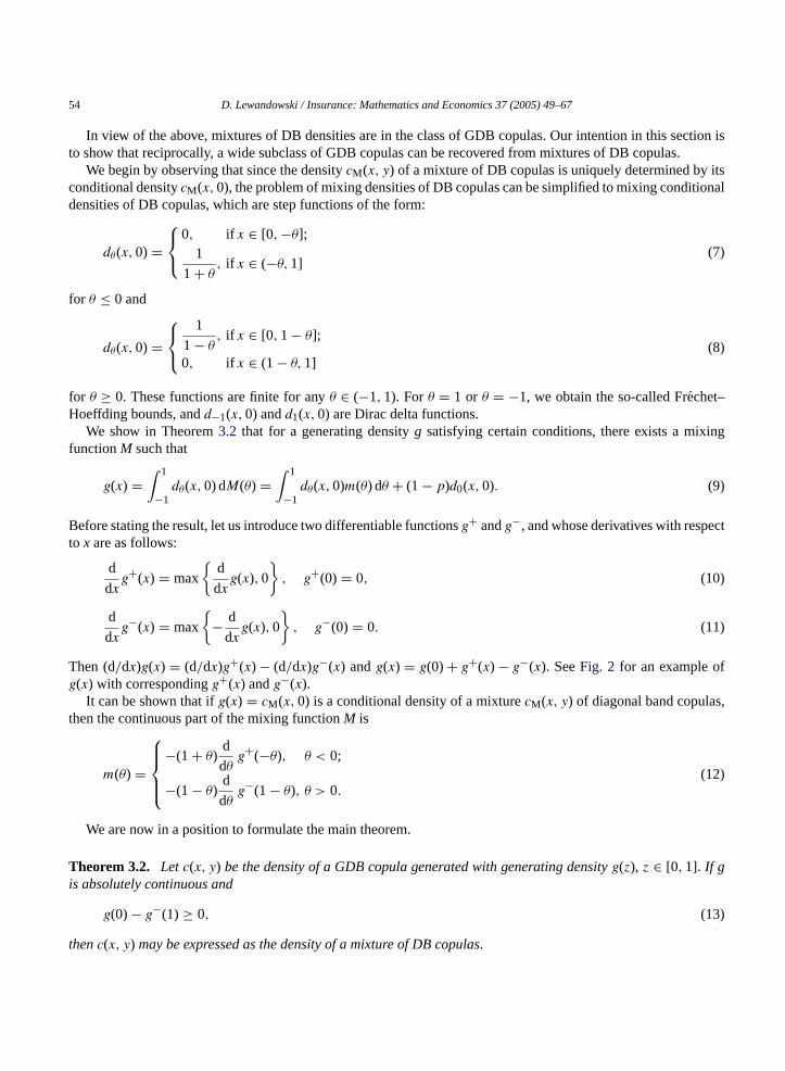
Then (d/dx)g(x) = (d/dx)g+(x) − (d/dx)g−(x) andg(x) = g(0) + g+(x) − g−(x). SeeFig. 2 for an example ofg(x) with correspondingg+(x) andg−(x).

It can be shown that ifg(x) = cM(x, 0) is a conditional density of a mixturecM(x, y) of diagonal band copulas,then the continuous part of the mixing functionM is

m(θ) =

−(1 + θ)d

dθg+(−θ), θ < 0;

−(1 − θ)d

dθg−(1 − θ), θ > 0.

(12)

We are now in a position to formulate the main theorem.

Theorem 3.2. Let c(x, y) be the density of a GDB copula generated with generating densityg(z), z ∈ [0, 1]. If gis absolutely continuous and

g(0) − g−(1) ≥ 0, (13)

thenc(x, y) may be expressed as the density of a mixture of DB copulas.


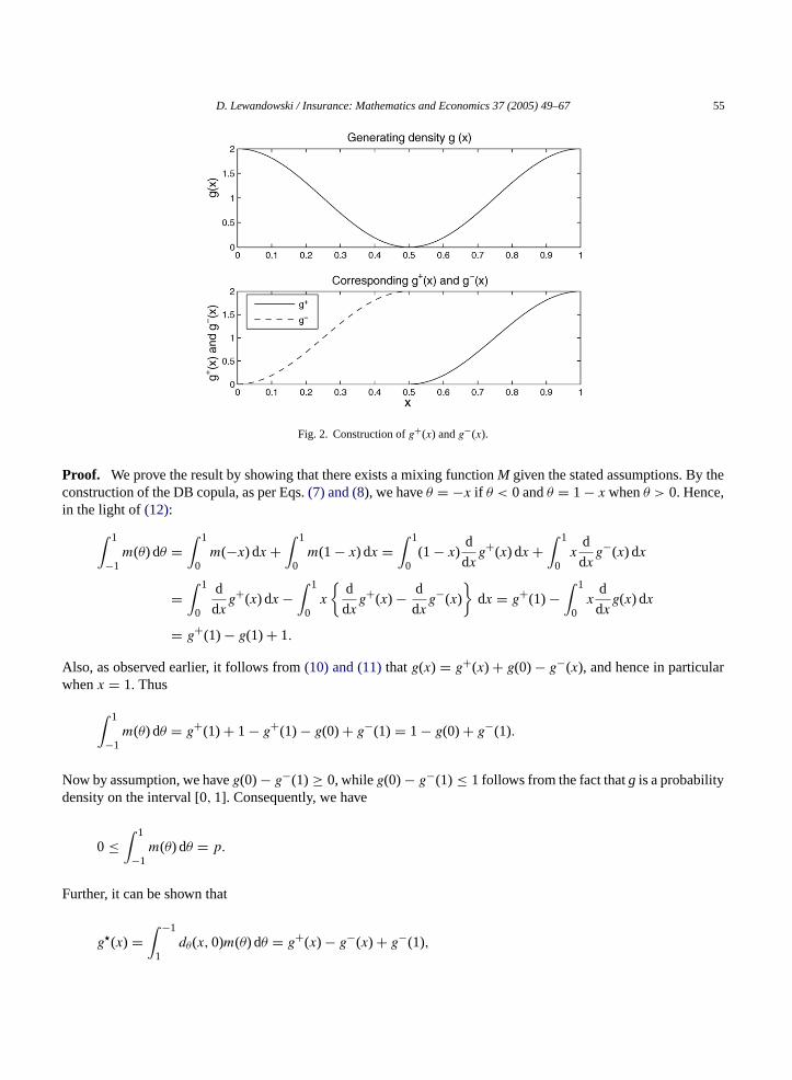
Fig. 2. Construction ofg+(x) andg−(x).

Proof. We prove the result by showing that there exists a mixing functionM given the stated assumptions. By theconstruction of the DB copula, as per Eqs.(7) and (8), we haveθ = −x if θ < 0 andθ = 1 − x whenθ > 0. Hence,in the light of(12):

∫ 1

−1m(θ) dθ =

∫ 1

0m(−x) dx +

∫ 1

0m(1 − x) dx =

∫ 1

0(1 − x)

d

dxg+(x) dx +

∫ 1

0x

d

dxg−(x) dx

=∫ 1

0

d

dxg+(x) dx −

∫ 1

0x

{d

dxg+(x) − d

dxg−(x)

}dx = g+(1) −

∫ 1

0x

d

dxg(x) dx

= g+(1) − g(1) + 1.

Also, as observed earlier, it follows from(10) and (11)thatg(x) = g+(x) + g(0) − g−(x), and hence in particularwhenx = 1. Thus

∫ 1

−1m(θ) dθ = g+(1) + 1 − g+(1) − g(0) + g−(1) = 1 − g(0) + g−(1).

Now by assumption, we haveg(0) − g−(1) ≥ 0, whileg(0) − g−(1) ≤ 1 follows from the fact thatg is a probabilitydensity on the interval [0, 1]. Consequently, we have

0 ≤∫ 1

−1m(θ) dθ = p.

Further, it can be shown that

g�(x) =∫ −1

1dθ(x, 0)m(θ) dθ = g+(x) − g−(x) + g−(1),


which in light of (9) leads tog(x) − g�(x) = g(0) − g−(1) = 1 − p. Therefore

g(x) =∫ −1

1dθ(x, 0)m(θ) dθ + 1 − p =

∫ −1

1dθ(x, 0)m(θ) dθ + (1 − p)d0(x, 0). �

We callg−(1) ≥ 0 the total decrement of functiong. All monotonic density functionsg satisfy condition(13), butalso many non-monotonic functions can be expressed as a mixture of form(9). Note that parameterp can be easilydetermined as

1 −∫ 1

−1m(θ) dθ = 1 − p = min

u∈[0,1]g(u).

Mixtures of DB copulas are very easy to sample from. The procedure is as follows:

1. Simulate a singleθ according toM(θ).2. Simulate a single observation according todθ.3. To generate a pseudo-random sample of sizen, repeat the above stepsn times.

Hence, if it is problematic to deriveG−1θ (z), but easy to obtainM−1(θ) in analytical form, then one can use the

above algorithm, instead of the one that was introduced in Section2. In order for this to work, of course,gθ(z) mustgenerate a GDB copula which is also a mixture of DB copulas.

4. Approximation to the minimally informative GDB copula given the correlation constraint

Part of Meuwissen’s research on mixtures of DB copulas concerned solving a discretized optimization problem.The solution of this problem was a discretized conditional density (step function) that met the conditions of Theorem3.2generalized to the non-continuous case. Therefore, it could be considered a finite mixture of DB densities. Thisdensity generated a GDB copula with minimal mutual information with respect to the uniform distribution under acorrelation constraintρ. Although, GDB copulas had not been formally introduced at that time, Meeuwissen madeuse of the unique property of DB copulas (see Eq.(3)), which was later to be discovered byFerguson (1995),allowing him to introduce the entire class of copulas.

Let us briefly describe the approach Meeuwissen took in order to solve this optimization problem. Assume thatwe are looking for an optimal GDB copulaco(x, y) with minimal relative information with respect to the independentcopula under the correlation constraint generated by a step functionco(x, 0). Fori = 1, . . . , n, let ci(x) denote thevalue of the step function at pointx ∈ (xi−1, xi], wherex0, . . . , xn is a partition ofx ∈ [0, 1] into n intervals ofequal length 1/n (x0 = 0 andxn = 1). Hence, the solution is a vector of lengthn of non-negative real numbers.

Meeuwissen (1993)showed that the relative information of a GDB copulaco(x, y) generated byco(x, 0) withrespect to the uniform background measure is

I(co|u) =n∑

i=1

i−1∑j=1

ci + cj

n2 log

(ci + cj

2

)+

n∑i=1

ci

n2 log(ci), (14)

and the correlationρ realized byco(x, y) is

ρ(X, Y ) = 1 +n∑

i=1

ci{(x4i − x4

i−1) − 2(x3i − x3

i−1)}.


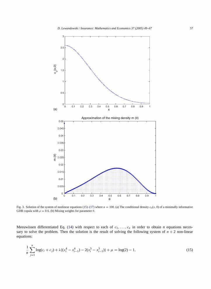
Fig. 3. Solution of the system of nonlinear equations(15)–(17)wheren = 100. (a) The conditional densityco(x, 0) of a minimally informativeGDB copula withρ = 0.6. (b) Mixing weights for parameterθ.

Meeuwissen differentiated Eq.(14) with respect to each ofc1, . . . , cn in order to obtainn equations neces-sary to solve the problem. Then the solution is the result of solving the following system ofn + 2 non-linearequations:

1

n

n∑j=1

log(ci + cj) + λ{(x4i − x4

i−1) − 2(x3i − x3

i−1)} + µ = log(2)− 1, (15)


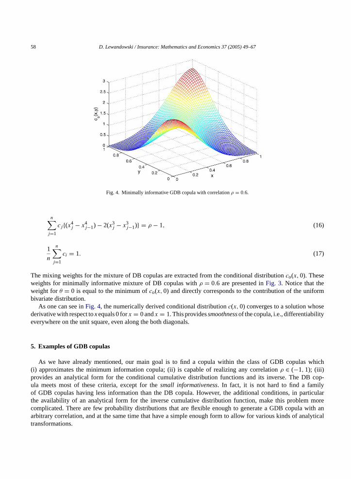
Fig. 4. Minimally informative GDB copula with correlationρ = 0.6.

n∑j=1

cj{(x4j − x4

j−1) − 2(x3j − x3

j−1)} = ρ − 1, (16)

1

n

n∑j=1

ci = 1. (17)

The mixing weights for the mixture of DB copulas are extracted from the conditional distributionco(x, 0). Theseweights for minimally informative mixture of DB copulas withρ = 0.6 are presented inFig. 3. Notice that theweight forθ = 0 is equal to the minimum ofco(x, 0) and directly corresponds to the contribution of the uniformbivariate distribution.

As one can see inFig. 4, the numerically derived conditional distributionc(x, 0) converges to a solution whosederivative with respect toxequals 0 forx = 0 andx = 1. This providessmoothnessof the copula, i.e., differentiabilityeverywhere on the unit square, even along the both diagonals.

5. Examples of GDB copulas

As we have already mentioned, our main goal is to find a copula within the class of GDB copulas which(i) approximates the minimum information copula; (ii) is capable of realizing any correlationρ ∈ (−1, 1); (iii)provides an analytical form for the conditional cumulative distribution functions and its inverse. The DB cop-ula meets most of these criteria, except for thesmall informativeness. In fact, it is not hard to find a familyof GDB copulas having less information than the DB copula. However, the additional conditions, in particularthe availability of an analytical form for the inverse cumulative distribution function, make this problem morecomplicated. There are few probability distributions that are flexible enough to generate a GDB copula with anarbitrary correlation, and at the same time that have a simple enough form to allow for various kinds of analyticaltransformations.


In this section, we introduce three families of GDB copulas which have an analytical form and which, to someextent, comply with the above mentioned desiderata. These copulas can be generated by applying Ferguson’sapproach and achieve non-negative correlations. If negative correlations are desired, one need only make use ofproperty(6).

5.1. Triangular generating function

Assume the following generating function with non-negative parametera:

(a) if 0 ≤ a ≤ 2, ga(z) = −az + 1 + a

2, z ∈ [0, 1],

(b) if a ≥ 2, ga(z) =

−az + √2a, if z ∈

[0,

√2

a

];

0, if z ∈[√

2

a, 1

].

Based on these equations for the generating density of the GDB copula, the conditional and inverse conditionalcumulative distribution functions can be determined and formulated in closed form expressions. However, we shallnot mention them here, in view of their complexity. The relationship between correlationρ and parametera is givenbelow:

a =

5ρ, if ρ ≤ 2

5;

R

([− c

30(ρ − 1)+ 5

c+

√3i

(c

30(ρ − 1)+ 5

c

)]2)

, otherwise;

where

c =(

1350√

2 + 150

√162ρ − 12

ρ − 1

)(ρ − 1)

2

1/3

.

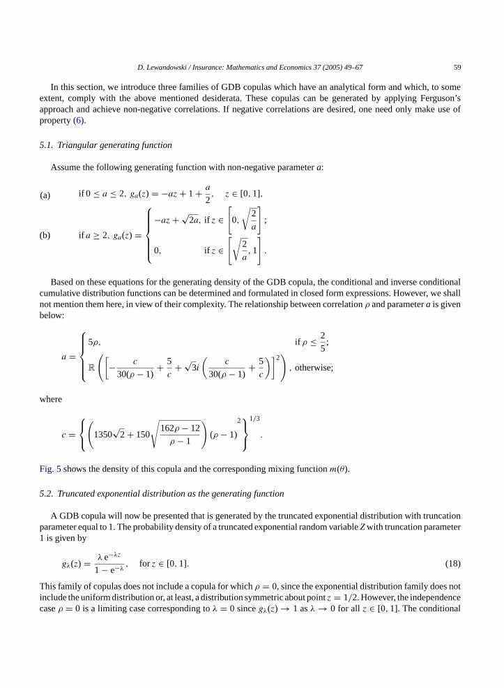
Fig. 5shows the density of this copula and the corresponding mixing functionm(θ).

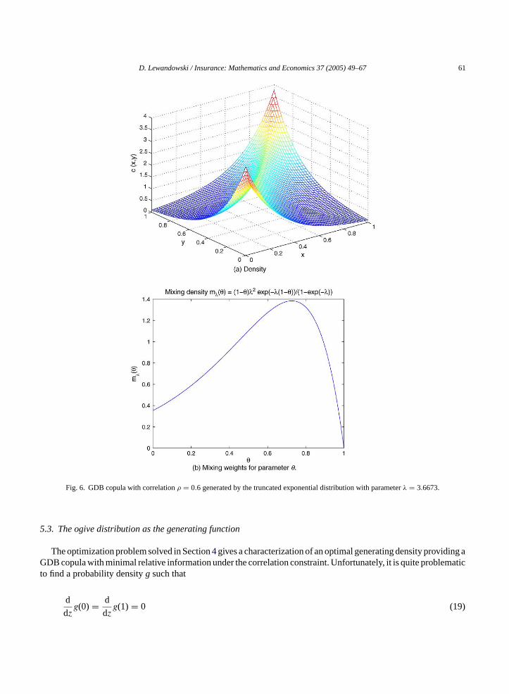
5.2. Truncated exponential distribution as the generating function

A GDB copula will now be presented that is generated by the truncated exponential distribution with truncationparameter equal to 1. The probability density of a truncated exponential random variableZwith truncation parameter1 is given by

gλ(z) = λ e−λz

1 − e−λ, for z ∈ [0, 1]. (18)

This family of copulas does not include a copula for whichρ = 0, since the exponential distribution family does notinclude the uniform distribution or, at least, a distribution symmetric about pointz = 1/2. However, the independencecaseρ = 0 is a limiting case corresponding toλ = 0 sincegλ(z) → 1 asλ → 0 for all z ∈ [0, 1]. The conditional


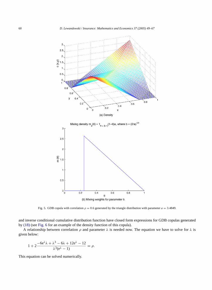
Fig. 5. GDB copula with correlationρ = 0.6 generated by the triangle distribution with parametera = 3.4849.

and inverse conditional cumulative distribution function have closed form expressions for GDB copulas generatedby (18) (seeFig. 6for an example of the density function of this copula).

A relationship between correlationρ and parameterλ is needed now. The equation we have to solve forλ isgiven below:

1 + 2−6eλλ + λ3 − 6λ + 12eλ − 12

λ3(eλ − 1)= ρ.

This equation can be solved numerically.


Fig. 6. GDB copula with correlationρ = 0.6 generated by the truncated exponential distribution with parameterλ = 3.6673.

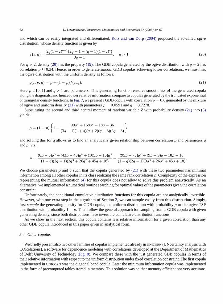
5.3. The ogive distribution as the generating function

The optimization problem solved in Section4gives a characterization of an optimal generating density providing aGDB copula with minimal relative information under the correlation constraint. Unfortunately, it is quite problematicto find a probability densityg such that

d

dzg(0) = d

dzg(1) = 0 (19)


and which can be easily integrated and differentiated.Kotz and van Dorp (2004)proposed the so-calledogivedistribution, whose density function is given by

f (z; q) = 2q(1 − z)q−1{2q − 1 − (q − 1)(1− z)q}3q − 1

, q > 1. (20)

Forq > 2, density(20) has the property(19). The GDB copula generated by the ogive distribution withq = 2 hascorrelationρ ≈ 0.34. Hence, in order to generatesmoothGDB copulas achieving lower correlations, we must mixthe ogive distribution with the uniform density as follows:

g(z; p, q) = p + (1 − p)f (z; q). (21)

Herep ∈ [0, 1] andq > 1 are parameters. This generating function ensures smoothness of the generated copulaalong the diagonals, and hence lower relative information compare to copulas generated by the truncated exponentialor triangular density functions. InFig. 7, we present a GDB copula with correlationρ = 0.6 generated by the mixtureof ogive and uniform density(21)with parametersp = 0.0591 andq = 3.7278.

Substituting the second and third central moment of random variableZ with probability density(21) into (5)yields:

ρ = (1 − p)

{1 − 90q3 + 168q2 + 18q − 36

(3q − 1)(1+ q)(q + 2)(q + 3)(2q + 3)

}

and solving this forq allows us to find an analytically given relationship between correlationρ and parametersqandp, viz.,

p = (6ρ − 6)q5 + (43ρ − 43)q4 + (105ρ − 15)q3

(1 − q)(2q − 1)(3q3 + 26q2 + 45q + 18)+ (95ρ + 73)q2 + (9ρ + 9)q − 18ρ − 18

(1 − q)(2q − 1)(3q3 + 26q2 + 45q + 18).

We choose parametersp andq such that the copula generated by(21) with these two parameters has minimalinformation among all other copulas in its class realizing the same rank correlationρ. Complexity of the expressionrepresenting the mutual information(4) for this copula does not allow to solve this problem analytically. As analternative, we implemented a numerical routine searching for optimal values of the parameters given the correlationconstraint.

Unfortunately, the conditional cumulative distribution functions for this copula are not analytically invertible.However, with one extra step in the algorithm of Section2, we can sample easily from this distribution. Simply,first samplethe generating density for GDB copula, the uniform distribution with probabilityp or the ogive TSPdistribution with probability 1− p. Then follow the general approach for sampling from a GDB copula with givengenerating density, since both distributions have invertible cumulative distribution functions.

As we show in the next section, this copula contains less relative information for a given correlation than anyother GDB copula introduced in this paper given in analytical form.

5.4. Other copulas

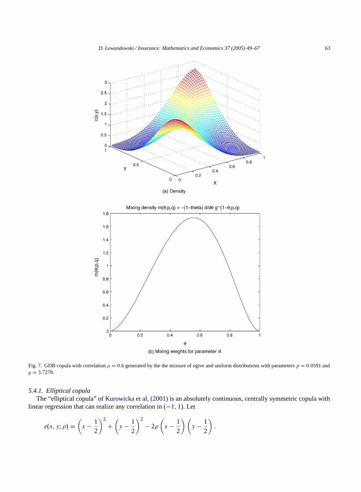
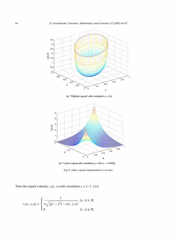
We briefly present also two other families of copulas implemented already inunicorn (UNcertainty analysis wIthCORelations), a software for dependence modeling with correlations developed at the Department of Mathematicsof Delft University of Technology (Fig. 8). We compare these with the just generated GDB copulas in terms oftheir relative information with respect to the uniform distribution under fixed correlation constraint. The first copulaimplemented inunicorn was the diagonal band copula. Later the minimum information copula was implementedin the form of precomputed tables stored in memory. This solution was neither memory efficient nor very accurate.


Fig. 7. GDB copula with correlationρ = 0.6 generated by the the mixture of ogive and uniform distributions with parametersp = 0.0591 andq = 3.7278.

5.4.1. Elliptical copulaThe “elliptical copula” ofKurowicka et al. (2001)is an absolutely continuous, centrally symmetric copula with

linear regression that can realize any correlation in (−1, 1). Let

e(x, y; ρ) =(

x − 1

2

)2

+(

y − 1

2

)2

− 2ρ

(x − 1

2

)(y − 1

2

).


Fig. 8. Other copulas implemented inunicorn.

Then the copula’s densityce(x, y) with correlationρ ∈ (−1, 1) is

ce(x, y; ρ) =

1

π

√14(1 − ρ2) − e(x, y; ρ)

, (x, y) ∈ B;

0, (x, y) �∈ B;


where

B ={

(x, y) ∈ [0, 1]2|e(x, y; ρ) <1

4(1 − ρ)2

}.

This “elliptical copula” is a particular case of the multivariate Pearson type II distribution and should not be confusedwith the notion of meta-elliptical copulas widely used in the literature(Fang et al., 2002; Abdous et al., 2005).

The main disadvantage of this copula is its high mutual information coefficient for given correlation and the factthat it does not include the independent copula.

5.4.2. Frank’s copulaFrank’s copulas is the only class of centrally symmetric Archimedean copulas. It is a one-parameter distribution

with density:

cf (x, y; α) = α(1 − e−α)(e−α(x+y))

{1 − e−α − (1 − e−αx)(1 − e−αy)}2 (22)

for non–zero parameterα. Parameterα > 0 corresponds to positive correlations and vice versa. The independentcopulau(x, y) = 1 can be seen as the limit:

u(x, y) = limα→0

cf (x, y; α).

For additional details about this family of copulas, seeFrank (1979), Nelsen (1986)andGenest (1987).This copula can be problematic to implement in software. The inverse conditional cumulative distribution function

of this copula includes term 1− exp(−α), of which a natural logarithm is computed. Unfortunately, most computerfloating-point number representations would consider this term to be simply equal 0 forα > 37.429. This meansthat in practice, the highest correlation that this copula can realize is of the order of 0.987. A similar term occurs inthe denominator of(22), which also causes numerical problems for large values ofα andx andy close to 1.

For the two copulas presented in this section, conditional and inverse conditional cumulative distribution functionsare given in closed form expressions. However, they differ substantially from each other in the mutual informationthey contain with respect to the independent copula under the correlation constraint.

Table 1The relative information of the minimum information copula for given rank correlation (A) and percent increment for other copulas

Rank correlation,r Copula

A B C D E F G H

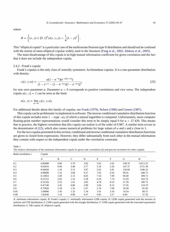
0.1 0.00498 0.80 3.70 3.82 5.02 5.02 538.76 11013.250.2 0.02016 0.94 3.48 3.77 5.16 5.26 247.37 2721.580.3 0.04630 1.10 3.15 3.97 5.62 5.81 150.60 1186.330.4 0.08489 1.35 2.68 4.57 7.03 6.34 99.41 648.720.5 0.13853 1.69 2.15 6.83 7.54 7.09 69.40 399.720.6 0.21212 2.02 1.52 5.28 6.19 7.74 51.03 263.740.7 0.31526 2.35 1.01 3.85 4.78 8.23 37.39 180.750.8 0.47140 2.45 0.86 2.80 3.64 8.12 27.45 124.700.9 0.75820 2.18 1.35 2.07 2.76 7.09 18.58 81.850.95 1.06686 1.45 1.32 1.34 1.91 5.54 14.24 60.510.99 1.82640 1.16 0.98 0.47 0.85 3.27 8.84 37.26

A: minimum information copula; B: Frank’s copula; C: minimally informative GDB copula; D: GDB copula generated with the mixture ofuniform and TSP distribution; E: GDB copula generated with the triangle distribution; F: GDB copula generated with the truncated exponentialdistribution; G: DB copula; H: elliptical copula.


6. Relative information of various copulas

In this section, we compare the mutual information values for the presented copulas as functions of the rankcorrelation. The mutual information values presented inTable 1have been calculated numerically by first generatinga given copula density on a grid of 500× 500 cells, and then approximating the mutual information based on thisdensity. We used this method, because there is no closed form expression for the density of the minimum informationcopula. Therefore, we decided to apply the same numerical method to all copulas considered. The order of thecopulas in the table reflects their performance in terms of the mutual information coefficient, in comparison withthe minimum information copula given the rank correlation. The percentages in columns B–H express the increasein the mutual information coefficient relatively to this value for the minimum information copula.

7. Conclusions

GDB copulas form a very large family of copulas, with the class of mixtures of DB copulas as an importantsubset. Theorem3.2gives a characterization of this subclass. In this paper, we systematized and extended currentknowledge on the class of GDB copulas. The main appeal of the GDB copula is its simple and intuitive construction.Ferguson’s method provides a simple expression for the rank correlation coefficient and straightforward samplingroutine, whereas the Bojarski’s method allows to simplify determining the conditional and inverse conditionalcumulative distribution functions for a given GDB copula.

The copulas presented in this paper can be used to approximate the minimum information copulas. The copulagenerated by the triangle density and the mixture of uniform and ogive TSP distribution can achieve any correlationρ ∈ (−1, 1); the same is true of the copula generated by the truncated exponential density. Having analytical formsfor the conditional cumulative distribution functions and their inverses make these copulas suitable for use in thevine-copula method. Further research on sampling with vines concentrates on overcoming this requirement andhence more freedom in choosing a copula.

Algorithms for generating samples from GDB copulas (satisfying certain conditions) have been proposed. If theinverse cumulativeG−1

θ of the generating densityGθ is given in analytical form, then algorithm 2 can be applied.If this is not the case, but one can sample fromM(θ) then algorithm 3 is available for use.

Acknowledgments

The author would like to express his gratitude to Professor R.M. Cooke, Dr D. Kurowicka from Delft Universityof Technology and Dr J.R. van Dorp from the George Washington University for their comments and helpfulexplanations throughout the research on the topic this paper. Special thanks to the Editor, Professor ChristianGenest, for his enormously deep insights into this paper and editing which helped bringing it to this state. All of uswould like to acknowledge the contribution of Hans Meeuwissen (1966–2004), and express our profound sense ofloss at his recent passing.

References

Abdous, B., Genest, C., Remillard, B., 2005. Statistical Modeling and Analysis for Complex Data Problems, Chapter: Dependence Propertiesof Meta-elliptical Distributions. Kluwer, Dordrecht, The Netherlands, pp. 1–15.

Bedford, T., Cooke, R.M., 2001. Probability density decomposition for conditionally dependent random variables modeled by vines. Annals ofMathematics and Artificial Intelligence 32, 245–268.

Bedford, T.J., Cooke, R.M., 2002. Vines—a new graphical model for dependent random variables. The Annals of Statistics 30, 1031–1068.


Bojarski, J., 2001. A New Class of Band Copulas—Distributions with Uniform Marginals, Technical Publication. Institute of Mathematics,Technical University of Zielona Gora.

Cooke, R.M., 1991. Experts in Uncertainty. Oxford University Press.Cooke, R.M., 1997. Markov and entropy properties of tree- and vine-dependent variables. Proceedings of the ASA Section on Bayesian Statistical

Science.Cooke, R.N., Waij, R., 1986. Monte Carlo sampling for generalized knowledge dependence, with application to human reliability. Risk Analysis

6, 335–343.Fang, H.-B., Fang, K.-T., Kotz, S., 2002. The meta-elliptical distributions with given marginals. Journal of Multivariate Analysis 82, 1–16.Ferguson, T.S., 1995. A class of bivariate uniform distributions. Statistical Papers 36, 31–40.Frank, M.J., 1979. On the simultaneous associativity off (x, y) andx − y − f (x, y). Aequationes Mathematicae 19, 194–226.Genest, C., 1987. Frank’s family of bivariate distributions. Biometrika 74, 549–555.Kotz, S., van Dorp, J.R., 2004. Beyond Beta, Other Continuous Families of Distributions with Bounded Support and Applications. World

Scientific Press, Singapore.Kurowicka, D., Cooke, R.M., 2003. A parametrization of positive definite matrices in terms of partial correlation vines. Linear Algebra and its

Applications 372, 225–251.Kurowicka, D., Misiewicz, J., Cooke, R.M., 2001. Elliptical copulae. Monte Carlo Simulation, Schueller and Spanos. Balkema, Rotterdam, pp.

209–214.Meeuwissen, A.M.H., 1993. Dependent random variables in uncertainty analysis. PhD Thesis. Delft University of Technology, Delft, The

Netherlands.Meeuwissen, A.M.H., Bedford, T., 1997. Minimally informative distributions with given rank correlation for use in uncertainty analysis. Journal

of Statistical Computation and Simulation 57, 143–174.Nelsen, R.B., 1986. Properties of a one-parameter family of bivariate distributions with specified marginals. Communications in Statistics,

Theory and Methods 15, 3277–3285.

generalized diagonal band copulas

Documents