generalizations of orthogonal polynomials · qkpll(z l k) = z t 1 k=0 qkt k! 1 l=0 plt l! d (t) = z...
TRANSCRIPT

Generalizations of orthogonalpolynomials
A. Bultheel, Annie Cuyt, W. Van Assche,
M. Van Barel, B. Verdonk
Report TW375, December 2003
Katholieke Universiteit LeuvenDepartment of Computer ScienceCelestijnenlaan 200A – B-3001 Heverlee (Belgium)

Generalizations of orthogonalpolynomials
A. Bultheel, Annie Cuyt, W. Van Assche,
M. Van Barel, B. Verdonk
Report TW375, December 2003
Department of Computer Science, K.U.Leuven
We give a survey of recent generalizations for orthogonal polynomials thatwere recently obtained. It concerns not only multidimensional (matrix andvector orthogonal polynomials) and multivariate versions, or multipole (or-thogonal rational functions) variants of the classical polynomials but alsoextensions of the orthogonality conditions (multiple orthogonality). Mostof these generalizations are inspired by the applications in which they areapplied. We also give a glimpse of the applications, but they are usuallyalso generalizations of applications where classical orthogonal polynomialsplay a fundamental role: moment problems, numerical quadrature, rationalapproximation, linear algebra, recurrence relations, random matrices.
Abstract
Keywords : system identification, orthogonal rational functions, least squares.AMS(MOS) Classification : Primary : 93B30, Secondary : 42C05, 93E24

WOG project J. Comput. Appl. Math., Preprint 1 December 2003 1
Generalizations of orthogonal polynomials ?
A. Bultheel 1
Dept. Computer Science (NALAG), K.U.Leuven,Celestijnenlaan 200 A, B-3001 Leuven, Belgium.
A. Cuyt
Dept. Mathematics and Computer Science, Universiteit Antwerpen,Middelheimlaan 1, B-2020 Antwerpen, Belgium.
W. Van Assche 2
Dept. Mathematics, K.U.LeuvenCelestijnenlaan 200B, B-3001 Leuven, Belgium.
M. Van Barel 1
Dept. Computer Science (NALAG), K.U.Leuven,Celestijnenlaan 200 A, B-3001 Leuven, Belgium.
B. Verdonk
Dept. Mathematics and Computer Science, Universiteit Antwerpen,Middelheimlaan 1, B-2020 Antwerpen, Belgium.
Abstract
We give a survey of recent generalizations for orthogonal polynomials that were recently obtained.It concerns not only multidimensional (matrix and vector orthogonal polynomials) and multivariateversions, or multipole (orthogonal rational functions) variants of the classical polynomials but alsoextensions of the orthogonality conditions (multiple orthogonality). Most of these generalizations areinspired by the applications in which they are applied. We also give a glimpse of the applications,but they are usually also generalizations of applications where classical orthogonal polynomials playa fundamental role: moment problems, numerical quadrature, rational approximation, linear algebra,recurrence relations, random matrices.
Key words: Orthogonal polynomials, rational approximation, linear algebra2000 MSC: 42C10, 33D45, 41A, 30E05, 65D30, 46E35
This paper is dedicated to Olav Njastad on the occasion of his 70th birthday.
1
1 Introduction
Since the fundamental work of Szego [46], orthogonal polynomials have been a basic tool inthe analysis of basic problems in mathematics and engineering. For example moment problems,numerical quadrature, rational and polynomial approximation and interpolation, and all thedirect or indirect applications of these techniques in engineering and applied problems, theyare all indebted to the basic properties of orthogonal polynomials.
The first thing one needs is an inner product defined on the space of polynomials. There areseveral formalizations of this concept. For example, one can define a positive definite Hermitianlinear functional M [·] on the space of polynomials. This means the following. Let Πn the spaceof polynomials of degree at most n and Π the space of all polynomials. The dual space ofΠn is Πn∗, namely the space of all linear functionals. With respect to a set of basis functions{B0, B1, . . . , Bn} that span Πn for n = 0, 1, . . ., it is clear that a polynomial has a uniquelydefined set of coefficients, representing this polynomial. Thus, given a nested basis of Π, we canidentify the complex polynomials Πn with the space C
(n+1)×1 of complex (n + 1) × 1 columnvectors.
Suppose the dual space is spanned by a sequence of basic linear functionals {Lk}∞k=0, anddefine Πn∗ = span{L0, L1, . . . , Ln} for n = 0, 1, 2, . . .. Then the dual subspace Πn∗ can beidentified with C
1×(n+1), the space of complex 1 × (n + 1) row vectors. Now, given a sequenceof linear functionals {Lk}∞k=0, we say that a sequence of polynomials {Pk}∞k=0 with Pk ∈ Πk, isorthonormal with respect to the sequence of linear functionals {Lk}∞k=0 with Lk ∈ Πk∗, if
Lk(Pl) = δkl, k, l = 0, 1, 2 . . . .
Hereby we have to assure some non-degeneracy, which means that the moment matrix of thesystem is Hermitian positive definite. This moment matrix is defined as follows. Consider thebasis B0, B1, . . . in Π and a basis L0, L1, . . . for the dual space Π∗, then the moment matrix is
? This work is partially supported by the Fund for Scientific Research (FWO) via the ScientificResearch Network “Advanced Numerical Methods for Mathematical Modeling”, grant #WO.012.01N.1 The work of these authors is partially supported by the Fund for Scientific Research (FWO)via the projects G.0078.01 “SMA: Structured Matrices and their Applications”, G.0176.02 “AN-CILA: Asymptotic aNalysis of the Convergence behavior of Iterative methods in numerical LinearAlgebra”, G.0184.02 “CORFU: Constructive study of Orthogonal Functions”, G.0455.04 “RHPH:Riemann-Hilbert problems, random matrices and Pade-Hermite approximation”, the Research Coun-cil K.U.Leuven, project OT/00/16 “SLAP: Structured Linear Algebra Package”, and the BelgianProgramme on Interuniversity Poles of Attraction, initiated by the Belgian State, Prime Minister’sOffice for Science, Technology and Culture. The scientific responsibility rests with the authors.2 The work of this author is partially supported by the Fund for Scientific Research (FWO) via theprojects G.0184.02 “CORFU: Constructive study of Orthogonal Functions” and G.0455.04 “RHPH:Riemann-Hilbert problems, random matrices and Pade-Hermite approximation”.
2

the infinite matrix
M =
m00 m01 m02 . . .
m10 m11 m12 . . .
m20 m21 m22 . . ....
......
. . .
, with mij = Li(Bj).
It is Hermitian positive definite if Mkk = [mij]ki,j=0 is Hermitian positive definite for all k =
0, 1, . . ..
In some formal generalizations, positive definiteness may not be necessary; a nondegeneracycondition is then sufficient. In other applications it is even not really necessary to impose thisnondegeneracy condition, and in that case there should be some notion of block orthogonalitybecause the existence of an orthonormal set is not guaranteed anymore.
Note that if the coefficients of P ∈ Πn and Q∗ ∈ Πn∗ are given by p = [p0, p1, . . .]T and
q = [q0, q1, . . .] respectively, then Q∗(P ) = qMp.
Classical cases fall into this framework. For example consider a positive measure µ of a finiteor infinite interval I on the real line, a basis 1, x, x2, . . . for the space of real polynomials and abasis of linear functionals L0, L1, . . . defined by
Lk(P ) =∫
I
xkP (x)dµ(x),
then we can choose Lk as the dual of the polynomial xk and therefore introduce an inner productin Π as
〈Q,P 〉 =∞∑
k=0
∞∑
l=0
qkpl
⟨xk, xl
⟩=
∞∑
k=0
∞∑
l=0
qkplLk(xl) = Q∗(P ),
if Q∗ =∑∞
k=0 qkLk, Q(x) =∑∞
k=0 qkxk, and P (x) =
∑∞k=0 pkx
k. If µ is a positive measure, themoment matrix is guaranteed to be positive definite.
Note that in this case we need to define only one linear functional L on Π to determine thewhole moment matrix. It is defined as L(xi) =
∫Ixidµ(x). The moment matrix is completely
defined by the sequence mk = L(xk), k = 0, 1, 2, . . ..
Another famous case is obtained by orthogonality on the unit circle. Consider T = {t ∈ C :|t| = 1} and a positive measure on T. The set of complex polynomials are spanned by 1, z, z2, . . .and we consider linear functionals Lk defined by
Lk(zl) = L(zl−k) =
∫
T
tl−kdµ(t), k, l = 0, 1, 2, . . . .
3

Thus we can again use only one linear functional L(P (z)) =∫TP (t)dµ(t) and define a positive
definite Hermitian inner product on the set of complex polynomials by
〈Q,P 〉=
⟨ ∞∑
k=0
qkzk,
∞∑
l=0
plzl
⟩=
∞∑
k=0
∞∑
l=0
qkpl
⟨zk, zl
⟩
=∞∑
k=0
∞∑
l=0
qkplLk(zl) =
∞∑
k=0
qkLk
( ∞∑
l=0
plzl
)= Q∗(P )
=∞∑
k=0
∞∑
l=0
qkplL(zl−k) =∫
T
( ∞∑
k=0
qkt−k
)( ∞∑
l=0
pltl
)dµ(t)
=∫
T
Q∗(t)P (t)dµ(t).
where we have abused the notation Q∗ for both the linear functional Q∗ =∑∞
k=0 qkLk and forthe dual polynomial Q∗(z) =
∑∞k=0 qkz
−k, which is the dual of Q(z) =∑∞
k=0 qkzk, and we have
set P (z) =∑∞
l=0 plzl. Note that here the linear functional L is defined on the space of Laurent
polynomials Λ = span{zk : k ∈ Z}. The moment matrix is completely defined by the onedimensional sequence mk = L(zk), k ∈ Z, and because µ is positive, it is sufficient to give mk,k = 0, 1, 2 . . . because m−k = L(z−k) = L(zk) = mk.
Note that in the case of polynomials orthogonal on an interval on the real line, the momentmatrix [mkl] is real and has a Hankel structure and in the case of orthogonality on the circle,then the moment matrix is complex Hermitian and has a Toeplitz structure. This explains ofcourse why a single sequence defines the whole matrix in both cases.
One of the basic problems that is considered, is the moment problem where it is required torecover from a positive definite moment matrix a representation of the inner product. In theexamples above, it is to find the positive measure µ from the (positive) moment sequence {mk}.
The relation with structured linear algebra problems has given rise to an intensive research onfast algorithms for the solution of linear systems of equations and other linear algebra problems.The duality between real Hankel and complex Toeplitz is in this context a natural distinction.However, what is possible for one case is usually also true in some form for the other case.
For example, the Hankel structure is at the heart of the famous three-term recurrence relationfor orthogonal polynomials. For 3 successive orthogonal polynomials φn, φn−1, φn−2 there areconstants An, Bn, and Cn with An > 0 and Cn > 0 such that
φn(x) = (Anx+Bn)φn−1(x) − Cnφn−2(x), n = 2, 3, . . .
Closely related to this recurrence is the Christoffel-Darboux relation which gives a closed formexpression for the (reproducing) kernel kn(z, w)
kn(x, y) :=n∑
k=0
φn(x)φn(y) =κn
κn+1
φn+1(x)φn(y) − φn(x)φn+1(y)
x− y
4

where κn is the highest degree coefficient of φn. All three items: orthogonality, three-termrecurrence, and a Christoffel-Darboux relation are in a sense equivalent. The Favard theoremstates that if there is a three-term recurrence relation with certain properties, then the sequenceof polynomials that it generates will be a sequence of orthogonal polynomials with respect tosome inner product. Brezinski showed [12] that the Christoffel-Darboux relation is equivalentwith the recurrence relation.
In the case of the unit circle, another fundamental type of recurrence relation is due to Szego.The recursion is of the form
φk+1(z) = ck+1[zφk(z) + ρk+1φ∗k(z)]
where for any polynomial Pk of degree k we set
P ∗k (z) = zkPk∗(z) = zkPk(1/z),
so that φ∗k is the reciprocal of φk, ρk+1 is a Szego parameter and ck+1 = (1 − |ρk+1|2)−1/2 is a
normalizing constant. This recurrence relation plays the same fundamental role as the three-term recurrence relation does for orthogonality on (part of) the real line. There is a relatedFavard-type theorem and a Christoffel-Darboux-type of relation that now has the complex form
kn(z, w) :=n∑
k=0
φn(z)φn(w) =φ∗
n+1(z)φ∗n+1(w) − φn+1(z)φn+1(w)
1 − zw.
Another basic aspect of orthogonal polynomials is rational approximation. Rational approxima-tion is given through the fact that truncating a continued fraction gives an approximant for thefunction to which it converges. The link with orthogonal polynomials is that continued fractionsare essentially equivalent with three-term recurrence relations, and orthogonal polynomials onan interval are known to satisfy such a recurrence. In fact if the orthogonal polynomials aresolutions of the recurrence with starting values φ−1 = 0 and φ0 = 1, then an independent solu-tion can be obtained as a polynomial sequence {ψk} by using the initial conditions ψ−1 = −1and ψ0 = 0. It turns out that
ψn(x) = L
(φn(x) − φn(y)
x− y
)=∫
I
φn(x) − φn(y)
x− ydµ(x)
where L is the linear functional defining the inner product on I ⊂ R. (Note that ψn is apolynomial of degree n− 1.) Therefore, the nth approximant of the continued fraction
1
A1x+B1
− C2
A2z +B2
− C3
A3z +B3
− · · ·
is given by ψn(x)/φn(x). The continued fraction converges to the Stieltjes transform or Cauchy
5

transform (note the Cauchy kernel C(x, y) = 1/(x− y))
Fµ(x) = L
(1
x− y
)=∫
I
dµ(y)
x− y.
The approximant is a Pade approximant at ∞ because
ψn(x)
φn(x)=m0
x+m1
x2+ · · · + m2n−1
x2n+ O
(1
x2n+1
)= Fµ(x) + O
(1
x2n+1
), x→ ∞.
All the 2n + 1 free parameters in the rational function ψn/φn of degree n are used to fit thefirst 2n+ 1 coefficients in the asymptotic expansion of Fµ at ∞.
Again, there is an analog situation for the unit circle case. Then the function that is approx-imated is a Riesz-Herglotz transform
Fµ(z) =∫
T
t+ z
t− zdµ(t).
where now the Riesz-Herglotz kernel D(t, z) = (t+ z)/(t− z) is used. This function is analyticin the open unit disk and has a positive real part for |z| < 1. It is therefore a Caratheodoryfunction. By the Cayley transform, one can map the right half plane to the unit disk, bywhich we can transform a Caratheodory function F into a Schur function, since indeed S(z) =(Fµ(z) − Fµ(0))/[z(Fµ(z) + Fµ(0))] is a function analytic in the unit disk and |S(z)| < 1 for|z| < 1. It is in this framework that Schur has developed his famous algorithm to check whethera function is in the Schur class. It is based on the simple lemma saying that S is in the Schurclass if and only if |S(0)| < 1 and S1(z) = 1
z(S(z)− S(0))/(1− S(0)S(z)) is in the Schur class.
Applying this lemma recursively gives the complete test. This kind of test is closely related to astability test for polynomials in discrete time linear system theory or the solution of differenceequations. It is known as the Jury test. A similar derivation exists for the case of an intervalon the real line, which leads to the Routh-Hurwitz test, which is a bit more involved.
Note also that the moments show up as Fourier-Stieltjes coefficients of Fµ because
Fµ(z) =∫
T
[1 + 2
∞∑
k=1
zk
tk
]dµ(t) = m0 + 2
∞∑
k=1
m−kzk.
It is again possible to construct a continued fraction whose approximants are alternatinglyψn/φn and ψn∗/φn∗, and these are two-point Pade approximants at the origin and infinity forFµ in a linearized sense.
I.e., one has
Fµ(z) + ψn(z)/φn(z) =O(z−n−1), z → ∞,
Fµ(z)φn(z) + ψn(z) =O(zn), z → 0,
6

and
Fµ(z)φn∗(z) − ψn∗(z) =O(z−n), z → ∞,
Fµ(z) − ψn∗(z)/φn∗(z) =O(zn+1), z → 0.
Here the ψn are defined by
ψn(z) = L (D(t, z)[ψn(t) − φn(z)]) =∫
T
t+ z
t− z[φn(t) − φn(z)]dµ(t).
The term two-point Pade approximant is justified by the fact that the interpolation is in thepoints 0 and ∞ and the number of interpolation conditions equals the degrees of freedom in therational function of degree n. Since φn∗/ψn∗ is a rational Caratheodory function, it is a solutionof a partial Caratheodory coefficient problem. This is the problem of finding a Caratheodoryfunction with given coefficients for its expansion at the origin. To a large extent the Schurinterpolation problem, the Caratheodory coefficient problem and the trigonometric momentproblem are all equivalent.
Another important aspect directly related to orthogonal polynomials and the previous approx-imation properties is numerical quadrature formulas. By a quadrature formula for the integralIµ(f) :=
∫If(x)dµ(x) is meant a formula of the form In(f) :=
∑nk=1wnkf(ξnk). The knots
ξnk should be in distinct points that are preferably in I, the support of the measure µ, andthe weights are preferably positive. Both these requirements are met by the Gauss quadratureformulas, i.e., when the ξnk are chosen as the n zeros of the orthogonal polynomial φn. Theweights or Christoffel numbers are then given by wnk = 1/kn(ξnk, ξnk) = 1/
∑nk=0[φn(ξnk)]
2 andthe quadrature formula has the maximal domain of validity in the set of polynomials. Thismeans that In(f) = Iµ(f) for all f that are polynomials of degree at most 2n − 1. It can beshown that there is no n-point quadrature formula that will be exact for all polynomials ofdegree 2n, so that the polynomial degree of exactness is maximal.
In the case of the unit circle, the integral Iµ(f) :=∫Tf(t)dµ(t) is again approximated by
a formula of the form In(f) :=∑n
k=1wnkf(ξnk), where now the knots are preferably on theunit circle. However, the zeros of φn are known to be strictly less than one in absolute value.Therefore, the para-orthogonal polynomials are introduced as
Qn(z, τ) = φn(z) + τφ∗n(z), τ ∈ T.
It is known that these polynomials have exactly n simple zeros on T and thus they can be usedas knots for a quadrature formula. If the corresponding weights are chosen as before, namelywnk = 1/kn(ξnk, ξnk) = 1/
∑nk=0 |φn(ξnk)|2, then these are obviously positive and the quadrature
formula becomes a Szego formula, again with maximal domain of validity, namely In(f) = Iµ(f)for all f that are in the span of {z−n+1, . . . , zn−1}, a subspace of dimension 2n− 1 in the spaceof Laurent polynomials.
We have just given the most elementary account of what orthogonal polynomials are relatedto. Many other aspects are not even mentioned: for example the tridiagonal Jacobian operator
7
(real case) or the unitary Hessenberg operator (circle case) which catch the recurrence relationin one operator equation, also the deep studies by Geronimus, Freud and many others to studythe asymptotics of orthogonal polynomials, their zero distribution, and many other propertiesunder various assumptions on the weights and/or on the recurrence parameters [25,28,36,37,45],there are the differential equations like Rodrigues formulas and generating functions that holdfor so called classical orthogonal polynomials, the whole Askey-Wilson scheme, introducing awealth of extensions for the two simplest possible schemes that were introduced above.
Also from the application side there are many generalizations, some are formal [16] orthogon-ality relations inspired by fast algorithms for linear algebra, some are matrix and vector formsof orthogonal polynomials which are often inspired by linear system theory and all kind ofgeneralizations of rational interpolation problems. And so further and so on.
In this paper we want to give a survey of recent achievements about generalizations of orthogonalpolynomials. What we shall present is just a sample of what is possible and reflects the interestof the authors. It is far from being a complete survey. Nevertheless, it is an illustration of thediversity of possibilities that are still open for further research.
2 Orthogonal rational functions
One of the recent generalizations of orthogonal polynomials that has emerged during the lastdecade is the analysis of orthogonal rational functions. They were first introduced by Djrbashianin the 1960’s. Most of his papers appeared in the Russian literature. An accessible survey inEnglish can be found in [22]. Details about this section can be found in the book [14]. For asurvey about their use in numerical quadrature see the survey paper [15], for another surveyand further generalizations see [13]. Several results about matrix-valued orthogonal rationalfunctions are found in [34,26,27].
2.1 Orthogonal rational functions on the unit circle
Some connections between orthogonal polynomials and other related problems were given inthe introduction to this paper. The simplest way to introduce the orthogonal rational functionsis to look at a slight generalization of the Schur lemma. With the Schur function constructedfrom a positive measure µ as it was in the introduction, the lemma says that if µ has infinitelymany points of increase, then for some α ∈ D = {z ∈ C : |z| < 1} we have S(α) ∈ D and S1
is again a Schur function if S1(z) = Sα(z)/ζα(z) with Sα(z) = (S(z) − S(α))/(1 − S(α)S(z))and ζα(z) = (z−α)/(1−αz). As in the polynomial case, a recursive application of this lemmaleads to some continued fraction-like algorithm that computes for a given sequence of points{αk}∞k=1 ⊂ D (with or without repetitions) a sequence of parameters ρk = Sk(αk+1) that are allin D and that are generalizations of the Szego parameters.
Thus instead of taking all the αk = 0, which yields the Szego polynomials, we obtain a mul-tipoint generalization. The multipoint generalization of the Schur algorithm is the algorithmof Nevanlinna-Pick. It is well known that this algorithm constructs rational approximants of
8
increasing degree that interpolate the original Schur function S in the successive points αk.Suppose we define the successive Schur functions Sn(z) as the ratio of two functions analyticin D, namely Sn(z) = ∆n1(z)/∆n2(z), then the Schur recursion reads (ρn+1 = Sn(αn+1) andζn(z) = zn
z−αn
1−αnzwith zn = 1 if αn = 0 and zn = αn/|αn| otherwise)
[∆n+1,1 ∆n+1,2] = [∆n,1 ∆n,2]
1 −ρn+1
−ρn+1 1
1/ζn+1 0
0 1
.
This describes the recurrence for the tails. The inverse recurrence is the recurrence for thepartial numerators and denominators of the underlying continued fraction:
[φn+1 φ∗n+1] = [φn φ∗
n]
ζn+1 0
0 1
1√1 − |ρn+1|2
1 ρn+1
ρn+1 1
.
When starting with φ0 = φ∗0 = 1, this generates rational functions φn which are of degree n
and which are in certain spaces with poles among the points {1/αk}
φn, φ∗n ∈ Ln = span{B0, B1, . . . , Bn} =
{pn
πn
: pn ∈ Πn
}
where πn(z) =∏n
k=1(1 − αjz) and the finite Blaschke products are defined by
B0 = 1, Bk = ζ1ζ2 · · · ζk.
Moreover, it is easily verified that φn(z) = Bn(z)φn∗(z) where φn∗(z) = φn(1/z). This shouldmake clear that the recurrence
φn+1(z) = cn+1[ζn+1(z)φn(z) + ρn+1φ∗n(z)], cn+1 = (1 − |ρn+1|2)−1/2
is a generalization of the Szego recurrence relation.
Transforming back from the Schur to the Caratheodory domain, the approximants of the Schurfunction correspond to rational approximants of increasing degree that interpolate the functionsFµ in the points αk. Defining the rational functions of the second kind ψn exactly as in thepolynomial case, then we have multipoint Pade approximants since
zBn(z)[Fµ(z) + ψn(z)/φn(z)] is holomorfic in 1 < |z| ≤ ∞[zBn−1(z)]
−1[Fµ(z)φn(z) + ψn(z)] is holomorfic in 0 ≤ |z| < 1
and
[zBn−1(z)][Fµ(z)φn∗(z) − ψn∗(z)] is holomorfic in 1 < |z| ≤ ∞[zBn(z)]−1[Fµ(z) − ψn∗(z)/φn∗(z)] is holomorfic in 0 ≤ |z| < 1.
9

The φk correspond to orthogonal rational functions with respect to the Riesz-Herglotz measureof Fµ. They can be obtained by a Gram-Schmidt orthogonalization procedure applied to thesequence B0, B1, . . .. If all αk are zero, the poles are all at infinity and the Szego polynomialsemerge as a special case.
Just as Fµ is a moment generating function by applying the linear functional L to the (formal)expansion of the Riesz-Herglotz kernel, we now have
Fµ(z) =∫
T
[1 + 2z
∞∑
k=1
π∗n−1(z)
π∗n(t)
]dµ(t) = m0 + 2
∞∑
k=1
m−kzπ∗n−1(z)
where the generalized moments are now defined by
m−k =∫
T
dµ(t)
π∗k(t)
, π∗k(z) =
k∏
j=1
(z − αj).
Note that also in this generalized rational case, we can define a linear functional L operating onL = ∪∞
k=0Lk via the definition of the moments L(1) = m0 and L(1/π∗k) = m−k for k = 1, 2, . . .. If
L is a real functional, then by taking the complex conjugate of the latter and by partial fractiondecomposition, it should be clear that the functional is actually defined on the space L·L∗ whereL∗ = {f : f∗ ∈ L}. Thus, we can use L to define a complex Hermitian inner product on L and sothe use of the orthogonal rational functions is possible for the solution of the generalized momentproblem. The essence of the technique is to note that the quadrature formula whose knots arethe zeros {ξnk}n
k=1 of the para-orthogonal function Qn(z, τ) = φn(z)+τφ∗n(z) (they are all simple
and lie on T) and as weights the numbers 1/kn−1(ξnk, ξnk) > 0, then this quadrature formula isexact for all rational functions in Ln−1 · Ln−1. It then follows that under certain conditions thediscrete measure that corresponds to the quadrature formula converges for n → ∞ in a weaksense to a solution of the moment problem. The conditions for this to hold are now involved,not only with the moments, but also with the selection of the sequence of points {αk}∞k=q ⊂ D.A typical condition being that
∑∞k=1(1−|αk|) = ∞, i.e., the condition that makes the Blaschke
product∏∞
k=1 ζk diverge to zero.
2.2 Orthogonal rational functions on the real line
About the same discussion can be given for orthogonal rational functions on the real axis. Ifhowever we want the polynomials (which are rational functions with poles at ∞) to come outas a special case, then the natural multipoint generalization is to consider a sequence of pointsthat are all on the (extended) real axis R = R∪{∞}. For technical reasons, we have to excludeone point. Without loss of generality, we shall assume this to be the point at infinity. Thus weconsider the sequence of points {αk}∞k=1 ⊂ R and we define πn(z) =
∏nk=1(1−αkz). The spaces
of rational functions we shall consider are given by Ln = {pn/πn : pn ∈ Πn}. If we define thebasis functions b0 = 1, bn(z) = zn/πn(z), k = 1, 2, . . ., then orthogonalization of this basis givesthe orthogonal rational functions φn. The inner product can be defined in terms of a positive
10
measure on R via (we assume functions with real coefficients)
〈f, g〉 =∫
R
f(x)g(x)dµ(x), f, g ∈ L,
or via some positive linear functional L defined on the space L · L. Such a linear functional isdefined if we know the moments
mkl = L(bkbl), k, l = 0, 1, . . .
Thus in this case, defining the functional on L or on L·L are two different things. In the first casewe only need the moments mk0, in the second case we need a doubly indexed moment sequence.Thus, there are two different moment problems: the one where we look for a representation onL and the one representing L on L·L. If all the αk = 0, we get polynomials, and then L = L·Land the two problems are the same. This is the Hamburger moment problem. Also when thereis only a finite number of different αk that are each repeated an infinite number of times, we arein that comfortable situation. An extreme form of the latter is when the only α are 0 and ∞which leads to (orthogonal) Laurent polynomials, first discussed by Jones, Njastad and Thron[31].
We also mention here that this (and also the previous) section is related to polynomials ortho-gonal with respect to varying measures. Indeed if φn = pn/πn, then for k = 0, 1, . . . , n− 1
0 =⟨φn, x
k/πn−1
⟩=∫
R
pn(x)xkdµn(x)
where the (in general not positive definite) measure dµn(x) = dµ(x)/[(1−αnx)πn−1(x)2] depends
on n. For polynomials orthogonal w.r.t. varying measures see e.g. [45].
The generalization of the three-term recursion of the polynomials will only exist if some regu-larity condition holds, namely pn(1/αn) 6= 0 for all k = 1, 2, . . .. We say that the sequence {φn}is regular and it holds then that
φn(x) =(En
x
1 − αnz+Bn
1 − αn−1x
1 − αnx
)φn(x) − En
En−1
1 − αn−2x
1 − αnxφn−2(x)
for n = 1, 2, . . ., while the initial conditions are φ−1 = 0 and φ0 = 1. Moreover it holds thatEn 6= 0 for all n.
Functions of the second kind can be introduced as in the polynomial case by
ψn(x) =∫
R
φn(y) − φn(x)
y − xdµ(y), n = 0, 1, . . .
They also satisfy the same three term recurrence relation with initial conditions ψ−1 = 1 andψ0 = 0. The corresponding continued fraction is called a multipoint Pade fraction or MP-
11

fraction because its convergents ψn/φn are multipoint Pade approximants of type [n− 1/n] tothe Stieltjes transform Fµ(x) =
∫R(x− y)−1dµ(y). These rational functions approximate in the
sense that for α 6= 0 and
limz→1/α
[ψn(x)
φn(x)− Fµ(x)
](k)
= 0, k = 0, 1, . . . , α# − 1
and if α = 0 then
limz→∞
[ψn(x)
φn(x)− Fµ(x)
]z0#
= 0,
where α ∈ {0, α1, α1, . . . , αn−1, αn−1, αn}, and α# is the multiplicity of α in this set and thelimit to α ∈ R is nontangential. The MP-fractions are generalizations of the J-fractions towhich they are reduced in the polynomial case, i.e., if all the αk = 0.
As for the quadrature formulas, one may consider the rational functions Qn(x, τ) = φn(x) +(1 − αn−1x)/(1 − αnx)Enφn−1(x). If φn is regular, then except for at most a finite number ofτ ∈ R = R ∪ {∞}, these quasi-orthogonal functions have n simple zeros on the real axis thatdiffer from {1/α1, . . . , 1/αn}. Again, taking these zeros {ξnk}n
k=1 as knots and the correspondingweights as 1/kn−1(ξnk, ξnk) = 1/
∑n−1k=0 |φk(ξnk)|2 > 0, we get quadrature formulas that are exact
for all rational functions in Ln−1 ·Ln−1. If φn is regular and τ = 0 is not one of those exceptionalvalues for τ , then the formula is even exact in Ln·Ln−1. Since an orthogonal polynomial sequenceis always regular and since there are no exceptional values for τ , one can thus always take thezeros of φn for the construction of the quadrature formula, so that we are back in the case ofGauss quadrature formulas.
These quadrature formulas, apart from being of practical interest, can be used to find a solutionfor the moment problem in L. Note that we use orthogonality, thus an inner product so thatfor the solution of the moment problem in L, we need the linear functional L to be defined onL · L. It is not known how the problem could be solved using only the moments defining L onL.
2.3 Orthogonal rational functions on an interval
Of course, many of the classical orthogonal polynomials are not defined with respect to ameasure on the unit circle or the whole real line, but they are orthogonal over a finite intervalor a half-line.
Not much is known about the generalization of these cases to the rational case. There is ahigh potential in there because the analysis of orthogonal rational functions on the real linesuffered from technical difficulties because the poles of the function spaces were in the supportof the measure. If the support of the measure is only a finite interval or a half-line, we couldeasily locate the poles on the real axis, but outside the support of the measure. New intriguing
12
questions about the location of the zeros, the quadrature formulas, the moment problems arise.For further details on this topic we refer to [59,56,57,55,58].
3 Homogeneous orthogonal polynomials
In the presentation of one of the multivariate generalizations of the concept of orthogonal poly-nomials, we follow the outline of Section 1. An inner product or linear functional is defined,orthogonality relations are imposed on multivariate functions of a specific form, 3-term recur-rence relations come into play and some properties of the zeroes of these multivariate orthogonalpolynomials are presented. The 3-term recurrence relations link the polynomials to rational ap-proximants and continued fractions. The zero properties allow the development of some newcubature rules.
Without loss of generality we present the results only for the bivariate case.
3.1 Orthogonality conditions
Let us first introduce some notation. We denote by C[z] the linear space of polynomials in thevariable z with complex coefficients, by C[λ1, λ2] the linear space of bivariate polynomials inλ1 and λ2 with complex coefficients, by C(λ1, λ2) the commutative field of rational functionsin λ1 and λ2 with complex coefficients, by C(λ1, λ2)[z] the linear space of polynomials in thevariable z with coefficients from C(λ1, λ2) and by C[λ1, λ2][z] the linear space of polynomialsin the variable z with coefficients from C[λ1, λ2].
In dealing with bivariate polynomials and functions we shall often switch between the Cartesianand the spherical coordinate system. We introduce the directional vector λ = (λ1, λ2) ∈ C
2,satisfying ||λ|| = 1 and hence belonging to the unit sphere S2, and write (x, y) = (λ1z, λ2z)with x, y, z ∈ C. This new view on the multivariate problem in which the Cartesian coordinates(x, y) are replaced by the coordinates λ = (λ1, λ2) and z, with ||λ|| = 1, will turn out to be apowerful tool in the sequel of the text.
We define a bivariate function Vm(x, y) of the form
Vm(x, y) = Vm(z) =m∑
i=0
B∆m+m−i(λ)zi , (3.1)
B∆m+m−i(λ) =∆m+m−i∑
j=0
b∆m+m−i−j,jλ∆m+m−i−j1 λj
2 . (3.2)
The role of the degree shift ∆m will become apparent later on. The function Vm(x, y) isa polynomial of degree m in z with polynomial coefficients from C[λ1, λ2]. The coefficientsB∆m
, . . . , B∆m+m are homogeneous polynomials in the parameters λ1 and λ2. The functionVm(x, y) does itself not belong to C[x, y] but since Vm(x, y) = Vm(z), it belongs to C[λ1, λ2][z].
13
The form (3.1) has been chosen because, remarkably enough, the bivariate function
Vm(x, y) = Vm(z) = z∆m+mVm(z−1)
belongs to C[x, y], which proves to be useful later on.
We also introduce the linear functional Γ acting on the variable z, as
Γ(zi) = ci(λ)
where ci(λ) is a homogeneous expression of degree i in λ1 and λ2:
ci(λ) =i∑
j=0
ci−j,jλi−j1 λj
2 . (3.3)
We then impose the orthogonality conditions
Γ(ziVm(z)) = 0 i = 0, . . . ,m− 1 . (3.4)
As in the univariate case the orthogonality conditions (3.4) only determine Vm(z) up to a kindof normalization: m + 1 polynomial coefficients B∆m+m−i(λ) must be determined from the mparameterized conditions (3.4). How this is solved, is explained below.
With the ci(λ) we define the polynomial Hankel determinants
Hm(λ) =
∣∣∣∣∣∣∣∣∣∣∣∣∣∣
c0(λ) · · · cm−2(λ) cm−1(λ)... . .. . .. cm(λ)
cm−2(λ) . .. . .....
cm−1(λ) cm(λ) · · · c2m−2(λ)
∣∣∣∣∣∣∣∣∣∣∣∣∣∣
, H0(λ) = 1.
We call the functional Γ definite if
Hm(λ) 6≡ 0 m ≥ 0.
In the sequel of the text we assume that Vm(z) satisfies (3.4) and that Γ is a definite functional.Also we shall assume that Vm(z) as given by (3.1) is primitive, meaning that its polynomialcoefficients B∆m+m−i(λ) are relatively prime. This last condition can always be satisfied, becausefor a definite functional Γ a solution of (3.4) is given by [6]
Vm(z) =1
pm(λ)
∣∣∣∣∣∣∣∣∣∣∣∣∣∣
c0(λ) · · · cm−1(λ) cm(λ)... . ..
...
cm−1(λ) · · · c2m−1(λ)
1 z · · · zm
∣∣∣∣∣∣∣∣∣∣∣∣∣∣
, V0(z) = 1 (3.5)
14
where the polynomial pm(λ) is a polynomial greatest common divisor of the polynomial coef-ficients of the powers of z in this determinant expression. Clearly (3.4) completely determinesVm(z) and consequently Vm(x, y).
The associated polynomials Wm(x, y) defined by
Wm(x, y) = Wm(z) = Γ
(Vm(z) − Vm(u)
z − u
)(3.6)
are of the form
Wm(x, y) = Wm(z) =m−1∑
i=0
A∆m+m−1−i(λ)zi (3.7)
A∆m+m−1−i(λ) =m−1−i∑
j=0
B∆m+m−1−i−j(λ)cj(λ). (3.8)
The expression A∆m+m−1−i(λ) is a homogeneous polynomial of degree ∆m + m − 1 − i in theparameters λ1 and λ2. Note again that Wm(x, y) does not necessarily belong to C[x, y] becausethe homogeneous degree in λ1 and λ2 doesn’t equal the degree in z. Instead it belongs toC[λ1, λ2][z]. On the other hand, the function
Wm(x, y) = Wm(z) = z∆m+m−1Wm(z−1)
belongs to C[x, y].
3.2 Recurrence relations
In the sequel of the text we use both the notations Vm(x, y) and Vm(z) interchangeably to referto (3.1), and analogously for Wm(x, y) and Wm(z) in (3.7). For simplicity, we also refer to bothVm(x, y) and Vm(z) as polynomials, and similarly for Wm(x, y) and Wm(z).
The link between the orthogonal polynomials Vm(x, y), the associated polynomials Wm(x, y)and rational approximation theory is obvious from the following. This relationship also makesit easy to deduce a number of recurrence relations, the proofs of which can be found in [6].
Assume that, from Γ, we construct the bivariate series expansion
f(x, y) =∞∑
i,j=0
cijxiyj =
∞∑
i,j=0
cijλi1λ
j2z
i+j =∞∑
i=0
ci(λ)zi.
Then, with ∆m = (m− 1)m, the polynomials
Vm(x, y) = Vm(z) = z∆m+mVm(z−1)
15

=m∑
i=0
B∆m+i(λ)z∆m+i
=m∑
i=0
∆m+i∑
j=0
b∆m+i−j,jx∆m+i−jyj
and
Wm(x, y) = Wm(z) = z∆m+m−1Wm(z−1)
=m−1∑
i=0
A∆m+i(λ)z∆m+i
=m−1∑
i=0
∆m+i∑
j=0
a∆m+i−j,jx∆m+i−jyj
satisfy the Pade approximation conditions
(fVm − Wm
)(x, y) =
(f Vm − Wm
)(z)
=∞∑
i=∆m+2m
di(λ)zi
=∞∑
i=∆m+2m
i∑
j=0
di−j,jxi−jyj
where, as in (3.2), (3.3) and (3.8), the subscripted function di(λ) is a homogeneous function ofdegree i in λ1 and λ2. The rational function Wm(x, y)/Vm(x, y) is called the homogeneous Padeapproximant for f(x, y). More information about these approximants can be found in [20]. It isnow easy to give a three-term recurrence relation for the Vm(x, y) and the associated functionsWm(x, y), as well as an identity linking the Vm(x, y) and the Wm(x, y).
Theorem 3.1 Let the functional Γ be definite and let the polynomials Vm(z) and pm(λ) bedefined as in (3.5). Then the polynomial sequences {Vm(z)}m and {Wm(z)}m satisfy the recur-rence relations
Vm+1(x, y) =αm+1(λ) ((z − βm+1(λ))Vm(x, y) − γm+1(λ)Vm−1(x, y)) ,
V−1(x, y) = 0, V0(x, y) = 1
Wm+1(x, y) =αm+1(λ) ((z − βm+1(λ))Wm(x, y) − γm+1(λ)Wm−1(x, y)) ,
W−1(x, y) = −1, W0(x, y) = 0
with
αm+1(λ) =pm(λ)
pm+1(λ)
Hm+1(λ)
Hm(λ),
βm+1(λ) =Γ(z [Vm(x, y)]2
)
Γ([Vm(x, y)]2
) ,
16
γm+1(λ) =pm−1(λ)
pm(λ)
Hm+1(λ)
Hm(λ), γ1(λ) = c0(λ).
Theorem 3.2 Let the functional Γ be definite and let the polynomial sequences Vm(z) andpm(λ) be defined as in (3.5). Then the polynomials Vm(z) and Wm(z) satisfy the identity
Vm(z)Wm+1(z) −Wm(z)Vm+1(z) =Vm(x, y)Wm+1(x, y) −Wm(x, y)Vm+1(x, y)
=[Hm+1(λ)]2
pm(λ)pm+1(λ).
The preceding theorem shows that the expression
Vm(z)Wm+1(z) −Wm(z)Vm+1(z)
is independent of z and homogeneous in λ1 and λ2. If pm(λ) and pm+1(λ) are constants, thishomogeneous expression is of degree 2m(m+ 1).
3.3 Factorization of the homogeneous orthogonal polynomials
Let us now show that for a definite functional Γ the orthogonal polynomials Vm(x, y) andVm+1(x, y) have no common factors. The same holds for the associated polynomials Wm(x, y)and Wm+1(x, y) and for the polynomials Vm(x, y) and Wm(x, y). The proofs of these results canbe found in [6].
We take a closer look at the factorization of the orthogonal polynomials Vm(z) and their as-sociated polynomials Wm(z) in irreducible factors. This factorization is unique in C[λ1, λ2][z]except for multiplicative constants from C which are the unit multiples in C[λ1, λ2] and exceptfor the order of the factors. This is because C[λ1, λ2][z] is a unique factorization domain.
Theorem 3.3 Let the functional Γ be definite and let the polynomials Vm(z) and pm(λ) bedefined as in (3.5). Let Wm(z) be given by (3.6). Then
• Vm(z) and Vm+1(z) have no common factor,• Wm(z) and Wm+1(z) have no common factor,• Vm(z) and Wm(z) have no common factor.
If the variables x and y are real and the functional Γ is positive definite, then even more canbe said.
Theorem 3.4 For a positive definite functional Γ, the polynomials Vm(z) satisfying (3.4) haveno irreducible factors in R[λ1, λ2][z] of multiplicity larger than 1.
We illustrate this by considering the following positive definite functional
17
Γ(zi) = ci(λ) =i∑
j=0
ci−j,jλi−j1 λj
2 ,
ci−j,j =
(i
j
) ∫∫
||(x,y)||≤1
xi−jyjdxdy . (3.9)
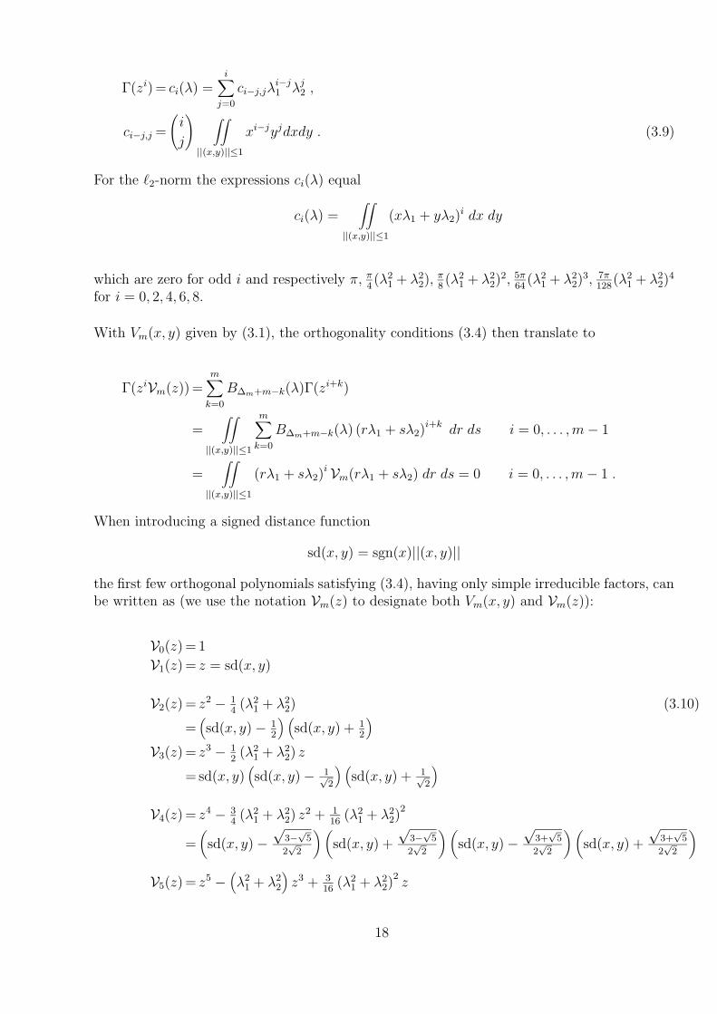
For the `2-norm the expressions ci(λ) equal
ci(λ) =∫∫
||(x,y)||≤1
(xλ1 + yλ2)i dx dy
which are zero for odd i and respectively π, π4(λ2
1 + λ22),
π8(λ2
1 + λ22)
2, 5π64
(λ21 + λ2
2)3, 7π
128(λ2
1 + λ22)
4
for i = 0, 2, 4, 6, 8.
With Vm(x, y) given by (3.1), the orthogonality conditions (3.4) then translate to
Γ(ziVm(z)) =m∑
k=0
B∆m+m−k(λ)Γ(zi+k)
=∫∫
||(x,y)||≤1
m∑
k=0
B∆m+m−k(λ) (rλ1 + sλ2)i+k dr ds i = 0, . . . ,m− 1
=∫∫
||(x,y)||≤1
(rλ1 + sλ2)i Vm(rλ1 + sλ2) dr ds = 0 i = 0, . . . ,m− 1 .
When introducing a signed distance function
sd(x, y) = sgn(x)||(x, y)||
the first few orthogonal polynomials satisfying (3.4), having only simple irreducible factors, canbe written as (we use the notation Vm(z) to designate both Vm(x, y) and Vm(z)):
V0(z) = 1
V1(z) = z = sd(x, y)
V2(z) = z2 − 14(λ2
1 + λ22) (3.10)
=(sd(x, y) − 1
2
) (sd(x, y) + 1
2
)
V3(z) = z3 − 12(λ2
1 + λ22) z
= sd(x, y)(sd(x, y) − 1√
2
) (sd(x, y) + 1√
2
)
V4(z) = z4 − 34(λ2
1 + λ22) z
2 + 116
(λ21 + λ2
2)2
=(sd(x, y) −
√3−
√5
2√
2
)(sd(x, y) +
√3−
√5
2√
2
)(sd(x, y) −
√3+
√5
2√
2
)(sd(x, y) +
√3+
√5
2√
2
)
V5(z) = z5 −(λ2
1 + λ22
)z3 + 3
16(λ2
1 + λ22)
2z
18

= sd(x, y)(sd(x, y) − 1
2
) (sd(x, y) + 1
2
) (sd(x, y) −
√3
2
) (sd(x, y) +
√3
2
).
Let us now fix λ = λ∗ and take a look at the projected functions
fλ∗(z) = f(λ∗1z, λ
∗2z),
Vm,λ∗(z) =Vm(λ∗1z, λ∗2z),
Wm,λ∗(z) =Wm(λ∗1z, λ∗2z).
If we introduce the linear functional c∗ acting on the variable z, as
c∗(zi) = ci(λ∗) = Γ(zi) |λ=λ∗ (3.11)
then we can prove the following projection property of the Vm(x, y).
In the following result we use the notation Vm(z) to denote the univariate polynomials ofdegree m orthogonal with respect to the linear functional c∗. The reader should not confusethese polynomials with the Vm(z) or the Vm(x, y).
Theorem 3.5 Let the monic univariate polynomials Vm(z) satisfy the orthogonality conditions
c∗(ziVm(z)) = 0 i = 0, . . . ,m− 1 .
with c∗ given by (3.11), and let the polynomials Vm(x, y) = Vm(z) satisfy the orthogonalityconditions (3.4). Then
Hm(λ∗1, λ∗2)Vm(z) = pm(λ∗1, λ
∗2)Vm,λ∗(z)
= pm(λ∗1, λ∗2)Vm(λ∗1z, λ
∗2z).
If the functional Γ is positive definite, then the zeroes z(m)i (λ∗) of Vm,λ∗(z) are real and simple
because the functional c∗ is positive definite. Then according to the implicit function theorem,there exists for each z
(m)i (λ∗) a unique holomorphic function φ
(m)i (λ∗1, λ
∗2) such that in a neigh-
borhood of z(m)i (λ∗),
Vm(z) = 0 ⇐⇒ z = φ(m)i (λ∗1, λ
∗2).
Since this is true for each λ = λ∗ because Γ is positive definite, this implies that for eachi = 1, . . . ,m the zeroes z
(m)i can be viewed as a holomorphic function of λ, namely z
(m)i =
φ(m)i (λ1, λ2). Let us denote
A(m)i (λ) =
Wm,λ(z(m)i )
V ′m,λ(z
(m)i )
=Wm(φ
(m)i (λ))
V ′m(φ
(m)i (λ))
.
19

Then the following cubature formula can rightfully be called a Gaussian cubature formula. Theproof of this fact can be found in [5].
Theorem 3.6 Let P(z) be a polynomial of degree 2m− 1 belonging to C(λ1, λ2)[z], the set ofpolynomials in the variable z with coefficients from the space of bivariate rational functions inλ1 and λ2 with complex coefficients. Let the functions φ
(m)i (λ1, λ2) be given as above and be such
that
∀λ ∈ S2 : j 6= i =⇒ φ(m)j (λ) 6= φ
(m)i (λ).
Then for z = λ1x+ λ2y holds
∫∫
||(x,y)||≤1
P(λ1x+ λ2y)dxdy =m∑
i=1
A(m)i (λ)P(φ
(m)i (λ)).
Let us illustrate Theorem 3.6 with an example. Take
P(z) = P(λ1x+ λ2y) =3∑
i=0
(3
i
)(λ1
λ2
)3−i
(λ1x+ λ2y)i
and consider again the `2-norm. Then
∫∫
||(x,y)||≤1
P(λ1x+ λ2y)dx dy =πλ1
4λ32
(4λ21 + 3λ2
1λ22 + 3λ4
2). (3.12)
The exact integration rule given in Theorem 3.6, applies to (3.12) with m = 2. From theorthogonal function V2(x, y) = V2(z) given in (3.10), we obtain the zeroes
φ(2)1 (λ) =
1
2
√λ2
1 + λ22
φ(2)2 (λ) =−1
2
√λ2
1 + λ22
and the weights
A(2)1 (λ) = A
(2)2 (λ) =
π
2.
The integration ruleA
(2)1 P(φ
(2)1 (λ)) + A
(2)2 P(φ
(2)2 (λ))
then yields the same result as (3.12). In fact, the Gaussian m-point cubature formula given inTheorem 3.6 exactly integrates a parameterized family of polynomials, over a domain in R
2,or more generally R
n. The m nodes and weights are themselves functions of the parameters λ1
and λ2.
For the `1- and `∞-norm similar computations can be performed: after obtaining the ci(λ) forthese norms, the orthogonal polynomial V2(z) constructed from the ci(λ) delivers all necessaryingredients for the application of the Gaussian cubature rule.
20

More properties of the homogeneous orthogonal polynomials Vm(x, y) can be proved, such as thefact that they are the characteristic polynomials of certain parametrized tridiagonal matrices [7].The connection between their theory and the theory of the univariate orthogonal polynomialsis very close.
4 Vector and matrix orthogonal polynomials
In this section, we generalize some results of Section 1 on scalar orthogonal polynomials to thevector and matrix case.
Let Πα be the space of all vector polynomials with α components. Let Πα~n be the subspace of
Πα of all vector polynomials of degree (elementwise) at most ~n ∈ Nα. The dimension of this
subspace is
|~n| =α∑
i=1
(ni + 1) with ~n = (n1, n2, . . . , nα).
Following the notation of Section 1, we denote a set of basis functions for Πα~n as
{B1, B2, . . . , B|~n|}.
In contrast to the scalar case, a nested basis of increasing degree can be chosen in severaldifferent ways, e.g., with α = 2, a natural choice could be
1
0
,
0
1
,
x
0
,
0
x
, . . . . (4.1)
Another possibility is
1
0
,
x
0
,
x2
0
,
0
1
,
x3
0
,
0
x
, . . . .
Once, we have chosen a (nested) basis in Πα~n, each element of Πα
~n can be identified by anelement of C
|~n|×1. Similarly, choosing a basis in the dual space, each linear functional on Πα~n
can be represented by an element of C1×|~n|.
Let µ be a matrix-valued measure of a finite or infinite interval I on the real line. Then, thecomponents of
Lk(P ) =∫
I
xkdµ(x)P (x)
can be considered as the duals of the vector polynomials
xk
0...
0
,
0
xk
...
0
, . . .
21

The corresponding inner product for two vector polynomials P and Q is introduced as follows
〈Q,P 〉 =∞∑
k=0
∞∑
l=0
qTk 〈xkIα, x
lIα〉pl =∞∑
k=0
qTk Ll(P )
with Q(x) =∑∞
k=0 qkxk and P (x) =
∑∞k=0 pkx
k. When we consider the natural nested basis(4.1), the moment matrix is block Hankel and all blocks are completely determined by thematrix-valued function L defined as
L(xi) =∫
I
xidµ(x)
because the (k, l)th block of the moment matrix equals
Lk(xl) = L(xk+l).
In a similar way, we can extend the results for scalar polynomials orthogonal on the unitcircle into vector orthogonal polynomials where, then, the moment matrix has a block Toeplitzstructure.
Taking the natural nested basis, and taking the vector orthogonal polynomials together ingroups of α elements, we derive α×αmatrix orthogonal polynomials Pi, i = 0, 1, . . . of increasingdegree i satisfying the “matrix” orthogonality relationship
⟨Pi, Pj
⟩= δijIα
with 〈·, ·〉 defined in an obvious way based on the inner product of vector polynomials. Sev-eral other properties of Section 1 can be generalized in the same way for vector and matrixorthogonal polynomials [44,42,43].
Let us consider the following discrete inner product based on the points zi ∈ C, i = 1, 2, . . . , Nand the weights (vectors) Fi ∈ C
α×1:
〈V, U〉 =N∑
i=1
V (zi)HFiF
Hi U(zi), with U, V ∈ Πα
~n.
Note that this is a true inner product as long as there is no element U from Πα~n such that
〈U,U〉 = 0. To find a recurrence relation for the vector orthogonal polynomials based on thenatural nested basis for Πα
~n, we can solve the following inverse eigenvalue problem. Given zi, Fi,i = 1, 2, . . . , N , find the upper triangular matrix R and the generalized Hessenberg matrix Hsuch that
[QHF |QHΛzQ
]=[R|H
], (4.2)
where the right-hand side matrix has upper triangular structure, the rows of the matrix F arethe weights FH
i , the matrix Q is a unitary N ×N matrix, Λz is the diagonal matrix with thepoints zi on the diagonal, and R is a N × α matrix which is zero except for the upper α × αblock which is the upper triangular matrix R. Note that because H =
[R|H
]has the upper
triangular structure, H is a generalized Hessenberg matrix having α subdiagonals different from
22

zero. Instead of the natural nested basis, we can take a more complicated nested basis. In thiscase the matrix
[R|H
]will still have the upper triangular structure, but only after a column
permutation.
The columns of the unitary matrix Q are connected to the values of the corresponding vectororthogonal polynomials φ1, φ2, . . . as follows
Qij = FHi φj(zi), with i, j = 1, 2, . . . , N.
Because the relation (4.2) gives us a recurrence for the columns of Q, we get the correspondingrecurrence relation for the vector orthogonal polynomials φi:
hiiφi(z) = ei −i−1∑
j=1
hjihjiφj(z), i = 1, 2, . . . , α
= zφi−α −i−1∑
j=1
hjihjiφj(z), i = α + 1, α + 2, . . . , N
where hij is the (i, j)th element of the upper triangular (rectangular) matrix H.
For zi arbitrary chosen in the complex plane, the previous inverse eigenvalue problem requiresO(N 3) floating point operations. However, this computational complexity decreases by an orderof magnitude in the following two special cases.
(1) All the points zi are real and the weights are real vectors
In this case, all computations can be done using real numbers. Hence, the matrix Q will alsobe real (orthogonal). Therefore, H = QTZQ will be symmetric and because H is a gener-alized Hessenberg, it will be a symmetric banded matrix with bandwidth 2α + 1. Note thatthe recurrence relation for the vector orthogonal polynomials only involves 2α + 1 of thesepolynomials, i.e., for the special case of α = 1, we obtain the classical 3-term recurrencerelation.
(2) All the points zi are on the unit circle
In this case, H is not only generalized Hessenberg but also unitary. In this case, the matrixH can be written as a product of more simple unitary matrices Gi:
H = G1G2 · · ·GN−α
where Gi = Ii−1 ⊕ Qi ⊕ IN−i−α−1 with Qi an α × α unitary matrix. When the inverseeigenvalue problem is solved where H is parameterized in terms of the unitary matricesQi, the computational complexity reduces to O(N 2). The recurrence relation for the vectororthonormal polynomials turns out to be a generalization of the classical Szego relation.
For more details on vector orthogonal polynomials with respect to a discrete inner product, werefer the interested reader to [17,51,53]. These vector and/or matrix orthogonal polynomialscan be applied in system identification [40,18], to design fast and accurate algorithms to solvestructured systems [52,54].
23

5 Multiple orthogonality and Hermite-Pade approximation
Hermite-Pade approximation is simultaneous rational approximation to a vector of r functionsf1, f2, . . . , fr, which are all given as Taylor series around a point a ∈ C and for which werequire interpolation conditions at a. We will restrict our attention to Hermite-Pade approx-imation around infinity and impose interpolation conditions at infinity. Certain polynomialswhich appear in this rational approximation problem satisfy a number of orthogonality condi-tions with respect to r measures and hence we call them multiple orthogonal polynomials. Thesepolynomials are one-variable polynomials but the degree is a multi-index. A good source forinformation on Hermite-Pade approximation is the book by Nikishin and Sorokin [38, Chapter4], where the multiple orthogonal polynomials are called polyorthogonal polynomials. Othergood sources of information are the surveys by Aptekarev [2] and de Bruin [21].
Suppose we are given r functions with Laurent expansions
fj(z) =∞∑
k=0
ck,j
zk+1, j = 1, 2, . . . , r.
There are basically two different types of Hermite-Pade approximation. First we will needmulti-indices ~n = (n1, n2, . . . , nr) ∈ N
r and their size |~n| = n1 + n2 + · · · + nr.
Definition 5.1 (Type I) Type I Hermite-Pade approximation to the vector (f1, . . . , fr) nearinfinity consists of finding a vector of polynomials (A~n,1, . . . , A~n,r) and a polynomial B~n, withA~n,j of degree ≤ nj − 1, such that
r∑
j=1
A~n,j(z)fj(z) −B~n(z) = O(
1
z|~n|
), z → ∞. (5.1)
In type I Hermite-Pade approximation one wants to approximate a linear combination (withpolynomial coefficients) of the r functions by a polynomial. This is often done for the vector offunctions f, f 2, . . . , f r, where f is a given function. The solution of the equation
r∑
j=1
A~n,j(z)fj(z) −B~n(z) = 0
is an algebraic function and then gives an algebraic approximant f for the function f .
Definition 5.2 (Type II) Type II Hermite-Pade approximation to the vector (f1, . . . , fr) nearinfinity consists of finding a polynomial P~n of degree ≤ |~n| and polynomials Q~n,j (j = 1, 2, . . . , r)such that
P~n(z)f1(z) −Q~n,1(z) =O(
1
zn1+1
), z → ∞
... (5.2)
24

P~n(z)fr(z) −Q~n,r(z) =O(
1
znr+1
), z → ∞.
Type II Hermite-Pade approximation therefore corresponds to an approximation of each func-tion fj separately by rational functions with a common denominator P~n. Combinations of typeI and type II Hermite-Pade approximation also are possible.
5.1 Orthogonality
When we consider r Markov functions
fj(z) =
bj∫
aj
dµj(x)
z − x, j = 1, 2, . . . , r,
then Hermite-Pade approximation corresponds to certain orthogonality conditions.
First consider type I approximation. Multiply (5.1) by zk and integrate over a contour Γ en-circling all the intervals [aj, bj] in the positive direction, then
1
2πi
∫
Γ
r∑
j=1
zkA~n,j(z)fj(z) dz −1
2πi
∫
Γ
zkB~n(z) dz =∞∑
`=|~n|b`
1
2πi
∫
Γ
zk−` dz.
Clearly Cauchy’s theorem implies
1
2πi
∫
Γ
zkB~n(z) dz = 0.
Furthermore, there is only a contribution on the right hand side when ` = k + 1, so whenk ≤ |~n| − 2, then none of the terms in the infinite sum have a contribution. Therefore we seethat
1
2πi
∫
Γ
r∑
j=1
zkA~n,j(z)fj(z) dz = 0, 0 ≤ k ≤ |~n| − 2.
Now each fj is a Markov function, so by changing the order of integration we get
1
2πi
∫
Γ
zkA~n,j(z)fj(z) dz =
bj∫
aj
dµj(x)1
2πi
∫
Γ
zkA~n,j(z)
z − xdz.
25
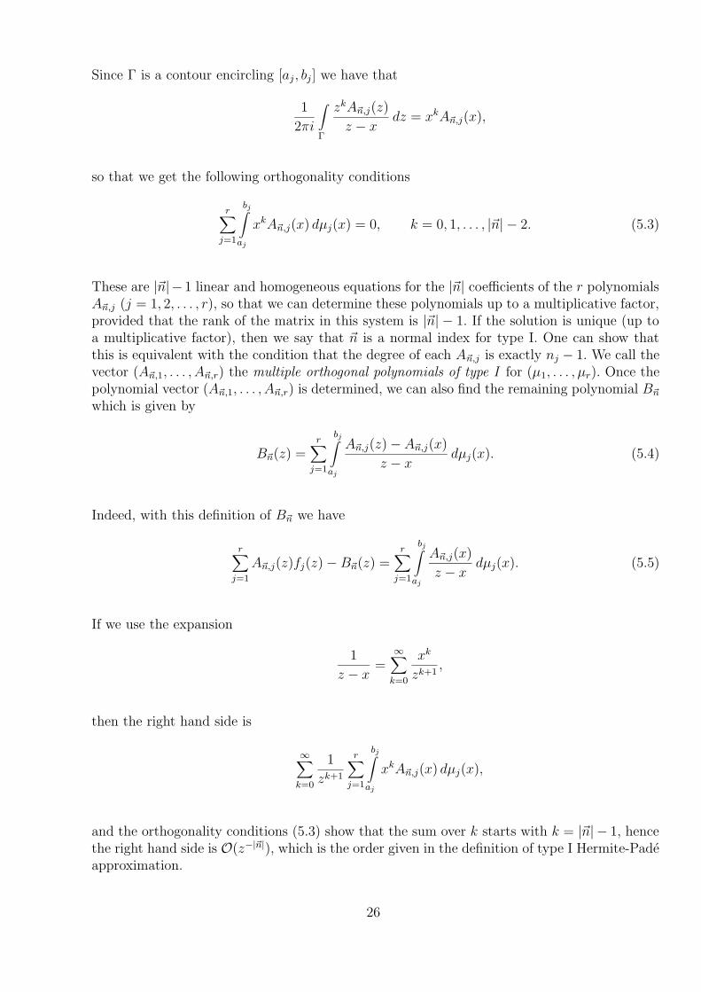
Since Γ is a contour encircling [aj, bj] we have that
1
2πi
∫
Γ
zkA~n,j(z)
z − xdz = xkA~n,j(x),
so that we get the following orthogonality conditions
r∑
j=1
bj∫
aj
xkA~n,j(x) dµj(x) = 0, k = 0, 1, . . . , |~n| − 2. (5.3)
These are |~n|− 1 linear and homogeneous equations for the |~n| coefficients of the r polynomialsA~n,j (j = 1, 2, . . . , r), so that we can determine these polynomials up to a multiplicative factor,provided that the rank of the matrix in this system is |~n| − 1. If the solution is unique (up toa multiplicative factor), then we say that ~n is a normal index for type I. One can show thatthis is equivalent with the condition that the degree of each A~n,j is exactly nj − 1. We call thevector (A~n,1, . . . , A~n,r) the multiple orthogonal polynomials of type I for (µ1, . . . , µr). Once thepolynomial vector (A~n,1, . . . , A~n,r) is determined, we can also find the remaining polynomial B~n
which is given by
B~n(z) =r∑
j=1
bj∫
aj
A~n,j(z) − A~n,j(x)
z − xdµj(x). (5.4)
Indeed, with this definition of B~n we have
r∑
j=1
A~n,j(z)fj(z) −B~n(z) =r∑
j=1
bj∫
aj
A~n,j(x)
z − xdµj(x). (5.5)
If we use the expansion
1
z − x=
∞∑
k=0
xk
zk+1,
then the right hand side is
∞∑
k=0
1
zk+1
r∑
j=1
bj∫
aj
xkA~n,j(x) dµj(x),
and the orthogonality conditions (5.3) show that the sum over k starts with k = |~n| − 1, hencethe right hand side is O(z−|~n|), which is the order given in the definition of type I Hermite-Padeapproximation.
26

Next we consider type II approximation. Multiply (5.2) by zk and integrate over a contour Γencircling all the intervals [aj, bj], then
1
2πi
∫
Γ
zkP~n(z)fj(z) dz −1
2πi
∫
Γ
zkQ~n,j(z) dz =∞∑
`=nj+1
b`1
2πi
∫
Γ
zk−` dz.
Cauchy’s theorem gives
1
2πi
∫
Γ
zkQ~n,j(z) dz = 0,
and on the right hand side we only have a contribution when ` = k+ 1. So for k ≤ nj − 1 noneof the terms in the infinite sum contribute. Hence
1
2πi
∫
Γ
zkP~n(z)fj(z) dz = 0, 0 ≤ k ≤ nj − 1.
Interchanging the order of integration on the left hand side gives the orthogonality conditions
b1∫
a1
xkP~n(x) dµ1(x) = 0, k = 0, 1, . . . , n1 − 1,
... (5.6)br∫
ar
xkP~n(x) dµr(x) = 0, k = 0, 1, . . . , nr − 1.
This gives |~n| linear and homogeneous equations for the |~n|+ 1 coefficients of P~n, hence we canobtain the polynomial P~n up to a multiplicative factor, provided the matrix of coefficients hasrank |~n|. In that case we call the index ~n normal for type II. One can show that this is equivalentwith the condition that the degree of P~n is exactly |~n|. We call this polynomial P~n the multipleorthogonal polynomial of type II for (µ1, . . . , µr). Once the polynomial P~n is determined, wecan obtain the polynomials Q~n,j by
Q~n,j(z) =
bj∫
aj
P~n(z) − P~n(x)
z − xdµj(x). (5.7)
Indeed, with this expression for Q~n,j we have
P~n(z)fj(z) −Q~n,j(z) =
bj∫
aj
P~n(x)
z − xdµj(x), (5.8)
27
and if we expand 1/(z − x), then the right hand side is of the form
∞∑
k=0
1
zk+1
bj∫
aj
xkP~n(x) dµj(x),
and the orthogonality conditions (5.6) show that the infinite sum starts at k = nj, whichgives an expression of O(z−nj−1), which is exactly what is required for type II Hermite-Padeapproximation.
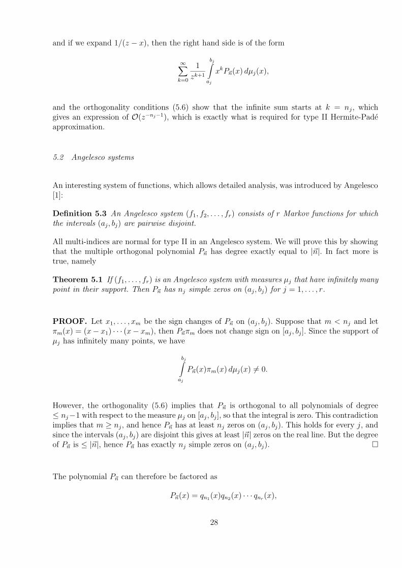
5.2 Angelesco systems
An interesting system of functions, which allows detailed analysis, was introduced by Angelesco[1]:
Definition 5.3 An Angelesco system (f1, f2, . . . , fr) consists of r Markov functions for whichthe intervals (aj, bj) are pairwise disjoint.
All multi-indices are normal for type II in an Angelesco system. We will prove this by showingthat the multiple orthogonal polynomial P~n has degree exactly equal to |~n|. In fact more istrue, namely
Theorem 5.1 If (f1, . . . , fr) is an Angelesco system with measures µj that have infinitely manypoint in their support. Then P~n has nj simple zeros on (aj, bj) for j = 1, . . . , r.
PROOF. Let x1, . . . , xm be the sign changes of P~n on (aj, bj). Suppose that m < nj and letπm(x) = (x− x1) · · · (x− xm), then P~nπm does not change sign on [aj, bj]. Since the support ofµj has infinitely many points, we have
bj∫
aj
P~n(x)πm(x) dµj(x) 6= 0.
However, the orthogonality (5.6) implies that P~n is orthogonal to all polynomials of degree≤ nj−1 with respect to the measure µj on [aj, bj], so that the integral is zero. This contradictionimplies that m ≥ nj, and hence P~n has at least nj zeros on (aj, bj). This holds for every j, andsince the intervals (aj, bj) are disjoint this gives at least |~n| zeros on the real line. But the degreeof P~n is ≤ |~n|, hence P~n has exactly nj simple zeros on (aj, bj). �
The polynomial P~n can therefore be factored as
P~n(x) = qn1(x)qn2
(x) · · · qnr(x),
28

where each qnjis a polynomial of degree nj with its zeros on (aj, bj). The orthogonality (5.6)
then gives
bj∫
aj
xkqnj(x)
∏
i6=j
qni(x) dµj(x) = 0, k = 0, 1, . . . , nj − 1. (5.9)
The product∏
i6=j qni(x) does not change sign on (aj, bj), hence (5.9) shows that qnj
is anordinary orthogonal polynomial of degree nj on the interval [aj, bj] with respect to the measure∏
i6=j |qni(x)| dµj(x). The measure depends on the multi-index ~n.
5.3 Algebraic Chebyshev systems
A Chebyshev system {ϕ1, . . . , ϕn} on [a, b] is a system of n linearly independent functions suchthat every linear combination
∑nk=1 akϕk has at most n − 1 zeros on [a, b]. This is equivalent
with the condition that
det
ϕ1(x1) ϕ1(x2) · · · ϕ1(xn)
ϕ2(x1) ϕ2(x2) · · · ϕ2(xn)...
... · · · ...
ϕn(x1) ϕn(x2) · · · ϕn(xn)
6= 0
for every choice of n different points x1, . . . , xn ∈ [a, b]. Indeed, when x1, . . . , xn are such thatthe determinant is zero, then there is a linear combination of the rows that gives a zero row, butthis means that for this linear combination
∑nk=1 akϕk has zeros at x1, . . . , xn, giving n zeros,
which is not allowed.
Definition 5.4 A system (f1, . . . , fr) is an algebraic Chebyshev system (AT system) for theindex ~n if each fj is a Markov function on the same interval [a, b] with a measure wj(x) dµ(x),where µ has an infinite support and the wj are such that
{w1, xw1, . . . , xn1−1w1, w2, xw2, . . . , x
n2−1w2, . . . , wr, xwr, . . . , xnr−1wr} (5.10)
is a Chebyshev system on [a, b].
Theorem 5.2 Suppose ~n is a multi-index such that (f1, . . . , fr) is an AT system on [a, b] forevery index ~m for which mj ≤ nj (1 ≤ j ≤ r). Then P~n has |~n| zeros on (a, b) and hence ~n isa normal index for type II.
PROOF. Let x1, . . . , xm be the sign changes of P~n on (a, b) and suppose that m < |~n|. We canthen find a multi-index ~m such that |~m| = m and mj ≤ nj for every 1 ≤ j ≤ r and mk < nk
29

for some 1 ≤ k ≤ r. Consider the interpolation problem where we want to find a function
L(x) =r∑
j=1
qj(x)wj(x),
where qj is a polynomial of degree mj − 1 if j 6= k and qk a polynomial of degree mk, thatsatisfies
L(xj) = 0, j = 1, ...,m,
L(x0) = 1, for some other point x0 ∈ [a, b],
then this interpolation problem has a unique solution since this involves a Chebyshev systemof basis functions. The function L has, by construction, m zeros and the Chebyshev system hasm + 1 basis functions, so L can have at most m zeros on [a, b] and each zero is a sign change.Hence P~nL does not change sign on [a, b]. Since µ has infinite support, we thus have
b∫
a
L(x)P~n(x)dµ(x) 6= 0.
But the orthogonality (5.6) gives
b∫
a
qj(x)P~n(x)wj(x) dµ(x) = 0, j = 1, 2, . . . , r,
and this contradiction implies that P~n has |~n| simple zeros on (a, b). �
We have a similar result for type I Hermite-Pade approximation:
Theorem 5.3 Suppose ~n is a multi-index such that (f1, . . . , fr) is an AT system on [a, b] forevery index ~m for which mj ≤ nj (1 ≤ j ≤ r). Then
∑rj=1A~n,jwj has |~n|− 1 zeros on (a, b) and
~n is a normal index for type I.
PROOF. Let x1, . . . , xm be the sign changes of∑r
j=1A~n,jwj on (a, b) and suppose that m <|~n| − 1. Let πm be the monic polynomial with these points as zeros, then πm
∑rj=1A~n,jwj does
not change sign on [a, b] and hence
b∫
a
πm(x)r∑
j=1
A~n,j(x)wj(x) dµ(x) 6= 0.
But the orthogonality conditions (5.3) indicate that this integral is zero. This contradictionimplies that m ≥ |~n| − 1. The sum
∑rj=1A~n,jwj is a linear combination of the Chebyshev
system (5.10), hence it has at most |~n| − 1 zeros on [a, b]. Therefore we see that m = |~n| − 1.
30

To see that the index ~n is normal for type I, we assume that for some k with 1 ≤ k ≤ r thedegree of A~n,k is less than nk − 1. Then
∑rj=1A~n,jwj is a linear combination of a the Chebyshev
system (5.10) from which the function xnk−1wk is removed. This is still a Chebyshev systemby assumption, and hence this linear combination has at most |~n| − 2 zeros on [a, b]. But thiscontradicts our previous observation that it has |~n| − 1 zeros. Therefore every A~n,j has degreeexactly nj − 1, so that the index ~n is normal. �
5.4 Nikishin systems
A special construction, suggested by Nikishin [39], gives an AT system that can be handledin some detail. The construction is by induction. A Nikishin system of order 1 is a Markovfunction f1,1 for a measure µ1 on the interval [a1, b1]. A Nikishin system of order 2 is a vectorof Markov functions (f1,2, f2,2) on [a2, b2] such that
f1,2(z) =
b2∫
a2
dµ2(x)
z − x, f2,2(z) =
b2∫
a2
f1,1(x)dµ2(x)
z − x,
where f1,1 is a Nikishin system of order 1 on [a1, b1] and (a1, b1) ∩ (a2, b2) = ∅. In general wehave
Definition 5.5 A Nikishin system of order r consists of r Markov functions (f1,r, . . . , fr,r) on[ar, br] such that
f1,r(z) =
br∫
ar
dµr(x)
z − x, (5.11)
fj,r(z) =
br∫
ar
fj−1,r−1(x)dµr(x)
z − x, j = 2, . . . , r, (5.12)
where (f1,r−1, . . . , fr−1,r−1) is a Nikishin system of order r − 1 on [ar−1, br−1] and (ar, br) ∩(ar−1, br−1) = ∅.
For a Nikishin system of order r one knows that the multi-indices ~n with n1 ≥ n2 ≥ · · · ≥ nr
are normal (the system is an AT-system for these indices), but is an open problem whetherevery multi-index is normal (for r > 2; for r = 2 it has been proved that every multi-index isnormal).
What can be said about type II Hermite-Pade approximation for r = 2? Recall (5.8) for thefunction f1,2:
Pn1,n2(y)f1,2(y) −Qn1,n2;1(y) =
b2∫
a2
Pn1,n2(x)
y − xdµ2(x).
31

Multiply both sides by yk, with k ≤ n1, then the right hand side is
b2∫
a2
ykPn1,n2(x)
y − xdµ2(x) =
b2∫
a2
(yk − xk)Pn1,n2(x)
y − xdµ2(x) +
b2∫
a2
xkPn1,n2(x)
y − xdµ2(x).
Clearly (yk − xk)/(y − x) is a polynomial in x of degree k − 1 ≤ n1 − 1 hence the first integralon the right vanishes because of the orthogonality (5.6). Integrate over the variable y ∈ [a1, b1]with respect to the measure µ1, then we find for k ≤ n1
b1∫
a1
[Pn1,n2(y)f1,2(y) −Qn1,n2;1(y)]y
k dµ1(y) =
b1∫
a1
b2∫
a2
xkPn1,n2(x)
y − xdµ2(x) dµ1(y).
Change the order of integration on the right hand side, then
b1∫
a1
[Pn1,n2(y)f1,2(y) −Qn1,n2;1(y)]y
k dµ1(y) = −b2∫
a2
xkPn1,n2(x)f1,1(x) dµ2(x)
and this is zero for k ≤ n2 − 1. Hence if n2 ≤ n1 + 1 then the expression Pn1,n2(y)f1,2(y) −
Qn1,n2;1(y) is orthogonal to all polynomials of degree ≤ n2 − 1 on [a1, b1]. This implies thatPn1,n2
(y)f1,2(y)−Qn1,n2;1(y) has at least n2 zeros on (a1, b1) using an argument similar to whatwe have been using earlier. Let Rn2
be the monic polynomial with n2 of these zeros on (a1, b1),then [Pn1,n2
(y)f1,2(y)−Qn1,n2;1(y)]/Rn2(y) is an analytic function on C \ [a2, b2], which has the
representation
Pn1,n2(y)f1,2(y) −Qn1,n2;1(y)
Rn2(y)
=1
Rn2(y)
b2∫
a2
Pn1,n2(x)
y − xdµ2(x).
Multiply both sides by yk and integrate over a contour Γ encircling the interval [a2, b2] in thepositive direction, but with all the zeros of Rn2
outside Γ, then
1
2πi
∫
Γ
ykPn1,n2(y)f1,2(y) −Qn1,n2;1(y)
Rn2(y)
dy =1
2πi
∫
Γ
yk
Rn2(y)
Pn1,n2(x)
y − xdµ2(x) dy.
If we interchange the order of integration on the right hand side and use Cauchy’s theorem,then this gives the integral
b2∫
a2
xkPn1,n2(x)
dµ2(x)
Rn2(x)
.
By the interpolation condition (5.2) the integrand on the left hand side is of the order O(yk−n1−n2−1),so if we use Cauchy’s theorem for the exterior of Γ, then the integral vanishes for k ≤ n1+n2−1.
32
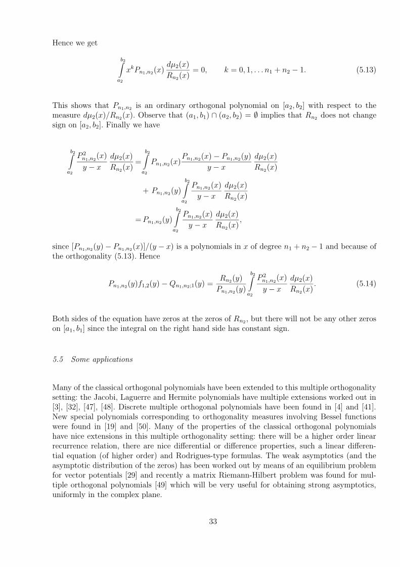
Hence we get
b2∫
a2
xkPn1,n2(x)
dµ2(x)
Rn2(x)
= 0, k = 0, 1, . . . n1 + n2 − 1. (5.13)
This shows that Pn1,n2is an ordinary orthogonal polynomial on [a2, b2] with respect to the
measure dµ2(x)/Rn2(x). Observe that (a1, b1) ∩ (a2, b2) = ∅ implies that Rn2
does not changesign on [a2, b2]. Finally we have
b2∫
a2
P 2n1,n2
(x)
y − x
dµ2(x)
Rn2(x)
=
b2∫
a2
Pn1,n2(x)
Pn1,n2(x) − Pn1,n2
(y)
y − x
dµ2(x)
Rn2(x)
+ Pn1,n2(y)
b2∫
a2
Pn1,n2(x)
y − x
dµ2(x)
Rn2(x)
=Pn1,n2(y)
b2∫
a2
Pn1,n2(x)
y − x
dµ2(x)
Rn2(x)
,
since [Pn1,n2(y) − Pn1,n2
(x)]/(y − x) is a polynomials in x of degree n1 + n2 − 1 and because ofthe orthogonality (5.13). Hence
Pn1,n2(y)f1,2(y) −Qn1,n2;1(y) =
Rn2(y)
Pn1,n2(y)
b2∫
a2
P 2n1,n2
(x)
y − x
dµ2(x)
Rn2(x)
. (5.14)
Both sides of the equation have zeros at the zeros of Rn2, but there will not be any other zeros
on [a1, b1] since the integral on the right hand side has constant sign.
5.5 Some applications
Many of the classical orthogonal polynomials have been extended to this multiple orthogonalitysetting: the Jacobi, Laguerre and Hermite polynomials have multiple extensions worked out in[3], [32], [47], [48]. Discrete multiple orthogonal polynomials have been found in [4] and [41].New special polynomials corresponding to orthogonality measures involving Bessel functionswere found in [19] and [50]. Many of the properties of the classical orthogonal polynomialshave nice extensions in this multiple orthogonality setting: there will be a higher order linearrecurrence relation, there are nice differential or difference properties, such a linear differen-tial equation (of higher order) and Rodrigues-type formulas. The weak asymptotics (and theasymptotic distribution of the zeros) has been worked out by means of an equilibrium problemfor vector potentials [29] and recently a matrix Riemann-Hilbert problem was found for mul-tiple orthogonal polynomials [49] which will be very useful for obtaining strong asymptotics,uniformly in the complex plane.
33

5.5.1 Irrationality and transcendence
Hermite-Pade approximation finds its origin in number theory. Hermite’s proof of the tran-scendence of e is based on Hermite-Pade approximation of (ex, e2x, . . . , erx) at x = 0. Manyproofs of irrationality are also based on Hermite-Pade approximation, even though this is oftennot explicit in the proof. Apery’s proof that ζ(3) is irrational can be reduced to Hermite-Padeapproximation to three functions
f1(z) =
1∫
0
dx
z − x, f2(z) = −
1∫
0
log xdx
z − x, f3(z) =
1
2
1∫
0
log2 xdx
z − x,
which form an AT-system. The proof uses a mixture of type I and type II Hermite-Padeapproximation: find polynomials (An, Bn) (both of degree n) and polynomials Cn and Dn suchthat
An(1) = 0
An(z)f1(z) +Bn(z)f2(z) − Cn(z) =O(1/zn+1), z → ∞An(z)f2(z) + 2Bn(z)f3(z) −Dn(z) =O(1/zn+1), z → ∞.
Observe that f3(1) = ζ(3), hence if we evaluate the approximations at z = 1, then we see that2Bn(1)ζ(3)−Dn(1) will be small and Dn(1)/(2Bn(1)) is a good rational approximation to ζ(3).In fact, asymptotic analysis of the error and of the denominator Bn(1) and some simple numbertheory show that this rational approximation is better than order 1, which implies that ζ(3) isirrational. See [47] for details.
For another example we consider the two Markov functions
f1(z) =
1∫
0
dx
z − x, f2(z) =
0∫
−1
dx
z − x,
which form an Angelesco system. Some straightforward calculus gives
f1(i) = −1
2log 2 − iπ
4, f2(i) =
1
2log 2 − iπ
4,
hence the sum gives f1(i) + f2(i) = −iπ/2. The type II Hermite-Pade approximants for f1 andf2 will give approximations to π. Recall that
Pn,n(z)f1(z) −Qn,n;1(z) =
1∫
0
Pn,n(x)
z − xdx
Pn,n(z)f2(z) −Qn,n;2(z) =
0∫
−1
Pn,n(x)
z − xdx.
34

Summing both equations gives
Pn,n(z)[f1(z) + f2(z)] − [Qn,n;1(z) +Qn,n;2(z)] =
1∫
−1
Pn,n(x)
z − xdx.
So the fact that we are using a common denominator comes in very handy here. Then weevaluate these expressions at z = i and hope that Pn,n(i) and Qn,n;1(i) + Qn,n;2(i) are (up tothe factor i) integers or rational numbers with simple denominators. Asymptotic propertiesof the Hermite-Pade approximants and the multiple orthogonal polynomials then gives usefulquantitative information about the order of rational approximation to π. For this particularcase the type II multiple orthogonal polynomials are given by a Rodrigues formula
Pn,n(x) =dn
dxn
(xn(1 − x2)n
),
and these polynomials are known as Legendre-Angelesco polynomials. They have been studiedin detail by Kalyagin [32] (see also [47]). The Rodrigues formula in fact simplifies the asymptoticanalysis, since integration by parts now gives
1∫
−1
Pn,n(x)
z − xdx =
1∫
−1
(−1)nn!xn(1 − x2)n
(z − x)n+1dx,
which can be handled easily. Some trial and error show that one gets better results by taking2n instead of n, and by differentiating n times extra:
rdn
dzn(P2n,2n(z)[f1(z) + f2(z)] − [Q2n,2n;1(z) +Q2n,2n;2(z)])z=i
= (3n)!(−i)n+1
1∫
−1
x2n(1 − x2)2n
(1 + ix)3n+1dx. (5.15)
This gives rational approximants to π of the form
π =bnancn
+Kn
an
,
where an, bn, cn are explicitly known integers and Kn is the integral on the right hand side of(5.15). The rational approximants show that π is irrational (which was shown already in 1761by Lambert), but they even show that you can’t approximate π by rational at order greaterthan 23.271 (Beukers [8]). This upper bound for the order of approximation can be reduced to8.02 (Hata [30]) by considering Markov functions f1 and f3, with
f3(z) =
0∫
−i
dx
z − x.
35

This f3 is now over a complex interval, and then Theorem 5.1 about the location of the zerosno longer holds, and the asymptotic behavior will have to be handled with another method.
5.5.2 Random matrices
Multiple orthogonal polynomials appear in certain problems in the theory of random matrices.The connection between eigenvalues of random matrices and orthogonal polynomials is wellknown: if we define a matrix ensemble by giving the joint probability density function for itseigenvalues as
P (x1, . . . , xN ) =N∏
i=1
f(xi)∏
1≤i<j≤N
(xi − xj)2,
then the eigenvalues density σN is given by
σn(x) =
∞∫
−∞· · ·
∞∫
−∞P (x, x2, . . . , xN) dx2 · · · dxN =
1
N
N−1∑
j=0
p2j(x),
where the pn are the orthonormal polynomials with weight function f . Furthermore the n-pointcorrelation function is given in terms of the Christoffel-Darboux kernel
N−1∑
j=0
pj(x)pj(y).
(see, e.g., [35, §19.3]). The Gaussian unitary ensemble corresponds to Hermite polynomials.
Recently a random matrix ensemble with an external source was considered by Brezin andHikami [11] and Zinn-Justin [60]. The joint probability density function of the matrix elementsof the random Hermitian matrix M is of the form
1
ZN
e−Tr(M2−AM) dM
where A is a fixed N ×N Hermitian matrix (the external source). Bleher and Kuijlaars [9] ob-served that the average characteristic polynomial PN(z) = E[det(zI−M)] can be characterizedby the property
∞∫
−∞PN(z)xke−(x2−ajx) dx = 0, k = 0, 1, . . . , Nj − 1,
where Nj is the multiplicity of the eigenvalue aj of A. This means that PN is a multipleHermite polynomial of type II with multi-index (N1, . . . , Nr) when A has r distinct eigenvaluesa1, . . . , ar with multiplicities N1, . . . , Nr respectively. These multiple Hermite polynomials were
36
investigated in [3]. The eigenvalue correlations and the eigenvalues density can be written interms of the kernel
N−1∑
k=0
Pk(x)Qk(y),
where the Qk are basically the type I multiple Hermite polynomials and the Pk are the typeII multiple Hermite polynomials. The asymptotic analysis of the eigenvalues and their correla-tions and universality questions can therefore be handled using asymptotic analysis of multipleHermite polynomials.
Another application is in the theory of coupled random matrices [23] [24] [33]. The two-matrixmodel deals with pairs of random matrices (M1,M2) which are both N×N Hermitian matriceswith joint density function
1
ZN
e−Tr(M41 +M4
2−τM1M2) dM1 dM2.
The statistical relevant quantities for the eigenvalues of M1 and M2 can be expressed in termsof biorthogonal polynomials pk and qk which satisfy
∞∫
−∞
∞∫
−∞pk(x)qj(y)e
−x4−y4+τxy dx dy = δk,j. (5.16)
Due to the symmetry we have that pk = qk. Consider the functions
wk(y) =
∞∫
−∞xke−x4+τxy dx,
then a simple integration by parts shows that
wk+3(y) =k
4wk−1(y) −
τy
4wk(y),
so that each wk is a linear combination of w0, w1, w2 with polynomial coefficients, in particular
w3k(y) = ak(y)w0(y) + bk−1(y)w1(y) + ck−1(y)w2(y)
w3k+1(y) = ak(y)w0(y) + bk(y)w1(y) + ck−1(y)w2(y)
w3k+2(y) = ak(y)w0(y) + bk(y)w1(y) + ck(y)w2(y)
where ak, bk, ck are polynomials of degree k. This means that
Qn(y) =
∞∫
−∞pj(y)e
−x4+τxy dx
37

is a linear combination of w0, w1, w2 with polynomials coefficients, in particular
Q3n(y) =An(y)w0(y) +Bn−1(y)w1(y) + Cn−1(y)w2(y)
Q3n+1(y) = An(y)w0(y) + Bn(y)w1(y) + Cn−1(y)w2(y)
Q3n+2(y) = An(y)w0(y) + Bn(y)w1(y) + Cn(y)w2(y).
It turns out that (An, Bn−1, Cn−1), (An, Bn, Cn−1), and (An, Bn, Cn) are multiple orthogonalpolynomials of type I for the densities e−x4
w0(x), e−x4
w1(x), e−x4
w2(x) with multi-indices (n+1, n, n), (n + 1, n + 1, n) and (n + 1, n + 1, n + 1) respectively, and p3n, p3n+1 and p3n+2 aremultiple orthogonal polynomials of type II with multi-indices (n, n, n), (n + 1, n, n) and (n +1, n+ 1, n) respectively. The multiple orthogonality conditions (5.3) and (5.6) then lead to thebiorthogonality (5.16). Note that w0 and w2 are positive densities but w1 changes sign at theorigin.
5.5.3 Simultaneous Gauss quadrature
In a number of applications we need to approximate several integrals of the same function,but with respect to different measures. The following example comes from [10]. Suppose thatg is the spectral distribution of light in the direction of the observer and w1, w2, w3 are weightfunctions describing the profiles for red, green and blue light. Then the integrals
2π∫
0
g(x)w1(x) dx,
2π∫
0
g(x)w2(x) dx,
2π∫
0
g(x)w3(x) dx
give the amount of light after passing through the filters for red, green and blue. In this casewe need to approximate three integrals of the same function g. We would like to use as fewfunction evaluations as possible, but the integrals should be accurate for polynomials g of degreeas high as possible. If we use Gauss quadrature with n nodes for each integral, then we require3n function evaluations and all integrals will be correct for polynomials of degree ≤ 2n− 1 (aspace of dimension 2n). This gives an efficiency of 3/2. In fact, with 3n function evaluationswe can double the dimension of the space in which the formula is exact. Consider the Markovfunctions
fj(z) =
b∫
a
wj(x) dx
z − x, j = 1, 2, 3
and the type II Hermite-Pade approximation problem
fj(z) −Qn,n,n;j(z)
Pn,n,n(z)= O(z−4n−1), z → ∞.
38

Now we can multiply by a polynomial π4n−1 of degree at most 4n − 1, and integrate alongcontour Γ encircling [a, b] in the positive direction, to obtain
b∫
a
π4n−1(x)wj(x), dx =3n∑
k=1
λk,n;jg(xk,n), j = 1, 2, 3 (5.17)
where xk,n are the zeros of Pn,n,n and λk,n;j are the residues of Qn,n,n;j/Pn,n,n at the zero xk,n:
λk,n;j =Qn,n,n;j(xk,n)
P ′n,n,n(xk,n)
.
Therefore the three integrals will be evaluated exactly by the three sums in (5.17) for polyno-mials of degree ≤ 4n − 1. The convergence is somewhat more difficult to handle, since we donot have a general result that the quadrature coefficients λk,n;j are positive. The positivity hasto be investigated separately for Angelesco and Nikishin systems.
References
[1] M.A. Angelesco. Sur deux extensions des fractions continues algebriques. C.R. Acad. Sci. Paris,18:262–263, 1919.
[2] A.I. Aptekarev. Multiple orthogonal polynomials. J. Comput. Appl. Math., 99:423–447, 1998.
[3] A.I. Aptekarev, A. Branquinho, and W. Van Assche. Multiple orthogonal polynomials for classicalweights. Trans. Amer. Math. Soc., 355(10):3887–3914, 2003.
[4] J. Arvesu, J. Coussement, and W. Van Assche. Some discrete multiple orthogonal polynomials.J. Comput. Appl. Math., 153:19–45, 2003.
[5] B. Benouahmane and A. Cuyt. Multivariate orthogonal polynomials, homogeneous Padeapproximants and Gaussian cubature. Numer. Algorithms, 24:1–15, 2000.
[6] B. Benouahmane and A. Cuyt. Properties of multivariate homogeneous orthogonal polynomials.J. Approx. Theory, 113:1–20, 2001.
[7] B. Benouahmane, A. Cuyt, and B. Verdonk. On the solution of parameterized (smallest, largestor multiple) eigenvalue problems. Technical report, University of Antwerp (UA), 2004.
[8] F. Beukers. A rational approach to π. Nieuw Arch. Wisk., 1:372–379, 2000.
[9] P.M. Bleher and A.B.J. Kuijlaars. Random matrices with external source and multiple orthogonalpolynomials. Internat. Math. Res. Notices, 4:109–129, 2004.
[10] C.F. Borges. On a class of Gauss-like quadrature rules. Numer. Math., 67:271–288, 1994.
[11] E. Brezin and S. Hikami. Level spacing of random matrices in an external source. Phys. Rev. E,58:7176–7185, 1998.
[12] C. Brezinski. A direct proof of the Christoffel-Darboux identity and its equivalence to therecurrence relationship. J. Comput. Appl. Math., 32:17–25, 1990.
39

[13] A. Bultheel, P. Gonzalez-Vera, E. Hendriksen, and O. Njastad. Numerical quadratures on the unitcircle: a survey with some new results. In M. Alfaro, A. Garcıa, C. Jagels, and F. Marcellan, editors,Orthogonal Polynomials on the Unit Circle: Theory and Applications, pages 1–20. UniversidadCarlos III de Madrid, 1994.
[14] A. Bultheel, P. Gonzalez-Vera, E. Hendriksen, and O. Njastad. Orthogonal rational functions,volume 5 of Cambridge Monographs on Applied and Computational Mathematics. CambridgeUniversity Press, 1999.
[15] A. Bultheel, P. Gonzalez-Vera, E. Hendriksen, and O. Njastad. Quadrature and orthogonal rationalfunctions. J. Comput. Appl. Math., 127(1-2):67–91, 2001. Invited paper.
[16] A. Bultheel and M. Van Barel. Formal orthogonal polynomials and Hankel/Toeplitz duality.Numer. Algorithms, 10:289–335, 1995.
[17] A. Bultheel and M. Van Barel. Vector orthogonal polynomials and least squares approximation.SIAM J. Matrix Anal. Appl., 16(3):863–885, 1995.
[18] A. Bultheel, M. Van Barel, and P. Van gucht. Orthogonal bases in discrete least squares rationalapproximation. J. Comput. Appl. Math., 2003. Accepted. Invited paper ICCAM 2002 Conference.
[19] E. Coussement and W. Van Assche. Multiple orthogonal polynomials associated with the modifiedBessel functions of the first kind. Constr. Approx., 19:237–263, 2003.
[20] A. Cuyt. How well can the concept of Pade approximant be generalized to the multivariate case.J. Comput. Appl. Math., 105:25–50, 1999.
[21] M.G. de Bruin. Simultaneous Pade approximation and orthogonality. In C. Brezinski,A. Draux, A.P. Magnus, P. Maroni, and A. Ronveaux, editors, Proc. Polynomes Orthogoneauxet Applications, Bar-le-Duc, 1984, volume 1171 of Lecture Notes in Math., pages 74–83. Springer,1985.
[22] M.M. Djrbashian. A survey on the theory of orthogonal systems and some open problems.In P. Nevai, editor, Orthogonal polynomials: Theory and practice, volume 294 of Series C:Mathematical and Physical Sciences, pages 135–146, Boston, 1990. NATO-ASI, Kluwer AcademicPublishers.
[23] N. Ercolani and K.T-R. McLaughlin. Asymptotics and integrable structures for biorthogonalpolynomials associated to a random two-matrix model. J. Phys. D, 152/153:232–268, 2001.
[24] B. Eynard and M.L. Mehta. Matrices coupled in a chain: eigenvalue correlations. J. Phys. A,31:4449–4456, 1998.
[25] G. Freud. Orthogonal polynomials. Pergamon Press, Oxford, 1971.
[26] B. Fritzsche and B. Kirstein amd A. Lasarow. Orthogonal rational matrix-valued functions onthe unit circle. Math. Nachr., 2002. To appear.
[27] B. Fritzsche and B. Kirstein amd A. Lasarow. Further aspects of the theory of orthogonal rationalmatrix-valued functions on the unit circle. Math. Nachr., 2003. Submitted.
[28] Ya. Geronimus. Polynomials orthogonal on a circle and interval. International Series ofMonographs in Pure and Applied Mathematics. Pergamon Press, Oxford, 1960.
[29] A.A. Gonchar, E.A. Rakhmanov, and V.N. Sorokin. Hermite-Pade approximants for systems ofMarkov-type functions. Math. Sb., 188:38–58, 1997. (Russian), Russian Acad. Sb. Math. 188
(1997), 671–696.
40

[30] M. Hata. Rational approximations to π and some other numbers. Acta Arith., 63(4):335–349,1993.
[31] W.B. Jones, O. Njastad, and W.J. Thron. Moment theory, orthogonal polynomials, quadratureand continued fractions associated with the unit circle. Bull. London Math. Soc., 21:113–152,1989.
[32] V.A. Kalyagin (Kaliaguine). On a class of polynomials defined by two orthogonality conditions.Math. Sb., 110:609–627, 1979. (Russian), Math. USSR Sb. 38 (1981), 563–580.
[33] A.B.J. Kuijlaars and K.T-R. McLaughlin. A Riemann-Hilbert problem for biorthogonalpolynomials, 2003. arXiv:math.CV/0310204.
[34] A. Lasarow. Aufbau einer Szego-Theorie fur rationale Matrixfunktionen. PhD thesis, UniversitatLeipzig, Fak. Mathematik Informatik, 2000.
[35] M.L. Mehta. Random Matrices (revised and enlarged second edition). Academic Press, Boston,1991.
[36] H.N. Mhaskar. Weighted polynomial approximation. World Scientific, 1996.
[37] P. Nevai. Geza Freud, orthogonal polynomials and Christoffel functions. A case study. J. Approx.Theory, 48:3–167, 1986.
[38] E.M. Nikishin and V.N. Sorokin. Rational approximation and orthogonality, volume 92 of Transl.Math. Monographs. Amer. Math. Soc., 1991.
[39] E.M. Nikisin. On simultaneous Pade approximants. Math. Sb., 113:499–519, 1980. (Russian);Math. USSR Sb. 41 (1982), 409–425.
[40] R. Pintelon, Y. Rolain, A. Bultheel, and M. Van Barel. Numerically robust frequency domainidentification of multivariable systems. In P. Sas and B. Van Hal, editors, Proceedings of the2002 International Conference on Modal Analysis, Noise and Vibration Engineering, Leuven 2002,September 16-18, pages 1316–1321, 2002.
[41] K. Postelmans and W. Van Assche. Multiple little q-jacobi polynomials. J. Comput. Appl. Math.,2004. To appear.
[42] A. Sinap. Gaussian quadrature, for matrix valued functions on the unit circle. Electron. Trans.Numer. Anal., 3:95–115, 1995.
[43] A. Sinap and W. Van Assche. Gaussian quadrature for matrix valued functions on the real line.J. Comput. Appl. Math., 65:369–385, 1995.
[44] A. Sinap and W. Van Assche. Orthogonal matrix polynomials and applications. J. Comput. Appl.Math., 66:27–52, 1996.
[45] H. Stahl and V. Totik. General orthogonal polynomials. Encyclopedia of Mathematics and itsApplications. Cambridge University Press, 1992.
[46] G. Szego. Orthogonal polynomials, volume 33 of Amer. Math. Soc. Colloq. Publ. Amer. Math.Soc., Providence, Rhode Island, 3rd edition, 1967. First edition 1939.
[47] W. Van Assche. Multiple orthogonal polynomials, irrationality and transcendence. In Continuedfractions: from analytic number theory to constructive approximation (Columbia, MO, 1998),volume 236 of Contemp. Math., pages 325–342, 1999.
41
[48] W. Van Assche and E. Coussement. Some classical multiple orthogonal polynomials. Numericalanalysis 2000, Vol. V, Quadrature and orthogonal polynomials, J. Comput. Appl. Math., 127(1-2):317–347, 2001.
[49] W. Van Assche, J.S. Geronimo, and A.B.J. Kuijlaars. Riemann-Hilbert problems for multipleorthogonal polynomials. In J. Bustoz, M. Ismail, and S. Suslov, editors, Special Functions 2000:Current Perspective and Future Directions, volume 30 of NATO Science Series II. Mathematics,Physics and Chemistry, pages 23–59, Dordrecht, 2001. Kluwer.
[50] W. Van Assche and S.B. Yakubovich. Multiple orthogonal polynomials associuated withMacdonald functions. Integral Transforms Special Funct., 9:229–244, 2000.
[51] M. Van Barel and A. Bultheel. Orthogonal polynomial vectors and least squares approximationfor a discrete inner product. Electron. Trans. Numer. Anal., 3:1–23, 1995.
[52] M. Van Barel and A. Bultheel. Look-ahead schemes for block Toeplitz systems and formalorthogonal matrix polynomials. In A. Draux and V. Kaliaguine, editors, Orthogonal polynomials:the non-definite case. Proceedings workshop, Rouen, France, April 24-26, 1995, Actes de l’atelierde Rouen, pages 93–112. INSA de Rouen, Lab. de Mathematique, 1997.
[53] M. Van Barel and A. Bultheel. Updating and downdating of orthogonal polynomial vectorsand some applications. In V. Olshevsky, editor, Structured Matrices in Mathematics, ComputerScience, and Engineering II: Part II, volume 281 of Contemp. Math., pages 145–162. Amer. Math.Soc., 2001.
[54] M. Van Barel, G. Heinig, and P. Kravanja. An algorithm based on orthogonal polynomial vectorsfor Toeplitz least squares problems. In Numerical Analysis and Its Applications, volume 1988 ofLecture Notes in Computer Science, pages 27–34. Springer-Verlag, 2001.
[55] J. Van Deun and A. Bultheel. An interpolation algorithm for orthogonal rational functions. J.Comput. Appl. Math., 2002. Accepted.
[56] J. Van Deun and A. Bultheel. Orthogonal rational functions and quadrature on an interval. J.Comput. Appl. Math., 153(1-2):487–495, 2003.
[57] J. Van Deun and A. Bultheel. Ratio asymptotics for orthogonal rational functions on an interval.J. Approx. Theory, 123(2):162–172, 2003.
[58] J. Van Deun and A. Bultheel. A weak-star convergence result for orthogonal rational functions.J. Comput. Appl. Math., 2003.
[59] P. Van gucht and A. Bultheel. A relation between orthogonal rational functions on the unit circleand the interval [−1, 1]. Comm. Anal. Th. Continued Fractions, 8:170–182, 2000.
[60] P. Zinn-Justin. Random Hermitian matrices in an external field. Nuclear Phys. B, 497:725–732,1997.
42