12-1

Instructor:

Dr. Orlando E. Raola

Santa Rosa Junior College

Chapter 12: Intermolecular

Forces:

Liquids, Solids, and

Phase Changes

General

Chemistry

Chemistry 1A

12-2

Chapter 12

Intermolecular Forces:

Liquids, Solids, and Phase Changes

12-3

Intermolecular Forces:

Liquids, Solids, and Phase Changes

12.1 An Overview of Physical States and Phase Changes

12.2 Quantitative Aspects of Phase Changes

12.3 Types of Intermolecular Forces

12.4 Properties of the Liquid State

12.5 The Uniqueness of Water

12.6 The Solid State: Structure, Properties, and Bonding

12.7 Advanced Materials

12-4

Phases of Matter

Each physical state of matter is a phase, a physically distinct,

homogeneous part of a system.

The properties of each phase are determined by the balance

between the potential and kinetic energy of the particles.

The potential energy, in the form of attractive forces, tends

to draw particles together.

The kinetic energy associated with movement tends to

disperse particles.

12-5

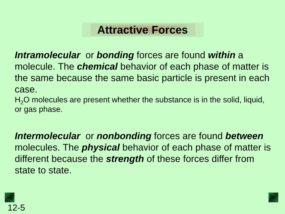
Attractive Forces

Intramolecular or bonding forces are found within a

molecule. The chemical behavior of each phase of matter is

the same because the same basic particle is present in each

case. H2O molecules are present whether the substance is in the solid, liquid,

or gas phase.

Intermolecular or nonbonding forces are found between

molecules. The physical behavior of each phase of matter is

different because the strength of these forces differ from

state to state.

12-6

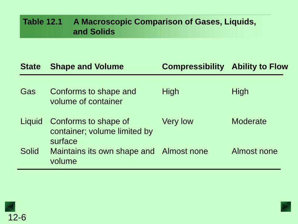
State Shape and Volume Compressibility Ability to Flow

Gas Conforms to shape and

volume of container

High High

Liquid Conforms to shape of

container; volume limited by

surface

Very low Moderate

Solid Maintains its own shape and

volume

Almost none Almost none

Table 12.1 A Macroscopic Comparison of Gases, Liquids,

and Solids

12-7

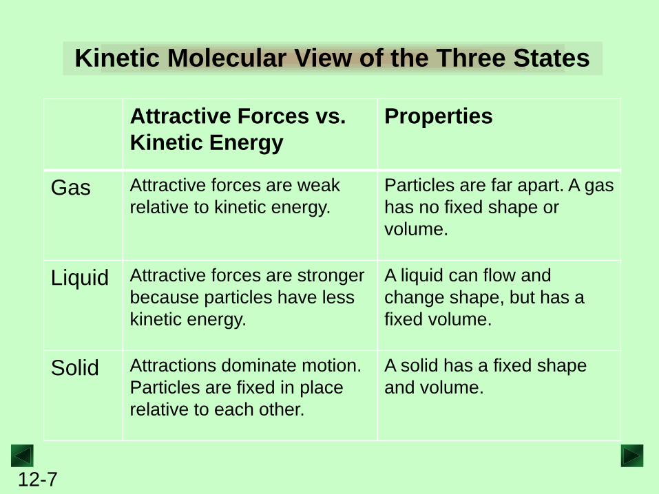
Attractive Forces vs.

Kinetic Energy

Properties

Gas Attractive forces are weak

relative to kinetic energy.

Particles are far apart. A gas

has no fixed shape or

volume.

Liquid Attractive forces are stronger

because particles have less

kinetic energy.

A liquid can flow and

change shape, but has a

fixed volume.

Solid Attractions dominate motion.

Particles are fixed in place

relative to each other.

A solid has a fixed shape

and volume.

Kinetic Molecular View of the Three States

12-8

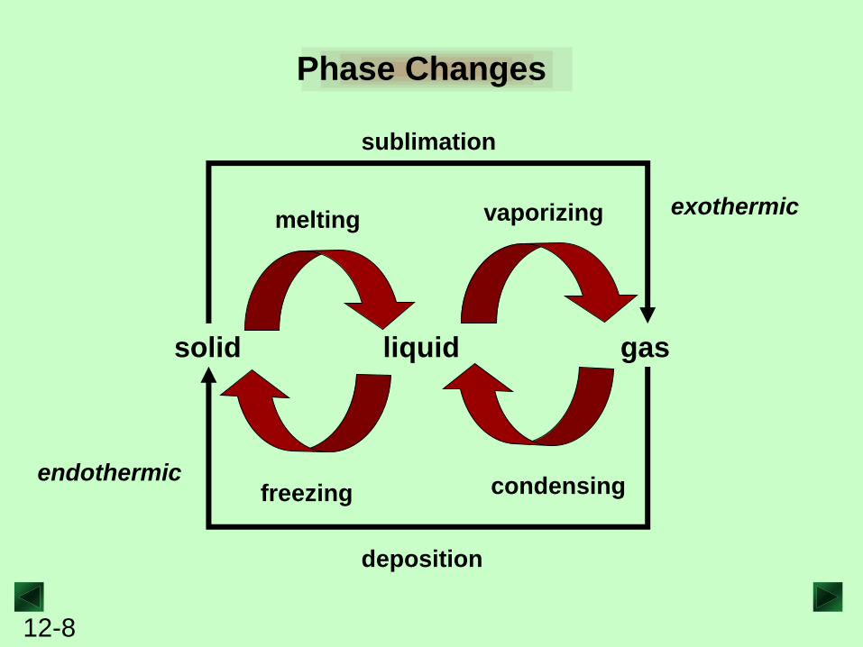
Phase Changes

solid liquid gas

melting

freezing

vaporizing

condensing endothermic

exothermic

deposition

sublimation

12-9

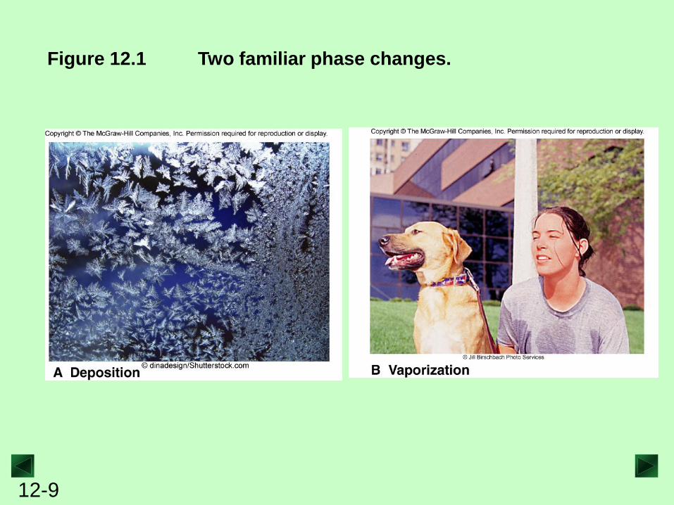
Figure 12.1 Two familiar phase changes.

12-10

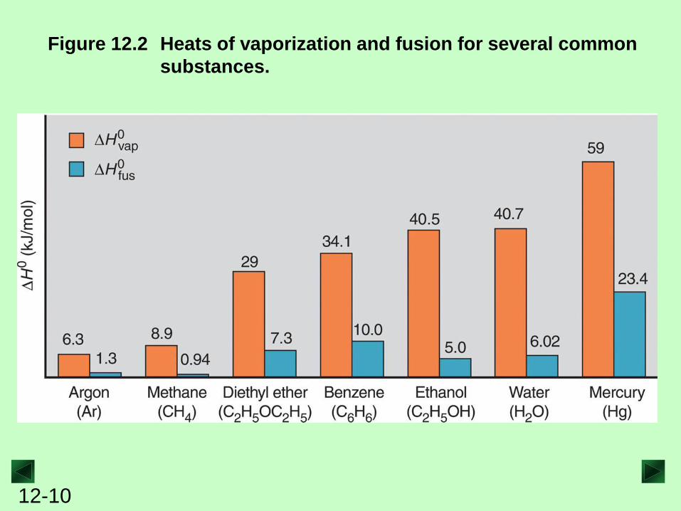
Figure 12.2 Heats of vaporization and fusion for several common

substances.

12-11

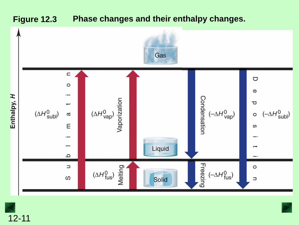
Figure 12.3 Phase changes and their enthalpy changes.

12-12

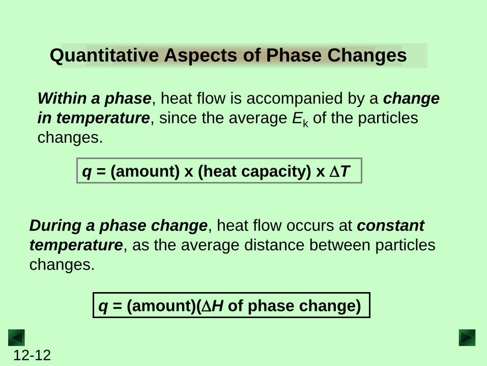
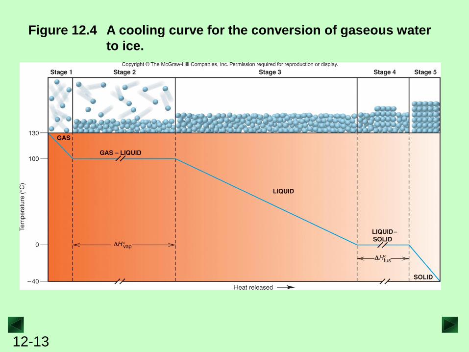
Within a phase, heat flow is accompanied by a change

in temperature, since the average Ek of the particles

changes.

Quantitative Aspects of Phase Changes

q = (amount) x (heat capacity) x DT

q = (amount)(DH of phase change)

During a phase change, heat flow occurs at constant

temperature, as the average distance between particles

changes.

12-13

Figure 12.4 A cooling curve for the conversion of gaseous water

to ice.

12-14

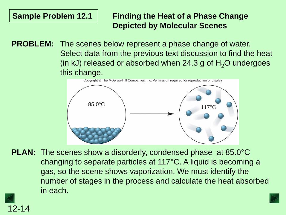
Sample Problem 12.1 Finding the Heat of a Phase Change

Depicted by Molecular Scenes

PROBLEM: The scenes below represent a phase change of water.

Select data from the previous text discussion to find the heat

(in kJ) released or absorbed when 24.3 g of H2O undergoes

this change.

PLAN: The scenes show a disorderly, condensed phase at 85.0°C

changing to separate particles at 117°C. A liquid is becoming a

gas, so the scene shows vaporization. We must identify the

number of stages in the process and calculate the heat absorbed

in each.

12-15

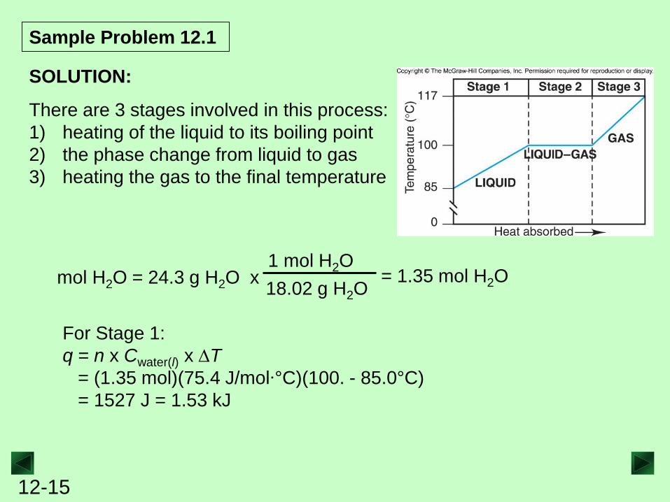
Sample Problem 12.1

SOLUTION:

There are 3 stages involved in this process:

1) heating of the liquid to its boiling point

2) the phase change from liquid to gas

3) heating the gas to the final temperature

mol H2O = 24.3 g H2O x 1 mol H2O

18.02 g H2O = 1.35 mol H2O

For Stage 1:

q = n x Cwater(l) x DT

= (1.35 mol)(75.4 J/mol∙°C)(100. - 85.0°C)

= 1527 J = 1.53 kJ

12-16

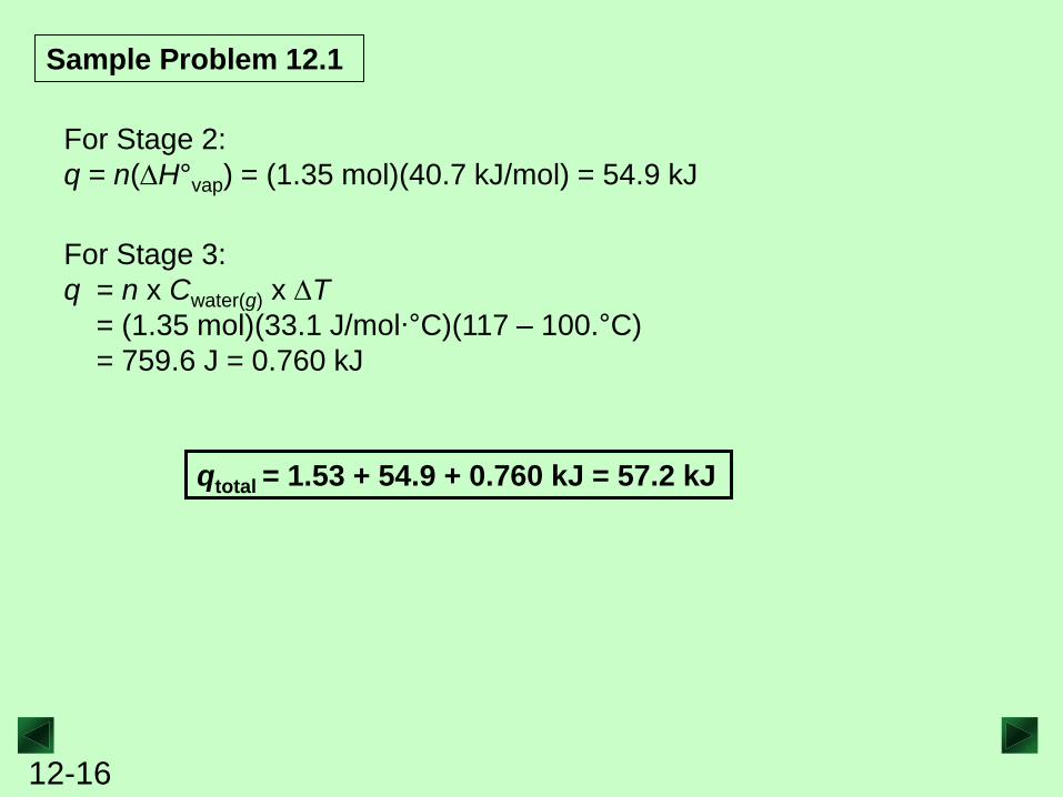
For Stage 2:

q = n(DH°vap) = (1.35 mol)(40.7 kJ/mol) = 54.9 kJ

qtotal = 1.53 + 54.9 + 0.760 kJ = 57.2 kJ

For Stage 3:

q = n x Cwater(g) x DT

= (1.35 mol)(33.1 J/mol∙°C)(117 – 100.°C)

= 759.6 J = 0.760 kJ

Sample Problem 12.1

12-17

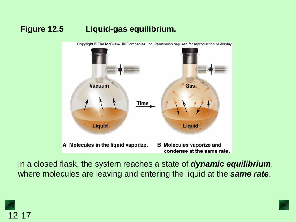
Figure 12.5 Liquid-gas equilibrium.

In a closed flask, the system reaches a state of dynamic equilibrium,

where molecules are leaving and entering the liquid at the same rate.

12-18

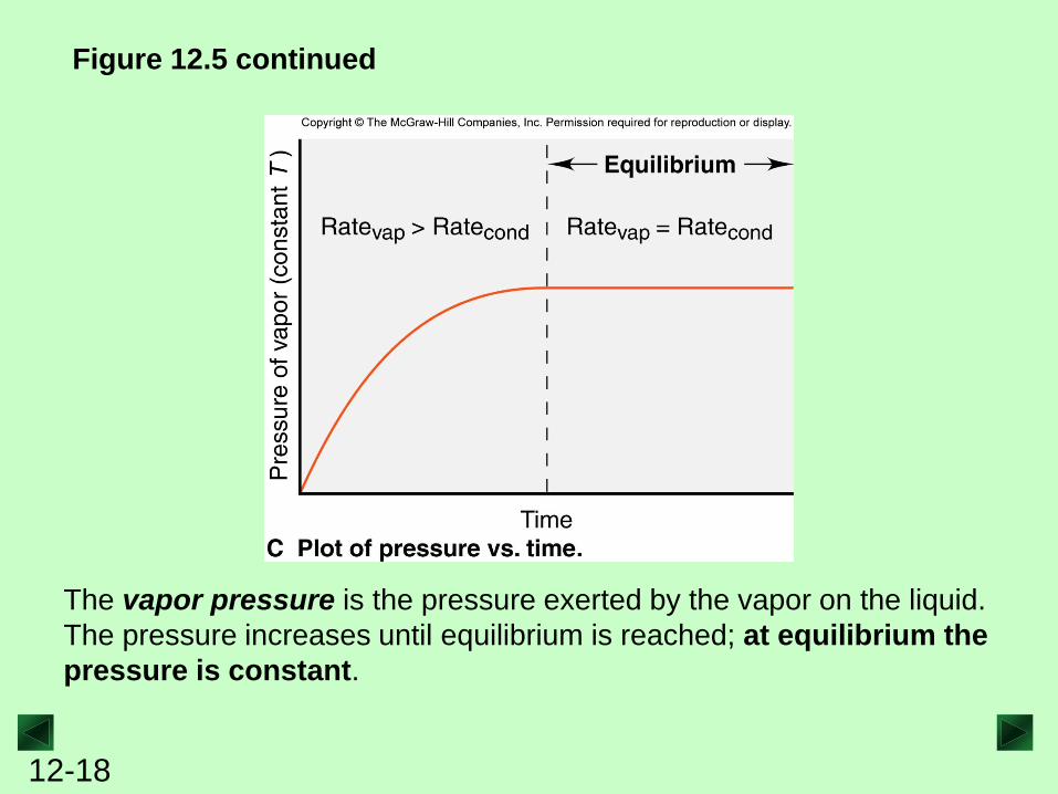
Figure 12.5 continued

The vapor pressure is the pressure exerted by the vapor on the liquid.

The pressure increases until equilibrium is reached; at equilibrium the

pressure is constant.

12-19

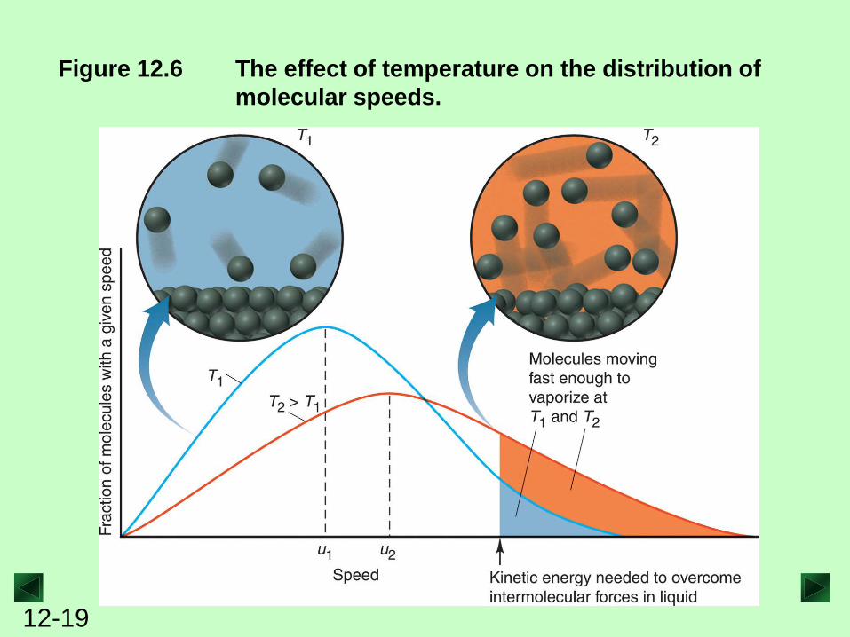
Figure 12.6 The effect of temperature on the distribution of

molecular speeds.

12-20

Factors affecting Vapor Pressure

As temperature increases, the fraction of molecules with

enough energy to enter the vapor phase increases, and the

vapor pressure increases.

The weaker the intermolecular forces, the more easily

particles enter the vapor phase, and the higher the vapor

pressure.

higher T higher P

weaker forces higher P

12-21

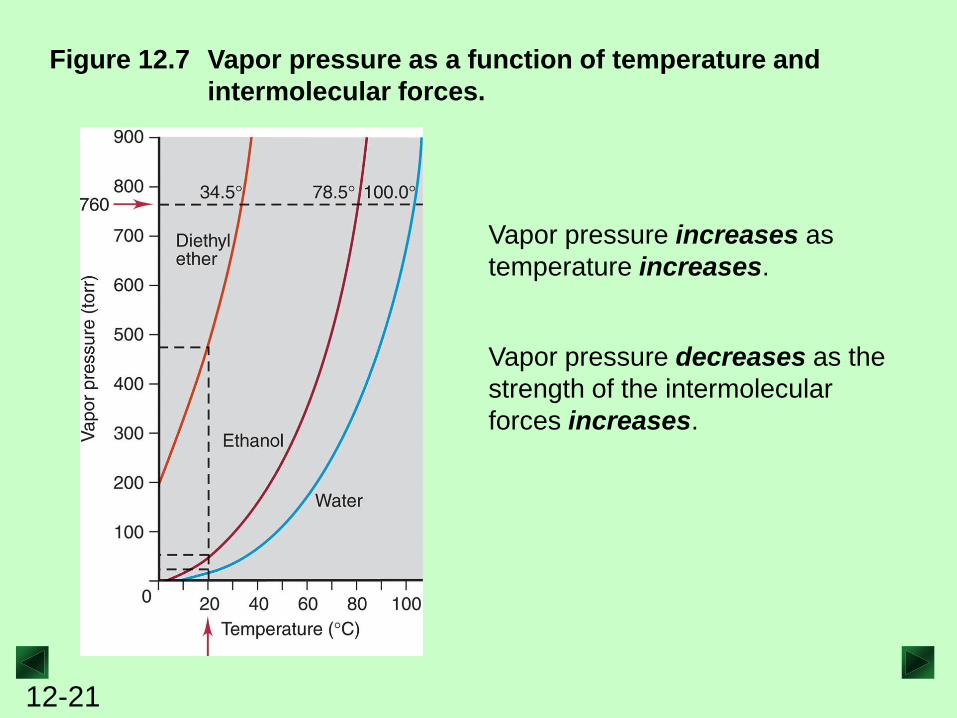
Figure 12.7 Vapor pressure as a function of temperature and

intermolecular forces.

Vapor pressure increases as

temperature increases.

Vapor pressure decreases as the

strength of the intermolecular

forces increases.

12-22

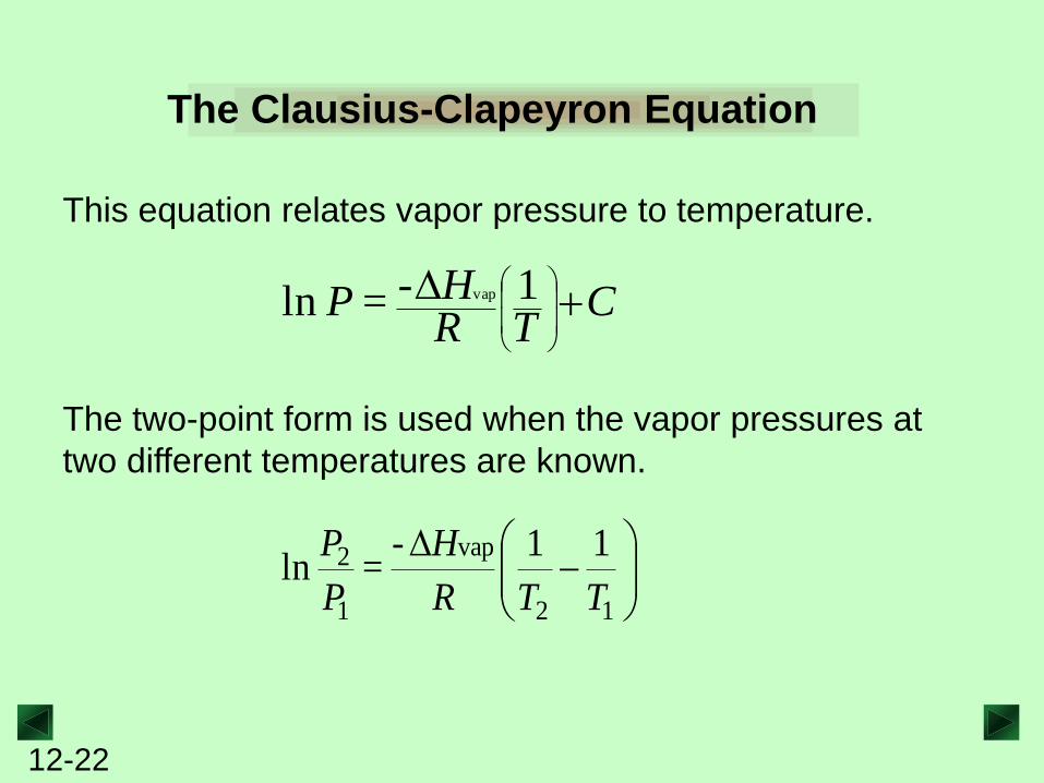
The Clausius-Clapeyron Equation

CTR

HP D

1- = ln vap

This equation relates vapor pressure to temperature.

D

12

vap

1

2 11- = ln

TTR

H

P

P

The two-point form is used when the vapor pressures at

two different temperatures are known.

12-23

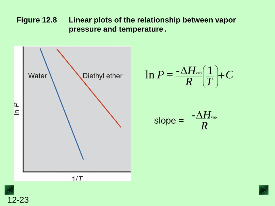
Figure 12.8 Linear plots of the relationship between vapor

pressure and temperature .

CTR

HP D

1- = ln vap

RHvap-D

slope =

12-24

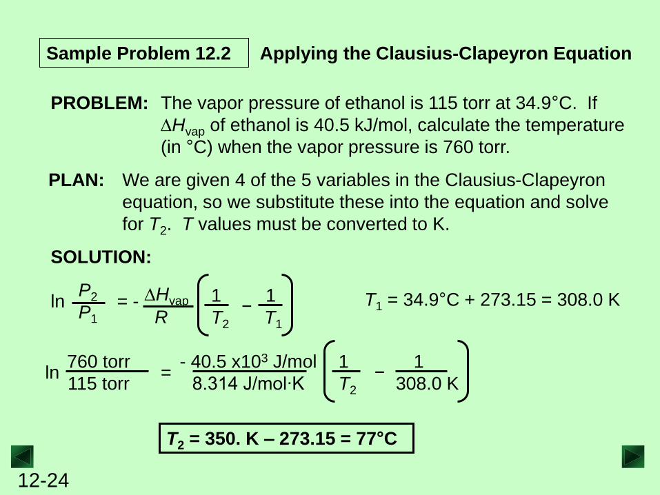
Sample Problem 12.2 Applying the Clausius-Clapeyron Equation

SOLUTION:

PROBLEM: The vapor pressure of ethanol is 115 torr at 34.9°C. If

DHvap of ethanol is 40.5 kJ/mol, calculate the temperature

(in °C) when the vapor pressure is 760 torr.

PLAN: We are given 4 of the 5 variables in the Clausius-Clapeyron

equation, so we substitute these into the equation and solve

for T2. T values must be converted to K.

T1 = 34.9°C + 273.15 = 308.0 K

ln 760 torr

115 torr =

- 40.5 x103 J/mol

8.314 J/mol∙K

1

T2

1

308.0 K −

T2 = 350. K – 273.15 = 77°C

P2

P1

ln = - DHvap

R

1

T2

1

T1

−

12-25

Vapor Pressure and Boiling Point

The boiling point of a liquid is the temperature at which the

vapor pressure equals the external pressure.

As the external pressure on a liquid increases, the boiling

point increases.

The normal boiling point of a substance is observed at

standard atmospheric pressure or 760 torr.

12-26

Figure 12.9 Iodine subliming.

After the solid sublimes, vapor deposits on a cold surface.

12-27

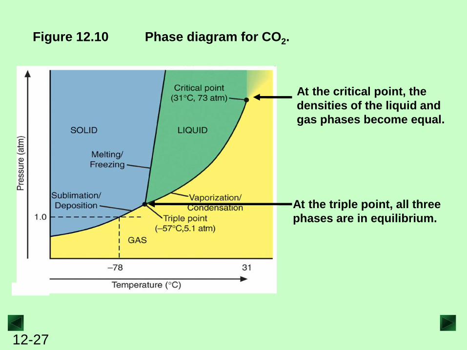
Figure 12.10 Phase diagram for CO2.

At the critical point, the

densities of the liquid and

gas phases become equal.

At the triple point, all three

phases are in equilibrium.

12-28

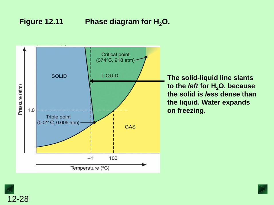
Figure 12.11 Phase diagram for H2O.

The solid-liquid line slants

to the left for H2O, because

the solid is less dense than

the liquid. Water expands

on freezing.

12-29

The Nature of Intermolecular Forces

Intermolecular forces are relatively weak compared to

bonding forces because they involve smaller charges that

are farther apart.

Intermolecular forces arise from the attraction between

molecules with partial charges, or between ions and

molecules.

12-30

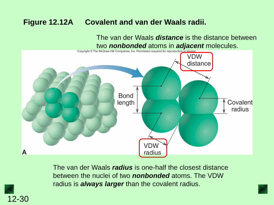
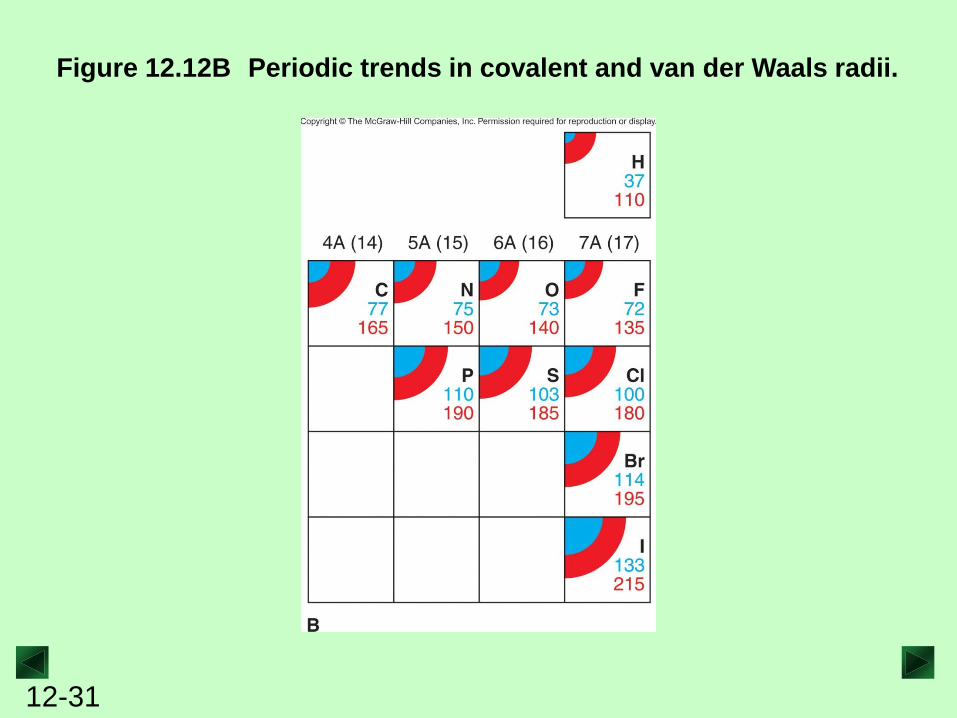
Figure 12.12A Covalent and van der Waals radii.

The van der Waals distance is the distance between

two nonbonded atoms in adjacent molecules.

The van der Waals radius is one-half the closest distance

between the nuclei of two nonbonded atoms. The VDW

radius is always larger than the covalent radius.

12-31

Figure 12.12B Periodic trends in covalent and van der Waals radii.

12-32

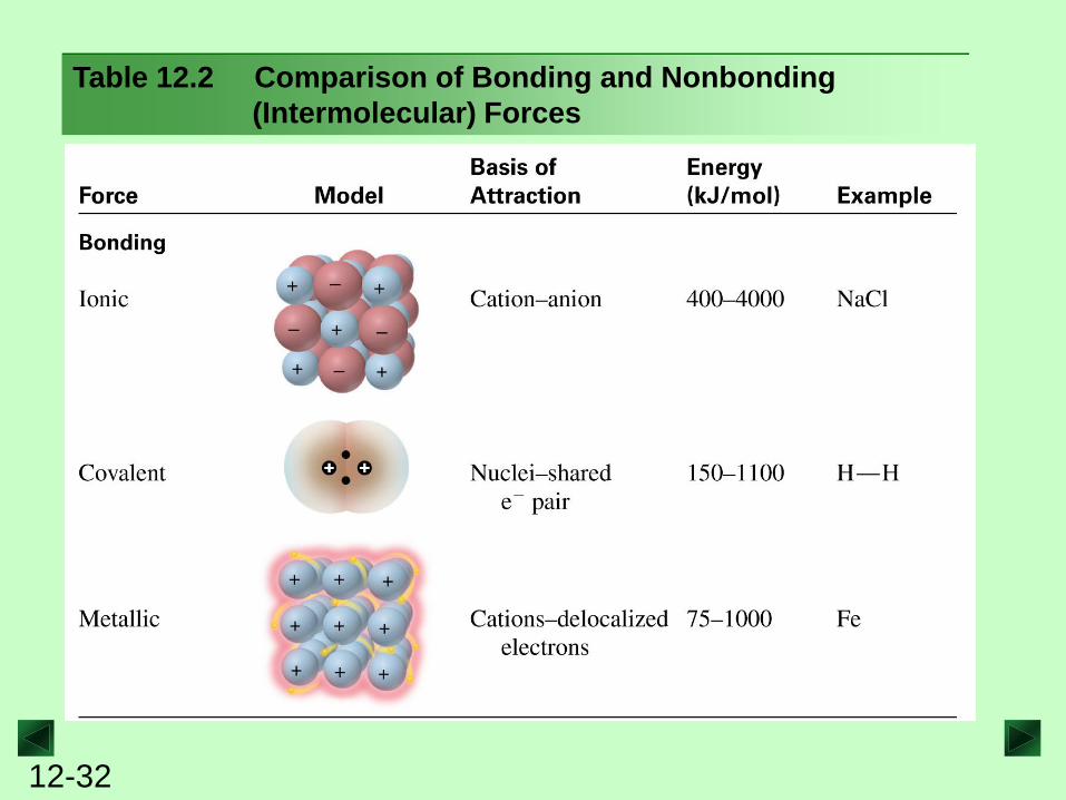
Table 12.2 Comparison of Bonding and Nonbonding

(Intermolecular) Forces

12-33

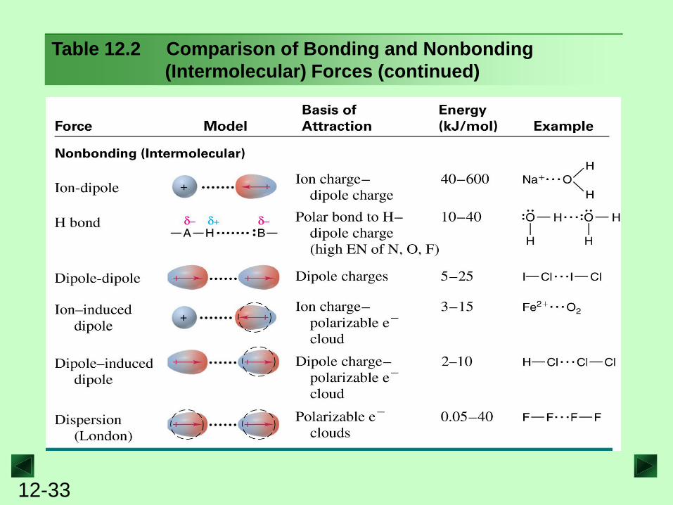
Table 12.2 Comparison of Bonding and Nonbonding

(Intermolecular) Forces (continued)

12-34

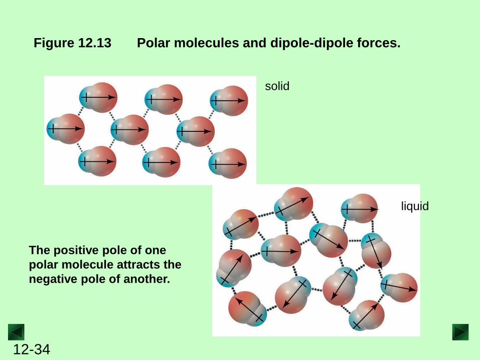
Figure 12.13 Polar molecules and dipole-dipole forces.

solid

liquid

The positive pole of one

polar molecule attracts the

negative pole of another.

12-35

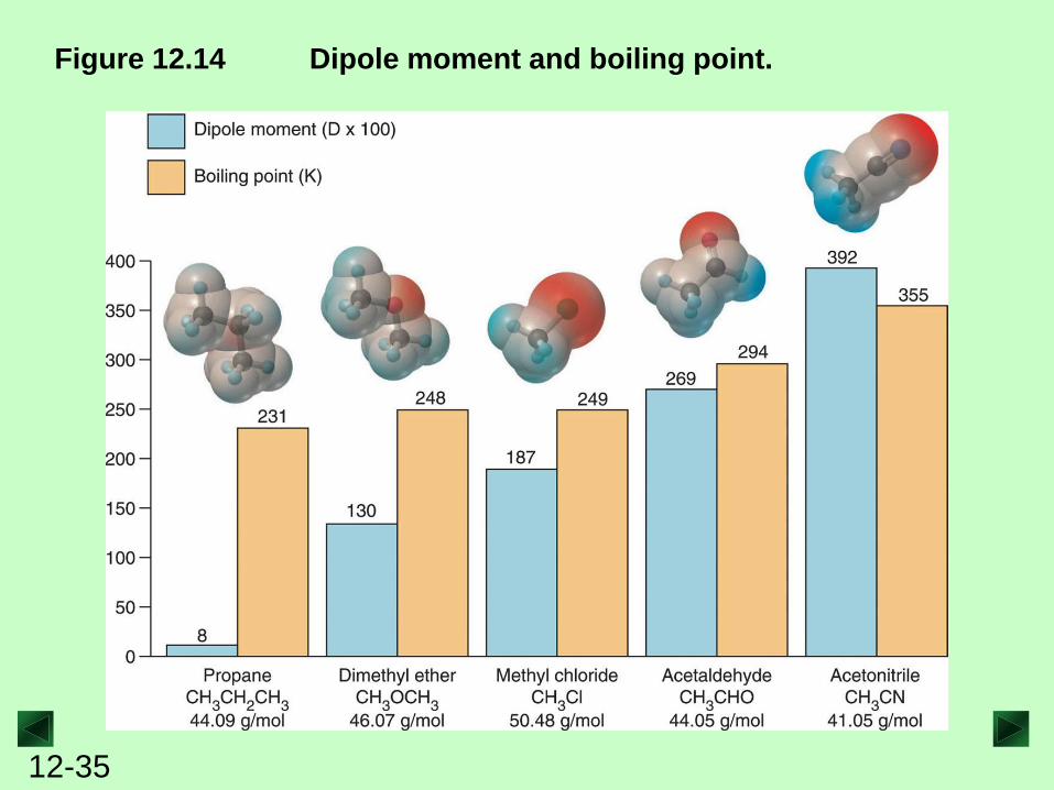
Figure 12.14 Dipole moment and boiling point.

12-36

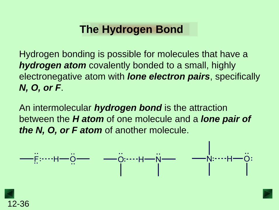
The Hydrogen Bond

Hydrogen bonding is possible for molecules that have a

hydrogen atom covalently bonded to a small, highly

electronegative atom with lone electron pairs, specifically

N, O, or F.

An intermolecular hydrogen bond is the attraction

between the H atom of one molecule and a lone pair of

the N, O, or F atom of another molecule.

12-37

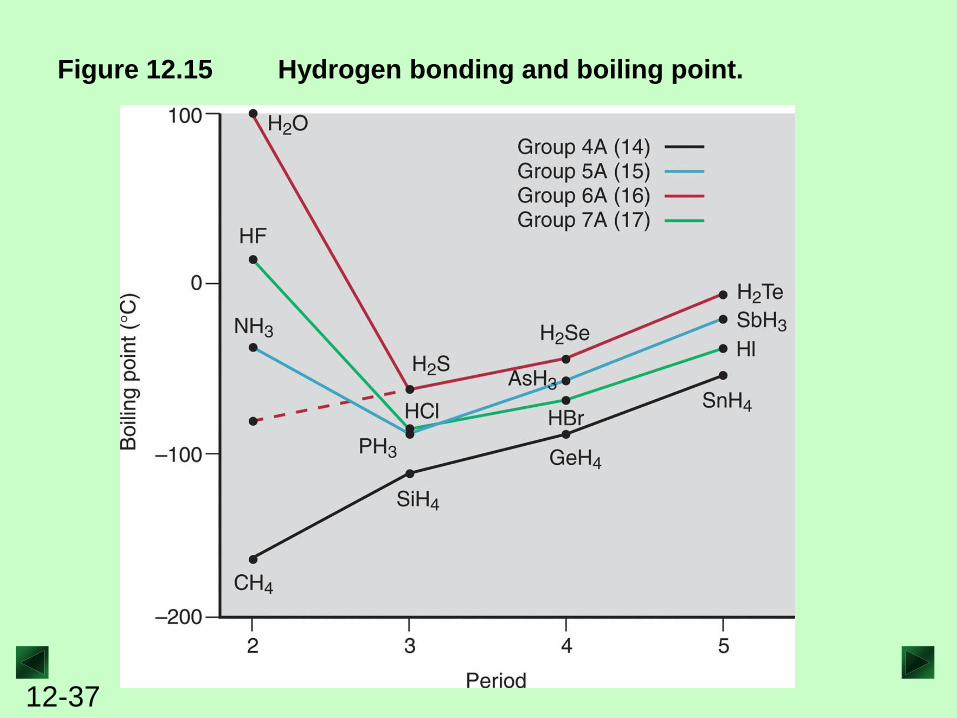
Figure 12.15 Hydrogen bonding and boiling point.

12-38

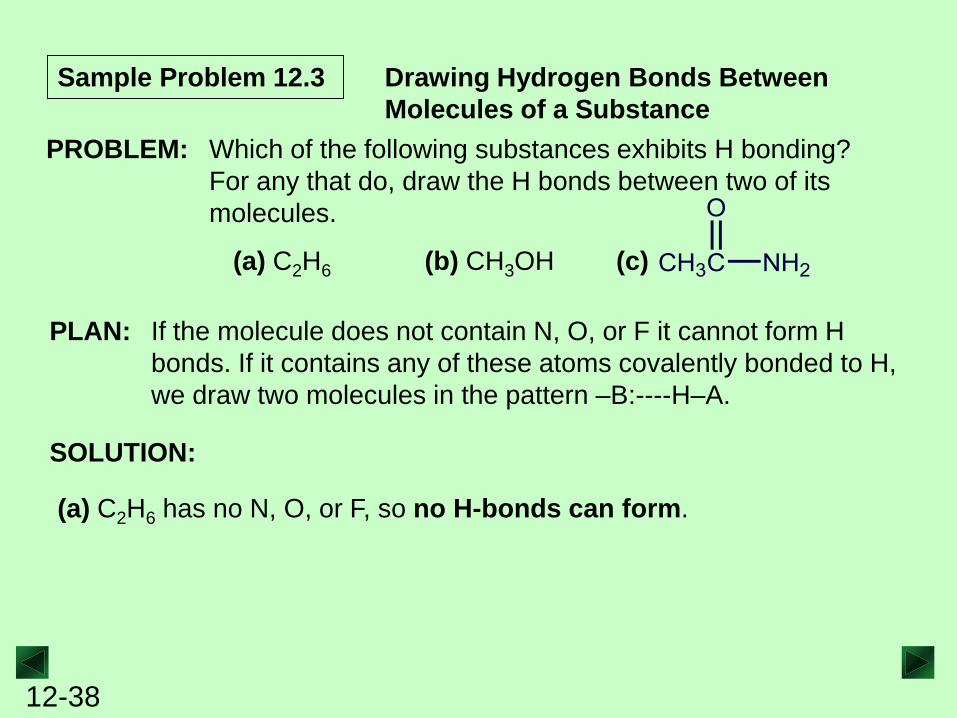
Sample Problem 12.3 Drawing Hydrogen Bonds Between

Molecules of a Substance

SOLUTION:

PLAN: If the molecule does not contain N, O, or F it cannot form H

bonds. If it contains any of these atoms covalently bonded to H,

we draw two molecules in the pattern –B:----H–A.

(a) C2H6 has no N, O, or F, so no H-bonds can form.

PROBLEM: Which of the following substances exhibits H bonding?

For any that do, draw the H bonds between two of its

molecules.

(a) C2H6 (b) CH3OH (c)

12-39

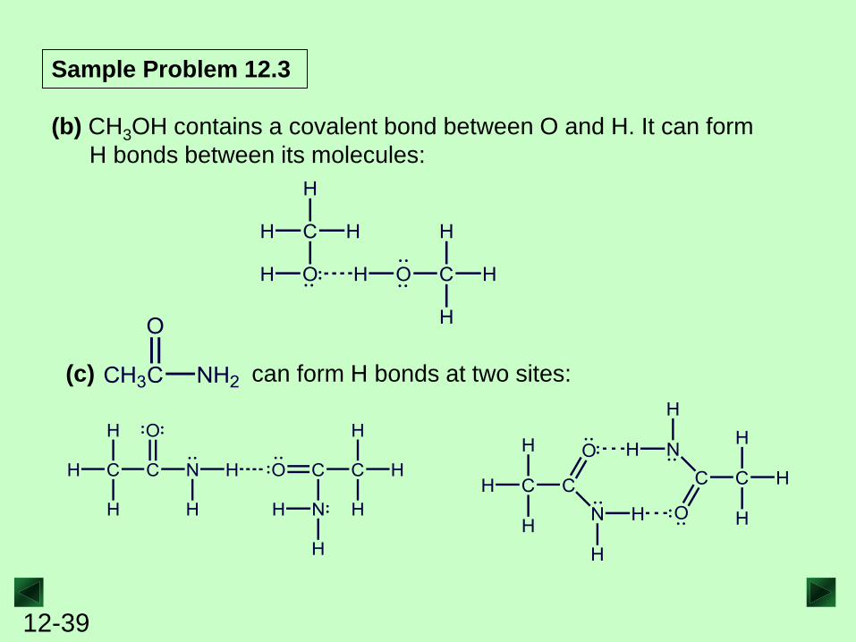
Sample Problem 12.3

(b) CH3OH contains a covalent bond between O and H. It can form

H bonds between its molecules:

(c) can form H bonds at two sites:

12-40

Polarizability and Induced Dipoles

A nearby electric field can induce a distortion in the

electron cloud of an atom, ion, or molecule.

- For a nonpolar molecule, this induces a temporary

dipole moment.

- For a polar molecule, the field enhances the existing

dipole moment.

The polarizability of a particle is the ease with which its

electron cloud is distorted.

12-41

Trends in Polarizability

Smaller particles are less polarizable than larger ones

because their electrons are held more tightly.

Polarizability increases down a group because atomic size

increases and larger electron clouds distort more easily.

Polarizability decreases across a period because of

increasing Zeff.

Cations are smaller than their parent atoms and less

polarizable; anions show the opposite trend.

12-42

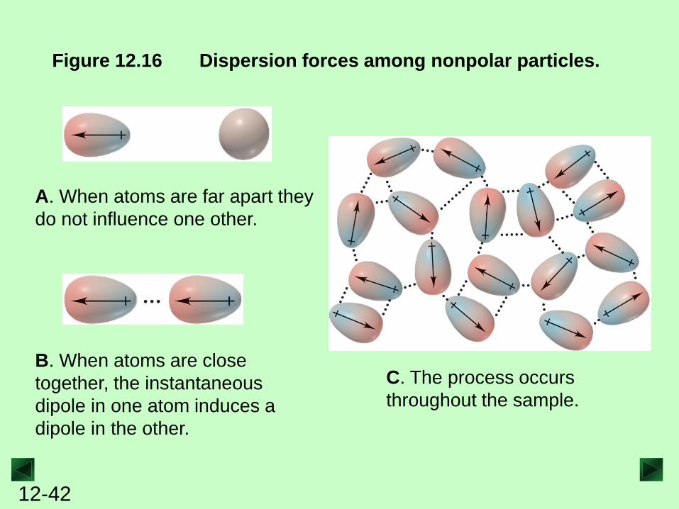
Figure 12.16 Dispersion forces among nonpolar particles.

A. When atoms are far apart they

do not influence one other.

B. When atoms are close

together, the instantaneous

dipole in one atom induces a

dipole in the other.

C. The process occurs

throughout the sample.

12-43

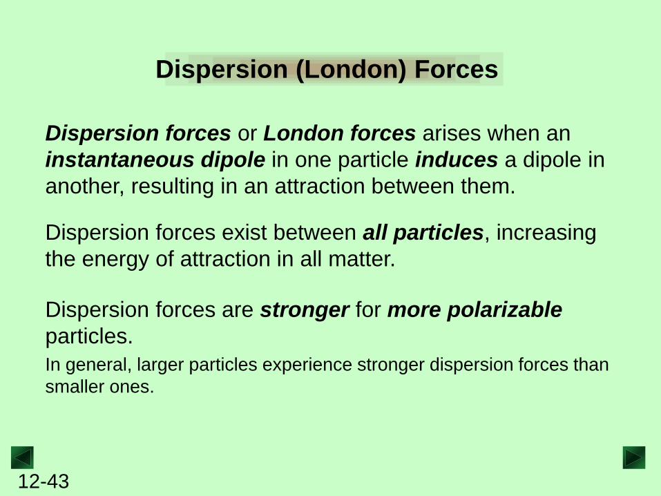
Dispersion (London) Forces

Dispersion forces or London forces arises when an

instantaneous dipole in one particle induces a dipole in

another, resulting in an attraction between them.

Dispersion forces exist between all particles, increasing

the energy of attraction in all matter.

Dispersion forces are stronger for more polarizable

particles.

In general, larger particles experience stronger dispersion forces than

smaller ones.

12-44

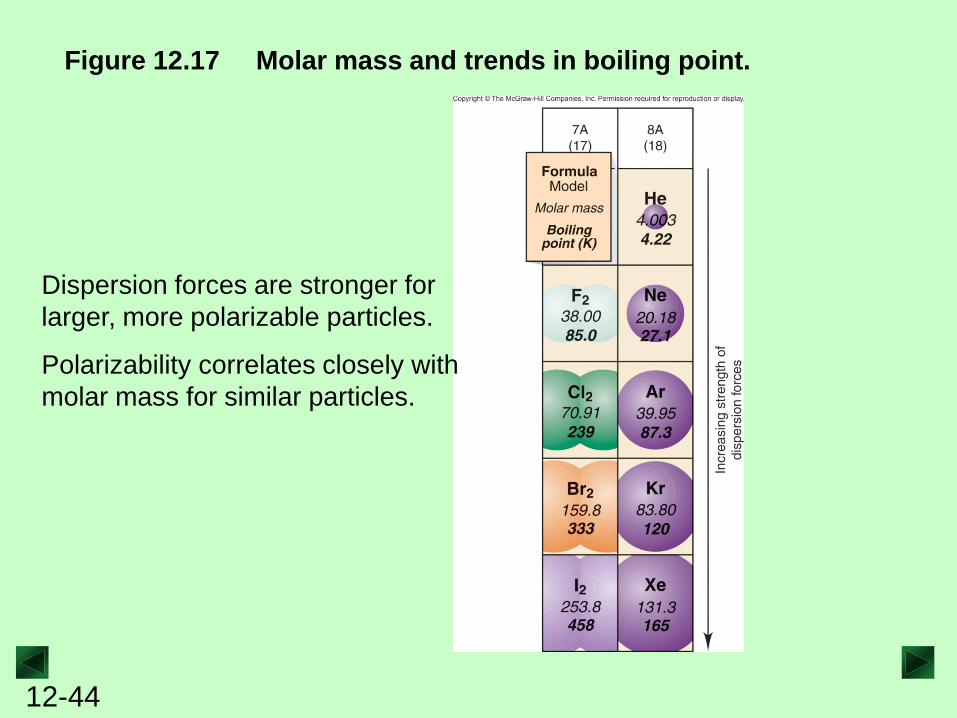
Figure 12.17 Molar mass and trends in boiling point.

Dispersion forces are stronger for

larger, more polarizable particles.

Polarizability correlates closely with

molar mass for similar particles.

12-45

Figure 12.18 Molecular shape, intermolecular contact, and

boiling point.

There are more points

at which dispersion

forces act.

There are fewer points

at which dispersion

forces act.

12-46

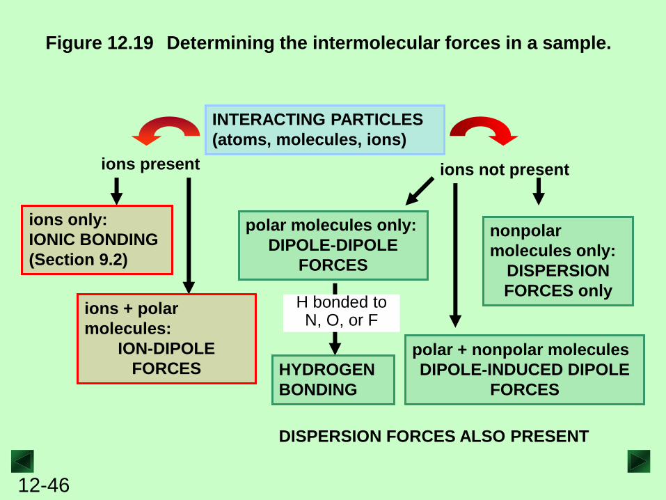
Figure 12.19 Determining the intermolecular forces in a sample.

ions not present ions present

DISPERSION FORCES ALSO PRESENT

ions only:

IONIC BONDING

(Section 9.2)

ions + polar

molecules:

ION-DIPOLE

FORCES

INTERACTING PARTICLES

(atoms, molecules, ions)

polar molecules only:

DIPOLE-DIPOLE

FORCES

H bonded to N, O, or F

HYDROGEN

BONDING

polar + nonpolar molecules

DIPOLE-INDUCED DIPOLE

FORCES

nonpolar

molecules only:

DISPERSION

FORCES only

12-47

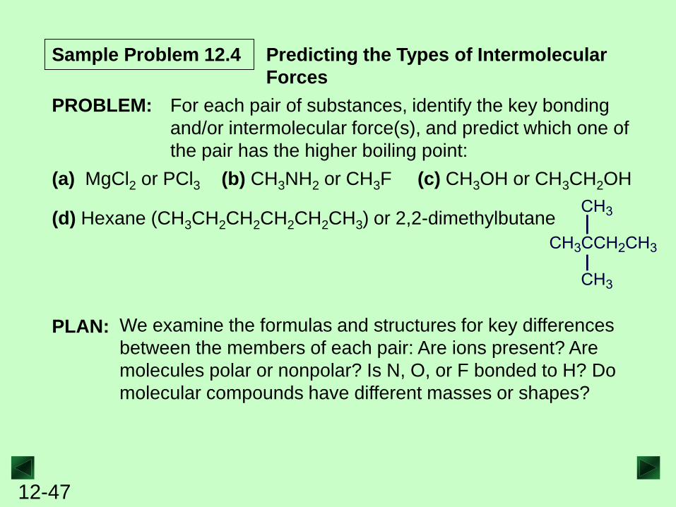
Sample Problem 12.4 Predicting the Types of Intermolecular

Forces

PLAN: We examine the formulas and structures for key differences

between the members of each pair: Are ions present? Are

molecules polar or nonpolar? Is N, O, or F bonded to H? Do

molecular compounds have different masses or shapes?

PROBLEM: For each pair of substances, identify the key bonding

and/or intermolecular force(s), and predict which one of

the pair has the higher boiling point:

(a) MgCl2 or PCl3 (b) CH3NH2 or CH3F (c) CH3OH or CH3CH2OH

(d) Hexane (CH3CH2CH2CH2CH2CH3) or 2,2-dimethylbutane

12-48

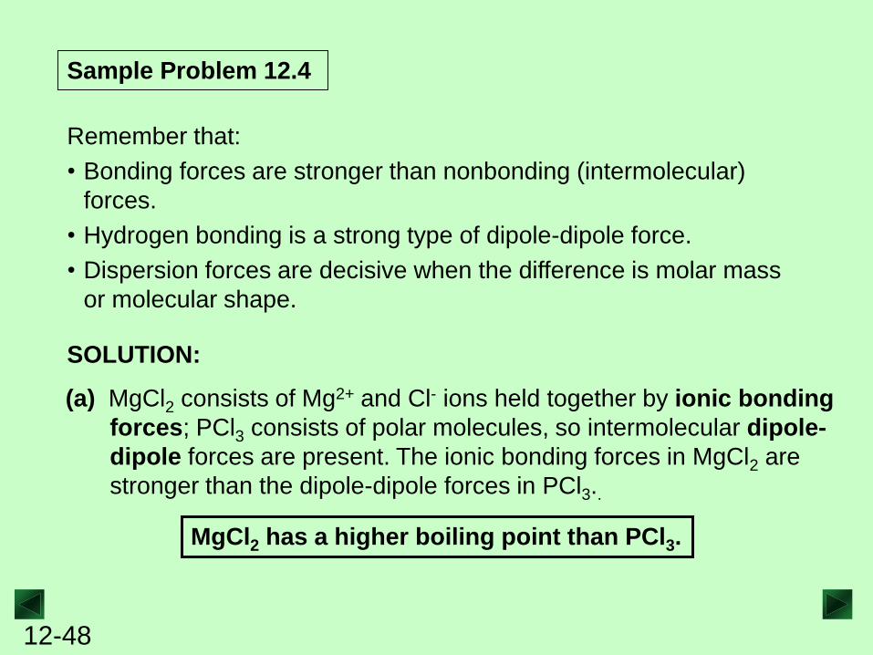
Remember that:

• Bonding forces are stronger than nonbonding (intermolecular)

forces.

• Hydrogen bonding is a strong type of dipole-dipole force.

• Dispersion forces are decisive when the difference is molar mass

or molecular shape.

Sample Problem 12.4

SOLUTION:

(a) MgCl2 consists of Mg2+ and Cl- ions held together by ionic bonding

forces; PCl3 consists of polar molecules, so intermolecular dipole-

dipole forces are present. The ionic bonding forces in MgCl2 are

stronger than the dipole-dipole forces in PCl3..

MgCl2 has a higher boiling point than PCl3.

12-49

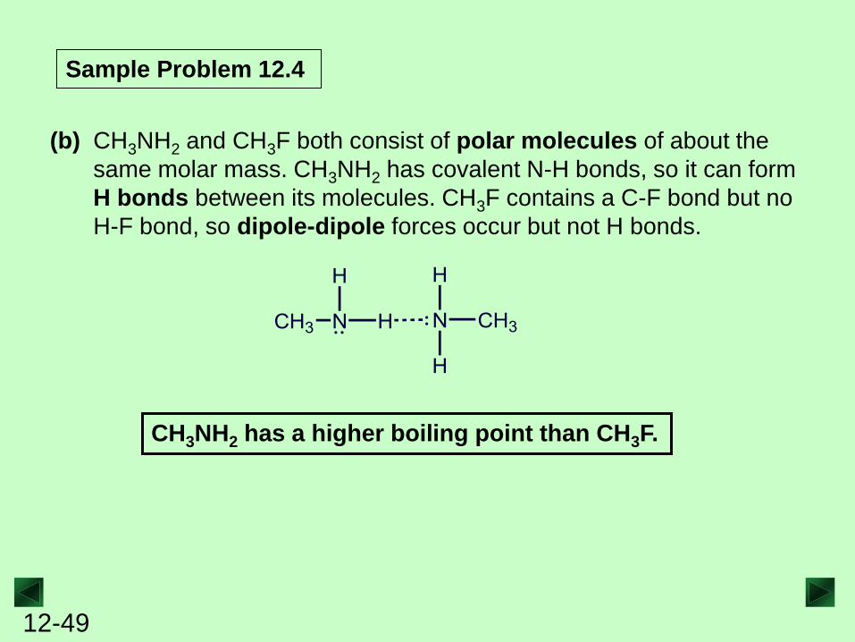
Sample Problem 12.4

(b) CH3NH2 and CH3F both consist of polar molecules of about the

same molar mass. CH3NH2 has covalent N-H bonds, so it can form

H bonds between its molecules. CH3F contains a C-F bond but no

H-F bond, so dipole-dipole forces occur but not H bonds.

CH3NH2 has a higher boiling point than CH3F.

12-50

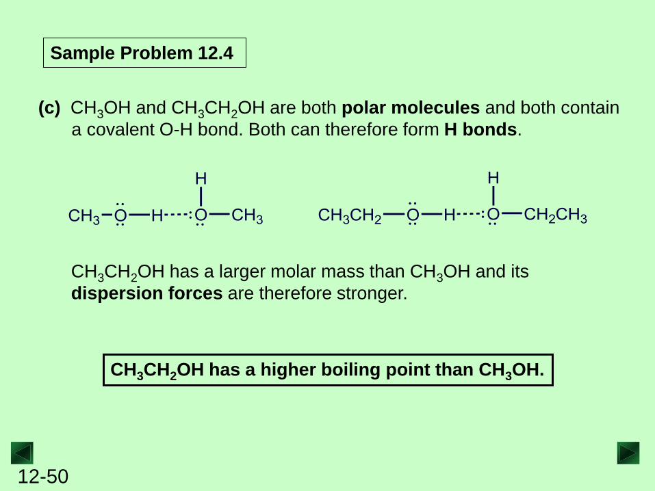
Sample Problem 12.4

(c) CH3OH and CH3CH2OH are both polar molecules and both contain

a covalent O-H bond. Both can therefore form H bonds.

CH3CH2OH has a higher boiling point than CH3OH.

CH3CH2OH has a larger molar mass than CH3OH and its

dispersion forces are therefore stronger.

12-51

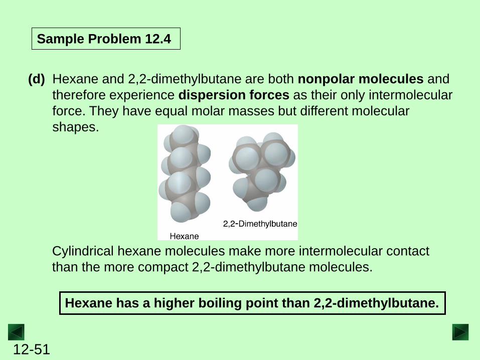
(d) Hexane and 2,2-dimethylbutane are both nonpolar molecules and

therefore experience dispersion forces as their only intermolecular

force. They have equal molar masses but different molecular

shapes.

Sample Problem 12.4

Cylindrical hexane molecules make more intermolecular contact

than the more compact 2,2-dimethylbutane molecules.

Hexane has a higher boiling point than 2,2-dimethylbutane.

12-52

Sample Problem 12.4

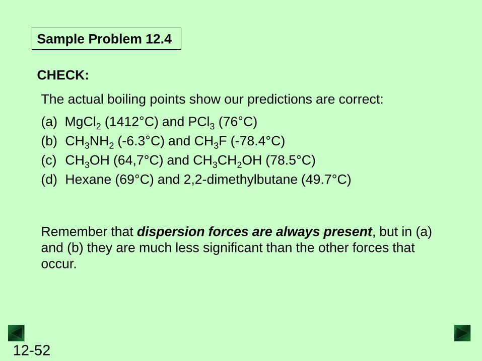
CHECK:

The actual boiling points show our predictions are correct:

(a) MgCl2 (1412°C) and PCl3 (76°C)

(b) CH3NH2 (-6.3°C) and CH3F (-78.4°C)

(c) CH3OH (64,7°C) and CH3CH2OH (78.5°C)

(d) Hexane (69°C) and 2,2-dimethylbutane (49.7°C)

Remember that dispersion forces are always present, but in (a)

and (b) they are much less significant than the other forces that

occur.

12-53

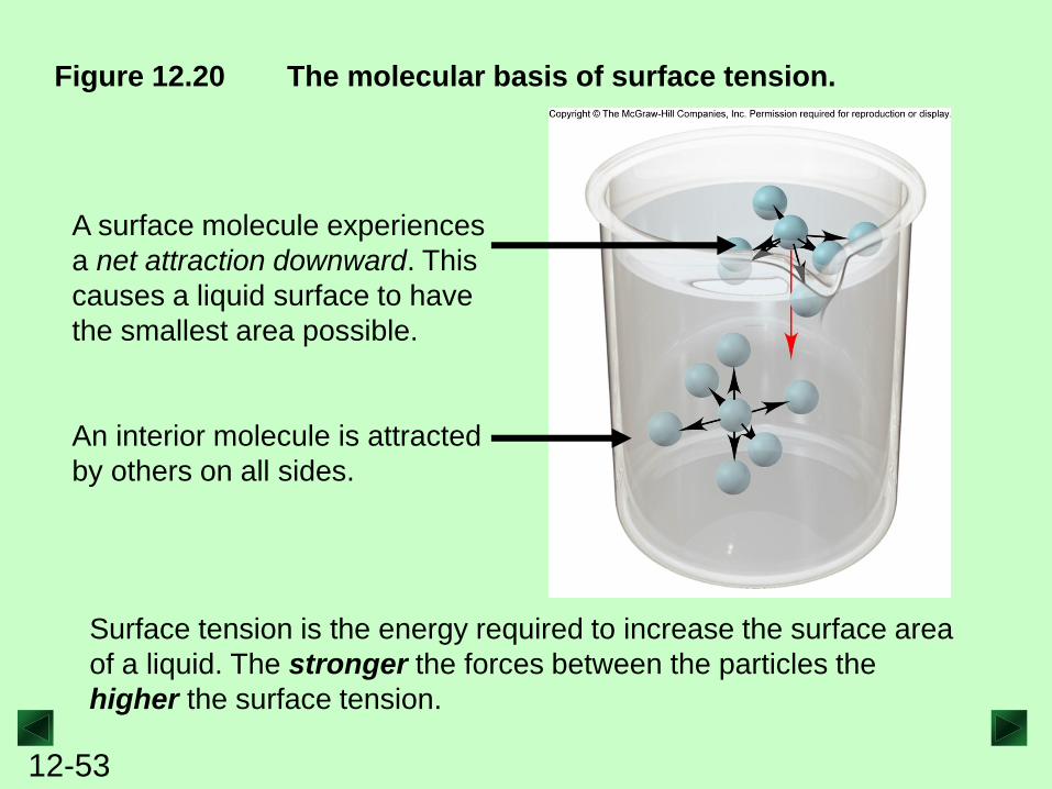
Figure 12.20 The molecular basis of surface tension.

An interior molecule is attracted

by others on all sides.

A surface molecule experiences

a net attraction downward. This

causes a liquid surface to have

the smallest area possible.

Surface tension is the energy required to increase the surface area

of a liquid. The stronger the forces between the particles the

higher the surface tension.

12-54

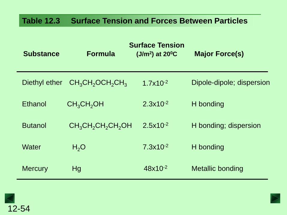
Substance Formula

Surface Tension

(J/m2) at 200C Major Force(s)

Diethyl ether

Ethanol

Butanol

Water

Mercury

Dipole-dipole; dispersion

H bonding

H bonding; dispersion

H bonding

Metallic bonding

1.7x10-2

2.3x10-2

2.5x10-2

7.3x10-2

48x10-2

CH3CH2OCH2CH3

CH3CH2OH

CH3CH2CH2CH2OH

H2O

Hg

Table 12.3 Surface Tension and Forces Between Particles

12-55

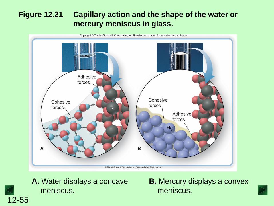
Figure 12.21 Capillary action and the shape of the water or

mercury meniscus in glass.

A. Water displays a concave

meniscus.

B. Mercury displays a convex

meniscus.

12-56

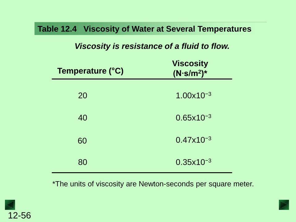
Table 12.4 Viscosity of Water at Several Temperatures

Temperature (°C) Viscosity

(N∙s/m2)*

20

40

60

80

1.00x10−3

0.65x10−3

0.47x10−3

0.35x10−3

*The units of viscosity are Newton-seconds per square meter.

Viscosity is resistance of a fluid to flow.

12-57

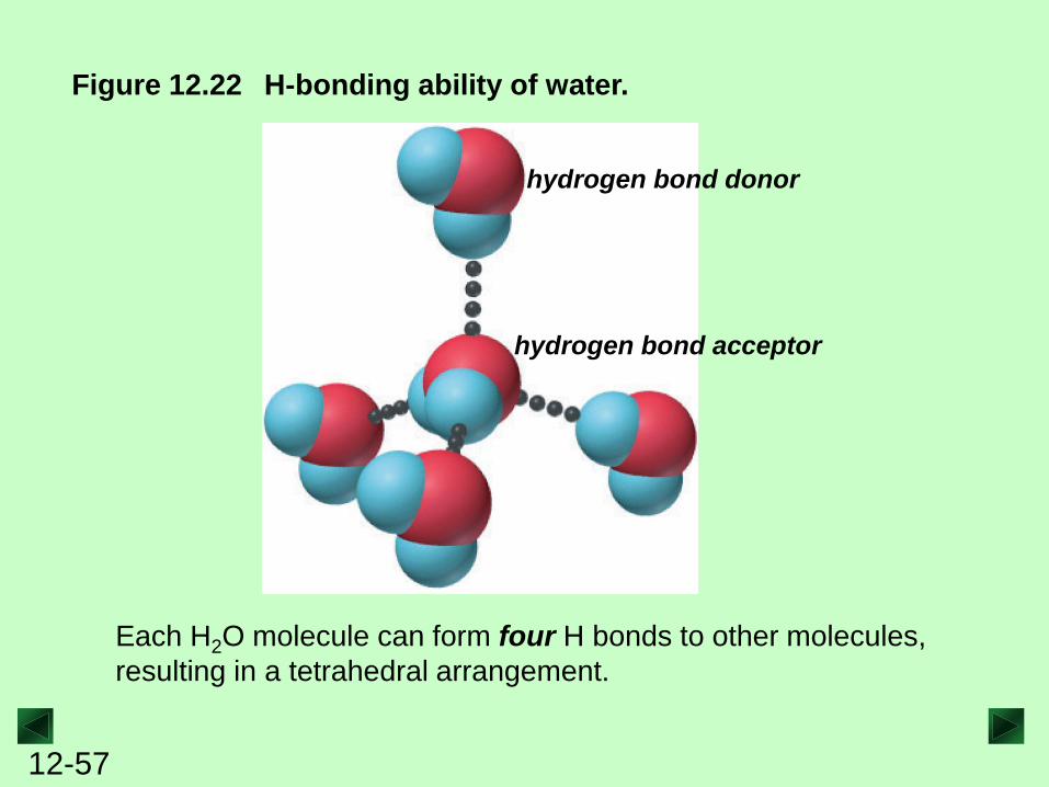
Figure 12.22 H-bonding ability of water.

hydrogen bond donor

hydrogen bond acceptor

Each H2O molecule can form four H bonds to other molecules,

resulting in a tetrahedral arrangement.

12-58

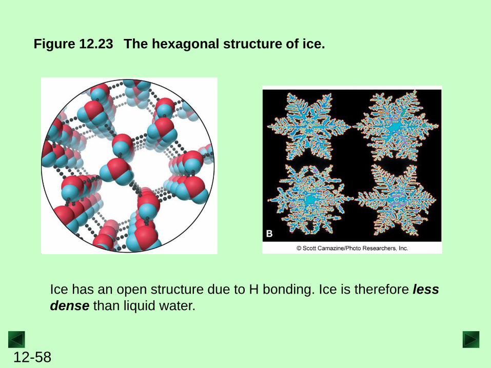
Figure 12.23 The hexagonal structure of ice.

Ice has an open structure due to H bonding. Ice is therefore less

dense than liquid water.

12-59

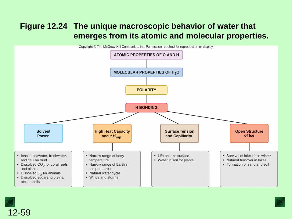
Figure 12.24 The unique macroscopic behavior of water that

emerges from its atomic and molecular properties.

12-60

The Solid State

Solids are divided into two categories:

Crystalline solids have well defined shapes due to the

orderly arrangement of their particles.

Amorphous solids lack orderly arrangement and have

poorly defined shapes.

A crystal is composed of particles packed in an orderly

three-dimensional array called the crystal lattice.

12-61

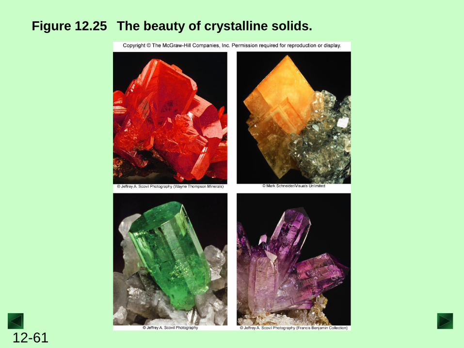
Figure 12.25 The beauty of crystalline solids.

12-62

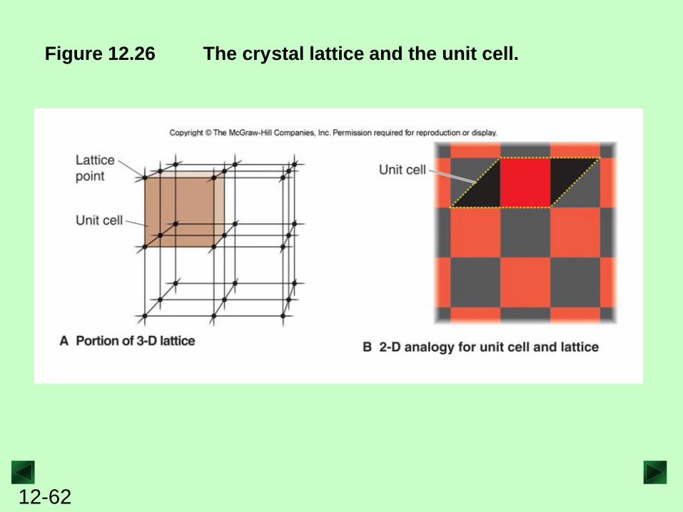
Figure 12.26 The cry stal lattice and the unit cell.

12-63

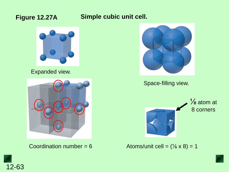
Figure 12.27A Simple cubic unit cell.

Atoms/unit cell = (⅛ x 8) = 1

⅛ atom at

8 corners

Coordination number = 6

Expanded view.

Space-filling view.

12-64

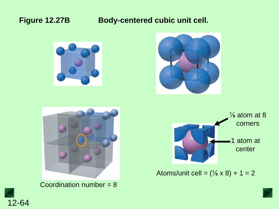
Figure 12.27B Body-centered cubic unit cell.

⅛ atom at 8

corners

1 atom at

center

Atoms/unit cell = (⅛ x 8) + 1 = 2

Coordination number = 8

12-65

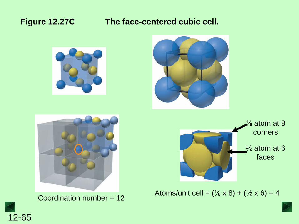
Figure 12.27C The face-centered cubic cell.

Atoms/unit cell = (⅛ x 8) + (½ x 6) = 4

⅛ atom at 8

corners

½ atom at 6

faces

Coordination number = 12

12-66

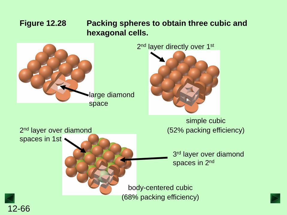
Figure 12.28 Packing spheres to obtain three cubic and

hexagonal cells.

simple cubic

(52% packing efficiency)

body-centered cubic

(68% packing efficiency)

large diamond

space

2nd layer directly over 1st

2nd layer over diamond

spaces in 1st

3rd layer over diamond

spaces in 2nd

12-67

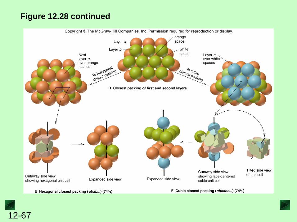
Figure 12.28 continued

12-68

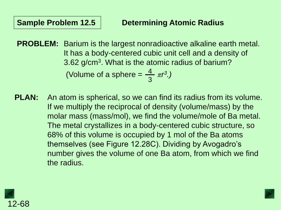
Sample Problem 12.5 Determining Atomic Radius

PLAN: An atom is spherical, so we can find its radius from its volume.

If we multiply the reciprocal of density (volume/mass) by the

molar mass (mass/mol), we find the volume/mole of Ba metal.

The metal crystallizes in a body-centered cubic structure, so

68% of this volume is occupied by 1 mol of the Ba atoms

themselves (see Figure 12.28C). Dividing by Avogadro’s

number gives the volume of one Ba atom, from which we find

the radius.

PROBLEM: Barium is the largest nonradioactive alkaline earth metal.

It has a body-centered cubic unit cell and a density of

3.62 g/cm3. What is the atomic radius of barium?

(Volume of a sphere = πr3.) 4

3

12-69

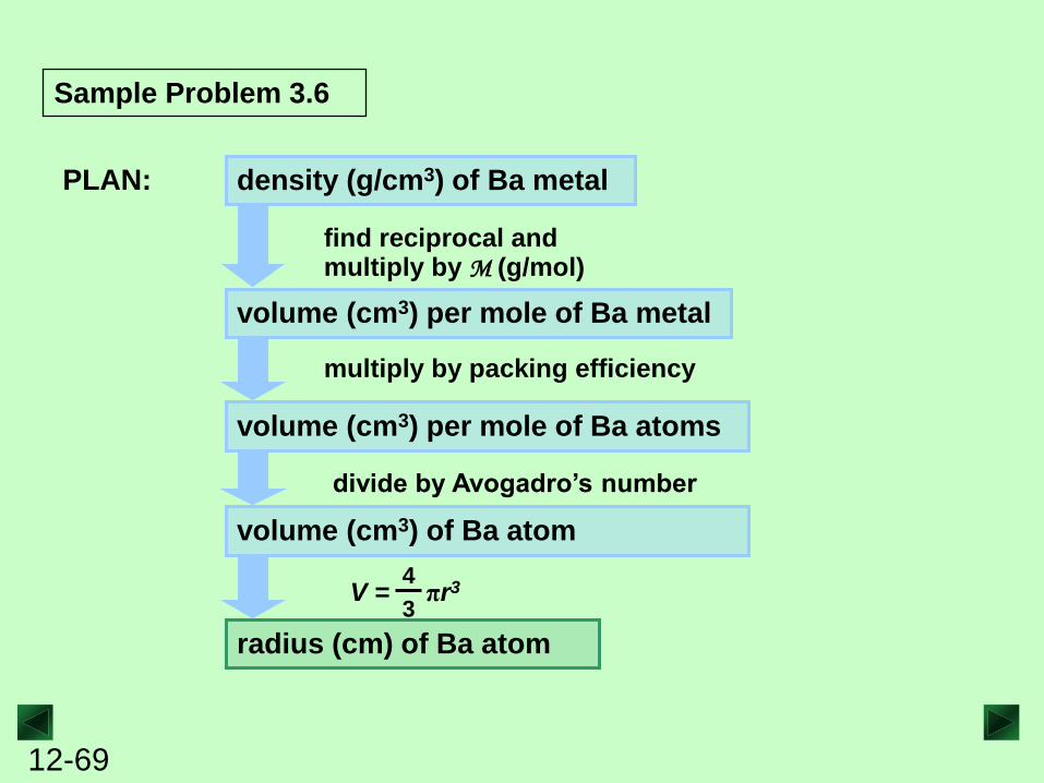
Sample Problem 3.6

PLAN:

find reciprocal and multiply by M (g/mol)

multiply by packing efficiency

divide by Avogadro’s number

radius (cm) of Ba atom

density (g/cm3) of Ba metal

volume (cm3) per mole of Ba metal

volume (cm3) per mole of Ba atoms

volume (cm3) of Ba atom

V = πr3 4

3

12-70

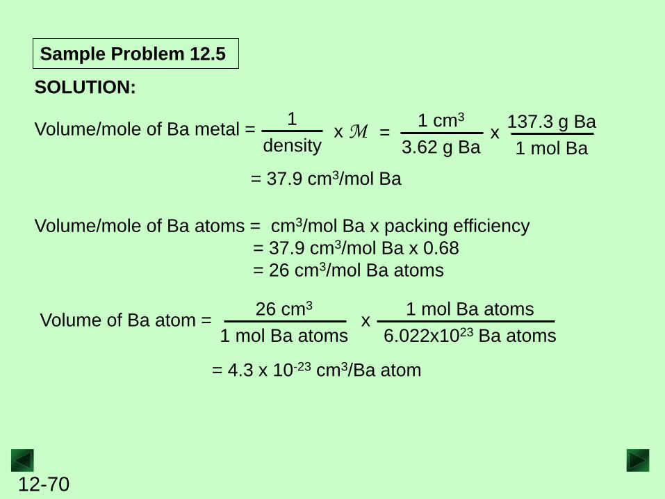
Sample Problem 12.5

SOLUTION:

Volume/mole of Ba metal = 1

density x M

1 cm3

3.62 g Ba = x

137.3 g Ba

1 mol Ba

= 37.9 cm3/mol Ba

Volume/mole of Ba atoms = cm3/mol Ba x packing efficiency

= 37.9 cm3/mol Ba x 0.68

= 26 cm3/mol Ba atoms

= 4.3 x 10-23 cm3/Ba atom

Volume of Ba atom = 26 cm3

1 mol Ba atoms x

1 mol Ba atoms

6.022x1023 Ba atoms

12-71

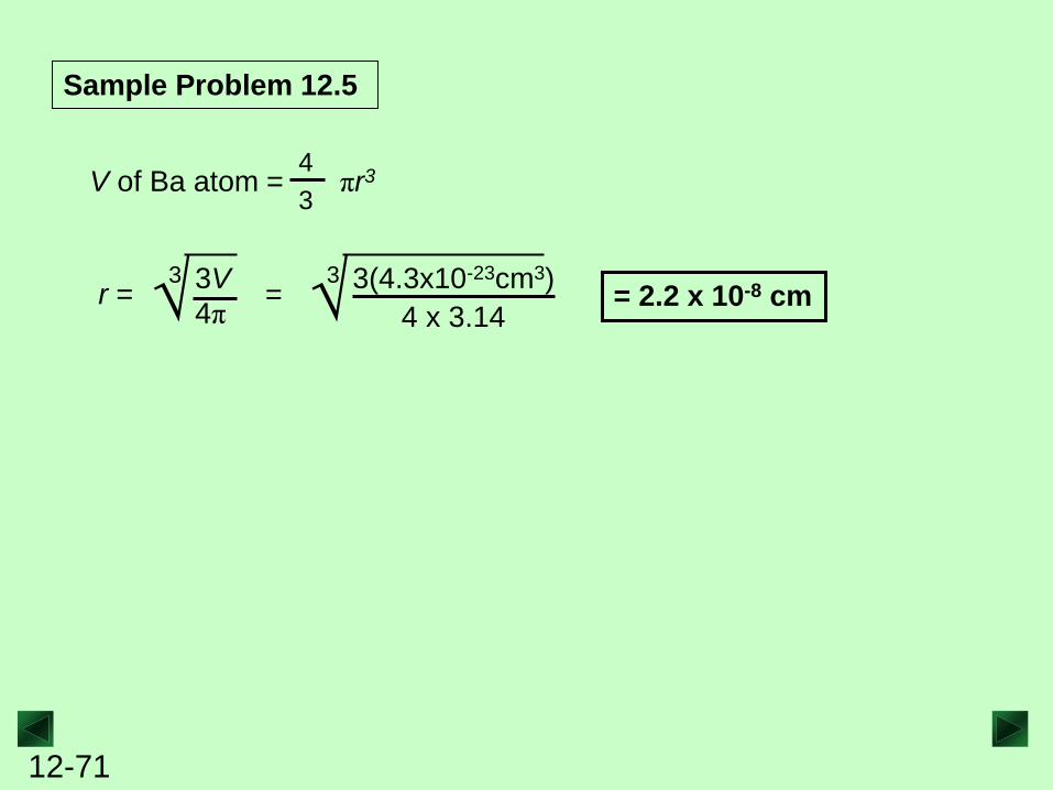
Sample Problem 12.5

V of Ba atom = πr3 4

3

r = 4π √ 3V 3

√ 3 3(4.3x10-23cm3)

4 x 3.14 = = 2.2 x 10-8 cm

12-72

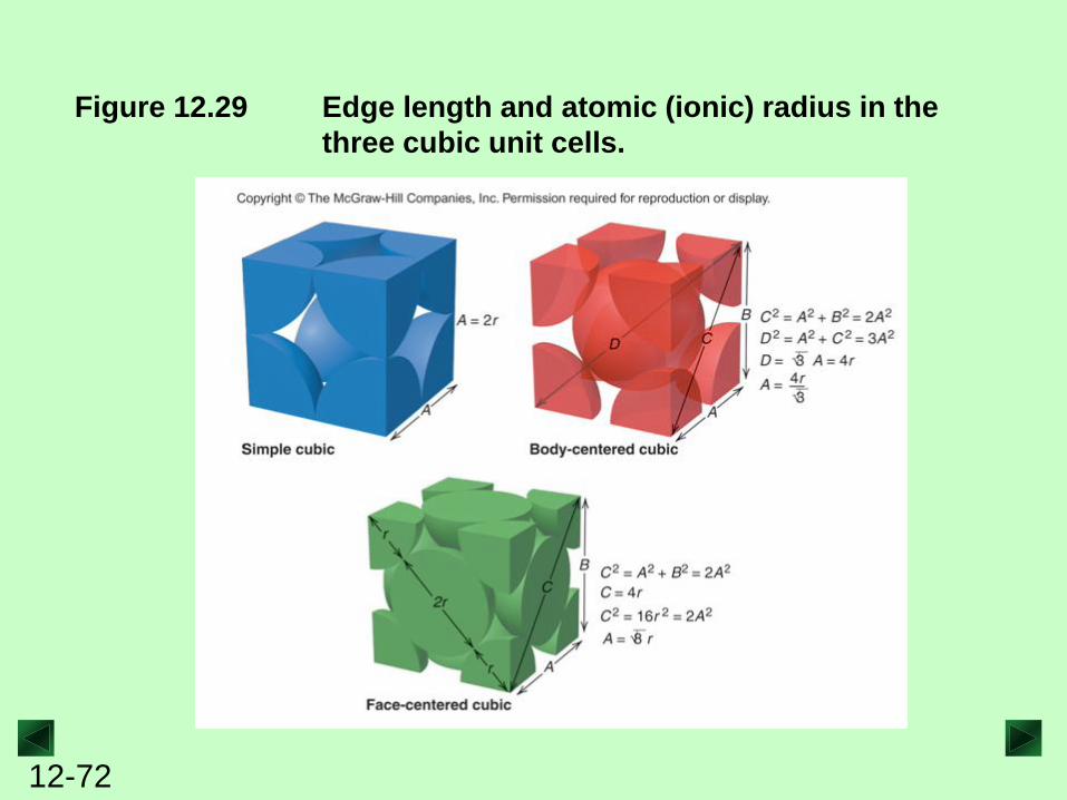
Figure 12.29 Edge length and atomic (ionic) radius in the

three cubic unit cells.

12-73

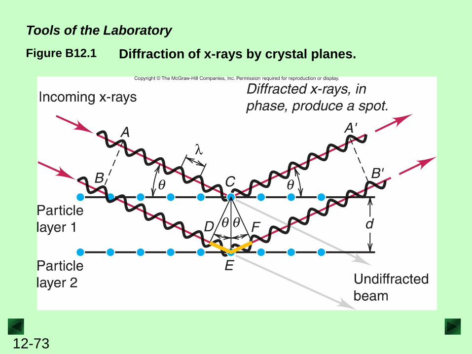
Figure B12.1 Diffraction of x-rays by crystal planes.

Tools of the Laboratory

12-74

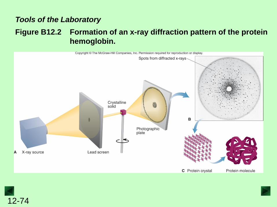
Figure B12.2 Formation of an x-ray diffraction pattern of the protein

hemoglobin.

Tools of the Laboratory

12-75

Tools of the Laboratory

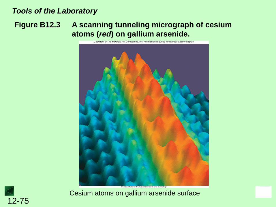
Figure B12.3 A scanning tunneling micrograph of cesium

atoms (red) on gallium arsenide.

Cesium atoms on gallium arsenide surface

12-76

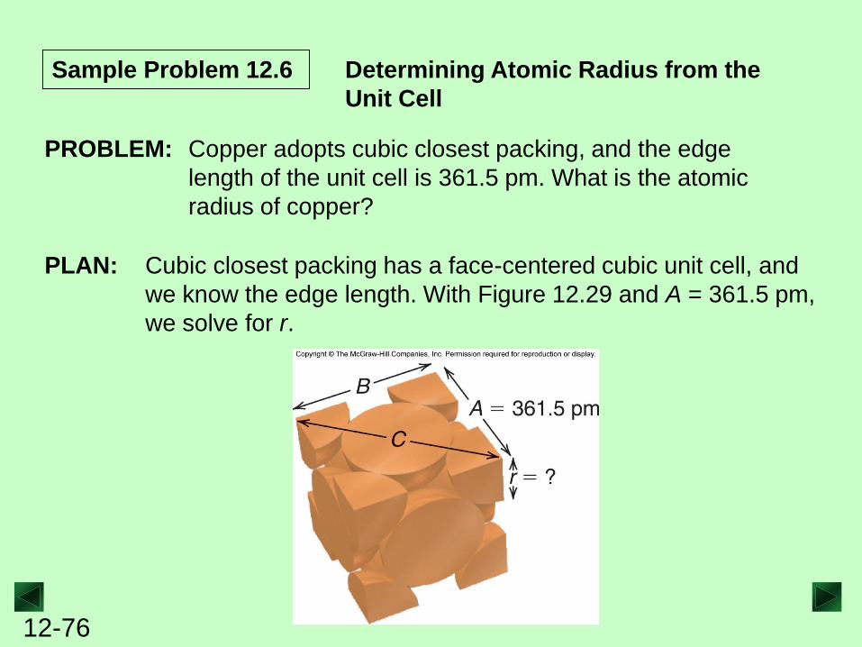
Sample Problem 12.6 Determining Atomic Radius from the

Unit Cell

PLAN: Cubic closest packing has a face-centered cubic unit cell, and

we know the edge length. With Figure 12.29 and A = 361.5 pm,

we solve for r.

PROBLEM: Copper adopts cubic closest packing, and the edge

length of the unit cell is 361.5 pm. What is the atomic

radius of copper?

12-77

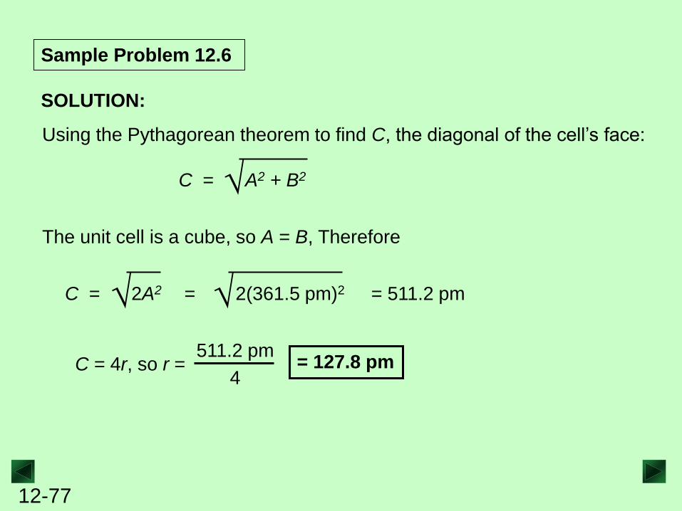
Sample Problem 12.6

SOLUTION:

Using the Pythagorean theorem to find C, the diagonal of the cell’s face:

C = A2 + B2 √

The unit cell is a cube, so A = B, Therefore

C = 2A2 √ = 2(361.5 pm)2 √ = 511.2 pm

C = 4r, so r = 511.2 pm

4 = 127.8 pm

12-78

Types of Crystalline Solids

Atomic solids consist of individual atoms held together only

by dispersion forces.

Ionic solids consist of a regular array of cations and anions.

Molecular solids consist of individual molecules held

together by various combinations of intermolecular forces.

Metallic solids have exhibit an organized crystal structure.

Network Covalent solids consist of atoms covalently

bonded together in a three-dimensional network.

12-79

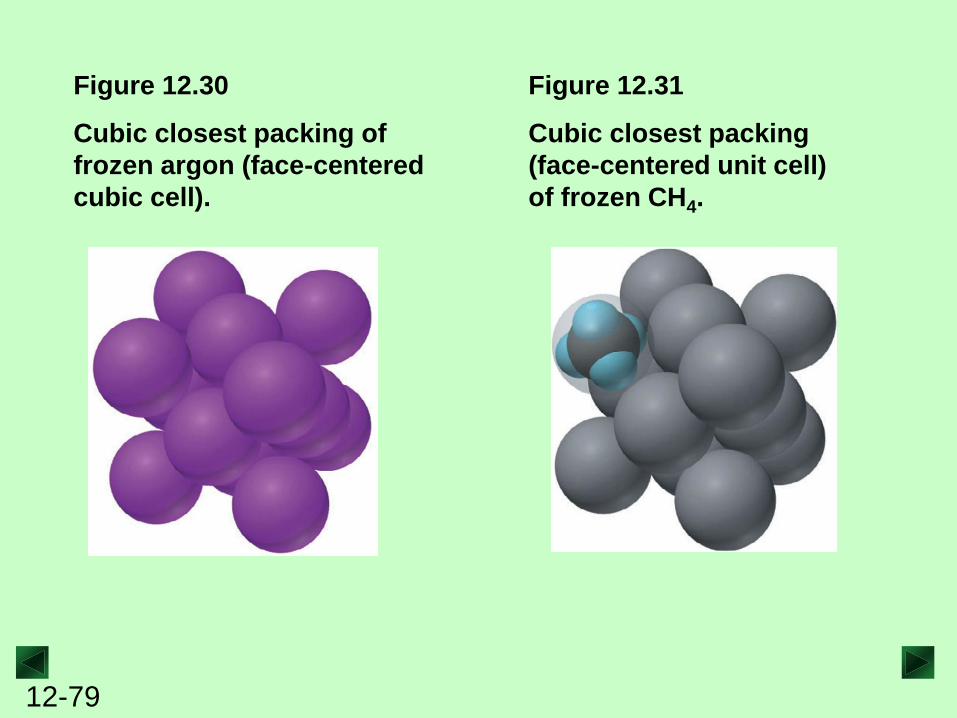
Figure 12.30 Figure 12.31

Cubic closest packing of

frozen argon (face-centered

cubic cell).

Cubic closest packing

(face-centered unit cell)

of frozen CH4.

12-80

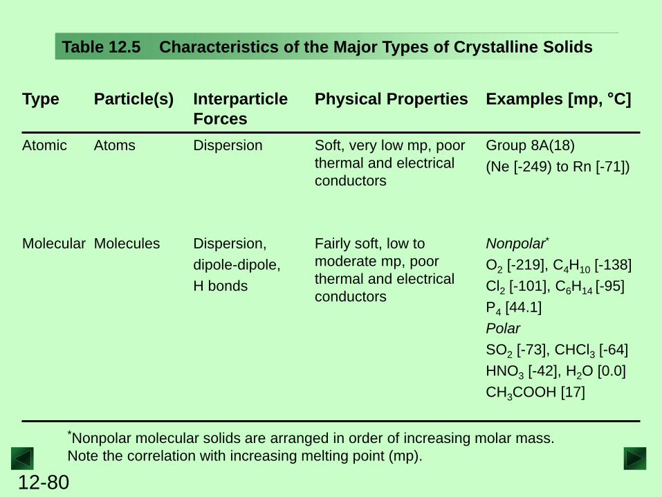
Table 12.5 Characteristics of the Major Types of Crystalline Solids

Type Particle(s) Interparticle

Forces

Physical Properties Examples [mp, °C]

Atomic Atoms Dispersion Soft, very low mp, poor

thermal and electrical

conductors

Group 8A(18)

(Ne [-249) to Rn [-71])

Molecular Molecules Dispersion,

dipole-dipole,

H bonds

Fairly soft, low to

moderate mp, poor

thermal and electrical

conductors

Nonpolar*

O2 [-219], C4H10 [-138]

Cl2 [-101], C6H14 [-95]

P4 [44.1]

Polar

SO2 [-73], CHCl3 [-64]

HNO3 [-42], H2O [0.0]

CH3COOH [17]

*Nonpolar molecular solids are arranged in order of increasing molar mass.

Note the correlation with increasing melting point (mp).

12-81

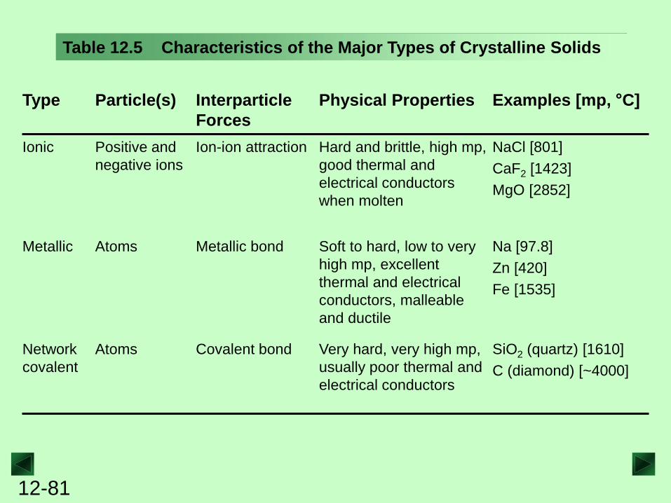
Table 12.5 Characteristics of the Major Types of Crystalline Solids

Type Particle(s) Interparticle

Forces

Physical Properties Examples [mp, °C]

Ionic Positive and

negative ions

Ion-ion attraction Hard and brittle, high mp,

good thermal and

electrical conductors

when molten

NaCl [801]

CaF2 [1423]

MgO [2852]

Metallic Atoms Metallic bond Soft to hard, low to very

high mp, excellent

thermal and electrical

conductors, malleable

and ductile

Na [97.8]

Zn [420]

Fe [1535]

Network

covalent

Atoms Covalent bond Very hard, very high mp,

usually poor thermal and

electrical conductors

SiO2 (quartz) [1610]

C (diamond) [~4000]

12-82

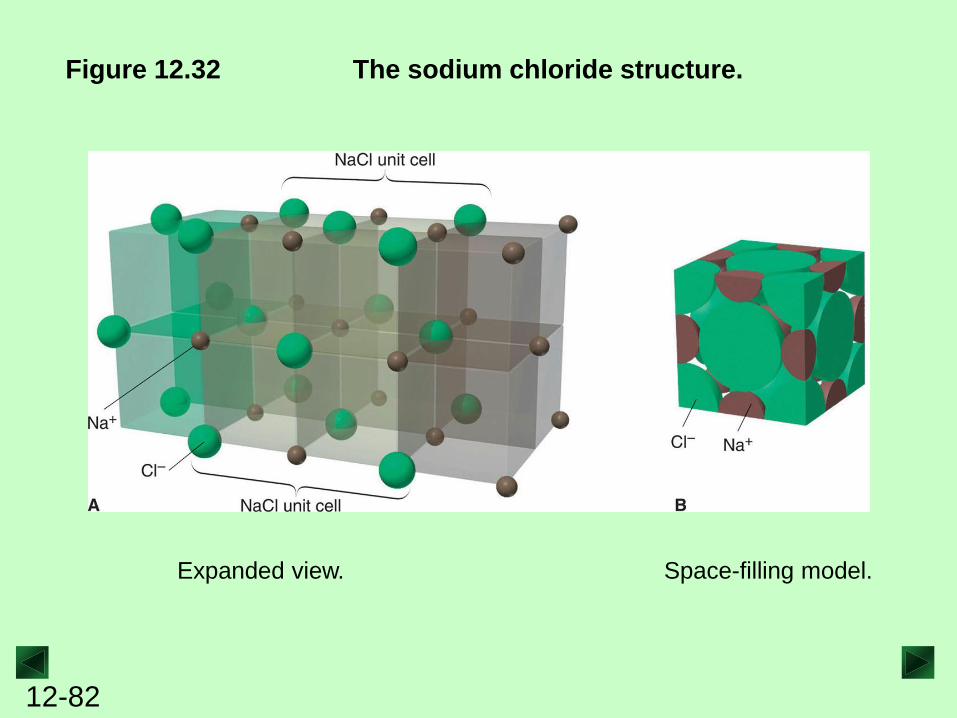
Figure 12.32 The sodium chloride structure.

Expanded view. Space-filling model.

12-83

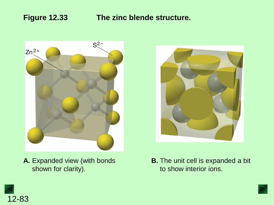
Figure 12.33 The zinc blende structure.

A. Expanded view (with bonds

shown for clarity).

B. The unit cell is expanded a bit

to show interior ions.

12-84

Figure 12.34 The fluorite structure.

A. Expanded view (with bonds

shown for clarity).

B. The unit cell is expanded a bit

to show interior ions.

12-85

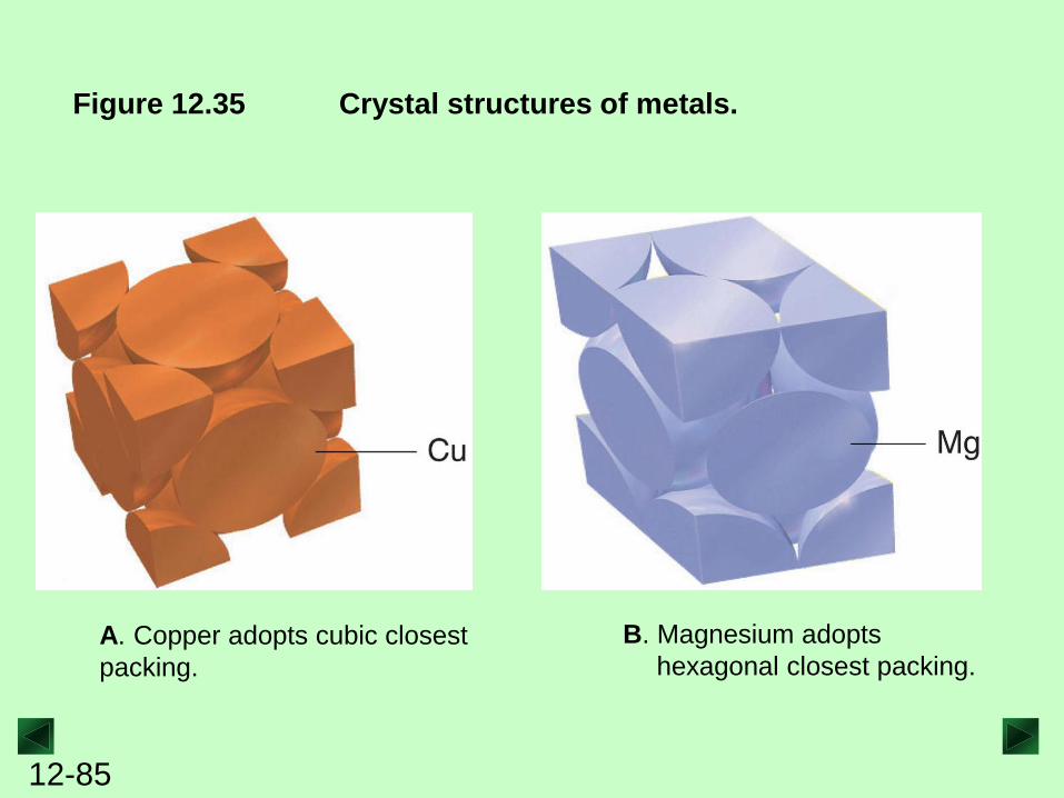
Figure 12.35 Crystal structures of metals.

A. Copper adopts cubic closest

packing.

B. Magnesium adopts

hexagonal closest packing.

12-86

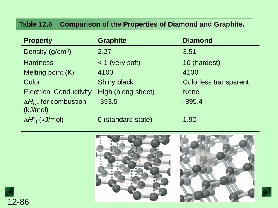
Table 12.6 Comparison of the Properties of Diamond and Graphite.

Property Graphite Diamond

Density (g/cm3) 2.27 3.51

Hardness < 1 (very soft) 10 (hardest)

Melting point (K) 4100 4100

Color Shiny black Colorless transparent

Electrical Conductivity High (along sheet) None

DHrxn for combustion

(kJ/mol)

-393.5 -395.4

DH°f (kJ/mol)

0 (standard state) 1.90

12-87

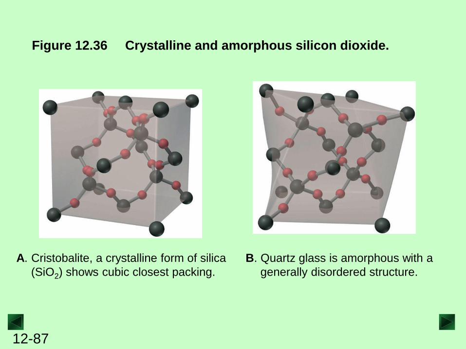
Figure 12.36 Crystalline and amorphous silicon dioxide.

A. Cristobalite, a crystalline form of silica

(SiO2) shows cubic closest packing.

B. Quartz glass is amorphous with a

generally disordered structure.

12-88

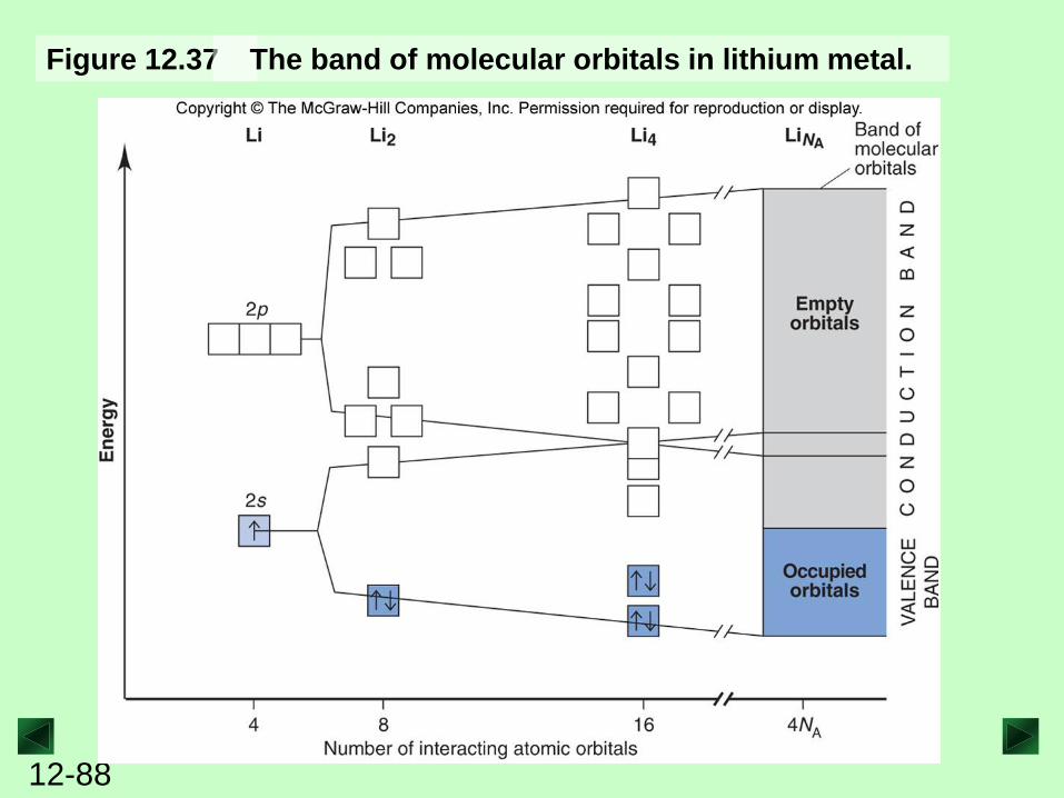
Figure 12.37 The band of molecular orbitals in lithium metal.

12-89

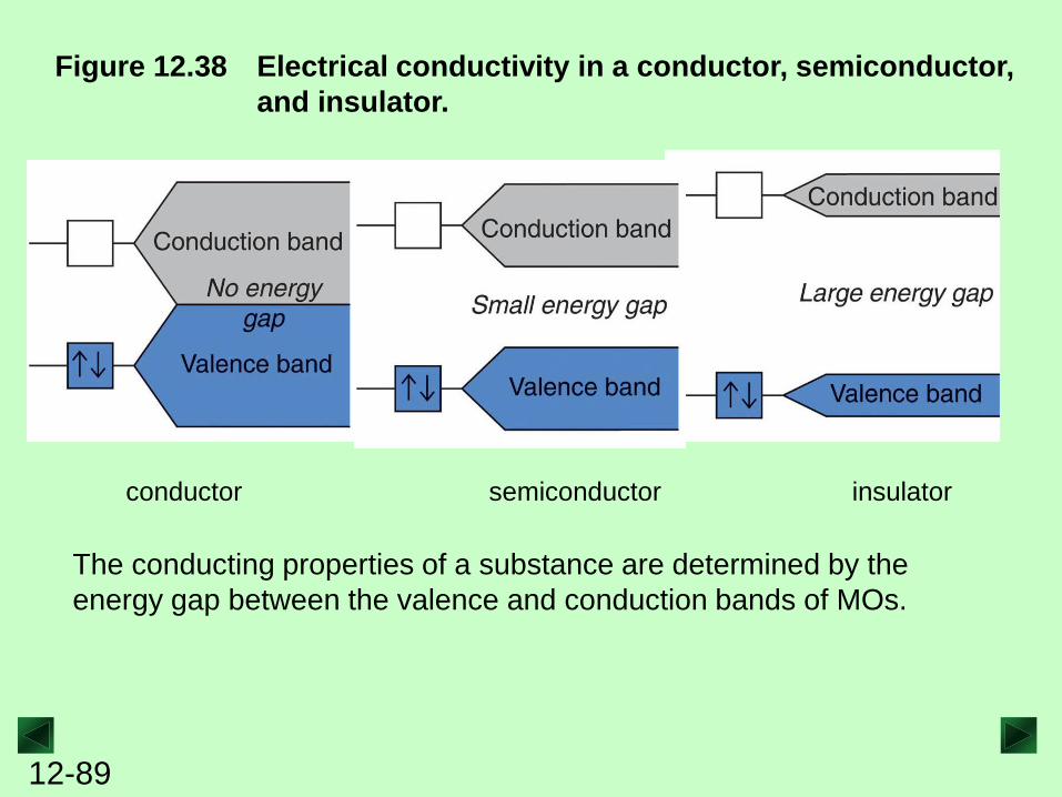
Figure 12.38 Electrical conductivity in a conductor, semiconductor,

and insulator.

conductor semiconductor insulator

The conducting properties of a substance are determined by the

energy gap between the valence and conduction bands of MOs.

12-90

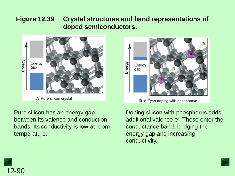
Figure 12.39 Crystal structures and band representations of

doped semiconductors.

Pure silicon has an energy gap

between its valence and conduction

bands. Its conductivity is low at room

temperature.

Doping silicon with phosphorus adds

additional valence e-. These enter the

conductance band, bridging the

energy gap and increasing

conductivity.

12-91

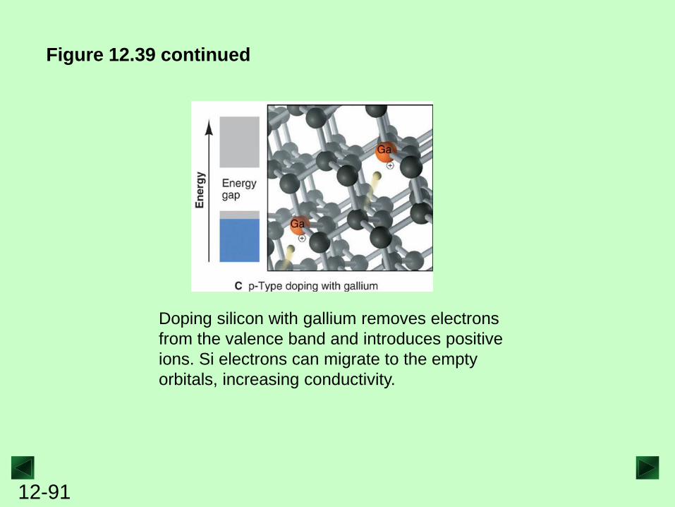
Figure 12.39 continued

Doping silicon with gallium removes electrons

from the valence band and introduces positive

ions. Si electrons can migrate to the empty

orbitals, increasing conductivity.

12-92

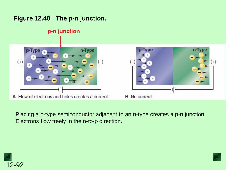
p-n junction

Figure 12.40 The p-n junction.

Placing a p-type semiconductor adjacent to an n-type creates a p-n junction.

Electrons flow freely in the n-to-p direction.

12-93

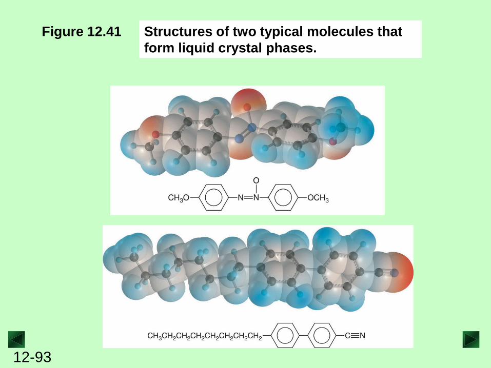
Figure 12.41 Structures of two typical molecules that

form liquid crystal phases.

12-94

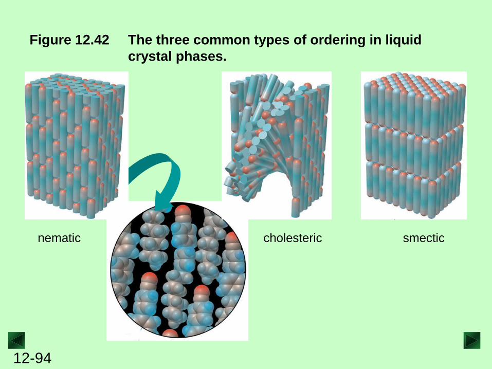
Figure 12.42 The three common types of ordering in liquid

crystal phases.

nematic smectic cholesteric

12-95

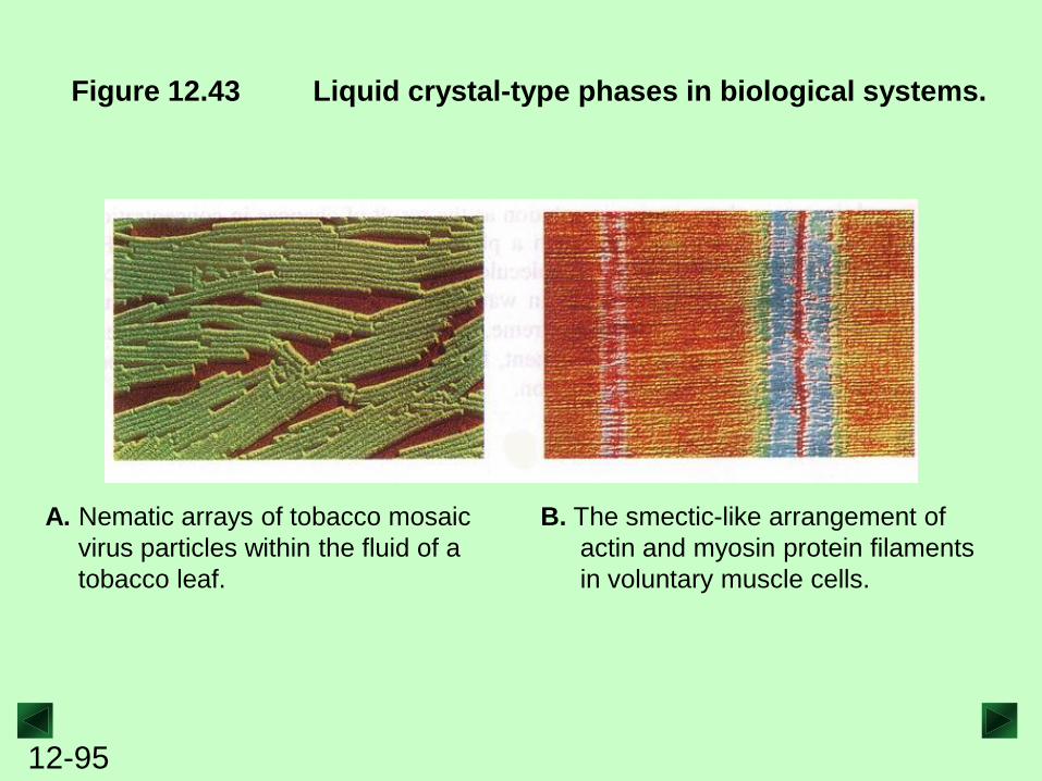
Figure 12.43 Liquid crystal-type phases in biological systems.

A. Nematic arrays of tobacco mosaic

virus particles within the fluid of a

tobacco leaf.

B. The smectic-like arrangement of

actin and myosin protein filaments

in voluntary muscle cells.

12-96

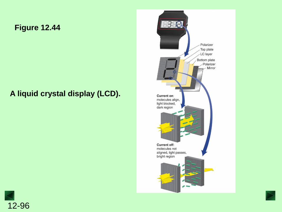
Figure 12.44

A liquid crystal display (LCD).

12-97

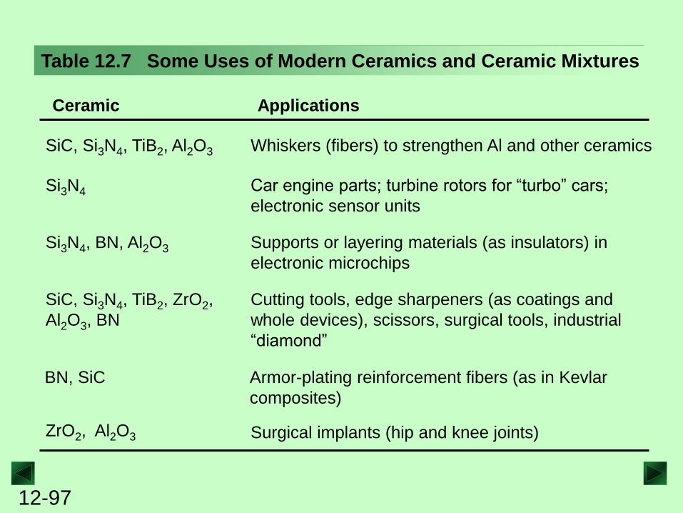
Table 12.7 Some Uses of Modern Ceramics and Ceramic Mixtures

Ceramic Applications

SiC, Si3N4, TiB2, Al2O3 Whiskers (fibers) to strengthen Al and other ceramics

Si3N4 Car engine parts; turbine rotors for “turbo” cars;

electronic sensor units

Si3N4, BN, Al2O3 Supports or layering materials (as insulators) in

electronic microchips

SiC, Si3N4, TiB2, ZrO2,

Al2O3, BN

ZrO2, Al2O3

Cutting tools, edge sharpeners (as coatings and

whole devices), scissors, surgical tools, industrial

“diamond”

BN, SiC Armor-plating reinforcement fibers (as in Kevlar

composites)

Surgical implants (hip and knee joints)

12-98

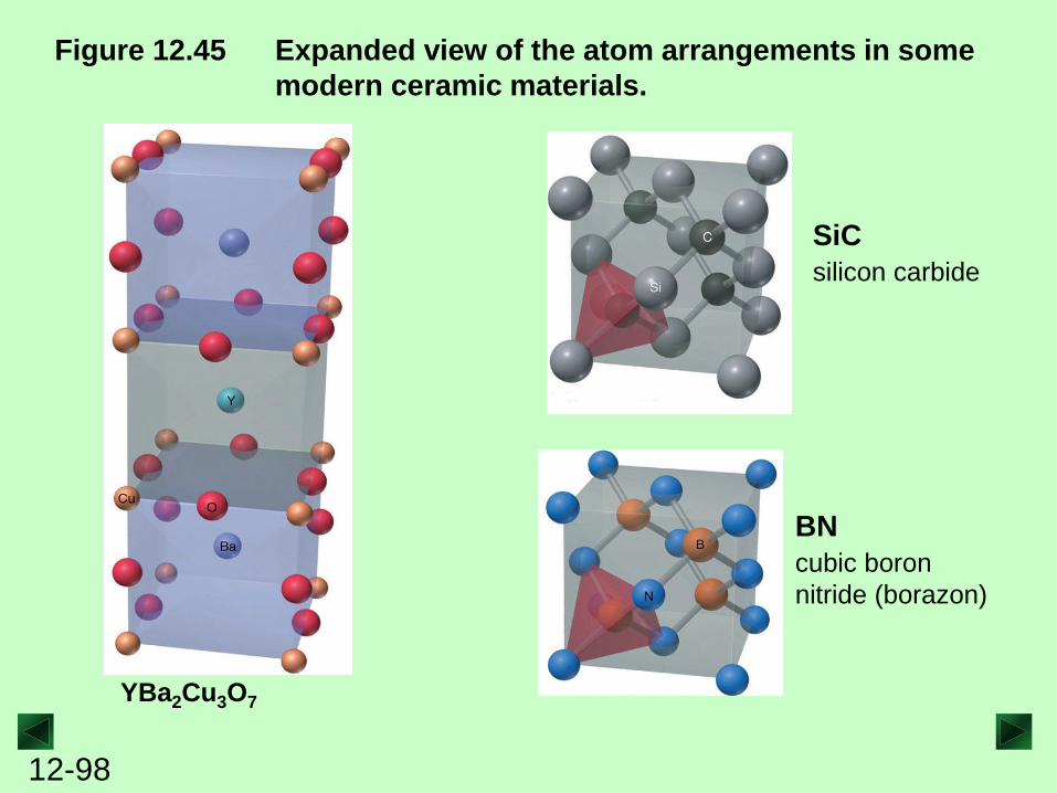
Figure 12.45 Expanded view of the atom arrangements in some

modern ceramic materials.

SiC

silicon carbide

BN

cubic boron

nitride (borazon)

YBa2Cu3O7

12-99

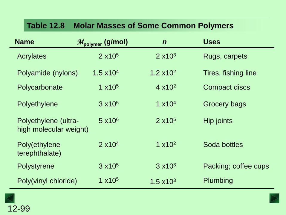
Table 12.8 Molar Masses of Some Common Polymers

Name Mpolymer (g/mol) n Uses

Acrylates 2 x105 2 x103 Rugs, carpets

Polyamide (nylons) 1.5 x104 1.2 x102 Tires, fishing line

Polycarbonate 1 x105 4 x102 Compact discs

Polyethylene 3 x105 1 x104 Grocery bags

Polyethylene (ultra-

high molecular weight)

5 x106 2 x105 Hip joints

Poly(ethylene

terephthalate)

2 x104 1 x102 Soda bottles

Polystyrene 3 x105 3 x103 Packing; coffee cups

Poly(vinyl chloride) 1 x105 1.5 x103 Plumbing

12-

100

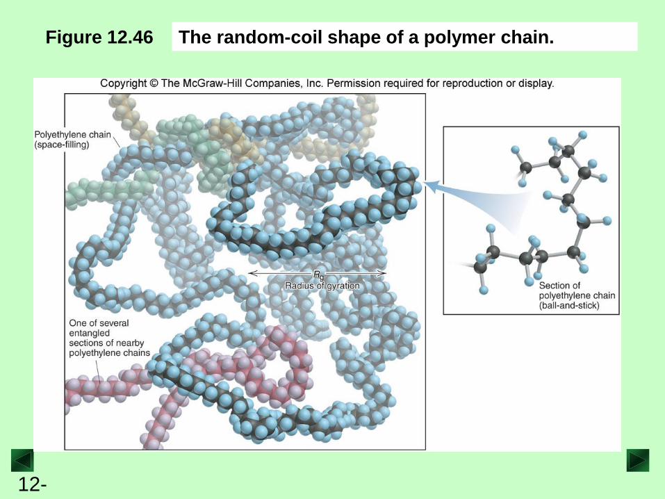
Figure 12.46 The random-coil shape of a polymer chain.

12-

101

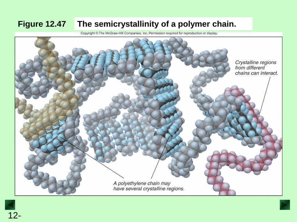
Figure 12.47 The semicrystallinity of a polymer chain.

12-

102

Figure 12.48 The viscosity of a polymer in aqueous solution.

12-

103

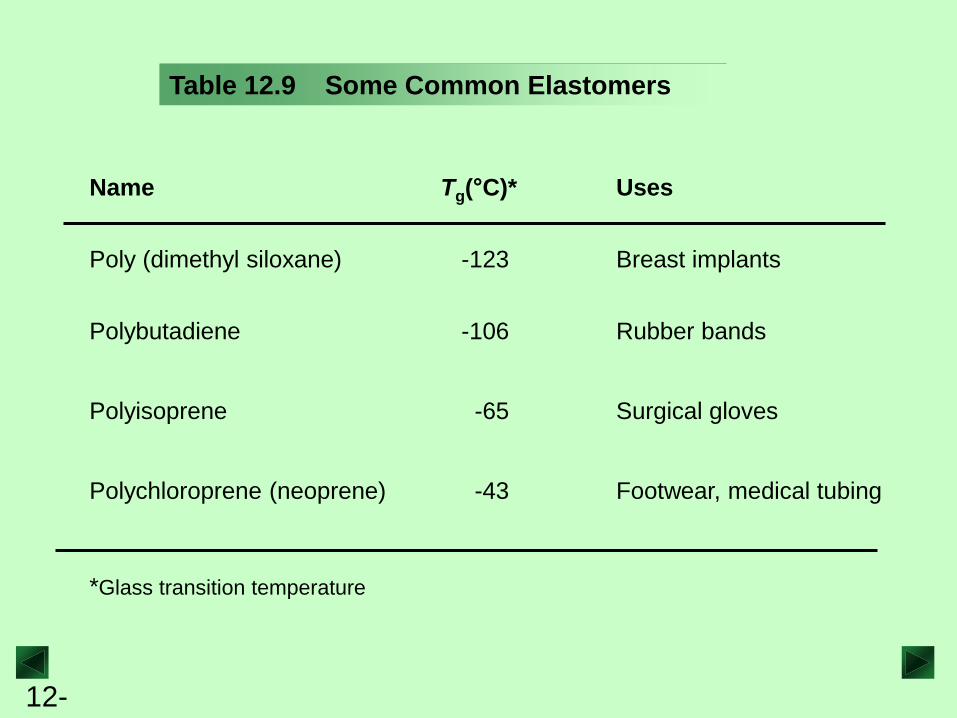
Table 12.9 Some Common Elastomers

Name Tg(°C)*

*Glass transition temperature

Uses

Poly (dimethyl siloxane) -123

-106

-65

-43

Polybutadiene

Polyisoprene

Polychloroprene (neoprene)

Breast implants

Rubber bands

Surgical gloves

Footwear, medical tubing

12-

104

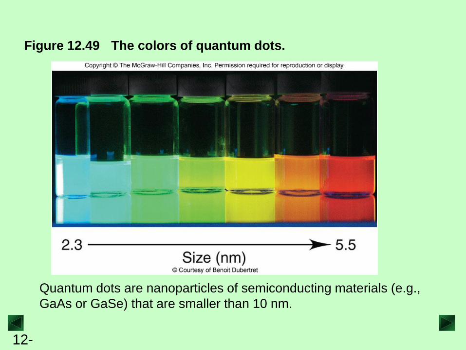
Figure 12.49 The colors of quantum dots.

Quantum dots are nanoparticles of semiconducting materials (e.g.,

GaAs or GaSe) that are smaller than 10 nm.

12-

105

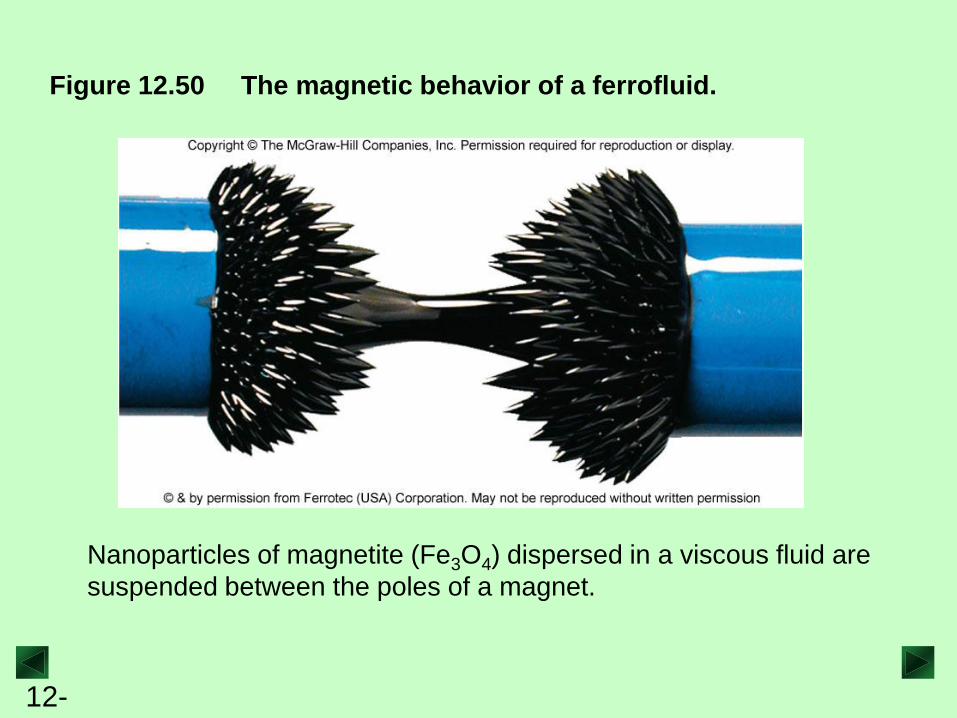
Figure 12.50 The magnetic behavior of a ferrofluid.

Nanoparticles of magnetite (Fe3O4) dispersed in a viscous fluid are

suspended between the poles of a magnet.

12-

106

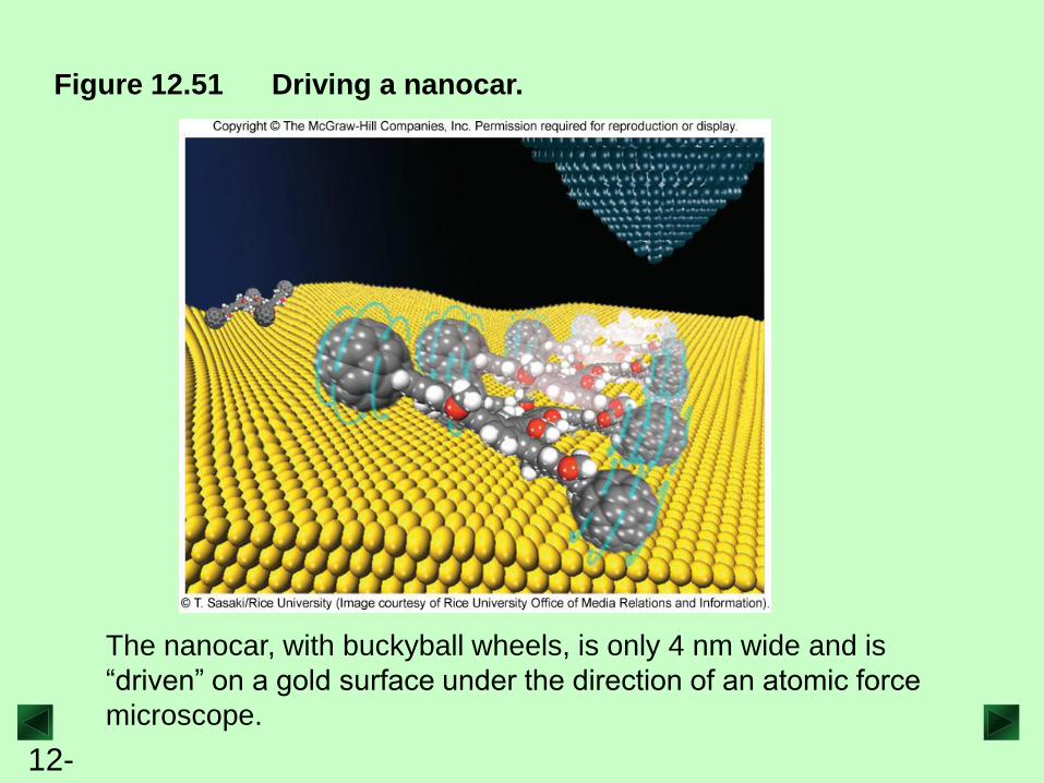
Figure 12.51 Driving a nanocar.

The nanocar, with buckyball wheels, is only 4 nm wide and is

“driven” on a gold surface under the direction of an atomic force

microscope.